


Abstract
The structural safety of polar ships is critically dependent on local ice loads acting in the ship–ice interaction area. Ice conditions and ship speeds play dominant roles in influencing local ice loads. Field measurement serves as a crucial approach for accurately assessing and scientifically understanding local ice loads and ice conditions. The instrumentation for the field measurement on RV Xuelong-2 is discussed in this study. In the 12th Chinese National Arctic Research Expedition, digital processing technologies are employed for image recognition and statistical analysis of ice concentrations and thicknesses. The influence coefficient matrix method is validated by a physical experiment and applied to identify local ice loads from ice-induced strains. Subsequently, the relationship between local ice loads, ice conditions, and ship speeds is statistically analyzed and mechanistically explained. The results show that the coupling effect between ship speeds and ice parameters, along with the competition between ice failure modes, may cause ice load peaks to transition from increasing to decreasing at a specific ship speed and ice thickness. A prolonged ice load duration under high ice concentrations is an important factor contributing to the positive correlation between ice load peaks and ice concentrations.
1. Introduction
In recent years, global warming has accelerated the melting of Arctic sea ice [1]. Against the backdrop of continuously deepening economic globalization and regional integration, the Arctic has been gaining increasing strategic, economic, scientific, environmental, navigational, and resource-related value, attracting widespread attention from the international community [2]. Polar ships are essential equipment for understanding, protecting, and utilizing the Arctic. During navigation through ice-covered waters, polar ships are subjected primarily to ice loads [3]. Unlike global ice loads that mainly influence resistance, local ice loads in the ship–ice interaction area pose a direct threat to structural integrity, potentially causing severe damage or fatigue failure [4]. To establish Arctic navigation warning systems and design ice-resistant ship structures, it is essential to accurately assess and scientifically understand local ice loads.
Field measurement is regarded as an effective and direct approach to obtain local ice loads, which involves measuring ice-induced structural responses and identifying ice loads through inverse methods [5,6,7]. During navigation in ice regions, the bow, bow shoulder, and stern shoulder of a ship frequently come into contact with sea ice. The side frames in these areas serve as the main load-bearing components, and the internal normal and shear strains are key parameters for measuring ice-induced structural responses [8]. In terms of inverse methods, John and Daley [9] initially utilized beam theory to establish a proportional relationship between the shear strain and ice load on a frame, identifying the ice load by the difference in shear strains at both ends of the frame. Kujala and Vuorio [10] further considered scenarios where ice loads act simultaneously on multiple frames, taking into account the influence of ice loads acting on adjacent frames on the structural response of each frame. Assuming a uniform distribution of ice loads across each subarea in the instrumented region, the influence coefficient matrix method was formulated on the basis of mechanical analysis. Owing to its concise formulation, efficient computation, and accurate results, this method has been predominantly used for the real-time identification of local ice loads [11,12,13].
Ship speeds and ice conditions serve as the primary factors that affect local ice loads. Therefore, it is necessary to conduct synchronous monitoring of both during Arctic navigation [14]. The former can be easily recorded by GPS, while the latter is difficult to be obtained through manual observation due to the extreme geographical location and harsh climatic conditions of the Arctic. As a result, satellite remote sensing [15,16,17], radar remote sensing [18,19,20], and shipborne photographic observation [21,22] become widely adopted alternatives. Among these, shipborne photographic observation is particularly suitable for concurrent implementation in field measurements of local ice loads due to its intuitive and real-time characteristics. Through digital processing technologies, ice parameters such as thickness and concentration can be extracted from sea ice images, avoiding the recognition errors associated with manual visual inspection [23]. In recent years, the rapid development of machine learning algorithms in ocean engineering [24], such as support vector machine [25,26] and deep neural network [27,28], has provided new approaches for image recognition, contributing to real-time acquisition of ice parameters during Arctic navigation.
In the study of the relationship between local ice loads, ship speeds, and ice conditions, Uto et al. [29] discussed the correlation of ice load peaks with ship speeds based on the measured data from PM Teshio. During continuous icebreaking, the ice load peaks at the bow are highly dependent on ship speeds. The higher the speed, the greater the added mass of ice floes, resulting in an increase in bow ice loads. The research on Louis S. St. Laurent indicated that ice loads are positively correlated with ice concentrations at a constant speed. In the same range of ice concentrations, greater ice thicknesses generally lead to lower speeds and result in smaller ice loads [30]. According to Hänninen et al. [31], a weak linear relationship exists between ice load peaks and ship speeds; however, the mean values of ice loads decline as ship speeds increase, regardless of ice thicknesses. However, there are also cases that contradict the above views. Frederking [32] found that only high speeds exceeding 10 m/s would lead to an increase in ice loads. Unusually high load peaks also existed at ice thicknesses as low as 0.2 m [33]. Because ship–ice interactions are inherently random and measured data exhibit significant scatter, no definitive conclusion has been reached regarding how local ice loads relate to ship speeds and ice conditions.
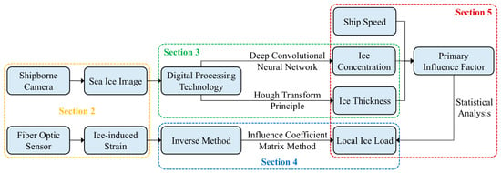
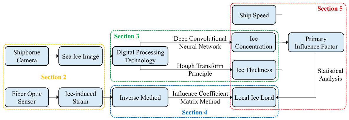
Since the late 1970s, countries around the Arctic have carried out extensive field measurements on their polar ships [34,35,36]. In 2014, China began to measure local ice loads and ice conditions on RV Xuelong during its polar research expedition [5,6]. Further, a real-time monitoring system was equipped on RV Xuelong-2 in 2019 [37]. The system integrates multiple data sources such as meteorology, hydrology, GPS, compass, ice conditions, and structural responses. The present study focuses on discussing the measurement methods of ice conditions and ice-induced strains in the system. Based on the measured data from the 12th Chinese National Arctic Research Expedition (CHINARE-Arctic), digital processing technologies are applied to perform image recognition and statistical analysis of ice concentrations and thicknesses. The influence coefficient matrix method is validated by a physical experiment and applied to identify local ice loads from ice-induced strains. Finally, the relationship between local ice loads, ship speeds, and ice conditions is statistically analyzed and mechanistically explained. The technical route of the research is shown in Figure 1.
Figure 1.
Technical route of the research.
2. Instrumentation for the Field Measurement on RV Xuelong-2
RV Xuelong-2 is China’s first domestically built polar research vessel. With the ice class of PC3, it is capable of continuously navigating either ahead or astern at a speed of 2–3 kn in the environment with an ice thickness of 1.5 m and a snow thickness of 0.2 m. On 12 July 2021, the ship departed from Shanghai to begin the 12th CHINARE-Arctic. The voyage in ice-covered waters lasted 35 days, from 28 July to 2 September.
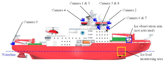
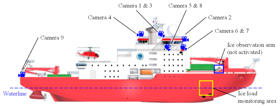
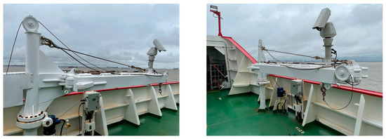
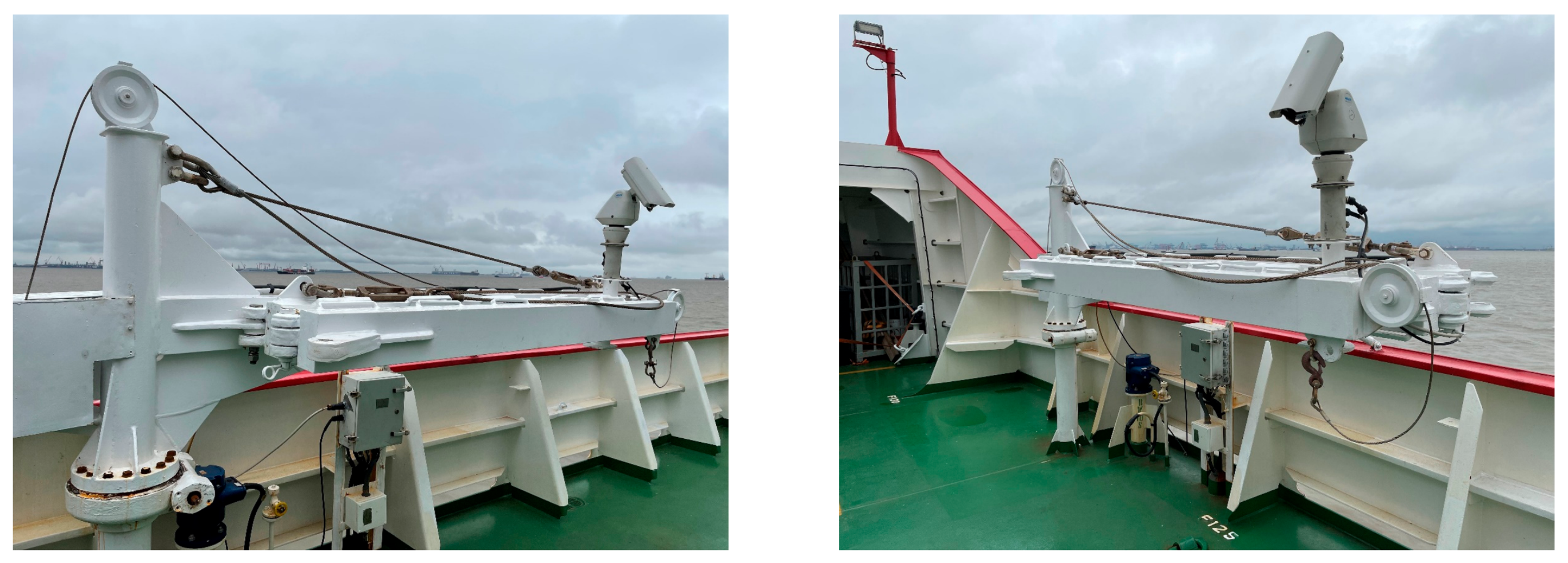
Nine cameras were mounted around the bridge and compass deck to capture ice conditions from multiple perspectives along the route, enabling the acquisition of ice parameters including concentration, thickness, type, and floe size. The distribution of these shipborne cameras is depicted in Figure 2. The location of each camera and its identified ice parameters are listed in Table 1. Images were collected from all cameras at 10 s intervals, and videos were captured by Cameras 2, 5, and 8 in 60 s lengths. Additionally, an ice observation arm located on the starboard deck (see Figure 3) could be extended outside the hull to observe ship–ice interaction processes at close range, but it was not activated during this voyage.
Figure 2.
Distribution of shipborne cameras and ice load monitoring area on RV Xuelong-2.
Table 1.
Locations of shipborne cameras and their identified ice parameters.
Figure 3.
Ice observation arm located on the starboard deck of RV Xuelong-2 (not activated).
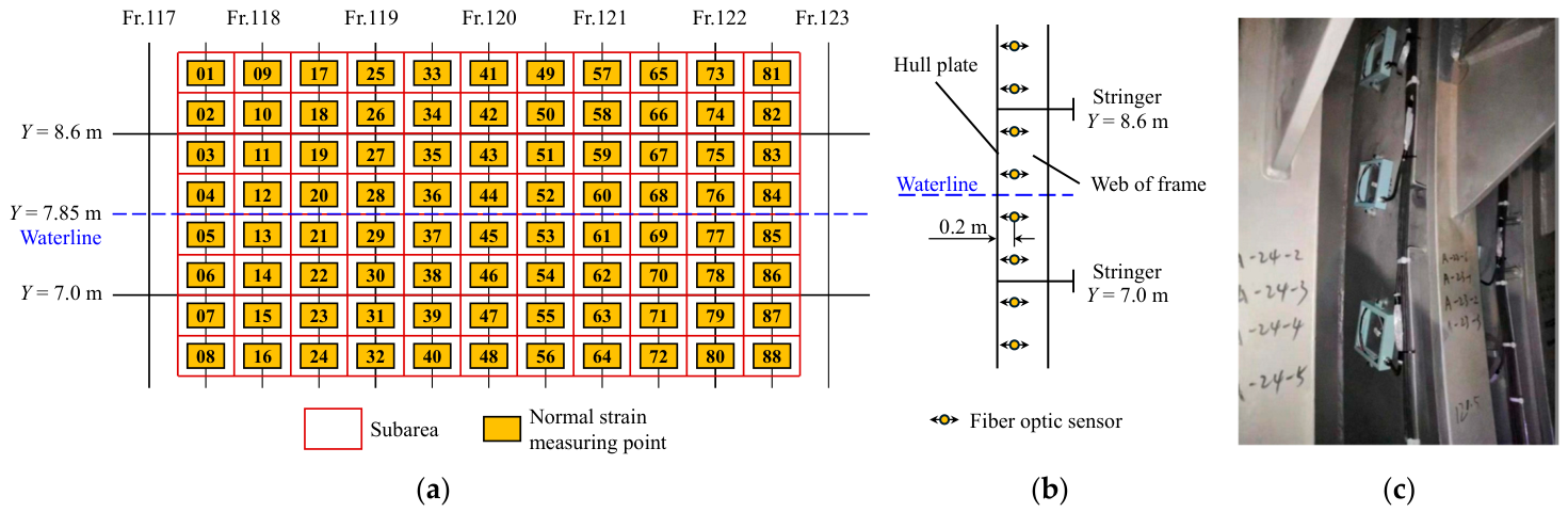
The bow shoulder—an area of frequent ship–ice interactions—was chosen for the ice load monitoring on RV Xuelong-2, covering a total area of 14 m2 (see Figure 2). This area lies on the hull plate of the No. 10 ballast tank, close to the waterline. Fiber optic sensors installed on the frames in this area were used to measure ice-induced strains.
In earlier measurements, shear strains were typically measured using a right-angle rosette placed near each end of a frame, and the ice load on that frame was then identified from the shear strain difference. However, the exact location of the ice load on the frame cannot be determined. During the field measurement on Timofey Guzhenko, an alternative method based on normal strain measurements was developed to address this limitation [38,39]. Compared with shear strains, normal strain measuring points can be deployed more flexibly at multiple locations on a frame, enhancing the refinement of ice load monitoring.
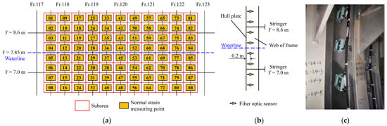
Consequently, the ice load monitoring area of RV Xuelong-2 was partitioned into 88 subareas, and 88 normal strain measuring points were correspondingly arranged densely on the webs of 11 frames (see Figure 4a). Based on the sensitivity study on the deployment of measuring points [8] and considering the construction difficulties in tight spaces, fiber optic sensors were placed vertically near the hull plate (0.2 m) to measure normal strains (see Figure 4b).
Figure 4.
Instrumentation for the field measurement of local ice loads on RV Xuelong-2. (a) Distribution of normal strain measuring points in the ice load monitoring area; (b) location of fiber optic sensors on the web of a frame; (c) fiber optic sensors after installation.
3. Recognition and Analysis of Ice Parameters Based on Shipborne Photographic Observation
The ice conditions around a ship are directly related to the magnitude of local ice loads. Effective observation of ice conditions and accurate recognition of ice parameters serve as necessary prerequisites for investigating the relationship between local ice loads and ice conditions. As the most intuitive ice parameters for navigation safety, ice concentrations and thicknesses are extracted from sea ice images through digital processing technologies, and their distribution characteristics during this voyage are analyzed.
3.1. Image Recognition and Statistical Analysis of Ice Concentrations
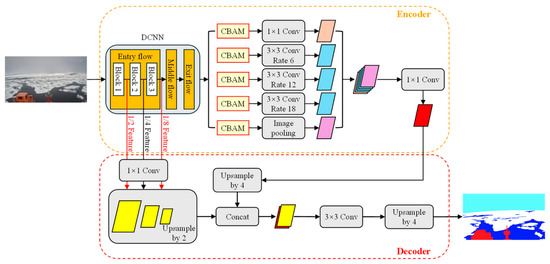
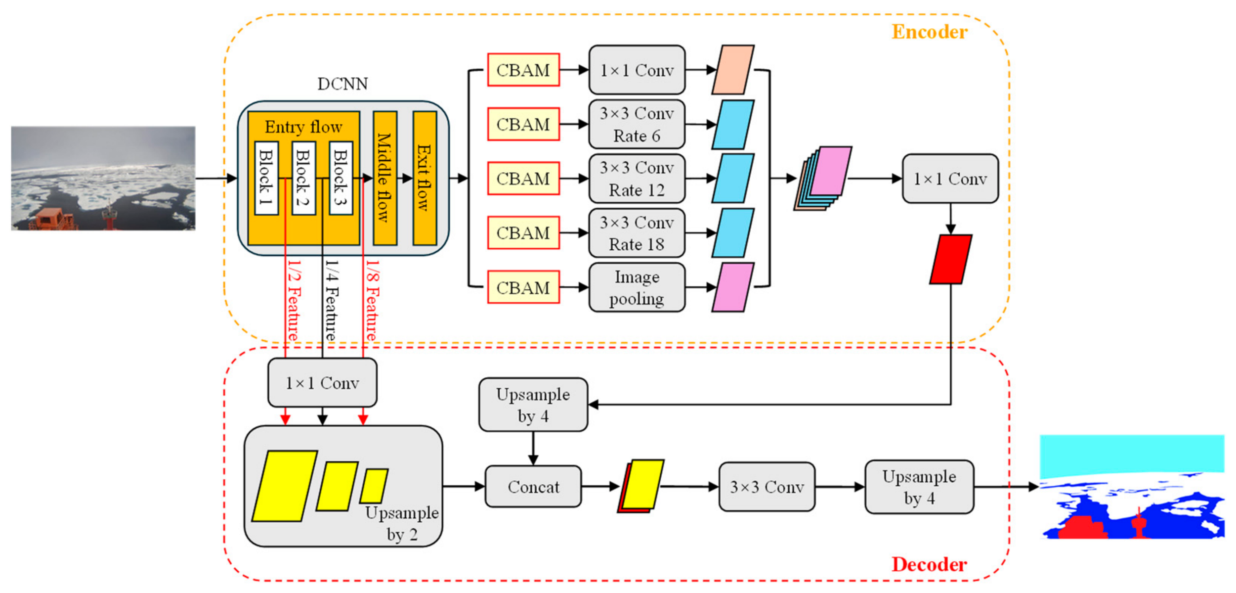
A deep convolutional neural network (DCNN) named Ice-Deeplab is adopted for semantic segmentation of sea ice images [26], which can accurately distinguish the ship, sea ice, seawater, and sky in the images. The network adopts Deeplab V3+ as its basic architecture. To explicitly capture representative feature maps and refine segmentation results, a convolution block attention module (CBAM) is incorporated into the atrous spatial pyramid pooling module, and extra shallow layer features are added to the decoder branch. The overall architecture of Ice-Deeplab is illustrated in Figure 5.
Figure 5.
Overall architecture of Ice-Deeplab for semantic segmentation of sea ice images.
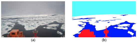
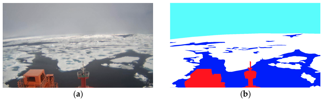
The runtime environment is established based on TensorFlow using CUDA 10.0 and Python 3.6. The hyperparameter settings for network training are listed in Table 2. The dataset consists of 186 sea ice images annotated using LabelMe, with 80% for training and 20% for testing. Mean pixel accuracy (MPA), intersection over union (IoU), and mean intersection over union (MIoU) are used to evaluate the segmentation performance of the network. As shown in Figure 6 and Table 3, the network achieves an IoU of 94.2% for sea ice, with MIoU and MPA both exceeding 90%, which indicates high segmentation accuracy.
Table 2.
Hyperparameter settings for network training of Ice-Deeplab.
Figure 6.
Semantic segmentation of sea ice images by Ice-Deeplab. (a) Original image; (b) segmented image.
Table 3.
Segmentation results of Ice-Deeplab.
Since the shooting angle of the camera is not perpendicular to the ice surface, it is necessary to determine the correspondence between the image plane and sea level according to camera parameters such as height, focal length, pitch angle, and view angle. On this basis, projection correction is performed on the segmented images to eliminate the recognition errors caused by perspective distortion [40]. In addition, the distant ice leads in the image may be shielded by ice floes due to severe perspective distortion, resulting in a large deviation of ice concentrations. To improve the reliability of the recognition results and avoid misleading the risk assessment and route planning, the ice concentration is only calculated in the lower half of the image, which is closer to the camera and features less perspective distortion.
Features of sea ice and seawater are extracted from segmented images after projection correction. The ice concentration is determined by computing the pixel ratio presented in the following equation [26]:
where and are the pixel counts of sea ice and seawater in a segmented image, respectively.
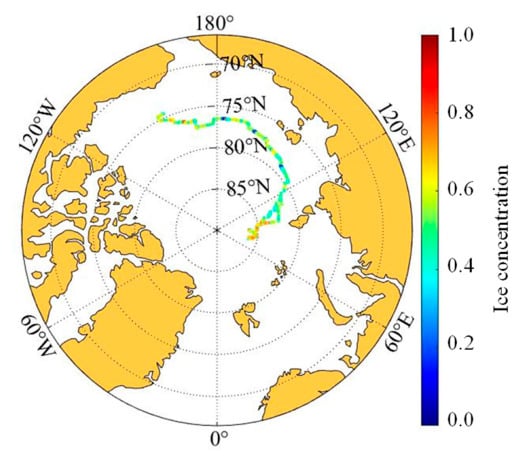
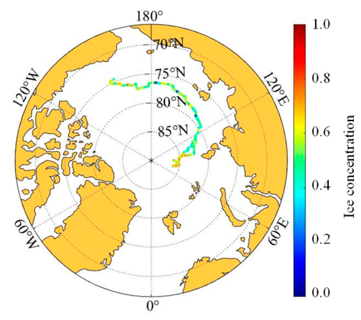
Based on the above principles, systematic recognition is carried out on the sea ice images captured by shipborne cameras throughout the voyage, and the distribution of ice concentrations along the route is obtained, as depicted in Figure 7. The ice concentrations near the North Pole are relatively high, typically exceeding 0.7, while the distribution in other sections of the route is relatively uniform, with no clear increasing trend as the latitude rises.
Figure 7.
Distribution of ice concentrations along the route during the 12th CHINARE-Arctic.
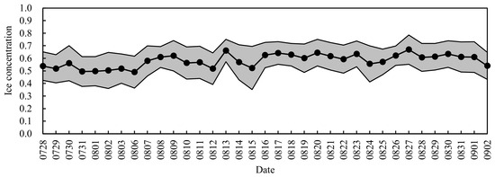
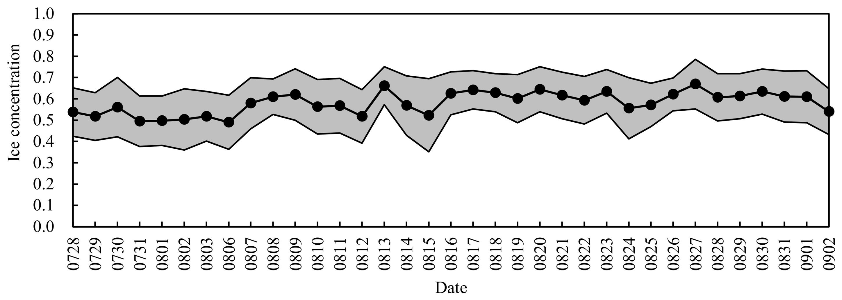
Figure 8 presents the daily fluctuation of the mean values of ice concentrations during the voyage in ice-covered waters. The mean values oscillate around 0.58, with a fluctuation amplitude of 0.13 and a coefficient of variation of 0.22. Compared with ice thicknesses (see Section 3.2), the overall distribution of ice concentrations is relatively concentrated.
Figure 8.
Daily fluctuation of the mean values of ice concentrations during the voyage in ice-covered waters.
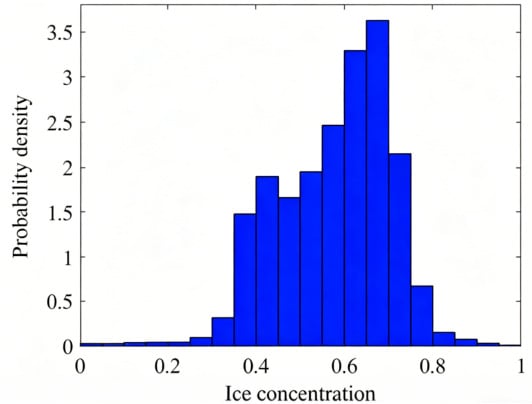
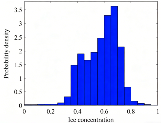
Further analysis is conducted on the probability distribution of 319,886 groups of ice concentration data. As depicted in Figure 9, the ice concentration mainly distributes in the range of 0.4–0.8. Its probability density rises first and then declines, reaching its maximum value in the interval of 0.6–0.7.
Figure 9.
Probability distribution of ice concentrations during the voyage in ice-covered waters.
3.2. Image Recognition and Statistical Analysis of Ice Thicknesses
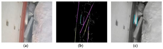
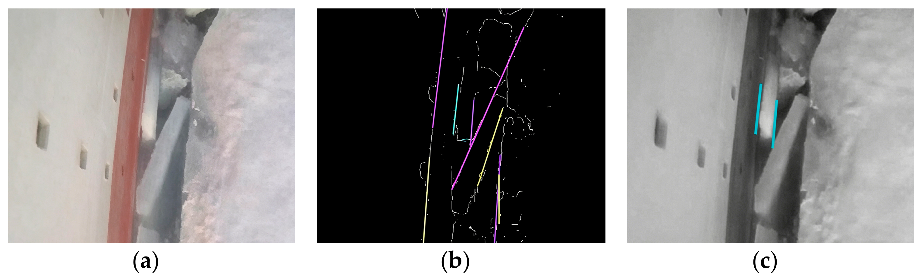
During an icebreaking process, sea ice that breaks off due to bending failure will flip over from the bow and slide to the side of a ship. Therefore, ice thicknesses can be extracted by recognizing the parallel lines at the section edges of flipped ice blocks in sea ice images [41], as shown in Figure 10. First, the section edges of flipped ice blocks are detected using the Sobel operator according to the grayscale gradient variation in the image. Then, straight-line segments in the section edges are extracted through the Hough transform principle. Finally, parallel lines among the straight-line segments are screened according to geometric judgment conditions.
Figure 10.
Recognition of the parallel lines at the section edges of flipped ice blocks by Hough transform principle. (a) Original image; (b) Hough transform; (c) recognition result.
Since the distance between the parallel lines in the image does not represent the actual ice thickness, a scale conversion is performed using a calibration object with a known dimension, as follows:
where is the actual ice thickness, is the actual dimension of the calibration object, and and are the pixel count of the distance between the parallel lines and the dimension of the calibration object in the image, respectively.
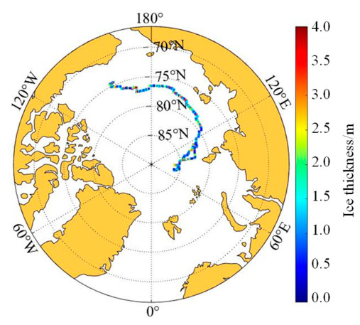
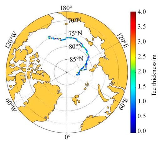
Based on the above principles, systematic recognition is carried out on the sea ice images captured by shipborne cameras throughout the voyage, and the distribution of ice thicknesses along the route is obtained, as depicted in Figure 11. The distribution appears relatively uniform, showing no clear increasing trend with latitude.
Figure 11.
Distribution of ice thicknesses along the route during the 12th CHINARE-Arctic.
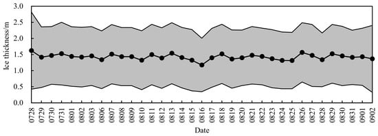
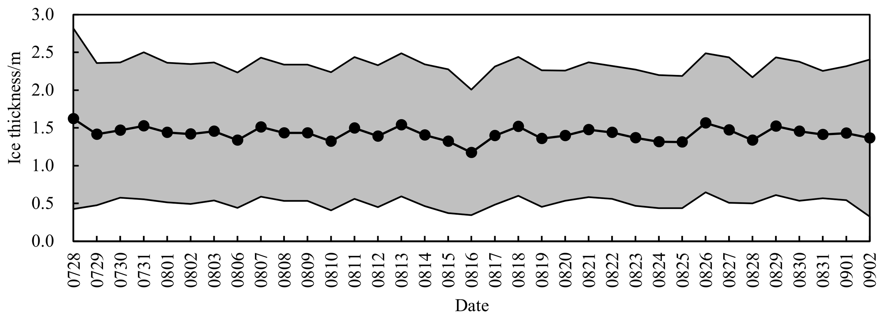
Figure 12 illustrates the daily fluctuation of the mean values of ice thicknesses during the voyage in ice-covered waters. The mean values oscillate around 1.42 m, with a fluctuation amplitude of 0.93 m and a coefficient of variation of 0.65 m. Compared with ice concentrations (see Section 3.1), the overall distribution of ice thicknesses is relatively scattered.
Figure 12.
Daily fluctuation of the mean values of ice thicknesses during the voyage in ice-covered waters.
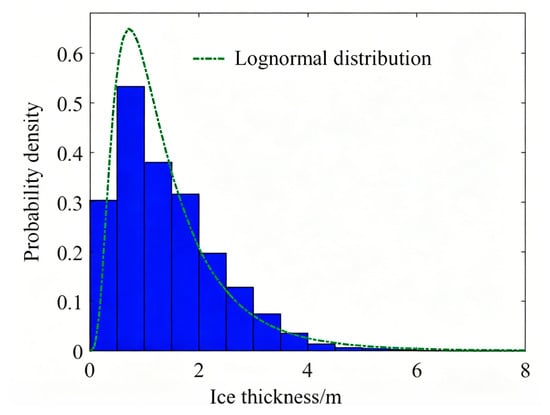
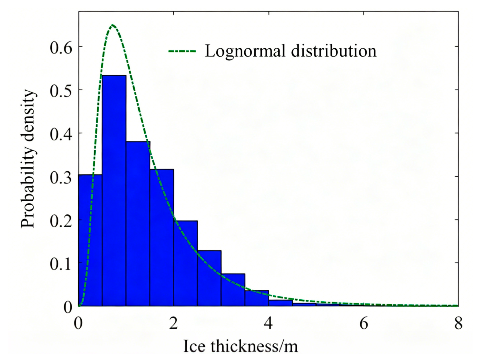
Further analysis is conducted on the probability distribution of 39,017 groups of ice thickness data. As depicted in Figure 13, the ice thickness mainly distributes in the range of 0–3.0 m, which can be approximately characterized by a lognormal distribution. Its probability density rises first and then declines, reaching its maximum value in the interval of 0.5–1.0 m.
Figure 13.
Probability distribution of ice thicknesses during the voyage in ice-covered waters.
4. Identification of Local Ice Loads by Influence Coefficient Matrix Method
4.1. Basic Principle of Influence Coefficient Matrix Method
Based on the linear elastic assumption, it is considered that ice-induced strains are proportional to local ice loads as follows [11,12,13]:
where denotes the ice-induced strain at Measuring Point , represents the ice load acting in the corresponding subarea of Measuring Point , is the influence coefficient matrix, represents the influence of on , , and is the number of measuring points.
The expanded form of Equation (3) is as follows:
If a unit ice load is applied to the corresponding subarea of Measuring Point , and all other subareas remain unloaded, Equation (4) is transformed into the following form:
Here, the -th column of the corresponds to the ice-induced strain at each measuring point under the above loading state. By sequentially applying a unit ice load to every subarea, all elements in the influence coefficient matrix can be obtained.
Thus, local ice loads can be identified by multiplying the influence coefficient matrix by ice-induced strains. Since it is difficult to perform the above loading process on an actual ship, the influence coefficient matrix is usually constructed using a calibrated finite element model of the ship structure.
4.2. Experimental Validation of Influence Coefficient Matrix Method
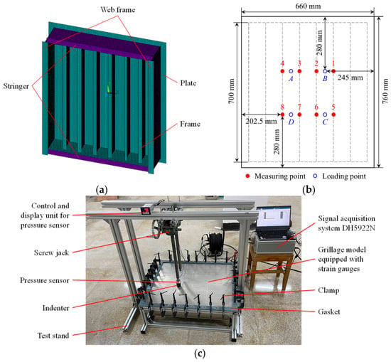
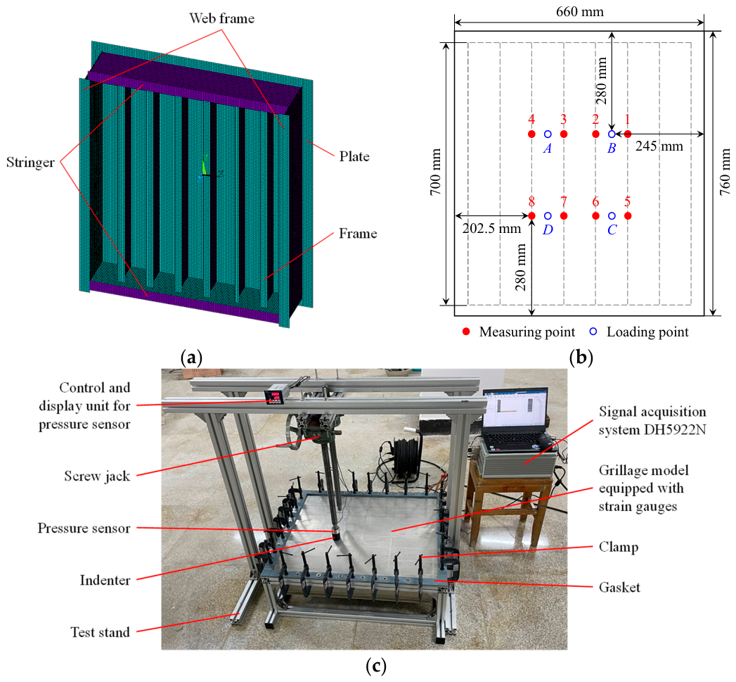
A grillage model is fabricated according to the structural configuration of the bow shoulder of RV Xuelong-2. This model consists of two stringers, six frames, two web frames, and a plate. The dimensions of each component are listed in Table 4. Meanwhile, a 1:1 finite element model (see Figure 14a) is established using 4-node shell elements to construct the influence coefficient matrix.
Table 4.
Component dimensions of the grillage model.
Figure 14.
Physical experiment for the validation of the influence coefficient matrix method. (a) Finite element model of the grillage; (b) locations of measuring and loading points; (c) experimental setup.
Eight strain gauges are mounted on the webs of the central four frames (see Figure 14b). They are placed vertically near the plate (20 mm) to measure normal strains. Four loading points are placed on the plate between frames. Specifically, Measuring Points 1/2, 3/4, 5/6, and 7/8 are used to monitor the loads at Loading Points B, A, C, and D, respectively.
All four boundaries of the model are fixed to a test stand by clamps and gaskets. A screw jack mounted on the stand’s beam is used to apply loads. A pressure sensor is used to measure and record the applied loads. The strain gauges are connected to a signal acquisition system DH5922N in a half-bridge configuration to record the structural responses. The experimental setup for fixing, loading, measurement, and data acquisition described above is depicted in Figure 14c.
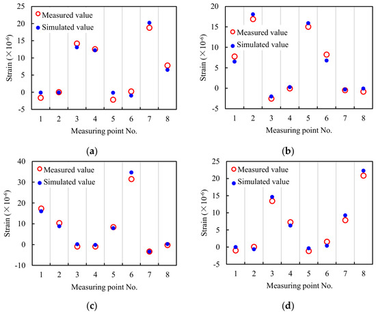
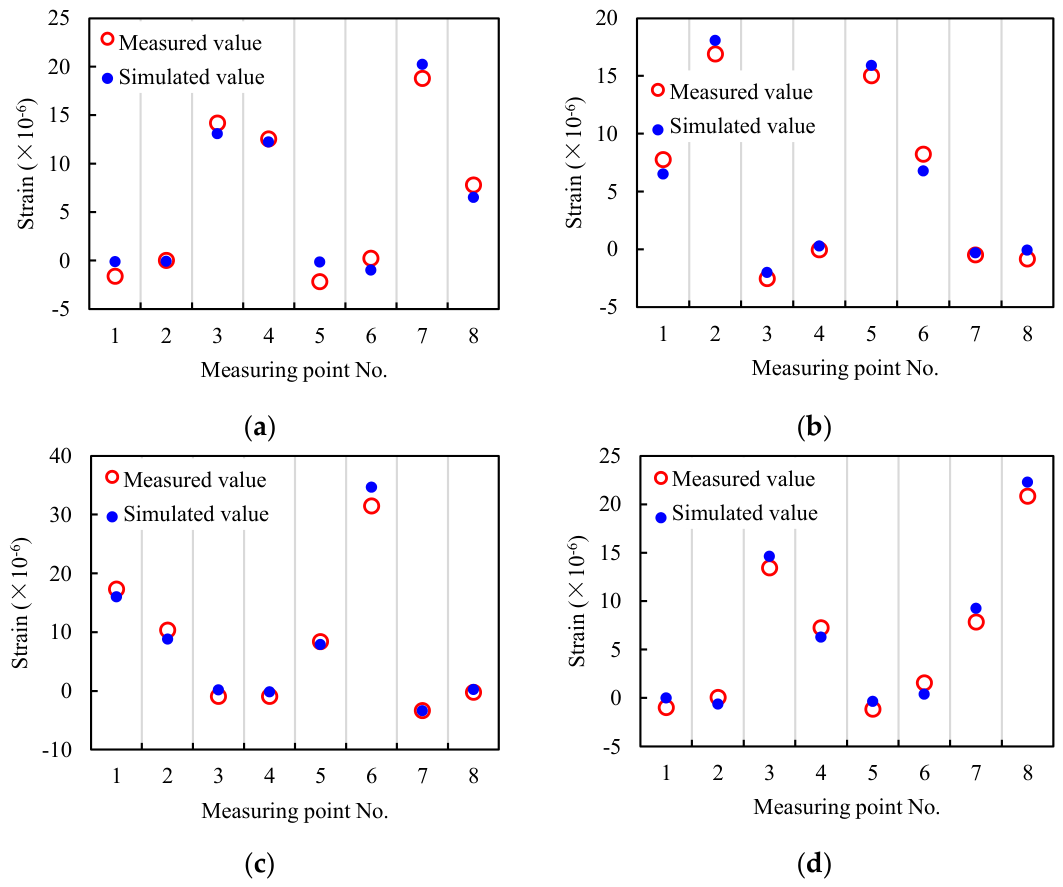
During the experiment, loads of 220.59 N, 204.26 N, 269.53 N, and 225.25 N are sequentially applied at Loading Points A, B, C, and D, corresponding to Cases 1–4, respectively. The above loading cases are simultaneously applied to the finite element model for calibration. As shown in Figure 15, the simulated strain responses are in good agreement with the measured data, validating the consistency of mechanical properties between the finite element model and physical model. Therefore, the former can be used to construct the influence coefficient matrix.
Figure 15.
Comparison between simulated and measured strain responses. (a) Case 1; (b) Case 2; (c) Case 3; (d) Case 4.
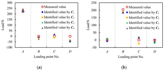
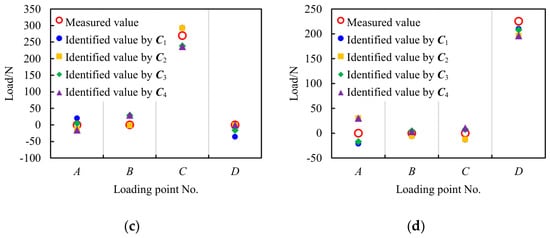
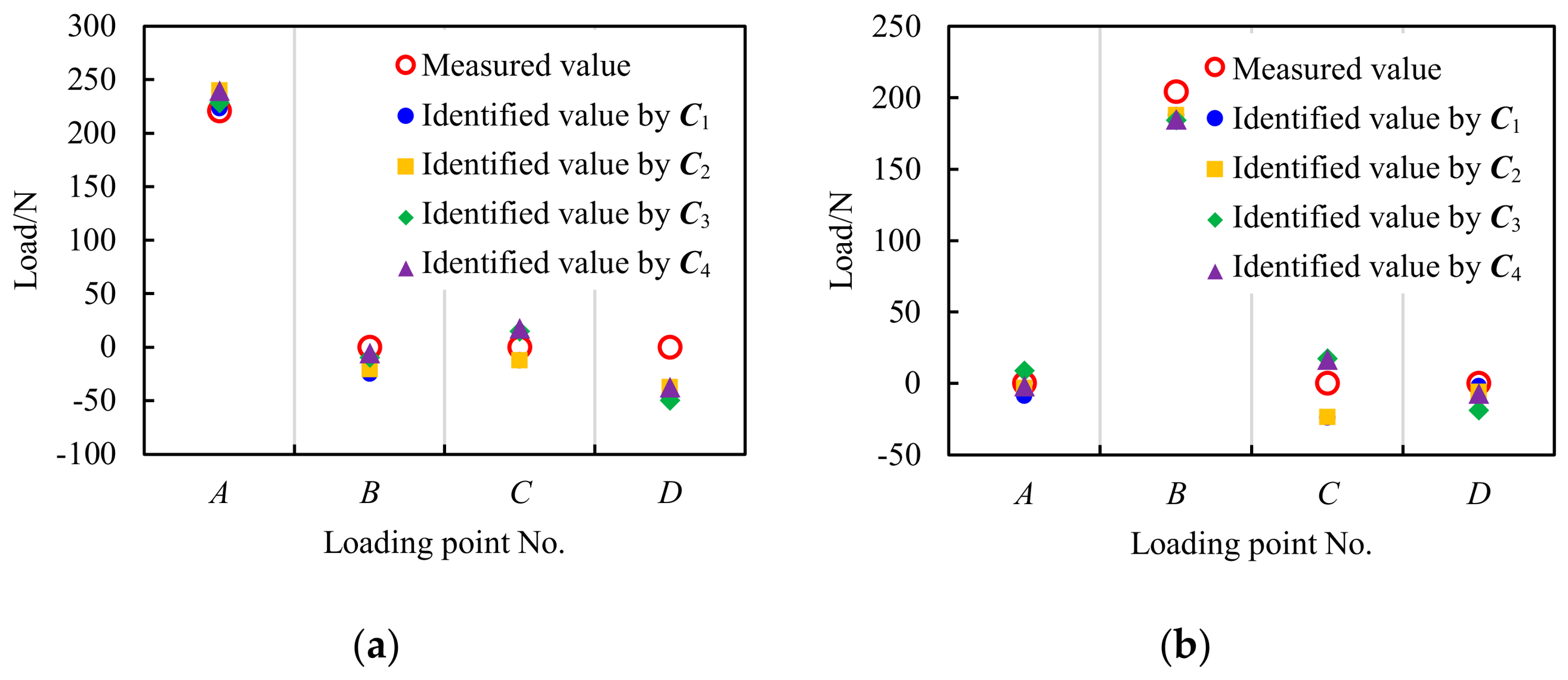
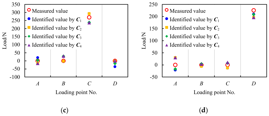
For local ice load identification based on normal strains, a single measuring point is sufficient to monitor the ice load in its corresponding subarea. To fully validate the influence coefficient matrix method, two measuring points are assigned to each loading point in this experiment, thus forming four combinations of loading points and measuring points. Accordingly, four 4th-order influence coefficient matrices are constructed, namely based on Measuring Points 1, 3, 5, 7; based on Measuring Points 1, 4, 5, 8; based on Measuring Points 2, 3, 6, 7; and based on Measuring Points 2, 4, 6, 8. The load values identified by these matrices are compared with the measured values in Figure 16, and the relative errors are listed in Table 5. It can be observed that each matrix achieves satisfactory identification results, with relative errors below 15% in all cases. Therefore, the influence coefficient matrix method is validated to possess a reliable identification capability for local ice loads.
Figure 16.
Comparison between identified and measured load values. (a) Case 1; (b) Case 2; (c) Case 3; (d) Case 4.
Table 5.
Relative errors between identified and measured load values.
4.3. Identification of the Local Ice Loads on RV Xuelong-2
The raw data of ice-induced strains measured on RV Xuelong-2 are processed by the moving average filtering algorithm [13] to reduce noise, according to the following equation:
where denotes the raw data, represents the processed data, and is the moving average window size. This parameter is set to 10 in this study, following the principle of minimizing noise without significantly weakening load peaks.
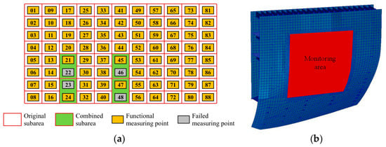
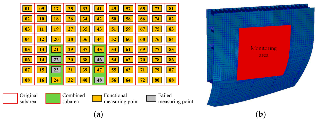
Subsequent examination of the processed data reveals that Measuring Points 22, 23, 46, and 48 were not working properly during the 12th CHINARE-Arctic. The strain signal outputs at these points are consistently null. To reduce the impact of failed measuring points on ice load identification, the monitoring area is redivided by combining the corresponding subareas of the failed point and its neighboring functional point. The effectiveness of this method has been validated in the research by Wang et al. [8]. As depicted in Figure 17a, the number of subareas decreases from 88 to 84. Measuring Points 21, 24, 45, and 47 are used to monitor the ice load in the newly combined subareas.
Figure 17.
Construction of the influence coefficient matrix for identifying the local ice loads on RV Xuelong-2. (a) Redivision of the ice load monitoring area; (b) finite element model of RV Xuelong-2’s bow shoulder.
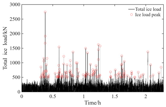
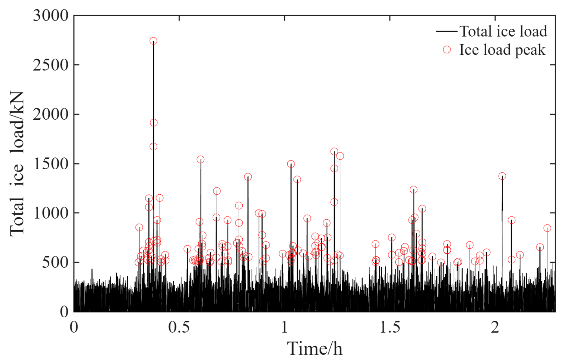
Following the adjusted monitoring scheme, a calibrated finite element model (see Figure 17b) of RV Xuelong-2’s bow shoulder is used to construct an 84th-order influence coefficient matrix. Table 6 lists the model’s parameter settings. The monitoring area and measuring point arrangement are consistent with those on the actual ship. By summing the ice load identified in every subarea using Equation (7), the total ice load (see Figure 18) throughout the monitoring area is obtained.
where denotes the ice load in the corresponding subarea of Measuring Point , is the area of that subarea, , and is the number of subareas.
Table 6.
Parameter settings of the finite element model of RV Xuelong-2’s bow shoulder.
Figure 18.
Identification and peak extraction results of the total ice load throughout the monitoring area of RV Xuelong-2 (5:40–8:00 UTC, 16 August 2021).
In addition to ice impacts, a ship is also subjected to water resistance during an icebreaking process. Although the water-induced strain is small, it will still make a difference to the readings of fiber optic sensors, compromising the purity of the identification results. Therefore, characteristic parameters—especially the peak values and periods of local ice loads—need to be extracted from the identification results for subsequent statistical analysis.
The Rayleigh separation method [42] operates by comparing two neighboring maxima with the minimum value between them. When that minimum value falls below the product of the lower maximum and a separation factor , the load event is separated into two independent peak events. The duration of a peak event is then taken as the time interval between the neighboring minima [43]. In addition, based on the noise level of the measured data during open-water navigation, a threshold is applied to filter out non-ice-induced components from the time history curve.
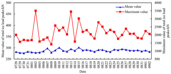
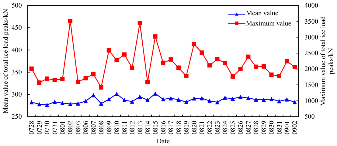
With reference to the parameter settings for other polar ships [34,35,44] and considering the noise level of the measured data during RV Xuelong-2’s open-water navigation, and are set to 0.5 and 50 kN/m, respectively. The peak extraction results of total ice loads are depicted in Figure 18. Based on the strain signal outputs and sea ice images recorded during the 12th CHINARE-Arctic, 902 typical ship–ice interaction cases are selected, from which 1,240,164 peak events of ice loads are extracted. According to the daily fluctuation of total ice load peaks during the voyage in ice-covered waters shown in Figure 19, the mean value shows small variations around 285 kN. In contrast, the maximum value exhibits greater variability. It exceeds 3000 kN on 2 August, 13 August, and 15 August, but drops below 1500 kN on 8 August.
Figure 19.
Daily fluctuation of total ice load peaks on RV Xuelong-2 during the voyage in ice-covered waters.
5. Statistical Analysis of the Relationship Between Ship Speeds, Ice Conditions and the Local Ice Loads on RV Xuelong-2
5.1. Relationship Between Ship Speeds and Local Ice Loads
According to the recognition results of ice parameters, the predominant ice type is pack ice, with concentrations between 0.4 and 0.8 (see Figure 9) and thicknesses below 3.0 m (see Figure 13). The ship speed is generally below 5.0 m/s.
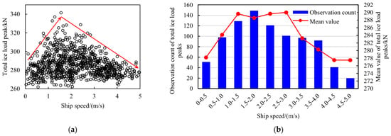
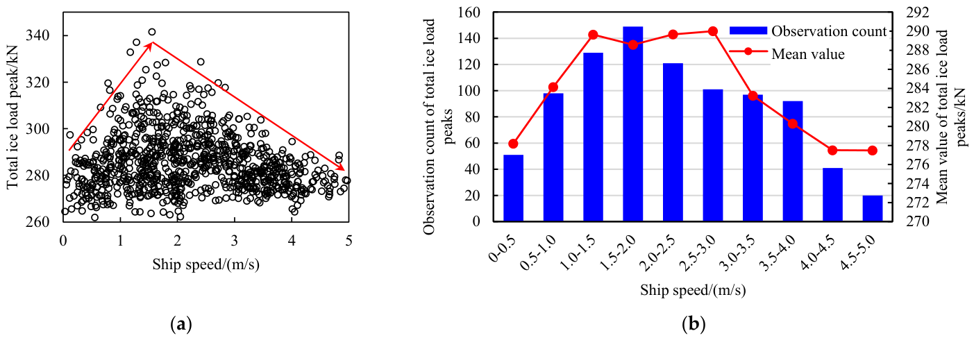
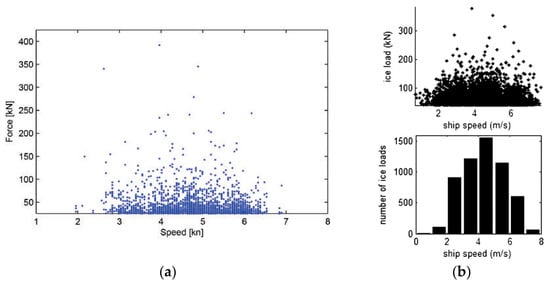
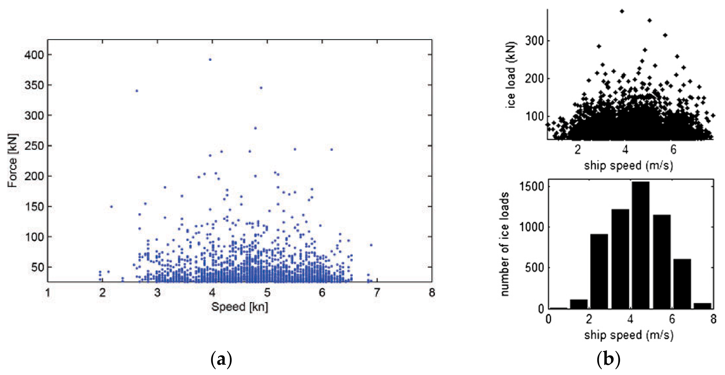
The scatter plot of total ice load peaks with respect to ship speeds under typical ship–ice interaction cases is shown in Figure 20a. To illustrate the relationship more intuitively, the speeds are divided into intervals of 0.5 m/s. The observation counts and mean values of total ice load peaks are statistically analyzed in every speed interval. As depicted in Figure 20b, both mean values and observation counts increase first and then decrease with the rise of ship speeds. The transition range of this trend occurs at 1.0–3.0 m/s. Similar statistical results were reported by Leira et al. [33] and Kotilainen et al. [45] based on the measured data from KV Svalbard and S. A. Agulhas II, as shown in Figure 21.
Figure 20.
Relationship between total ice load peaks and ship speeds under typical ship–ice interaction cases. (a) Scatter plot. (b) Statistical plot.
Figure 21.
Relationship between total ice load peaks and ship speeds for other polar ships. (a) KV Svalbard [33]; (b) S. A. Agulhas II [45].
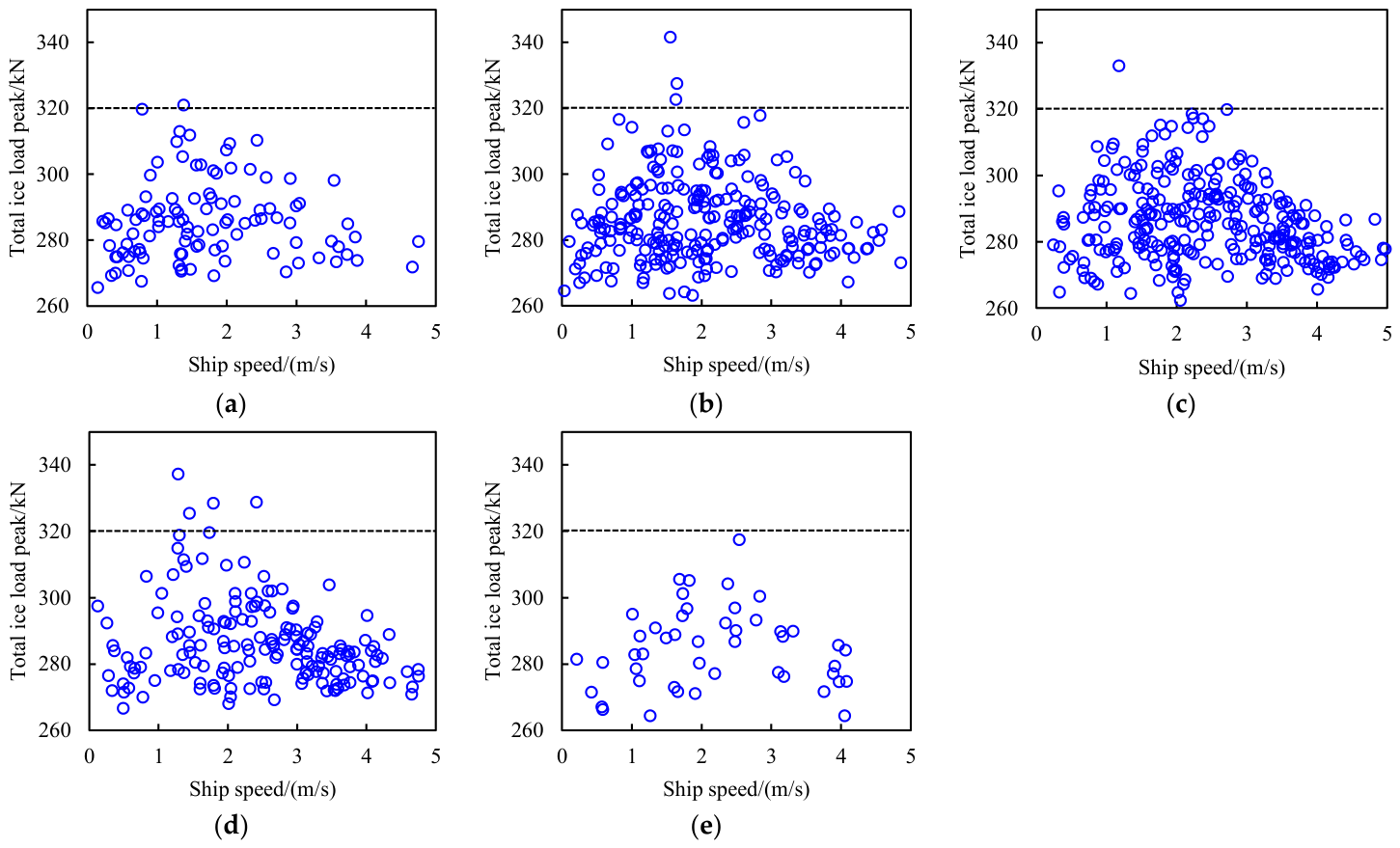
The transition of total ice load peaks may be attributed to the coupling effect between ship speeds and ice parameters. To investigate this, the ice concentration (ci) range of 0.4–0.8 is divided into intervals of 0.1, and the ice thickness (hi) range of 1–2 m is divided into intervals of 0.2 m. The scatter plots of total ice load peaks with respect to ship speeds in each interval are presented in Appendix A. Thus, the ice parameters corresponding to the data points in Figure 20a are determined. It is concluded that the vast majority of total ice load peaks exceeding 320 kN occur when the ship navigates at speeds of 1.0–2.0 m/s under ice conditions of ci = 0.6–0.8 and hi = 1.2–1.8 m. In contrast, the peaks are generally much lower for other combinations of ice thickness, ice concentration, and ship speed. Therefore, the range of 1.0–2.0 m/s can be defined as the “speed of concern” for RV Xuelong-2’s navigation in ice-covered waters. To reduce the likelihood of the ship being subjected to significant ice loads, it is advisable to avoid navigating at the “speed of concern” under the above ice conditions.
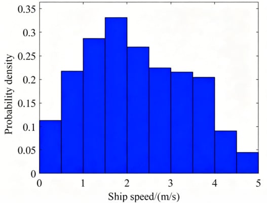
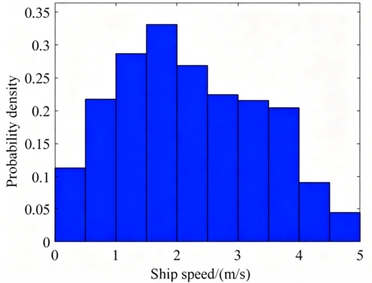
The concept of “exposure” [46], which is expressed in the lay term “the longer you fish, the bigger the fish you catch”, effectively describes how the observation counts of total ice load peaks relate to ship speeds. The probability distribution of ship speeds during the voyage in ice-covered waters is shown in Figure 22. The probability density rises first and then declines, reaching its maximum value in the interval of 1.5–2.0 m/s. A comparison with Figure 20b reveals a high consistency between the two trends. Consequently, speed intervals with higher probability densities yield more ship–ice interaction cases, thereby raising the chance of observing ice load peaks.
Figure 22.
Probability distribution of ship speeds during the voyage in ice-covered waters.
5.2. Relationship Between Ice Concentrations and Local Ice Loads Influenced by Ship Speeds
The strong randomness of ice loads makes it challenging to control variables to study a single factor [13]. Therefore, the analysis in this section is carried out in the mainly distributed range of 1.5 ± 0.5 m to minimize the influence of ice thicknesses.
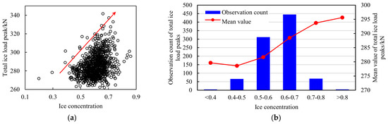
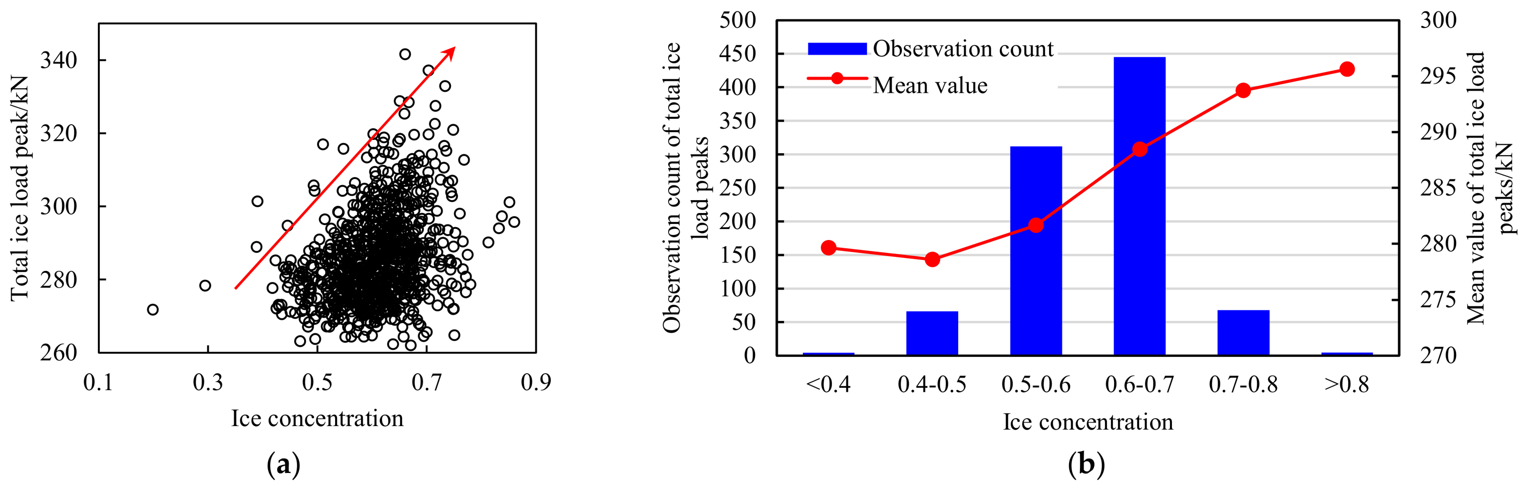
Figure 23a presents a scatter plot of total ice load peaks with respect to ice concentrations under typical ship–ice interaction cases. To illustrate the relationship more intuitively, the concentration is partitioned into 0.1-wide intervals. In each interval, the mean values and observation counts of total ice load peaks are statistically analyzed. As shown in Figure 23b, the mean values increase with rising concentrations, whereas the observation counts first rise and then fall. The latter trend follows the probability distribution of ice concentrations (see Figure 9). According to the “exposure” concept, concentration intervals with higher probability densities involve more ship–ice interaction cases, thus increasing the chance of observing ice load peaks.
Figure 23.
Relationship between total ice load peaks and ice concentrations under typical ship–ice interaction cases. (a) Scatter plot. (b) Statistical plot.
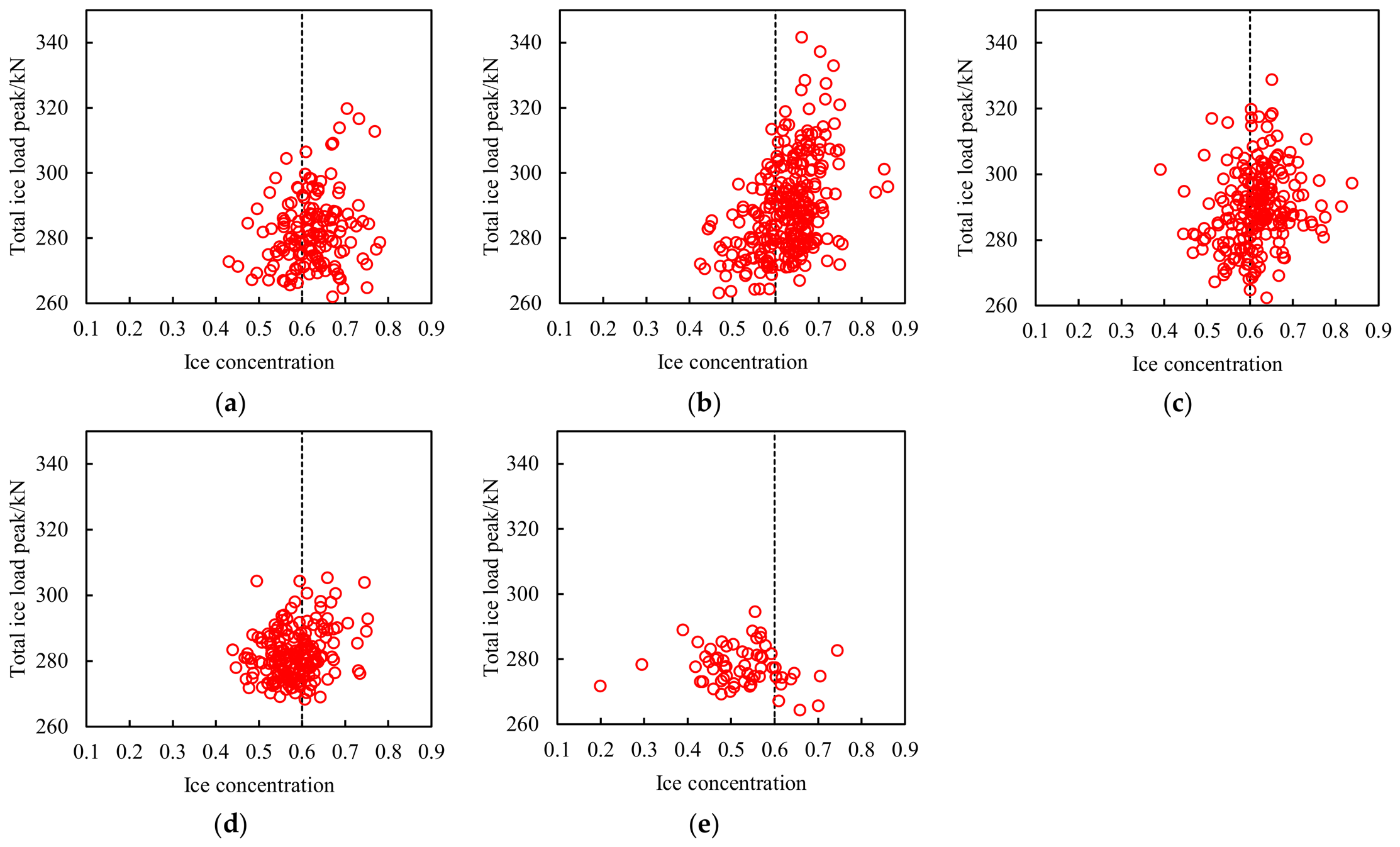
To identify the ship speeds associated with the data points in Figure 23a, the speed range of 0–5.0 m/s is partitioned into 1.0 m/s-wide intervals. Appendix B shows the scatter plots of total ice load peaks versus ice concentrations in different speed intervals. With the increase in ship speeds, the data points gradually move toward smaller ice concentration ranges (from ci > 0.6 to ci < 0.6), along with a notable decrease in the magnitude of total ice load peaks.
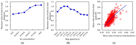
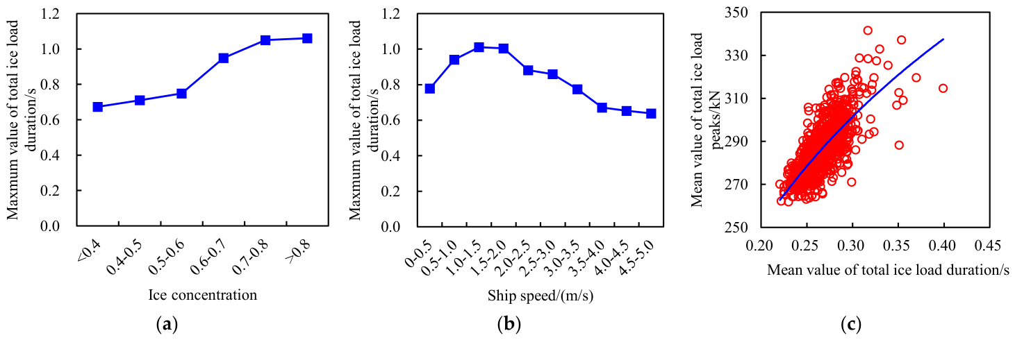
The above trend can be mechanistically explained by the influence of ice concentrations and ship speeds on the duration of ice loads (see Figure 24a,b), along with its correlation to ice load peaks (see Figure 24c). On the one hand, high concentrations restrict the movement of the ice blocks interacting with the hull, thereby lengthening the duration of ice loads and resulting in larger peaks. Conversely, low concentrations allow ice floes to be immediately pushed away upon collision, which significantly shorten the ice load duration and result in smaller peaks. On the other hand, high concentrations increase the obstruction effect on the ship, leading to a passive speed reduction. Under such circumstances, the captain would typically slow down, which further extends the ice load duration and leads to larger peaks.
Figure 24.
Relationship between total ice load duration, ice concentration, ship speed, and total ice load peak. (a) Total ice load duration vs. ice concentration; (b) total ice load duration vs. ship speed; (c) total ice load duration vs. total ice load peak.
5.3. Relationship Between Ice Thicknesses and Local Ice Loads Influenced by Ship Speeds
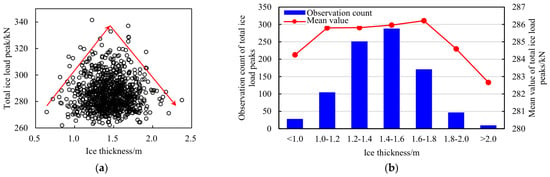
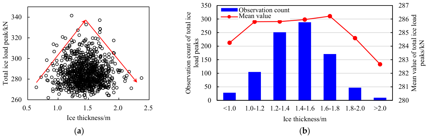
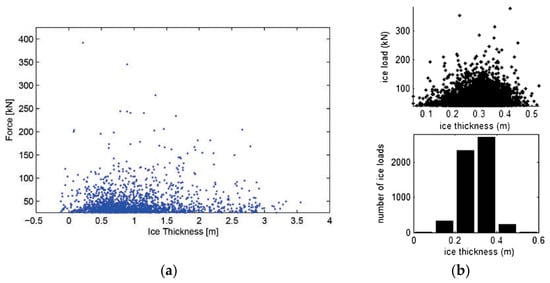
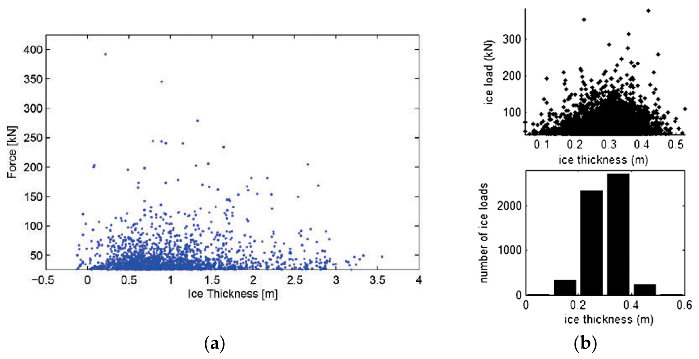
The analysis in this section is carried out in the mainly distributed range of 0.6 ± 0.1 to minimize the impact of ice concentrations. The scatter plot of total ice load peaks with respect to ice thicknesses under typical ship–ice interaction cases is shown in Figure 25a. To illustrate the relationship more intuitively, the thicknesses are divided into intervals of 0.2 m. In every interval, the observation counts and mean values of total ice load peaks are statistically analyzed. As depicted in Figure 25b, both mean values and observation counts increase first and then decrease with the rise of ice thicknesses. The transition range of this trend occurs at 1.0–1.8 m. Similar statistical results were reported by Leira et al. [33] and Kotilainen et al. [45] based on the measured data from KV Svalbard and S. A. Agulhas II, as shown in Figure 26.
Figure 25.
Relationship between total ice load peaks and ice thicknesses under typical ship–ice interaction cases. (a) Scatter plot. (b) Statistical plot.
Figure 26.
Relationship between total ice load peaks and ice thicknesses for other polar ships. (a) KV Svalbard [33]; (b) S. A. Agulhas II [45].
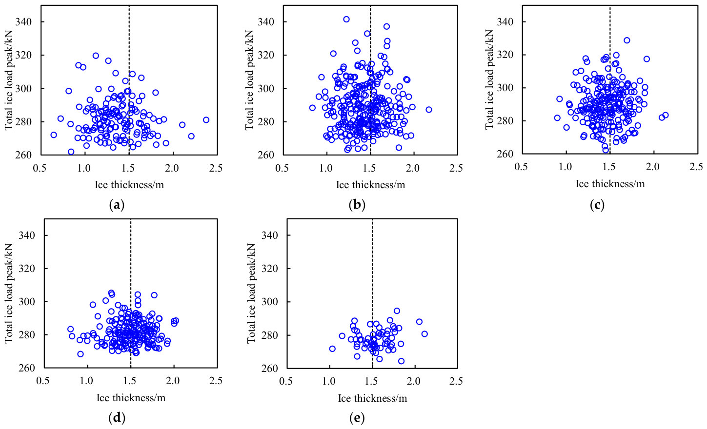
To identify the ship speeds associated with the data points in Figure 25a, the speed range of 0–5.0 m/s is partitioned into 1.0 m/s-wide intervals. Appendix C presents the scatter plots of total ice load peaks versus ice thicknesses in different speed intervals. The data points are symmetrically distributed around hi = 1.5 m. With the increase in ship speeds, the magnitude of total ice load peaks decreases substantially, but the data points do not shift toward lower ice thickness ranges.
This suggests that the correlation between ship speeds and ice thicknesses is weaker than that with ice concentrations. This phenomenon may be attributed to the captain’s limited perception of ice thicknesses from the bridge, whereas the visually prominent ice concentrations serve as the primary reference for speed adjustment. This weak correlation may also explain the discrepancy between the observation counts of total ice load peaks and the probability distribution of ice thicknesses. It is planned to improve the recognition capability of ice parameters for the real-time monitoring system of RV Xuelong-2. The observation images and recognition results of ice parameters will be transmitted in real-time to the bridge to support the decision-making of ship speeds and navigation routes.
The competition between ice failure modes provides a possible mechanism for the relationship between total ice load peaks and ice thicknesses. During an icebreaking process, owing to the difference in hull geometry and the complexity of ice material properties, sea ice exhibits various failure modes, such as bending, crushing, and splitting. The occurrence of one failure mode suppresses/alleviates the presence of other failure modes. Lu et al. [47] proposed a competing mechanism for ice failure modes related to the characteristic length of sea ice. Kong [48] conducted a preliminary study on the relationship between the characteristic length and thickness of sea ice. The transition of total ice load peaks at the ice thickness of around 1.5 m may be attributed to a shift in the dominant ice failure mode at this critical thickness, and the trend of total ice load peaks varies under different failure modes. Currently, research on the competition mechanism of ice failure modes remains at the stage of theoretical analysis. In future expeditions, image data from the ship–ice interaction area will be collected and analyzed to further validate the theory and to investigate the factors influencing the competition between ice failure modes.
6. Conclusions
The field measurement on polar ships serves as a crucial approach for accurately assessing and scientifically understanding ice conditions and local ice loads. In this research, the instrumentation for the field measurement on RV Xuelong-2 is discussed. Ice conditions are recorded by the cameras mounted around the bridge and compass deck, and ice-induced normal strains are measured by the fiber optic sensors deployed on the frames in the bow shoulder area.
A deep convolutional neural network and Hough transform principle are respectively applied to extract ice concentrations and thicknesses from sea ice images. Their distribution along the route, daily fluctuation, and probability distribution during the 12th CHINARE-Arctic are analyzed. Ice concentrations mainly range between 0.4 and 0.8, with relatively high levels near the North Pole and a relatively uniform distribution along other sections of the route. Ice thicknesses are primarily distributed in the range of 0–3.0 m and can be approximated by a lognormal distribution. The distribution along the route is relatively uniform, and no clear increasing trend is exhibited with the rise of latitude.
The influence coefficient matrix method is validated by a physical experiment and applied to identify local ice loads from ice-induced strains. The Rayleigh separation method is applied to extract the peaks and periods of the total ice load throughout the monitoring area. Subsequently, the relationship between ship speeds, ice conditions, and the local ice loads on RV Xuelong-2 is statistically analyzed and mechanistically explained. The coupling effect between ship speeds and ice parameters, along with the competition between ice failure modes, may cause ice load peaks to transition from increasing to decreasing under specific conditions, such as a ship speed of 1.0–3.0 m/s and ice thickness of around 1.5 m. Under high ice concentrations, a prolonged ice load duration—resulting from restricted ice movement and reduced ship speeds—is an important factor contributing to the positive relationship between ice concentrations and ice load peaks. Moreover, intervals of ship speeds and ice concentrations with higher probability densities involve more ship–ice interaction cases, thereby raising the chance of observing ice load peaks.
It should be noted that the “speed of concern” derived from the statistical analysis of a single voyage dataset lacks universality. In future research, continuous and extensive field measurements will be conducted on various ships across different seasons and waters to enhance the diversity and completeness of the dataset. This will help explore the ice load characteristics applicable to a broader range of ships and operational environments. Moreover, the influencing factors of local ice loads and the underlying physical mechanisms will be further investigated and clarified. Appropriate statistical methods or predictive models will be selected to quantify the relationship between local ice loads and their influencing factors, thereby providing necessary support for the safety warning of Arctic navigation.
Author Contributions
Conceptualization, J.W.; methodology, J.W.; validation, J.W.; formal analysis, J.W.; investigation, J.W.; resources, J.W.; data curation, J.W.; writing—original draft preparation, J.W., R.H. and X.L.; writing—review and editing, J.W., R.H. and X.L.; visualization, J.W., R.H. and X.L.; supervision, N.Z. and D.H.; project administration, N.Z. and Q.W.; funding acquisition, J.W. All authors have read and agreed to the published version of the manuscript.
Funding
This research is supported by the National Key Research and Development Program of China (Grant Nos. 2025YFE0214900, 2025YFE0214903), the National Natural Science Foundation of China (Grant Nos. 52501328, 52501329, 52471278, 52192690, 52192695), and the Fundamental Research Funds for the Central Universities (Grant Nos. HEU3072025CFJ0112, HEU3072025PT0103).
Data Availability Statement
The original contributions presented in this study are included in the article. Further inquiries can be directed to the corresponding author.
Acknowledgments
The authors would like to thank the members of the 12th CHINARE-Arctic, and Shunying Ji from Dalian University of Technology, for their support in the field measurement.
Conflicts of Interest
The authors declare no conflicts of interest.
Abbreviations
The following abbreviations are used in this manuscript:
| RV | Research vessel |
| CHINARE-Arctic | Chinese National Arctic Research Expedition |
| DCNN | Deep convolutional neural network |
| CBAM | Convolution block attention module |
| MPA | Mean pixel accuracy |
| IoU | Intersection over union |
| MIoU | Mean intersection over union |
Appendix A
Figure A1.
Scatter plots of total ice load peaks with respect to ship speeds in different ice concentration (ci) intervals. (a) ci = 0.4–0.5; (b) ci = 0.6–0.6; (c) ci = 0.6–0.7; (d) ci = 0.7–0.8.
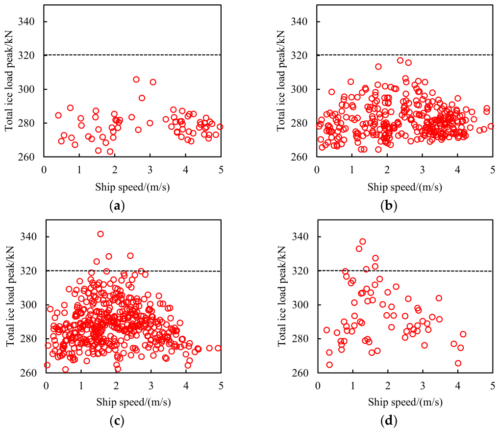
Figure A2.
Scatter plots of total ice load peaks with respect to ship speeds in different ice thickness (hi) intervals. (a) hi = 1.0–1.2 m; (b) hi = 1.2–1.4 m; (c) hi = 1.4–1.6 m; (d) hi = 1.6–1.8 m; (e) hi = 1.8–2.0 m.
Appendix B
Figure A3.
Scatter plots of total ice load peaks with respect to ice concentrations in different ship speed (vs) intervals. (a) vs = 0–1.0 m/s; (b) vs = 1.0–2.0 m/s; (c) vs = 2.0–3.0 m/s; (d) vs = 3.0–4.0 m/s; (e) vs = 4.0–5.0 m/s.
Appendix C
Figure A4.
Scatter plots of total ice load peaks with respect to ice thicknesses in different ship speed (vs) intervals. (a) vs = 0–1.0 m/s; (b) vs = 1.0–2.0 m/s; (c) vs = 2.0–3.0 m/s; (d) vs = 3.0–4.0 m/s; (e) vs = 4.0–5.0 m/s.
References
- Overland, J.; Dunlea, E.; Box, J.; Corell, R.; Forsius, M.; Kattsov, V.; Olseng, M.; Pawlak, J.; Reiersen, L.; Wang, M. The urgency of Arctic change. Polar Sci. 2019, 21, 6–13. [Google Scholar] [CrossRef] [Scilit]
- Lasserre, F.; Cyr, A. Geopolitics and shipping development in the Arctic. Ocean Yearb. Online 2022, 36, 416–439. [Google Scholar] [CrossRef] [Scilit]
- Wang, J.; Duan, Q.; Ji, S. Research progress of field measurements and inversion methods of ice loads on ship structure during ice navigation. Adv. Mech. 2020, 50, 202003. [Google Scholar]
- Böhm, A.; Polach, R.; Herrnring, H.; Ehlers, S. The measurement accuracy of instrumented ship structures under local ice loads using strain gauges. Mar. Struct. 2021, 76, 102919. [Google Scholar] [CrossRef] [Scilit]
- Wu, G.; Kong, S.; Tang, W.; Lei, R.; Ji, S. Statistical analysis of ice loads on ship hull measured during Arctic navigations. Ocean Eng. 2021, 223, 108642. [Google Scholar] [CrossRef] [Scilit]
- Kong, S.; Cui, H.; Wu, G.; Ji, S. Full-scale identification of ice load on ship hull by least square support vector machine method. Appl. Ocean Res. 2021, 106, 102439. [Google Scholar] [CrossRef] [Scilit]
- He, S.; Guo, X.; Chen, X.; Ji, S. Identification of dynamic ice load and full-scale data analysis for ship structures based on Green’s function method. Ocean Eng. 2025, 340, 122333. [Google Scholar] [CrossRef] [Scilit]
- Wang, J.; Chen, X.; Duan, Q.; Ji, S. Eliminating the influence of measuring point failure in ice load identification of polar ship structures. Ocean Eng. 2022, 261, 112082. [Google Scholar] [CrossRef] [Scilit]
- John, J.; Daley, C. Shipboard measurement of ice pressures in the Bering, Chukchi, and Beaufort Seas. In Proceedings of the 3rd International Offshore Mechanics and Arctic Engineering Symposium, New Orleans, LA, USA, 12–17 February 1984. [Google Scholar]
- Kujala, P.; Vuorio, J. Results and Statistical Analysis of Ice Load Measurements on Board Icebreaker Sisu in Winters 1979 to 1985; Research Report No 43; Winter Navigation Research Board: Helsinki, Finland, 1986. [Google Scholar]
- Lee, J.; Kwon, Y.; Rim, C.; Lee, T. Characteristics analysis of local ice load signals in ice-covered water. Int. J. Nav. Archit. Ocean Eng. 2016, 8, 66–72. [Google Scholar] [CrossRef] [Scilit]
- Kujala, P.; Jiang, Z.; Li, F.; Lu, L. Long term prediction of local ice loads on the hull of S. A. Agulhas II. In Proceedings of the 25th International Conference on Port and Ocean Engineering Under Arctic Conditions, Delft, The Netherlands, 9–13 June 2019. [Google Scholar]
- Zhao, G.; Zhao, C.; Xia, X.; Lin, R.; He, S.; Chen, X.; Ji, S. Study of ice load on hull structure based on full-scale measurements in Bohai Sea. J. Mar. Sci. Eng. 2025, 13, 2297. [Google Scholar] [CrossRef] [Scilit]
- Jiang, J.; He, S.; Jiang, H.; Chen, X.; Ji, S. Research on sea ice and local ice load monitoring system for polar cargo vessels. J. Mar. Sci. Eng. 2025, 13, 808. [Google Scholar] [CrossRef] [Scilit]
- Deser, C.; Teng, H. Evolution of Arctic sea ice concentration trends and the role of atmospheric circulation forcing, 1979–2007. Geophys. Res. Lett. 2013, 35, L02504. [Google Scholar] [CrossRef] [Scilit]
- Seymour, W.; Katharine, A.; Andy, L.; Duncan, J. CryoSat-2 estimates of Arctic sea ice thickness and volume. Geophys. Res. Lett. 2013, 40, 732–737. [Google Scholar]
- Yan, Q.; Huang, W. Detecting sea ice from techDemoSat-1 data using support vector machines with feature selection. IEEE J. Sel. Top. Appl. Earth Obs. Remote Sens. 2019, 12, 1409–1416. [Google Scholar] [CrossRef] [Scilit]
- Aldenhoff, W.; Berg, A.; Eriksson, L. Sea ice concentration estimation from Sentinel-1 Synthetic Aperture Radar images over the Fram Strait. In Proceedings of the 36th IEEE International Geoscience and Remote Sensing Symposium, Beijing, China, 10–15 July 2016. [Google Scholar]
- Han, H.; Hong, S.; Kim, H.; Chae, T.; Choi, H. A study of the feasibility of using KOMPSAT-5 SAR data to map sea ice in the Chukchi Sea in late summer. Remote Sens. Lett. 2017, 8, 468–477. [Google Scholar] [CrossRef] [Scilit]
- Barbat, M.; Wesche, C.; Werhli, A.; Mata, M. An adaptive machine learning approach to improve automatic iceberg detection from SAR images. ISPRS J. Photogramm. Remote Sens. 2019, 156, 247–259. [Google Scholar] [CrossRef] [Scilit]
- Wang, Q.; Lu, P.; Zu, Y.; Li, Z.; Leppäranta, M.; Zhang, G. Comparison of passive microwave data with shipborne photographic observations of summer sea ice concentration along an Arctic cruise path. Remote Sens. 2019, 11, 2009. [Google Scholar] [CrossRef] [Scilit]
- Wang, J.; Wang, Y.; Wang, Q.; Xue, Y.; Han, D. Far-field identification and statistical analysis of ice loads measured on polar ships in the Arctic region. Ocean Eng. 2025, 340, 122418. [Google Scholar] [CrossRef] [Scilit]
- Weissling, B.; Ackley, S.; Wagner, P.; Xie, H. EISCAM-Digital image acquisition and processing for sea ice parameters from ships. Cold Reg. Sci. Technol. 2009, 57, 49–60. [Google Scholar] [CrossRef] [Scilit]
- Amouzadrad, P.; Mohapatra, S.; Guedes Soares, C. Review on sensitivity and uncertainty analysis of hydrodynamic and hydroelastic responses of floating offshore structures. J. Mar. Sci. Eng. 2025, 13, 1015. [Google Scholar] [CrossRef] [Scilit]
- Kalke, H.; Loewen, M. Support vector machine learning applied to digital images of river ice conditions. Cold Reg. Sci. Technol. 2018, 155, 225–236. [Google Scholar] [CrossRef] [Scilit]
- Kim, D.; Nam, J. Determination of the lower boundary of a rotating ice patch for ice thickness estimation using image convolution and machine learning. Cold Reg. Sci. Technol. 2020, 173, 103009. [Google Scholar] [CrossRef] [Scilit]
- Chi, J.; Kim, H. Prediction of Arctic sea ice concentration using a fully data driven deep neural network. Remote Sens. 2017, 9, 1305. [Google Scholar] [CrossRef] [Scilit]
- Zhang, C.; Chen, X.; Ji, S. Semantic image segmentation for sea ice parameters recognition using deep convolutional neural networks. Int. J. Appl. Earth Obs. Geoinform. 2022, 112, 102885. [Google Scholar] [CrossRef] [Scilit]
- Uto, S.; Oka, S.; Murakami, C.; Takimoto, T.; Izumiyama, K. Ice load exerted on the hull of icebreaker PM Teshio in the South Sea of Okhotsk. In Proceedings of the 18th International Conference on Port and Ocean Engineering Under Arctic Conditions, Potsdam, NY, USA, 26–30 June 2005. [Google Scholar]
- Frederking, R. Ice loading on a ship in discontinuous ice. In Proceedings of the 20th International Offshore and Polar Engineering Conference, Beijing, China, 20–25 June 2010. [Google Scholar]
- Hänninen, S.; Lens, M.; Riska, K. Analysis of the Ice Load Measurements During USCGC Healy Ice Trials, Spring 2000; Report M-265; Helsinki University of Technology, Ship Laboratory: Espoo, Finland, 2001. [Google Scholar]
- Frederking, R. Local Ice Pressures from the Louis S. St. Laurent 1994 North Pole Transit; Technical Report HYD-TR-054; Canadian Hydraulics Centre; National Research Council of Canada: Ottawa, ON, Canada, 2000.
- Leira, B.; Børsheim, L.; Espeland, Ø.; Amdahl, J. Ice-load estimation for a ship hull based on continuous response monitoring. Proc. Inst. Mech. Eng. Part M—J. Eng. Marit. Environ. 2009, 223, 529–540. [Google Scholar] [CrossRef] [Scilit]
- Suyuthi, A.; Leira, B.; Riska, K. Short term extreme statistics of local ice loads on ship hulls. Cold Reg. Sci. Technol. 2012, 82, 130–143. [Google Scholar] [CrossRef] [Scilit]
- Suominen, M.; Kujala, P.; Romanoff, J.; Remes, H. Influence of load length on short-term ice load statistics in full-scale. Mar. Struct. 2017, 52, 153–172. [Google Scholar] [CrossRef] [Scilit]
- Jeon, M.; Choi, K.; Min, J.; Ha, J. Estimation of local ice load by analyzing shear strain data from the IBRV Araon’s 2016 Arctic voyage. Int. J. Nav. Archit. Ocean Eng. 2018, 10, 421–425. [Google Scholar] [CrossRef] [Scilit]
- Wang, J.; Chen, X.; Sun, K.; Ji, S. Far-field identification of ice loads on ship structures by radial basis function neural network. Ocean Eng. 2023, 282, 115072. [Google Scholar] [CrossRef] [Scilit]
- Iyerusalimskiy, A.; Choi, J.; Park, G.; Kim, Y.; Yu, H.; John, J. The interim results of the long-term ice loads monitoring on the large Arctic tanker. In Proceedings of the 21st International Conference on Port and Ocean Engineering Under Arctic Conditions, Montreal, QC, Canada, 10–14 July 2011. [Google Scholar]
- Yu, H.; Iyerusalimskiy, A.; Kim, Y.; John, J. Hull structural performance monitoring system for ships operating in ice-covered waters. In Proceedings of the Arctic Technology Conference, Houston, TX, USA, 3–5 December 2012. [Google Scholar]
- Lu, P.; Li, Z. A method of obtaining ice concentration and floe size from shipboard oblique sea ice images. IEEE Trans. Geosci. Remote Sens. 2010, 48, 2771–2780. [Google Scholar]
- Zhang, P.; Chen, X.; Kong, S.; Ji, S.P.; Ji, S.Y. Sea ice thickness identification method based on Hough transform principle. Haiyang Xuebao 2022, 44, 161–169. [Google Scholar]
- Kujala, P.; Suominen, M.; Riska, K. Statistics of ice loads measured on MT Uikku in the Baltic. In Proceedings of the 20th International Conference on Port and Ocean Engineering Under Arctic Conditions, Lulea, Sweden, 9–12 June 2009. [Google Scholar]
- Suominen, M.; Li, F.; Lu, L.; Kujala, P.; Bekker, A.; Lehtiranta, J. Effect of maneuvering on ice-induced loading on ship hull: Dedicated full-scale tests in the Baltic Sea. J. Mar. Sci. Eng. 2020, 8, 759. [Google Scholar] [CrossRef] [Scilit]
- Suominen, M.; Kujala, P. Analysis of Short-Term Ice Load Measurements on Board MS Kemira During the Winters 1987 and 1988; Report AALTO-AM-22; Aalto University, School of Science and Technology: Espoo, Finland, 2010. [Google Scholar]
- Kotilainen, M.; Vanhatalo, J.; Suominen, M.; Kujala, P. Predicting ice-induced load amplitudes on ship bow conditional on ice thickness and ship speed in the Baltic Sea. Cold Reg. Sci. Technol. 2017, 135, 116–126. [Google Scholar] [CrossRef] [Scilit]
- Jordaan, I.; Bruce, J.; Masterson, D.; Frederking, R. Local ice pressures for multiyear ice accounting for exposure. Ocean Eng. 2010, 61, 97–106. [Google Scholar] [CrossRef] [Scilit]
- Lu, W.; Lubbad, R.; Løset, S. Fracture of an ice floe: Local out-of-plane flexural failures versus global in-plane splitting failure. Cold Reg. Sci. Technol. 2016, 123, 1–13. [Google Scholar] [CrossRef] [Scilit]
- Kong, S. Discrete Element Analysis and Monitoring Identification Method of Ice Loads on Ship Structures. Ph.D. Thesis, Dalian University of Technology, Dalian, China, 2020. [Google Scholar]

Disclaimer/Publisher’s Note: The statements, opinions and data contained in all publications are solely those of the individual author(s) and contributor(s) and not of MDPI and/or the editor(s). MDPI and/or the editor(s) disclaim responsibility for any injury to people or property resulting from any ideas, methods, instructions or products referred to in the content. |
© 2026 by the authors. Licensee MDPI, Basel, Switzerland. This article is an open access article distributed under the terms and conditions of the Creative Commons Attribution (CC BY) license.