Theory of Ships Viewed as Slightly Submerged Bodies: A Simple Explanation and Integral Equation Variants

Abstract

The classical Neumann–Kelvin (NK) theory of potential flow around a free-surface-piercing ship that steadily advances in calm water or through regular waves is considered. Specifically, this study presents an elementary ‘no-equation interpretation’ of the rigid-waterplane linear flow model and the related modification of the NK theory recently presented by the authors and complements the detailed mathematical analysis given in that earlier study. Specifically, the NN (Neumann–Noblesse) integral equation obtained in that previous study by applying Green’s fundamental identity to an alternative linear flow model called the rigid-waterplane flow model, in which an open free-surface-piercing ship hull is closed by a rigid waterplane slightly submerged under the free surface, is interpreted in light of Saint-Venant’s principle. Briefly, the present study argues that the NK integral equation obtained in the classical NK theory of potential flow around a ship contains a singularity at the ship waterline and that this singularity is removed—in the spirit of the classical Saint-Venant principle—in the rigid-waterplane flow model and the related weakly-singular NN integral equation, which can then be viewed as a ‘regularization’ of the NK integral equation. This study also presents variants of the NN integral equation in which a function defined in terms of the ship hull surface geometry by an integral over the ship waterplane or an integral around the ship waterline is expressed as equivalent integrals over the ship hull surface. Like the NN integral equation given previously, the equivalent variants of the weakly-singular NN integral equation obtained in this study do not involve a waterline integral and hold for a ship that steadily advances in calm water or through regular waves, as well as for an offshore structure or a moored ship in regular waves.

1. Continuum Mechanics Is Based on Judicious Approximations

The paramount importance of practical computational tools for the hydrodynamic and structural analyses that are required to design ships and offshore structures is well understood and is emphasized in [1]. It is also well understood, although occasionally insufficiently appreciated, that these ‘design tools’ rely on mathematical models and theories that are based on various judicious assumptions and approximations. Examples are well known and numerous, and a few of the best-known and most important theories in solid and fluid mechanics are briefly cited in this introduction.

The structural analysis of ships and offshore structures largely relies on the theory of elasticity developed by Hooke (1678), who laid its foundation with his stress–strain law, Cauchy (1820), who introduced the stress tensor and governing equations, and Navier (1821), Lamé (1852) and Saint-Venant (1855), who made further fundamental contributions. Beam theory, initiated by Galilei in the 17th century, was developed by Euler and Bernoulli (1750) and refined by Timoshenko (1921). Plate theory, which extends the Euler–Bernoulli beam theory to two-dimensional bending, is based on approximations and mathematical models developed by Cauchy (1827), Lamé (1831), Kirchhoff (1850) and Love (1888). Thick-plate theory was developed by Reissner (1945) and Mindlin (1945).

Fluid mechanics arguably is even more complicated than solid mechanics and thus offers a particularly rich set of theories based on various insightful approximations. In particular, the fundamental decomposition of the drag of a ship that steadily advances in calm water into wave-making and viscous-friction components tied to gravity or water viscosity was explained by Froude in the late 1860s and early 1870s. The analysis of wave diffraction–radiation by ships and offshore structures is mostly based on the potential flow theory developed by Euler (1755), who first introduced the velocity potential and governing equations for inviscid and irrotational flows, d’Alembert (1752) and Laplace (1799). The door to practical applications of potential flow theory to bodies such as ships and offshore structures was opened by Green (1828), although Green’s crucial contribution was ignored until Kelvin rediscovered it in the 1840s. Practical methods, based on thin-ship or slender-ship approximations, for predicting the wave drag of a ship were proposed by Michell (1898) and Hogner (1932). Prandtl (1904) offered a practical theory for evaluating viscous effects for flows around streamlined bodies at high Reynolds numbers. Many other theories, based on various judicious assumptions, have been offered, e.g., the Kutta–Joukowski condition at a wing’s sharp trailing edge (1902–1906) and Prandtl’s lifting line theory (1918).

As was already noted, the seminal theories cited in the foregoing are based on judicious assumptions and approximations, as is well understood yet occasionally forgotten. This general rule holds for wave diffraction–radiation by a ship that advances at a constant speed along a straight path in calm water or through regular waves, which is considered in this study. In particular, the theories of the wave-making drag of a ship in calm water proposed by Michell [2] in 1898 and Hogner [3] in 1932 explicitly determine the wave drag of a ship in terms of the length and the speed of the ship and the shape of the ship hull. Despite their remarkable simplicity, these theories have been found to be quite useful. Indeed, Michell’s thin-ship theory has been extensively applied in ship design. Hogner’s theory, although less well known, has also been widely applied, notably to ship hull form optimization [4], to analyze the influence of wave interferences on the far-field wave pattern created by a ship that steadily advances in calm water [5,6,7,8], and to filter unrealistic and inconsequential short ship waves [9,10]. Nevertheless, the approximations underlying Michell’s and Hogner’s theories are overly restrictive for many practical applications, and a more accurate theory—commonly called Neumann–Kelvin (NK) theory—has been considered by Brard [11] and Guevel [12] and in numerous subsequent studies, notably [13,14,15,16,17,18,19,20,21,22,23,24,25,26,27,28].

2. The Neumann–Kelvin Theory of Ship Waves: A 55-Year-Old Puzzle

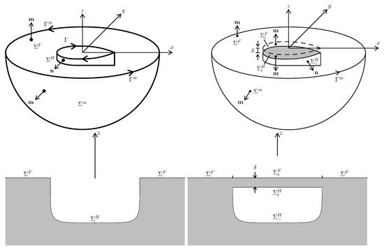
Potential flow theory is realistic for wave diffraction–radiation by large bodies such as ships (and offshore structures), and this basic theoretical framework is widely adopted. Moreover, the boundary condition at the free surface is commonly linearized based on the assumption that the velocity of the flow created by a ship is much smaller than the ship speed, as was first done by Kelvin [29] and Michell [2] in their seminal studies of ship waves. The classical theoretical framework based on potential flow theory and the Kelvin–Michell linear free-surface boundary condition leads to a boundary value problem that consists in solving the Laplace equation in the undisturbed flow region outside the mean wetted hull surface ${\Sigma }^H$ of the ship with a Neumann boundary condition at ${\Sigma }^H,$ where the normal components of the rigid surface ${\Sigma }^H$ and the flow velocity are equal, and the Kelvin–Michell linear free-surface boundary condition at the undisturbed free surface ${\Sigma }^F$ outside ${\Sigma }^H.$ The body surface ${\Sigma }^H$ and the free surface ${\Sigma }^F$ in this classical boundary value problem, widely known as the Neumann–Kelvin (NK) problem, are depicted on the left side of Figure 1. Application of Green’s fundamental identity to the flow potential $\phi$ and the Green function G that satisfies the Kelvin–Michell linear free-surface boundary condition leads to an integral equation, called the NK integral equation hereafter, that determines $\phi$ at the body surface ${\Sigma }^H,$ as is shown in [30,31] and other studies.

Figure 1. The bottom row shows 2D cuts of the 3D flow regions, defined in the top row, that are considered in the classical Neumann–Kelvin (NK) or the rigid-waterplane (RW) linear flow models in the left and right columns.

The NK integral equation is suited for reliable numerical computations in the special case of wave diffraction–radiation by a stationary body such as an offshore structure or a moored ship. However, for a ship that steadily advances in calm water or through waves, the NK integral equation contains a line integral around the ship waterline that was unexpected. Indeed, this waterline integral is puzzling because the contribution of the free surface ${\Sigma }^F$ is expected to vanish if the Green function that satisfies the boundary condition at ${\Sigma }^F$ is used, as is the case for wave diffraction–radiation by a stationary body, and the appearance of a line integral around the ship waterline was the object of intense discussions by members of the International Towing Tank Committee (ITTC) when the NK theory was first considered nearly 55 years ago and has remained a puzzle since.

The NK waterline integral, which does not appear in the special case of a stationary body, as was already noted, has been found to cause major difficulties in numerous numerical applications of the NK theory. These difficulties are summarized in [20] as follows: “The Neumann-Kelvin theory, as it is currently understood, does not give satisfactory wave resistance results for realistic ship hull forms. These results lead to, and reinforce, the suggestion that the problem lies with the waterline integral term; a new treatment of this term may substantially increase the applicability of Neumann-Kelvin theory”. Further evidence of considerable difficulties related to the troublesome waterline integral in the NK integral equation is given in [22], where alternative conjectures about the behavior of the flow potential at a ship waterline are considered, and in [25], where the NK integral equation is shown to yield an ill-conditioned matrix of influence coefficients. Numerous other numerical implementations of the NK theory for a ship that advances in calm water or through waves further illustrate the numerical complexities and uncertainties that stem from the ship waterline integral in the classical NK theory. A partial list of numerical studies of the NK theory is given at the end of the previous section.

3. Origin of the Numerical Difficulties in the NK Theory

As is noted in [30,31], the numerical difficulties observed in the applications of the NK theory reported in [20,22,25] and other studies are most likely related to a fundamental mathematical issue. Specifically, the Kelvin–Michell linear free-surface boundary condition applied at the undisturbed free surface ${\Sigma }^F$ is merely an approximation, as is emphasized in [32], and there is no reason to expect that this linear boundary condition, the Neumann boundary condition at the mean wetted ship hull surface ${\Sigma }^H,$ and the Laplace equation in the undisturbed flow region bounded by ${\Sigma }^H$ and ${\Sigma }^F$ define a smooth flow potential at the ship waterline $\mathsf{\Gamma }$. Thus, the possibility that the flow potential determined by the NK linear flow model is singular along the ship waterline cannot be ruled out and indeed is highly likely. In this thesis, an integral equation that involves the flow potential $\phi$ at the ship waterline $\mathsf{\Gamma }$ cannot be expected to be well suited for reliable numerical solution. Indeed, there is considerable evidence that the difficulties experienced in numerical solutions of the NK integral equation stem from the fact that this theory defines a flow potential $\phi$ that is singular at the ship waterline $\mathsf{\Gamma }.$

In particular, integral equations that do not involve $\phi$ at $\mathsf{\Gamma }$ can be solved without difficulty. Specifically, neither the NK integral equation for wave diffraction–radiation by an offshore structure [33,34] nor the Neumann–Michell (NM) integral equation in the NM theory of potential flow around a ship that steadily advances in calm water [35] involves the flow potential $\phi$ at the waterline $\mathsf{\Gamma }$ of the body (offshore structure or ship) and both these integral equations can be solved without difficulty. Indeed, the NK integral equation for wave diffraction–radiation by an offshore structure is the basis of widely used commercial software, and the NM integral equation for a ship that steadily advances in calm water has been extensively applied [35,36,37,38,39,40,41,42], notably for ship hull form optimization [43,44,45,46,47,48,49,50].

Further supportive evidence for the thesis that the difficulties experienced in numerical solutions of the NK integral equation for a ship that advances in calm water or through waves stem from a singularity of the flow potential $\phi$ at the ship waterline $\mathsf{\Gamma }$ can be found in numerical applications of the NK integral equation reported in the literature. Specifically, numerical solutions of the NK integral equation within the context of a low-order panel method yield realistic predictions if the flow potential ${\phi }^{\mathsf{\Gamma }}$ at the waterline $\mathsf{\Gamma }$ is assumed to be a continuous extension of the potential $\phi$ at the ship hull surface ${\Sigma }^H$ in the vicinity of $\mathsf{\Gamma }$, e.g., if ${\phi }^{\mathsf{\Gamma }}$ at the mid-point of a waterline segment is presumed to be equal to $\phi$ at the centroid of the hull surface panel that contains the waterline segment, as is done in [12,13,14]. Alternatives to this approach consist in applying the waterline integral in the NK integral equation at a small distance below the actual waterline $\mathsf{\Gamma },$ or in merely ignoring it, as is done in [27,28]. These expedient numerical implementations effectively circumvent the difficulties related to a singularity of the flow potential ${\phi }^{\mathsf{\Gamma }}$ at a ship waterline $\mathsf{\Gamma }$ in the NK integral equation. However, attempts to obtain numerical solutions in which the flow potential ${\phi }^{\mathsf{\Gamma }}$ at the ship waterline $\mathsf{\Gamma }$ is determined from a rigorous solution of the NK boundary integral equation in which ${\phi }^{\mathsf{\Gamma }}$ is unconstrained, rather than presumed to be a continuous extension of the potential $\phi$ at the ship hull surface ${\Sigma }^H$ in the vicinity of the ship waterline, result in numerical difficulties, as evidenced in [22,25,26].

Thus, the various numerical studies listed in this section provide strong supportive evidence for the thesis that the numerical difficulties related to the waterline integral in the NK integral equation most likely stem from the fact that this integral equation defines a flow potential $\phi$ that is singular at the waterline of a ship that steadily advances through waves or in calm water.

4. A Way to Avoid the Numerical Difficulties in the NK Theory

The thesis expounded in the previous section also suggests that the numerical difficulties and uncertainties associated with the NK integral equation should not occur for an integral equation that does not involve the flow potential ${\phi }^{\mathsf{\Gamma }}$ at the ship waterline $\mathsf{\Gamma }$ and that such an integral equation would then be well suited for reliable numerical solution. To this end, an alternative flow model to the classical NK linear flow model is considered in [30,31,51]. In this alternative linear flow model, an open free-surface-piercing ship is viewed as the zero-submergence limit of a corresponding closed body that is submerged at an infinitesimally small depth $0<\delta \ll 1$ under the undisturbed free-surface plane, as is illustrated on the right side of Figure 1. This alternative linear flow model is called the rigid-waterplane (RW) flow model in [30,31,51]. In the zero-submergence limit $\delta =0,$ the flow regions defined in the classical NK flow model and the corresponding RW flow model are identical, and both the NK and RW models are then acceptable, and essentially equivalent, linear flow models. However, these alternative linear flow models differ in some respects, as is now explained.

In the classic NK theory, Green’s basic identity is applied in the NK flow region defined on the left side of Figure 1, which can be viewed as the zero-submergence limit $\delta =0$ of the flow region considered in the RW flow model, as was already noted. However, Green’s identity is applied in the $0<\delta \ll 1$ flow region defined on the right side of Figure 1, and the limit $\delta \to 0$ of the corresponding integral equation is subsequently considered in the RW model. Thus, the limit $\delta =0$ is interchanged in the tasks ‘consider a flow region’ and ‘apply Green’s identity in that flow region’ in the NK and RW flow models and the analysis given in [30]. It is also noted in that study that the ship waterline $\mathsf{\Gamma }$ is the intersection curve of two surfaces, the free surface ${\Sigma }^F$ and the mean wetted ship hull surface ${\Sigma }^H,$ in the NK flow model, where the Kelvin–Michell linear free-surface boundary condition or the Neumann hull surface boundary condition are applied. However, in the RW flow model, the waterline $\mathsf{\Gamma }$ separates three surfaces, the free surface ${\Sigma }^F$, the ship hull surface ${\Sigma }^H$ and the ship waterplane ${\Sigma }_i^F$, where three different boundary conditions hold: the free-surface condition, the ship hull surface condition, and a ‘dead-water condition’.

For a small submergence $\delta \ll 1,$ the RW linear flow model allows a flow above the rigid waterplane ${\Sigma }_i^H$ that closes the open ship hull surface ${\Sigma }^H.$ Such a flow within an infinitesimally thin layer of water above the rigid waterplane ${\Sigma }_i^H$ does not have a meaningful global effect on the flow around the ship hull ${\Sigma }^H$ but can have a large, possibly profound, local influence along the ship waterline. This distinction between a negligible global influence and a large local influence is crucial and was beautifully explained in 1855 by Saint-Venant [52,53] in his famous principle, which essentially states that local singularities have limited practical influence on global effects. However, the flow potentials defined by applying Green’s basic identity in the flow regions considered in the classical NK theory or the alternative RW flow model can be expected to greatly differ along the ship waterline $\mathsf{\Gamma }.$

Thus, the RW linear flow model opens a door to the possibility that a particular ‘lucky’ assumption or restriction imposed upon the flow in the thin water layer above the rigid waterplane ${\Sigma }_i^H$ might yield an integral equation that does not involve the flow potential $\phi$ at the ship waterline $\mathsf{\Gamma }$. Three particular assumptions about the flow above ${\Sigma }_i^H$ are examined in [30]. Specifically: (i) no restriction is imposed on that flow, (ii) the flow is assumed to be two-dimensional, and (iii) the thin water layer above ${\Sigma }_i^H$ is assumed to be a ‘dead-water’ region where no flow is allowed. Application of Green’s basic identity to these three variations of the RW linear flow model yields four interesting alternative integral equations [30]. Three of these four integral equations, as well as the NK integral equation related to the classical NK flow model, involve the flow potential ${\phi }^{\mathsf{\Gamma }}$ at the ship waterline $\mathsf{\Gamma }$, but the integral equation that corresponds to the ‘dead-water’ assumption does not.

Thus, the RW flow model with a ‘no-flow’ (dead-water) restriction above the rigid waterplane ${\Sigma }_i^H$ yields an integral equation that stands out in an important respect because this integral equation does not involve the flow potential at the ship waterline, a defining characteristic feature that ensures that this integral equation is well suited for reliable numerical solution via a typical low-order panel method [30].

This ‘standout’ integral equation is identical to the weakly-singular integral equation that was obtained (over forty years ago) in [33]—for the special case of a stationary body (offshore structure or moored ship) and via an analysis based on the classic NK linear flow model rather than the alternative RW flow model considered in [30]—and is then called NN (Neumann–Noblesse) integral equation in [30,31] and hereafter. Thus, the NK and RW linear flow models yield identical integral equations in the special case of a stationary body in regular waves, as is verified in [34].

5. The NN and NK Integral Equations

As was already noted in the previous section, the NN integral equation can be obtained via a straightforward and rigorous application of Green’s fundamental identity to the flow region defined in the rigid-waterplane linear flow model and the right column of Figure 1. This detailed mathematical analysis is given in [30] and is not repeated here. However, the NN integral equation is now given for completeness, to show how this weakly-singular integral equation differs from the classic NK integral equation and because equivalent variant representations of the NN integral equation are given in the next section.

Thus, diffraction and radiation of regular waves by a ship, of length L, that advances along a straight path, at a constant speed $V,$ through regular waves of (encounter) frequency $\omega$ are considered. The Froude number F and the nondimensional wave frequency f are defined as

$$F\equiv V/\sqrt{gL}\mathrm{and}f\equiv \omega \sqrt{L/g}$$

where g is the gravitational acceleration. The velocity potential $\widehat{\phi }(\mathit{\xi },t)$ of the flow created by the ship is expressed as

$$\widehat{\phi }(\mathit{\xi },t)=\mathrm{Re}\phi \left(\mathit{\xi }\right)e^{-\mathrm{i}{f}_{ϵ}t}\mathrm{where}{f}_{ϵ}\equiv f+\mathrm{i}ϵ\mathrm{with}ϵ=+0.$$

(1)

The $\zeta$ axis is vertical and points upward, and the $\xi$ axis lies along the straight path of the ship and points toward the ship bow. The coordinates $\mathit{\xi }$ and $\mathbf{x}$ and the flow potential $\phi$ are nondimensional with respect to the ship length L and the acceleration of gravity $g.$ In accordance with Figure 1, the mean wetted ship hull surface and the undisturbed free surface outside the ship are denoted as ${\Sigma }^H$ and ${\Sigma }^F,$ and $\mathsf{\Gamma }$ and ${\Sigma }_i^F$ denote the ship waterline and the ship waterplane, i.e., the portion of the free-surface plane $\zeta =0$ inside ${\Sigma }^H.$ The unit vectors $\mathbf{n}\equiv (n^x,n^y,n^z)$ and $\mathbf{\nu }\equiv ({\nu }^x,{\nu }^y,0)$ point outside the ship and are normal to the hull surface ${\Sigma }^H$ or the waterline $\mathsf{\Gamma }$ of the ship.

The flow created by the ship is analyzed within the common framework of potential flow theory based on the Green function $G\equiv G(\mathit{\xi },\mathbf{x})$ that satisfies the classic Kelvin–Michell linear boundary condition at the free-surface plane $\zeta =0.$ This Green function is decomposed into a ‘Rankine component’ $G^R$ that is expressed in terms of elementary free-space singularities, commonly called Rankine sources, and a ‘Fourier component’ $G^F$ defined by a Fourier superposition of elementary wave functions [31,54,55]. Thus, G is expressed as

$$G(\mathit{\xi },\mathbf{x})=G^R(\mathit{\xi },\mathbf{x})+G^F(\mathit{\xi },\mathbf{x}).$$

(2)

The Rankine component $G^R$ in the basic Rankine–Fourier decomposition (2) of the Green function G involves the sum of two elementary Rankine sources $1/r$ and $\pm 1/r^{\prime },$ related to vectors $\mathbf{r}$ and ${\mathbf{r}}^{\prime },$ defined as

$$\begin{array}{c}\left\{\begin{array}{c}\mathbf{r}\equiv \mathbf{r}(\mathit{\xi },\mathbf{x})\equiv (\xi -x,\eta -y,\zeta -z)\\ \\ {\mathbf{r}}^{\prime }\equiv {\mathbf{r}}^{\prime }(\mathit{\xi },\mathbf{x})\equiv (\xi -x,\eta -y,\zeta +z)\end{array}\right\}\hfill \end{array}$$

(3a)

$$\begin{array}{c}\mathrm{and}\left\{\begin{array}{c}r\equiv r(\mathit{\xi },\mathbf{x})\equiv \sqrt{h^2+{(\zeta -z)}^2}\\ \\ r^{\prime }\equiv r^{\prime }(\mathit{\xi },\mathbf{x})\equiv \sqrt{h^2+{(\zeta +z)}^2}\end{array}\right\}\hfill \end{array}$$

(3b)

$$\begin{array}{c}\mathrm{where}{h}^2\equiv {(\xi -x)}^2+{(\eta -y)}^2.\hfill \end{array}$$

(3c)

The NN integral equation that determines the spatial component $\phi$ of the flow potential (1) at the ship hull surface ${\Sigma }^H$ can be decomposed into Rankine and Fourier components, in accordance with the Rankine–Fourier decomposition (2) of the Green function $G.$ Specifically, the NN integral equation can be expressed as

$$\begin{array}{c}\left[1-C^R\left(\mathbf{x}\right)\right]\phi \left(\mathbf{x}\right)={\varphi }^R\left(\mathbf{x}\right)+{\varphi }^F\left(\mathbf{x}\right)\mathrm{where}\hfill \end{array}$$

(4a)

$$\begin{array}{c}{C}^R\left(\mathbf{x}\right)\equiv {\int }_{{\Sigma }_i^F}d\xi d\eta G_{\zeta }^R\equiv -{\int }_{\mathsf{\Gamma }}d\mathcal{l}\left(\mathit{\xi }\right)\mathbf{\nu }\left(\mathit{\xi }\right)·{\nabla }_{\mathit{\xi }}{\left(G^R\right)}^{\zeta },\hfill \end{array}$$

(4b)

$$\begin{array}{c}{\varphi }^R\left(\mathbf{x}\right)\equiv {\int }_{{\Sigma }^H}da\left(\mathit{\xi }\right)\left[q^H\left(\mathit{\xi }\right)G^R+\{\phi \left(\mathbf{x}\right)-\phi \left(\mathit{\xi }\right)\}\mathbf{n}\left(\mathit{\xi }\right)·{\nabla }_{\mathit{\xi }}{G}^R\right]\hfill \\ +{\int }_{{\Sigma }^F}d\xi d\eta \left[q^F(\xi ,\eta )-F{p}_{\xi }^F(\xi ,\eta )-\mathrm{i}f{p}^F(\xi ,\eta )\right]G^R,\hfill \end{array}$$

(4c)

$$\begin{array}{c}{\varphi }^F\left(\mathbf{x}\right)\equiv {\int }_{{\Sigma }^H}da\left(\mathit{\xi }\right)\left[q^H\left(\mathit{\xi }\right)G^F-\phi \left(\mathit{\xi }\right)\mathbf{n}\left(\mathit{\xi }\right)·{\nabla }_{\mathit{\xi }}{G}^F\right]\hfill \\ +{\int }_{{\Sigma }^F}d\xi d\eta \left[q^F(\xi ,\eta )-F{p}_{\xi }^F(\xi ,\eta )-\mathrm{i}f{p}^F(\xi ,\eta )\right]G^F.\hfill \end{array}$$

(4d)

The pressure $p^F(\xi ,\eta )$ and the flux $q^F(\xi ,\eta )$ at the free surface ${\Sigma }^F$ in (4c) and (4d) are presumed known and are nil for common displacement ships (but these forcing terms are not nil for some types of ships, e.g., hovercrafts). The flux $q^H\left(\mathit{\xi }\right)$ across the ship hull surface ${\Sigma }^H$ in (4c) and (4d) is also presumed known and is given by classical expressions for ships steadily advancing in calm water or through regular waves of small amplitude.

For a ship that steadily advances in calm water or through waves, the Rankine component $G^R$ in (2), (4b) and (4c) can be taken as

$$4\pi G^R(\mathit{\xi },\mathbf{x})=-1/r+1/r^{\prime }$$

(5)

and expressions (4b) and (4c) yield

$$\begin{array}{c}{C}^R\left(\mathbf{x}\right)\equiv {\displaystyle \frac{1}{2\pi }}{\int }_{\mathsf{\Gamma }}d\mathcal{l}\left(\mathit{\xi }\right){\displaystyle \frac{(\xi -x){\nu }^x(\xi ,\eta )+(\eta -y){\nu }^y(\xi ,\eta )}{(\sqrt{h^2+z^2}-z)\sqrt{h^2+z^2}}}\mathrm{and}\hfill \end{array}$$

(6a)

$$\begin{array}{c}{\varphi }^R\left(\mathbf{x}\right)\equiv {\int }_{{\Sigma }^H}da\left(\mathit{\xi }\right)\left[{\displaystyle \frac{q^H\left(\mathit{\xi }\right)}{4\pi }}\left({\displaystyle \frac{-1}{r}}+{\displaystyle \frac{1}{r^{\prime }}}\right)+{\displaystyle \frac{\phi \left(\mathbf{x}\right)-\phi \left(\mathit{\xi }\right)}{4\pi }}\left({\displaystyle \frac{\mathbf{n}\left(\mathit{\xi }\right)·\mathbf{r}}{r^3}}-{\displaystyle \frac{\mathbf{n}\left(\mathit{\xi }\right)·{\mathbf{r}}^{\prime }}{{\left(r^{\prime }\right)}^3}}\right)\right].\hfill \end{array}$$

(6b)

The NN integral equation (4) also holds for a stationary body (offshore structure or moored ship) in regular waves [30,31,33], for which the Rankine component $G^R$ in (2), (4b) and (4c) can be taken as

$$4\pi G^R(\mathit{\xi },\mathbf{x})=-1/r-1/r^{\prime }.$$

(7)

One then has $G_{\zeta }^R=0$ at $\zeta =0,$ and (4b) and (4c) yield

$$\begin{array}{c}{C}^R\left(\mathbf{x}\right)\equiv 0\mathrm{and}\hfill \end{array}$$

(8a)

$$\begin{array}{c}{\varphi }^R\left(\mathbf{x}\right)\equiv {\int }_{{\Sigma }^H}da\left(\mathit{\xi }\right)\left[{\displaystyle \frac{q^H\left(\mathit{\xi }\right)}{4\pi }}\left({\displaystyle \frac{-1}{r}}-{\displaystyle \frac{1}{r^{\prime }}}\right)+{\displaystyle \frac{\phi \left(\mathbf{x}\right)-\phi \left(\mathit{\xi }\right)}{4\pi }}\left({\displaystyle \frac{\mathbf{n}\left(\mathit{\xi }\right)·\mathbf{r}}{r^3}}+{\displaystyle \frac{\mathbf{n}\left(\mathit{\xi }\right)·{\mathbf{r}}^{\prime }}{{\left(r^{\prime }\right)}^3}}\right)\right]\hfill \\ -{\displaystyle \frac{1}{2\pi }}{\int }_{{\Sigma }^F}d\xi d\eta {\displaystyle \frac{q^F(\xi ,\eta )-\mathrm{i}f{p}^F(\xi ,\eta )}{\sqrt{h^2+z^2}}}.\hfill \end{array}$$

(8b)

Expression (6a) defines the function $C^R\left(\mathbf{x}\right)$ as a distribution of weak Rankine singularities along the ship waterline $\mathsf{\Gamma },$ and (6b) and (8b) define the Rankine potential ${\varphi }^R\left(\mathbf{x}\right)$ in terms of a distribution of Rankine sources and weak Rankine dipoles over the ship hull surface ${\Sigma }^H$ and, for stationary bodies, a distribution of Rankine sources over the free surface ${\Sigma }^F.$ The Fourier potential ${\varphi }^F\left(\mathbf{x}\right)$ in the NN integral equation (4a) is defined by (4d) as a distribution of Fourier sources $G^F$ and Fourier dipoles $\mathbf{n}·{\nabla }_{\mathit{\xi }}{G}^F$ over the ship hull surface ${\Sigma }^H$ and a distribution of Fourier sources $G^F$ over the free surface ${\Sigma }^F.$ The ship waterline distribution (6a) of weak Rankine singularities and the ship hull surface distributions (6b) and (8b) of Rankine sources and weak Rankine dipoles can be readily evaluated via ordinary integration rules. However, the evaluation and surface integration of the Fourier components $G^F$ and ${\nabla }_{\mathit{\xi }}{G}^F$ in (4d) is a considerably more complicated task. Various practical and reliable methods that consider this crucial task—for wave diffraction–radiation by a stationary body and a ship that steadily advances in calm water or through regular waves—are reviewed in [1].

The weakly-singular NN integral equation (4) is considerably simpler than the classical NK integro-differential equation, which includes a line integral around the ship waterline that involves the flow potential $\phi$ and its derivative ${\phi }_x.$ Specifically, Ref. [30] shows that the NK integral equation can be expressed in the form (4) with the additional waterline integral

$${\varphi }^{\mathsf{\Gamma }}\equiv F{\int }_{\mathsf{\Gamma }}d\eta \left[FG{\partial }_{\mathit{\xi }}\phi -\phi (F{G}_{\mathit{\xi }}-2\mathrm{i}fG)\right].$$

(9)

The line integral (9) around the ship waterline $\mathsf{\Gamma }$ does not appear in the NN integral equation (4). As is noted in Section 3, reliable numerical evaluation of the waterline integral (9) is highly problematic [20,22,25]. It was also already noted in Section 3 that, if the flow potential ${\phi }^{\mathsf{\Gamma }}$ at the ship waterline $\mathsf{\Gamma }$ is presumed to be a continuous extension of the hull surface potential $\phi$ in the vicinity of $\mathsf{\Gamma },$ the waterline integral (4) is unlikely to have a significant influence [24,27,28]. These numerical findings evidently are in agreement with the arguments presented in Section 4. Thus, the NN integral equation provides a simpler and more solid basis for reliable evaluation of the flow created by a ship that steadily advances through regular waves or in calm water via a straightforward low-order panel method.

6. Variants of the Weakly-Singular NN Integral Equation

The alternative expressions (4b) define the function $C^R\left(\mathbf{x}\right)$ in the NN integral equation (4a) as a surface integral over the ship waterplane ${\Sigma }_i^F$ or an equivalent line integral around the ship waterline $\mathsf{\Gamma }.$ It is shown in this section that the weakly-singular NN integral equation (4a) can also be expressed in equivalent alternative forms that involve a surface integral over the ship hull surface ${\Sigma }^H,$ instead of a surface integral over the ship waterplane ${\Sigma }_i^F$ or a line integral around the ship waterline $\mathsf{\Gamma },$ via a straightforward application of the divergence theorem.

The Rankine component $G^R$ in the Rankine–Fourier decomposition (2) can be expressed as

$$\begin{array}{c}{G}^R(\mathit{\xi },\mathbf{x})=G_0^R(\mathit{\xi },\mathbf{x})+G_{*}^R(\mathit{\xi },\mathbf{x})\mathrm{where}\hfill \end{array}$$

(10a)

$$\begin{array}{c}4\pi G_0^R(\mathit{\xi },\mathbf{x})\equiv -1/r-1/r^{\prime }.\hfill \end{array}$$

(10b)

In particular, the function $G_{*}^R(\mathit{\xi },\mathbf{x})$ is defined as

$$\begin{array}{c}4\pi G_{*}^R\equiv 2/r^{\prime }\mathrm{if}4\pi G^R(\mathit{\xi },\mathbf{x})\equiv -1/r+1/r^{\prime },\hfill \end{array}$$

(11a)

$$\begin{array}{c}4\pi G_{*}^R\equiv 2/r^{\prime }-2/r^F\mathrm{if}4\pi G^R(\mathit{\xi },\mathbf{x})=-1/r+1/r^{\prime }-2/r^F,\hfill \end{array}$$

(11b)

$$\begin{array}{c}4\pi G_{*}^R\equiv 2/r^{f}if4\pi G^R(\mathit{\xi },\mathbf{x})=-1/r-1/r^{\prime }+2/r^f\hfill \end{array}$$

(11c)

$$\begin{array}{c}\mathrm{where}{r}^F\equiv \sqrt{h^2+{(\zeta +z-F^2)}^2}\mathrm{and}{r}^f\equiv \sqrt{h^2+{(\zeta +z-1/f^2)}^2}\hfill \end{array}$$

with $h^2\equiv {(\xi -x)}^2+{(y-\eta )}^2$ in accordance with (3c). The Rankine components $G^R(\mathit{\xi },\mathbf{x})$ and the related functions $G_{*}^R(\mathit{\xi },\mathbf{x})$ defined by (11) correspond to optimal Rankine–Fourier decompositions of the Green functions that satisfy the linear free-surface boundary conditions relevant to a ship that steadily advances through regular waves (11a) or in calm water (11b) or a stationary body in regular waves (11c), as is shown in [31,54,55].

The functions $G_{*}^R(\mathit{\xi },\mathbf{x})$ defined by (11) are harmonic in the lower half-space $\zeta <0.$ At points $\mathbf{x}\in {\Sigma }_i^F,$ one has ${(1/r+1/r^{\prime })}_{\zeta }=0$ and expressions (4b) and (10a) yield

$$C^R\left(\mathbf{x}\right)\equiv {\int }_{{\Sigma }_i^F}d\xi d\eta G_{\zeta }^R={\int }_{{\Sigma }_i^F}d\xi d\eta {\left(G_{*}^R\right)}_{\zeta }=-{\int }_{{\Sigma }^H}da\left(\mathit{\xi }\right)\mathbf{n}\left(\mathit{\xi }\right)·{\nabla }_{\mathit{\xi }}{G}_{*}^R(\mathit{\xi },\mathbf{x})$$

(12)

where the divergence theorem was applied to the function $G_{*}^R$ in the region inside the closed surface ${\Sigma }_i^F\cup {\Sigma }^H.$

Thus, the weakly-singular NN integral (4) can be expressed in the equivalent form

$$\begin{array}{cc}\hfill \phi \left(\mathbf{x}\right)& ={\varphi }^R\left(\mathbf{x}\right)+{\varphi }^F\left(\mathbf{x}\right)\mathrm{where}\hfill \end{array}$$

(13a)

$$\begin{array}{cc}\hfill {\varphi }^R\left(\mathbf{x}\right)& \equiv {\int }_{{\Sigma }^H}da\left(\mathit{\xi }\right)\left[q^H\left(\mathit{\xi }\right)G^R+\{\phi \left(\mathbf{x}\right)-\phi \left(\mathit{\xi }\right)\}\mathbf{n}\left(\mathit{\xi }\right)·{\nabla }_{\mathit{\xi }}{G}^R-\phi \left(\mathbf{x}\right)\mathbf{n}\left(\mathit{\xi }\right)·{\nabla }_{\mathit{\xi }}{G}_{*}^R\right]\hfill \\ & +{\int }_{{\Sigma }^F}d\xi d\eta \left[q^F(\xi ,\eta )-F{p}_{\xi }^F(\xi ,\eta )-\mathrm{i}f{p}^F(\xi ,\eta )\right]G^R.\hfill \end{array}$$

(13b)

The equivalent alternative representation

$$\begin{array}{cc}\hfill {\varphi }^R\left(\mathbf{x}\right)& \equiv {\int }_{{\Sigma }^H}da\left(\mathit{\xi }\right)\left[q^H\left(\mathit{\xi }\right)G^R+\{\phi \left(\mathbf{x}\right)-\phi \left(\mathit{\xi }\right)\}\mathbf{n}\left(\mathit{\xi }\right)·{\nabla }_{\mathit{\xi }}{G}_0^R-\phi \left(\mathit{\xi }\right)\mathbf{n}\left(\mathit{\xi }\right)·{\nabla }_{\mathit{\xi }}{G}_{*}^R\right]\hfill \\ & +{\int }_{{\Sigma }^F}d\xi d\eta \left[q^F(\xi ,\eta )-F{p}_{\xi }^F(\xi ,\eta )-\mathrm{i}f{p}^F(\xi ,\eta )\right]G^R\hfill \end{array}$$

(13c)

is readily obtained if (10a) is used in (13b). The Fourier potential ${\varphi }^F\left(\mathbf{x}\right)$ in (13a) is defined by (4d) as

$$\begin{array}{cc}\hfill {\varphi }^F\left(\mathbf{x}\right)& \equiv {\int }_{{\Sigma }^H}da\left(\mathit{\xi }\right)\left[q^H\left(\mathit{\xi }\right)G^F-\phi \left(\mathit{\xi }\right)\mathbf{n}\left(\mathit{\xi }\right)·{\nabla }_{\mathit{\xi }}{G}^F\right]\hfill \\ & +{\int }_{{\Sigma }^F}d\xi d\eta \left[q^F(\xi ,\eta )-F{p}_{\xi }^F(\xi ,\eta )-\mathrm{i}f{p}^F(\xi ,\eta )\right]G^F.\hfill \end{array}$$

(13d)

The Rankine components $G^R$ and the related functions $G_{*}^R(\mathit{\xi },\mathbf{x})\equiv G^R(\mathit{\xi },\mathbf{x})-G_0^R(\mathit{\xi },\mathbf{x})$ that correspond to optimal Rankine–Fourier decompositions are given in (11) for three basic classes of potential flows in ship and offshore hydrodynamics.

The alternative equivalent representations (4) and (13) of the NN integral equation are weakly singular, in accordance with the waterline distribution of weak Rankine singularities that defines the function $C^R\left(\mathbf{x}\right)$ in (4b) and the body surface distributions of weak Rankine dipoles

$$\left[\phi \left(\mathbf{x}\right)-\phi \left(\mathit{\xi }\right)\right]\mathbf{n}\left(\mathit{\xi }\right)·{\nabla }_{\mathit{\xi }}{G}^R,\left[\phi \left(\mathbf{x}\right)-\phi \left(\mathit{\xi }\right)\right]\mathbf{n}\left(\mathit{\xi }\right)·{\nabla }_{\mathit{\xi }}{G}_0^R\mathrm{or}\phi \left(\mathit{\xi }\right)\mathbf{n}\left(\mathit{\xi }\right)·{\nabla }_{\mathit{\xi }}{G}_{*}^R$$

in (4c), (13b) or (13c). The body surface distributions of the Fourier components $G^F(\mathit{\xi },\mathbf{x})$ and ${\nabla }_{\mathit{\xi }}{G}^F(\mathit{\xi },\mathbf{x})$ in (4d) and (13d) are also weakly singular.

Expressions (13a), (13c) and (13d) readily show that NN integral equation can also be expressed as

$$\begin{array}{c}\phi \left(\mathbf{x}\right)={\int }_{{\Sigma }^F}d\xi d\eta \left[q^F(\xi ,\eta )-F{p}_{\xi }^F(\xi ,\eta )-\mathrm{i}f{p}^F(\xi ,\eta )\right]\left(G^R+G^F\right)\hfill \\ +{\int }_{{\Sigma }^H}da\left(\mathit{\xi }\right)\left[q^H\left(\mathit{\xi }\right)\left(G^R+G^F\right)+\{\phi \left(\mathbf{x}\right)-\phi \left(\mathit{\xi }\right)\}\mathbf{n}\left(\mathit{\xi }\right)·{\nabla }_{\mathit{\xi }}{G}_0^R-\phi \left(\mathit{\xi }\right)\mathbf{n}\left(\mathit{\xi }\right)·{\nabla }_{\mathit{\xi }}\left(G_{*}^R+G^F\right)\right]\hfill \end{array}$$

(14)

where $G_{*}^R\equiv G^R-G_0^R$ and $4\pi G_0^R(\mathit{\xi },\mathbf{x})\equiv -1/r-1/r^{\prime }$ in accordance with (10b). This representation of the NN integral equation arguably is the most compact and most pleasing form of the alternative mathematically and numerically equivalent representations (4) and (13).

7. Conclusions

Both the NK (Neumann–Kelvin) and the RW (rigid-waterplane) linear flow models and the related boundary value problems can be viewed as ‘outer-flow problems’ that evidently ignore the complicated flow within an ‘inner-flow region’ around a ship waterline, where nonlinearities, wave-breaking, surface tension and viscosity can be expected to be significant. However, the NK and NN integral equations related to the alternative NK and RW linear flow models differ in important respects. Specifically, the NK integral equation includes a troublesome line integral around the ship waterline, which does not appear in the NN integral equation, and the weakly-singular NN integral equation may be viewed as a ‘regularization’ of the NK integral equation in which the waterline singularity in the NK integral equation is removed.

The simple explanation of the RW linear flow model and the related NN integral equation expounded in Section 3 and Section 4 can be viewed in light of the Saint-Venant principle, which might be briefly stated as “ignore local singularities and focus on global effects” or arguably as a reverse application of that profoundly beautiful principle in which one seeks to remove a local singularity without influencing global effects. The elementary ‘no-equation’ explanation presented in Section 3 and Section 4 of this study is not given in [30]. Thus, the present study adds important insight to the detailed mathematical analysis based on a straightforward and rigorous application of Green’s fundamental identity to the flow region defined in the RW linear flow model, already given in that previous study. It also provides an example, albeit a very minor one, of the paramount importance of judicious approximations, as is illustrated in the seminal theories listed in Section 1.

Lastly, a straightforward application of the divergence theorem in the weakly-singular NN integral equation (4), given in [30] and in Section 5, yields the equivalent variants (13) and (14) given in Section 6. Three important features of these (mathematically and numerically equivalent) variants of the NN integral equation are that: (i) they do not involve the flow potential $\phi$ at the ship waterline, (ii) they are weakly-singular and (iii) they hold for a ship that steadily advances through waves or in calm water and for a stationary body (offshore structure or moored ship) in regular waves. The first two features imply that the NN integral equation is suited for reliable numerical solution and for practical applications to design, notably design optimization [1]. Thus, the NN integral equation provides a much simpler and more solid basis for reliably evaluating the flow created by a ship that steadily advances through regular waves or in calm water via a common low-order panel method than the classical NK integral equation given in [11,12] and commonly solved [13,14,15,16,17,18,19,20,21,22,23,24,25,26,27,28].

References

- Noblesse, F.; He, J. Beyond Accuracy: Importance of Practical Potential-Flow Tools in Ship Hydrodynamics Design. J. Mar. Sci. Eng. 2026, 14, 366. [Google Scholar] [CrossRef] [Scilit]
- Michell, J.H. The Wave-Resistance of a Ship. Philos. Mag. J. Sci. 1898, 45, 106–123. [Google Scholar] [CrossRef] [Scilit]
- Hogner, E. Schiffsform Und Wellenwiderstand. In Hydromechanische Probleme Des Schiffsantriebs; Kempf, G., Foerster, E., Eds.; Springer: Berlin/Heidelberg, Germany, 1932; pp. 99–114. [Google Scholar]
- Percival, S.; Hendrix, D.; Noblesse, F. Hydrodynamic Optimization of Ship Hull Forms. Appl. Ocean Res. 2001, 23, 337–355. [Google Scholar] [CrossRef] [Scilit]
- Noblesse, F.; Zhang, C.; He, J.; Zhu, Y.; Yang, C.J.; Li, W. Observations and Computations of Narrow Kelvin Ship Wakes. J. Ocean. Eng. Sci. 2016, 1, 52–65. [Google Scholar] [CrossRef] [Scilit]
- Zhang, C.; He, J.; Zhu, Y.; Yang, C.J.; Li, W.; Zhu, Y.; Lin, M.; Noblesse, F. Interference Effects on the Kelvin Wake of a Monohull Ship Represented via a Continuous Distribution of Sources. Eur. J. Mech. B. Fluids 2015, 51, 27–36. [Google Scholar] [CrossRef] [Scilit]
- Zhu, Y.; Wu, H.; Ma, C.; He, J.; Li, W.; Wan, D.; Noblesse, F. Michell and Hogner Models of Far-Field Ship Waves. Appl. Ocean Res. 2017, 68, 194–203. [Google Scholar] [CrossRef] [Scilit]
- Zhu, Y.; Wu, H.; He, J.; Zhang, C.; Li, W.; Noblesse, F. Hogner Model of Wave Interferences for Farfield Ship Waves in Shallow Water. Appl. Ocean Res. 2018, 73, 127–140. [Google Scholar] [CrossRef] [Scilit]
- He, J.; Fan, S.; Wang, J.; Yang, C.J.; Li, W.; Noblesse, F. Analytical Relations for Filtering Negligible Short Ship Waves. Appl. Ocean Res. 2018, 79, 215–227. [Google Scholar] [CrossRef] [Scilit]
- He, J.; Wu, H.; Yang, C.J.; Zhu, R.C.; Li, W.; Noblesse, F. Why Can Steep Short Waves Occur at a Ship Waterline and How to Filter Them in a Practical Way? Eur. J. Mech. B. Fluids 2020, 83, 164–174. [Google Scholar] [CrossRef] [Scilit]
- Brard, R. The Representation of a given Ship Form by Singularity Distributions When the Boundary Condition on the Free Surface Is Linearized. J. Ship Res. 1972, 16, 79–92. [Google Scholar] [CrossRef] [Scilit]
- Guevel, P.; Vaussy, P.; Kobus, J.M. The Distribution of Singularities Kinematically Equivalent to a Moving Hull in the Presence of a Free Surface. Int. Shipbuild. Prog. 1974, 21, 311–324. [Google Scholar] [CrossRef] [Scilit]
- Guevel, P.; Delhommeau, G.; Cordonnier, J.P. Numerical Solution of the Neumann-Kelvin Problem by the Method of Singularities. In Proceedings of the 2nd International Conference on Numerical Ship Hydrodynamics, Berkeley, CA, USA, 19–21 September 1977; pp. 107–123. [Google Scholar]
- Guevel, P.; Bougis, J. Ship-Motions with Forward Speed in Infinite Depth. Int. Shipbuild. Prog. 1982, 29, 103–117. [Google Scholar] [CrossRef] [Scilit]
- Inglis, R.B.; Price, W.G. A Three-Dimensional Ship Motion Theory: The Hydrodynamic Coefficients with Forward Speed. Trans. R. Inst. Nav. Archit. 1982, 124, 141–157. [Google Scholar]
- Doctors, L.J.; Beck, R.F. Numerical Aspects of the Neumann-Kelvin Problem. J. Ship Res. 1987, 31, 1–13. [Google Scholar] [CrossRef] [Scilit]
- Andrew, R.N.; Baar, J.J.M.; Price, W.G. Prediction of Ship Wavemaking Resistance and Other Steady Flow Parameters Using Neumann-Kelvin Theory. Trans. R. Inst. Nav. Archit. 1988, 130, 119–133. [Google Scholar]
- Iwashita, H.; Ohkusu, M. Hydrodynamic Forces on a Ship Moving with Forward Speed in Waves. J. Soc. Nav. Archit. Jpn. 1989, 166, 187–205. [Google Scholar] [CrossRef] [Scilit] [PubMed]
- Iwashita, H.; Ohkusu, M. The Green Function Method for Ship Motions at Forward Speed. Ship Technol. Res. 1992, 39, 3–21. [Google Scholar]
- Marr, G.P. An Investigation of Neumann-Kelvin Ship Wave Theory and Its Application to Yacht Design. Ph.D. Thesis, University of Auckland, Auckland, New Zealand, 1996. [Google Scholar]
- Du, S.X.; Hudson, D.A.; Price, W.G.; Temarel, P. Comparison of Numerical Evaluation Techniques for the Hydrodynamic Analysis of a Ship Travelling in Waves. Trans. R. Inst. Nav. Archit. 1999, 141, 236–258. [Google Scholar]
- Diebold, L. Study of the Neumann-Kelvin Problem for One Hemisphere. In Proceedings of the 22nd International Workshop on Water Waves and Floating Bodies, Plitvice, Croatia, 15–18 April 2007; pp. 57–60. [Google Scholar]
- Chapchap, A.; Ahmed, F.M.; Hudson, D.A.; Temarel, P.; Hirdaris, S.E. The Influence of Forward Speed and Nonlinearities on the Dynamic Behaviour of a Container Ship in Regular Waves. Trans. R. Inst. Nav. Archit. 2011, 153, 137–148. [Google Scholar] [CrossRef] [Scilit]
- Peng, H.; Wang, J.; Qiu, W. Effect of Line Integral on the Computation of Forward-Speed Ship Motions. In Proceedings of the International Conference on Offshore Mechanics and Arctic Engineering, St. John’s, NL, Canada, 31 May–5 June 2015. [Google Scholar]
- Liang, H.; Chen, X.B.; Feng, X. Wave-Making Problem by a Vertical Cylinder: Neumann-Kelvin Theory versus Neumann-Michell Theory. In Proceedings of the 33rd International Workshop Water Waves and Floating Bodies, Guidel-Plages, France, 4–7 April 2018. [Google Scholar]
- Chen, X.B.; Liang, H.; Li, R.; Feng, X. Ship Seakeeping Hydrodynamics by Multi-Domain Method. In Proceedings of the 32nd Symposium on Naval Hydrodynamics, Hamburg, Germany, 5–10 August 2018. [Google Scholar]
- Shan, X.; Shi, K.; Qian, H.; Zhu, R.C. Study on Waterline Integral in the Neumann-Kelvin Theory and Its Influence on Ship Wave-Making Resistance. Shipbuild. China 2025, 66, 80–90. [Google Scholar]
- Fan, X.; Zhu, R.; Xu, D.; Shi, K.; Li, C. Numerical Strategy and Validation for Frequency-Domain Hydrodynamics of Ship Motion in Waves with Forward Speed. Ocean Eng. 2025, 342, 123078. [Google Scholar] [CrossRef] [Scilit]
- Thomson, W. Popular Lectures and Addresses; Macmillan and Co.: London, UK, 1891; Volume 3. [Google Scholar]
- Noblesse, F.; He, J. Integral Equations for Wave Diffraction-Radiation by Ships and Offshore Structures. Commun. Appl. Math. Comput. 2026; in press.
- Noblesse, F.; He, J. Far-Field Waves and Near-Field Flows Due to Ships or Offshore Structures; Guangzhou Maritime University: Guangzhou, China, 2024; Available online: https://www.nobl-he.com (accessed on 1 January 2026).
- He, J.; Noblesse, F. Why the Kelvin–Michell Linearization May Be Best for Practical Applications. Ocean Eng. 2026, 344, 123645. [Google Scholar] [CrossRef] [Scilit]
- Noblesse, F. Integral Identities of Potential Theory of Radiation and Diffraction of Regular Water Waves by a Body. J. Eng. Math. 1983, 17, 1–13. [Google Scholar] [CrossRef] [Scilit]
- He, J.; Wu, H.; Yang, C.J.; Zhu, R.C.; Li, W.; Noblesse, F. Diffraction-Radiation of Regular Water Waves and Irregular Frequencies: A Straightforward Flow-Modeling Approach and Analysis. Eur. J. Mech. B Fluids 2021, 90, 7–14. [Google Scholar] [CrossRef] [Scilit]
- Noblesse, F.; Huang, F.; Yang, C. The Neumann-Michell theory of ship waves. J. Eng. Math. 2013, 79, 51–71. [Google Scholar] [CrossRef] [Scilit]
- Huang, F.; Yang, C.; Noblesse, F. Numerical Implementation and Validation of the Neumann-Michell Theory of Ship Waves. Eur. J. Mech. B. Fluids 2013, 42, 47–68. [Google Scholar]
- Yang, C.; Huang, F.; Noblesse, F. Practical Evaluation of the Drag of a Ship for Design and Optimization. J. Hydrodyn. Ser. B 2013, 25, 645–654. [Google Scholar] [CrossRef] [Scilit]
- Zhang, C.; He, J.; Ma, C.; Noblessse, F.; Wan, D.; Huang, F.; Yang, C. Validation of the Neumann-Michell Theory for Two Catamarans. In Proceedings of the 25th Annual International Ocean and Polar Engineering Conference, Kona, HI, USA, 21–26 June 2015; pp. 1018–1024. [Google Scholar]
- Zhang, C.; He, J.; Zhu, Y.; Li, W.; Noblesse, F.; Huang, F.; Yang, C. Stationary Phase and Numerical Evaluation of Far-Field and near-Field Ship Waves. Eur. J. Mech. B Fluids 2015, 52, 28–37. [Google Scholar] [CrossRef] [Scilit]
- Ma, C.; Zhang, C.; Chen, X.; Jiang, Y.; Noblesse, F. Practical Estimation of Sinkage and Trim for Common Generic Monohull Ships. Ocean Eng. 2016, 126, 203–216. [Google Scholar] [CrossRef] [Scilit]
- Ma, C.; Zhang, C.; Huang, F.; Yang, C.; Gu, X.C.; Li, W.; Noblesse, F. Practical Evaluation of Sinkage and Trim Effects on the Drag of a Common Generic Freely Floating Monohull Ship. Appl. Ocean Res. 2017, 65, 1–11. [Google Scholar] [CrossRef] [Scilit]
- Ma, C.; Zhu, Y.; He, J.; Zhang, C.; Wan, D.; Yang, C.; Noblesse, F. Nonlinear Corrections of Linear Potential-Flow Theory of Ship Waves. Eur. J. Mech. B. Fluids 2018, 67, 1–14. [Google Scholar] [CrossRef] [Scilit]
- Yang, C.; Huang, F.; Kim, H. Hydrodynamic Optimization of a TriSWACH. J. Hydrodyn. Ser. B 2015, 26, 856–864. [Google Scholar] [CrossRef] [Scilit]
- Huang, F.; Kim, H.; Yang, C. A New Method for Ship Bulbous Bow Generation and Modification. In Proceedings of the International Ocean and Polar Engineering Conference, Busan, Republic of Korea, 15–20 June 2014; pp. 823–830. [Google Scholar]
- Wang, L.; Huang, F.; Yang, C.; Datla, R. Hydrodynamic Optimization of a Wedge Hull. In Proceedings of the 13th International Conference on Fast Sea Transportation, Washington, DC, USA, 1–4 September 2015. [Google Scholar]
- Huang, F.; Wang, L.; Yang, C. Hull Form Optimization for Reduced Drag and Improved Seakeeping Using a Surrogate-Based Method. In Proceedings of the 25th Annual International Ocean and Polar Engineering Conference, Kona, HI, USA, 21–26 June 2015; pp. 931–938. [Google Scholar]
- Huang, F.; Wang, L.; Yang, C. A New Improved Artificial Bee Colony Algorithm for Ship Hull Form Optimization. Eng. Optim. 2016, 48, 672–686. [Google Scholar] [CrossRef] [Scilit]
- Huang, F.; Yang, C. Hull Form Optimization of a Cargo Ship for Reduced Drag. J. Hydrodyn. Ser. B 2016, 28, 173–183. [Google Scholar] [CrossRef] [Scilit]
- Yang, C.; Huang, F.; Wang, L. A NURBS-based Modification Technique for Bulbous Bow Generation and Hydrodynamic Optimization. In Proceedings of the 31st Symposium on Naval Hydrodynamics, Monterey, CA, USA, 11–16 September 2016; pp. 11–16. [Google Scholar]
- Yang, C.; Huang, F. An Overview of Simulation-Based Hydrodynamic Design of Ship Hull Forms. J. Hydrodyn. Ser. B 2016, 28, 947–960. [Google Scholar] [CrossRef] [Scilit]
- Noblesse, F.; Yang, C. Boundary Integral Relations for Submerged Bodies and Free-Surface Piercing Ships and Offshore Structures. Ocean Eng. 2023, 280, 114799. [Google Scholar] [CrossRef] [Scilit]
- Barré de Saint-Venant, A.J.C. Mémoire Sur La Torsion Des Prismes. Mém. Divers. Savants 1855, 14, 233–560. [Google Scholar]
- Toupin, R.A. Saint-Venant’s Principle. Arch. Ration. Mech. Anal. 1965, 18, 83–96. [Google Scholar] [CrossRef] [Scilit]
- Noblesse, F. Analytical Representation of Ship Waves. Ship Technol. Res. 2001, 48, 23–48. [Google Scholar]
- He, J.; Yang, C.J.; Noblesse, F. Optimal Fourier-Kochin Flow Representations in Ship and Offshore Hydrodynamics: Theory. Eur. J. Mech. B Fluids 2022, 93, 137–159. [Google Scholar] [CrossRef] [Scilit]
Disclaimer/Publisher’s Note: The statements, opinions and data contained in all publications are solely those of the individual author(s) and contributor(s) and not of MDPI and/or the editor(s). MDPI and/or the editor(s) disclaim responsibility for any injury to people or property resulting from any ideas, methods, instructions or products referred to in the content. |
© 2026 by the authors. Licensee MDPI, Basel, Switzerland. This article is an open access article distributed under the terms and conditions of the Creative Commons Attribution (CC BY) license.