


Abstract
The accurate prediction of gas turbine output power is critical for flexible scheduling and shipboard microgrid resilience. However, purely data-driven models suffer from poor generalization and physical inconsistency in complex marine environments, especially under unseen operation conditions. This paper proposes a condition-adaptive physics-informed long short-term memory (CAPI-LSTM) framework to ensure physical consistency across the full operation envelope. In the proposed framework, an MLP-based condition-adaptive regulator is developed to dynamically adjust the compressor air flow rate within the embedded physics-informed loss function. The proposed CAPI-LSTM model is verified using the operation data from an LM2500+ gas turbine. The comparison results demonstrate the superiority of the proposed method over traditional architectures. The CAPI-LSTM model achieves the lowest root mean square error of 0.177 MW, and its error distribution is the most concentrated near zero among all compared models. The robustness of the CAPI-LSTM model is further verified under the unseen operation conditions. The CAPI-LSTM still maintains excellent generalization capability compared to both purely data-driven models and standard physics-informed models, with an average error of only 0.218 MW and a narrow interquartile range of [0.058, 0.363]. The paired t-test results confirm that the improvement of the CAPI-LSTM model is statistically significant. The CAPI-LSTM model achieves competitive computational efficiency despite the integration of the physics-informed loss function with a condition-adaptive regulator. Furthermore, the CAPI-LSTM model achieves superior performance in noise immunity and transferability to other types of gas turbines. In summary, the proposed CAPI-LSTM model provides an effective and practical solution for marine gas turbine output power prediction.
1. Introduction
Gas turbines have become the main power device for high-performance marine vessels due to their high power density, rapid transient response, and low emissions [1,2]. The marine gas turbine-based integrated power propulsion systems have become a development direction in green and flexible propulsion technology [3]. The marine grid is a typical islanded microgrid with a small capacity [4]. As the primary power plant in the marine propulsion system, the output power fluctuation of the marine gas turbine directly determines the power support capability and stability of the marine grid. Therefore, accurate prediction of the gas turbine output power is critical for the flexible scheduling, safe operation, and system resilience of the shipboard microgrids, which is indispensable for mitigating the risks due to large-scale load variation and maintaining the stability of the shipboard energy network.
The rapid development of machine learning algorithms has significantly promoted the data-driven modeling method in the energy and power prediction tasks, due to its powerful capability in fitting complex nonlinearities from historical operation data. Traditional machine learning models, such as Support Vector Regression (SVR) and Random Forests, were widely used to capture the relationships between operation parameters and output power. Coraddu et al. [5] developed an SVR model to predict the gas turbine degradation performance for condition-based maintenance in a naval vessel. Lang et al. [6] compared the prediction performance of several machine learning algorithms on ship propulsion power. The results show that the Extreme Gradient Boosting (XGBoost) model achieved better predictive performance for unseen voyages. Lakhdar et al. [7] analyze the adaptability of different machine learning algorithms in gas turbine prediction performance for naval vessels. The Random Forest and Gradient Boosting algorithms are more adaptable in predicting the marine gas turbine performance. Melo et al. [8] developed a fuel consumption prediction model based on the CatBoost machine learning algorithm for ships operating in the Amazon region. With the improvement of data acquisition capabilities, deep learning algorithms offer superior capabilities in autonomously extracting features from the large-scale and high-dimensional shipboard datasets. Liang et al. [9] found that the deep learning model outperforms traditional machine learning algorithms in predicting ship propulsion power when using streamed data for training. Tayfun et al. [10] compared nine machine learning algorithms for predicting shaft power and fuel consumption of a container vessel and reported superior performance of a Deep Neural Network (DNN). Maraini et al. [11] employed a multi-layer perceptron (MLP) algorithm to predict the performance of a marine LM2500 gas turbine. Raptodimos et al. [12] developed a nonlinear autoregressive with exogenous input (NARX) model based on a Recurrent Neural Network (RNN) to predict the exhaust outlet temperatures of marine engines. Wang et al. [13] established a more accurate ship energy consumption prediction model by optimizing the LSTM neural network structure using genetic algorithms. Lee et al. [14] employed a deep feedforward neural network (DFN) combined with deep learning data recognition techniques to forecast ship power. Kim et al. [15] proposed a multiple-feature extraction long short-term memory (LSTM) model based on skip connections to accurately predict the large variations in ship load. Zhou et al. [16] applied a particle swarm optimization algorithm to enhance an artificial neural network (ANN) model for the propulsion power prediction of polar ships.
Although deep learning models have demonstrated satisfactory performance in power prediction, traditional data-driven models still face inherent limitations in practical maritime applications. First, these purely data-driven models heavily depend on the quality of training data. It is particularly challenging for marine gas turbines to collect the dataset representing the full operation envelope, especially under extreme or certain specific conditions (such as rapid maneuvering or extreme load). More fundamentally, purely data-driven models are trained based on statistical correlations and lack the constraints of physical laws. Therefore, these traditional models suffer from poor generalization and may even produce unrealistic power estimates when facing unseen operation conditions.
To address the above limitations of purely data-driven models, physics-informed neural networks (PINNs) [17] present a promising alternative. In the PINN framework, physical equations are introduced as regularization terms and are directly embedded into the loss function to ensure the predictions within the bounds of thermodynamic principles. PINN has been successfully applied in multiple fields of fluid mechanics [18], solid mechanics [19], rotor dynamics prediction [20], and chaotic time-series prediction [21]. In recent years, the PINN method has been effectively utilized for gas turbine performance prediction tasks, such as fatigue crack propagation [22], performance monitoring [23], fault diagnosis [24,25], and load prediction [26]. These investigations validate that the PINN models achieve superior generalization and accuracy by embedding physical constraints into the loss function of neural networks. Moreover, scholars have also conducted research on introducing PINN to marine vessels. Bourchas et al. [27] developed a PINN model to achieve accurate engine power predictions across a wide range of ship operation conditions. Altan et al. [28] incorporated relevant empirical formulas into neural network design to improve prediction accuracy and training speed for ship shaft power. Li et al. [29] proposed a physics-informed deep LSTM model for the digital twin of marine steam turbine systems under a full condition. The good physical consistency of the proposed model effectively supports excellent adaptability under unseen operation conditions.
However, the standard PINN frameworks typically assume that the unknown parameters in the embedded physical equations remain constant during the training process. This assumption ignores the fact that some parameters (such as air flow rate in a marine gas turbine) fluctuate significantly with the changes in operation conditions. As a result, the unknown physical parameters inferred by the standard PINN cannot accurately characterize the thermodynamic performance across the full operation envelope. This limitation of adaptation capacity prevents the PINN model from maintaining high accuracy when the marine gas turbine operates far away from nominal conditions. Although recent researchers have explored parameter-adjustable PINNs for varying conditions [30], the focus has remained somewhat limited. For instance, Wang et al. [31] proposed a dynamically parameterized PINN framework for short-term photovoltaic power forecasting, in which physical equations are adjusted according to weather conditions. Wang et al. [32] developed an adaptive PINN model for turbine cooling optimization that utilizes clustering-driven adaptive sampling and dynamic weight adjustment. Existing dynamic PINN methods mainly focus on adjusting the network weights, and rarely directly regulate the physical parameters based on the specific operation conditions of the marine gas turbine.
This study proposes a condition-adaptive physics-informed LSTM (CAPI-LSTM) model specifically designed for the robust power prediction of marine gas turbine plants. The core innovation of the proposed model lies in designing a condition-adaptive regulator that guides the inference of a condition-related parameter (compressor air flow rate) within the embedded thermodynamic equations. This mechanism enables the dynamic adjustment of the physics-informed loss function in response to varying operation conditions. The main contributions of this work are as follows.
(1) A condition-adaptive framework featuring a condition-based parameter regulation layer is designed to ensure physical consistency across the full operation envelope of a marine gas turbine. The framework applies a pre-trained MLP network to dynamically adjust the air flow rate according to the varying compressor operation conditions.
(2) The energy balance equation of a marine gas turbine is incorporated into the physics loss function during the learning process of the LSTM model. This approach ensures that the LSTM model retains a superior generalization capacity and produces physically consistent outputs under unseen operation conditions.
(3) The established CAPI-LSTM model is validated using the operation data from an LM2500 gas turbine in a marine power system. The experiment results show that the proposed CAPI-LSTM model achieves enhanced generalization and robustness in marine gas turbine power prediction in comparison with both purely data-driven models and a standard physics-informed LSTM model.
2. Data Collection and Preparation of a Dual-Shaft Gas Turbine
2.1. System Description of a Marine Gas Turbine Plant
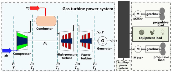
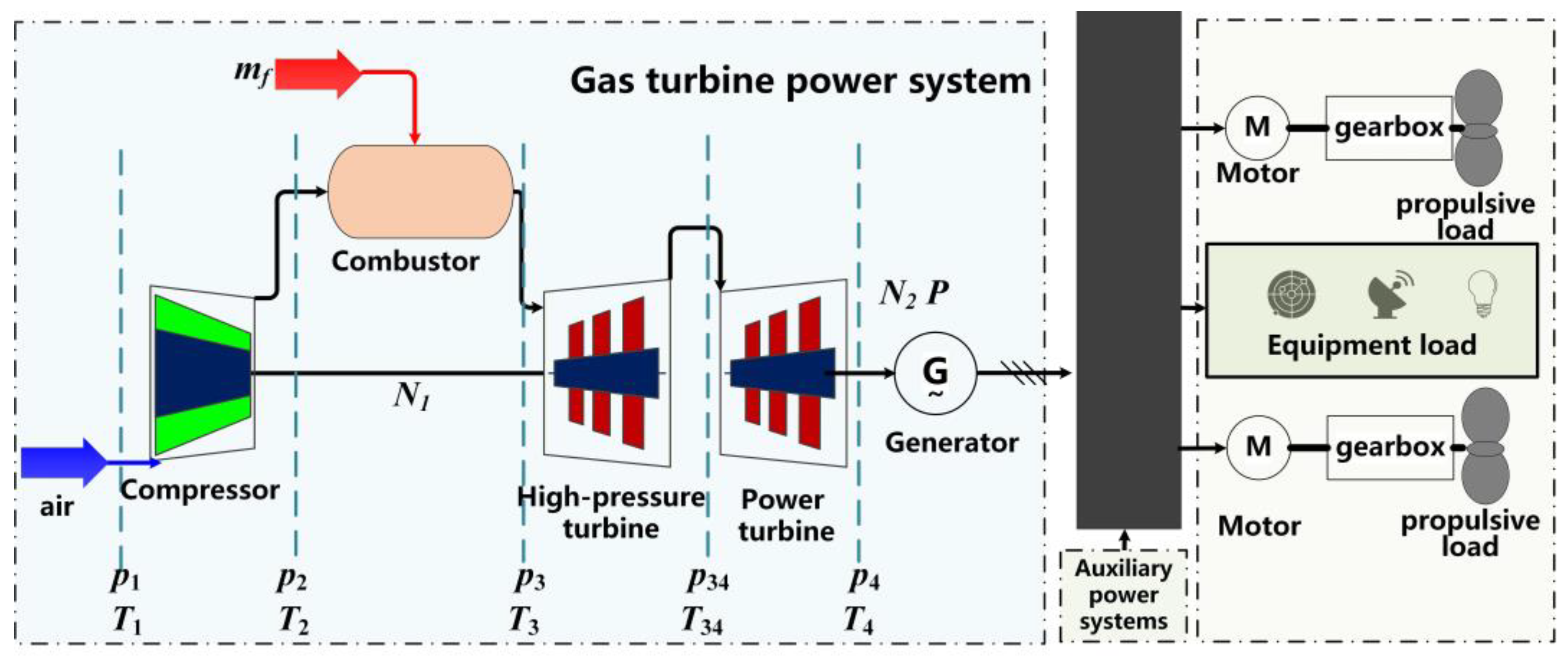
An LM2500+ dual-shaft gas turbine serves as the primary power device for the marine electric propulsion system. The LM2500+ marine gas turbine is a high-performance aero-derivative engine developed by General Electric. As illustrated in Figure 1, the gas turbine consists of a compressor and two turbines. The high-pressure turbine drives the compressor in the gas generator, and the power turbine drives the generator and produces electricity for the marine grid. The output power under full-load design conditions is 31.21 MW and thermal efficiency is 37.75%. The main performance parameters under design conditions are summarized in Table 1.
Figure 1.
LM2500+ gas turbine plant for marine electric propulsion system.
Table 1.
Main performance of LM2500+ gas turbine under full-load design conditions [33].
The gas path sensors are deployed to ensure the comprehensive monitoring of the thermodynamic states. As shown in Figure 1, the measurement variables are summarized in Table 2. The sensors include diaphragm-strain gauge pressure transducers for pressure (p1, p2 and p34), thermocouples for temperature (T1, T2, and T34), magnetic speed pickups for rotational speed (N1 and N2), Coriolis mass flow meter for mass flow rate (mf), and linear variable differential transformer for actuator position (IGV).
Table 2.
Gas path measurements of LM2500+ gas turbine.
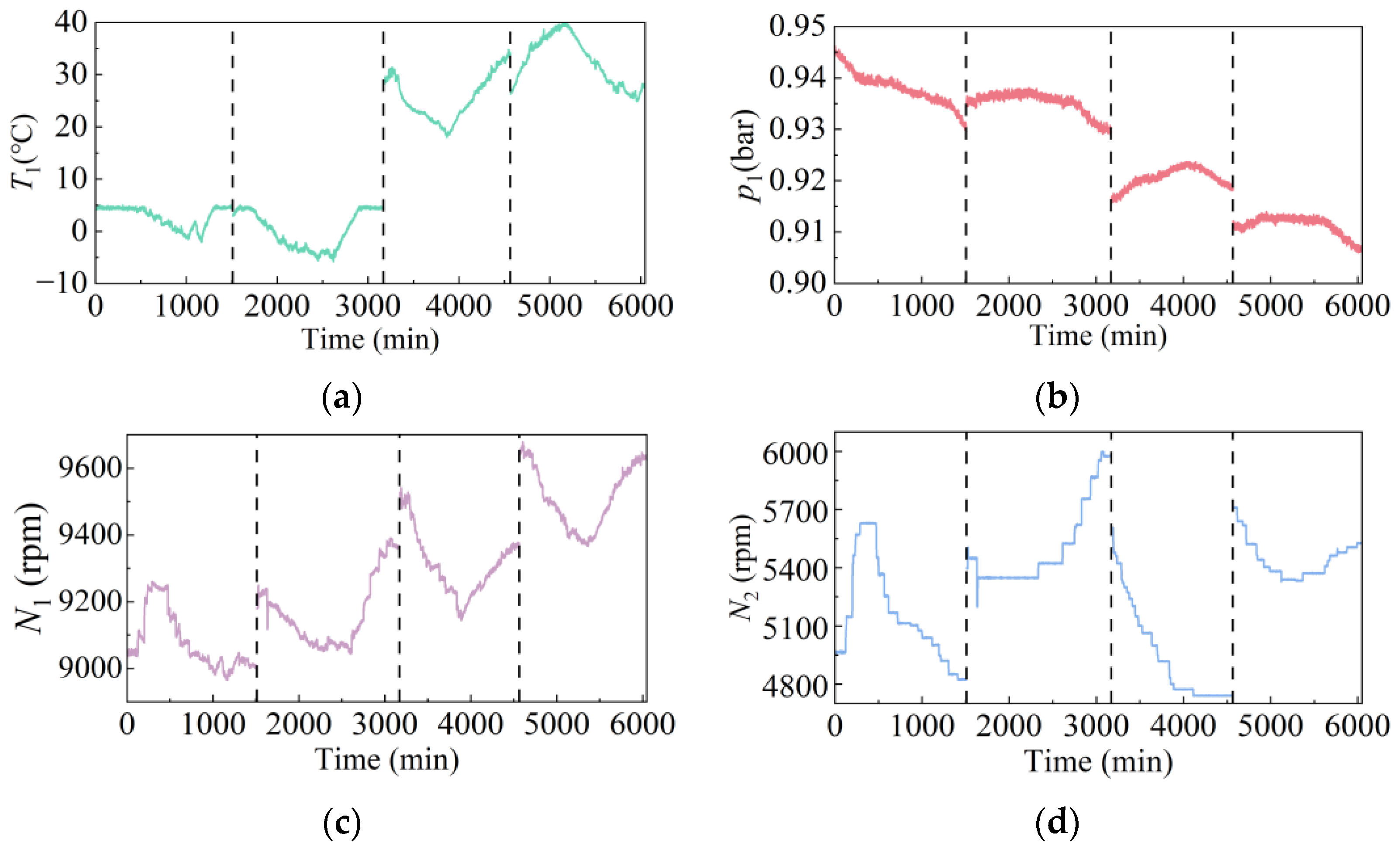
The dataset from the operation data of the LM2500+ gas turbine spans 6044 min. As illustrated in Figure 2, the operation data is divided into four sampling regions (demarcated by vertical dashed lines) to represent different operation conditions. The inlet temperature (T1) ranges from approximately −6 °C to 40 °C. Specifically, regions 1 and 2 capture the gas turbine performance under low-temperature conditions (−6 °C–5 °C), whereas regions 3 and 4 represent high-temperature conditions. The gas generator rotational speed (N1) ranges between 8960 rpm and 9700 rpm, and power turbine rotation speed (N2) ranges between 4700 rpm and 6000 rpm.
Figure 2.
Operation parameters collected from the gas turbine: (a) compressor inlet temperature; (b) compressor inlet pressure; (c) gas generator rotational speed; (d) power turbine rotational speed.
In the total samples spanning 6044 min, the samples in regions 1 and 3 (total 2906 min) are selected for model development, which are further divided into training and validation datasets with an 80%/20% chronological split. The remaining samples are selected as the test dataset for subsequent comparative analysis. Furthermore, three strategies are adopted to prevent information leaks for the time-series prediction. (1) A strict chronological splitting approach is employed rather than random sampling in time-series data to divide the training/validation/test datasets. (2) The data preprocess is implemented after data splitting to prevent statistical information from the validation and test sets from leaking into the training process. (3) The data at the splitting points is processed by purging and embargoing. Purging involves removing any training samples that overlap with the start of the test set. Embargoing involves dropping an initial portion (equal to the input window size) of the test data to further enhance leakage prevention.
2.2. Performance Estimation Based on Mechanism Model
Regarding the LM2500+ gas turbine in this work, the output power sensor is not installed on the gas path instrumentation and measurement system due to the lightweight and space requirements of aero-derivative gas turbines. A mechanism simulation model of a dual-shaft gas turbine is developed to estimate the unmeasured parameters (compressor air flow rate, compressor efficiency, system output power, etc.) based on the measurement data. The mechanism model is established based on the energy and mass balance equations of the Brayton cycle. The detailed modeling process can be seen in previous work [34]. The compressor air flow rate and system output power are generated by the mechanism model, as expressed in the following equations.
where ma is the compressor air flow rate. P is the gas turbine output power. fmech is a steady-state mechanism model of a dual-shaft gas turbine.
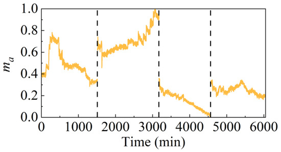
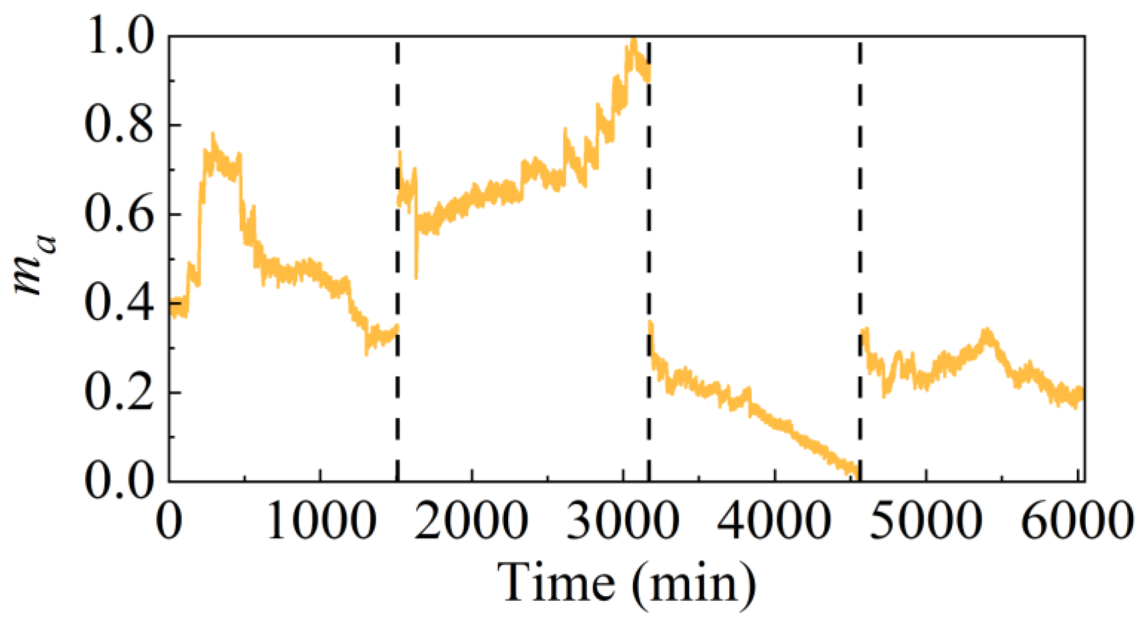
The outputs of the mechanism model serve as the true value for the training and test of our data-driven models. Specifically, Figure 3 shows the normalized compressor air flow rate that corresponds to the input conditions presented in Figure 1. The calculated compressor air flow rate dataset serves as the training resource, which allows the condition-adaptive regulator to acquire prior knowledge of compressor characteristics.
Figure 3.
The calculated compressor air flow rate from the mechanism model.
3. Methodology
3.1. Framework of the Proposed Method
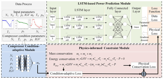
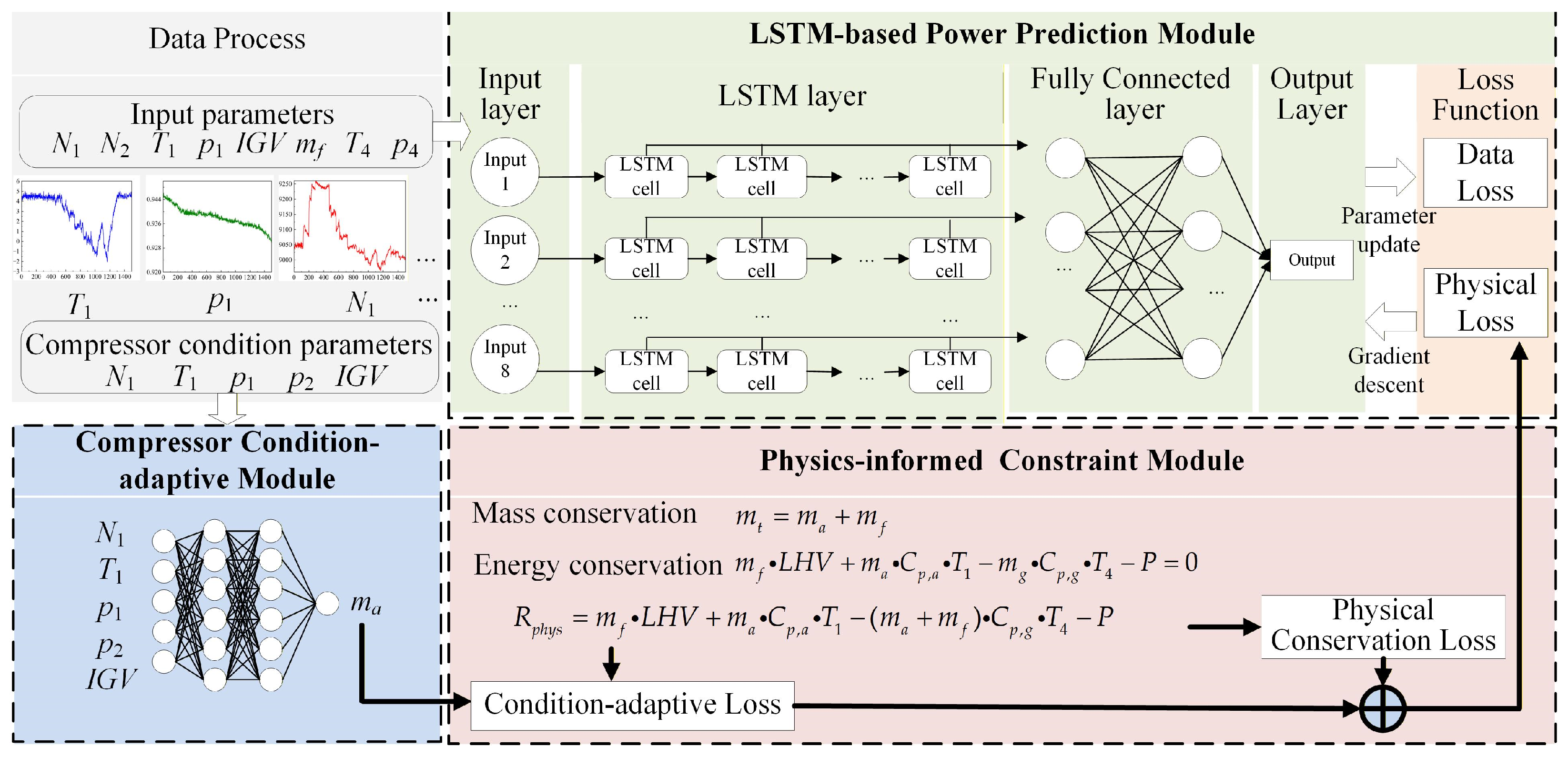
The framework of the proposed CAPI-LSTM method is illustrated in Figure 4. The CAPI-LSTM method embeds the energy balance equation to ensure physical consistency. Furthermore, the compressor air flow rate within the physics-informed loss function is dynamically updated by a compressor condition-adaptive regulator, which is pre-trained to represent the prior knowledge of compressor characteristics. It is noted that the CAPI-LSTM model in this work is mainly applied for short-term power prediction for the purpose of flexible scheduling and the stability of the shipboard microgrid. When the power prediction model occurs, a certain level error due to the fault-causing performance degradation, the CAPI-LSTM model can be periodically retrained offline using recent operation data that reflects the current degradation state.
Figure 4.
Framework of the proposed CAPI-LSTM model.
The three modules of the CAPI-LSTM method are as follows.
(1) LSTM-based power prediction module. This module handles the foundational predictive tasks of the gas turbine. An LSTM network is utilized to predict the marine gas turbine output power according to the sequences of eight boundary parameters.
(2) Physics-informed constraint module. To ensure the physics consistency of the outputs, a physics-informed loss function is incorporated based on the energy balance equation of the gas turbine. In addition to the mean square error (MSE) between the LSTM outputs and training data, the physical residuals of the power predictions are calculated to penalize the outputs that violate the thermodynamic principles.
(3) Compressor condition-adaptive module. A pre-trained MLP network serves as a condition-adaptive regulator that represents the prior knowledge of compressor characteristics. The compressor air flow rate (ma) is identified according to the compressor operation conditions (N1, T1, IGV, p1, and p2). This module enables the physics-informed loss function to adapt to the varying operation conditions.
3.2. Development of the LSTM Power Prediction Model
The LSTM model captures the temporal dependencies from the marine gas turbine operation data through regulated memory retention. The inputs of the LSTM power prediction model include N1, N2, p1, T1, IGV, mf, p4, and T4. At timestep t, the hidden state ht is updated through three types of gates. Mathematically, the update process of an LSTM cell at time step t is formulated as follows.
Forget gate ft:
where is the input matrix. L is the input window length. Wf and bf are the learned weight matrix and bias vector of the forget gate. ht−1 is the previous hidden state. is the sigmoid activation function.
Input gate it:
where Wi and bi are the learned weight matrix and bias vector of the input gate. is the candidate cell state. is the hyperbolic tangent activation function.
The cell state ct is updated as follows.
where is the element-wise multiplication Output gate ot:
where Wo and bo are the learned weight matrix and bias vector of the output gate.
The hidden state ht is calculated as follows.
Finally, the extracted temporal features are subsequently mapped to the power output through a fully connected layer.
where is the predicted output power. H is the output window length. WFC and bFC are the learned weight matrix and bias vector of the fully connected layer.
3.3. Formation of the Physics-Informed Loss Function
The CAPI-LSTM model incorporates the thermodynamic equation into the loss function to realize the robust power prediction across the full operation envelope of a marine gas turbine plant. The physics-informed loss function of the LSTM model is derived from the mass and energy balance equations. The energy balance equation for the marine gas turbine is expressed as follows. The input energy terms of the gas turbine consist of fuel heat and compressor inlet air enthalpy, and the output energy terms consist of turbine exhaust enthalpy and output power.
where LHV denotes the fuel lower heating value. and are the specific heat capacity of air and exhaust gas, which are the function of gas temperature. ma and mg are the mass flow rates of the compressor and the turbine.
The units of the variables in the energy balance equation are as follows: mass flow rates (ma and mf) in kg/s, LHV in MJ/kg, the specific heat capacities ( and ) in MJ/(kg∙K), temperatures (T1 and T4) in K, and power (P) in MW = MJ/s. All terms in the energy balance equation are dimensionally consistent with the power unit of MW.
According to the mass balance equation, the relation between ma and mg can be expressed as follows.
By substituting Equation (9) into the energy balance Equation (8), the unified physical residual Rphys can be obtained.
In Equation (10), the LHV is set to a constant value of 48 MJ/kg. and are modeled as the functions of gas temperature. mf, T1, and T4 are the inputs from gas path sensors. ma is the learned compressor air mass flow rate from the CAPI-LSTM model. P is the predicted output of the CAPI-LSTM model.
The corresponding physical conservation loss Lcons is defined as follows.
During the training process, the physics parameters ma and LHV in Equation (10) are inferred by the PINN algorithm. However, a critical feature of the CAPI-LSTM model is that the compressor air flow rate ma is a condition-related variable. In this work, the condition-adaptive loss Ladapt is introduced to ensure that the learned compressor air flow rate in the physics-informed loss function keeps consistency with the condition-adaptive regulator.
where is the reference compressor mass flow rate from the condition-adaptive regulator. is the learned compressor air mass flow rate.
Finally, the physics-informed loss function Lphys is the sum of physical conservation loss Lcons and the condition-adaptive loss Ladapt, which is expressed as follows.
The total loss function Ltotal of training the CAPI-LSTM model during the training process is a weighted combination of the data-driven loss Ldata and the physical informed loss Lphys.
where Ldata represents the MSE between the predictive power and true value. is a regularization parameter, which is introduced to balance the trade-off between empirical data fitting accuracy and the penalty for deviating from the underlying thermodynamic laws. A larger strengthens the contribution of the physical constraints, thereby enhancing the physical consistency of the energy and mass balance. Conversely, a smaller prioritizes fitting the training data more closely. The determination of the optimal value is discussed in Section 4.1.1.
3.4. Compressor Condition-Adaptive Regulator of Physics-Informed Loss Function
In marine gas turbine systems, the compressor air mass flow rate (ma) is a complex function of corrected speed, pressure ratio, and IGV opening. The compressor operation state varies significantly under different load operations. As indicated in Equation (10), the accuracy of ma is highly critical to maintaining the validity of the embedded physics-informed loss function. In this work, the condition-adaptive regulator is specifically designed to ensure the thermodynamic consistency of the physics-informed loss function across the full operation envelope. Physically, the condition-adaptive regulator serves as a neural network-based model to identify the air flow rate from the compressor characteristic map. This regulator prevents the physics loss function from significant errors even when the gas turbine deviates from its design conditions.
The condition-adaptive regulator for estimating the compressor air flow rate is a pre-trained MLP network. The MLP model consists of two hidden layers with 64 neurons, using ReLU activation functions after each hidden layer.
According to the compressor characteristics, the compressor reduced flow rate is the function of rotational speed and pressure ratio, which is expressed as follows.
As shown in Equation (16), the compressor air flow rate relates to the parameters of N1, T1, p1, p2, and IGV. Therefore, the input of the MLP model for the condition-adaptive regulator is defined as Xcomp = [N1, T1, p1, p2, IGV].
To ensure the reliability of the condition-adaptive module, the MLP model is pre-trained using a supervised learning scheme before integration into the CAPI-LSTM framework. The ground truth labels for the air mass flow rate are generated via the mechanism-based simulation model described in Section 2.2. The network weights are optimized to minimize the error between the MLP predictions and mechanism-derived ma. The model achieves an RMSE of 0.735, with the maximum relative error across the entire test set strictly limited to 0.86%.
4. Results and Discussion
4.1. Effect of the Physics Loss and Condition-Adaptive Modules
4.1.1. Predictive Performance Comparison of Ablation Study
To evaluate the contribution of each core component within the CAPI-LSTM method, an ablation study was conducted. The predictive performance of the CAPI-LSTM model was compared with two derivative models. The three compared models for ablation study are summarized as follows.
- CAPI-LSTM: The complete framework proposed in this study with both physics-informed loss function and condition-adaptive module.
- Standard physics-informed LSTM (standard PI-LSTM): The physics-informed loss function is retained, while the condition-adaptive module is removed. The standard PI-LSTM model ignores the condition-adaptive nature of the compressor air flow rate.
- Pure LSTM: The physics-informed loss and condition-adaptive regulator are both removed to evaluate the baseline LSTM performance.
The models were implemented using the PyTorch 1.10.2 deep learning framework. To ensure fair comparisons, all models were conducted on the same hardware environment. The hardware specifications include an AMD Ryzen 5 4600H CPU (3.00 GHz) and an NVIDIA RTX 3060 GPU.
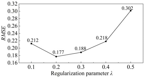
The Adam optimizer was employed for model training. The initial learning rate was set to 0.001. The batch size was set to 32 to balance training stability and memory efficiency. Training was conducted for 100 epochs. The LSTM model comprises a single LSTM layer with 64 hidden units followed by two fully connected layers with 64 and 32 neurons, respectively. To ensure a balanced optimization, the regularization parameter was tuned via a grid search in the interval [0.1, 0.5]. Figure 5 illustrates the impact of different values on the model’s prediction performance on the validation set. The final model adopts 0.2 with the lowest RMSE of 0.177.
Figure 5.
Sensitivity analysis of the regularization parameter
The root mean square error (RMSE), maximum absolute error (MaxAE), and coefficient of determination (R2) of the three models are summarized in Table 3.
Table 3.
The predictive performance comparison of the ablation study.
The purely LSTM model exhibits an RMSE of 0.493, an R2 of 0.970, and a MaxAE of 1.041. The standard PI-LSTM model reduces the RMSE to 0.291 and increases the R2 to 0.989. It means that the incorporation of the energy balance constraints into the loss function is sufficiently meaningful to enhance the overall prediction performance of marine gas turbine output power. However, the MaxAE of the PI-LSTM model increases to 1.130 MW, which means that the constant air flow rate within the physics-informed loss function may cause a significant peak error when the gas turbine operates far away from design conditions. The proposed CAPI-LSTM model overcomes this limitation by introducing the condition-adaptive regulator to adjust the compressor air flow rate under varying operation conditions. The CAPI-LSTM model achieves the lowest RMSE of 0.177 and MaxAE of 0.729. Furthermore, the R2 of 0.996 is highest. The results show that the CAPI-LSTM model is most suitable for power prediction across the entire operation envelope.
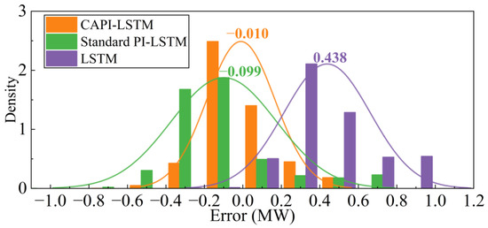
The error histogram and probability density function (PDF) plots of three comparison models are shown in Figure 6. The pure LSTM model suffers from the widest error distribution with the highest mean error of 0.438 MW. The standard PI-LSTM model shows a broader PDF curve with a peak density of −0.099 MW. The results confirm that the incorporation of the energy balance equation into the physics-informed loss function can effectively enhance the prediction performance. The proposed CAPI-LSTM model maintains superior stability and minimal error for predicting the marine gas turbine output power. The CAPI-LSTM model exhibits the most concentrated distribution, and its peak density occurs at the value closest to zero (−0.010 MW). The comparison results indicate that the condition-adaptive regulator for the energy balance equation is critical to achieve high-accuracy power prediction across the full operation envelope.
Figure 6.
Error histogram and probability density function of the ablation study.
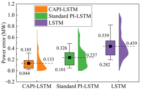
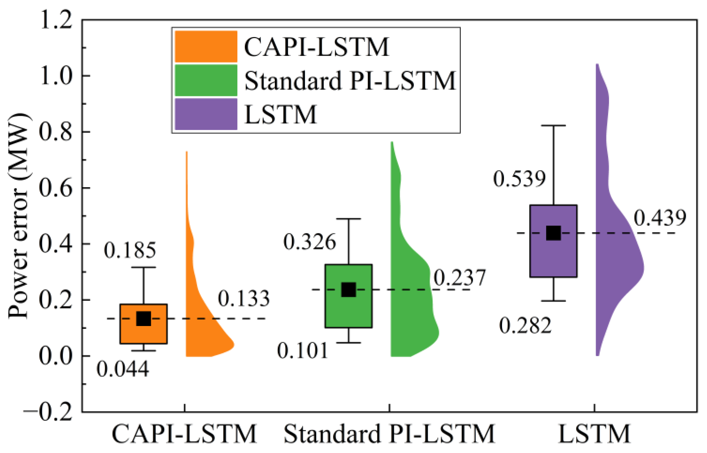
Furthermore, the violin plot of the absolute error distribution is shown in Figure 7. The pure LSTM model shows the poorest predictive performance with the highest average absolute error (0.439 MW) and its violin tail is much heavier, with an interquartile range of [0.282, 0.539]. By embedding the physics-informed loss function, the average absolute error of the PI-LSTM model is decreased to 0.237 MW and the interquartile range is narrowed to [0.101, 0.326]. The proposed CAPI-LSTM model exhibits the best prediction performance with the lowest average absolute error (0.133 MW) and the narrowest interquartile range ([0.044, 0.185]). Its violin shape shows a more concentrated error distribution near zero. The results show that the incorporation of the physics loss function with a compressor condition-adaptive regulator can effectively enhance the prediction accuracy of marine gas turbine output power under different operation conditions.
Figure 7.
Violin plot of absolute prediction errors of the ablation study.
To further evaluate the statistical significance of model performance differences, a paired t-test is carried out on the absolute prediction errors of the different models. The paired t-test results of the ablation study are summarized in Table 4. The mean values of the error difference are more than zero. The t-statistics for the comparisons of PI-LSTM (44.154) and LSTM (80.912) are exceptionally high, and all p-values are almost zero (significantly lower than the threshold level of 0.05). These results prove that the performance improvement of the proposed CAPI-LSTM model is statistically significant and not due to random variation.
Table 4.
Paired t-test results of the ablation study.
4.1.2. Physical Consistency Analysis of the CAPI-LSTM Model
During the training process of the CAPI-LSTM model, the learned physical parameters of compressor air flow rate (ma) and fuel lower heat value (LHV) directly determine the reliability of the physics loss function. Unlike the standard PI-LSTM model with a constant ma, the CAPI-LSTM model recognizes ma as a varying parameter that is determined by the compressor operation conditions. As a result, the CAPI-LSTM model employs a condition-adaptive loss function Ladapt to ensure that the learned ma values follow the outputs of the pre-trained MLP model.
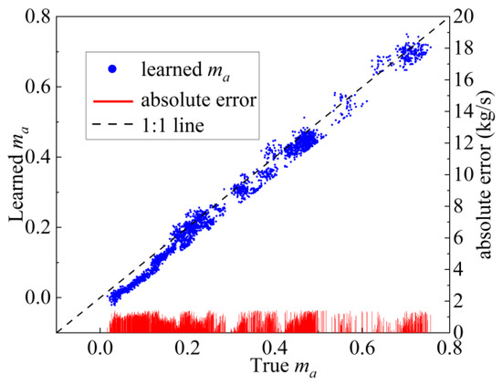
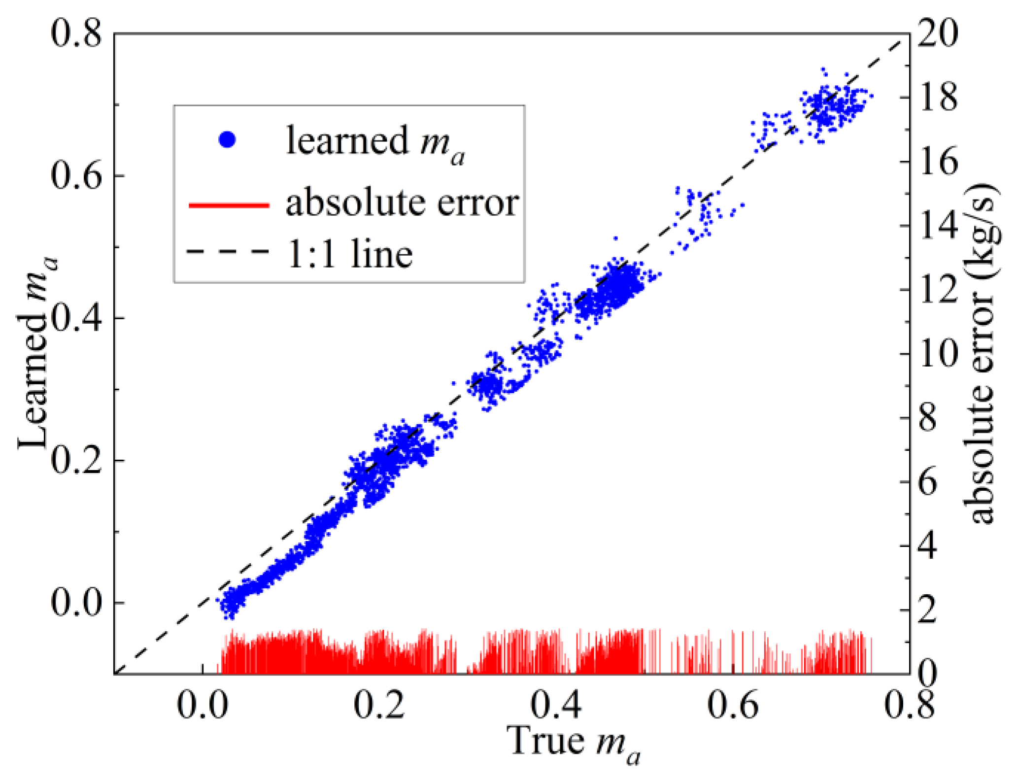
The error of the learned ma during the CAPI-LSTM training process is shown in Figure 8. The learned ma values under different operation conditions are highly consistent with the true value from the mechanism model. The maximum absolute error is less than 1.43 kg/s. The results indicate that the learned physical parameters of the CAPI-LSTM model can effectively capture the complex compressor flow characteristics under varying operation conditions, which verifies the physical consistency for the full operation conditions of marine gas turbines.
Figure 8.
Error of the learned ma values for the physical consistency analysis. Blue dot is the learned ma, the red line is the absolute error, and the dash black line is the 1:1 line.
4.1.3. Analysis of Generalization to Unseen Operation Conditions
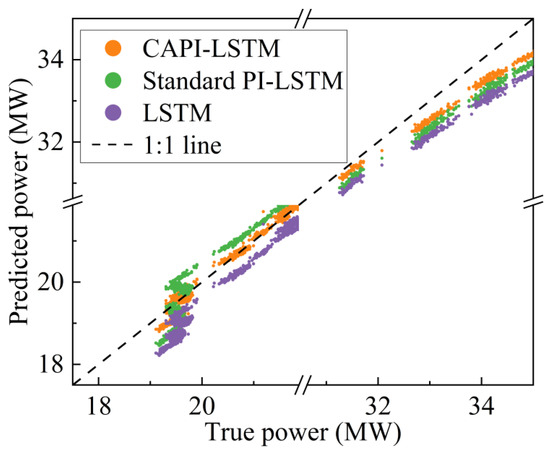
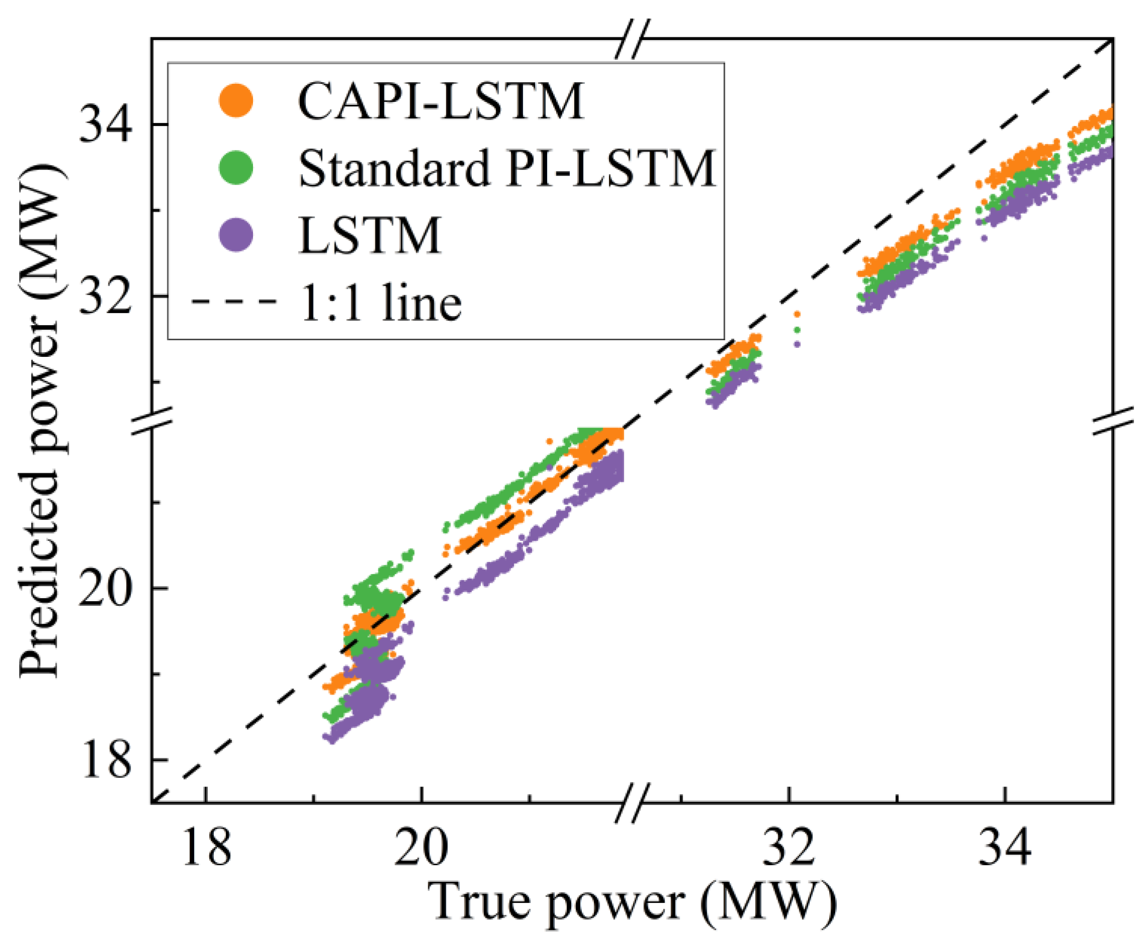
To further evaluate the robustness and generalization capability of the CAPI-LSTM model, the prediction performance is specifically analyzed under two unseen operation conditions which are beyond the power range of the training data (30–35 MW). The prediction performances under the conditions of the low-power range (19–22 MW) and high-power range (30–35 MW) are illustrated in Figure 9. The pure LSTM model demonstrates the poorest prediction performance. It consistently underestimates the output power under the unseen load conditions and exhibits high variance in the low-load region. The standard PI-LSTM model achieves moderate predictive performance with visible deviations in the high-power region. It is mainly because the constant physical parameter fails to match the actual compressor air flow behavior under unseen conditions. The CAPI-LSTM model exhibits the highest alignment with the true value (dash line) across both the low- and high-power ranges.
Figure 9.
Predictive performances under unseen operation conditions. The dash black line is the 1:1 line.
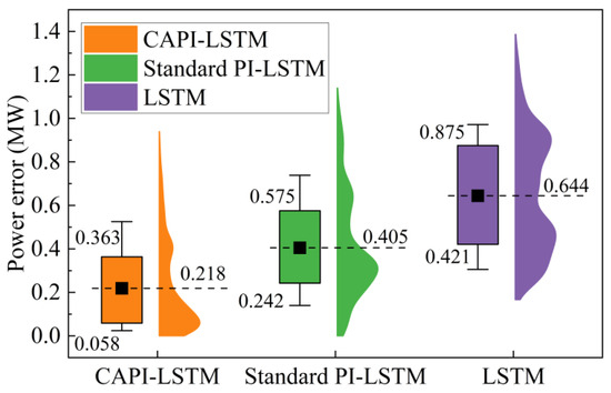
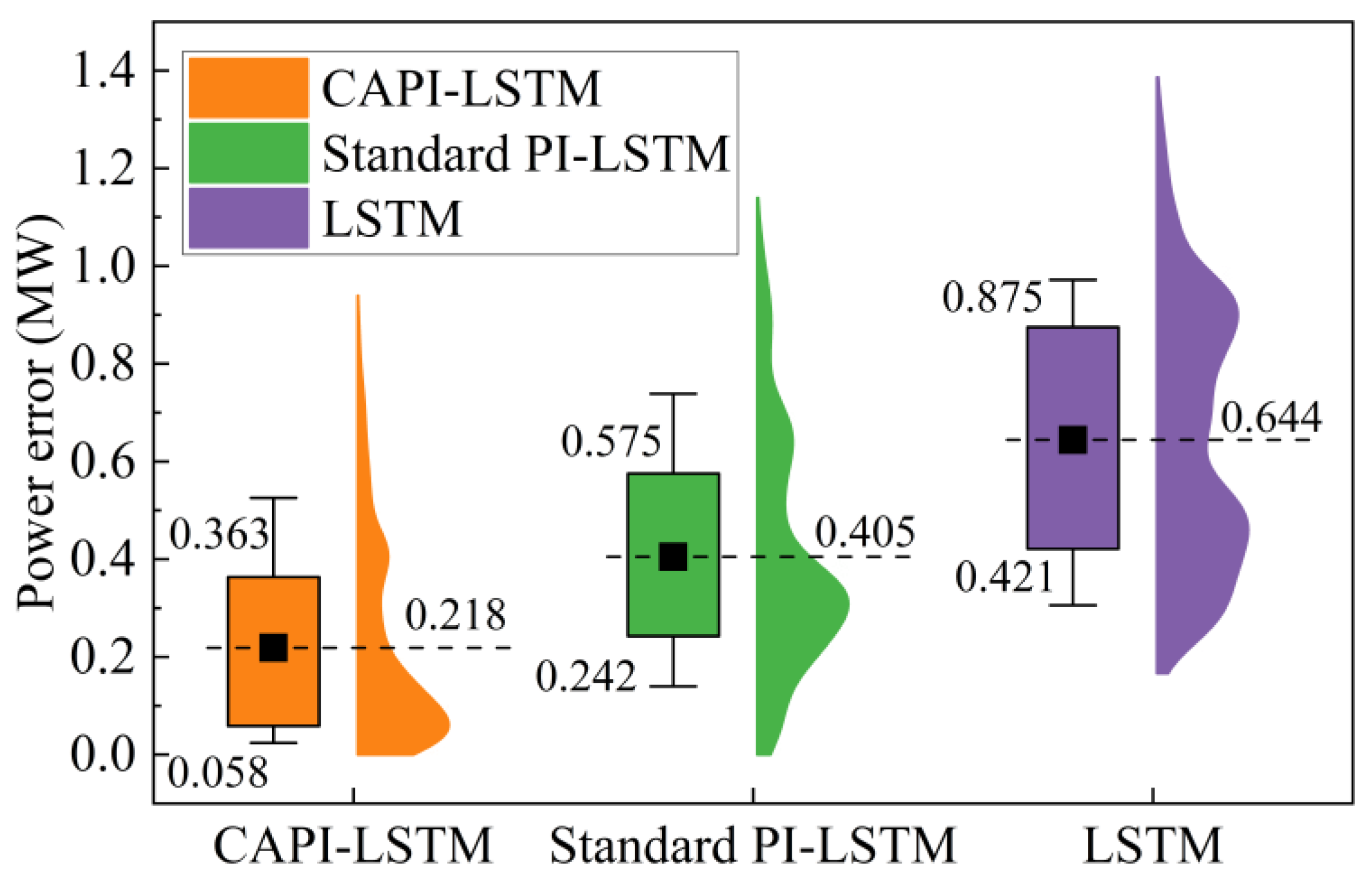
The absolute error distributions under the unseen operation conditions are shown in Figure 10. The pure LSTM model shows the poorest generalization capability. It achieves the highest average absolute error (0.644 MW) and the widest interquartile range of [0.421, 0.875]. This performance indicates that the pure LSTM model lacks reliable extrapolation when facing unseen training conditions. The standard PI-LSTM model partly improves predictive stability by embedding the physical constraints into the training loss function. It achieves a lower average error of 0.405 MW and a relatively narrow interquartile range of [0.242, 0.575]. The proposed CAPI-LSTM model exhibits the best generalization capability. Its violin shape is the most concentrated near zero with an average of only 0.218 MW and the narrowest interquartile range of [0.058, 0.363]. This superior generalization is mainly due to the condition-adaptive regulator, which can effectively ensure the air flow rate (ma) in the physics-informed loss function remains valid across the full operation envelope.
Figure 10.
Absolute error distributions under the unseen operation conditions.
4.2. Comparative Analysis with the State-of-the-Art Data-Driven Model
To further validate the performance of the proposed CAPI-LSTM model, a comparative analysis is conducted against three state-of-the-art (SOTA) data-driven models, which include MLP [34], Transformer [35], and CNN-LSTM [36]. The MLP model consists of three fully connected layers with 9, 64, 64, and 1 neuron, respectively. The ReLU activation function is applied after each hidden layer. The Transformer model employs a multi-head self-attention mechanism with 8 attention heads, 3 encoder layers, and a model dimension of 64. The feedforward network within each encoder layer has a dimension of 512. The CNN-LSTM model combines convolutional and recurrent architectures for temporal feature extraction. The CNN component consists of three convolutional layers with 64, 128, and 128 output channels, respectively. Each convolutional layer uses a kernel size of 3. The LSTM component employs single layer with 64 hidden units per layer.
The RMSE, MaxAE, and R2 are summarized in Table 5. The MLP model exhibits the poorest performance with the highest RMSE of 0.652 and the lowest R2 of 0.947. The result indicates that a simple feedforward structure cannot effectively capture the complex temporal dependencies and nonlinear thermodynamics in a marine gas turbine. The Transformer and CNN-LSTM models achieve improved RMSE and R2 values, while their MaxAE values are relatively high. The Transformer produces the highest MaxAE of 1.750 MW. It means that the pure data-driven models struggle to handle the high-variation conditions in marine power systems. The proposed CAPI-LSTM model outperforms all compared SOTA models. It achieves the lowest RMSE of 0.177 MW and the highest R2 of 0.996. Compared with the CNN-LSTM, which is the strongest purely data-driven candidate, the CAPI-LSTM model reduces the RMSE by 58.5% and reduces the MaxAE by 38.6%. These results demonstrate that the proposed CAPI-LSTM model is more effective to capture the true performance of the marine gas turbine output power.
Table 5.
The prediction results of the compared models.
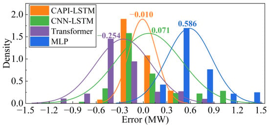
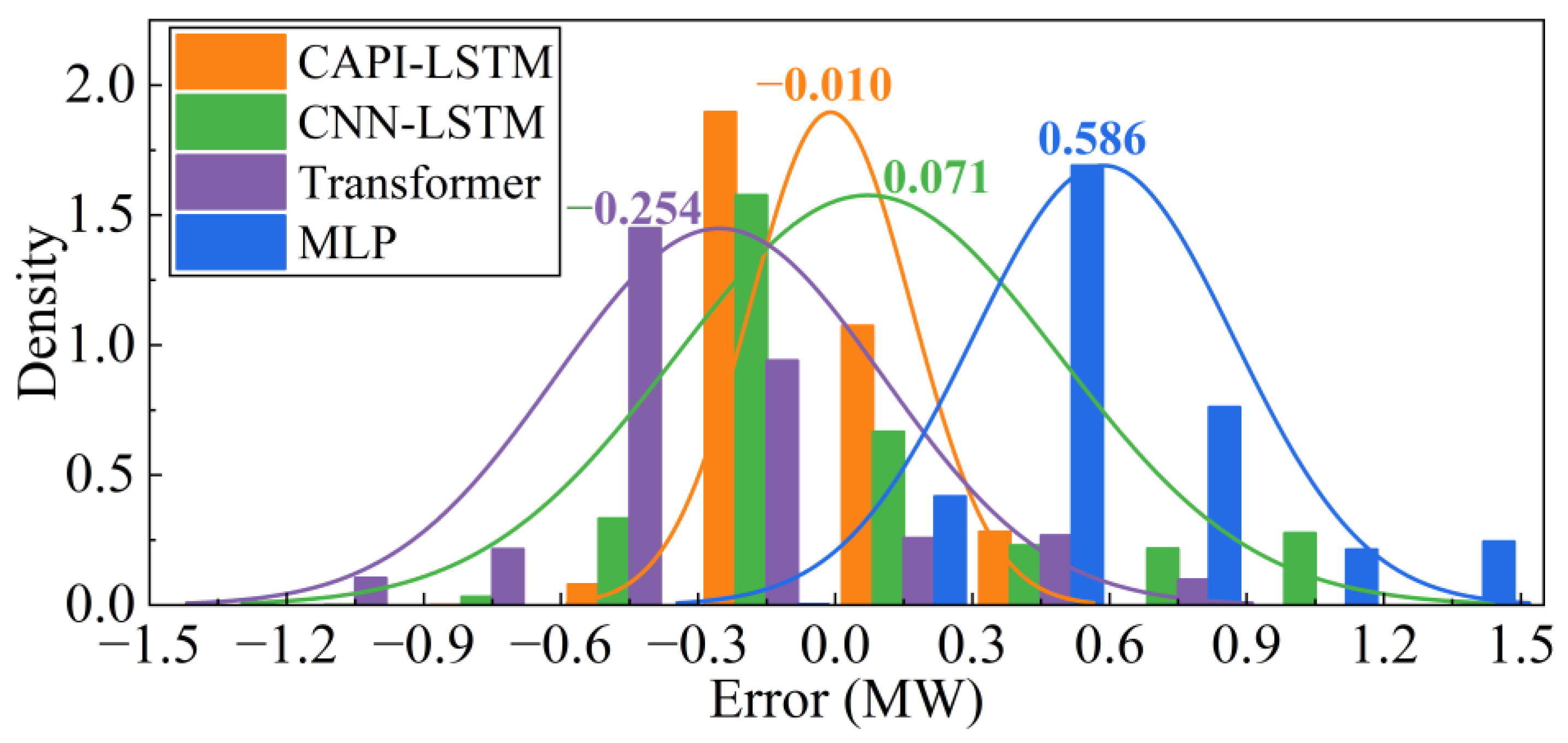
The error histogram and PDF plots of the SOTA models are illustrated in Figure 11. The CAPI-LSTM model shows a highly concentrated PDF curve with a peak density of −0.010 MW. In contrast, the MLP model exhibits the highest bias with a peak density of 0.586 MW. The peak density point of the Transformer model is −0.254 MW. The CNN-LSTM model is more centered, with a peak density of 0.071 MW, while its distribution is much wider than the CAPI-LSTM model.
Figure 11.
Error histogram and probability density function of SOTA models.
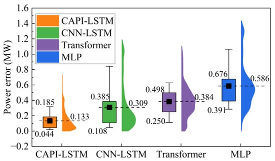
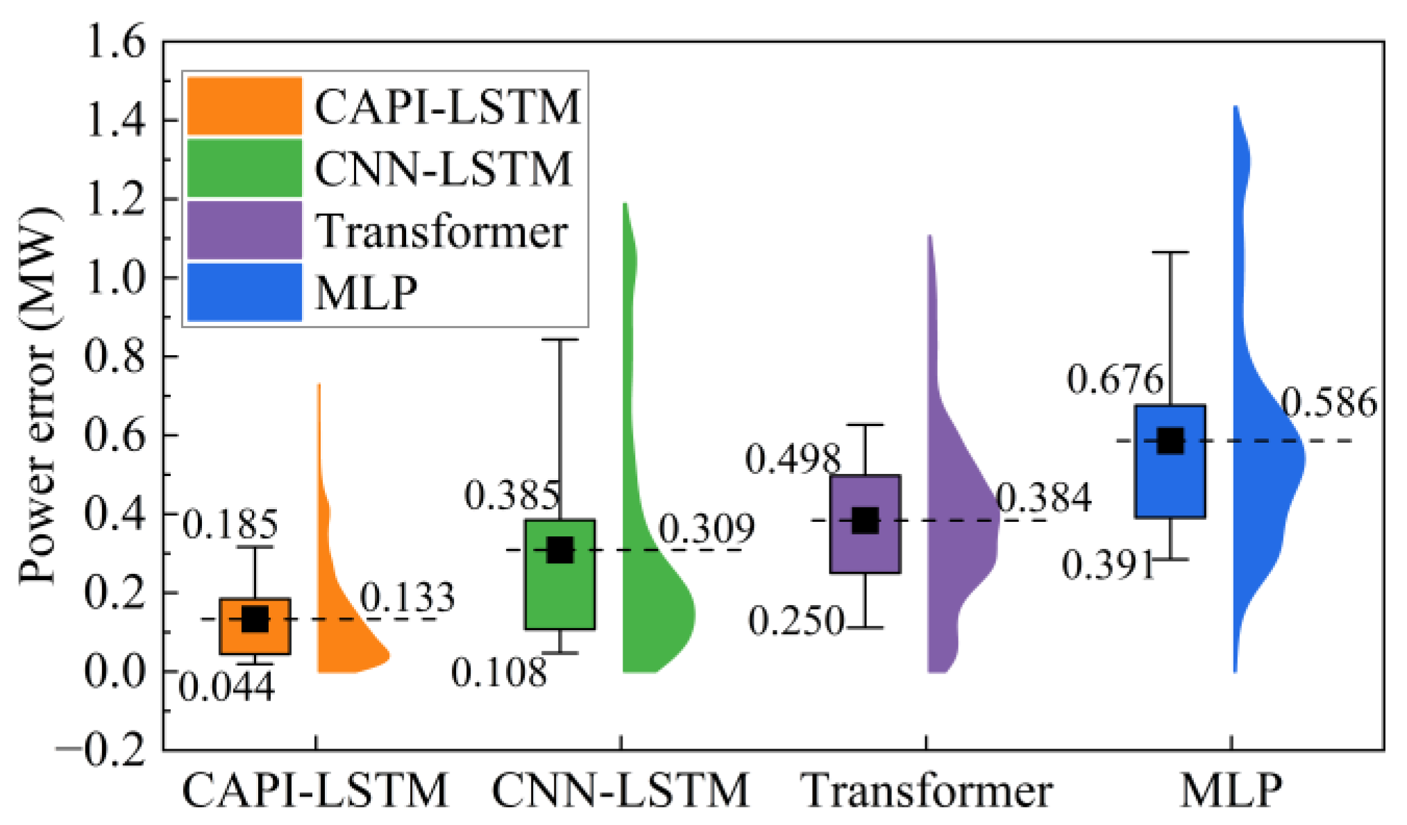
The magnitude and stability of the prediction errors were further quantified using violin plots, as illustrated in Figure 12. The MLP and Transformer models display significant dispersion. Their average errors reach 0.586 MW and 0.384 MW, respectively. The extended tails in their violin plots are more than 0.8 MW. It reflects a high frequency of large outliers during the prediction process. The CNN-LSTM model offers improved robustness, with an average error of 0.309 MW. However, its interquartile range is relatively wide. The CAPI-LSTM model demonstrates superior precision than the three SOTA models. It achieves the lowest average error of 0.133 MW, with a reduction of approximately 56.9% compared to the CNN-LSTM model. The narrowest interquartile range ([0.044, 0.185]) further proves the effectiveness of the CAPI-LSTM model across the full operation envelope.
Figure 12.
Violin plot of absolute prediction errors of the SOTA models.
The paired t-test results comparing the CAPI-LSTM model with the SOTA models are summarized in Table 6. The mean values of error difference in all evaluated pairs are positive, and the t-statistics are remarkably high. Specifically, the mean value and t-statistic for the comparisons of MLP reach 0.453 and 95.153. Moreover, all p-values are significantly lower than 0.001. These statistical metrics confirm that the proposed CAPI-LSTM model is more statistically significant than the purely data-driven SOTA models.
Table 6.
Paired t-test results of the SOTA models.
In summary, the comparative analysis reveals that the proposed CAPI-LSTM model significantly outperforms the purely SOTA data-driven models. Although the advanced architectures, such as Transformer and CNN-LSTM, can capture complex temporal features from the training dataset, they still suffer from systematic bias and instability due to the lack of domain knowledge guidance. The CAPI-LSTM model effectively enables reliable and robust power prediction across the full operation envelope. This is because the condition-adaptive regulator provides dynamic physical guidance of the embedded physics-informed loss function.
4.3. Computational Efficiency Analysis
To evaluate the computational efficiency, all models are tested on a workstation equipped with Intel(R) Core (TM) i9-10900K CPU (@ 3.70 GHz), 32.0 GB of RAM (2667 MHz), and an NVIDIA GeForce RTX 3080 GPU (10 GB). The models are executed in a Python 3.6.0 environment and a 64-bit Windows operating system.
The computational times of all models are summarized in Table 7. The results demonstrate that all machine learning models are dramatically faster than the mechanism model. The mechanism model requires approximately 9028 s to process the entire test dataset. This is mainly due to the iterative calculation of solving thermodynamic equations. In contrast, the machine learning models complete the same prediction task in approximately 2 s.
Table 7.
Comparison of computational times.
Although the proposed CAPI-LSTM model integrates a physics-informed loss function and a condition-adaptive regulator, its total training time (2.63 min) remains competitive, where the training of the condition-adaptive regulator only accounts for 0.56 min. The simpler networks such as LSTM (1.71 min) and MLP (1.65 min) demonstrate faster training speed, while their prediction accuracy is substantially lower. The other complex networks such as CNN-LSTM (2.74 min) and Transformer (2.81 min) require longer training time. Most importantly, the prediction time of the CAPI-LSTM model is only 2.08 s, which is almost identical to the other machine learning models. The results indicate that the proposed CAPI-LSTM model achieves competitive computational efficiency compared to the other machine learning models while providing a superior power prediction accuracy for marine gas turbine plants.
4.4. Effect of the Measurement Noise
The performance of the proposed method is also tested in the presence of measurement noise. Based on the comparison results in Section 4.1 and Section 4.2, the standard PI-LSTM and CNN-LSTM models are identified as the two most competitive baseline models. Therefore, they are selected to provide a benchmark for the noise resilience experiment.
The measurement noise is assumed as a Gaussian distribution with zero average. The standard deviations σ of the measurements in the LM2500+ gas turbine are derived from references [37,38]. Specifically, the standard deviation of pressure sensor is 0.25%, the temperature sensor is 0.4%, the rotational speed sensor is 0.05%, the fuel mass flow rate sensor is 0.4%, and the IGV sensor is 1%.
The predictive performance in a noisy environment is summarized in Table 8. The purely data-driven CNN-LSTM model exhibits the lowest performance. The RMSE increases from 0.427 to 0.664, MaxAE increases from 1.188 to 1.536 MW, and R2 drops from 0.977 to 0.852. The results indicate that a purely data-driven model cannot effectively maintain prediction accuracy in a noisy environment. The standard PI-LSTM model outperforms the CNN-LSTM model due to the incorporated physical loss. However, the constant air flow rate in the physics-informed loss function fails to fully mitigate the effect of measurement noise. In contrast, the CAPI-LSTM model achieves the best performance. Compared with the PI-LSTM model, the RMSE (0.186) and MaxAE (0.763 MW) of the CAPI-LSTM model decrease by approximately 52.2% and 42.8%. This improvement occurs because the condition-adaptive regulator mitigates the effect of measurement noise by dynamically ensuring thermodynamic consistency.
Table 8.
Comparison of predictive performance under noisy conditions.
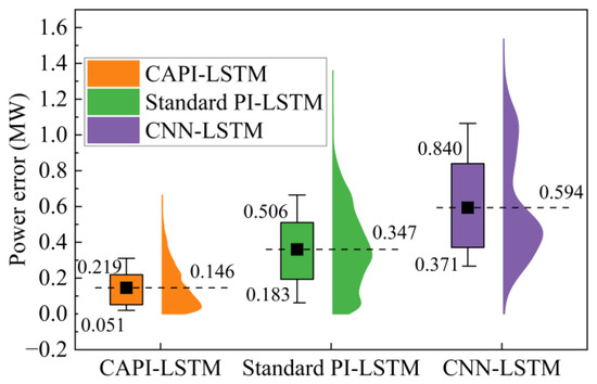
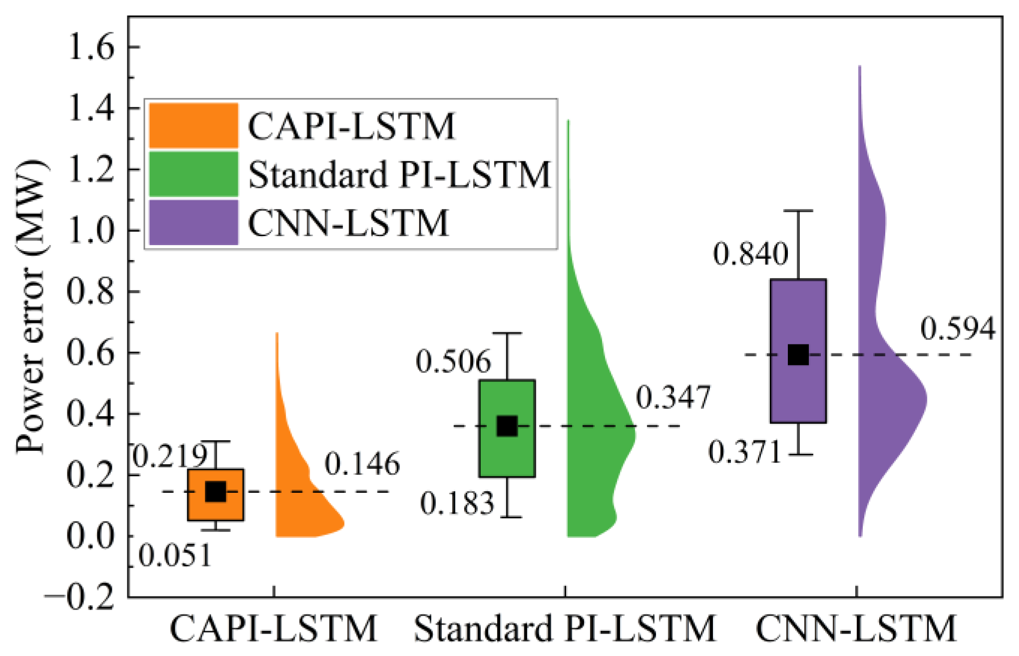
The violin plot of the absolute error distribution in a noisy environment is shown in Figure 13. The CAPI-LSTM model achieves the lowest average error (0.146 MW) and the narrowest interquartile range ([0.051, 0.219]). The standard PI-LSTM and CNN-LSTM models demonstrate much poorer prediction performance in a noisy environment. The average errors of the PI-LSTM (0.347 MW) and CNN-LSTM (0.594 MW) models reach a much higher level, and their violin tails are significantly heavier. The absolute errors exceeding 1.0 MW are frequently observed in the PI-LSTM and CNN-LSTM models. The results confirm that the CAPI-LSTM model achieves the superior capability in noise immunity due to the integration of the physics-informed loss function with a condition-adaptive regulator. Consequently, the CAPI-LSTM model ensures stable and accurate power predictions under measurement uncertainty.
Figure 13.
Violin plot of absolute prediction errors under measurement noise.
4.5. Validation on Other Gas Turbine
The proposed CAPI-LSTM method is applied to an F-class single-shaft heavy-duty gas turbine to validate its generalizability across different gas turbine types. The design output power of this F-class turbine is 310 MW. A dataset of 3360 historical operation samples is collected for model training and testing. The first 1920 samples are allocated for model development, and the remaining samples are used for model testing.
The results of the CAPI-LSTM, standard PI-LSTM, and CNN-LSTM models are summarized in Table 9. Under different gas turbine configurations and power scales, the CAPI-LSTM model still maintains an exceptionally high prediction accuracy. It achieves the highest R2 (0.997), which is almost identical to the result of the LM2500+ gas turbine. The purely data-driven CNN-LSTM model demonstrates the poorest performance with the lowest R2 (0.971). Regarding the error distribution, the interquartile range ([0.511, 1.627]) of the CAPI-LSTM is the narrowest compared with the other evaluated models. These results indicate that the CAPI-LSTM method maintains stable prediction accuracy across different gas turbine types. This is because the embedded physics-informed loss function is derived from the fundamental Brayton cycle. To adapt the model to other gas turbines, the condition-adaptive regulator and CAPI-LSTM model only need to be retrained with the new dataset.
Table 9.
Predictive performance and absolute error distribution on a F-class gas turbine.
5. Conclusions and Future Work
5.1. Conclusions
A CAPI-LSTM framework for marine gas turbine power prediction is proposed to enhance the accuracy and generalization capability across the full operation envelope. The key contribution lies in constructing an MLP-based condition-adaptive model to guide the inference of compressor air flow rate within the embedded thermodynamic equations. This framework enables the dynamic adjustment of the physics-informed loss function in response to varying operation conditions, which can ensure the prediction model outputs maintain rich generalization capacity under unseen operation conditions. The main conclusions are summarized as follows:
(1) The condition-adaptive module plays a critical role in improving power prediction accuracy. The ablation study confirms that the condition-adaptive mechanism significantly enhances model robustness and accuracy. The CAPI-LSTM achieved an RMSE of 0.177 MW, with a reduction of approximately 66.1% compared to the pure LSTM model and 39.2% compared to the standard PI-LSTM. The paired t-test results further prove the statistical significance of the CAPI-LSTM model improvements.
(2) Physical consistency analysis validates that the proposed model accurately captures the complex thermodynamic characteristics under varying operation conditions. The learned compressor air flow rate maintains high consistency with the mechanism model, and the maximum absolute error is less than 1.43 kg/s. This means that the physics-informed loss function effectively guides the model to strictly adhere to physical laws.
(3) The condition-adaptive mechanism ensures generalization capability under unseen operation conditions. Under the unseen low-power (19–22 MW) and high-power (30–35 MW) regions, the CAPI-LSTM model demonstrates superior generalization capabilities, with an average of only 0.218 MW and the narrowest interquartile range of [0.058, 0.363].
(4) The proposed CAPI-LSTM model achieves higher predictive accuracy compared with the SOTA models. The CAPI-LSTM reduces the RMSE by 58.5% and reduces the MaxAE by 38.6% compared with the best-performing CNN-LSTM model.
(5) The proposed CAPI-LSTM model achieves superior performance in noise immunity and transferability to other types of gas turbines. The condition-adaptive mechanism can decrease the RMSE and MaxAE by approximately 52.2% and 42.8% compared with the PI-LSTM model in a measurement noise environment. The CAPI-LSTM model can effectively maintain the considerable level of R2 on different types of gas turbines.
5.2. Future Work
The proposed method does not specifically address the degradation indices caused by gas path faults (such as fouling and corrosion). The CAPI-LSTM model in this work should be periodically retrained offline using recent operation data that reflects the current degradation state. Determining a proper retraining period or developing an online degradation adaptive strategy to maintain high prediction accuracy during the full operation cycle could be further investigated. In addition, incorporating fault features into the physics-informed loss function could further enhance the model robustness under typical fault conditions. Future studies will focus on extending the proposed method to these degradation-aware and fault-adaptive scenarios.
Author Contributions
Conceptualization, J.C. and H.Z.; methodology, J.C., Z.H. and H.Z.; software, J.C. and Z.H.; validation, J.C.; formal analysis, Z.H. and H.Z.; investigation, J.C. and Z.H.; data curation, J.C. and Z.H.; writing—original draft preparation, J.C. and Z.H.; writing—review and editing, J.C. and H.Z.; visualization, J.C. and Z.H.; supervision, H.Z.; funding acquisition, J.C. All authors have read and agreed to the published version of the manuscript.
Funding
This research was funded by the National Natural Science Foundation of China, grant number 52571354.
Data Availability Statement
The original contributions presented in this study are included in the article. Further inquiries can be directed to the corresponding author.
Conflicts of Interest
The authors declare no conflicts of interest.
Nomenclature
| ANN | artificial neural network |
| b | bias vector |
| c | cell state |
| CAPI | condition-adaptive physics-informed |
| CNN | convolutional neural network |
| DFN | deep feedforward neural network |
| DNN | Deep Neural Network |
| f | forget gate |
| h | hidden state |
| i | input gate |
| IGV | inlet guide vane |
| L | loss function |
| LHV | lower heating value |
| LSTM | long short-term memory |
| m | mass flow rate |
| MaxAE | maximum absolute error |
| MLP | multi-layer perceptron |
| MSE | mean squared error |
| N | rotational speed |
| NARX | nonlinear autoregressive with exogenous input |
| o | output gate |
| p | pressure |
| P | power |
| probability density function | |
| PINN | physics-informed neural network |
| R2 | coefficient of determination |
| RMSE | root mean square error |
| RNN | recurrent neural network |
| SVR | Support Vector Regression |
| SOTA | state-of-the-art |
| T | temperature |
| W | weight matrix |
| XGBoost | Extreme Gradient Boosting |
| λ | regularization parameter |
| σ | standard deviations |
| Subscript | |
| 1 | compressor inlet |
| 2 | compressor outlet |
| 3 | high-pressure turbine inlet |
| 34 | high-pressure turbine outlet |
| 4 | power turbine outlet |
| a | air |
| adap | condition-adaptive |
| comp | compressor |
| cons | physical conservation |
| f | fuel |
| FC | fully connected layer |
| g | gas |
| mech | mechanism model |
| phys | physical |
| t | time step |
| total | total loss |
References
- Fatsis, A. Gas turbine performance enhancement for naval ship propulsion using wave rotors. J. Mar. Eng. Technol. 2022, 21, 297–309. [Google Scholar]
- Marchitto, L.; Tornatore, C. Present and future. In Marine Propulsion for Decarbonization; Marchitto, L., Tornatore, C., Eds.; Elsevier: Amsterdam, The Netherlands, 2025; pp. 59–98. ISBN 978-0-443-24108-6. [Google Scholar]
- Bricknell, D.J. Marine gas turbine propulsion system applications. In Proceedings of the ASME Turbo Expo: Power for Land, Sea, and Air, Barcelona, Spain, 8–11 May 2006. [Google Scholar]
- Ding, Z.; Li, Y.; Liu, Y.; Yu, Y. Transient Power Stabilization in Marine Microgrids: Improved Droop Control and Feedforward Strategies for Heterogeneous Gas Turbines with Hybrid Energy Storage. J. Mar. Sci. Eng. 2025, 13, 771. [Google Scholar] [CrossRef] [Scilit]
- Coraddu, A.; Oneto, L.; Ghio, A.; Savio, S.; Anguita, D.; Figari, M. Machine learning approaches for improving condition-based maintenance of naval propulsion plants. Proc. Inst. Mech. Eng. Part M-J. Eng. Marit. Environ. 2016, 230, 136–153. [Google Scholar]
- Lang, X.; Wu, D.; Mao, W. Comparison of supervised machine learning methods to predict ship propulsion power at sea. Ocean Eng. 2022, 245, 110387. [Google Scholar] [CrossRef] [Scilit]
- Lakhdar, L.; Naas, T.T. The Machine Learning for Predicting Gas Turbine Performance in Naval Vessels. ITEGAM-JETIA 2024, 10, 187–193. [Google Scholar] [CrossRef] [Scilit]
- Melo, R.F.; Figueiredo, N.M.d.; Tobias, M.S.G.; Afonso, P. A machine learning predictive model for ship fuel consumption. Appl. Sci. 2024, 14, 7534. [Google Scholar] [CrossRef] [Scilit]
- Liang, Q.; Tvete, H.A.; Brinks, H.W. Prediction of vessel propulsion power using machine learning on AIS data, ship performance measurements and weather data. J. Phys.: Conf. Ser. 2019, 1357, 012038. [Google Scholar] [CrossRef] [Scilit]
- Uyanık, T.; Yalman, Y.; Kalenderli, Ö.; Arslanoğlu, Y.; Terriche, Y.; Su, C.L.; Guerrero, J.M. Data-driven approach for estimating power and fuel consumption of ship: A case of container vessel. Mathematics 2022, 10, 4167. [Google Scholar] [CrossRef] [Scilit]
- Maraini, D.; Simpson, M.; Brown, R.; Poporad, M. Development of a data-driven model for marine gas turbine (MGT) engine health monitoring. In Proceedings of the Annual Conference of the Prognostics and Health Management Society, Philadelphia, PA, USA, 24–27 September 2018. [Google Scholar]
- Raptodimos, Y.; Lazakis, I. Application of NARX neural network for predicting marine engine performance parameters. Ships Offshore Struct. 2020, 15, 443–452. [Google Scholar]
- Wang, K.; Hua, Y.; Huang, L.; Guo, X.; Liu, X.; Ma, Z.; Ma, R.; Jiang, X. A novel GA-LSTM-based prediction method of ship energy usage based on the characteristics analysis of operational data. Energy 2023, 282, 128910. [Google Scholar]
- Lee, J.-B.; Roh, M.-I.; Kim, K.-S. Prediction of ship power based on variation in deep feed-forward neural network. Int. J. Nav. Archit. Ocean Eng. 2021, 13, 641–649. [Google Scholar]
- Kim, J.-Y.; Oh, J.-S. Multiple Feature Extraction Long Short-Term Memory Using Skip Connections for Ship Electricity Forecasting. J. Mar. Sci. Eng. 2023, 11, 1690. [Google Scholar] [CrossRef] [Scilit]
- Zhou, L.; Sun, Q.; Ding, S.; Han, S.; Wang, A. A machine-learning-based method for ship propulsion power prediction in ice. J. Mar. Sci. Eng. 2023, 11, 1381. [Google Scholar] [CrossRef] [Scilit]
- Cuomo, S.; Di Cola, V.S.; Giampaolo, F.; Rozza, G.; Raissi, M.; Piccialli, F. Scientific machine learning through physics–informed neural networks: Where we are and what’s next. J. Sci. Comput. 2022, 92, 88. [Google Scholar]
- Bararnia, H.; Esmaeilpour, M. On the application of physics informed neural networks (PINN) to solve boundary layer thermal-fluid problems. Int. Commun. Heat Mass Transf. 2022, 132, 105890. [Google Scholar] [CrossRef] [Scilit]
- Hu, H.; Qi, L.; Chao, X. Physics-informed Neural Networks (PINN) for computational solid mechanics: Numerical frameworks and applications. Thin-Walled Struct. 2024, 205, 112495. [Google Scholar] [CrossRef] [Scilit]
- Jiang, D.; Zhang, M.; Xu, Y.; Qian, H.; Yang, Y.; Zhang, D.; Liu, Q. Rotor dynamic response prediction using physics-informed multi-LSTM networks. Aerosp. Sci. Technol. 2024, 155, 109648. [Google Scholar]
- Wang, Q.; Jiang, L.; Yan, L.; He, X.; Feng, J.; Pan, W.; Luo, B. Chaotic time series prediction based on physics-informed neural operator. Chaos Solitons Fractals 2024, 186, 115326. [Google Scholar]
- Badora, M.; Bartosik, P.; Graziano, A.; Szolc, T. Using physics-informed neural networks with small datasets to predict the length of gas turbine nozzle cracks. Adv. Eng. Inform. 2023, 58, 102232. [Google Scholar]
- Hanachi, H.; Liu, J.; Banerjee, A.; Chen, Y.; Koul, A. A physics-based modeling approach for performance monitoring in gas turbine engines. IEEE Trans. Reliab. 2014, 64, 197–205. [Google Scholar] [CrossRef] [Scilit]
- Liu, Y.; Jiang, X.; Ge, X.; Wei, M. A physics informed machine learning approach for performance degradation monitoring of gas turbine. In Proceedings of the PHM Society Asia-Pacific Conference, Tokyo, Japan, 11–14 September 2023. [Google Scholar]
- Tsoutsanis, E.; Qureshi, I.; Hesham, M. Performance diagnostics of gas turbines operating under transient conditions based on dynamic engine model and artificial neural networks. Eng. Appl. Artif. Intell. 2023, 126, 106936. [Google Scholar] [CrossRef] [Scilit]
- Xin, X.; Chen, P.; Liu, H.; Sa, G.; Hou, M.; Liu, Z.; Tan, J. Research on load prediction of low-calorific fuel fired gas turbine based on data and knowledge hybrid model. Appl. Therm. Eng. 2024, 253, 123762. [Google Scholar] [CrossRef] [Scilit]
- Bourchas, O.; Papalambrou, G. Physics informed neural networks for vessel main engine power prediction. Ocean Eng. 2025, 332, 121344. [Google Scholar] [CrossRef] [Scilit]
- Altan, D.; Mohammed, H.H.; Lines, G.T.; Marijan, D.; Maressa, A. Physics-guided Neural Network-based Shaft Power Prediction for Vessels. arXiv 2025, arXiv:2512.20348. [Google Scholar]
- Li, A.; Guan, F.; Hu, H.; Liu, Z.; Xiao, B.; Huang, W.; Yang, Y. Physics-informed DEEPLSTM for digital twin modeling of steam turbine full-operating condition. Appl. Therm. Eng. 2025, 278, 127439. [Google Scholar] [CrossRef] [Scilit]
- McClenny, L.D.; Braga-Neto, U.M. Self-adaptive physics-informed neural networks. J. Comput. Phys. 2023, 474, 111722. [Google Scholar] [CrossRef] [Scilit]
- Wang, W.; Guo, H.; Liu, S.; Xin, Y.; Li, G.; Wang, Y. Dynamic-parameter physics-informed neural networks for short-term photovoltaic power prediction: Integrating physics-informed and data driven. Appl. Energy 2025, 401, 126764. [Google Scholar] [CrossRef] [Scilit]
- Wang, L.; Ye, Z.; Zhang, J.; Xu, Y.; Ding, Y.; Cai, J. Adaptive Physics-Informed Neural Network for Large-Scale Multi-Magnitude Electric Field Prediction in Power Systems. In Proceedings of the 4th International Symposium on Sensor Technology and Control (ISSTC), Qingdao, China, 17–19 October 2025. [Google Scholar]
- Haglind, F. Variable geometry gas turbines for improving the part-load performance of marine combined cycles–gas turbine performance. Energy 2010, 35, 562–570. [Google Scholar]
- Kim, Y.-C.; Kim, K.-S.; Yeon, S.; Lee, Y.-Y.; Kim, G.-D.; Kim, M. Power prediction method for ships using data regression models. J. Mar. Sci. Eng. 2023, 11, 1961. [Google Scholar] [CrossRef] [Scilit]
- Huang, S.; Yan, C.; Qu, Y. Deep learning model-transformer based wind power forecasting approach. Front. Energy Res. 2023, 10, 1055683. [Google Scholar] [CrossRef] [Scilit]
- Yang, Z.; Peng, X.; Wei, P.; Xiong, Y.; Xu, X.; Song, J. Short-term wind power prediction based on CEEMDAN and parallel CNN-LSTM. In Proceedings of the IEEE/IAS Industrial and Commercial Power System Asia, Shanghai, China, 8–11 July 2022. [Google Scholar]
- Amare, F.; Gilani, S.; Aklilu, B.; Mojahid, A. Two-shaft stationary gas turbine engine gas path diagnostics using fuzzy logic. J. Mech. Sci. Technol. 2017, 31, 5593–5602. [Google Scholar] [CrossRef] [Scilit]
- Dyson, R.; Doel, D. CF6-80 condition monitoring-The engine manufacturer’s involvement in data acquisition and analysis. In Proceedings of the 20th Joint Propulsion Conference, Cincinnati, OH, USA, 11–13 June 1984. [Google Scholar]

Disclaimer/Publisher’s Note: The statements, opinions and data contained in all publications are solely those of the individual author(s) and contributor(s) and not of MDPI and/or the editor(s). MDPI and/or the editor(s) disclaim responsibility for any injury to people or property resulting from any ideas, methods, instructions or products referred to in the content. |
© 2026 by the authors. Licensee MDPI, Basel, Switzerland. This article is an open access article distributed under the terms and conditions of the Creative Commons Attribution (CC BY) license.