Article

Motion Prediction of Moored Platform Using CNN–LSTM for Eco-Friendly Operation

1
Department of Ocean Engineering and Marine Sciences, Florida Institute of Technology, Melbourne, FL 32901, USA
2
Wind Energy Research Department, Korea Institute of Energy Research, Jeju 63357, Republic of Korea
3
Department of Mechanical and Civil Engineering, Florida Institute of Technology, Melbourne, FL 32901, USA
4
College of Maritime Sciences, Korea Maritime and Ocean University, Busan 49112, Republic of Korea
5
Korea Marine Equipment Research Institute, Busan 49111, Republic of Korea
*
Authors to whom correspondence should be addressed.
J. Mar. Sci. Eng. 2026, 14(6), 531; https://doi.org/10.3390/jmse14060531
Submission received: 6 February 2026 / Revised: 7 March 2026 / Accepted: 10 March 2026 / Published: 12 March 2026
(This article belongs to the Special Issue Intelligent Solutions for Marine Operations)

Abstract

Predicting the motion of ships and floating structures is essential for ensuring economical and environmentally friendly operations in the ocean. In this study, we propose a hybrid encoder–decoder Convolutional Neural Network–Long Short-Term Memory (CNN–LSTM) architecture to predict motions of a moored Floating Production Storage and Offloading (FPSO) vessel under varying sea conditions. The model integrates a CNN for spatial wave-field feature extraction and an LSTM encoder–decoder to capture temporal dependencies in vessel motion. Synthetic datasets were generated using mid-fidelity dynamics simulations of a coupled FPSO–mooring–riser system subjected to wave excitations. Five sea states ranging from calm to severe were considered to evaluate the model’s robustness. A key preprocessing step involved determining the optimal spatial domain for wave field input, and a wave field size of 600 m × 600 m was identified as the most cost-effective configuration while maintaining accuracy. The model was validated using the Root Mean Square Error (RMSE) or relative RMSE (RRMSE). Despite low RRMSE values in low sea states, predictions were noisier due to high-frequency, low-amplitude responses. In contrast, higher sea states yielded more stable predictions despite higher RRMSE values. The proposed method offers high-resolution motion forecasting capability, which can enhance operational safety and energy efficiency of offshore platforms, particularly when integrated with stereo camera-based wave monitoring systems.

1. Introduction

Motion prediction is a key element for enhancing safety and efficiency, improving the decision-making process, and enabling economical and environmentally friendly operations in marine and offshore environments [1,2,3,4]. Short-term prediction of ship motion is vital for decision-making in near-future operations, which can enhance ship maneuverability [5,6], the docking-integration process [7], and the stability of shipboard stabilized platforms [8,9]. Similarly, motion prediction for offshore structures and renewable energy devices, such as semi-submersibles, Floating Production Storage and Offloading (FPSO) vessels, floating offshore wind turbines, and tidal/wave energy converters, is necessary for ensuring their safe operation and maintenance [4,10,11,12,13]. Motion prediction can also provide early warning signals, enhance the performance of motion compensation systems and crane operations [14,15], support structural health monitoring [16], and aid in dynamic positioning [17].
Significant research on the prediction of ship and platform motions has led to three primary approaches: physics-based, data-driven, and hybrid methods [18]. Physics-based methods use fundamental physical principles and hydrodynamic equations to predict vessel behavior. Examples of hydrodynamic prediction models include convolution methods using ship response kernel functions [19], potential flow models [20], and Kalman filters [21]. However, these models have notable disadvantages, including the complexity of developing accurate models and limited computational efficiency, particularly for those based on Computational Fluid Dynamics (CFD) [18,22].
Data-driven methods based on machine learning can overcome the limitations of physics-based methods as they enable rapid estimation after training, do not require a priori physical knowledge, and are capable of capturing complex, nonlinear relationships between inputs and outputs [18,23,24]. However, they also have drawbacks, such as a lack of physical interpretability, over-reliance on data, generalization challenges, and the high computational cost of training, which can be mitigated by introducing hybrid methods [7,25]. Various data-driven approaches using different machine learning algorithms have been developed over the past decades, including Artificial Neural Networks (ANNs) [26], Deep Neural Networks (DNNs) [27], Long Short-Term Memory (LSTM) networks [1,28,29], Gated Recurrent Units (GRUs) [30], Convolutional Neural Networks (CNNs) [31,32], and Multilayer Perceptrons (MLPs) [15].
Among various data-driven methods, LSTM networks, first introduced by Hochreiter (1997) [33], have been widely adopted for motion prediction due to their ability to handle temporal sequence data [34]. These approaches typically incorporate hyperparameter optimization algorithms to enhance performance beyond baseline approaches. Liu et al. (2020) [35] made important contributions by optimizing motion history using impulse response functions to determine the optimal input length, thereby reducing the complexity of empirical searches, although this approach remains approximate.
Various inputs for the data-driven method were explored to improve the prediction accuracy. While previous motion data are regarded as the most important information in data-driven methods [8,35,36], additional inputs such as wave [34,37,38], wind [39], and current information, mooring tension [38,39], thruster status [7], and ship speed and heading [5] have also been investigated as additional inputs. In particular, wave information, as the primary excitation source, can increase prediction accuracy, extend the prediction window, and help address nonlinearity and complexity [34].
Several researchers have explored integrating environmental data into ship motion prediction. For example, Dannenberg et al. (2009) [40] proposed the On-board Wave and Motion Estimator (OWME), which incorporates X-band radar data to estimate ship motions. Guo et al. (2021) [41] utilized LSTM networks to predict the heave and surge motions of moored semi-submersibles in wave basin experiments under severe sea states. Their findings indicate that the input window of previous measurements should be approximately three times longer than the prediction window to achieve optimal results, with the wave lag window set equal to the prediction window length. This work was later extended by Guo et al. (2022) [42], who incorporated uncertainty estimation using an effective dropout technique that approximates the behavior of Gaussian Process Regression. More recently, Lee et al. (2023) [43] proposed using spatiotemporal wavefield records from marine radar as input to an encoder–decoder LSTM architecture, enabling the prediction of future motion based on past motion data and incoming wavefield information. However, their study did not address preprocessing of wavefield data, representing a notable gap in the current research landscape.
This study proposes a data-driven method for platform motion prediction. In particular, a hybrid CNN–LSTM algorithm was developed, which utilizes both ship motion data and wave field data, processed by LSTM and CNN, respectively. The algorithm was tested using synthetic motion and wave data. Time-domain coupled simulations were performed to generate synthetic motion and wave data. Subsequently, the proposed CNN–LSTM algorithm was established. The developed algorithm was then validated by comparing the predicted and actual platform motions using statistical metrics and time histories. This study focuses on the development of the CNN–LSTM algorithm, while the wave-field data acquisition system using a stereo camera and a deep learning algorithm was developed separately in our previous study [44]. By combining these two machine-learning-based algorithms, we expect that a high-performance motion estimation tool can be practically utilized in the near future. Camera-based wave-field estimation in 2D space offers several advantages: higher resolution than X-band radar and richer information compared to buoy-based single-point wave elevation.
This paper consists of five sections. In Section 2, the methodology for motion prediction based on CNN and LSTM is presented. Section 3 describes coupled numerical simulations and synthetic data sets. Results and discussions are provided in Section 4, including statistical data and time–history comparisons at different sea states, as well as the selection of a proper wave-field size. Finally, Section 5 presents the conclusions of this study and outlines directions for future research.

2. Methodology: CNN-LSTM-Based Motion Prediction Algorithm

Machine learning has been employed to solve many engineering problems, such as corrosion prediction [45], structural integrity monitoring and prediction [46,47,48], and metocean monitoring [49]. In this study, we employ the estimated wave-field and time–history of the vessel motion to predict the future motion of the vessel using an encoder–decoder CNN–LSTM architecture. Similar work was conducted by Lee et al. (2023) [43], using virtual wave radar from simulations under the assumption that the wave field can propagate to the location of the vessel. In our work, the study extends to the acquisition of the wavefield in real-time using a stereo camera system. Initially, we investigate the optimal wave-field size and subsequently evaluate the method under diverse environmental conditions.
The proposed architecture consists of three primary components that work together to predict ship motions:
  • LSTM encoder that processes historical ship motion data to create a state vector;
  • CNN encoder that processes spatiotemporal wave-field data to extract relevant features;
  • LSTM decoder that combines the state vector extracted by LSTM and wave-field features extracted by CNN to predict future ship motions.
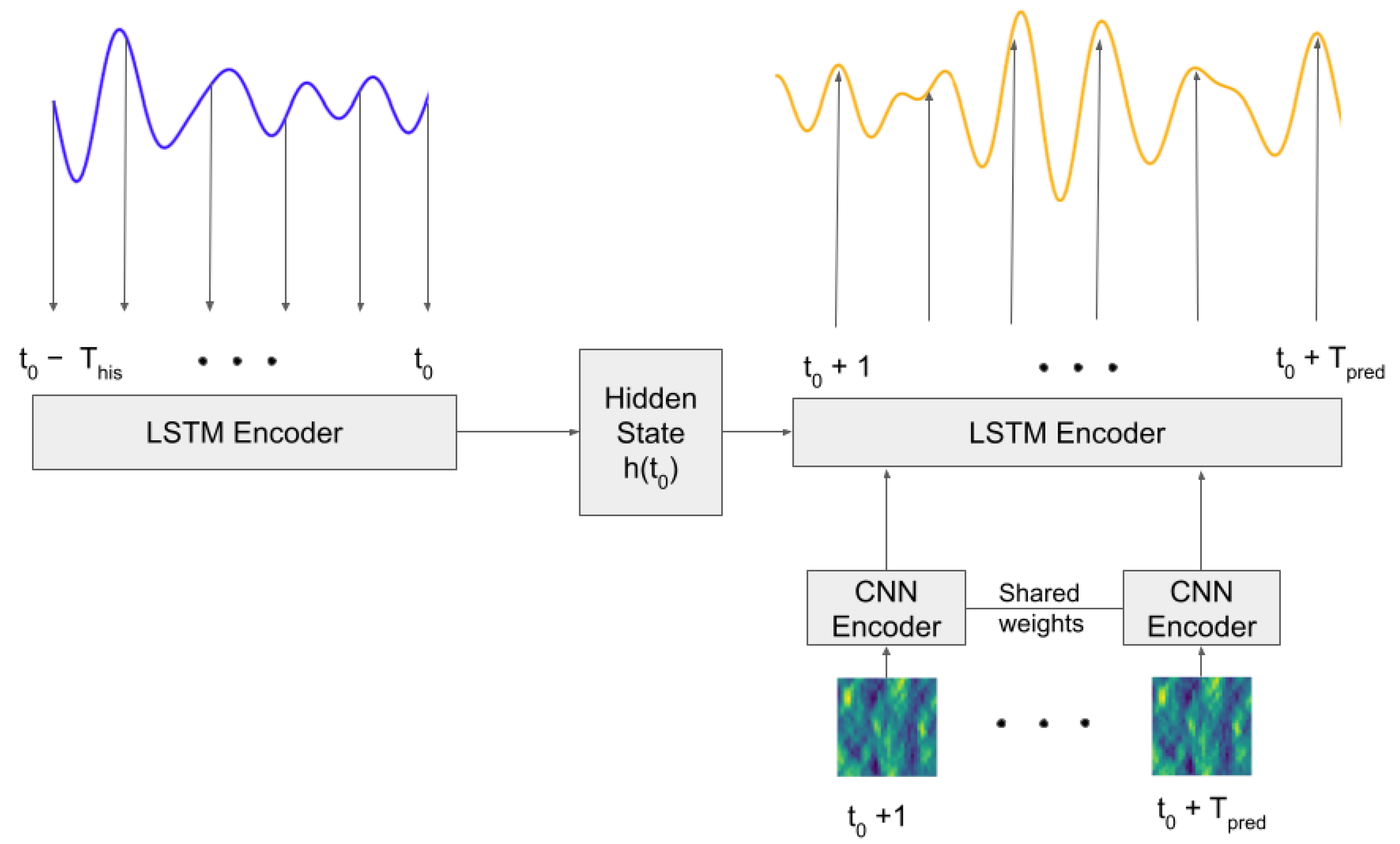
This integrated approach enables the model to simultaneously capture platform motion through the LSTM encoder while incorporating the spatial characteristics of the surrounding wave field via the CNN encoder. The decoder then synthesizes both information streams to generate predictions that account for the ship’s current dynamic state as well as upcoming wave excitations. Figure 1 provides an overview of the methodology. A recorded motion history of duration T h i s serves as input to the LSTM encoder. The hidden state of the final time step is then used to initialize the LSTM decoder, which predicts the future motion over a time window T p r e d , leveraging the encoded spatiotemporal wave-field information provided by the CNN encoder module.

2.1. LSTM Encoder

The LSTM encoder functions as a sequence-to-vector (or sequence-to-one) model that processes historical ship motion records to capture the memory effects of motion-induced radiated waves. The architecture consists of one or more LSTM layers configured to process the input sequence of past ship motion data. Each LSTM cell incorporates three gates—input, forget, and output—that regulate the flow of information, allowing the network to selectively retain or discard information across time steps. This gating mechanism is particularly effective for ship motion prediction, as it captures both short-term dependencies, such as immediate wave responses (wave-frequency oscillations), and long-term dependencies, such as sustained oscillatory motions (slow-varying oscillations).
Each Degree of Freedom (DoF) is processed using a separate architecture. The output is a fixed-length state vector—specifically the final hidden state—that encapsulates the vessel’s dynamic state. This vector serves as the initial condition for the decoder, effectively representing the cumulative memory effects of past motions.

2.2. CNN Encoder

The CNN encoder processes spatiotemporal wave-field data surrounding the vessel at each recorded time instant. Unlike traditional approaches that rely on point-based wave measurements, this architecture leverages the global spatial structure of the wave field.
The architecture comprises multiple convolutional layers, each integrated with an activation function to introduce non-linearity into the feature mapping process. These layers apply a set of learnable filters to extract dominant spatial patterns, such as wave heights, directions, and dominant frequencies. By transitioning from local to global feature extraction, the CNN generates a compressed feature vector that embodies the essential characteristics of the sea surface.
The CNN’s ability to extract hierarchical features is particularly advantageous for complex sea states, as it can identify multi-scale patterns ranging from individual wave crests to broader swell characteristics. This spatial awareness is crucial for proactively accounting for how incoming waves will translate into ship excitations.

2.3. LSTM Decoder

The LSTM decoder operates as a sequence-to-sequence generator that produces future ship motion predictions by integrating the encoded ship state and the wave-field features. It transforms these fixed-length representations into a temporal sequence, which is then mapped to the final prediction values via a Dense (fully connected) layer at each time step.
This architecture enables the model to maintain a consistent internal state while generating a series of predictions that account for both the ship’s current dynamics and future wave excitations. Consequently, the decoder learns to map the fused input features to the expected hydrodynamic response patterns of the vessel.

2.4. Loss Function

Mean Squared Error (MSE) was utilized as the loss function to train the proposed model. MSE measures the average of the squared differences between the actual vessel motion and the corresponding predictions across the entire prediction window. For a sequence of n time steps, the MSE is defined as:
MSE = 1 n i = 1 n ( Y i Y ^ i ) 2
where Y i denotes the ground-truth motion value and Y ^ i represents the predicted motion at the i-th time step. By minimizing the MSE, the model is optimized to produce trajectories that closely approximate the actual motion, thereby improving its overall regression accuracy and predictive reliability.
The three modules were jointly trained as a single end-to-end model. Training was implemented in PyTorch 1.11 using the AdamW optimizer with an initial learning rate of 10 3 and weight decay of 0.01. To ensure numerical stability, gradient clipping with a maximum norm of 1.0 was applied, effectively preventing gradient explosion, which is a common challenge in deep recurrent networks. A separate model was trained for each dataset over 200 epochs with a batch size of 32. The next section describes the characteristics of the dataset in detail.

3. Numerical Model and Collection of Synthetic Dataset

3.1. FPSO–Mooring–Riser Coupled Dynamics Simulations in a Time Domain

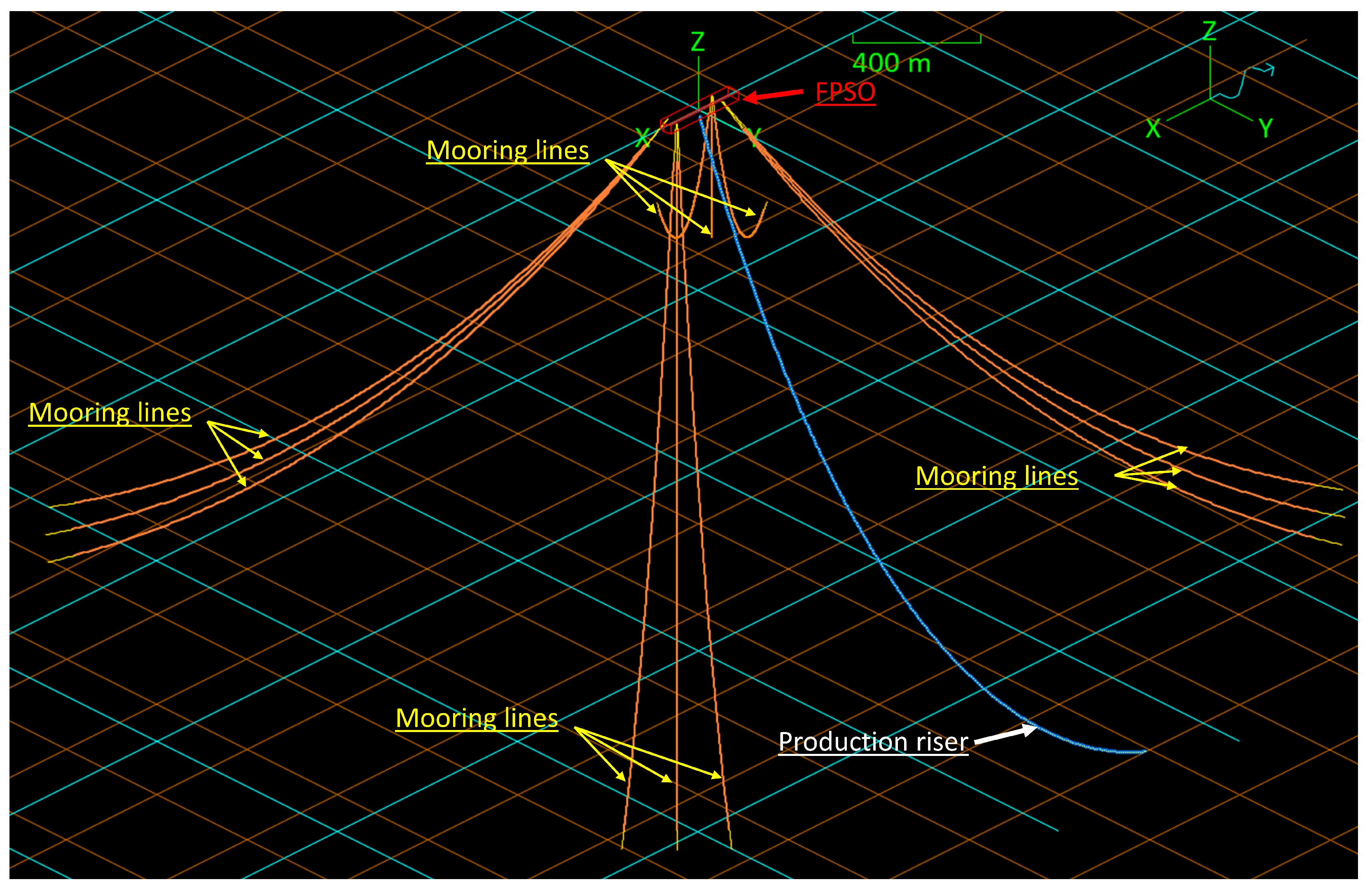
This section describes the coupled numerical model used to generate synthetic datasets, which serve as inputs and outputs for the CNN–LSTM algorithm, as well as the environmental conditions considered in this study. The FPSO vessel was modeled as a floating structure. Specifically, the FPSO unit was moored using a spread mooring system consisting of twelve lines and a single steel catenary riser, designed for operations in a water depth of 1500 m, as illustrated in Figure 2. The mooring lines were arranged into four groups, each comprising three lines in a chain–polyester–chain configuration. This study modeled a single production riser, whereas multiple risers are typically used in practice. Although this simplification may affect the overall dynamic behavior to some extent, the numerical model remains capable of capturing the representative motions of a typical FPSO, as discussed in later sections. Key specifications of the FPSO, along with details of its mooring lines and riser, are summarized in Table 1 and Table 2.
Time-domain dynamic simulations were conducted to generate time series of FPSO motions and the spatial distribution of wave elevation. The dynamic behavior of the spread-moored FPSO was analyzed using the OrcaFlex software [50], which models the coupled interactions among the FPSO, mooring lines, and production riser under various environmental conditions. The 6 DoF motions of the FPSO were computed by solving the Cummins equation [51], a widely adopted formulation in time-domain floating-body dynamics. The added mass, radiation damping, and hydrostatic stiffness matrices, along with the first-order and slowly varying wave excitation forces (the latter estimated using Newman’s approximation), were derived from frequency-domain results using a 3D diffraction/radiation solver widely used in engineering applications [52]. The mooring lines and riser were modeled using the lumped mass method to capture their elastic behavior, and the hydrodynamic forces acting on them were calculated using the Morison equation. A static simulation was first performed to define the static position under static loading, followed by a dynamic simulation under dynamic loading. Further methodological details on the dynamic simulations for this FPSO vessel can be found in Refs. [48,53].
The present generic FPSO platform was experimentally validated in a wave basin under combined wind, wave, and current conditions [54], and has subsequently been employed in numerous studies. The fidelity of line dynamics modeling in OrcaFlex has been verified through experimental results and benchmark comparisons with an in-house dynamics simulation tool [55,56].

3.2. Environmental Conditions and Collection of Synthetic Dataset

Only wave loads were considered as environmental conditions in this study, although wind and current forces can also influence the overall dynamics to some extent. Table 3 summarizes the wave conditions considered. Significant wave heights, H s , were selected to represent various sea states, each paired with a corresponding peak period, T p . Five environmental conditions were chosen to capture sea states of varying severity. Although real ocean environments often involve bidirectional waves, such as combinations of swell and wind waves, this study adopts directional head-sea wind-generated waves as a preliminary step to validate the proposed algorithm. The Pierson–Moskowitz (PM) spectrum was used as the input to generate wave elevation time series, while including directional spreading using cosign-n type spreading exponent [50]. Spatially varying wave fields were created based on the principle of superposition, in which random waves are synthesized by combining multiple sinusoids (i.e., regular waves). The equal energy method was applied, assigning each sinusoid the same spectral energy while distributing them across distinct frequency intervals to avoid repetition in the time series.
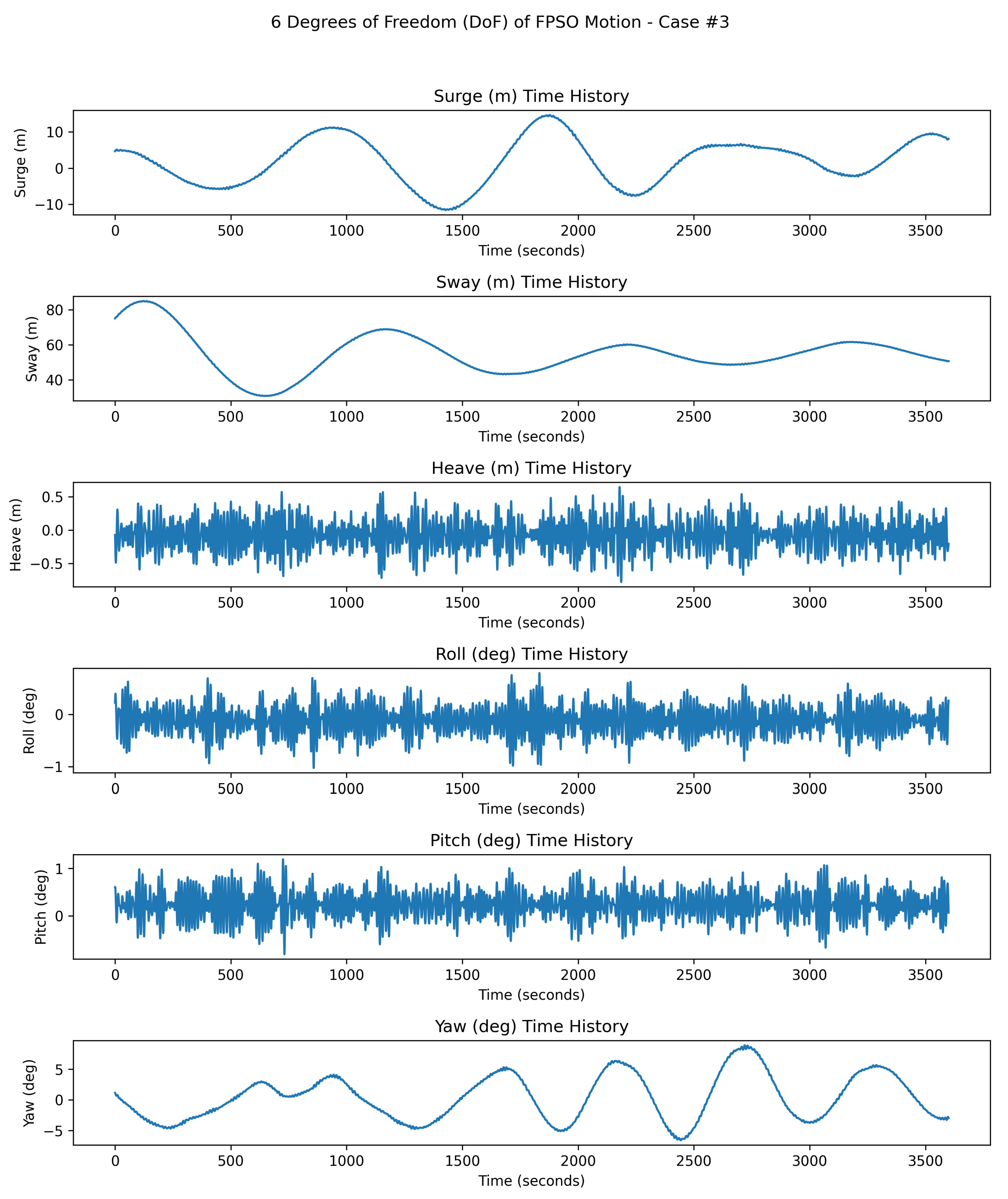
Each environmental condition case was simulated for a duration of one hour with a time step of 0.1 s (10 Hz) to ensure numerical accuracy. Figure 3 presents a representative example of the FPSO motion over the one-hour simulation period, starting from its static equilibrium position under the applied environmental load. It is worth noting that the equilibrium position in the sway direction is non-zero due to the presence of the production riser. The planar motions (surge, sway, and yaw) exhibit longer-period oscillations (slow-varying oscillations), while the non-planar motions (heave, roll, and pitch) show higher-frequency responses (wave-frequency oscillations). This behavior is typical for spread-moored FPSO systems.
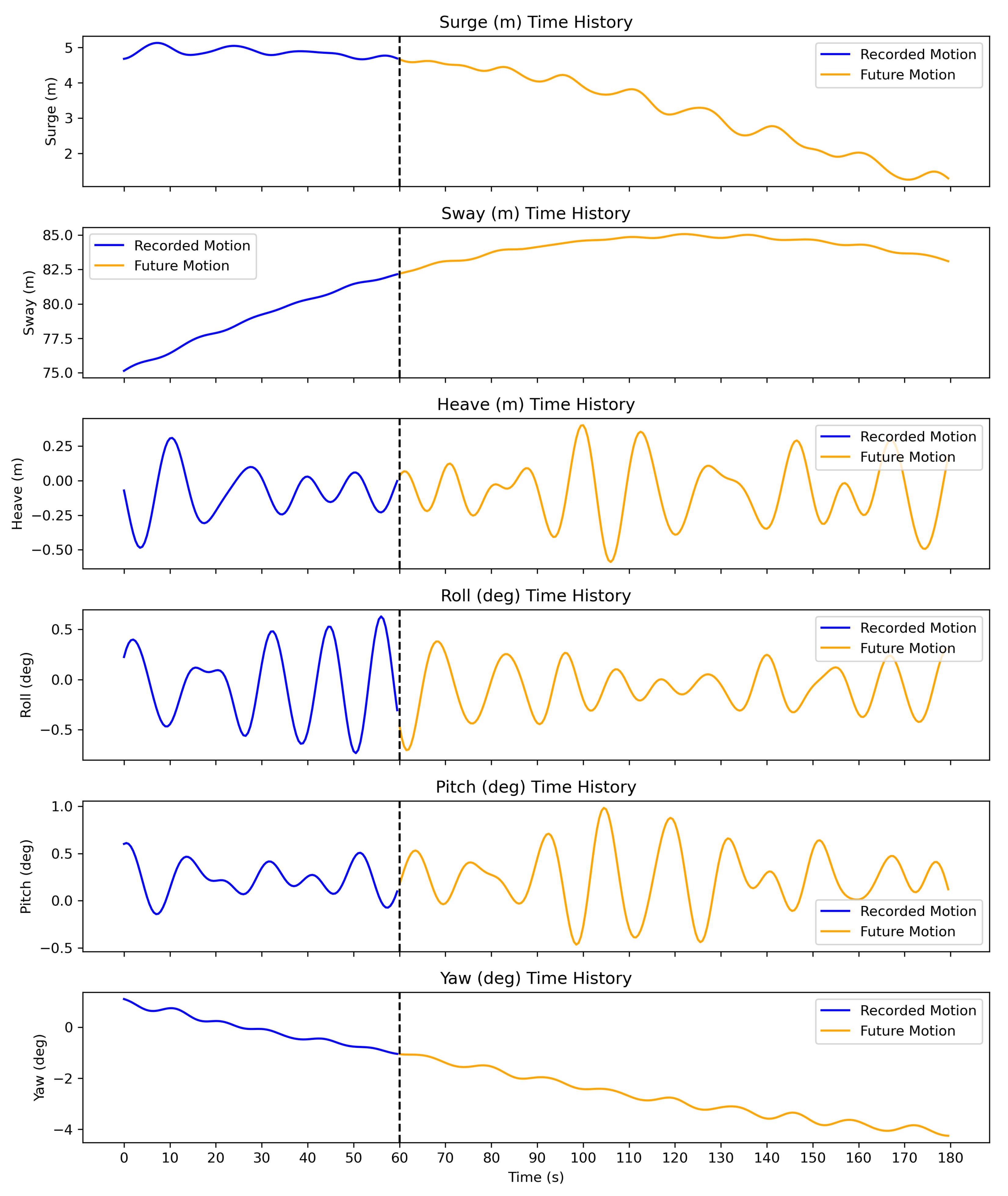
During the data collection process, measurements were sampled at a lower frequency of 2 Hz (every 0.5 s) compared to the time interval used in the dynamic simulations. The resulting 6 DoF motion displacements at the vessel’s origin (0, 0, 0) and the wave elevations at fixed coordinates in the wave field were recorded at the same sampling rate. For vessel motions, a total duration of 180 s was collected for each data point, with the initial 60 s segment used as input and the remaining 120 s used as ground-truth output. A recurrent time-window shifting technique with Δ t = 2.5 s was employed. Specifically, for the n-th dataset, the selected time window spans [ ( n 1 ) × Δ t , ( n 1 ) × Δ t + 120 ] s. This process resulted in 1380 samples for each environmental condition. The samples were then divided into training (60%), validation (20%), and test (20%) sets, which were randomly selected. An example of the input and output data for each of the 6 DoFs is illustrated in Figure 4. Additionally, wave field data were collected at the current time step, defined as ( n 1 ) × Δ t + 60 s. The spatial size of the wave field was determined based on convergence tests, the results of which are presented in Section 4.

4. Results and Discussion

This section evaluates the performance of the developed CNN–LSTM-based motion prediction algorithm. The appropriate wave field size was first determined through sensitivity tests. Subsequently, the algorithm’s performance was assessed under various wave conditions. Both statistical metrics and time-series plots are presented to support the evaluation, and the corresponding results are discussed in detail.

4.1. Selection of Wave-Field Size

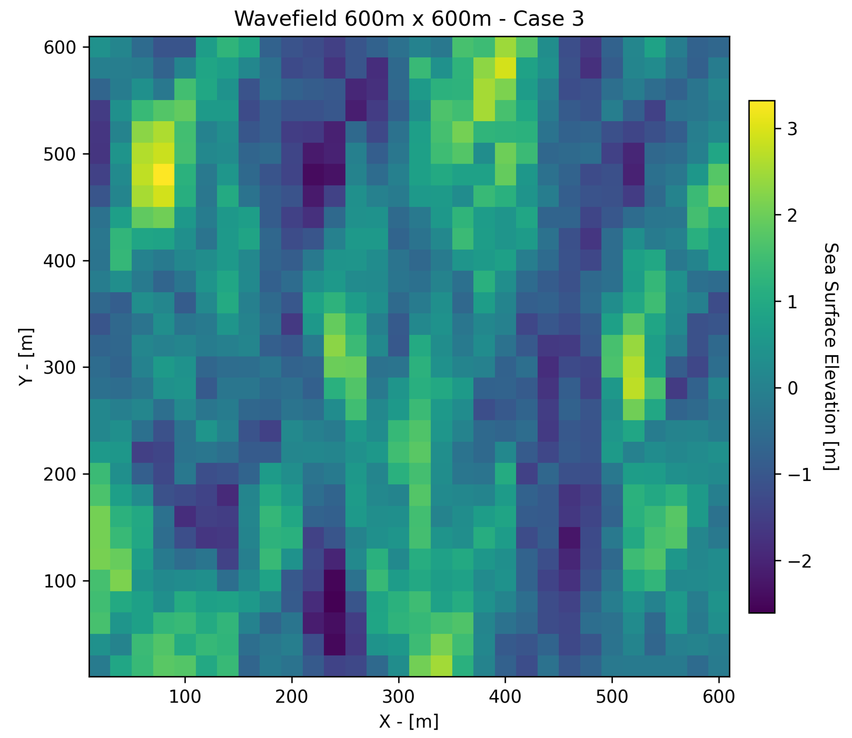
Selecting an appropriate wave-field size is a critical step in developing a cost-effective algorithm with high accuracy since the given framework typically requires real-time operations. In this problem, the computational cost of the LSTM component was relatively low compared to that of the CNN, primarily due to the large data sizes involved in CNN processing. This is particularly relevant when considering the spatial extent of the wave field in relation to the FPSO size and typical wavelengths. In this study, three wave-field sizes of 300 m × 300 m, 600 m × 600 m, and 1000 m × 1000 m were evaluated. The grid resolution was kept constant (with a fixed spatial interval of Δ x = 20 m, see Figure 5) and selected using the maximum resolution that can fit in a consumer GPU, resulting in a trade-off between wave-field resolution and computational cost. In other words, the 50 × 50 grid points of the 1000 m × 1000 m case served as the limiting factor. Finer grid points may improve accuracy, ensuring the real-time operational capability of the algorithm is a critical constraint, which ultimately determined the current grid configuration.
A convergence test was performed with respect to the field size, where an increase in field size necessitates a larger number of grid points. The third environmental condition ( H s = 4 m and T p = 12 s) was selected for this test. Specifically, a case with a larger T p was chosen because longer peak periods correspond to longer peak wavelengths, requiring a more extensive wave-field size for accurate representation. The number of LSTM layers, latent variables, CNN filters, and activation functions were optimized through trial and error. The resulting hyperparameters, which balance prediction accuracy and computational efficiency, are summarized in Table 4.
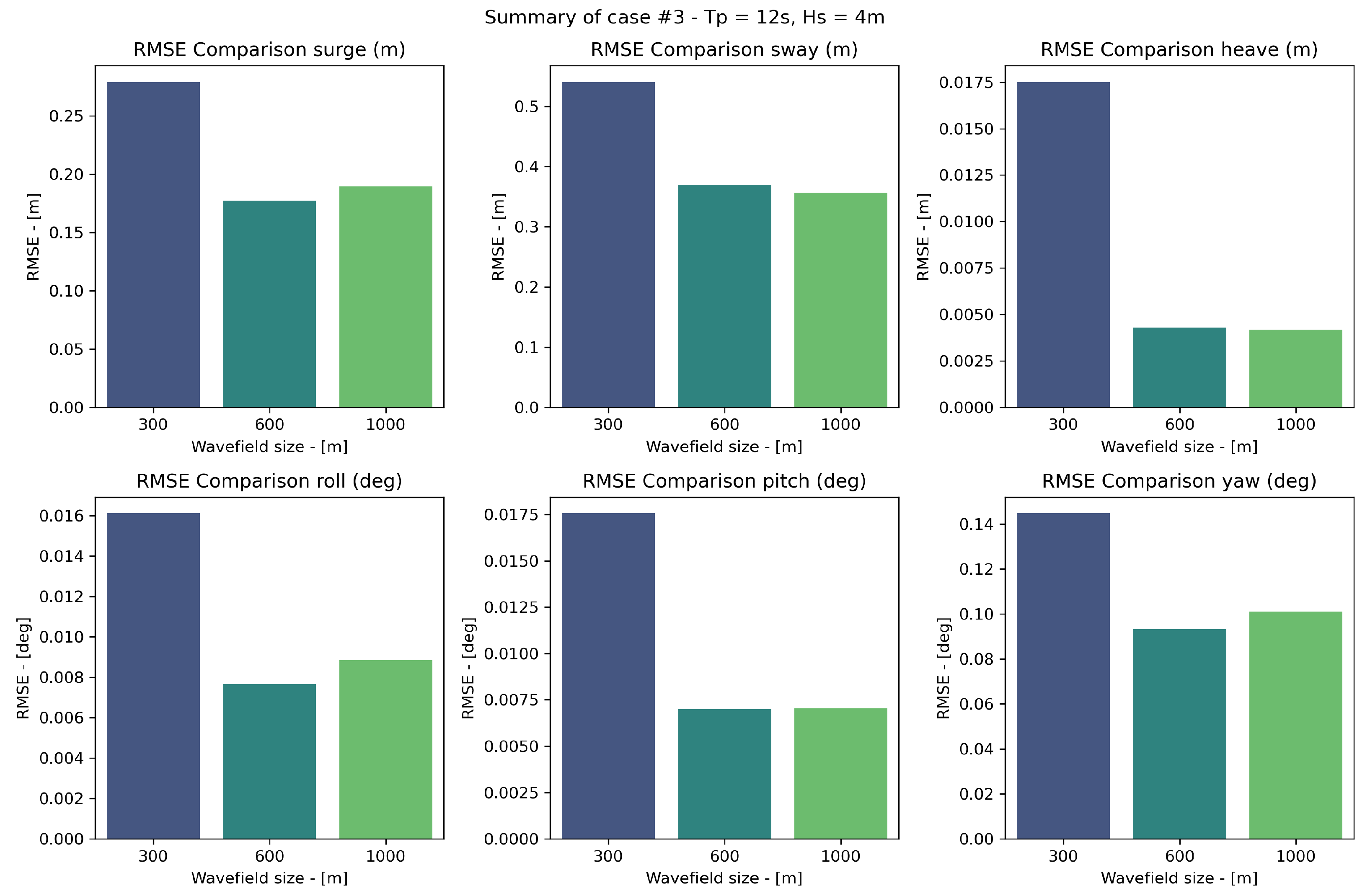
Figure 6 illustrates the Root Mean Square Error (RMSE) for the 6 DoF motions, derived from a comparative analysis between the predicted trajectories and the ground-truth data. Following the methodology described previously, the CNN–LSTM framework was employed to forecast 120 s of future ship response, utilizing a 60 s window of historical motion data coupled with the instantaneous wave-field snapshot. The prediction accuracy was quantitatively rigorously assessed using a dedicated testing dataset (20% of the total data). The results demonstrate that all evaluated configurations achieve remarkably low RMSE levels relative to the overall motion magnitudes presented in Figure 3. Notably, a critical threshold in prediction performance was observed at a wave-field size of 600 m × 600 m. This domain size—approximately twice the length of the FPSO—is sufficient to encompass the spatial characteristics of wave components with periods (T) up to 19.6 s, as calculated by the deep-water dispersion relation, L = g T 2 2 π where L is the wavelength and g is the gravity acceleration. While the 1000 m × 1000 m configuration yielded a comparable level of accuracy, no significant performance gains were observed beyond the 600 m scale. This suggests that a wave field extending twice the vessel length captures the essential spatial-temporal features required for accurate motion prediction. Consequently, the 600 m × 600 m wave field was selected as the optimal spatial input for all subsequent evaluations, as it provides the most favorable balance between predictive fidelity and computational efficiency.
It should be noted that the selected 600 m × 600 m wave-field size may exceed the practical field of view of a stereo camera. Moreover, the actual viewing area, when projected onto the horizontal plane, is not a perfect rectangle but more closely resembles a curved trapezoid. As this study serves as an initial assessment of the proposed CNN–LSTM algorithm, future work will incorporate detailed modeling of the stereo camera’s geometry and optical characteristics to further evaluate the system’s practical feasibility. The second author’s research group has already developed a wave-field estimator using stereo cameras [44], which can be readily integrated in future studies.

4.2. Performance in Different Wave Conditions

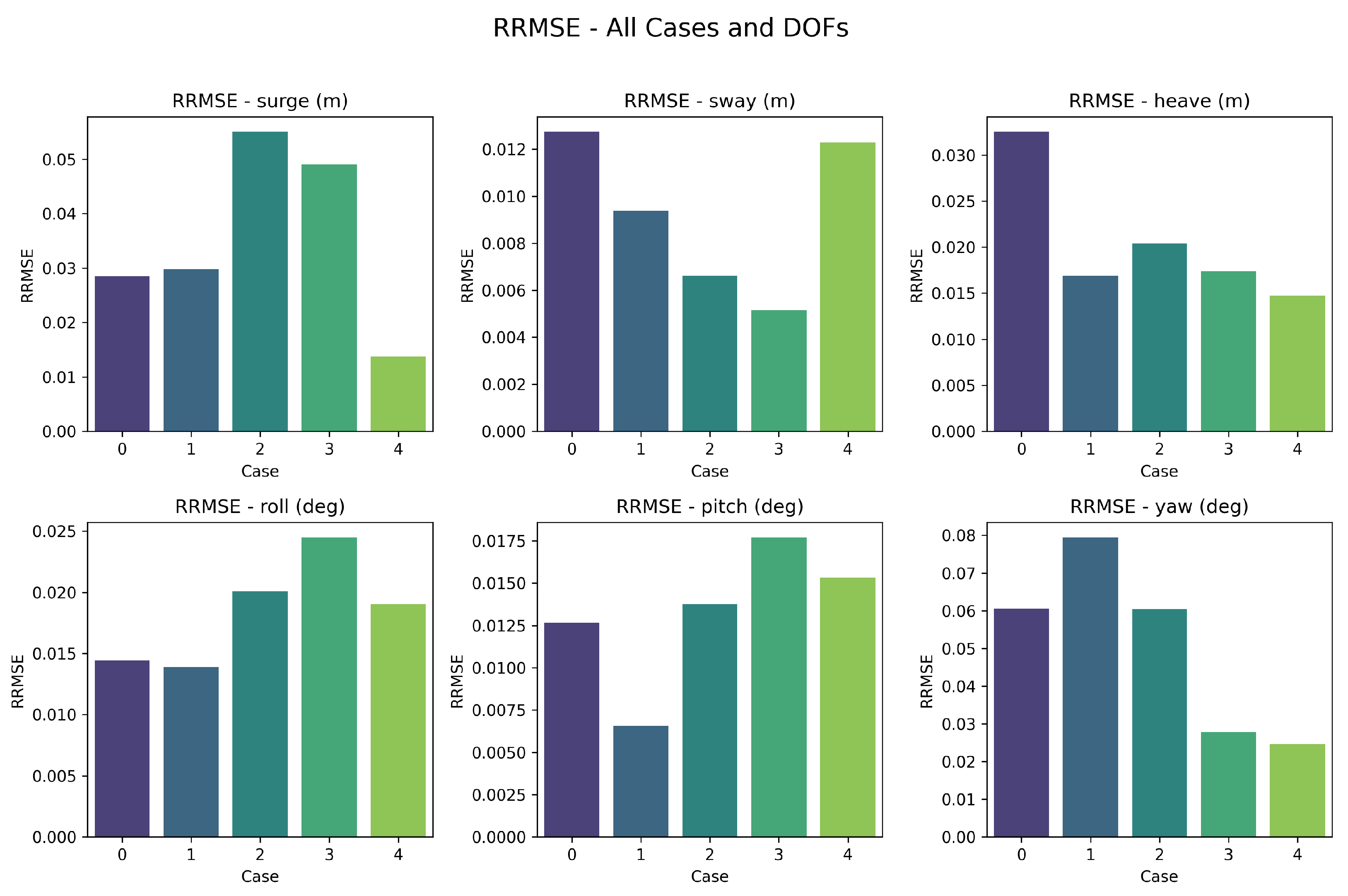
In this section, we evaluate the performance of the proposed CNN-LSTM algorithm across all defined environmental conditions, ranging from the calmest (Case 0) to the most severe (Case 4) sea states. To normalize the varying motion amplitudes, the Relative Root Mean Squared Error (RRMSE) was utilized, which is calculated by dividing the RMSE by the root mean square of the predicted motion values. This approach allows for a consistent comparison of predictive accuracy regardless of the magnitude of the vessel’s response.
As summarized in Figure 7, the RRMSE values exhibit distinct behaviors depending on the DoFs. For the primarily oscillatory motions (non-planar motions)—heave, roll, and pitch—the RRMSE values remain consistently low and show a relatively stable trend across all sea states. This is particularly evident in heave, where the RRMSE is maintained within a narrow range between 0.015 and 0.032 from Case 0 to Case 4. In contrast, the horizontal motions (planar motions)—surge, sway, and yaw—exhibit relatively higher RRMSE values and a lack of clear trends due to their low-frequency, slow-varying nature. In the absence of wind, these motions are primarily driven by second-order wave drift forces and the restorative dynamics of the mooring and riser systems, rather than the first-order wave excitation that governs heave, roll, and pitch. These horizontal responses are, thus, less directly coupled with the instantaneous wave-field snapshots provided to the CNN, as they represent an integrated response to wave energy over time. Consequently, the predictions do not show a clear trend with sea state severity and are more likely to include unpredictable errors.
The difference in prediction performance between planar and non-planar motions is linked to the specific roles of the CNN and LSTM encoders. Heave, roll, and pitch are primarily driven by wave-frequency excitations, where both the CNN (capturing the wave field) and LSTM (tracking motion history) play significant roles. Conversely, surge, sway, and yaw are heavily governed by low-frequency mooring dynamics. In these horizontal motions, the LSTM encoder becomes the dominant factor for estimation, while the CNN encoder plays a peripheral role. This distinction highlights why integrating both CNN and LSTM algorithms is essential, particularly for non-planar motions, rather than relying solely on a standard LSTM approach.
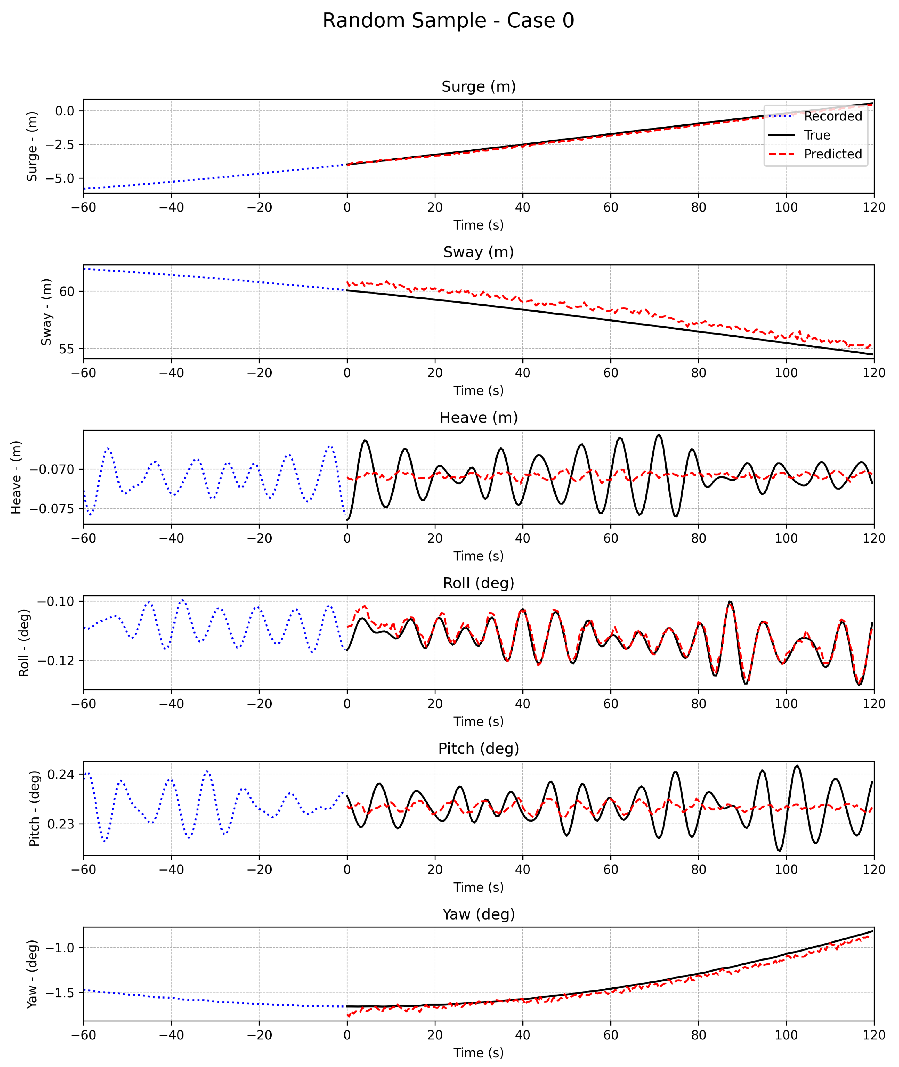
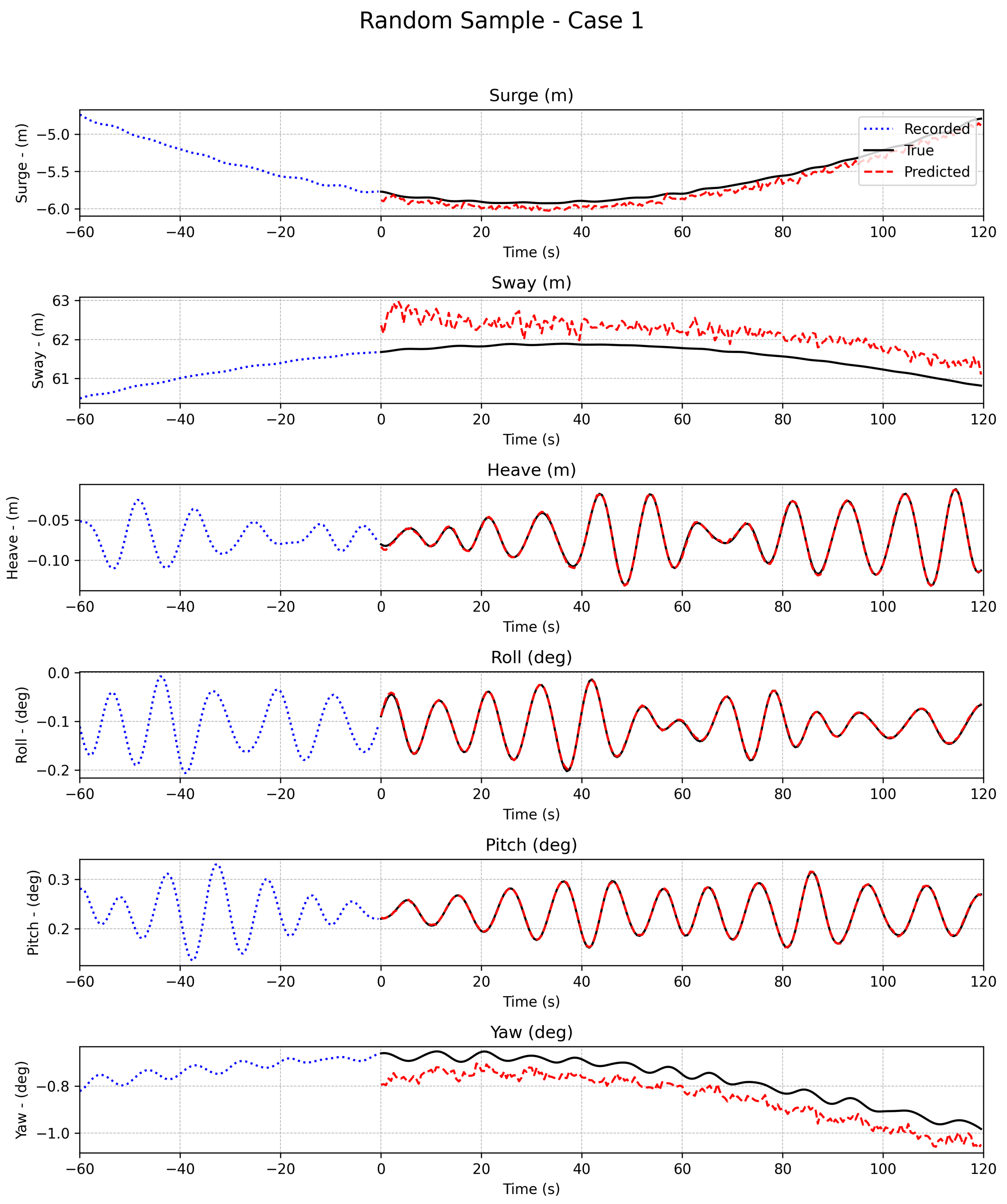
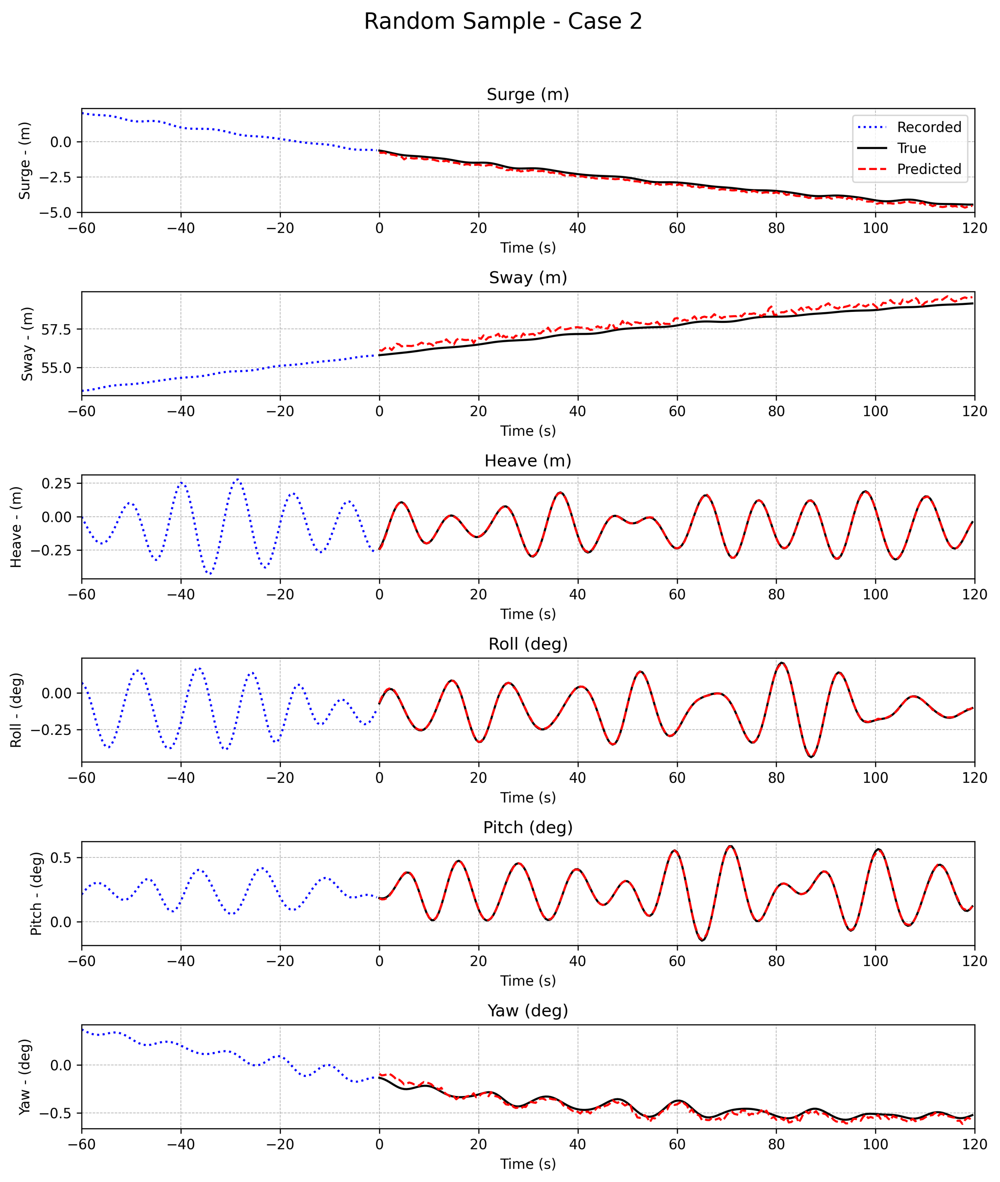
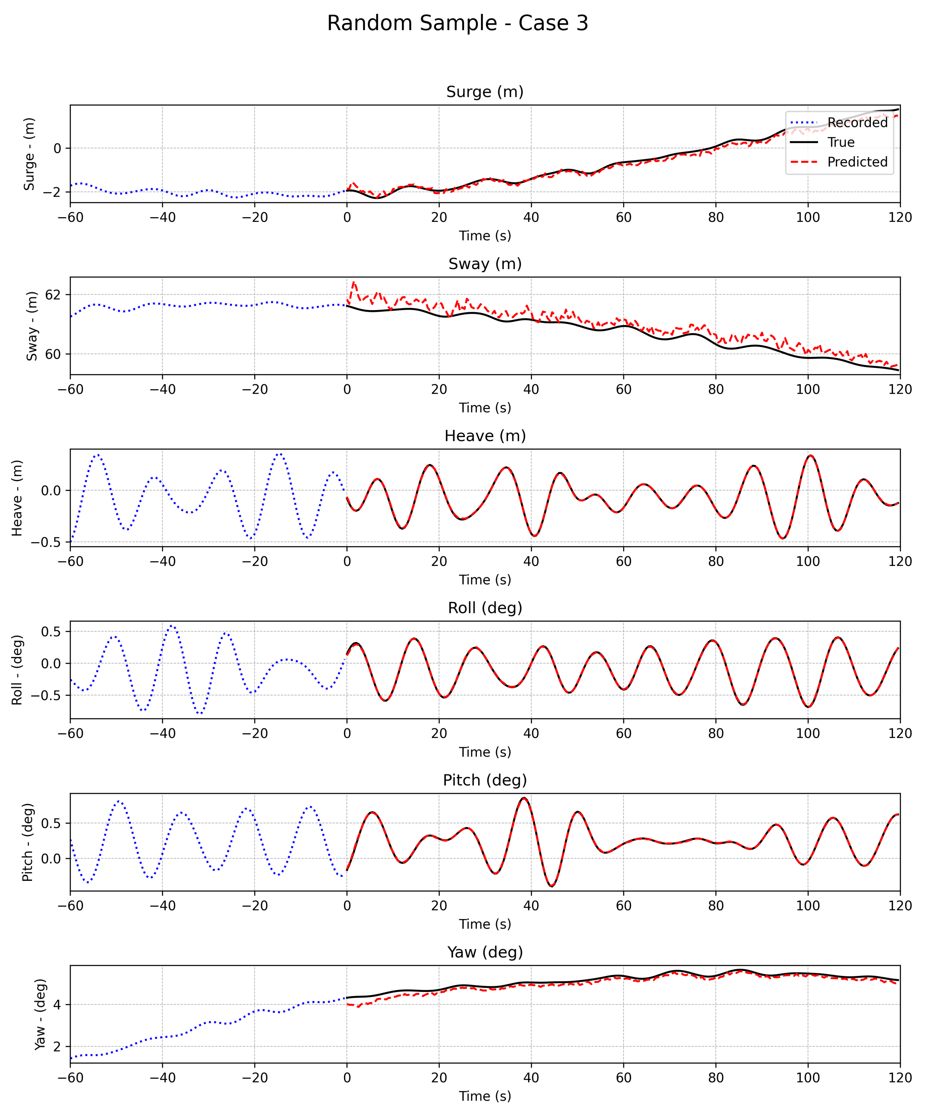
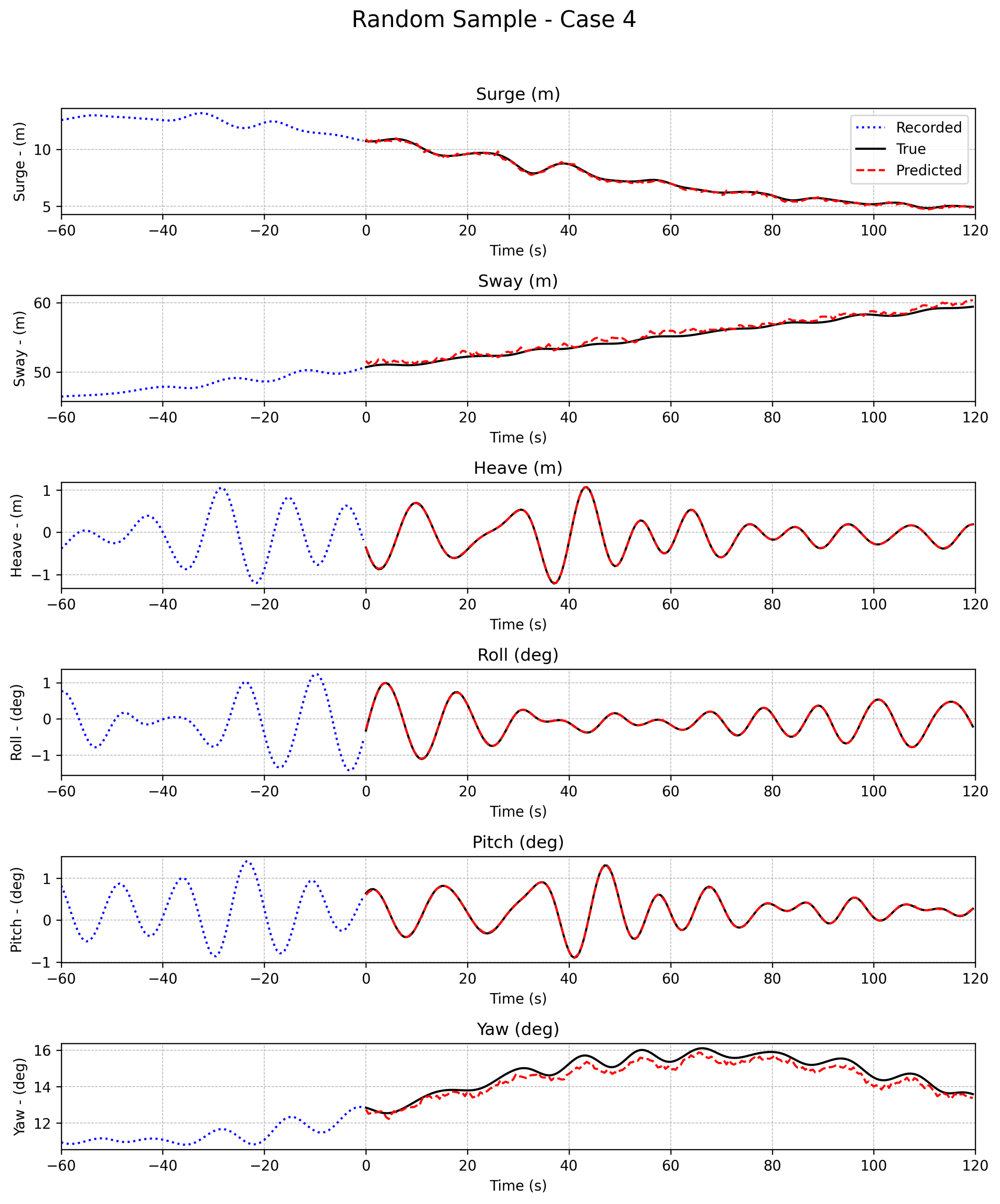
Qualitatively, the time–history plots present an important contrast to these numerical trends, as shown in Figure 8, Figure 9, Figure 10, Figure 11 and Figure 12. The snapshots presented therein were randomly selected from the testing dataset to ensure an unbiased representation of the model’s performance. However, the given time history plots are representative cases, making it difficult to represent the overall statistical data given in Figure 7. In Case 0, despite achieving the low RRMSE values for the vertical motions, the predicted signals in Figure 8 appear noisier and show less precise phase tracking. This visual discrepancy arises because the absolute motion magnitude is extremely small; even minor numerical fluctuations appear as prominent jitter in the time–history plot while remaining mathematically insignificant in the RRMSE calculation. Conversely, in Case 4 (Figure 12), the model demonstrates robust prediction for high-amplitude dynamics. The model successfully captures the nonlinear, high-amplitude dynamics with smooth transitions and synchronized phases, as the higher-energy content in severe sea states provides a more robust dynamic signature for the LSTM to learn.
As shown in the time–history plots, the slow-varying nature of planar motions suggests that the current dataset may not be sufficient in volume to fully capture these long-period characteristics. The complexity of surge, sway, and yaw requires a more extensive amount of training data to improve the model’s generalization for low-frequency dynamics. Future work will focus on expanding the total dataset size and conducting a convergence analysis to ensure that the model is provided with enough samples to learn the low-frequency behaviors of the system.
In summary, the model achieves high predictive accuracy with consistently low RRMSE values across most sea states. However, these numerical metrics do not always align with the qualitative behavior, as predicted signals in low sea states often show numerical jitter and phase lags despite having the smallest RRMSE. In contrast, the model performs better in high-amplitude conditions where stronger dynamic signatures allow for more synchronized predictions. For planar motions, the predictions are generally noisier and lack clear trends due to their complex, low-frequency dynamics.

5. Concluding Remarks

This study developed and validated a CNN–LSTM hybrid deep learning framework to predict the dynamic motions of a moored FPSO vessel using synthetic wave and motion datasets. The architecture is composed of three core components: an LSTM encoder to capture historical motion memory, a CNN encoder to extract spatial features from the surrounding wave field, and an LSTM decoder that integrates these features to generate multistep future motion predictions.
The numerical datasets were generated through mid-fidelity time-domain simulations in OrcaFlex, incorporating full 6 DoF dynamics, mooring lines, and risers under different wave conditions. Through extensive hyperparameter tuning and wave-field convergence tests, several key findings were obtained:
  • A wave-field size of 600 m × 600 m (approximately twice the vessel length) was identified as the optimal spatial input, providing the best balance between computational efficiency and predictive accuracy.
  • The model demonstrated superior qualitative fidelity in higher sea states (e.g., H s = 7 m). The predictions were smoother and more synchronized due to the larger dynamic motions. Conversely, low sea states presented small-amplitude signals that were more susceptible to numerical noise and phase-tracking lag.
  • While wave-excited motions (heave, roll, pitch) achieved consistently high precision across all sea states, horizontal motions (surge, sway, yaw) remained more difficult to predict due to their slow-varying nature governed by second-order drift forces and mooring dynamics.
  • The CNN–LSTM architecture successfully fused spatial wave-field features with temporal motion sequences, enabling robust performance across all tested environments.
As an initial step, this study demonstrates the feasibility of utilizing CNN–LSTM-based frameworks for real-time motion prediction in offshore environments. Future work will extend this framework by replacing the idealized spatial wave inputs with real-time wave fields estimated from stereo camera imagery. This integrated system will undergo rigorous validation in synthetic environments before proceeding to actual sea trials. Ultimately, we aim to deploy this predictive intelligence into real-world offshore operations, where it can serve as a critical tool for enhancing operational safety and decision-making efficiency. By providing reliable motion forecasts, the proposed model is expected to support a wide range of practical applications.

Author Contributions

Conceptualization, C.J.; methodology, O.J., C.J. and B.K.; software, O.J., C.J. and S.H.H.; validation, O.J., C.J., S.H.H. and B.K.; formal analysis, O.J., C.L. and Y.H.J.; investigation, B.K. and C.L.; resources, O.J.; data curation, O.J.; writing—original draft preparation, O.J.; writing—review and editing, C.J., B.K., S.H.H. and Y.H.J.; visualization, O.J.; supervision, C.J.; project administration, C.L.; funding acquisition, C.L. All authors have read and agreed to the published version of the manuscript.

Funding

This research was supported by the Ministry of SMEs and Startups (MSS), Korea Institute for Advancement of Technology (KIAT) through the Innovation Development (R&D) for Global Regulation-Free Special Zone [GRANT Number: RS-2024-00488440].

Data Availability Statement

The raw data supporting the conclusions of this article will be made available by the authors upon request.

Conflicts of Interest

The authors declare no conflicts of interest.

References

  1. Sun, Q.; Tang, Z.; Gao, J.; Zhang, G. Short-term ship motion attitude prediction based on LSTM and GPR. Appl. Ocean Res. 2022, 118, 102927. [Google Scholar] [CrossRef]
  2. Yang, Y.; Peng, T.; Liao, S. Predicting 3-DoF motions of a moored barge by machine learning. J. Ocean Eng. Sci. 2023, 8, 336–343. [Google Scholar] [CrossRef]
  3. Li, N.; Zou, G.; Feng, Y.; Ali, L. Probabilistic Prediction of Floating Offshore Wind Turbine Platform Motions via Uncertainty Quantification and Information Integration. J. Mar. Sci. Eng. 2024, 12, 886. [Google Scholar] [CrossRef]
  4. Pan, W.; Guo, X.; Li, X. Benchmark Dataset for Offshore Platform Motion Prediction and Its Applications. J. Mar. Sci. Eng. 2024, 12, 1852. [Google Scholar] [CrossRef]
  5. Li, G.; Zhang, H.; Kawan, B.; Wang, H.; Osen, O.L.; Styve, A. Analysis and modeling of sensor data for ship motion prediction. In Proceedings of the OCEANS 2016-Shanghai; IEEE: New York, NY, USA, 2016; pp. 1–7. [Google Scholar]
  6. Zhang, D.; Chu, X.; Liu, C.; He, Z.; Zhang, P.; Wu, W. A Review on Motion Prediction for Intelligent Ship Navigation. J. Mar. Sci. Eng. 2024, 12, 107. [Google Scholar] [CrossRef]
  7. Skulstad, R.; Li, G.; Fossen, T.I.; Vik, B.; Zhang, H. A hybrid approach to motion prediction for ship docking—Integration of a neural network model into the ship dynamic model. IEEE Trans. Instrum. Meas. 2020, 70, 2501311. [Google Scholar] [CrossRef]
  8. Zhang, T.; Zheng, X.Q.; Liu, M.X. Multiscale attention-based LSTM for ship motion prediction. Ocean Eng. 2021, 230, 109066. [Google Scholar] [CrossRef]
  9. Liu, Y.; Yuan, H.; Xiao, Z.; Xiao, C. An Offshore Self-Stabilized System Based on Motion Prediction and Compensation Control. J. Mar. Sci. Eng. 2023, 11, 745. [Google Scholar] [CrossRef]
  10. Zhao, M.; Zheng, X.Y.; Zhang, S.; Qian, K.; Jiang, Y.; Liu, Y.; Duan, M.; Zhao, T.; Zhai, K. Hydrodynamic Performance and Motion Prediction Before Twin-Barge Float-Over Installation of Offshore Wind Turbines. J. Mar. Sci. Eng. 2025, 13, 995. [Google Scholar] [CrossRef]
  11. Zhang, X.; Ji, R.; Sun, K.; Zhang, J.; Zhang, X.; Yin, M.; Kong, M.; Reabroy, R. A review of ocean tidal current energy technology: Advances, trends, and challenges. Phys. Fluids 2025, 37, 071308. [Google Scholar] [CrossRef]
  12. Kong, M.; Zhang, X.; Ji, R.; Wu, H.; Yin, M.; Liu, H.; Sun, K.; Reabroy, R. Effects of wave–current interaction on hydrodynamic performance and motion response of a floating tidal stream turbine. J. Mar. Sci. Eng. 2025, 13, 1520. [Google Scholar] [CrossRef]
  13. Jin, C.; Kang, H.; Kim, M.; Cho, I. Performance estimation of resonance-enhanced dual-buoy wave energy converter using coupled time-domain simulation. Renew. Energy 2020, 160, 1445–1457. [Google Scholar] [CrossRef]
  14. Küchler, S.; Mahl, T.; Neupert, J.; Schneider, K.; Sawodny, O. Active control for an offshore crane using prediction of the vessel’s motion. IEEE/ASME Trans. Mechatron. 2010, 16, 297–309. [Google Scholar] [CrossRef]
  15. Chu, Y.; Li, G.; Zhang, H. Incorporation of ship motion prediction into active heave compensation for offshore crane operation. In Proceedings of the 2020 15th IEEE Conference on Industrial Electronics and Applications (ICIEA), Kristiansand, Norway, 9–13 November 2020; pp. 1444–1449. [Google Scholar]
  16. Yin, J.; Ding, J.; Yang, Y.; Yu, J.; Ma, L.; Xie, W.; Nie, D.; Bashir, M.; Liu, Q.; Li, C.; et al. Wave-induced motion prediction of a deepwater floating offshore wind turbine platform based on Bi-LSTM. Ocean Eng. 2025, 315, 119836. [Google Scholar] [CrossRef]
  17. Song, S.S.; Kim, S.H.; Kim, H.S.; Jeon, M.R. A study on the feedforward control algorithm for dynamic positioning system using ship motion prediction. J. Korean Soc. Mar. Environ. Saf. 2016, 22, 129–137. [Google Scholar] [CrossRef]
  18. Cademartori, G.; Oneto, L.; Valdenazzi, F.; Coraddu, A.; Gambino, A.; Anguita, D. A review on ship motions and quiescent periods prediction models. Ocean Eng. 2023, 280, 114822. [Google Scholar] [CrossRef]
  19. Kaplan, P. A study of prediction techniques for aircraft carrier motions at sea. J. Hydronautics 1969, 3, 121–131. [Google Scholar] [CrossRef]
  20. Connell, B.S.; Rudzinsky, J.P.; Brundick, C.S.; Milewski, W.M.; Kusters, J.G.; Farquharson, G. Development of an environmental and ship motion forecasting system. In Proceedings of the International Conference on Offshore Mechanics and Arctic Engineering; American Society of Mechanical Engineers: New York, NY, USA, 2015; Volume 56598, p. V011T12A058. [Google Scholar]
  21. Triantafyllou, M.; Athans, M. Real time estimation of the heaving and pitching motions of a ship, using a Kalman filter. In Proceedings of the OCEANS 81; IEEE: New York, NY, USA, 1981; pp. 1090–1095. [Google Scholar]
  22. Lavrov, A.; Rodrigues, J.; Gadelho, J.; Soares, C.G. Calculation of hydrodynamic coefficients of ship sections in roll motion using Navier-Stokes equations. Ocean Eng. 2017, 133, 36–46. [Google Scholar] [CrossRef]
  23. La Ferlita, A.; Ley, J.; Qi, Y.; Schellin, T.E.; Di Nardo, E.; El Moctar, O.; Ciaramella, A. Data-driven model assessment: A comparative study for ship response determination. Ocean Eng. 2024, 314, 119711. [Google Scholar] [CrossRef]
  24. Ferlita, L.; La, A. Assessment of Data-Driven Model for the Prediction of Ship Performances and Responses. Ph.D. Thesis, Universität Duisburg-Essen, Duisburg/Essen, Germany, 2025. [Google Scholar]
  25. Skulstad, R.; Li, G.; Fossen, T.I.; Wang, T.; Zhang, H. A co-operative hybrid model for ship motion prediction. Mode. Identif. Control 2021, 42, 17–26. [Google Scholar] [CrossRef]
  26. Li, X.; Lv, X.; Yu, J.; Li, J. Neural network application on ship motion prediction. In Proceedings of the 2017 9th International Conference on Intelligent Human-Machine Systems and Cybernetics (IHMSC), Hangzhou, China, 26–27 August 2017; Volume 1, pp. 414–417. [Google Scholar]
  27. Alvarellos, A.; Figuero, A.; Sande, J.; Peña, E.; Rabuñal, J. Deep learning based ship movement prediction system architecture. In Proceedings of the International Work-Conference on Artificial Neural Networks; Springer: Berlin/Heidelberg, Germany, 2019; pp. 844–855. [Google Scholar]
  28. Hu, X.; Zhang, B.; Tang, G. Research on ship motion prediction algorithm based on dual-pass long short-term memory neural network. IEEE Access 2021, 9, 28429–28438. [Google Scholar]
  29. Jiang, Y.; Hou, X.R.; Wang, X.G.; Wang, Z.H.; Yang, Z.L.; Zou, Z.J. Identification modeling and prediction of ship maneuvering motion based on LSTM deep neural network. J. Mar. Sci. Technol. 2022, 27, 125–137. [Google Scholar] [CrossRef]
  30. Lin, Z.; Yue, W.; Huang, J.; Wan, J. Ship trajectory prediction based on the TTCN-attention-GRU model. Electronics 2023, 12, 2556. [Google Scholar] [CrossRef]
  31. Hou, X.; Xia, S. Short-term prediction of ship roll motion in waves based on convolutional neural network. J. Mar. Sci. Eng. 2024, 12, 102. [Google Scholar] [CrossRef]
  32. Shi, W.; Guo, Z.; Chen, M.; Li, S.; Hu, J.; Dai, Z. Multi-step prediction of ship heave motion using transformer-enhanced multi-scale CNN. Measurement 2025, 242, 115787. [Google Scholar]
  33. Hochreiter, S. Long Short-Term Memory; Neural Computation MIT-Press: Cambridge, MA, USA, 1997. [Google Scholar]
  34. Tian, X.; Song, Y. Machine learning for short-term prediction of ship motion combined with wave input. Appl. Sci. 2023, 13, 5298. [Google Scholar] [CrossRef]
  35. Liu, Y.; Duan, W.; Huang, L.; Duan, S.; Ma, X. The input vector space optimization for LSTM deep learning model in real-time prediction of ship motions. Ocean Eng. 2020, 213, 107681. [Google Scholar] [CrossRef]
  36. Guo, X.; Zhang, X.; Lu, W.; Tian, X.; Li, X. Real-time prediction of 6-DOF motions of a turret-moored FPSO in harsh sea state. Ocean Eng. 2022, 265, 112500. [Google Scholar]
  37. Deng, Y.; Feng, W.; Xu, S.; Chen, X.; Wang, B. A novel approach for motion predictions of a semi-submersible platform with neural network. J. Mar. Sci. Technol. 2021, 26, 883–895. [Google Scholar] [CrossRef]
  38. Shi, W.; Hu, L.; Lin, Z.; Zhang, L.; Wu, J.; Chai, W. Short-term motion prediction of floating offshore wind turbine based on muti-input LSTM neural network. Ocean Eng. 2023, 280, 114558. [Google Scholar]
  39. Deng, S.; Ning, D.; Mayon, R. The motion forecasting study of floating offshore wind turbine using self-attention long short-term memory method. Ocean Eng. 2024, 310, 118709. [Google Scholar] [CrossRef]
  40. Dannenberg, J.; Reichert, K.; van den Boom, H. Wave profiles derived from nautical X-band radar as data source for ship motion prediction. In Proceedings of the 11th International Workshop on Wave Hindcasting & Forecasting, Halifax, NS, Canada, 18–23 October 2009. [Google Scholar]
  41. Guo, X.; Zhang, X.; Tian, X.; Li, X.; Lu, W. Predicting heave and surge motions of a semi-submersible with neural networks. Appl. Ocean Res. 2021, 112, 102708. [Google Scholar] [CrossRef]
  42. Guo, X.; Zhang, X.; Tian, X.; Lu, W.; Li, X. Probabilistic prediction of the heave motions of a semi-submersible by a deep learning model. Ocean Eng. 2022, 247, 110578. [Google Scholar] [CrossRef]
  43. Lee, J.H.; Lee, J.; Kim, Y.; Ahn, Y. Prediction of wave-induced ship motions based on integrated neural network system and spatiotemporal wave-field data. Phys. Fluids 2023, 35, 097127. [Google Scholar]
  44. Jebari, O.; Hong, S.H.; Hunsucker, T.; Kim, D.K.; Jin, C. Wave-field reconstruction using stereo cameras on a floating platform in a synthetic environment. Ocean Eng. 2025, 327, 120958. [Google Scholar] [CrossRef]
  45. Jung, K.H.; Lee, J.H. Experimental study on predicting the corrosion behavior of carbon steel in various corrosive environments using artificial neural networks. J. Adv. Mar. Eng. Technol. 2023, 47, 317–324. [Google Scholar]
  46. Min, S.; Jeong, K.; Noh, Y.; Won, D.; Kim, S. Damage detection for tethers of submerged floating tunnels based on convolutional neural networks. Ocean Eng. 2022, 250, 111048. [Google Scholar] [CrossRef]
  47. Sivaprasad, H.; Lekkala, M.R.; Latheef, M.; Seo, J.; Yoo, K.; Jin, C.; Kim, D.K. Fatigue damage prediction of top tensioned riser subjected to vortex-induced vibrations using artificial neural networks. Ocean Eng. 2023, 268, 113393. [Google Scholar] [CrossRef]
  48. Jebari, O.; Kwon, D.S.; Kim, S.J.; Jin, C.; Kim, M. Machine Learning-Based Mooring Failure Detection for FPSOs: A Two-Step ANN Approach. J. Mar. Sci. Eng. 2025, 13, 791. [Google Scholar]
  49. Kwon, D.S.; Kim, S.J.; Jin, C.; Kim, M.; Guha, A.; Esenkov, O.E.; Ryu, S. Inverse estimation of a vertical current velocity profile using motions of an FPSO and artificial neural network. Ocean Eng. 2023, 285, 115343. [Google Scholar] [CrossRef]
  50. Orcina Ltd. OrcaFlex Documentation, Version 11.4a; Orcina Ltd.: Ulverston, UK, 2023.
  51. Cummins, W. The Impulse Response Function and Ship Motion; Report 1661, Department of the Navy, David W. Taylor Model Basin, Hydromechanics Laboratory, Research and Development Report; October 1962; Available online: https://dome.mit.edu/bitstream/handle/1721.3/49049/DTMB_1962_1661.pdf (accessed on 1 February 2026).
  52. Jo, J.S. Study of hydrodynamic analysis of eco-friendly buoys with biodegradable plastic materials. J. Adv. Mar. Eng. Technol. (JAMET) 2023, 47, 231–237. [Google Scholar] [CrossRef]
  53. Jin, C.; Kim, S.J.; Kim, M.; Lee, Y.; Guha, A.; Ryu, S.; Xu, W. Real-time dynamic and structural behavior estimation of a steel lazy wave riser through finite-element-based digital twin and hull-motion sensor. Appl. Ocean Res. 2024, 150, 104137. [Google Scholar]
  54. Kim, M.; Koo, B.; Mercier, R.; Ward, E. Vessel/mooring/riser coupled dynamic analysis of a turret-moored FPSO compared with OTRC experiment. Ocean Eng. 2005, 32, 1780–1802. [Google Scholar]
  55. Lee, J.; Jin, C.; Kim, M. Dynamic response analysis of submerged floating tunnels by wave and seismic excitations. Ocean Syst. Eng. 2017, 7, 1–19. [Google Scholar] [CrossRef]
  56. Jin, C.; Bakti, F.P.; Kim, M. Time-domain coupled dynamic simulation for SFT-mooring-train interaction in waves and earthquakes. Mar. Struct. 2021, 75, 102883. [Google Scholar] [CrossRef]
Figure 1. Overview of the model architecture, showing the LSTM encoder/decoder and the CNN encoder.
Jmse 14 00531 g001
Figure 2. 3D view of coupled system of FPSO, mooring lines, and riser in OrcaFlex [48].
Jmse 14 00531 g002
Figure 3. 6 DoF motion displacements of FPSO over one hour, excluding ramping time and with respect to global coordinate system (0, 0, 0) for Case 3 ( H s = 4 m and T p = 12 s).
Jmse 14 00531 g003
Figure 4. Input and output sample showing the recorded motion and the future motion for all 6 DoFs. In legend, ‘Recorded Motion’ denotes input to the CNN–LSTM algorithm and ‘Future Motion’ is ground-truth output, which is compared with the predicted motion resulting from the proposed CNN-LSTM algorithm.
Jmse 14 00531 g004
Figure 5. Representative wavefield sample from Case 3 ( H s = 4 m, T p = 12 s) with Δ x = 20 m and a field size of 600 m × 600 m (30 × 30 grid points).
Jmse 14 00531 g005
Figure 6. RMSE comparison of 6 DoF motions at different wave field sizes (300 m × 300 m, 600 m × 600 m, 1000 m × 1000 m) under Case 3 wave condition ( H s = 4 m, T p = 12 s).
Jmse 14 00531 g006
Figure 7. Performance comparison at different sea state conditions: Case 0 representing the calmest sea state and Case 4 representing the highest sea state.
Jmse 14 00531 g007
Figure 8. Sample of the 6 DoF motion prediction for wave height H s = 1 m and peak period T p = 6 s (Case 0).
Jmse 14 00531 g008
Figure 9. Sample of the 6 DoF motion prediction for wave height H s = 2 m and peak period T p = 8 s (Case 1).
Jmse 14 00531 g009
Figure 10. Sample of the 6 DoF motion prediction for wave height H s = 3 m and peak period T p = 10 s (Case 2).
Jmse 14 00531 g010
Figure 11. Sample of the 6 DoF motion prediction for wave height H s = 4 m and peak period T p = 12 s (Case 3).
Jmse 14 00531 g011
Figure 12. Sample of the 6 DoF motion prediction for wave height H s = 7 m and peak period T p = 13 s (Case 4).
Jmse 14 00531 g012
Table 1. Key design parameters of the FPSO Vessel.
CharacteristicValueUnit
Length overall310.0m
Breadth47.2m
Draft18.9m
Depth28.0m
Table 2. Characteristics of Mooring lines and riser.
CharacteristicValueUnit
Total mooring length2500.0m
Top chain length120.0m
Bottom chain length90.0m
Chain nominal diameter95.2mm
Polyester wire length2290.0m
Polyester wire nominal diameter160.0mm
Riser length2800.0m
Riser outer diameter254.0mm
Riser inner diameter208.0mm
Table 3. Summary of environmental conditions.
Case # H s (m) T p (s)Spreading Exponent (n)
Case 0162
Case 1282
Case 23103
Case 34124
Case 47135
Table 4. Hyperparameter used to find the appropriate wave-field size.
ParameterValue
LSTM layers1 layer
LSTM latent variables64 units
CNN filters16 filters
Activation functiontanh
Disclaimer/Publisher’s Note: The statements, opinions and data contained in all publications are solely those of the individual author(s) and contributor(s) and not of MDPI and/or the editor(s). MDPI and/or the editor(s) disclaim responsibility for any injury to people or property resulting from any ideas, methods, instructions or products referred to in the content.