Numerical Implementation of HSS Model for Horizontal Loading of a Jacket Foundation with Four Monopiles in Seabed

Abstract

For geotechnical structures with a strict control requirement of deformation, the high modulus and non-linear attenuation characteristics of the surrounding soil under small-strain conditions cannot be ignored during performance evaluation; the HSS constitutive model offers significant advantages over conventional approaches (e.g., Mohr–Coulomb) to describe the above soil behaviors. In this study, the theoretical framework of the HSS model, i.e., the yield function, hardening laws, and flow rule, is first elucidated. Subsequently, it is numerically implemented into the finite element software FssiCAS. The reliability of the FssiCAS software (Version 3.5) incorporating the HSS model is validated through a triaxial test and a physical test involving the horizontal loading of the monopile. Finally, taking the four-monopile jacket foundation of an offshore wind turbine (OWT) in Lianjiang County, China, as a representative, the HSS model is adopted to describe the mechanical behaviors of a seabed foundation. The horizontal bearing characteristics of the jacket foundation–seabed system under multi-angle horizontal loading are investigated, and the influence of the horizontal loading angle on the horizontal bearing capacity, jacket displacement, and seabed deformation is quantitatively elucidated. The results indicate that (1) the horizontal bearing capacity of the jacket is minimal when horizontal loading is along the diagonal of the four piles, representing the most severe loading case, and therefore, the horizontal bearing capacity of the jacket foundation–seabed system should be evaluated based on this case; and (2) the FE software FssiCAS has good reliability when dealing with pile–soil interaction problems involving complex geometries and complex mechanical behaviors of seabed soils. This study could provide technical support and an analysis platform for the design of jacket foundations for complex marine structures, such as OWTs.

1. Introduction

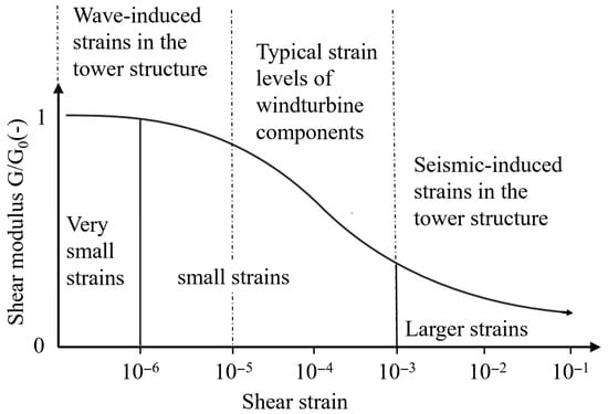
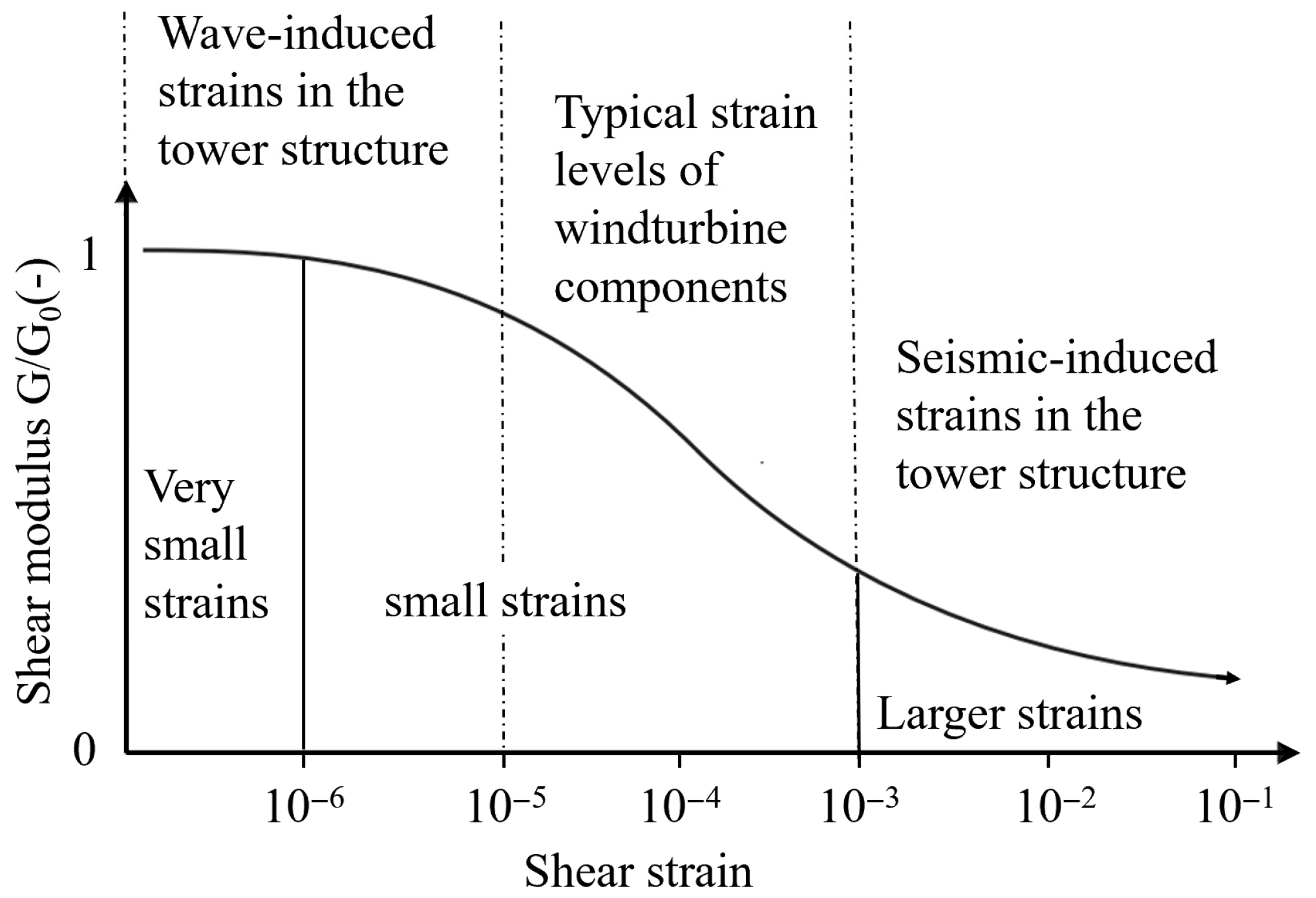
With the advent of high-precision local strain measurement devices (such as LVDTs), it has long been recognized that soils exhibit significant high modulus and non-linear decay characteristics under small-strain conditions (10⁻⁶–10⁻³) [1,2], as illustrated in Figure 1. Traditional theories focusing solely on soil mechanical behavior at conventional strain levels may underestimate the soil stiffness at small strain, leading to low reliability in the prediction of soil deformation around structures.

Figure 1. Variation in shear modulus with shear strain and definition of strain ranges [3,4,5,6].

Selecting an appropriate soil constitutive model is crucial in describing soil characteristics at small strain. Currently, the mainstream constitutive models commonly used in geotechnical engineering include the modified Cam–Clay [7], Mohr–Coulomb, and hardening soil (HS) [8], which was developed based on the Duncan–Chang hyperbolic model [9], etc. Although these models perform well in describing soil deformation under conventional strain conditions, they fail to capture the non-linear degradation mechanism of the shear modulus during the transition from very small strain ($\epsilon <{10}^{-6}$) to conventional strain.

To overcome this shortcoming, Benz et al. developed the hardening soil model with small-strain stiffness (HSS) based on the HS model by incorporating a small-strain stiffness correction derived from the Hardin–Drnevich relationship and replacing the original Mohr–Coulomb (M-C) failure criterion with the Matsuoka–Nakai failure criterion. Chen et al. [10] and Yin et al. [11] investigated the failure envelopes of suction buckets in clay soil utilizing the HS model, demonstrating its applicability in marine geotechnical engineering problems. Demirci et al. [12] utilized the HSS model to simulate the mechanical behavior of the seabed soil to investigate the serviceability limit state (SLS) bearing capacity of hybrid foundations under multiple environmental loads. Further analysis by Kou et al. [13] regarding the deformation and stiffness of soil surrounding OWT monopiles indicates that, compared to the HS model, the HSS model has significant advantages in the high-precision simulation of the bearing characteristics of OWT foundations. Therefore, for the numerical simulation of marine geotechnical engineering problems with strict deformation control requirements, the HSS model represents a superior choice for reliably describing the mechanical behavior of seabed soils involving both small-strain and conventional strain conditions.

Although the HSS model has been integrated into some commercial geotechnical software such as PLAXIS and Diana, its code is proprietary and requires payment for use. To expand engineering application scenarios, some researchers had focused on the open-source numerical implementation of the HSS model. For instance, Du et al. [14] and Wang et al. [15] implemented the HSS model in ABAQUS via UMAT subroutines; however, these implementations utilized explicit stress integration algorithms, which possess inherent deficiencies regarding computational efficiency [16]. Tang et al. [17] performed a secondary development of the HSS model in FLAC3D, yet their yield surface formulation remained based on the Mohr–Coulomb (M-C) failure criterion of the original HS model rather than the Matsuoka–Nakai (M-N) criterion. Leonardo et al. [18] implemented the HS model with the M-N yield criterion using an implicit integration algorithm and validated it through elemental triaxial tests. However, this work did not incorporate the small-strain stiffness correction characteristic of the HSS model. Consequently, there remains room for improvement in the open-source numerical implementations of the HSS model regarding the algorithmic stability and theoretical completeness.

In the field of marine geotechnics, to address the problem of fluid–structure–seabed interaction (FSSI), Ye et al. [19,20] developed the numerical software FssiCAS (available at https://fssi.ac.cn/download.html (accessed on 1 May 2025)). This software incorporates a comprehensive suite of soil constitutive models, such as Mohr–Coulomb, Drucker–Prager, modified Cam–Clay, PZIII, CSUH [21], bounding surface, and cyclic mobility [22], and has demonstrated specific advantages regarding computational efficiency. The reliability of FssiCAS has been extensively validated across various marine geotechnical problems, including the settlement of port breakwater [23], wave–structure–seabed response [24], wave-induced non-linear dynamics of shallow buried pipelines [25], and seismic dynamics of OWT [26]. Given the advantages of FssiCAS in marine geotechnical simulation and the current absence of the HSS model in its material library, the numerical implementation of the HSS model based on this software holds significant engineering significance.

This study first elucidates the theoretical framework of the HSS model, including its yield function, hardening laws, and flow rule. Subsequently, the numerical implementation of the HSS model is done using the Fortran programming language within the framework of FssiCAS. The reliability of FssiCAS incorporating the HSS model is then validated through a triaxial test and a physical test involving the horizontal loading of the monopile. Finally, taking the four-monopile jacket foundation of an offshore wind turbine (OWT) in Lianjiang County, China, as a representative, the HSS model is adopted to describe the mechanical behaviors of the seabed foundation. The horizontal bearing characteristics of the jacket foundation–seabed system under multi-angle horizontal loading are investigated, and the influence of the horizontal loading angle on the horizontal bearing capacity, jacket displacement, and seabed deformation is quantitatively elucidated.

2. HSS Model Theory

2.1. Theoretical Formulation

The HSS model is derived from the HS model by incorporating a small-strain stiffness correction. Under general triaxial conditions, the shear yield function ($f^s$) of the HS model is

$$f^s={\displaystyle \frac{2q_a}{E_i}}{\displaystyle \frac{q}{q_a-q}}-{\displaystyle \frac{2q}{E_{\mathrm{u}\mathrm{r}}}}-{\gamma }^{ps}$$

(1)

where ${\sigma }_1$, ${\sigma }_2$, and ${\sigma }_3$ are the effective principal stresses; $E_{\mathrm{u}\mathrm{r}}$ is the unloading–reloading modulus; $E_i$ is the initial tangent stiffness; $q_a$ is the asymptotic deviatoric stress of the hyperbolic relationship; and ${\gamma }^{ps}$ is a state parameter related to the accumulated plastic shear strain, which, under triaxial conditions, can be written as ${\gamma }^{ps}={\epsilon }_1^p-{\epsilon }_2^p-{\epsilon }_3^p$ (if ${\epsilon }_v$ = 0 under undrained, then ${\gamma }^{ps}=2{\epsilon }_1^p$).

To address the limitation that a single shear yield surface is unable to describe the compressive yielding under compressive stress paths, Schanz et al. [27] introduced a cap yield surface to construct a double-hardening model. The cap yield function ($f^c$) of the HS model is expressed as

$$f^c={\displaystyle \frac{{\tilde{q}}^2}{{\alpha }^2}}-p^2-p_p^2$$

(2)

where $\tilde{q}$ is a special shear stress measure, defined as $\tilde{q}={\sigma }_1+(\delta -1){\sigma }_2-\delta {\sigma }_3$; $\delta$ is a parameter related to the friction angle, defined as $\delta =(3-\mathrm{s}\mathrm{i}\mathrm{n} \phi )/(3+\mathrm{s}\mathrm{i}\mathrm{n} \phi )$; $\alpha$ is a shape parameter of the cap yield surface; $p$ is the mean effective stress, $p={\sigma }_{ii}/3$; and $p_p$ is the pre-consolidation stress, which controls the expansion and contraction of the cap yield surface.

Since the original HS model adopts the Mohr–Coulomb (M-C) failure criterion, its strength depends solely on the maximum and minimum principal stresses ${\sigma }_1$ and ${\sigma }_3$, neglecting the contribution of the intermediate principal stress ${\sigma }_2$. This limitation leads to rather conservative results under complex stress conditions [28]. Furthermore, the hexagonal shape of the M-C failure criterion in the $\pi$-plane results in non-unique normal vectors at the corners, leading to poor convergence of the HS model in modeling.

To overcome this limitation, Benz et al. [29] replaced the M-C failure criterion with the M-N failure criterion and reformulated the shear yield surface in terms of the mobilized friction angle, deriving the shear yield equation of the HSS model as follows:

$$f^s={\displaystyle \frac{3}{2}}{\displaystyle \frac{q}{E_i}}{\displaystyle \frac{\left(\frac{1-\mathrm{s}\mathrm{i}\mathrm{n} {\phi }_m}{\sin {\phi }_m}\right)}{\left(\frac{1-\mathrm{s}\mathrm{i}\mathrm{n} {\phi }_m}{\sin {\phi }_m}\right)-R_f\left(\frac{1-\mathrm{s}\mathrm{i}\mathrm{n} \phi }{\sin \phi }\right)}}-{\displaystyle \frac{3}{2}}{\displaystyle \frac{q}{E_{\mathrm{u}\mathrm{r}}}}-{\gamma }_s^{ps}$$

(3)

where $q$ is the Roscoe invariant, $q=\sqrt{3J_2}$, $J_2$ is the deviatoric stress tensor, $\phi$ is the material friction angle, and ${\phi }_m$ is the mobilized friction angle. $R_f$ is the failure ratio. According to the M-N failure criterion, ${\phi }_m$ is expressed by the stress invariants under the current stress state:

$${\mathrm{s}\mathrm{i}\mathrm{n}}^2{\phi }_m={\displaystyle \frac{9-(I_1{I}_2/I_3)}{1-(I_1{I}_2/I_3)}}$$

(4)

where $I_1={\sigma }_1+{\sigma }_2+{\sigma }_3$, $I_2={\sigma }_1{\sigma }_2+{\sigma }_2{\sigma }_3+{\sigma }_3{\sigma }_1$, and $I_3={\sigma }_1{\sigma }_2{\sigma }_3$. Furthermore, Equation (4) can be rewritten as a function of $p$, $q$, and the Lode angle $\theta$. The Lode angle is defined by Equation (5):

$$\mathrm{s}\mathrm{i}\mathrm{n}3\theta =-{\displaystyle \frac{3\sqrt{3}}{2}}{\displaystyle \frac{J_3}{J_2^{3/2}}}$$

(5)

Alternatively, ${\phi }_m$ can be written as

$$\sin {\phi }_m={\displaystyle \frac{3q}{6\chi (p+c\mathrm{c}\mathrm{o}\mathrm{t} \phi )+q}}$$

(6)

where $\chi$ is the Lode angle correction function,

$$\chi ={\displaystyle \frac{\sqrt{3}\delta }{2\sqrt{{\delta }^2-\delta +1}}} {\displaystyle \frac{1}{\cos \vartheta }}$$

(7)

$$\left\{\begin{array}{ccccc}\vartheta & =& {\displaystyle \frac{1}{6}}\mathrm{a}\mathrm{r}\mathrm{c}\mathrm{c}\mathrm{o}\mathrm{s}(-1+{\displaystyle \frac{27{\delta }^2(1-\delta {)}^2}{2({\delta }^2-\delta +1)}}{\mathrm{s}\mathrm{i}\mathrm{n}}^2(3\theta ))& \mathrm{f}\mathrm{o}\mathrm{r}& \theta \le 0\\ \vartheta & =& {\displaystyle \frac{\pi }{3}}-{\displaystyle \frac{1}{6}}\mathrm{a}\mathrm{r}\mathrm{c}\mathrm{c}\mathrm{o}\mathrm{s}(-1+{\displaystyle \frac{27{\delta }^2(1-\delta {)}^2}{2({\delta }^2-\delta +1)}}{\mathrm{s}\mathrm{i}\mathrm{n}}^2(3\theta ))& \mathrm{f}\mathrm{o}\mathrm{r}& \theta >0\end{array}\right.$$

(8)

The plastic flow of the shear yield surface adopts a non-associated flow rule:

$$g^s=(p+c\cot \phi ){\displaystyle \frac{6\mathrm{s}\mathrm{i}\mathrm{n} {\psi }_m}{3-\mathrm{s}\mathrm{i}\mathrm{n} {\psi }_m}}$$

(9)

where ${\psi }_m$ is the mobilized dilatancy angle, calculated using the simplified Li method [30]:

$$\mathrm{s}\mathrm{i}\mathrm{n} {\psi }_m=\left\{\begin{array}{c}{\displaystyle \frac{\sin {\phi }_m-\sin {\phi }_{cs}}{1-\sin {\phi }_m\sin {\phi }_{cs}}} \mathrm{f}\mathrm{o}\mathrm{r} \mathrm{s}\mathrm{i}\mathrm{n}{\phi }_m-\mathrm{s}\mathrm{i}\mathrm{n}{\phi }_{cs}\ge 0\\ {\displaystyle \frac{1}{10}}(M{e}^{{\displaystyle \frac{1}{15}}\ln \left({\displaystyle \frac{p_{cs}}{p}}\right)}-\eta ) \mathrm{f}\mathrm{o}\mathrm{r} \mathrm{s}\mathrm{i}\mathrm{n}{\phi }_m-\mathrm{s}\mathrm{i}\mathrm{n}{\phi }_{cs}<0\end{array}\right.$$

(10)

where

$$\sin {\phi }_{cs}={\displaystyle \frac{\sin \phi -\sin \psi }{1-\sin \phi \sin \psi }}$$

(11)

$${\displaystyle \frac{p_{cs}}{p}}={\displaystyle \frac{\eta \mathrm{s}\mathrm{i}\mathrm{n} {\phi }_{cs}(1-\mathrm{s}\mathrm{i}\mathrm{n} {\phi }_m)}{M\mathrm{s}\mathrm{i}\mathrm{n} {\phi }_m(1-\mathrm{s}\mathrm{i}\mathrm{n} {\phi }_{cs})}}$$

(12)

where $\psi$ is the material parameter dilatancy angle, ${\phi }_{cs}$ is the critical state friction angle, $\eta =q/p$ is the stress ratio, $M$ is the critical state stress ratio, and $p_{cs}$ is the equivalent critical state stress ratio.

Simultaneously, to maintain consistency in shape between the shear yield surface and the cap yield surface, the shear stress $\tilde{q}$ in the cap yield function of the HS model is replaced by the Roscoe invariant. Additionally, a correction function $\chi$ is introduced to synchronize the Lode angle dependency of the shear yield surface to the cap yield surface, resulting in the cap yield function of the HSS model:

$$f^c={\displaystyle \frac{q^2}{(\chi \alpha {)}^2}}-p^2-p_p^2$$

(13)

The plastic flow of the cap yield surface adopts an associated flow rule:

$$g^c={\displaystyle \frac{q^2}{(\chi \alpha {)}^2}}-p^2-p_p^2$$

(14)

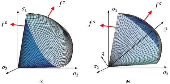
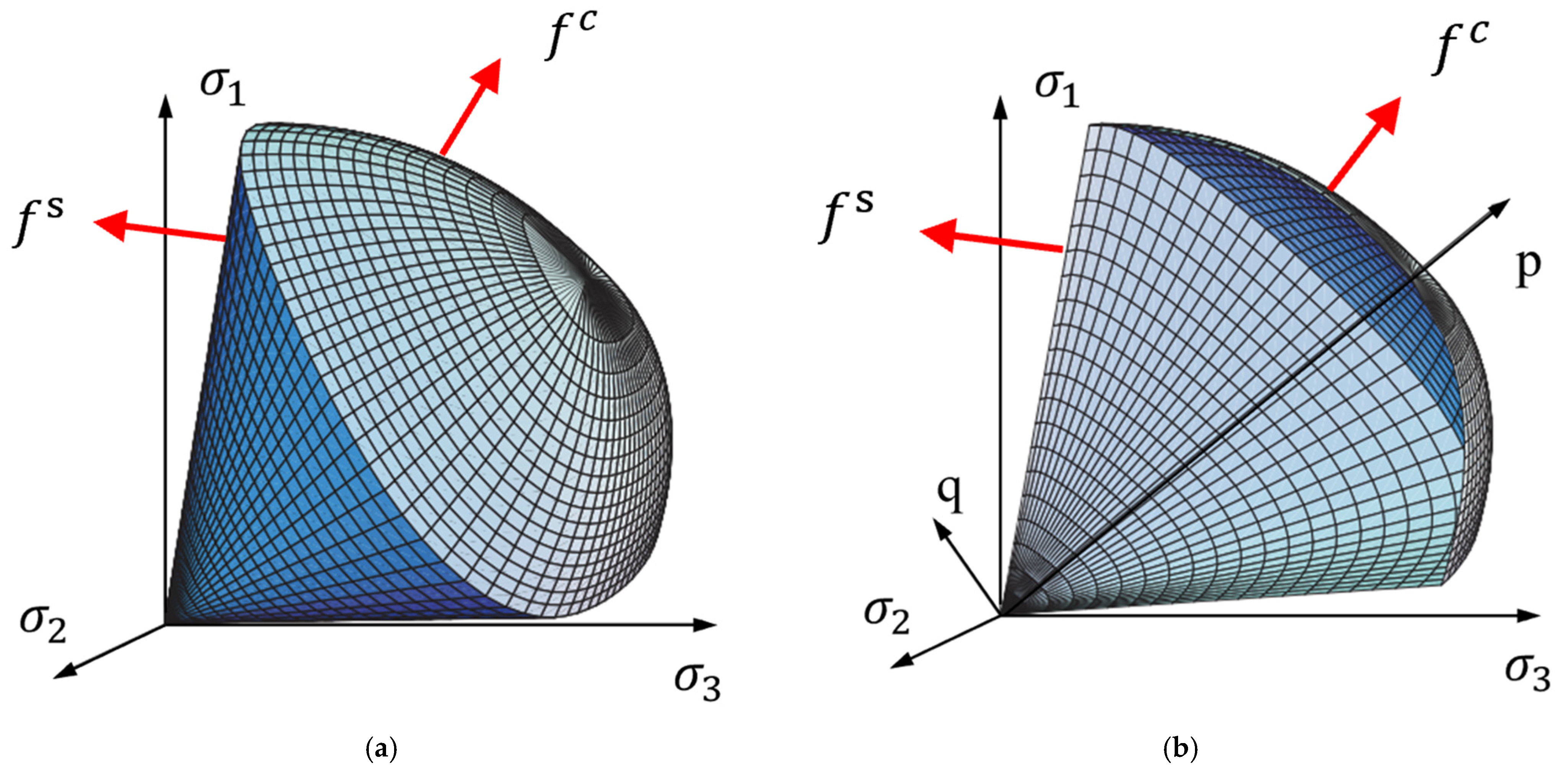
Figure 2 illustrates the yield surfaces of the HSS model in principal stress space and the p-q plane, highlighting the smooth Matsuoka–Nakai criterion and the double-hardening mechanism.

Figure 2. Yield surfaces of the HSS model in the principal stress space. (a) Cap and shear yield surface. (b) p-q slice through the yield surface.

2.2. Small-Strain Stiffness Correction

The modified Hardin–Drnevich model can effectively elucidate the high stiffness and its non-linear degradation exhibited by soils under small-strain conditions:

$${\displaystyle \frac{G}{G_0}}={\left(1+{\displaystyle \frac{3}{7}}\left|{\displaystyle \frac{{\gamma }_{\mathrm{s}}}{{\gamma }_{0.7}}}\right|\right)}^{-1}$$

(15)

where $G_0$ is the initial shear modulus of the soil; ${\gamma }_{0.7}$ is the threshold shear strain at which the shear modulus decays to 0.7$G_0$; and ${\gamma }_{\mathrm{s}}$ is the generalized shear strain.

$$G_0=G_0^{\mathrm{r}\mathrm{e}\mathrm{f}}({\displaystyle \frac{{\sigma }_3+c\mathrm{c}\mathrm{o}\mathrm{t} \phi }{p^{\mathrm{r}\mathrm{e}\mathrm{f}}+c\mathrm{c}\mathrm{o}\mathrm{t} \phi }}{)}^m$$

(16)

where $m$ is the stress-dependency power exponent and $G_0^{\mathrm{r}\mathrm{e}\mathrm{f}}$ is the reference initial shear modulus at small strain.

$${\gamma }_{\mathrm{s}}=\sqrt{{\displaystyle \frac{1}{2}}\left[{\left({\epsilon }_1-{\epsilon }_2\right)}^2+{\left({\epsilon }_2-{\epsilon }_3\right)}^2+{\left({\epsilon }_3-{\epsilon }_1\right)}^2\right]}$$

(17)

Benz et al. [29] further proposed a formula for calculating the shear modulus under small-strain conditions:

$$G=\left\{\begin{array}{c}{G}_0\left({\displaystyle \frac{{\gamma }_{0.7}}{{\gamma }_{0.7}+0.385{\gamma }_{\mathrm{s}}}}\right) {\gamma }_{\mathrm{s}}<{\gamma }_{\mathrm{c}\mathrm{u}\mathrm{t}}\\ {\displaystyle \frac{E_{\mathrm{u}\mathrm{r}}}{2\left(1+\upsilon \right)}} {\gamma }_{\mathrm{s}}\ge {\gamma }_{\mathrm{c}\mathrm{u}\mathrm{t}}\end{array}\right.$$

(18)

where ${\gamma }_{\mathrm{c}\mathrm{u}\mathrm{t}}=7\left[2\right(1+\upsilon )G_0/E_{\mathrm{u}\mathrm{r}}-1]{\gamma }_{0.7}/3$ is the lower limit of stiffness degradation and $E_{\mathrm{u}\mathrm{r}}$ is the unloading and reloading modulus. When the shear strain is less than ${\gamma }_{\mathrm{c}\mathrm{u}\mathrm{t}} \left({\gamma }_{\mathrm{s}}<{\gamma }_{cut}\right)$, the small-strain characteristics of soils should be considered when determining the shear modulus; otherwise $\left({\gamma }_s{\ge \gamma }_{cut}\right)$, it is treated according to the conventional strain state.

2.3. Introduction to Model Parameters

The HSS model needs 16 input parameters. These parameters and the elucidation of their physical meanings are listed in Table 1 [29].

Table 1. Parameters and physical meanings of the HSS model.

Category	Symbol	Physical Meaning	Unit
Stiffness related	$E_{50}^{ref}$	Triaxial secant stiffness	$[\mathrm{k}\mathrm{N}/{\mathrm{m}}^2]$
	$E_{oed}^{ref}$	Oedometric tangent stiffness	$[\mathrm{k}\mathrm{N}/{\mathrm{m}}^2]$
	$E_{ur}^{ref}$	Unloading/reloading stiffness	$[\mathrm{k}\mathrm{N}/{\mathrm{m}}^2]$
	$m$	Power of stress dependency	[-]
	$v_{ur}$	Poisson’s ratio for unloading–reloading	[-]
	$K_0^{nc}$	Coefficient of lateral earth pressure at rest for normal consolidation	[-]
	$p^{ref}$	Reference stress	$[\mathrm{k}\mathrm{N}/{\mathrm{m}}^2]$
Strength related	$c$	Cohesion (effective)	$[\mathrm{k}\mathrm{N}/{\mathrm{m}}^2]$
	$\phi$	Friction angle (effective)	$\left[\begin{array}{c}°\end{array}\right]$
	$\psi$	Dilatancy angle	$\left[\begin{array}{c}°\end{array}\right]$
	$R_f$	Failure ratio	[-]
Small-strain related	$G_0^{ref}$	Reference initial shear modulus at small strains	$[\mathrm{k}\mathrm{N}/{\mathrm{m}}^2]$
	${\gamma }_{0.7}$	$\mathrm{Threshold} \mathrm{shear} \mathrm{strain} \mathrm{at} \mathrm{which} G=0.7G_0$	[-]
Internal parameters	$E_i^{ref}$	Initial secant stiffness	$[\mathrm{k}\mathrm{N}/{\mathrm{m}}^2]$
	$\alpha$	Cap parameter (steepness)	[-]
	$H$	Cap parameter (stiffness ratio)	[-]

3. Numerical Implementation

3.1. Stress Integration Algorithm Framework

The core task of a constitutive model is as follows: given the total stress state and internal state variables (for the HSS model, these are the accumulated plastic shear strain and the pre-consolidation pressure), for a given strain increment at the current incremental step $\left(n\to n+1\right)$, solve for the stress increment and the variation in internal state variables at time $n+1$. In this study, an implicit backward Euler integration algorithm is adopted for the numerical implementation of the HSS model. Plastic stress is corrected by iteratively solving a system of non-linear equations [31,32], wherein the consistency condition is strictly enforced, ensuring high accuracy and good stability. The complete return mapping integration algorithm is divided into two main steps:

(1)

Elastic trial stress calculation: Based on the assumption of purely elastic behavior, the elastic trial stress is calculated as

$${\sigma }^{Trial}={\sigma }^n+{\mathrm{D}}^e:\Delta \epsilon$$

(19)

where ${\sigma }^{Trial}$ is the elastic trial stress, ${\mathrm{D}}^e$ is the tangent elastic stiffness tensor, ${\sigma }_n$ is the stress at the end of the previous incremental step, and $\Delta \epsilon$ is the strain increment of the current incremental step.

(2)

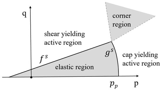
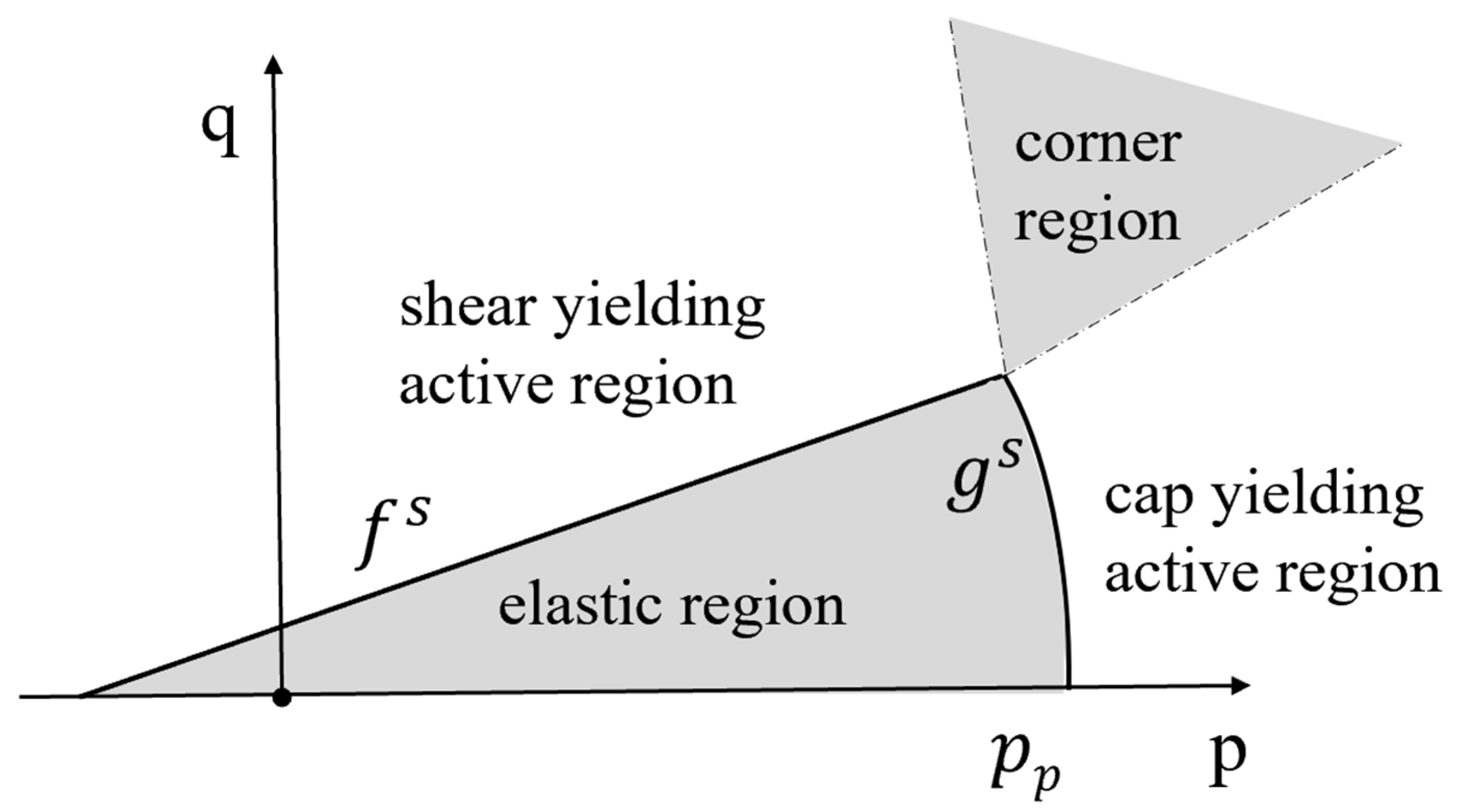
Return mapping plastic correction: After obtaining the elastic trial stress ${\sigma }^{Trial}$, the current stress state and internal state variables are substituted into the yield function for evaluation to determine whether plastic flow occurs in the current incremental step. If $f^s({\sigma }^{Trial},q_{*}^n)\le 0 \mathrm{and} f^c({\sigma }^{Trial},q_{*}^n)\le 0$, the trial stress lies within the elastic domain, and ${\sigma }^{n+1}={\sigma }^{Trial}$ is adopted. If the trial stress lies outside the elastic domain, a return mapping correction is required. Furthermore, as the HSS model features two yield surfaces (shear yield surface $f^s$ and cap yield surface $f^c$), the landing point of the elastic trial stress may be located in three types of inelastic regions (active regions of the shear or cap yield surfaces and the corner region where both yield surfaces are active, as shown in Figure 3). In this study, the two-surface return mapping strategy proposed by Bonnier [33] is adopted to determine the landing point of the plastic trial stress.

Figure 3. Four regions defined by a two-yield-surfaces scheme in the p–q plane.

First, the current state of the yield surfaces is evaluated. If only $f^s>0$ or $f^c>0$, it indicates that the shear (cap) yield surface is currently active, and its consistency condition is solved:

$$f^s\left({\sigma }^{n+1},{\mathrm{q}}_{*}^{n+1}\right)=0 \mathrm{or} f^c\left({\sigma }^{n+1},{\mathrm{q}}_{*}^{n+1}\right)=0$$

(20)

The stress state and state variables are updated via Newton–Raphson iteration. After the single-surface return mapping is completed, the other yield surface must be checked to ensure that the updated stress state remains inside the inactive yield surface. That is, if ${\sigma }^{n+1}$ and ${\mathrm{q}}_{*}^{n+1}$ are obtained through single-surface return mapping based on the shear yield function $f^s$, it is still necessary to further check whether $f^c({\sigma }^{n+1},{\mathrm{q}}^{n+1})\le 0$. If this condition is not satisfied, it indicates that the updated stress point simultaneously exceeds the cap yield surface, and a mixed return mapping is required.

If the trial stress simultaneously satisfies $f^s>0$ and $f^c>0$, indicating that the elastic trial stress lands in the corner region, a mixed return mapping is performed directly to solve the consistency conditions for both yield surfaces:

$$f^s\left({\sigma }^{n+1},{\mathrm{q}}_{*}^{n+1}\right)=0 \mathrm{a}\mathrm{n}\mathrm{d} f^c\left({\sigma }^{n+1},{\mathrm{q}}_{*}^{n+1}\right)=0$$

(21)

Similarly, through Newton–Raphson iteration, the trial stress point is returned to a position that satisfies the dual-surface consistency conditions, thereby obtaining the true stress state and the corresponding state variables [29].

3.2. Consistent Tangent Stiffness Modulus

To ensure the quadratic convergence rate of the integration algorithm under Newton–Raphson (N-R) iteration, it is necessary to use a tangent stiffness matrix that is consistent with the return mapping algorithm during the stress integration process, namely the consistent tangent modulus [34]. In this study, two different consistent tangent moduli, corresponding to single and two yield surfaces, are adopted.

When a single yield surface is active, the consistent tangent modulus can be derived by enforcing the consistency condition on the yield surface. First, by differentiating Equation (20), one obtains

$$d f^{n+1}={\displaystyle \frac{\partial f}{\partial {\sigma }_{ij}}}{|}_{n+1}d{\sigma }_{ij}+{\displaystyle \frac{\partial f}{\partial q_{*}}}{|}_{n+1}d{q}_{*}=n_{ij}^{n+1}d{\sigma }_{ij}+{{\xi }_{*}}^{n+1}d{q}_{*}=0$$

(22)

where ${\sigma }_{ij}$ is the Cauchy stress tensor and $q_{*}$ is the hardening parameter corresponding to this yield surface. $n_{ij}^{n+1}={\displaystyle \frac{\partial f}{\partial {\sigma }_{ij}}}{|}_{n+1},$ ${{\xi }_{*}}^{n+1}={\displaystyle \frac{\partial f}{\partial q_{*}}}{|}_{n+1}$.

The stress update is expressed as

$${\sigma }_{ij}^{n+1}={\sigma }_{ij}^{Trial}-\lambda D_{ijkl}{m}_{kl}^{n+1}$$

(23)

where $m_{kl}^{n+1}$ is the plastic flow direction. From Equation (23), one obtains

$$d{\sigma }_{ij}=D_{ijkl}d{\epsilon }_{kl}-d\lambda D_{ijkl}{m}_{kl}^{n+1}-\lambda D_{ijkl}{\displaystyle \frac{\partial m_{kl}}{\partial {\sigma }_{mn}}}{|}_{n+1}d{\sigma }_{mn}-\lambda D_{ijkl}{\displaystyle \frac{\partial m_{kl}}{\partial q_{*}}}{|}_{n+1}d{q}_{*}$$

(24)

Introducing the hardening modulus,

$$d{q}_{*}=d\lambda h_{*}({\sigma }_{ij},q_{*})$$

(25)

Substituting this into Equation (23), the stress increment is obtained:

$$d{\sigma }_{mn}={\Xi }_{ijmn}{D}_{ijkl}(d{\epsilon }_{kl}-{\Theta }_{kl}d\lambda )$$

(26)

where

$${\Xi }_{ijmn}=({\delta }_{im}{\delta }_{jn}+\lambda D_{ijkl}{\displaystyle \frac{\partial m_{kl}}{\partial {\sigma }_{mn}}}{|}_{n+1}{)}^{-1}$$

(27)

$${\Theta }_{kl}=m_{kl}^{n+1}+\lambda {\displaystyle \frac{\partial m_{kl}}{\partial q_{*}}}{|}_{n+1}{h}_{*}$$

(28)

Substituting Equations (27) and (28) into Equation (22), the consistent algorithmic tangent stiffness $D_{pqmn}^{ep}$ for a single yield surface can be obtained:

$$d{\sigma }_{pq}=D_{pqmn}^{ep}d{\epsilon }_{mn}$$

(29)

where

$$D_{pqmn}^{ep}=\left({\Xi }_{rspq}{D}_{rsmn}\right)-{\displaystyle \frac{\left({\Xi }_{rspq}{D}_{rskl}\right){\Theta }_{kl}{n}_{ij}^{n+1}\left({\Xi }_{rsij}{D}_{rsmn}\right)}{n_{ot}^{n+1}\left({\Xi }_{rsot}{D}_{rspq}\right){\Theta }_{pq}+{\xi }_{*}^{n+1}{h}_{*}}}$$

(30)

When two yield surfaces are active simultaneously, the method proposed by Koiter [35] is used to decompose the plastic strain increment:

$$d{\epsilon }_{ij}^p=d{\lambda }_1{\displaystyle \frac{\partial g_1}{\partial {\sigma }_{ij}}}+d{\lambda }_2{\displaystyle \frac{\partial g_2}{\partial {\sigma }_{ij}}}$$

(31)

where $g_1$ and $g_2$ are the plastic potentials of the two active yield surfaces and $d{\lambda }_1$ and $d{\lambda }_2$ are the corresponding plastic multipliers. In this case, the two active yield surfaces must simultaneously satisfy the consistency conditions:

$$d{f}_1^{n+1}={\displaystyle \frac{\partial f_1}{\partial {\sigma }_{ij}}}{|}_{n+1}d{\sigma }_{ij}+{\displaystyle \frac{\partial f_1}{\partial q_1}}{|}_{n+1}d{q}_1=0$$

(32)

$$d{f}_2^{n+1}={\displaystyle \frac{\partial f_2}{\partial {\sigma }_{ij}}}{|}_{n+1}d{\sigma }_{ij}+{\displaystyle \frac{\partial f_2}{\partial q_2}}{|}_{n+1}d{q}_2=0$$

(33)

The corresponding stress update form is written as

$${\sigma }_{ij}^{n+1}={\sigma }_{ij}^{Trial}-{\lambda }_1 D_{ijkl}{m}_{kl}^{n+1}-{\lambda }_2{D}_{ijkl}{w}_{kl}^{n+1}$$

(34)

Following a derivation process similar to that for a single active yield surface, the consistent algorithmic tangent stiffness tensor for two active yield surfaces can be obtained:

$$D_{pqmn}^{ep}=\left({\Xi }_{rspq}{D}_{rsmn}\right)-\left[{\displaystyle \frac{\left({\Xi }_{rspq}{D}_{rskl}{\Theta }_{kl}^1{n}_{kl}^{n+1}{\Xi }_{rsij}{D}_{rsmn}\right){\mu }_4}{{\mu }_1{\mu }_4-{\mu }_3{\mu }_2}}-{\displaystyle \frac{\left({\Xi }_{rspq}{D}_{rskl}{\Theta }_{kl}^1{\mu }_{kl}^{n+1}{\Xi }_{rsij}{D}_{rsmn}\right){\mu }_2}{{\mu }_1{\mu }_4-{\mu }_3{\mu }_2}}\right]$$

(35)

$$-\left[{\displaystyle \frac{\left({\Xi }_{rspq}{D}_{rskl}{\Theta }_{kl}^2 {\mu }_{kl}^{n+1}{\Xi }_{rsij}{D}_{rsmn}\right){\mu }_1}{{\mu }_1{\mu }_4-{\mu }_3{\mu }_2}}-{\displaystyle \frac{\left({\Xi }_{rspq}{D}_{rskl}{\Theta }_{kl}^2{n}_{kl}^{n+1}{\Xi }_{rsij}{D}_{rsmn}\right){\mu }_3}{{\mu }_1{\mu }_4-{\mu }_3{\mu }_2}}\right]$$

where

$$\left\{\begin{array}{c}{\mu }_1=n_{ij}^{n+1}{\Xi }_{ijmn}{D}_{ijkl}{\Theta }_{kl}^1-{\xi }_1{h}_1\\ {\mu }_2=n_{ij}^{n+1}{\Xi }_{ijmn}{D}_{ijkl}{\Theta }_{kl}^2\\ {\mu }_3=u_{ij}^{n+1}{\Xi }_{ijmn}{D}_{ijkl}{\Theta }_{kl}^1\\ {\mu }_4=u_{ij}^{n+1}{\Xi }_{ijmn}{D}_{ijkl}{\Theta }_{kl}^2-{\xi }_2{h}_2\end{array}\right.\begin{array}{c}{\xi }_1={\left.{\displaystyle \frac{\partial f_1}{\partial q_1}}\right|}_{n+1},{\xi }_2={\left.{\displaystyle \frac{\partial f_2}{\partial q_2}}\right|}_{n+1},h_1={\left.{\displaystyle \frac{d{q}_1}{d{\lambda }_1}}\right|}_{n+1},h_2={\left.{\displaystyle \frac{d{q}_2}{d{\lambda }_2}}\right|}_{n+1}\\ \end{array}$$

(36)

4. Model Validation

4.1. Triaxial Compression Elemental Test

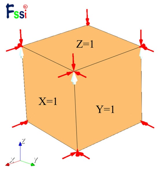
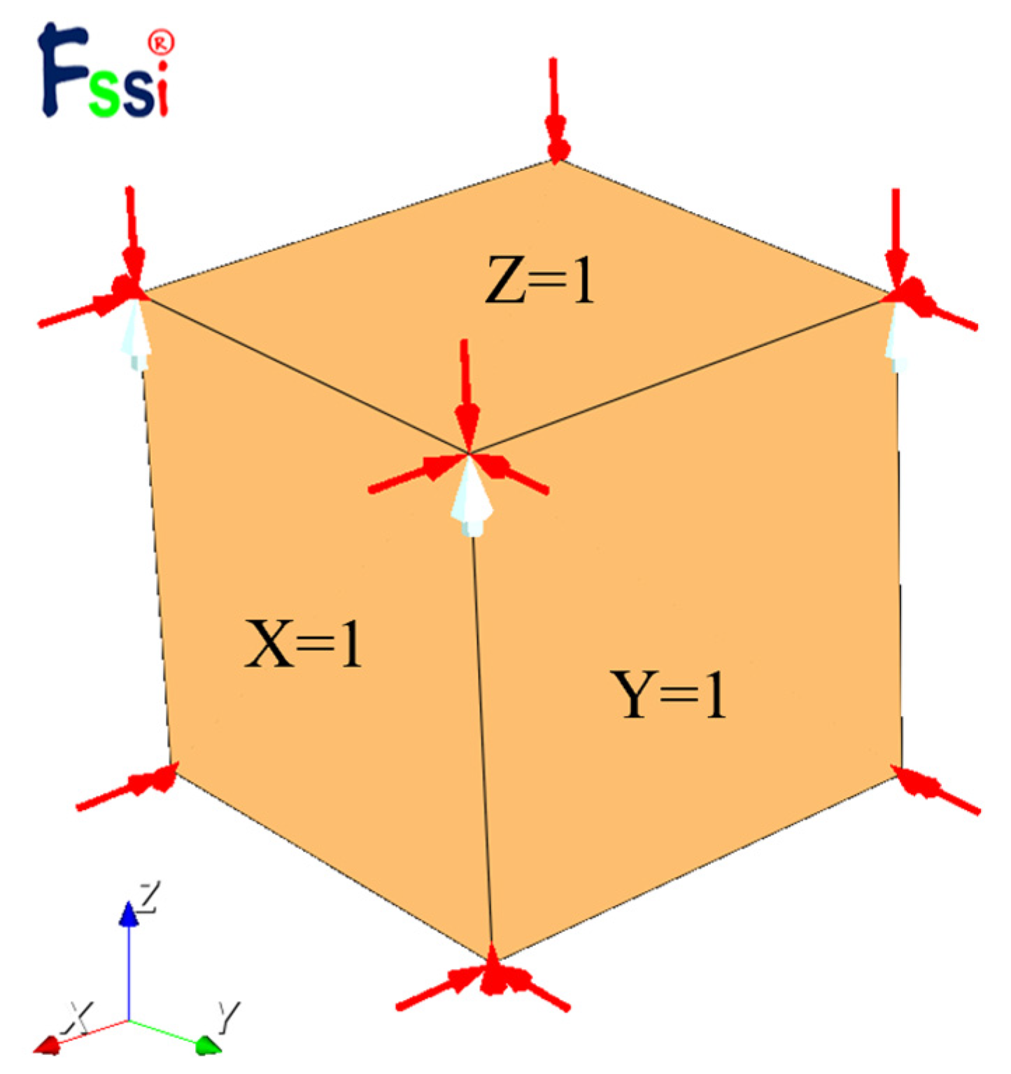
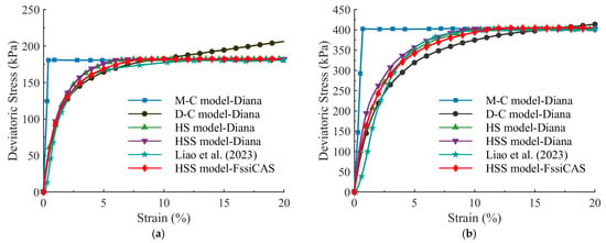
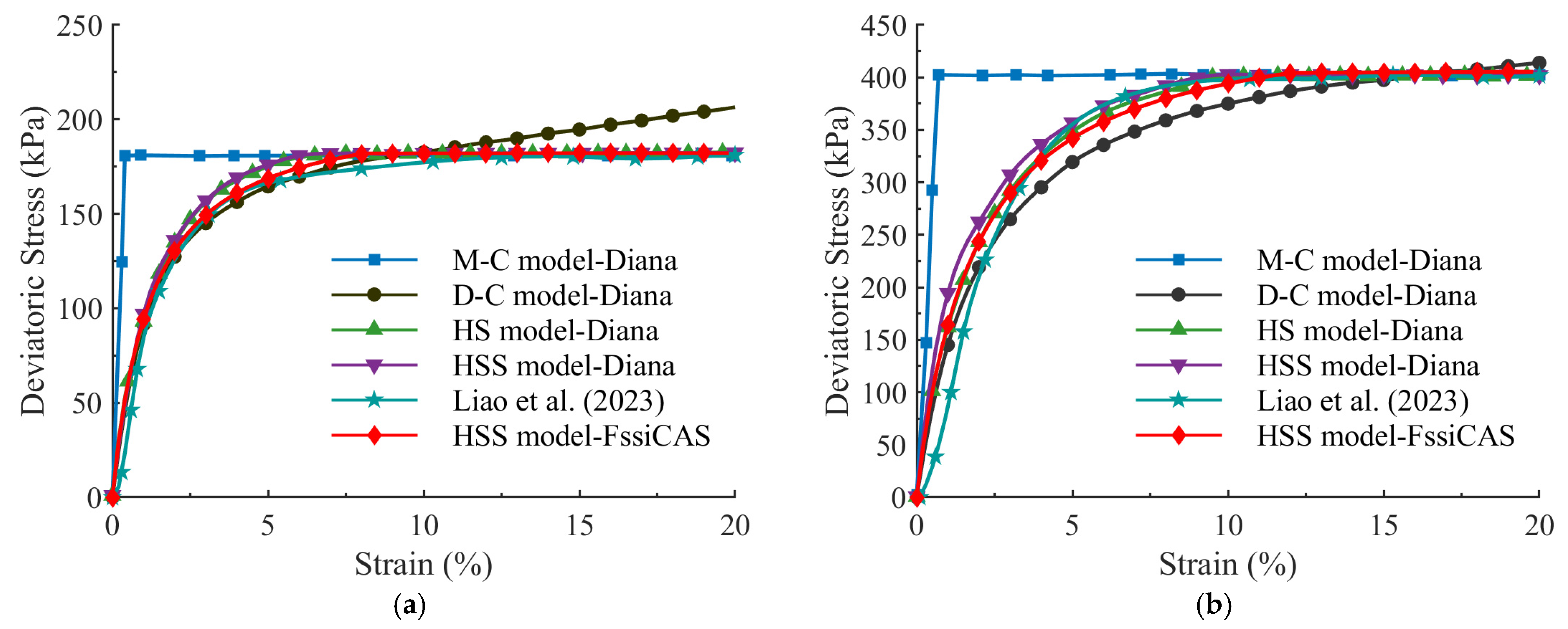
The reliability of the developed HSS model in the framework of FssiCAS is validated using a soil elemental triaxial compression test reproducing the consolidated undrained (CU) tests on loess soil from Liao et al. [36], as shown in Figure 4. This method has been widely applied to verify the reliability of constitutive models [37,38,39]. The boundary conditions are set as follows: normal displacement constraints are applied to the three planes X = 0, Y = 0 and Z = 0, while a confining pressure of 100 kPa or 300 kPa is applied to the remaining three free surfaces (X = 1, Y = 1 and Z = 1), neglecting the influence of the model’s minor self-weight. The loading method adopts the way of displacement control, applying vertical displacement on the plane Z = 1 along the negative Z-axis direction at a strain loading rate of 0.2% per second until the element reaches 20% axial strain. The soil parameters are consistent with those in Liao et al. [36], as shown in Table 2. The stress–strain relationship predicted by FssiCAS incorporating the HSS model is compared with the test results from Liao et al. [36] as well as the numerical results using other models in the commercial Diana, as shown in Figure 5. The comparison results indicate that, compared to the HSS model in Diana and other commonly used soil models, the prediction of HSS–FssiCAS exhibits a higher degree of agreement with the experimental data.

Figure 4. Schematic diagram of a single-element triaxial compression test for the numerical verification (red arrows indicate the boundary conditions of confining pressure; white arrows indicate the applied axial displacement).

Table 2. Parameters of the HSS model in the validation case (unit of modulus, pressure and c is kPa; unit of $\phi$ and $\psi$ is $°$).

$E_{50}^{ref}$	$E_{oed}^{ref}$	$E_{ur}^{ref}$	$m$	$v_{ur}$	$K_0^{nc}$	$p^{ref}$	$c$
9990	8330	49,960	0.5	0.2	0.644	100	24.65
$\phi$	$\psi$	$R_f$	$G_0^{ref}$	${\gamma }_{0.7}$	$E_i^{ref}$	$\alpha$	$H$
20.84	0	0.88	149,880	3 × 10−4	19,563	1.05	33,857

Note: Unit of modulus, pressure and c is kPa; unit of $\phi$ and $\psi$ is $°.$

Figure 5. Comparison of deviatoric stress–strain curves between numerical results and test data (Liao et al., 2023 [36]) (M-C: Mohr–Coulomb model, D-C: Duncan–Chang model, and HS: hardening soil model). (a) ${\sigma }_3=100 \mathrm{k}\mathrm{P}\mathrm{a}$. (b) ${\sigma }_3=300 \mathrm{k}\mathrm{P}\mathrm{a}$.

4.2. Physical Model Test Validation

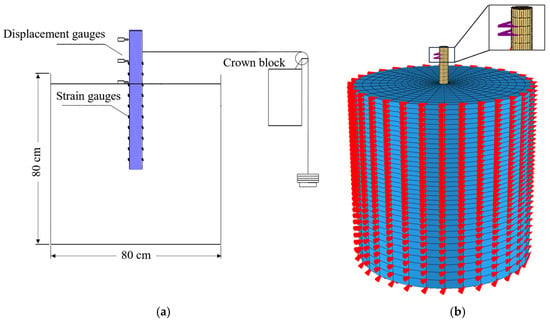
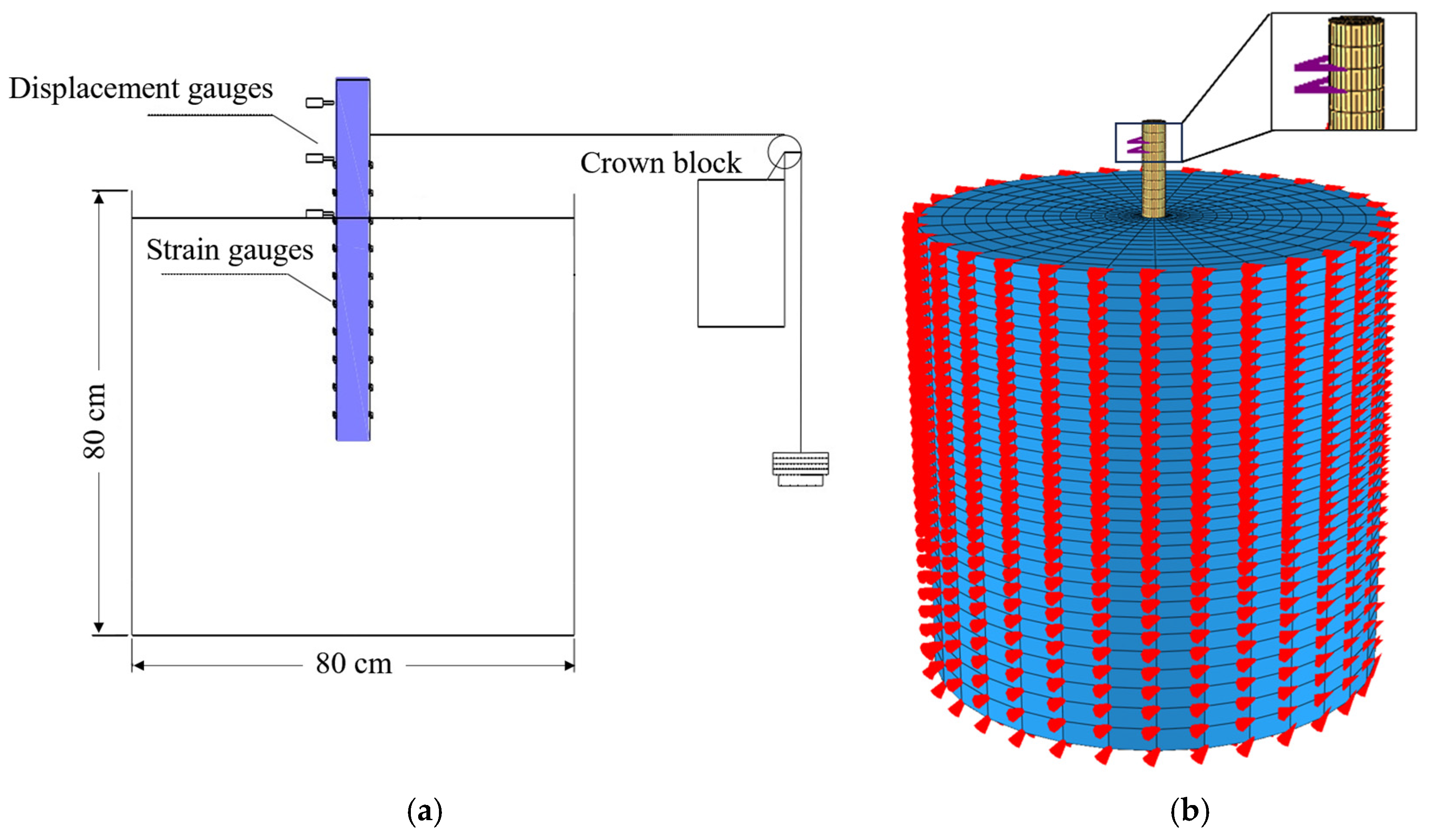
To validate the reliability of the HSS model implemented in FssiCAS under complex soil–structure interaction conditions, the horizontal bearing capacity test of a single pile conducted by Chen et al. [40] is selected as the benchmark. The test configuration and numerical model are shown in Figure 6.

Figure 6. Verification against a horizontal bearing test of the monopile. (a) Physical experimental setup. (b) Numerical model.

The physical model has a pile length of 70 cm, an embedment depth of 50 cm, an outer diameter D = 6 cm, an inner diameter d = 5.5 cm, and a wall thickness t = 5 mm. In the numerical model in FssiCAS, based on the principles of equivalent flexural stiffness and equivalent mass, the pipe pile is simplified to an equivalent solid pile with a diameter of 5 cm and a density of ${\rho }_2=616$ kg/m³. The finite element mesh for the entire model consists of approximately 15,000 hexahedral elements. To eliminate boundary effect, the radius of the foundation soil around the pile is set to 10 times the pile diameter, and its height is set to twice the embedment depth. The boundary conditions are set such that horizontal displacement is fixed on the lateral sides of the foundation and displacement in all directions is fixed at the bottom. Regarding the pile–soil interface, a shared-node approach is employed to simulate the connection between the pile and the surrounding soil, which maintains high reliability and accuracy for the load levels considered in this study, where large-scale sliding is not involved [41]. The loading scheme in the numerical modeling is consistent with that of Chen et al. [40]; corresponding to the experimental setup, a lateral horizontal load from 0 to 400 N is applied incrementally at the height of 15 cm above the mudline on the monopile. The numerical model is shown in Figure 6b. A linear elastic constitutive model is applied to the jacket structure. The soil parameters are calibrated based on the tests by Chen et al. [40] and relevant empirical formulas [42], as listed in Table 3.

Table 3. Parameters of HSS model for the soil in Chen et al. (2018) [40].

$E_{50}^{ref}$	$E_{oed}^{ref}$	$E_{ur}^{ref}$	$m$	$v_{ur}$	$K_0^{nc}$	$p^{ref}$	$c$
35,000	35,000	105,000	0.5	0.21	0.56	100	8.2
$\phi$	$\psi$	$R_f$	$G_0^{ref}$	${\gamma }_{0.7}$	$E_i^{ref}$	$\alpha$	$H$
26	0	0.9	2 × 105	3.3 × 10−4	67,878	1.47	90,643

Note: Unit of modulus, pressure and c is kPa; unit of $\phi$ and $\psi$ is $°.$

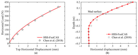
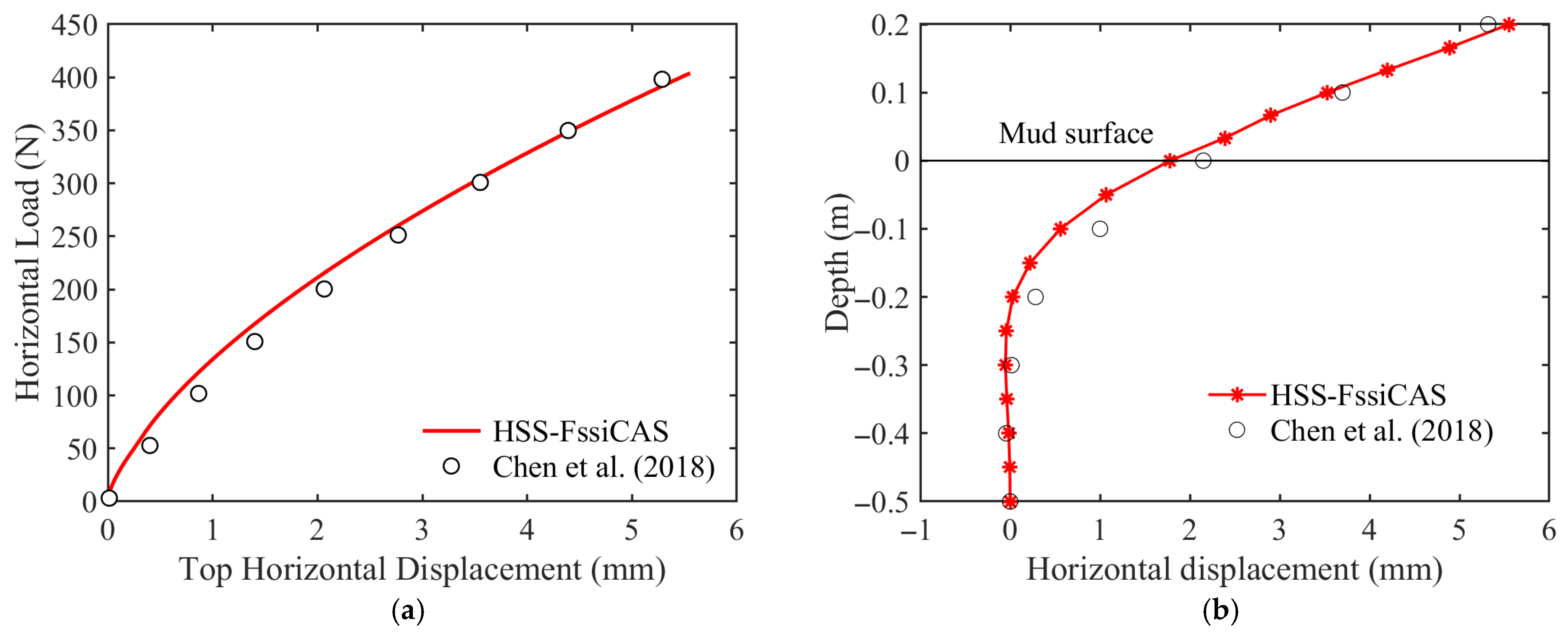
Figure 7a presents the horizontal load–displacement curve at the pile head (20 cm above the mudline). The numerical results by FssiCAS incorporating the HSS model show good agreement with the experimental results (Chen et al., 2018 [40]), demonstrating a high reliability for the hybrid of FssiCAS and the HSS model.

Figure 7. Comparison between the predicted and measured results from Chen et al. (2018) [40] involving a monopile horizontal bearing test. (a) Load–displacement at the pile head. (b) Lateral deformation at a load of 400 N.

Figure 7b illustrates the horizontal displacement of the monopile under a horizontal load of 400 N. Under horizontal loading, the pile displacement is mainly concentrated in the segment below the mudline of 0.2 m. At the deeper buried depth, the lateral horizontal displacement decays rapidly, becoming nearly zero at the pile base. Significant bending deformation occurs along the pile segment between the buried depth of 0.2 m and 0.1 m. For the pile segment from the buried depth of 0 to 0.1 m and the segment above the mudline, the curvature slope remains essentially consistent, indicating that the pile exhibits the typical deformation behavior of flexible piles. The computational results by HSS–FssiCAS reliably reproduce the experimental data, fully demonstrating the high reliability and robustness of the HSS model implemented within the framework of FssiCAS in addressing pile–soil interaction problems.

5. Horizontal Bearing Characteristics of Offshore Jacket Foundation

With the global transition of energy structures and reliance on its long coastline and abundant offshore wind resources, China’s offshore wind power industry has entered a period of large-scale and rapid development. The jacket foundation, due to its high stiffness and light weight, has become the mainstream supporting structure for future deep-water wind turbines. However, as a key component supporting the entire turbine and transferring complex environmental loads, the jacket foundation is prone to lateral cumulative displacement under the long-term action of multi-directional horizontal loads induced by wind, waves, and currents. Zhu et al. [43] investigated the mechanical behavior of jacket pile foundations under orthogonal and diagonal loading directions through physical experiments; however, they did not perform a quantitative analysis of the bearing capacity characteristics. Zhu et al. [44] analyzed the influence of different loading angles on the bearing capacity of jacket foundations, but due to the limitations of the simplified soil constitutive model employed, they failed to analyze the refined deformation characteristics of the foundation soil. Meanwhile, relevant standards have imposed strict requirements on the deformation behavior of jacket pile foundations; for example, DNVGL-2018 [45] recommends that the inclination angle of fixed wind turbines should not exceed 0.5°, while NB/T10105-2018 [46] sets a lateral rotation limit of 0.17° for large-scale wind turbines with a tower height exceeding 100 m. Applying the HSS–FssiCAS model enables a refined analysis of the lateral deformation of jacket foundations and the deformation of the surrounding seabed foundation, which holds significant engineering importance for optimizing the design of the jacket, evaluating the long-term service performance of entire structures, as well as meeting the stringent requirements for the lateral displacement during operation and service.

5.1. Geometric Model

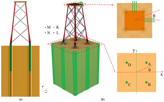
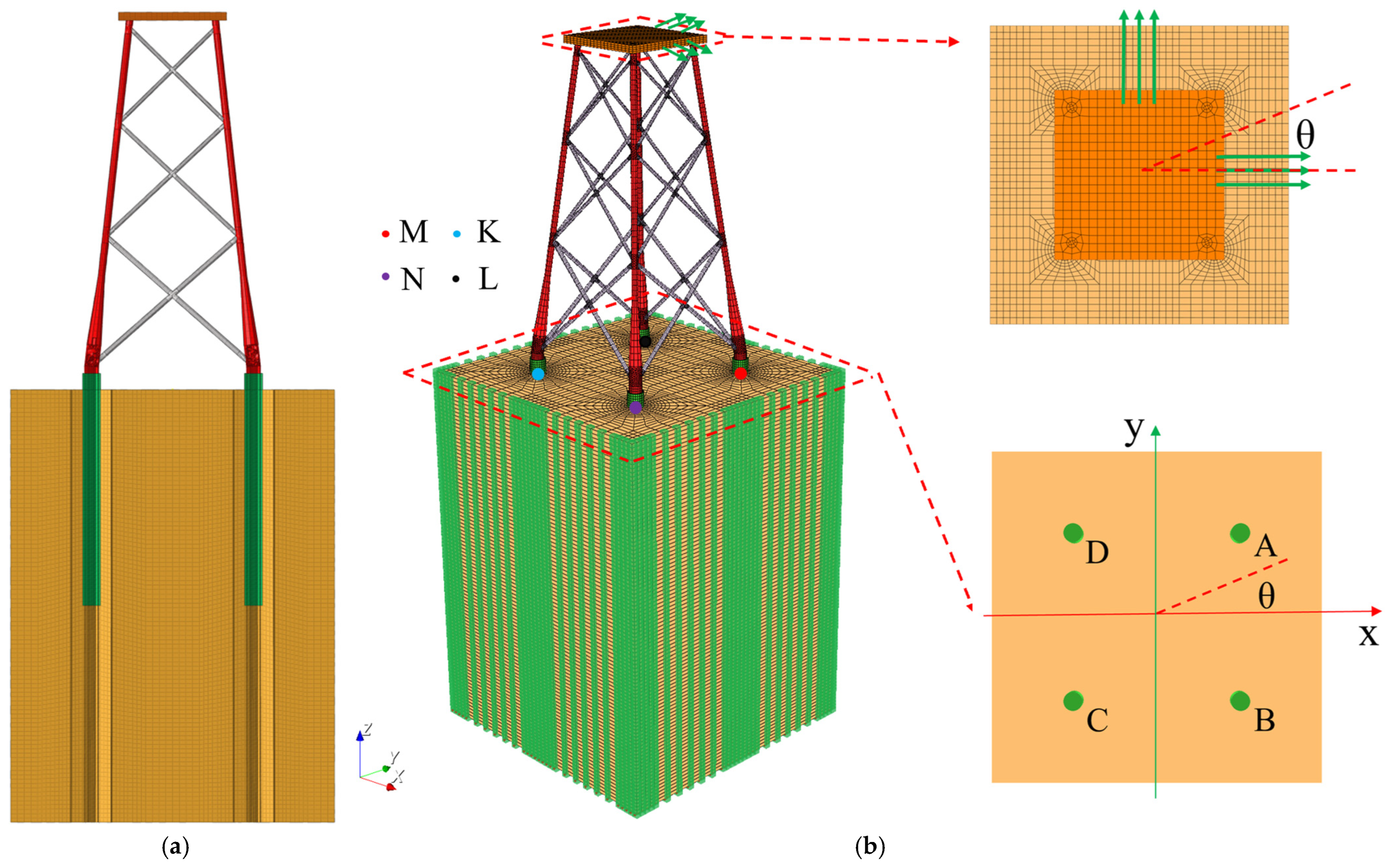
In this paper, a numerical model of the interaction between a jacket foundation and the seabed is established with reference to a four-monopile jacket foundation for an offshore wind turbine in Lianjiang County, China, as shown in Figure 8a. The jacket foundation consists of four hollow single piles with a length L = 40 m, wall thickness t = 0.1 m, and outer diameter D = 3.4 m, combined with a 70 m high jacket structure. Considering the difficulty of meshing all thin-walled steel pipe structures in the global model and following the principles of equivalent flexural stiffness and equivalent mass [47], the hollow thin-walled sections of the jacket and single piles are simplified into solid sections in the numerical modeling. The material parameters of each component after equivalence are detailed in Table 4.

Figure 8. 3D finite element model for the jacket foundation–monopile–seabed system in FssiCAS (A–D denote the IDs of the piles. M, N, K, and L denote the IDs of the four monitoring points). (a) Local cross-sectional mesh. (b) Global model setup.

Table 4. Equivalent parameters of the jacket structure.

Jacket Structure	Elastic Modulus (Equivalent)/GPa	Density (Equivalent)/kg/m3	Poisson’s Ratio/μ
Platform	2 × 1011	7850	0.3
Jacket leg	5.7 × 1010	1059.56	0.3
Jacket brace	7 × 1010	1801.12	0.3
pile	4.4 × 1010	901.95	0.3

The computational domain for the seabed foundation is taken as 60 m (L) × 60 m (W) × 100 m (H), employing hexahedral elements with approximately 190,000 elements. The piles and the jacket structure utilize a mix of tetrahedral and hexahedral elements, with approximately 70,000 elements. Periodic boundary conditions are applied to the four lateral sides of the seabed foundation to fully eliminate the boundary effect [48], while displacement constraints in X, Y, and Z are applied to the bottom of the seabed foundation. The 3D finite element model of the jacket foundation–monopile–seabed system, analyzed using FssiCAS, is shown in Figure 8.

To explore the horizontal bearing characteristics of the jacket foundation under multi-angle horizontal loads in a complex marine environment and comprehensively considering the symmetry of the jacket foundation itself, computational efficiency, and the effect of different load magnitudes, a horizontal load with a final magnitude of 28.8 MN is applied to the jacket platform. The load is applied at a uniform loading rate of 288 kN/s, with deviation angles relative to the positive X-axis of $\theta$= 0°, 15°, 30° and 45°, respectively. Simultaneously, four typical positions at the head center of the monopile axis, M (15, 15, 0), N (15, −15, 0), K (−15, −15, 0), and L (−15, 15, 0), are set to monitor the lateral displacement response of the four monopiles.

Given the significant status of the Yangjiang sea area in China’s offshore wind power engineering, this study selects the typical seabed soil from the Yangjiang sea area as the foundation. The HSS constitutive parameters, calibrated by Yuan et al. [49] based on the seabed soil sampled from the site of the Guangdong Yangjiang Shapa Phase III and V offshore wind farms, are adopted as input parameters and listed in Table 5.

Table 5. Parameters of the HSS model for the seabed foundation.

$E_{50}^{ref}$	$E_{oed}^{ref}$	$E_{ur}^{ref}$	$m$	$v_{ur}$	$K_0^{nc}$	$p^{ref}$	$c$
10,400	10,400	62,800	0.5	0.2	0.4	100	8.2
$\phi$	$\psi$	$R_f$	$G_0^{ref}$	${\gamma }_{0.7}$	$E_i^{ref}$	$\alpha$	$H$
36.7	6.7	0.68	149,880	3 × 10−4	21,000	1.64	25,750

Note: Unit of modulus, pressure and c is kPa; unit of $\phi$ and $\psi$ is $°.$

First, the initial state after the construction completion of the jacket foundation is determined. The corresponding displacement and strain fields are then reset to zero, while the initial stress field is taken as the initial condition for subsequent computation. On this basis, horizontal loads are applied, and an analysis of the bearing characteristics of the jacket foundation–seabed system is carried out. It should be noted that fluid–structure interaction is not involved in this study; thus, pore water pressure is neglected, making the total stress equivalently equal to the effective stress.

5.2. Results and Analysis

5.2.1. Horizontal Displacement

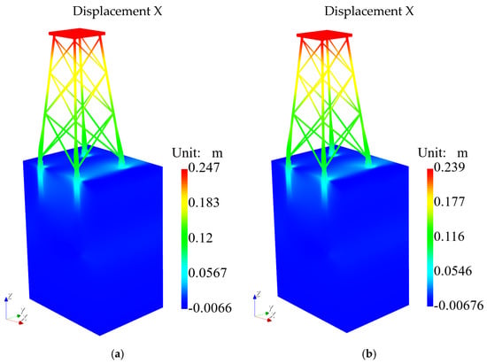
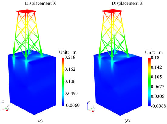
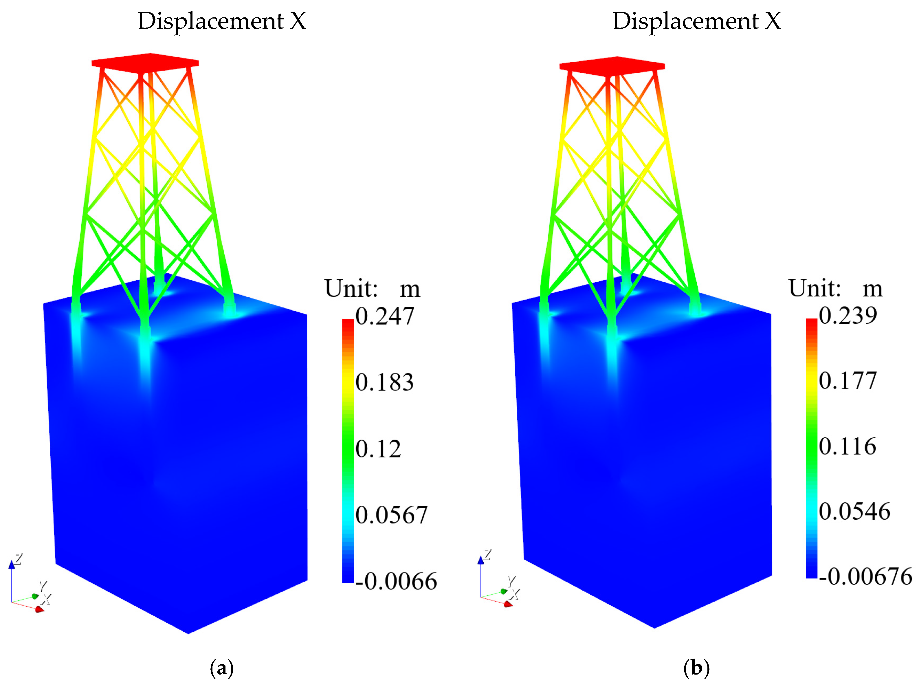
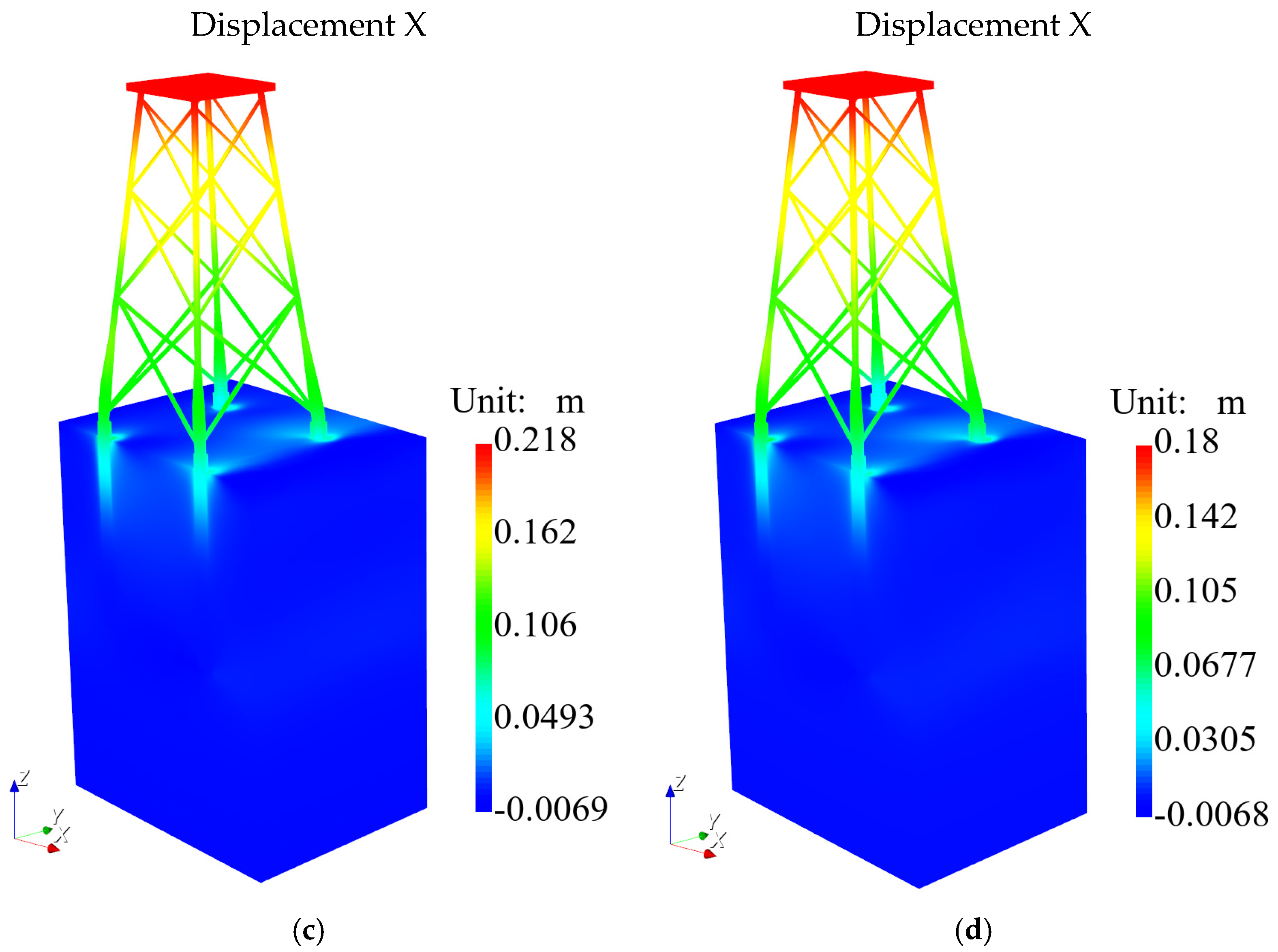
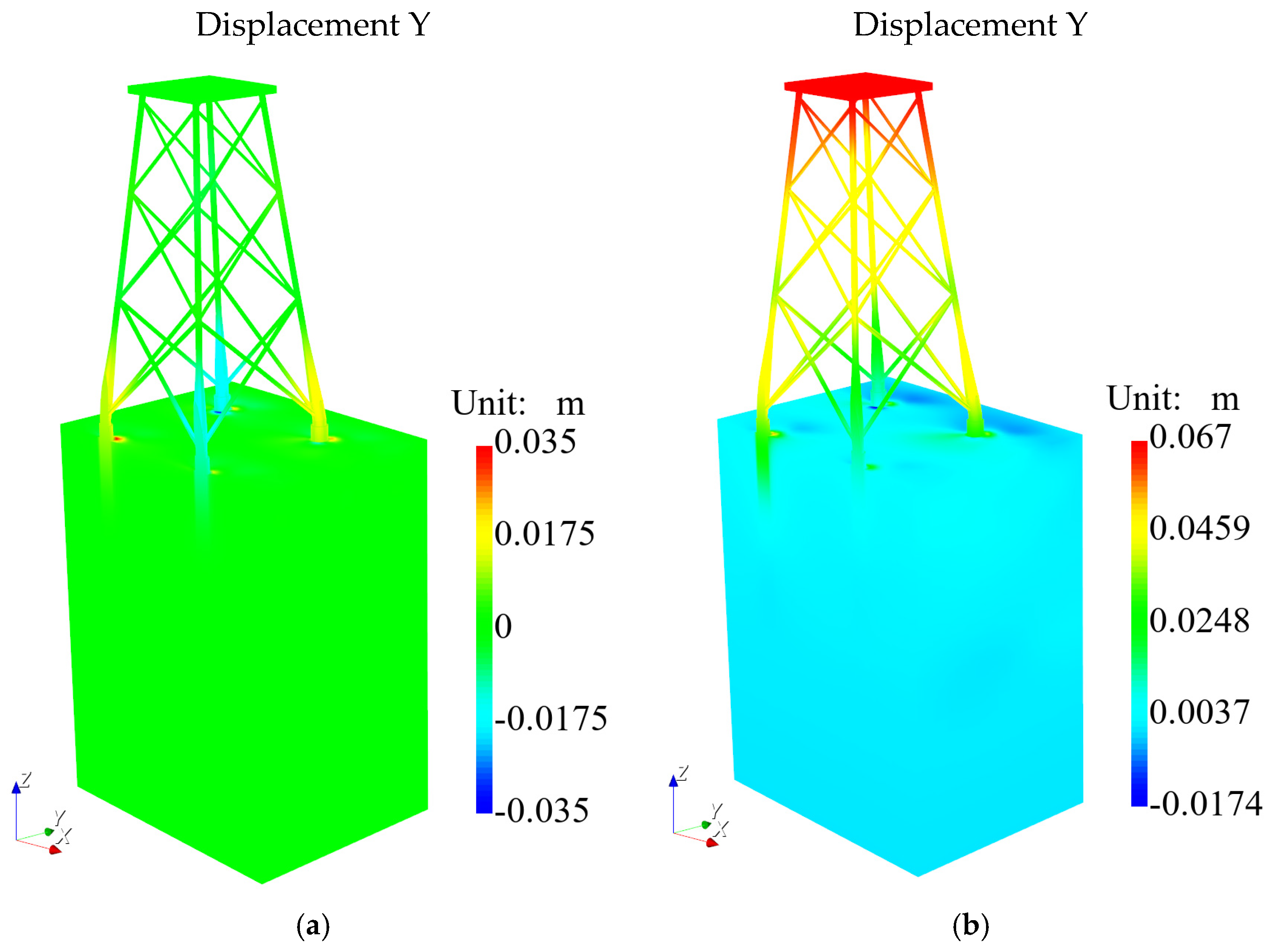
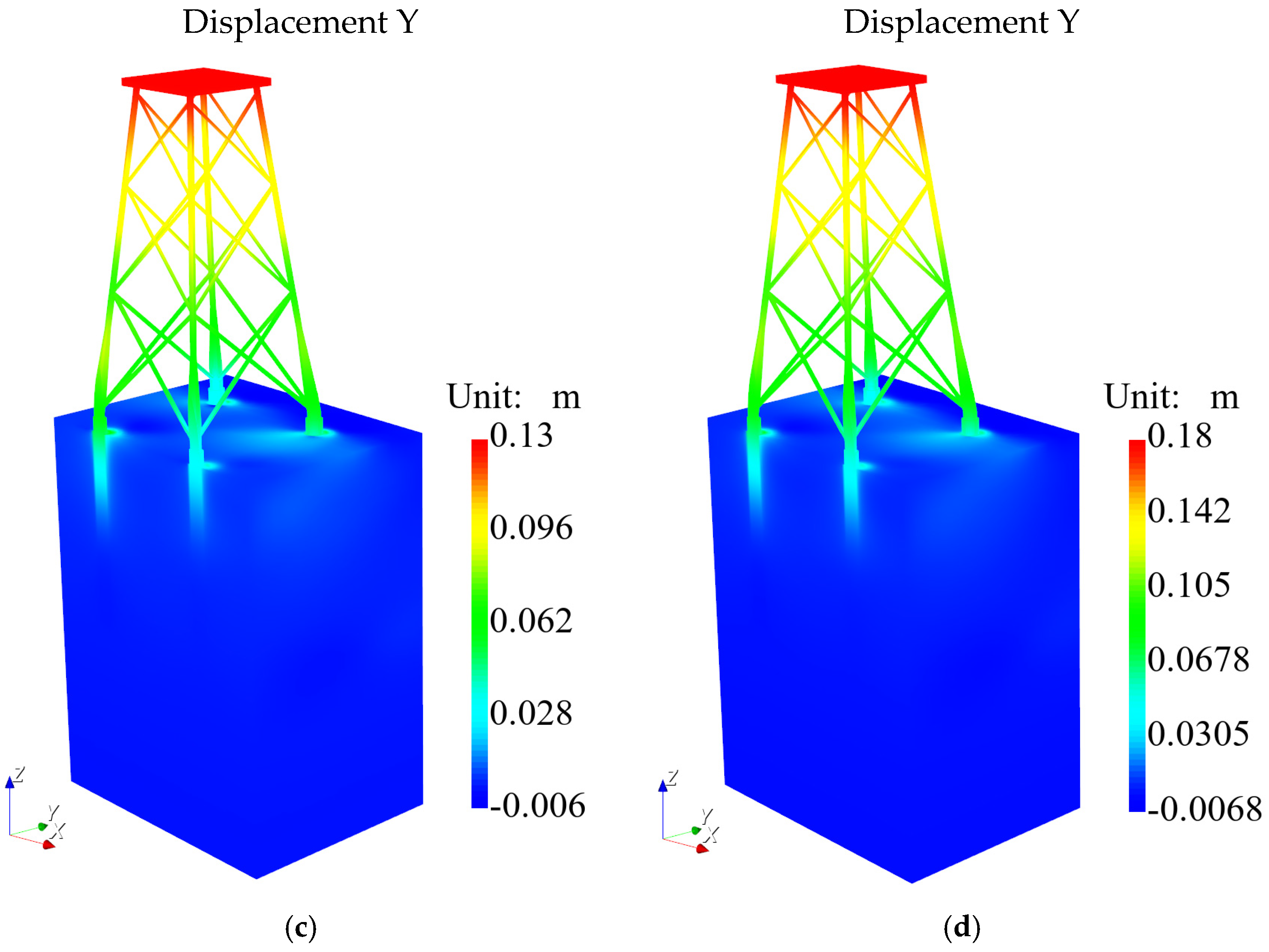
Figure 9 and Figure 10 illustrate the displacement distributions of the jacket and seabed in the X and Y directions at the final time (with an applied force of F = 28.8 MN) under different loading directions. In the case of $\theta$ = 0°, where the horizontal load is entirely parallel to the X-axis, the maximum displacement at the jacket top reaches 0.247 m, with the region of large deformation mainly concentrated in the upper part of the jacket. Near the mudline, the displacement in the X-direction becomes significantly smaller due to the confining resistance from the surrounding soil. As the loading angle $\theta$ increases, the load component in the X-direction, $F_{\mathrm{x}}=F\mathrm{c}\mathrm{o}\mathrm{s}\theta$, decreases accordingly, leading to a gradually decreasing trend in the maximum displacement at the jacket top. It decreases from 0.247 m when $\theta$ = 0° to 0.180 m when $\theta$ = 45°, a reduction of approximately 27%. In the Y-direction, when $\theta$ = 0°, the load component is zero; however, the contour plot reveals a minor displacement of approximately 0.035 m in the soil around the monopiles, exhibiting a distribution symmetric about the X-axis. This is because, as the jacket displaces in the X-direction, the soil around the monopiles is symmetrically compressed in the positive and negative Y-directions, producing minor lateral symmetric deformation. As the angle $\theta$ increases, the load component in the Y-direction, $F_{\mathrm{y}}=F\mathrm{s}\mathrm{i}\mathrm{n}\theta$, gradually increases, and the compressive deformation of the foundation soil in the Y-direction increases significantly. At $\theta$ = 45°, $F_{\mathrm{x}}$ = $F_{\mathrm{y}}$. Due to the diagonal symmetry characteristics of the four-monopile jacket foundation, the values and patterns of the displacement contours in the X and Y directions are identical.

Figure 9. X-displacement distribution of the jacket foundation and seabed at F = 28.8 MN. (a) $\theta$ = 0°, (b) $\theta$ = 15°, (c) $\theta$ =30°, (d) $\theta$ = 45°.

Figure 10. Y-displacement distribution of the jacket foundation and seabed at F = 28.8 MN. (a) $\theta$ = 0°, (b) $\theta$ = 15°, (c) $\theta$ =30°, (d) $\theta$ = 45°.

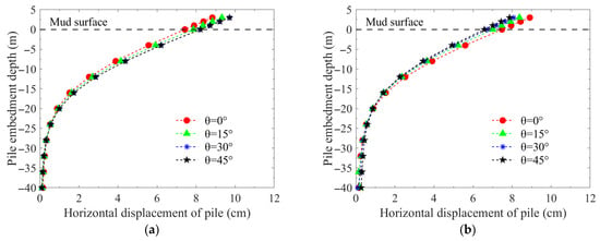
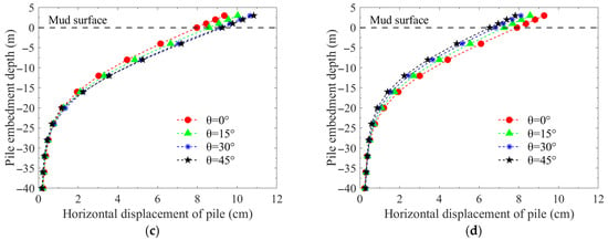
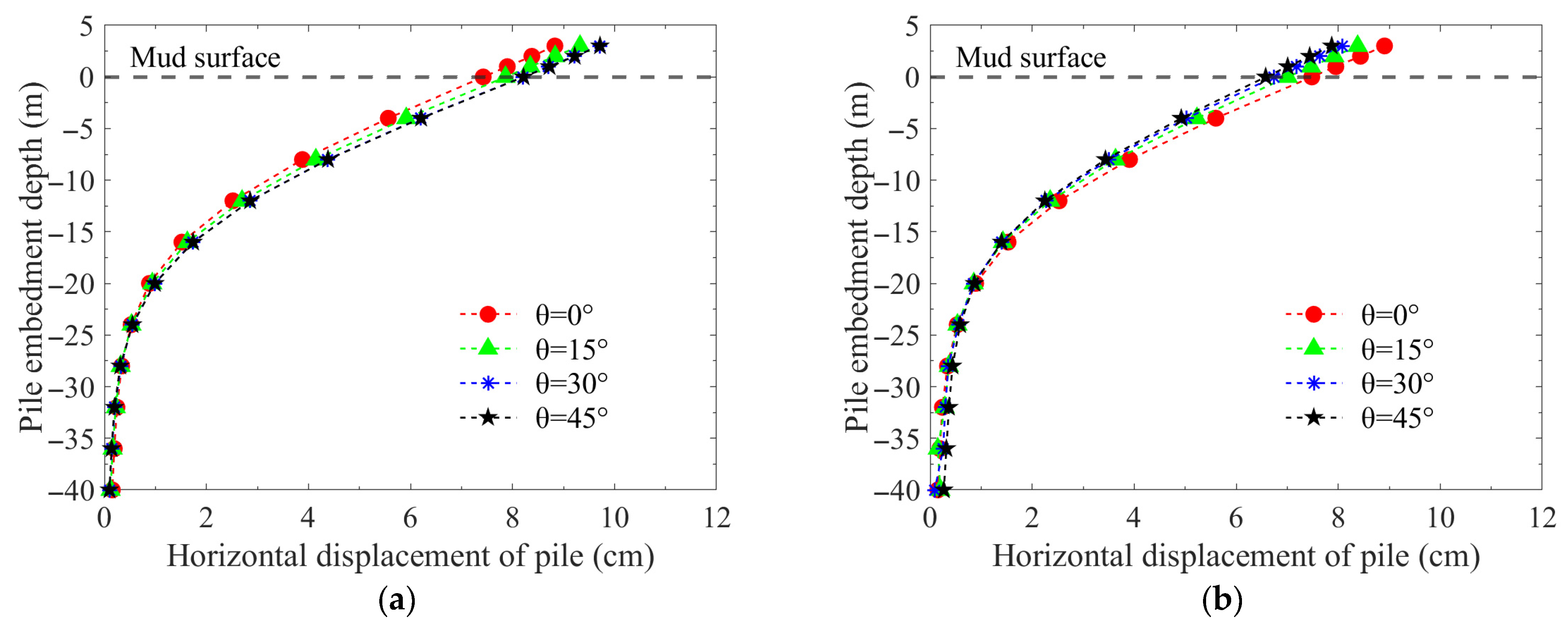
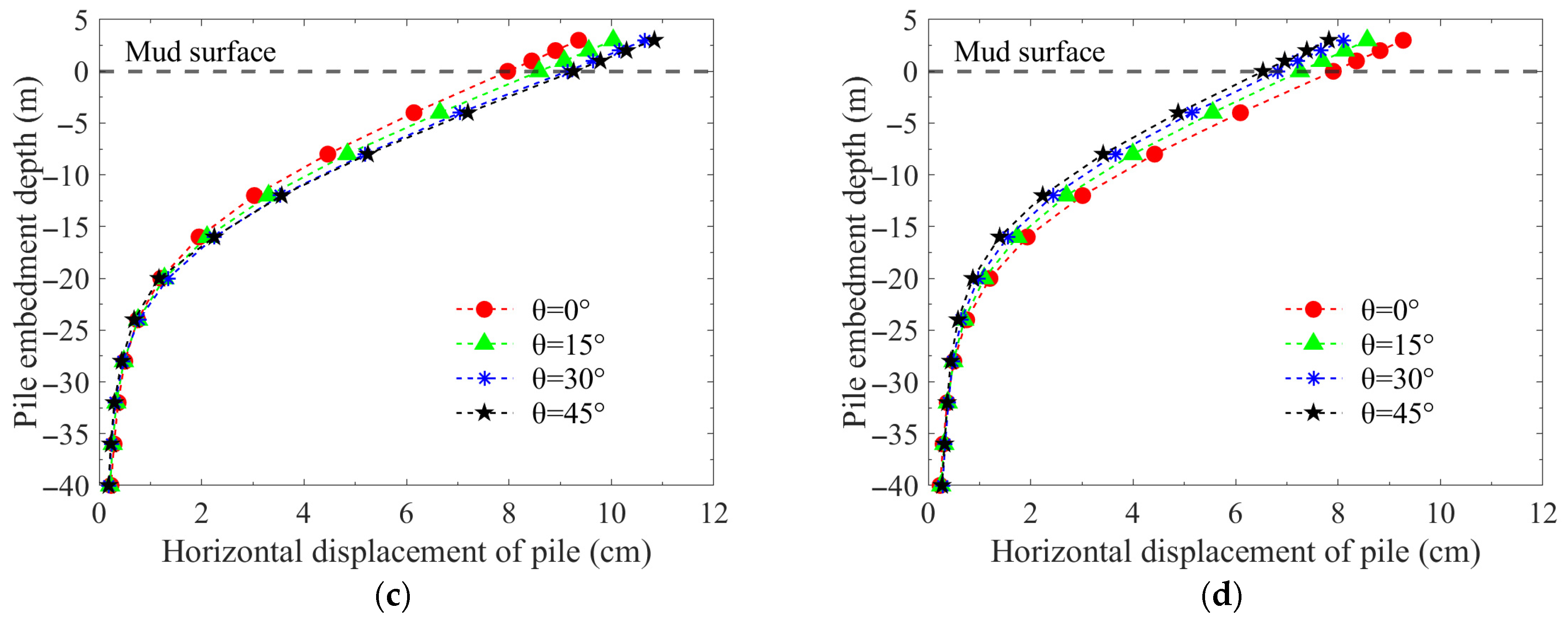
The distribution of horizontal displacement with embedment depth for each individual pile under different horizontal loading angles is analyzed below to quantitatively evaluate the influence of the loading angle on pile displacement. As shown in Figure 11, the horizontal axis represents the total horizontal displacement. The horizontal displacement profiles along the depth for all four piles exhibit the typical bending deformation characteristics of a flexible pile. At a depth of approximately 25–30 m below the mudline (about 7–9 times the pile diameter), the pile shaft displacement becomes negligible. The bearing mode of the jacket piles group system varies with the loading angle. As the angle increases from $\theta$ = 0° to $\theta$ = 45°, the lateral displacement behaviors of Piles A and C converge, and their magnitudes gradually increase. Conversely, the lateral displacements of Piles B and D show a monotonic decrease with the increasing loading angle.

Figure 11. Distribution of lateral displacement of the piles along depth. (a) Pile A, (b) Pile B, (c) Pile C, (d) Pile D.

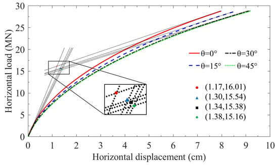
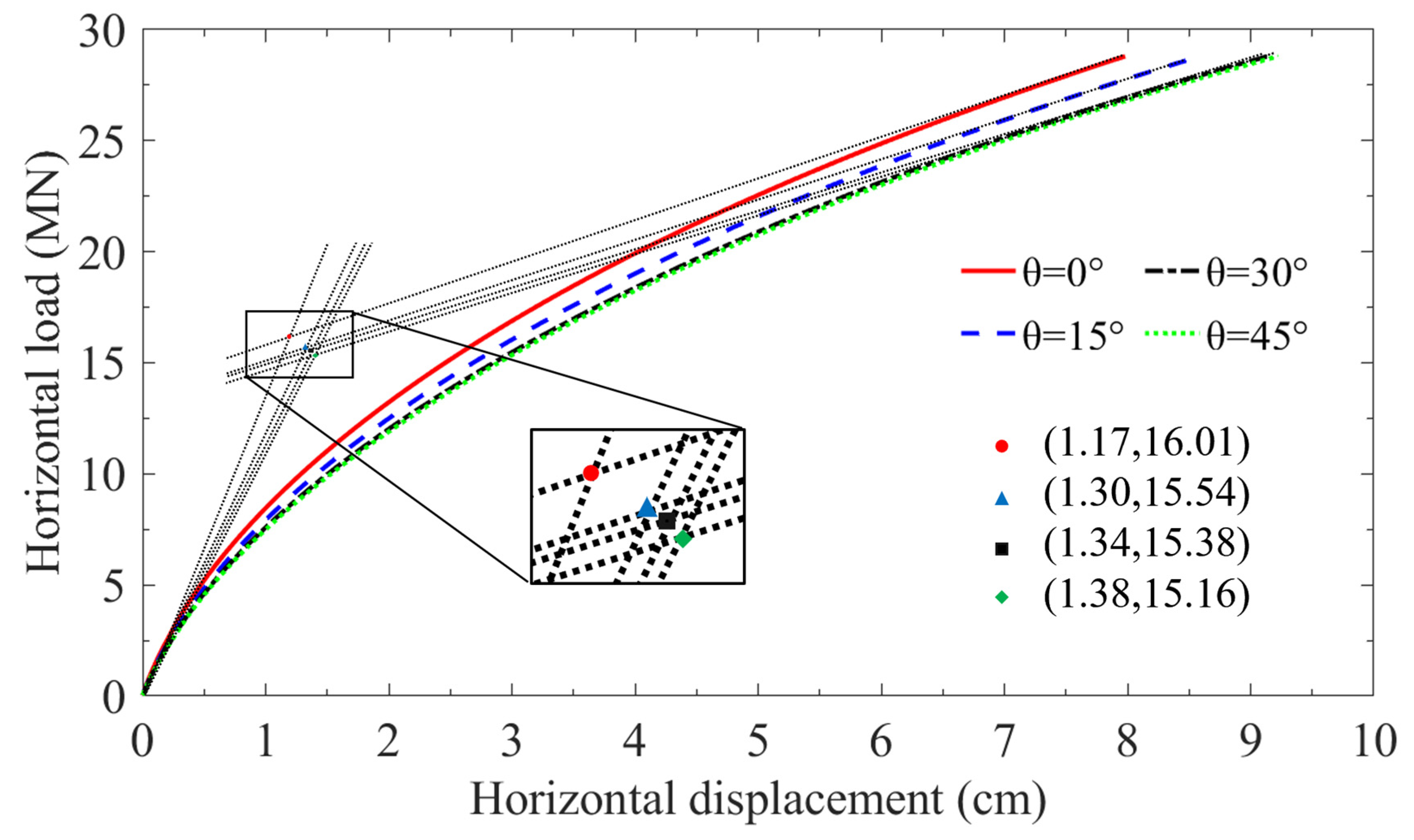
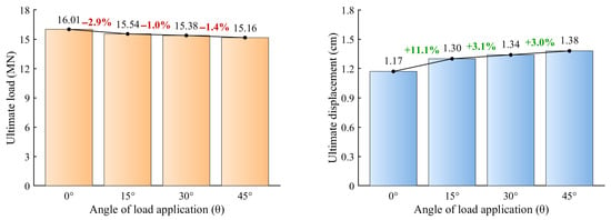
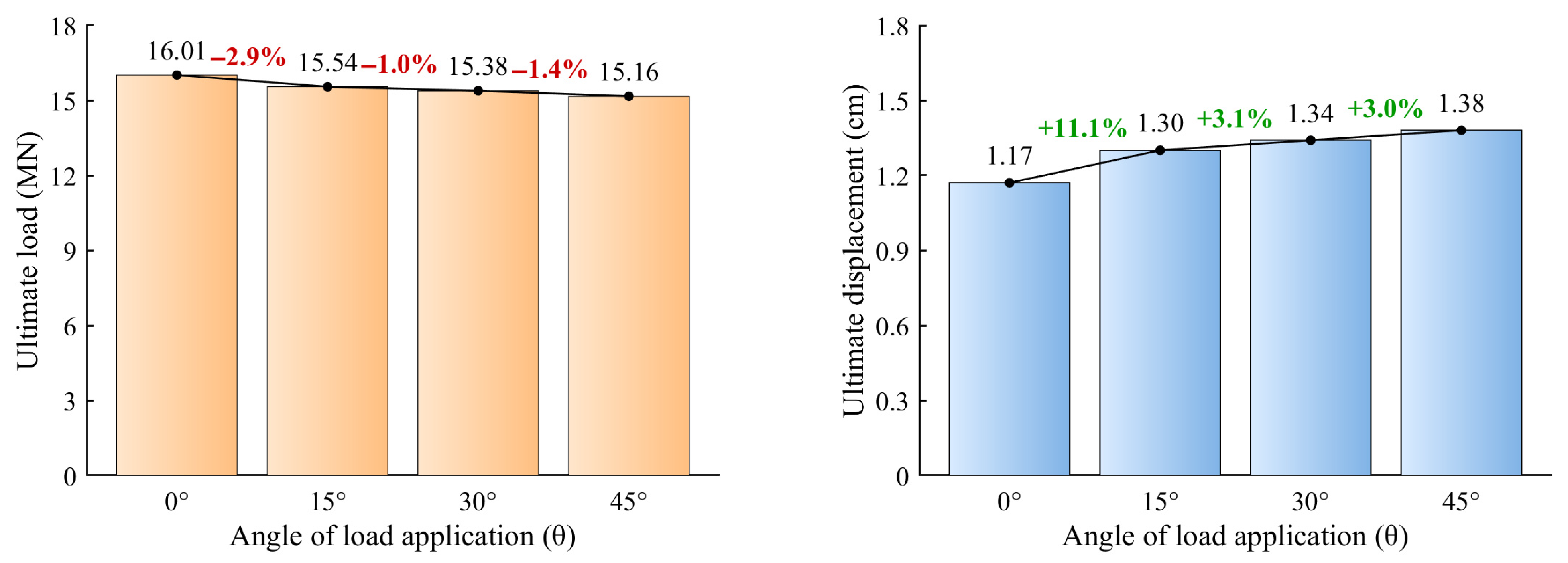
To evaluate the ultimate bearing capacity of the jacket foundation under different loading angles, the horizontal displacement at a reference point K on Pile C, which exhibits the most significant displacement change, is selected as the representative. The load–displacement curves are plotted, and the ultimate bearing state in each case is determined using the double-tangent intersection method, as illustrated in Figure 12. The horizontal bearing capacity of the jacket foundation is approximately 15–16 MN. Figure 13 presents a bar chart of the loads and displacements at the ultimate bearing state for different loading angles. As the loading angle increases, the ultimate bearing capacity shows a decreasing trend. Compared to that in the $\theta$ = 0° case, the ultimate horizontal bearing capacity in the $\theta$ = 45° case decreases by approximately 5.3%, representing the most unfavorable load condition. Therefore, the bearing state of the four-monopile jacket foundation under the $\theta$ = 45° loading condition should be prioritized in engineering design.

Figure 12. Ultimate bearing behavior of the jacket foundation taking Pile C as the representative.

Figure 13. Ultimate bearing capacity and displacement with loading angle.

5.2.2. Vertical Displacement

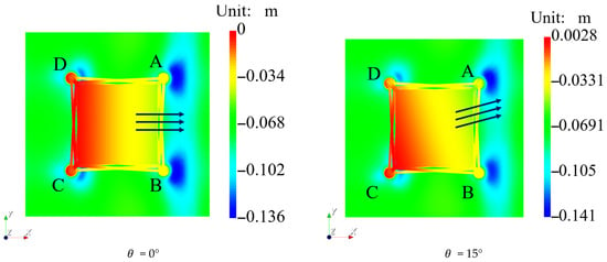
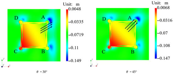
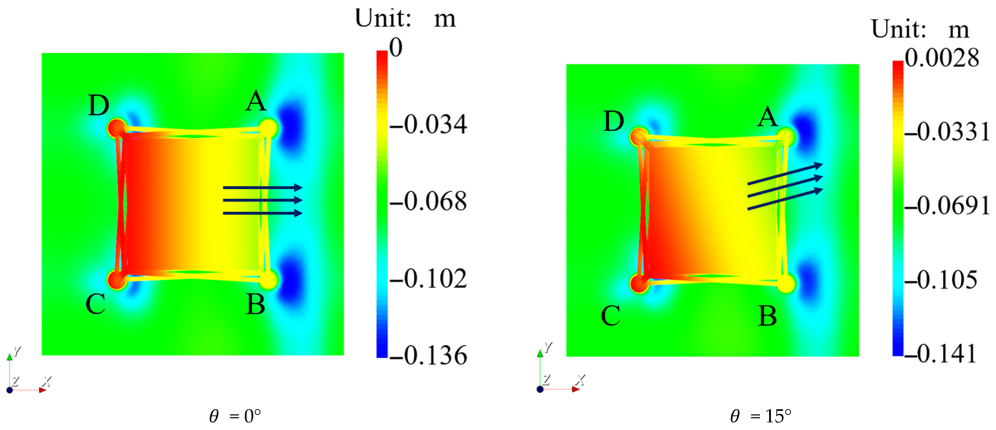
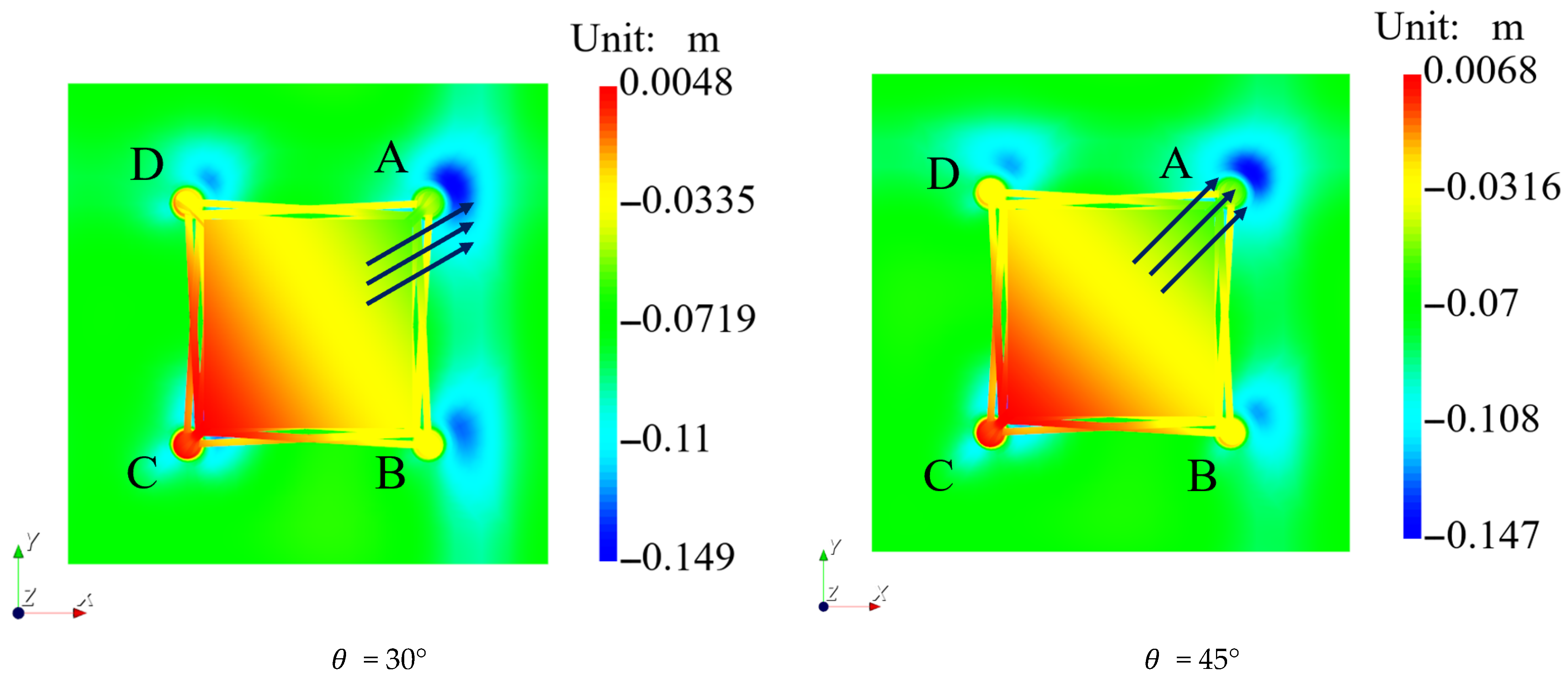
Figure 14 illustrates the displacement distribution of the jacket foundation in the Z-direction at the final loading (F = 28.8 MN) under different loading angles. At $\theta$ = 0°, the foundation displacement and soil settlement exhibit strict symmetry about the X-axis. In this state, the piles on the right side (Piles A and B) are both under compression, jointly resisting the overturning, and the settlement magnitude and range of the soil surrounding Piles A and B are significantly greater than those surrounding Piles C and D. At $\theta$ = 15°, the symmetry of the vertical displacement distribution is broken. The compressive load borne by Pile A gradually increases relative to that on Pile B, the zone of maximum settlement shifts towards the soil surrounding Pile A, and an uplift trend becomes apparent for Pile C. At $\theta$ = 30°, the soil settlement around Pile A further increases, the pressure distribution around Piles B and D approaches symmetry, and the uplift displacement of Pile C is further magnified. At $\theta$ = 45°, where the loading direction is perfectly aligned with the diagonal connecting Piles A and C, the overall vertical displacement contour plot enters a new symmetric state with the diagonal line as the axis of symmetry. In this state, the soil settlement around Pile A reaches its maximum value of approximately 0.147 m. Piles B and D, located symmetrically in the middle and perpendicular to the loading direction, have essentially equal displacement magnitudes, while Pile C exhibits the most significant uplift state.

Figure 14. Bird’s-eye view of the distribution of vertical displacement of the jacket foundation and its seabed foundation at F = 28.8 MN. (The arrow means the direction of load action, and ABCD represents the single pile number).

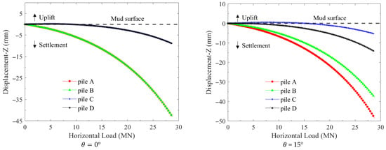
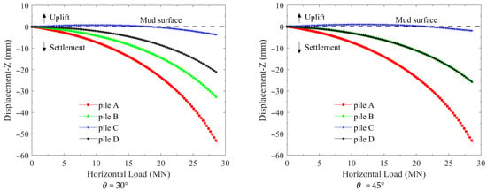
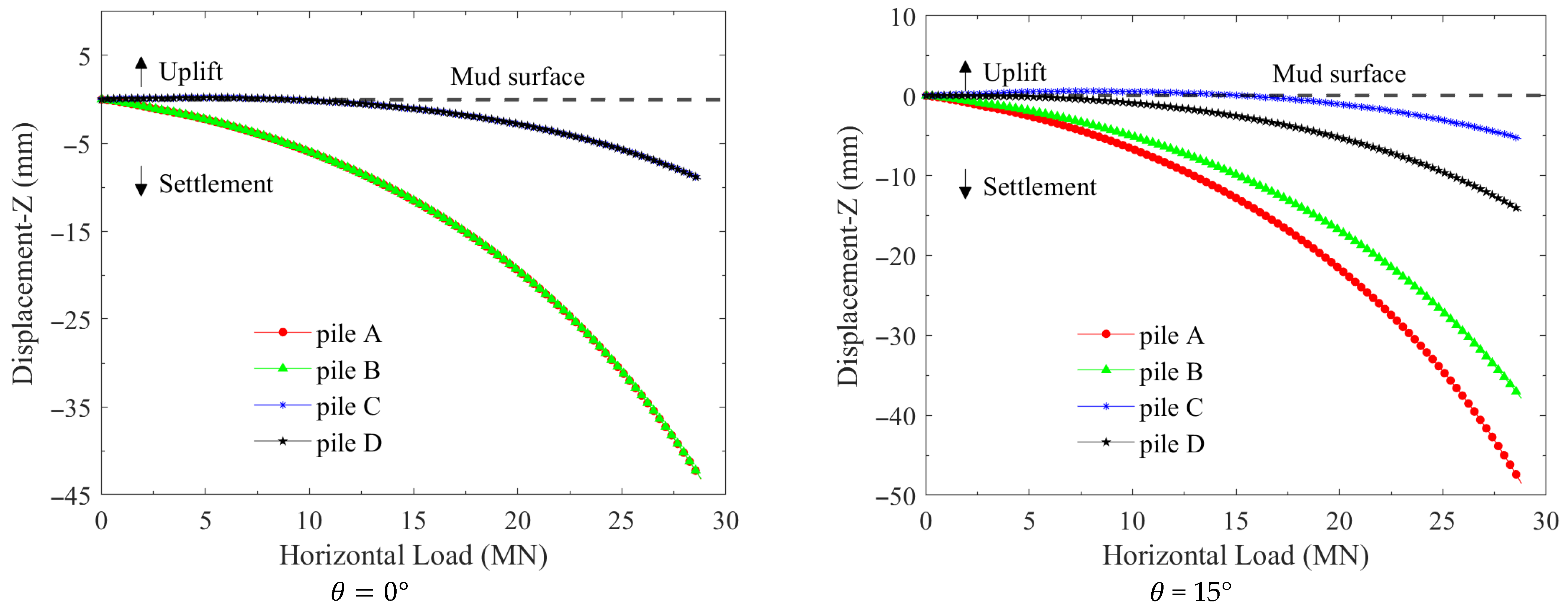
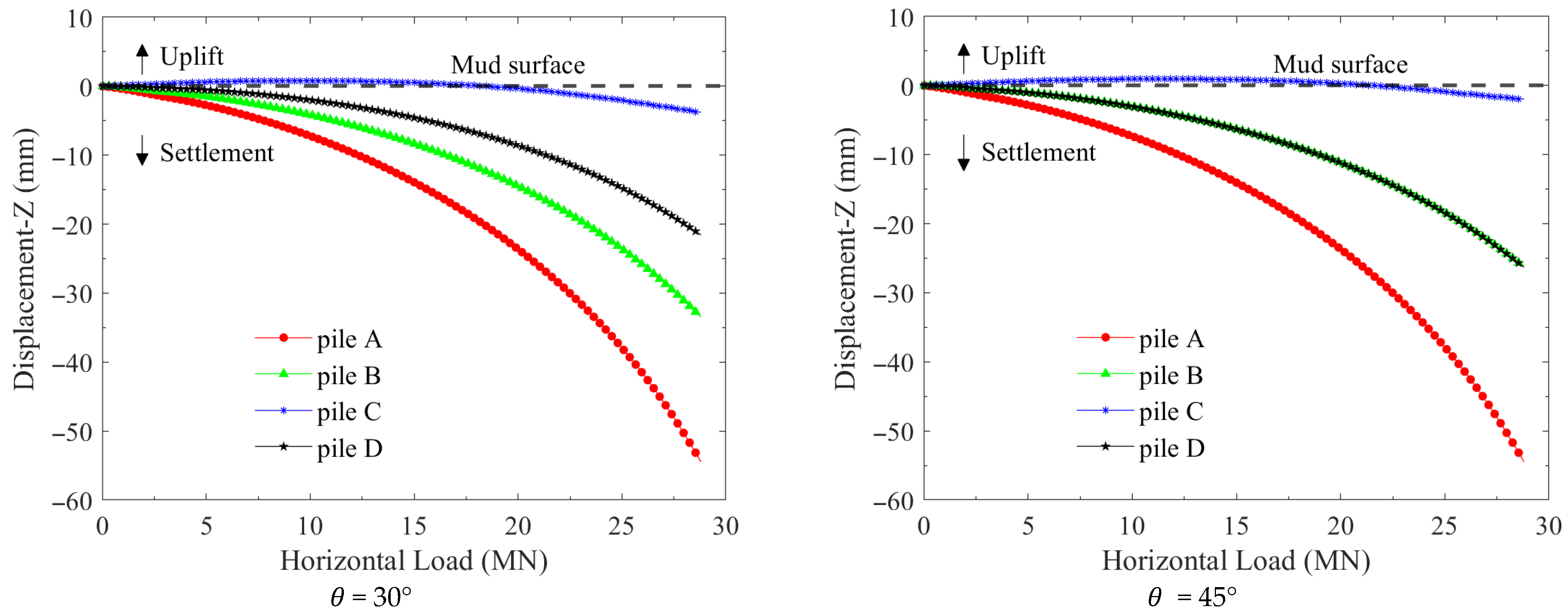
The vertical displacement–load response curves at the four points M, N, K, and L are extracted and presented in Figure 15. At $\theta$ = 0°, the displacement curves for the pile pairs A and B and C and D completely overlap, reflecting the symmetry of the displacement contour plotting about the X-axis. During the initial loading stage (F = 0 to 8 MN), Piles C and D exhibit an initial uplift, followed by settlement. This behavior is attributed to the overall rigid-body rotation of the jacket foundation under small loads, which induces minor uplift of Piles C and D. As the load increases, a portion of the soil around the piles enters a plastic yielding state, causing the overall settlement effect to gradually become dominant, thereby counteracting the initial uplift component and leading the vertical displacement to eventually transition into settlement. At $\theta$ = 0° and $\theta$ = 15°, the displacement curves for each pile are similar. In all cases, Pile A, being closer to the point of loading application, exhibits a significantly faster settlement rate, while the settlement trends of Piles B and D gradually become identical. At $\theta$ = 45 °, the final settlement at the head of Pile A reaches approximately −55 mm. The vertical displacement curves for Piles B and D completely coincide under this loading case. The uplift phase for Pile C is significantly prolonged compared to that in the $\theta$ = 0° case, only transitioning to settlement in the middle-to-late stage of loading (at F = 20 MN).

Figure 15. Evolution of vertical displacement at the pile heads versus horizontal loading.

6. Conclusions

Based on the theory of the HSS model and the implicit return mapping algorithm, the HSS model was numerically implemented and validated within the framework of the finite element software FssiCAS by utilizing the Fortran programming language. Furthermore, the horizontal bearing characteristics of a four-monopile jacket foundation–seabed foundation for an offshore wind turbine under various horizontal loading angles are explored adopting FssiCAS incorporating the HSS model. Based on the computational results, the following recognitions are obtained:

(1)

Validation through triaxial elemental tests and physical model tests of a laterally loaded monopile demonstrates that the HSS constitutive model, as numerically implemented in the marine geotechnics software FssiCAS, possesses excellent reliability and robustness within the parametric scope of this study.

(2)

The lateral ultimate bearing capacity of the four-monopile jacket foundation–seabed system is moderately affected by the horizontal loading angle, with the variation being within 10% (dropping from 16.01 MN to 15.16 MN). The ultimate bearing capacity is at its minimum when the jacket is loaded along the diagonal direction of the four monopiles. Consequently, this critical loading case should be used to evaluate the horizontal bearing capacity of the system, which is conservative for the engineering safety margin.

(3)

The numerical software FssiCAS for marine geotechnics demonstrates high applicability and robustness in addressing complex pile–soil interaction problems, such as the bearing capacity of jacket foundations involving intricate geometries and complex mechanical behaviors of seabed soils. It could serve as a valuable analysis platform for the optimization design of offshore wind power structures.

References

- Atkinson, J.H. Experimental determination of stress-strain-time characteristics in laboratory and in situ tests. In Proceedings of the 10th European Conference Soil Mechanics and Foundation Engineering; General Report; CRC: Florence, Italy, 1991; pp. 915–956. [Google Scholar]
- Jardine, R.; Potts, D.; Fourie, A.; Burland, J.B. Studies of the influence of non-linear stress–strain characteristics in soil–structure interaction. Geotechnique 1986, 36, 377–396. [Google Scholar] [CrossRef] [Scilit]
- Mair, R. Developments in geotechnical engineering research: Application to tunnels and deep excavations. In Proceedings of the Institution of Civil Engineers; Civil Engineering; Institution of Civil Engineers: London, UK, 1993; pp. 27–41. [Google Scholar]
- Zhu, F.; Zhang, M.; Ma, F.; Li, Z.; Qu, X. Identification of wind load exerted on the jacket wind turbines from optimally placed strain gauges using C-optimal design and mathematical model reduction. J. Mar. Sci. Eng. 2024, 12, 563. [Google Scholar] [CrossRef] [Scilit]
- Lundquist, J.K.; Clifton, A.J.; Dana, S.; Huskey, A.; Moriarty, P.; van Dam, J.; Herges, T. Wind Energy Instrumentation Atlas; National Renewable Energy Lab. (NREL): Golden, CO, USA, 2019. [Google Scholar]
- Ali, A.; Risi, R.; Sextos, A.; Goda, K.; Chang, Z. Seismic Vulnerability of Offshore Wind Turbines to Pulse and Non-Pulse Records. Earthq. Eng. Struct. Dyn. 2019, 49, 24–50. [Google Scholar] [CrossRef] [Scilit]
- Roscoe, K.H.; Burland, J.B. On the Generalized Stress-Strain Behaviour of Wet Clay; Engineering plasticity; Cambridge University Press: Cambridge, UK, 1968. [Google Scholar]
- Schanz, T.; Vermeer, P.; Bonnier, P.G. The hardening soil model: Formulation and verification. In Beyond 2000 in Computational Geotechnics; Routledge: London, UK, 2019; pp. 281–296. [Google Scholar]
- Duncan, J.M.; Chang, C.-Y. Nonlinear analysis of stress and strain in soils. J. Soil Mech. Found. Div. 1970, 96, 1629–1653. [Google Scholar] [CrossRef] [Scilit]
- Chen, J.Y.; Teng, J.C.; Wu, Z.X. Numerical simulation of failure envelope of suction bucket foundation in clay. J. Civ. Environ. Eng. 2022, 44, 45–51. (In Chinese) [Google Scholar]
- Yin, Z.-Y.; Teng, J.-C.; Li, Z.; Zheng, Y.-Y. Modelling of suction bucket foundation in clay: From finite element analyses to macro-elements. Ocean. Eng. 2020, 210, 107577. [Google Scholar] [CrossRef] [Scilit]
- Demirci, H.E. Numerical Evaluation of Hybrid Foundation Efficiency for Offshore Wind Turbines. Geotech. Geol. Eng. 2025, 43, 167. [Google Scholar] [CrossRef] [Scilit]
- Kou, H.L.; Fang, W.W.; Xu, X.C.; An, Z.; Zhang, H.R. Comparative study on horizontal cyclic bearing characteristics of offshore wind power bucket foundation based on HSS model. Ocean. Eng. 2024, 42, 1–12. (In Chinese) [Google Scholar]
- Du, W. Image Analysis for Determination of Triaxial Test Parameters. Doctoral Dissertation, The University of Western Australia, Crawley, WA, Australia, 2024. [Google Scholar]
- Wang, C.F. Study on Deformation Law and Construction Deformation Control of Dewatering Excavation of a Granite Residual Soil Foundation Pit. Master’s Thesis, South China University of Technology, Guangzhou, China, 2023. (In Chinese) [Google Scholar]
- Hashash, Y. Analysis of Deep Excavations in Clay. Ph.D. Thesis, Massachusetts Institute of Technology, Cambridge, MA, USA, 1992. [Google Scholar]
- Tang, D.F.; Wang, C.H. Development and application of small-strain hardening soil constitutive model in FLAC3D. J. Shanghai Univ. Nat. Sci. Ed. 2023, 29, 549–561. (In Chinese) [Google Scholar]
- Cocco, L.; Ruiz, M. Numerical implementation of hardening soil model. In Numerical Methods in Geotechnical Engineering IX, Volume 1; CRC Press: Boca Raton, FL, USA, 2018; pp. 195–203. [Google Scholar]
- Ye, J.; Jeng, D.; Wang, R.; Zhu, C. Validation of a 2-D semi-coupled numerical model for fluid–structure–seabed interaction. J. Fluids Struct. 2013, 42, 333–357. [Google Scholar] [CrossRef] [Scilit]
- Ye, J. Numerical Analysis of Wave-Seabed-Breakwater Interactions. Doctoral Thesis, University of Dundee, Dundee, Scotland, 2012. [Google Scholar]
- Yao, Y.-P.; Liu, L.; Luo, T.; Tian, Y.; Zhang, J.-M. Unified hardening (UH) model for clays and sands. Comput. Geotech. 2019, 110, 326–343. [Google Scholar] [CrossRef] [Scilit]
- Elgamal, A.; Yang, Z.; Parra, E.; Ragheb, A. Modeling of cyclic mobility in saturated cohesionless soils. Int. J. Plast. 2003, 19, 883–905. [Google Scholar] [CrossRef] [Scilit]
- Ye, J.; Jeng, D.; Chan, A.H.C. Consolidation and dynamics of 3D unsaturated porous seabed under rigid caisson breakwater loaded by hydrostatic pressure and wave. Sci. China Technol. Sci. 2012, 55, 2362–2376. [Google Scholar] [CrossRef] [Scilit]
- Ye, J.; Jeng, D.-S.; Liu, P.-F.; Chan, A.; Wang, R.; Zhu, C.-Q. Breaking wave-induced response of composite breakwater and liquefaction in seabed foundation. Coast. Eng. 2014, 85, 72–86. [Google Scholar] [CrossRef] [Scilit]
- Ye, J.; He, K. Dynamics of a pipeline buried in loosely deposited seabed to nonlinear wave & current. Ocean. Eng. 2021, 232, 109127. [Google Scholar]
- He, K.; Ye, J. Dynamics of offshore wind turbine-seabed foundation under hydrodynamic and aerodynamic loads: A coupled numerical way. Renew. Energy 2023, 202, 453–469. [Google Scholar] [CrossRef] [Scilit]
- Schanz, T. A constitutive model for hard soils. Geotech. Hard Soils-Soft Rocks 1998, 2, 861–868. [Google Scholar]
- Lade, P.V. Modelling the strengths of engineering materials in three dimensions. Mech. Cohesive-Frict. Mater. 1997, 2, 339–356. [Google Scholar] [CrossRef]
- Benz, T. Small-Strain Stiffness of Soils and Its Numerical Consequences. Master’s Thesis, University of Stuttgart—Institute of Geotechnical Engineering, Stuttgart, Germany, 2007. [Google Scholar]
- Li, X.S.; Dafalias, Y.F. Dilatancy for cohesionless soils. Géotechnique 2000, 50, 449–460. [Google Scholar] [CrossRef] [Scilit]
- Sivasithamparam, N. Development and Implementation of Advanced Soft Soil Models in Finite Elements. Ph.D. Thesis, University of Strathclyde, Glasgow, Scotland, 2012. [Google Scholar]
- Sivasithamparam, N.; Castro, J. An anisotropic elastoplastic model for soft clays based on logarithmic contractancy. Int. J. Numer. Anal. Methods Geomech. 2016, 40, 596–621. [Google Scholar] [CrossRef] [Scilit]
- Bonnier, P. Implementational aspects of constitutive modeling. SCMEP Workshop No 1 at NTNU, August 2000. [Google Scholar]
- Simo, J.C.; Taylor, R.L. Consistent tangent operators for rate-independent elastoplasticity. Comput. Methods Appl. Mech. Eng. 1985, 48, 101–118. [Google Scholar] [CrossRef]
- Koiter, W.T. General Theorems for Elastic-Plastic Solids. Master’s Thesis, Delft University of Technology, Delft, The Netherlands, 1960. [Google Scholar]
- Liao, J.; Zhu, Q.C.; Wang, Z.J.; Dai, Z. Simulation and comparison of effects of advanced and commonly used constitutive models on loess deformation. Chin. J. Undergr. Space Eng. 2023, 19, 784–792. (In Chinese) [Google Scholar]
- Fei, K.; Zhang, J.W. Application of ABAQUS in Geotechnical Engineering; China Water & Power Press: Beijing, China, 2010. (In Chinese) [Google Scholar]
- Jakobsen, K.P. Application of the Single Hardening Model in the Finite Element Program ABAQUS; China Water & Power Press: Beijing, China, 1999. [Google Scholar]
- Wang, S.; Wu, W. A simple hypoplastic model for overconsolidated clays. Acta Geotech. 2021, 16, 21–29. [Google Scholar] [CrossRef] [Scilit]
- Chen, H. Study on Horizontal Bearing Capacity and Deformation Characteristics of Monopile Foundations for Offshore Wind Turbines. Master’s Thesis, Zhejiang University of Technology, Hangzhou, China, 2018. (In Chinese) [Google Scholar]
- Trochanis, A.M.; Bielak, J.; Christiano, P. Three-Dimensional Nonlinear Study of Piles. J. Geotech. Eng. 1991, 117, 429–447. [Google Scholar] [CrossRef] [Scilit]
- Liang, F.Y.; Jia, Y.J.; Ding, Y.J.; Huang, M. Experimental study on parameters of HSS model for soft soils in Shanghai. Chin. J. Geotech. Eng. 2017, 39, 269–278. (In Chinese) [Google Scholar]
- Zhu, B.; Wen, K.; Li, T.; Wang, L.; Kong, D. Experimental study on lateral pile–soil interaction of offshore tetrapod piled jacket foundations in sand. Can. Geotech. J. 2019, 56, 1680–1689. [Google Scholar] [CrossRef] [Scilit]
- Zhu, B.; Wen, K.; Kong, D.; Zhu, Z.; Wang, L. A numerical study on the lateral loading behaviour of offshore tetrapod piled jacket foundations in clay. Appl. Ocean. Res. 2018, 75, 165–177. [Google Scholar] [CrossRef] [Scilit]
- Wang, B.; Qin, T.; Yuan, C.; Li, L.; Yuan, M.; Li, Y. Analysis of bearing performance of monopile and single suction bucket foundation for offshore wind power under horizontal load. Geofluids 2022, 2022, 4163240. [Google Scholar] [CrossRef] [Scilit]
- NB/T 10105-2018; Code for Design of Foundations for Offshore Wind Farm Projects. National Energy Administration of China: Beijing, China, 2018. (In Chinese)
- Yavari, N. Aspects Géotechniques des Pieux de Fondation Énergétiques. Doctoral Dissertation, Université Paris-Est, Paris, France, 2014. [Google Scholar]
- Zhao, L.; Sun, M.; Ye, J.; Yang, F.; He, K. Characteristics and Rapid Prediction of Seismic Subsidence of Saturated Seabed Foundation with Interbedded Soft Clay–Sand. J. Mar. Sci. Eng. 2025, 13, 559. [Google Scholar] [CrossRef] [Scilit]
- Yuan, J.; Chen, X.; Gu, X.; Lin, Y.; Jiao, J.; Wu, C. Experimental study on parameters of small strain hardening soil model for marine sandy soil in Yangjiang, Guangdong. J. Tongji Univ. Nat. Sci. 2022, 50, 852–860. (In Chinese) [Google Scholar]
Disclaimer/Publisher’s Note: The statements, opinions and data contained in all publications are solely those of the individual author(s) and contributor(s) and not of MDPI and/or the editor(s). MDPI and/or the editor(s) disclaim responsibility for any injury to people or property resulting from any ideas, methods, instructions or products referred to in the content. |
© 2026 by the authors. Licensee MDPI, Basel, Switzerland. This article is an open access article distributed under the terms and conditions of the Creative Commons Attribution (CC BY) license.