


Abstract
Coupled climate models integrate atmospheric, oceanic, and land submodels, while the uncertainty of model parameters from different parameterization schemes or empirically derived parameters inevitably introduces systematic biases. Coupled parameter optimization (CPO) can reduce these biases to improve weather forecast and climate prediction, but must address strong nonlinearities inherent in coupled models. The analytical four-dimensional ensemble variational (A-4DEnVar) data assimilation method retains the nonlinear processing capability of the four-dimensional variational (4D-Var) data assimilation method but gets rid of the dependence on the adjoint model. In this study, a novel dynamic independent point (DIP) scheme is introduced to the improved A-4DEnVar, which reduces computational dimensionality and further explores a broader parameter space of dimensionality reduction through the outer loop. Based on the improved A-4DEnVar, a series of geographic-dependent CPO experiments with an idealized 2D coupled model are carried out. Results show that A-4DEnVar accurately captures the geographical characteristics of parameters and effectively optimizes cross-component parameters despite strong nonlinearity. Additionally, the DIP scheme presents significant advantages compared to the static independent point scheme, especially with fewer independent points. This work is offering a new perspective for parameter optimization in coupled general circulation models used for climate estimation and prediction.
1. Introduction
Coupled Earth system models (ESMs) play an increasingly important role in reanalysis and climate prediction, and how to further improve its simulations and forecasting abilities has become a popular research issue. There are two key factors affecting the simulations and predictions of a coupled model: the quality of initial conditions of the coupled model states, and the coupled model biases. Coupled data assimilation (CDA) aims to provide dynamically consistent initial conditions by allowing information from one component to influence the analysis of another within the coupled model [1,2,3,4,5]. However, the existence of systematic error [6,7] could lead to model predictions drifting towards an imperfect model climate [8], and coupled modeling is no exception. As an essential resource of systematic error, model bias significantly influences the accuracy of data assimilation and numerical forecasting [9,10,11,12,13,14,15]. The mentioned model bias usually originates from an imperfect dynamical core and the physical parameterizations [12]. The errors in physical parameterizations arise from both the structural uncertainty in their formulation and the empirical settings of model parameters. In the case of a coupled model, it also includes coupled coefficients involving the interaction of the coupled components. Therefore, parameter optimization for coupled models naturally falls within the scope of CDA. This specific application is termed coupled parameter optimization (CPO). The optimization of parameters within a single component falls into weakly coupled data assimilation (WCDA). In contrast, optimizing cross-component coupled parameters belongs to the category of strongly coupled data assimilation (SCDA), as it inherently addresses the core interactions between model components [5]. This conceptual foundation, which focuses on handling interactions across model components, has been most concretely realized through the SCDA framework. Kitsios et al. [16] successfully performed geographic-dependent parameter estimation for ocean optical properties within SCDA framework. However, their focus was on optimizing parameters internal to a single model component (e.g., the ocean). In fact, while the SCDA approach has proven powerful for estimating component-internal parameters, there are fewer studies on its application to cross-component parameter optimization [1].
Another issue to be noted is that in most studies of CPO, the parameters are usually simply set as globally uniform without any geographic-dependent characteristics. In another word, the parameter values are the same across the entire area of research. Such a simplified approach makes it impossible to accurately estimate the geographic characteristics of the parameter in coupled model. As some studies [13,14] pointed out, taking into account the spatial distribution characteristics of the parameter in the coupled model when carrying out CPO can further reduce the model bias compared to single-value parameter optimization, and thus obtain better climate estimation and prediction. Note that most studies in geographic-dependent parameter optimization (GPO) are conducted based on a data assimilation scheme for enhancive parameter correction [12] with ensemble filtering. Crucially, these studies primarily address the spatial patterns of parameter sensitivity derived from ensemble-based methods. In contrast, the focus of the present work is on obtaining the real geographic characteristics of the parameters by optimization, which is crucial for enhancing climate simulations and reanalysis.
For the implementation of parameter optimization, ensemble filtering [12,13,17,18,19] and variational data assimilation [20,21,22,23,24,25] methods have been widely adopted. Kalnay et al. [26] argued that the ensemble Kalman filter (EnKF) performs better with short assimilation windows, whereas the four-dimensional variational (4D-Var) data assimilation method can achieve similar accuracy with longer windows and is more effective in handling model errors. Nowadays, hybrid methods that combine ensemble filtering and 4D-Var, such as En4DVar [27] and 4DEnVar [28], are also widely studied [29,30,31]. On the one hand, En4DVar optimizes the solution of the background error covariance matrix, but it still depends on the complex adjoint model, similar to 4D-Var. On the other hand, while 4DEnVar avoids the adjoint model, it struggles to retain the nonlinear processing capability of 4D-Var because of the linear correlation between the perturbations of states and observations assumed in 4DEnVar [32]. In response to the issue, Liang et al. [33] combined the explicit flow-dependent background error covariance of ensemble assimilation with the strong dynamic constraints of 4D-Var, and presented the analytical four-dimensional ensemble variational (A-4DEnVar). A-4DEnVar utilizes the dynamical model evolution information contained in a sufficiently small but diverse ensemble to simulate the tangent linear and adjoint models. It implicitly integrates evolution information through time-cross covariance matrices, bypassing explicit operator of the tangent linear construction and leveraging the intrinsic mathematical property. Furthermore, the method not only avoids the adjoint model, but also sufficiently inherits the capability of processing nonlinear issues that normally exists in coupled models. The assimilation performance of A-4DEnVar has been initially investigated using the Lorenz-63 model [33]. Furthermore, Liang et al. [34] applied A-4DEnVar in an ocean circulation model and succeeded in estimating the bottom friction coefficient with spatial distribution characteristics in the Bohai and Yellow Seas. They firstly introduced an independent point scheme to further reduce computational cost, demonstrating the effectiveness of A-4DEnVar in estimating spatial distribution parameters. Considering the promising assimilation potential of A-4DEnVar, Gong et al. [35] conducted CPO for an idealized 1D coupled model based on Lorenz-63, finding that A-4DEnVar has similar performance to 4D-Var, particularly with a longer data assimilation window. Ensemble-based variational methods face a fundamental challenge of rank deficiency when applied to high-dimensional systems, a problem intrinsically rooted in the computational infeasibility of maintaining full rank with limited resources. To address this fundamental and persistent challenge, we introduce innovative improvements to the A-4DEnVar framework. One improvement involves a sample-space variable replacement algorithm. It significantly reduces computational complexity and transforms the computational dimensionality into the sample space. On the other hand, to achieve dimensionality reduction in parameter optimization, a novel dynamic independent point (DIP) scheme is presented in this paper, in contrast to the static independent point (SIP) scheme used by Liang et al. [34].
Significantly, this paper presents the first application of A-4DEnVar to geographical-dependent CPO, particularly for cross-component coupled parameter optimization under a SCDA framework. Furthermore, although both SIP and DIP schemes can achieve the dimension reduction in the parameter optimization, the DIP scheme integrates the SIP scheme with the outer-loop mechanism of A-4DEnVar and allows the locations of IPs to be updated before each outer-loop iteration. This allows the global solution to be not solely restricted to SIPs, but instead explores a broader parameter space of dimensionality reduction through the outer loop. This work systematically conducts CPO experiments and assesses multiyear forecasts using an idealized atmosphere–ocean–land coupled model. Considering that this work focuses on systematically evaluating the performance of geographic-dependent parameter optimization based on A-4DEnVar under a SCDA framework, we presented perfect initial conditions for the model, eliminating the requirement for state estimation, such that model biases originate exclusively from parameters. A series of idealized parameter optimization experiments are then conducted under these controlled conditions.
The paper is organized as follows. Section 2 introduces the strategy of parameter optimization based on A-4DEnVar as well as DIP scheme. Section 3 provides a brief introduction to the idealized coupled model. Section 4 describes the settings of twin experiments and evaluates the performance of geographical-dependent CPO based on A-4DEnVar with DIP scheme. Its implications for climate simulations and predictions are also investigated in Section 4. Section 5 presents a discussion of the results and their broader implications. Finally, the main conclusions are summarized in Section 6.
2. Methodology
2.1. Parameter Optimization Scheme Based on A-4DEnVar
When performing data assimilation, 4D-Var searches the minimum value of the cost function with respect to the control variable to obtain the optimal analysis value. The control variable can be either the initial model state or the parameter, depending on whether the optimization is focused on the initial conditions or the parameters. Note that the parameter can be regarded as the augmented state variable that does not change with time and has no observation [36]. Linearizing about the first guess state for the control vector, we introduce the deterministic component and a small increment of control variable (i.e., and ). This decomposition follows the incremental approach of 4D-Var [37], transforming a global nonlinear optimization problem into a local linear problem of finding an optimal small perturbation near a known background field. The general form of the cost function with respect to the first guess control variable () can be represented as
where denotes the background control variable at the initial time , and the control variable noted here includes both state and parameter; is the background error covariance matrix; denotes the observation operator at (i.e., the current analysis time step) from state space to observational space; denotes the predictive model operator from to ; and indicate the observations and their error covariance, respectively; and denotes the number of observations. Thus, the gradient of the cost function with respect to is
where and respectively denote the tangent linear model and its adjoint model of . Note that 4D-Var is highly dependent on the adjoint model (i.e., ), which is one of the reasons for high computational cost. By incorporating the concept of A-4DEnVar, the issues can be effectively resolved, which is explained as follows.
To derive the subsequent formulations, we split the previously mentioned control variable (i.e., ) into two parts: the model parameters and the state variable . Assuming no external forcing, the evolution of model state through the numerical dynamic model can be represented as follows:
where denotes the state vector at , and represents the parameter vector which is set at and used in the model evolution from to . To investigate the evolution of state uncertainty and the relationship between state and parameter uncertainties during the dynamic evolution, the deterministic component and the perturbation of (i.e., and ) along with the deterministic component and the perturbation of (i.e., and ) are introduced. We denote as the number of elements in the state vector , and as the number of elements in the parameter vector . Then, the “perturbed” model state can be represented as
where is constant during the model evolution in our study. The first-order Taylor expansion expression of Equation (4) around is
Here, (a matrix) and (a matrix) denote the tangent linear operators of the predictive model around with regard to and , respectively; and denotes the higher-order terms of the expansion. The perturbations are designed to be sufficiently small, governed by a key scaling factor (whose specific role is detailed later in Equation (11). This ensures that is negligibly small compared to the retained first-order term, thus justifying its omission in the subsequent derivation. Theoretically, the complete Taylor expansion remainder should include the partial derivatives between parameters; however, these terms can be neglected because we assume that is time invariant and that the parameters at different locations are mutually independent.
As our study solely focuses on parameter optimization, is assumed to be unbiased and will not be optimized, while any bias of the coupled system is only resourced from . Therefore, either , the directional derivative of with respect to (i.e., ), or the mixed partial derivatives of in is, in practice, non-existent. In contrast, the directional derivative with respect to (i.e., ) is crucial for representing the response of at (i.e., ) to . Consequently, Equation (5) legitimately simplifies. By further combining Equation (5) with , the state perturbation is approximately calculated by
We introduce the ensemble of , and the ensemble of , , in which is the ensemble size. Note that the dimension of and is and , respectively. Then, the ensemble-base state perturbation of can be expressed as follows:
It can be observed that the perturbation of the state variable during the model evolution is almost induced by the initial parameter perturbation. Furthermore, the relationship between their evolution is characterized by the tangent linear operator . If both sides of Equation (7) are right-multiplied by the transpose of the parameter perturbation ensemble (i.e., ), can be explicitly solved in the form of an expectation through derivation:
where exactly indicates the error covariance matrix of the ensemble parameter, that is
Thus, one can estimate utilizing the ensemble information from Equation (8), which is precisely the theoretical foundation for avoiding the adjoint model in A-4DEnVar. And on this basis, we next present the cost function and gradient of A-4DEnVar in parameter optimization.
According to Liang et al. [33], an adjustment term is sought in the vicinity of the initial guess to minimize the cost function. Thus, the cost function with respect to can be expressed as
where represents the background of ; and is the background error covariance matrix of the ensemble parameter. Note that the relationship of and in Equation (9) is assumed by
This relation formally defines the scaling factor that was pre-supposed in the generation of the parameter perturbation ensemble. The choice of a sufficiently small is the fundamental precondition that ensures the second and higher order term in Taylor expansion can be omitted, as shown by Equation (5). Equation (11) is a fundamental assumption of the method regarding the statistical property of the generated ensemble. This assumption links the theoretical covariance to the empirically computed sample covariance . Thus, we have
Due to the high computational cost associated with and the substantial computational storage requirements for constructing itself, this study adopts the following variable substitution (referred to as sample-space variable replacement), which can transform the computational space from control variable space to sample space:
Here, the transform term has the dimension of . Substituting Equations (12) and (13) into Equation (10), the cost function with respect to is transformed as follows:
Expanding the background term of Equation (14) and neglecting the term , as which is not used to calculate the gradient, we obtain the simplified cost function:
The inverse of the sample covariance matrix can be derived from its definition. Recall from Equation (9) that ; therefore, in Equation (15) can be expressed as
where and denote the pseudo-inverse of and , respectively. In order to deal with the pseudo-inverse in Equation (16), we first compute the eigenvalue decomposition of :
By left-multiplying both sides of Equation (17) by and then right-multiplying both sides by , we obtain
Subsequently, we can simultaneously left-multiply and right-multiply the expression on the right-hand side of Equation (16) by . Finally, can be simplified as
Substituting the above equation into Equation (15), we obtain
Finally, we derive the gradient of the cost function as
Note that to solve the above equation, the following expression is utilized according to
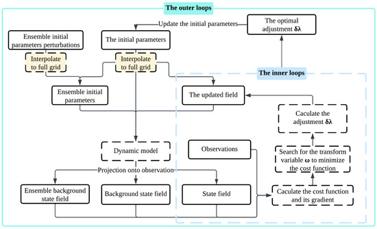
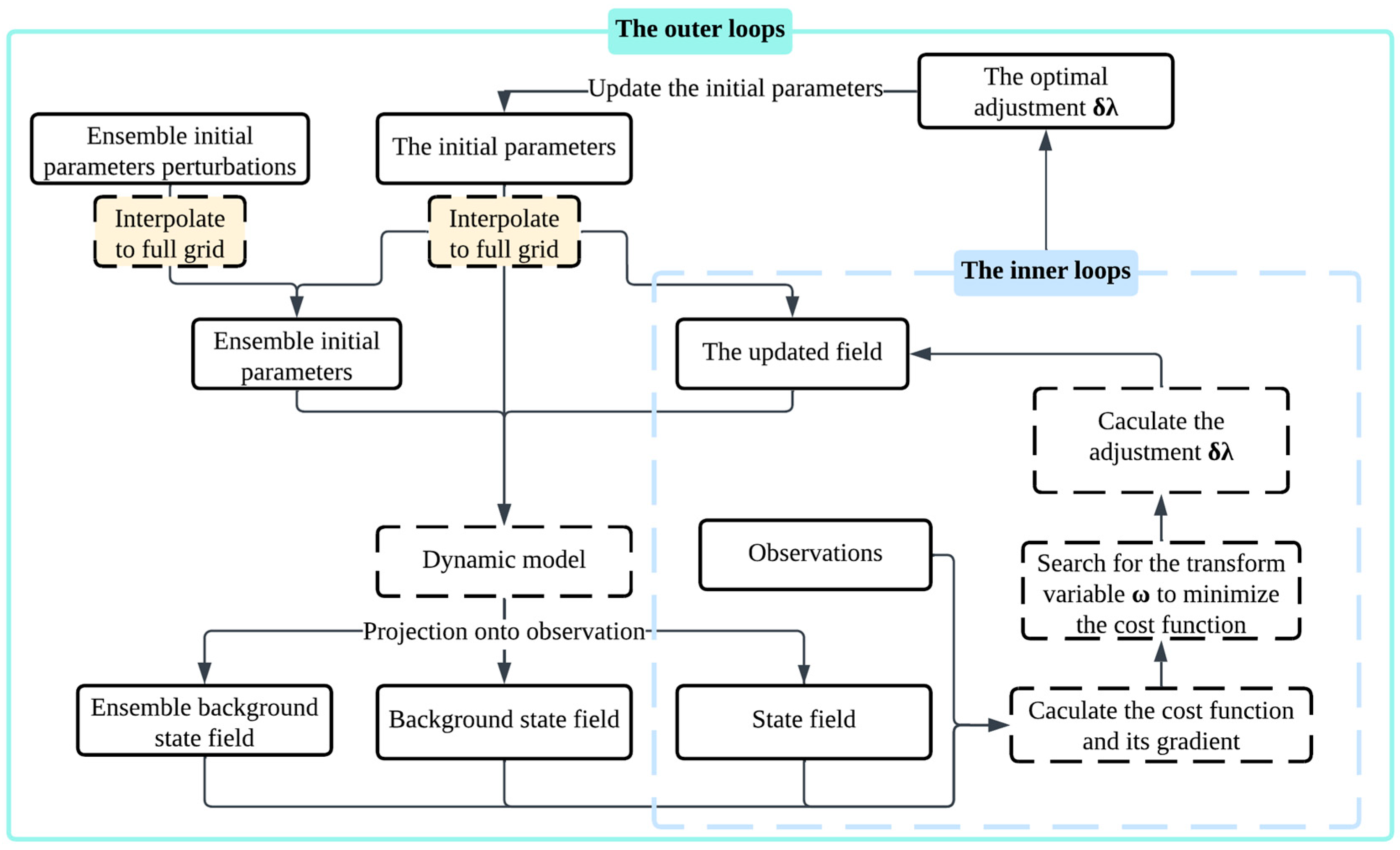
From Equation (21), the gradient can be calculated without requiring the tangent linear model, as it is approximated by an ensemble of perturbations, as shown in Equation (8), thereby dispensing with the adjoint model. This highlights the portability of A-4DEnVar. To avoid inaccuracies caused by excessive adjustment amounts, a linear search method is introduced, similar to the approach used in 4D-Var, to progressively adjust the first guess of . The L-BFGS-B method (limited-memory quasi-Newton method that approximates the Broyden–Fletcher–Goldfarb–Shanno algorithm for bound-constrained optimization) [38] is employed to find the optimal as well as . The risk of converging to the trivial solution is inherently mitigated, as the significant observational misfit from an imperfect initial parameter estimate creates a strong gradient that directs the optimizer toward a non-zero for meaningful parameter adjustment. Additionally, A-4DEnVar is designed as an outer–inner loop structure, in which the inner loop is responsible for the linear search, while the outer loop updates the first guess of (see Figure 1).
Figure 1.
Flow chart of A-4DEnVar for parameter optimization. A-4DEnVar is designed as an outer–inner loop structure, in which the inner loop is responsible for the linear search, while the outer loop updates the first guess of the parameter.
2.2. The Independent Point Scheme
As mentioned in the previous subsection, the improved A-4DEnVar transforms the computational dimensionality into the sample space through variable replacement, making it theoretically feasible for to be significantly smaller than . However, this approach of dimensionality reduction is primarily achieved in state estimation rather than in parameter optimization. This is because it imposes stricter demands on the independence of perturbations within the ensemble and requires high-quality ensemble samples that carry sufficient information to support the assimilation. For state variables, a feasible approach is generating such high-quality ensemble samples by utilizing their direct observational data; however, this is not viable for parameters. A rank-deficient initial ensemble, where the ensemble size is much smaller than the number of parameters, may fail to represent key directions of uncertainty. Therefore, to ensure a successful optimization, it is necessary to maintain an ensemble size comparable to the number of parameters (i.e., ), providing a sufficient basis for exploring and constraining the parameter space.
For parameter optimization, an effective dimensionality reduction method is still needed to meet the demands of operational applications. Liang et al. [34] applied a static independent point (SIP) scheme to parameter optimization based on A-4DEnVar. After a brief introduction for the SIP scheme, we present an improved scheme called dynamic independent point (DIP), to further enhance assimilation performance.
2.2.1. The Static Independent Point Scheme
Liang et al. [34] pointed out that the geographical-dependent characteristics of the model parameter to be optimized are typically determined by the parameter located at certain key positions, which can be named as independent points (IPs). As a result, only the parameters at IPs are directly optimized through data assimilation, while parameters at other grids are updated through spatial interpolation based on the parameters at IPs. The interpolation coefficients are determined by the distances between points, so that neighboring points exhibit similar values. Thus, the background parameter error covariance in the IP space is simplified to a quasi-diagonal matrix. It is evident that the application of IP significantly not only reduces the computational cost of parameter optimization but also introduces an implicit form of localization in data assimilation.
The SIP scheme does not alter the positions of IPs during the parameter optimization. The interpolation process employs the Cressman method [39], which can be described as follows:
where and denote the parameter value at the th grid point and the th IP, respectively; is the weight coefficient of the th IP with respect to the th grid point; indicates the distance from the th IP to the th grid point; represents the impact radius; and denotes the number of IPs. The interpolation process can be regarded as the “reverse” projection from IP space to model grid space. For clarity, we represent this process using the operator and use to represent the parameter field which is a vector composed of scalars after optimization at IPs. Therefore, the global parameter field which is a vector composed of scalars at all model grid points can be expressed as
2.2.2. The Dynamic Independent Point Scheme
As discussed by Liang et al. [34], the IPs should be selected to be sufficiently far apart. In essence, this means that the effectiveness of the independent point scheme applied in geographical-dependent parameter optimization (GPO) heavily relies on whether the selected IPs can provide key information elements on a global scale. But it is necessary to note that many model parameters lack explicit physical characteristics, which makes it difficult to identify the positions that provide critical global information. Although the issue could be addressed with the help of some methods such as the conditional nonlinear optimal perturbation (CNOP) scheme [40], it still requires considerable effort to research and diverges from the focus of this study.
Consequently, we first adopt a random selection method for determining IPs with constraints on the minimum distance: IPs are randomly selected within the full grid range, while imposing a constraint on the minimum distance between these IPs to ensure broad coverage across the domain. The minimum distance can be calculated as
where represents the area covered by all model grid cells. In this study, is equivalent to the impact radius (i.e., ) described in Equation (24). This approach allows for capturing geographical-dependent characteristics as effectively as possible during parameter optimization. The method is particularly suitable for scenarios where the geographical distribution of the parameters to be optimized is unknown. Its robustness could avoid the need to develop specific independent point selection schemes for particular issues, reducing the workload associated with manual point selection.
However, the method of randomly selecting IPs may introduce uncertainty into parameter optimization. For example, grid points, which are not selected as IPs, could rather provide critical information, and the reverse projection may cause errors in the parameter values of non-independent grid points. To address these issues, we further develop the DIP scheme, which integrates the SIP scheme with the outer-loop mechanism of A-4DEnVar. In this scheme, the locations of IPs are updated before each outer-loop iteration, and the method for re-selecting IPs is consistent with the approach as described above. The varying distribution of IPs allows each iteration to capture different grid point information, effectively expanding the dimensionality of the parameter subspace without adding additional computational cost compared to the SIP scheme. After all outer-loop iterations of A-4DEnVar, the final optimized parameter field can be expressed as follows:
where denotes the independent point parameter field obtained from the first outer loop (corresponding to the first set of IPs); represents the parameter adjustment field at IPs from the th outer loop (corresponding to the th set of IPs); and indicates the total number of outer loops.
The SIP scheme is intrinsically independent of the data assimilation method, acting merely as a dimensionality reduction tool. Similarly, the DIP scheme only engages with the outer-loop mechanism of A-4DEnVar, while being fully independent of its core algorithm both conceptually and functionally, ensuring robustness in operational applications.
3. The Numerical Model
3.1. An Intermediate Coupled Model
An intermediate atmosphere–ocean–land coupled model, developed by Wu et al. [13] following the works of Liu [41], is employed in this study. The atmospheric component is simulated by a global barotropic spectral model based on a vorticity advection equation:
where ; ; and represent Coriolis parameter and the northward meridional distance from the equator, respectively; denotes the Jacobian operator; , , and represent the geostrophic atmospheric streamfunction, sea surface temperature, and land surface temperature, respectively; is the flux coefficient from the ocean or land to the atmosphere; and is a scale factor that converts streamfunction to temperature.
The oceanic component consists of a 1.5-layer baroclinic ocean including a slab mixed layer and simulated upwelling, which can be divided into two submodels:
where represents the oceanic streamfunction; is the oceanic deformation radius; denotes the momentum coupling coefficient between the atmosphere and the ocean; is the horizontal diffusive coefficient of ; represents the strength of upwelling (downwelling); and are the damping coefficient and horizontal diffusive coefficient of , respectively; represents the flux coefficient from the atmosphere to the ocean; and is the solar forcing with a seasonal cycle of 360 days in a model calendar year, in which and denote the latitude and the days at the current time step, respectively. The evolution of is represented using a simple linear equation:
where represents the ratio of heat capacity between the land and the ocean mixed layer; and are the damping coefficient and diffusive coefficient of , respectively; and denotes the flux coefficient from the atmosphere to the land.
It should be noted that because of our barotropic representation of the atmosphere, it is more appropriate to comprehend the coupling between the atmosphere and the ocean and land in this system as a mathematical way rather than a physical parameterization. However, this model is sufficient in its mathematical complexity for our purpose to explore the impact of the geographic-dependent parameter optimization.
3.2. Model Setting
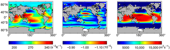
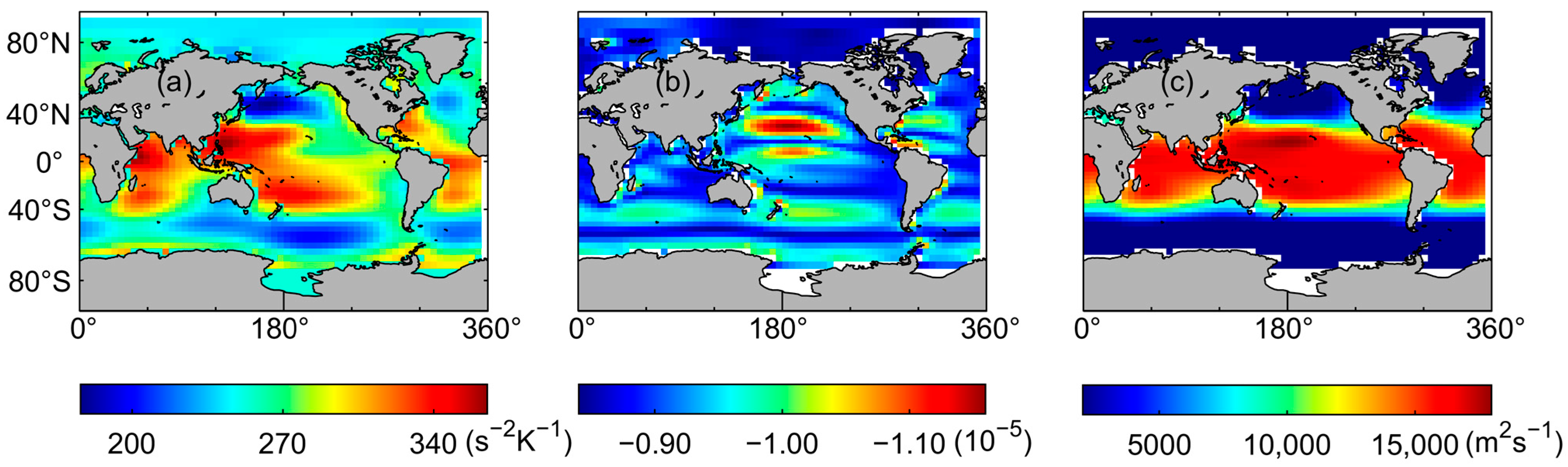
All three coupled components utilize a 64 (longitude) × 54 (latitude) Gaussian grid network and employ a leapfrog time-stepping scheme with the step size of half an hour. Further details about the coupled model can be found in the work of Wu et al. [13], including default parameter values. As this study focuses on geographical-dependent CPO, it is necessary to replace the globally uniform default values of certain parameters in the coupled model with parameter fields that exhibit geographic characteristics. As a basis, the ranges of , , and have been determined (see Table 1) by Cao et al. [1] through climatological simulation of this coupled model. Using the geographic distribution of the model states related to , , and , respectively, as a reference, we obtain the geographic distribution of the three parameters as shown in Figure 2. As such, the fields of , , and , instead of their globally uniform default values, will be utilized in the “true” model. And other parameters in the “true” model remain consistent with default values. The values of all parameters in the “true” model are noted as , and the “true” model is used to produce “observations”.
Table 1.
Ranges and default values of , , and under investigation.
Figure 2.
The geographic distribution of (a) , (b) , and (c) in the “true” model.
4. Numerical Experiments
4.1. Design of “Twin” Experiment
The success of parameter optimization is closely related to parameter sensitivity [12,17,42,43]. Cao et al. [1] conducted a systematical analysis of the coupled model used in this study based on instantaneous parameter sensitivity, which indicates that is the most sensitive parameter for oceanic streamfunction and is the most sensitive parameter for atmospheric streamfunction , and demonstrates that assimilation of observations of or could provide effective estimation of or . Note that is a weakly coupled coefficient, serving as an internal parameter of the ocean model, whereas is a strongly coupled coefficient which links the components between the atmospheric and oceanic (terrestrial) models. Values of over ocean grid points have geographic dependence, but over land grid points are fixed at the default value.
The previous study [35] on the coupled parameter optimization using A-4DEnVar has only been validated based on an idealized 1D coupled model. Since this paper presents an improvement to A-4DEnVar, it is necessary to conduct validation experiments under a WCDA framework firstly to assess the performance of the improved A-4DEnVar in this idealized 2D coupled model. Thus, we first conducted auxiliary validation experiments on parameter optimization of , where is optimized using only the observations of . This forms an important basis for presenting the coupled parameter optimization under SCDA framework in our study. Then, to evaluate the effectiveness of A-4DEnVar and DIP scheme in GPO, particularly in strongly coupled parameter optimization, is selected for optimization by assimilating observations of . And we only focus on optimizing upon the ocean since upon the land does not have geographic distribution.
The initial guess of or is set to globally default value (i.e., 253 s−2K−1 for and −1.00 × 10⁻⁵ for ). The “true” initial conditions are obtained by running the coupled model with for 50 years, starting from the climate state field , which includes the atmospheric streamfunction , the oceanic streamfunction , and the global surface temperature . Observations are sampled from the “true” model with intervals of 6 model hours (12 time steps) for and 24 model hours (48 time steps) for at all model grid points, without adding any noise.
4.2. Generation of the Ensemble Perturbation
As discussed in Section 2.2, although the improved A-4DEnVar imposes more stringent requirements on the independence of ensemble perturbation members and still necessitates that , the introduction of the independent point scheme relaxes this constraint. Specifically, it only requires , where , thereby enabling significant dimensionality reduction. In this subsection, a simple and efficient method is presented to generate an ensemble of perturbations with improved independence: for the parameters that need to be optimized at IPs, we traverse them serially, applying random perturbations only to the current IP while keeping all others unperturbed. This approach ensures that there is no covariance of parameter perturbations between different IPs within the current ensemble member. The ensemble, including samples of parameter perturbations, is generated exactly in the way that correctly spans the reduced dimension of the parameter space. Consequently, the dimension of (defined in Section 2.1) is (or expressed as ).
4.3. Geographic-Dependent Coupled Parameter Optimization
We firstly carry out two cases of weakly coupled parameter optimization experiments to validate the performance of single parameter optimization (SPO) in EXPV1 and the geographic-dependent optimization at all model grid points (GPO) in EXPV2 for under WCDA framework. Then, a total of 10 cases of strongly coupled parameter optimization experiments are conducted (see Table 2) in order to examine the performance of single-value parameter optimization (SPO) in EXP1, geographic-dependent optimization (GPO) of the parameters at all model grid points in EXP2, GPO with static independent point scheme (GPO-SIP) in EXP3~EXP6, and GPO with dynamic independent point scheme (GPO-DIP) in EXP7~EXP10 for under SCDA framework are conducted. In each experiment, only the targeted parameter (either or ) was assigned an incorrect initial value (i.e., contained a bias), while all other model settings and parameters remained identical to those of the “true” model.
Table 2.
Summary of settings for strongly coupled parameter optimization experiments.
It should be noted that EXPV2 and EXP2 are presented as conceptual, idealized benchmarks. They represent a full global parameter optimization (without introducing independent point scheme). In these two cases, . They are feasible only in our intermediate scale idealized model. Their purpose is to establish a theoretical performance upper bound and to validate the core optimization framework, providing a reference for evaluating the more practical geographic-dependent schemes (GPO-SIP and GPO-DIP). In practical, large-scale applications with grid points, such a global approach is computationally prohibitive.
The absolute value of the parameter perturbation is set to 1% of the overall average value of the first guess of the parameters to be optimized (i.e., 2.53 s−2K−1 for , and 1.00 × 10⁻⁷ for ). The scaling factor introduced by Equation (11), , is set to 10−6. In all experiments, five outer loops, each with 15 inner loops, are included, and the assimilation time window is set to 7 model days. The global root-mean-square error (RMSE), calculated between the simulated state variables and the corresponding “true” state fields, is used to quantify the effectiveness of the parameter optimization.
4.3.1. Performance of Single-Value Parameter Optimization
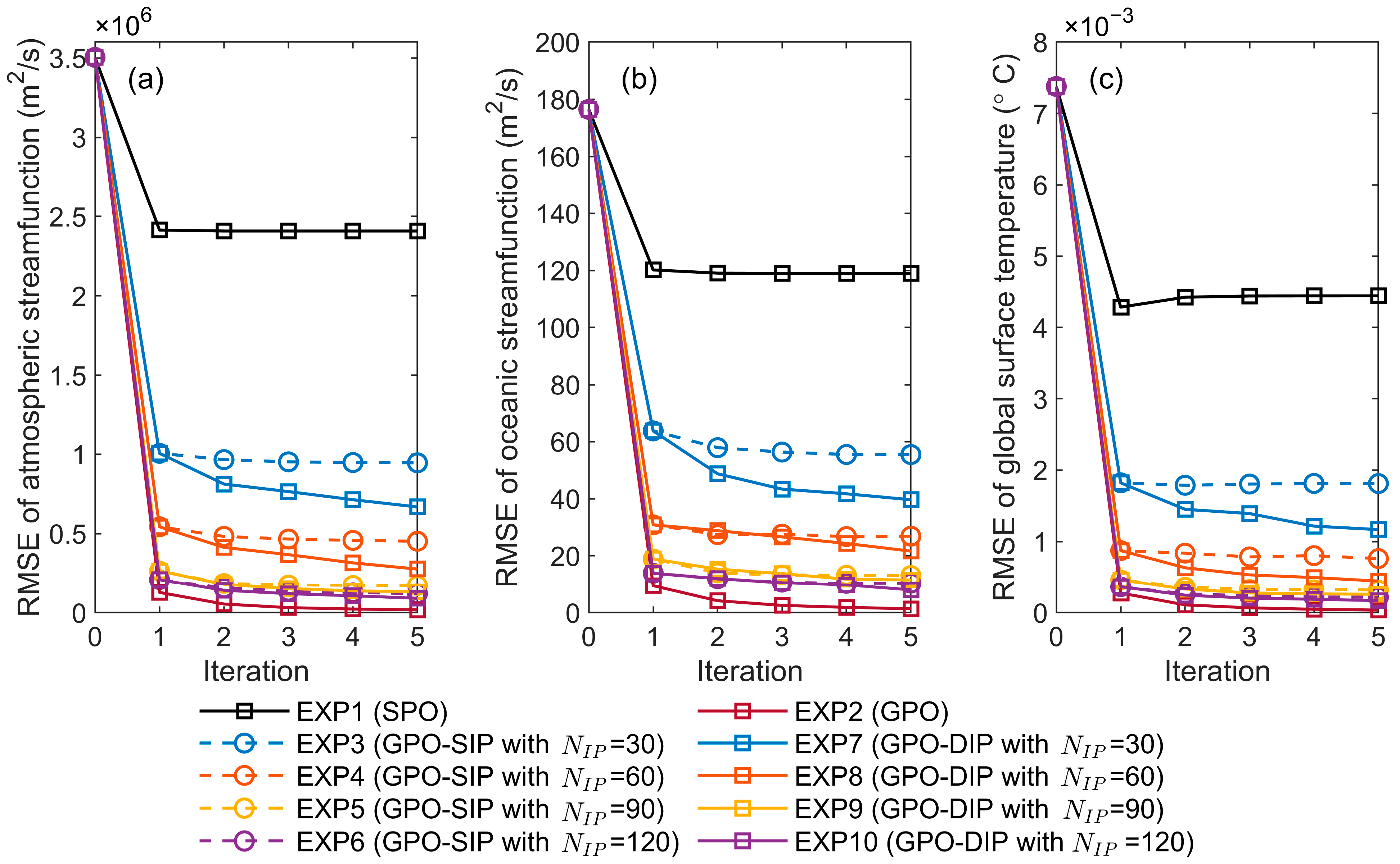
To investigate the performance of SPO, we assume that and are globally uniform with no geographic distribution in EXPV1 and EXP1, respectively. Firstly, we conduct the optimization of (EXPV1) to validate the performance of SPO using improved A-4DEnVar under the WCDA framework. After parameter optimization in EXPV1, the RMSEs for , , and decrease by 65.78%, 40.10%, and 41.53%, respectively. The global mean error of the optimized decreases to 4.62 × 10⁻⁷, compared to that of the first guess of (8.43 × 10⁻⁷). These results of EXPV1 indicate that A-4DEnVar can perform SPO under WCDA framework, even when the “truth” parameters are geographic-dependent. With this foundation, we further conduct SPO of (EXP1) under the SCDA framework. The RMSEs of , , and during the outer loops are shown by the black lines in Figure 9. It is clear that there is a significant decrease in RMSEs for all three state variables at the end of the first outer iteration, while subsequent iterations show little change, indicating that stability has been reached. After parameter optimization, the RMSEs for , , and decrease by 31.27%, 32.60%, and 39.78%, respectively. However, the global mean error of the optimized increases to 48.24 s−2K−1, compared to that of the first guess of (32.27 s−2K−1). Since SPO is a global averaging approach, it can reduce the RMSEs of state variables but fails to effectively represent the geographic distribution of . All observations are used to estimate a single value for , leading to a cancelation of parameter adjustments across different geographic regions and insufficient consideration of geographic dependence of .
4.3.2. Performance of Geographic-Dependent Parameter Optimization
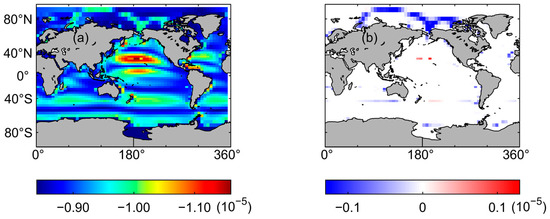
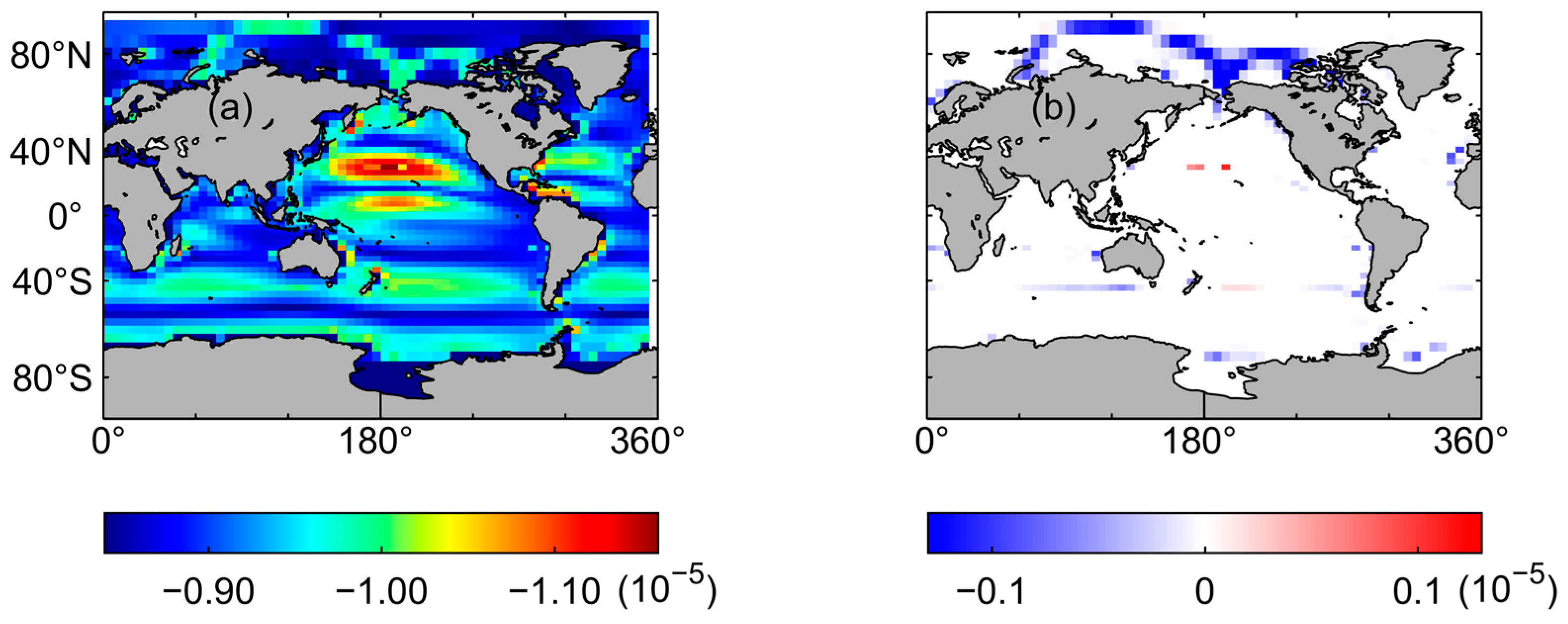
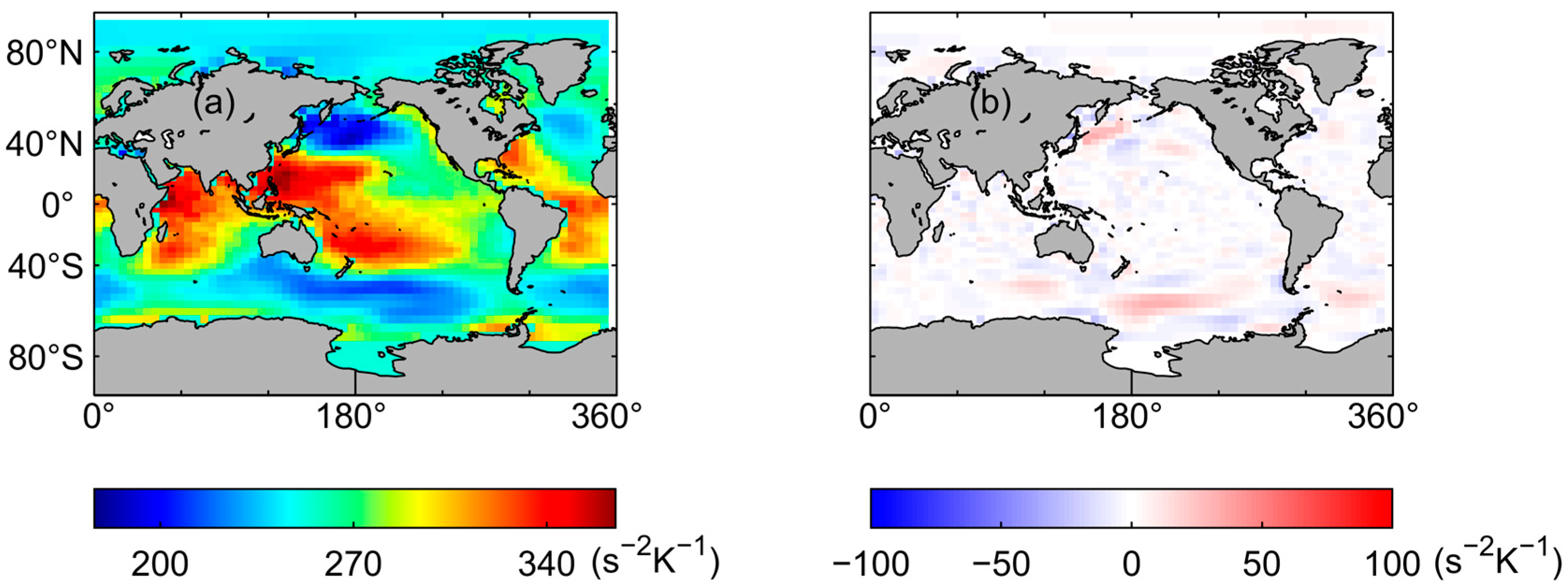
To examine the performance of GPO, we assume that or has geographic distribution at all the model grid points, and is allowed to be adjusted geographically during the optimization process. We also first conduct optimization of (EXPV2) to validate the performance of GPO using improved A-4DEnVar under the WCDA framework. The spatial distribution of the optimized in EXPV2 is plotted by Figure 3a. Its difference regarding the “truth” of is shown in Figure 3b. The optimized closely resemble the in the “true” model, effectively reflecting the geographic-dependent characteristics of parameters. After optimizing in EXPV2, the RMSEs for , , and decrease by 99.45%, 99.77%, and 98.36%, respectively. The results of EXPV2 validate that A-4DEnVar can successfully perform SPO under the WCDA framework. Based on this, we further conduct GPO of (EXP2) under the SCDA framework, which is one of the main focuses of this study. From the deep red lines with respect to EXP2 in Figure 9, the RMSEs for , , and after optimizing under decrease by 99.50%, 99.22%, and 99.50%, respectively. Figure 4 indicates the optimized in EXP2 possesses geographic-dependent characteristics almost identical to the “truth” of in Figure 2a, with very little difference. These results demonstrate that the improved A-4DEnVar can effectively capture geographic-dependent characteristics during the CPO, overcoming the strong nonlinear interference of the coupled model and exhibiting excellent data assimilation performance not only in the case of WCDA but also in the case of SCDA.
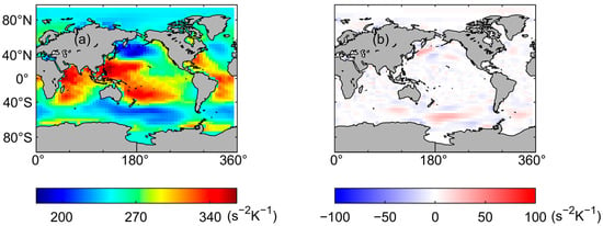
Figure 3.
Spatial distributions of (a) the optimized in GPO (EXPV2), and (b) its difference relative to the in the “true” model as shown in Figure 2b.
Figure 4.
Spatial distributions of (a) the optimized in GPO (EXP2), and (b) its difference relative to the in the “true” model as shown in Figure 2a.
4.3.3. Impact of Dynamic Independent Point Scheme in GPO
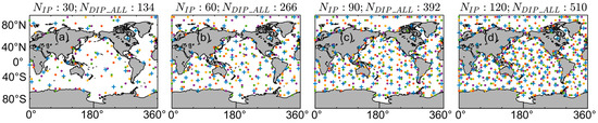
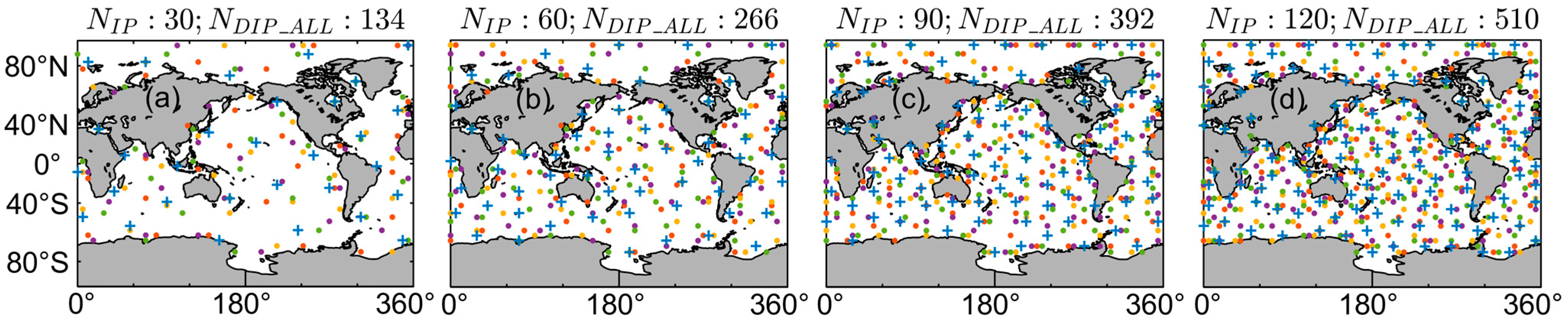
The superior performance of the improved A-4DEnVar in geographic-dependent optimization of the parameter under the WCDA and SCDA frameworks has been fully validated by EXPV2 and EXP2. However, the computational cost for parameter optimization across all model grid points is enormous, making it an impractical choice for high-dimensional models. Therefore, we further investigate and compare the impact of independent point schemes in reducing the computational cost and effectively capturing the geographic-dependent characteristics of parameter in GPO. Considering that this study focuses on the effectiveness of strongly coupled parameter optimization, all subsequent experiments are conducted under the SCDA framework for the optimization of . We discuss the optimization of with four cases where . Given that the outer loops include five iterations, each experiment using DIP scheme requires the selection of five sets of Ips, as outlined in Section 2.2. To enhance the comparison of GPO, the IPs selected in SIP scheme are consistent with the first set of IPs chosen in the DIP scheme for each case of . Here, we present the locations of IPs for these experiments using the DIP scheme in Figure 5. To show the aggregation of IPs across all iterations for each case, IPs in each set are color-coded. The number of all unique IPs across the five iterations is denoted as , which is roughly equal to the number of outer iterations (i.e., ) times , differing only by the number of repeated points. Thus, to distinguish it from , can be regarded as an indicator of the extent to which the DIP scheme explores the parameter space across all outer iterations during data assimilation. The larger indicates that more parameters are directly optimized during the data assimilation, effectively addressing the issue of non-selected grid points potentially providing critical information and reverse projection errors in non-independent grid points. But it still needs to be distinguished from . In Figure 5, the first set of IPs in DIP scheme which are also selected in SIP scheme marked as big blue plus signs, while the remaining IPs marked as small dots.
Figure 5.
Locations of the independent points for : (a) , (b) , (c) , and (d) . For DIP scheme, IPs of each set are used in each outer iteration. To ensure visual clarity, IPs in each set are color-coded. The first set of IPs, which is also selected in SIP scheme marked as big blue plus signs, while the remaining IPs marked as small dots.
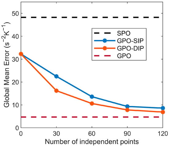
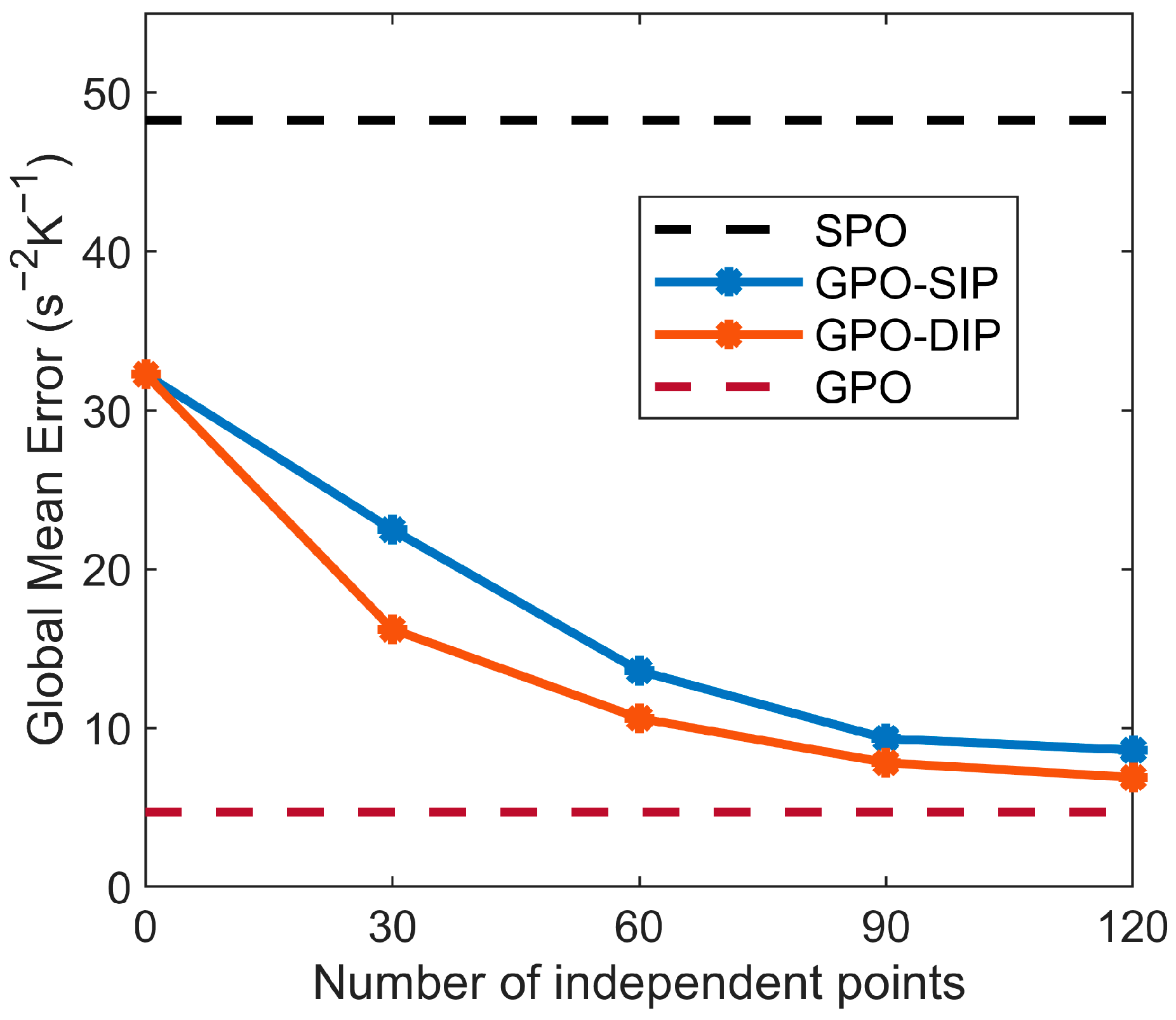
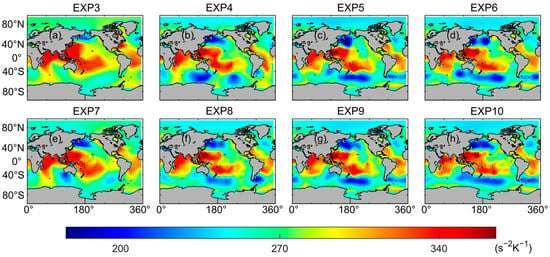
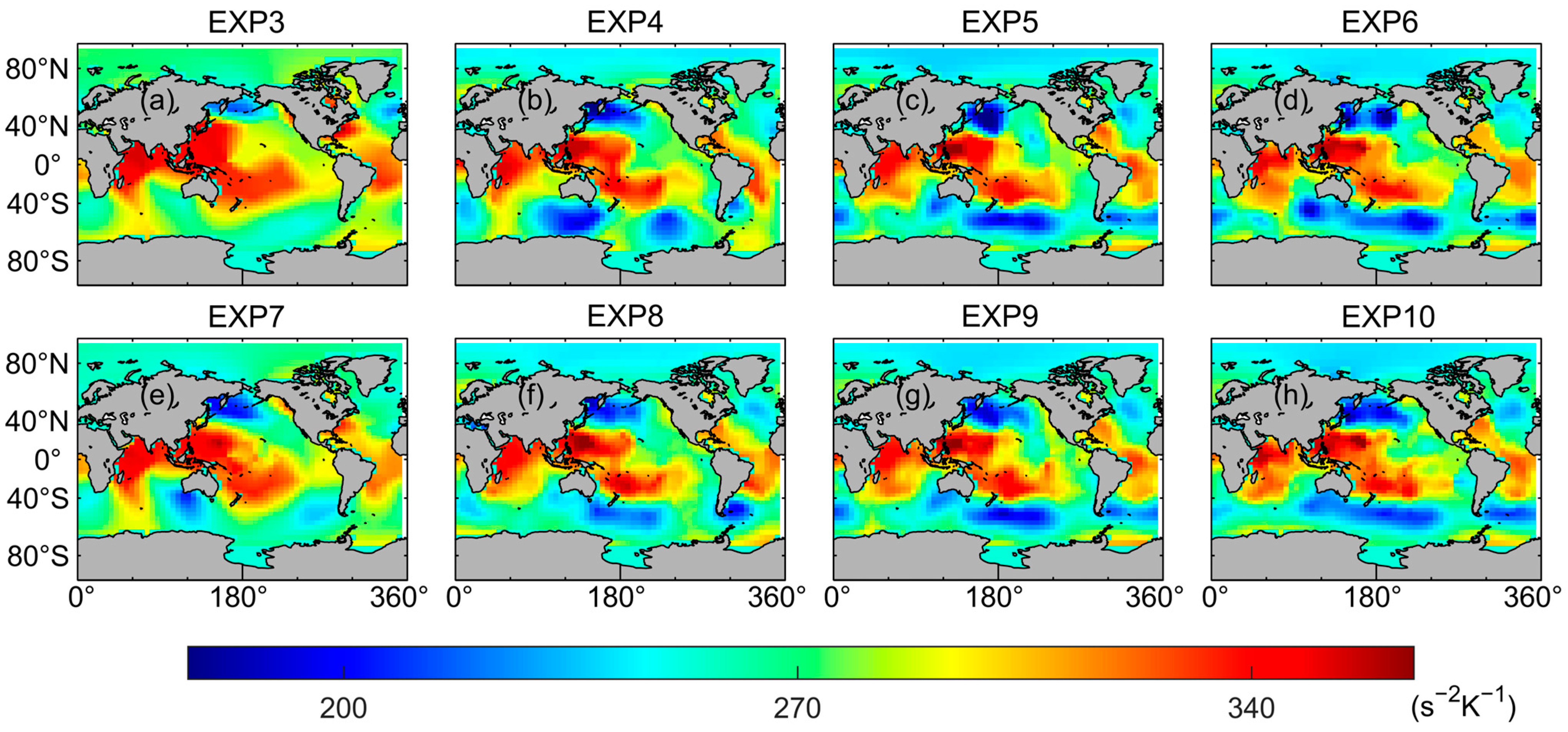
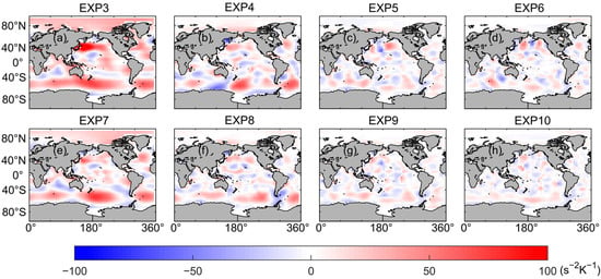
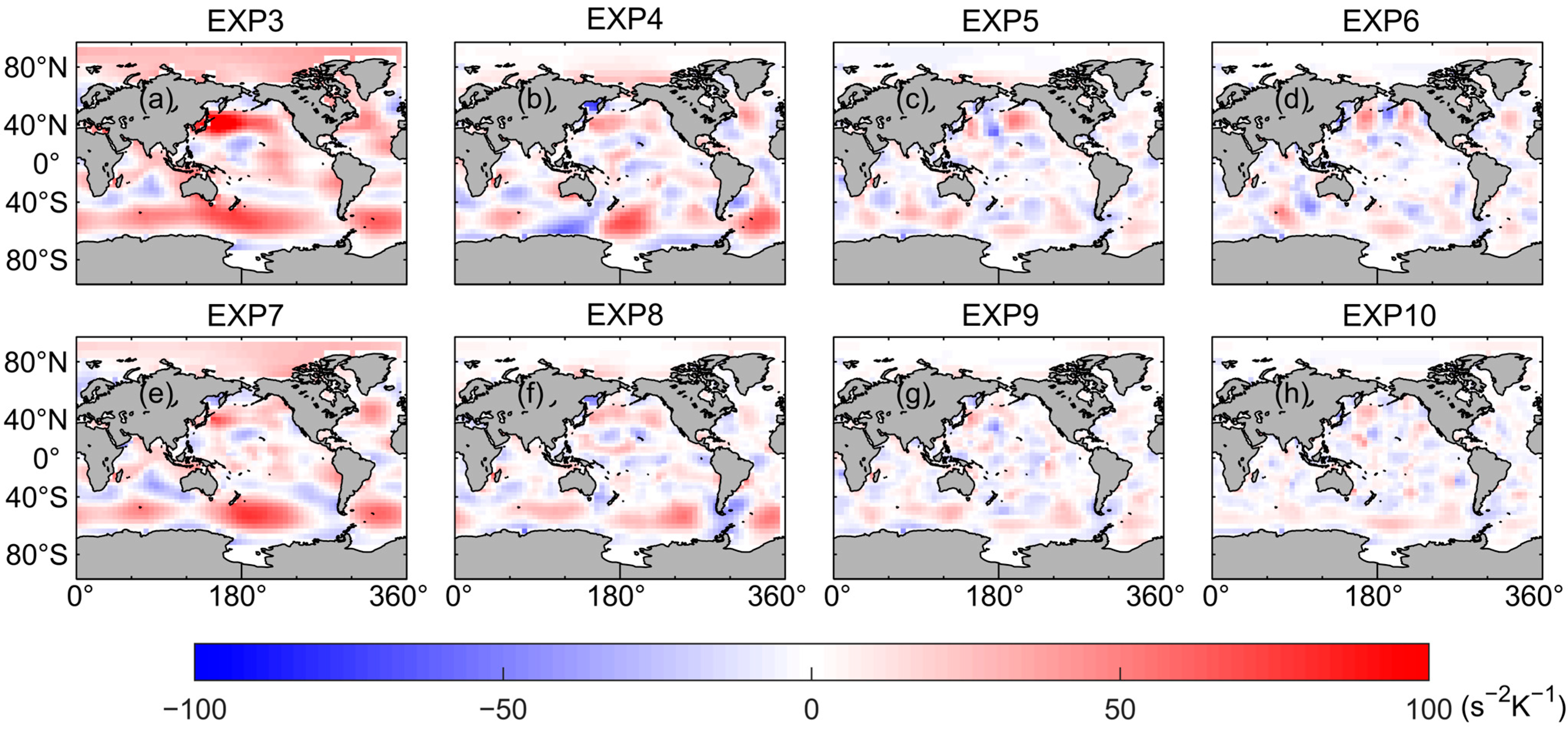
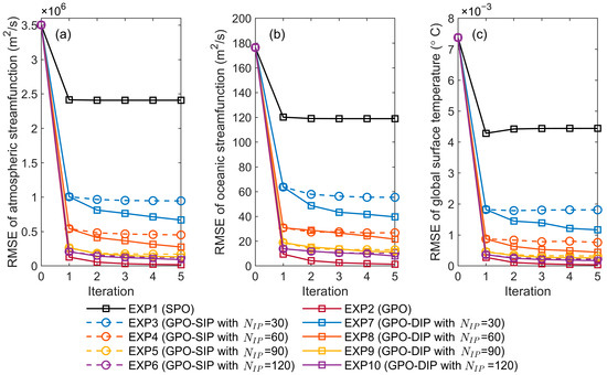
From Figure 6, for both GPO-SIP and GPO-DIP, more IPs can further reduce the global average error of the optimized , leading to the parameter distribution closer to the “true” model (Figure 7) and enhancing the effectiveness of GPO. For the same , GPO-DIP yields a smaller global average error of the optimized compared to GPO-SIP (Figure 8). Upon the completion of parameter optimization, the RMSEs for , , and in GPO-DIP are significantly lower than that in GPO-SIP. And after just the second outer-loop in GPO-DIP, the RMSEs of shown in Figure 9a and shown in Figure 9c are even lower than those produced by GPO-SIP after all outer-loop iterations. Furthermore, the RMSEs of in GPO-SIP stabilizes after the third outer-loop, while the DIP scheme continues to expand the dimensionality of the parameter subspace with each additional outer loop iteration, leading to superior performance of GPO. Both Figure 6 and Figure 9 illustrate that as decreases, the advantages of the DIP scheme become more pronounced. This can be regarded as the effective compensation for the poorer performance with smaller in GPO-SIP. Therefore, when selecting an independent point scheme, whether due to computational resource limitations that necessitate fewer outer loop iterations or the desire to pursue optimal parameter optimization effectiveness, the DIP scheme is the superior choice.
Figure 6.
Impact of the number of independent points on global mean errors of the optimized . The case with zero independent points (far left) corresponds to the result without data assimilation (i.e., using the first guess of ). The black and red horizontal dashed lines indicate the global mean errors of the optimized in SPO (EXP1) and GPO (EXP2), respectively.
Figure 7.
Spatial distributions of optimized in (a–d) GPO-SIP and in (e–h) GPO-DIP.
Figure 8.
Spatial distributions of the difference of the optimized in (a–d) GPO-SIP and in (e–h) GPO-DIP relative to the “true” .
Figure 9.
RMSEs of (a) , (b) , and (c) decrease with outer iterations.
This subsection demonstrates that the introduction of the independent point scheme, particularly the DIP scheme, in the A-4DEnVar framework significantly decreases the computational cost while effectively capturing the geographic-dependent characteristics of parameters. In practical applications, the number of independent points and the number of outer-loop iterations can be adjusted based on target accuracy requirements and computational resource limitations, which is crucial for operational applications.
It also shows strong performance not only in the WCDA but also in the SCDA. The results of the parameter optimization for in the paper clearly lead to the conclusion that optimizing the cross-component parameter can significantly improve the estimation accuracy of the state variables of different components in a coupled model. This has important implications for improving state estimation within the SCDA framework, suggesting that one must carefully optimize model parameters when aiming to further improve state estimation. Although this idea may be not new, as Cao et al. [1] has proposed similar insights within the scope of ensemble-based data assimilation, we are the first to validate this idea in GPO through variational methods, thus expanding the application of SCDA, particularly for CPO.
4.4. Impact of Coupled Parameter Optimization on “Climate Prediction”
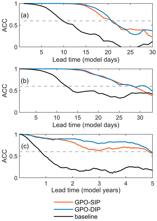
The previous work has demonstrated the excellent performance of A-4DEnVar in geographic-dependent coupled parameter optimization, which effectively reduces model bias, particularly with the introduction of the DIP scheme. However, it remains necessary to investigate the impact of the optimized parameters on “climate prediction” of the coupled model. Given that A-4DEnVar relies on model performance within the data assimilation time window, the longer time window in long-term forecasting (noting that different state variables exhibit distinct predictable temporal scales, and thus correspond to different “long-term forecasts” defined relative to their respective scales, which will be critical for subsequent discussions) may lead to the accumulation of model biases, including parameter errors, potentially resulting in degraded performance of model simulations and predictions. To further evaluate the performance of the proposed scheme in “climate prediction”, we conduct three types of forecast experiments: (1) the “forecast tests”, which use the optimized from EXP5 (GPO-SIP with ) and EXP7 (GPO-DIP with ); (2) the “baseline tests”, which use the first guess of ; (3) the “true tests”, which use the in the “true” model. All other experiment settings are kept consistent with , and the initial conditions for these experiments are identical to the “true” initial conditions obtained in Section 4.1. The anomaly correlation coefficient (ACC), as one of the most widely used measures in evaluating the forecast skill, is utilized to evaluate the forecast tests and the “baseline” tests. ACC is calculated between the forecast anomaly field and the verifying analysis (or truth) anomaly field. Note that an ad hoc value of 0.6 of ACC is used here to determine a lead time for a skillful forecast [44].
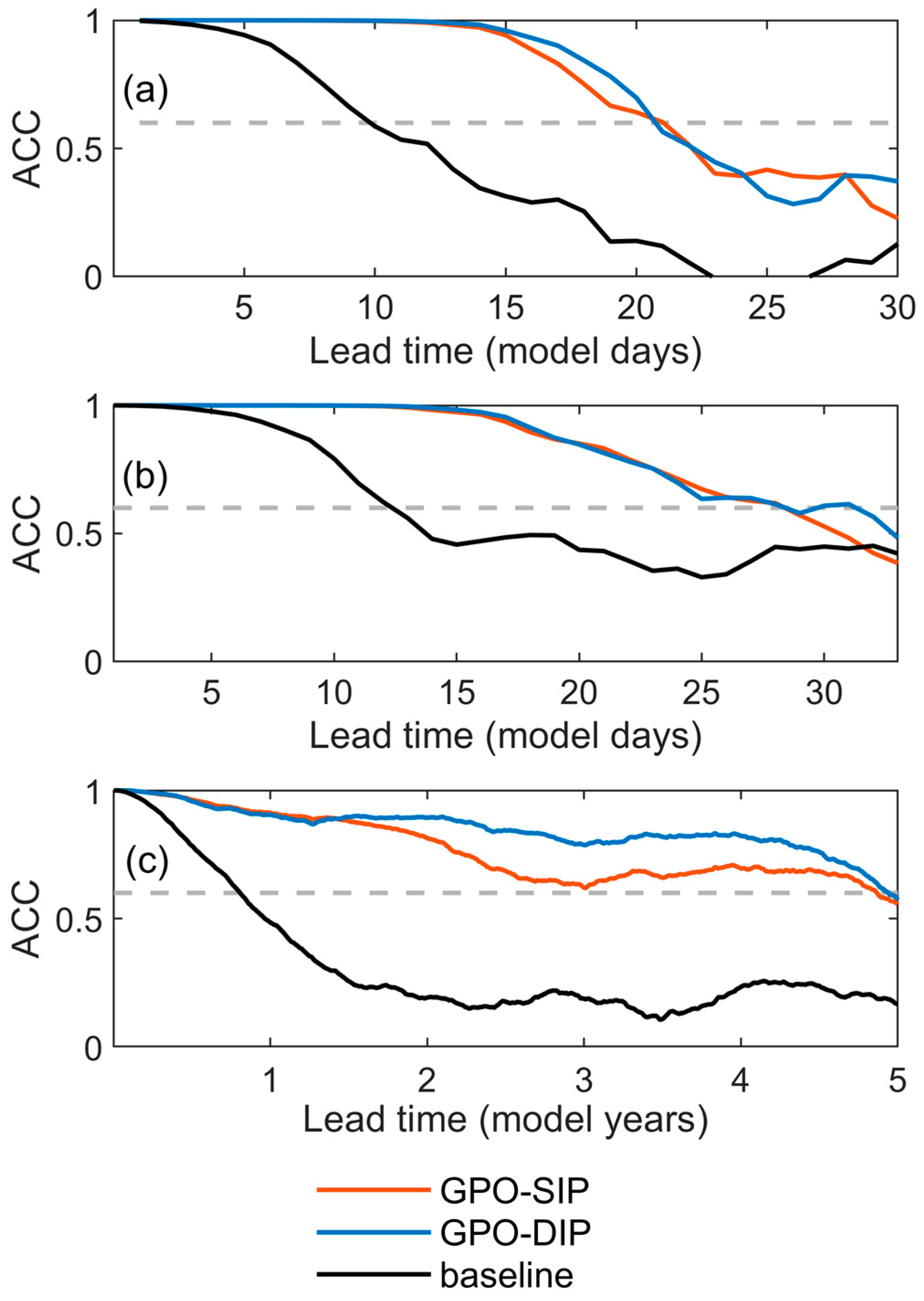
From the comparison with the results of ACC in the “baseline” tests in Figure 10, the geographic-dependent coupled parameter optimization based on A-4DEnVar plays an essential role in improving forecast skill. The absence of any abrupt decline or oscillation in the ACC at the initial forecast times confirms that the parameter optimization scheme does not introduce destabilizing “initial shocks” to the coupled model. Furthermore, it can be observed that the DIP scheme not only shows better performance than the SIP scheme in parameter optimization, but also demonstrates higher forecasting accuracy (for and ) and longer forecast lead time (for and ). By optimizing parameters at only 90 IPs in GPO-DIP, the valid forecast of is extended from 9 days to 21 days as shown in Figure 10a, indicating that, even for state variables with strong nonlinearity, the forecast lead-time significantly exceeds the assimilation time window. The valid forecast of and are extended from 12 days to approximately 30 days from Figure 10b and from 10 months to 5 years from Figure 10c, respectively. Moreover, the results shown in Figure 10a are consistent with the conclusions drawn by Cao et al. [1] based on ensemble filtering. Thus, this also validates the issue raised in the first paragraph of this section, confirming that the parameter optimization performance based on A-4DEnVar remains highly stable in “climate prediction” for different state variables across their respective scales in the idealized coupled model. The proposed scheme can not only be applied for reanalysis, but also provide a new perspective when a coupled general circulation model is used for climate estimation and prediction.
Figure 10.
ACC as a function of forecast lead-time regarding (a) , (b) , and (c) produced by the first guess of ,the optimized in GPO-SIP and GPO-DIP. The horizontal dashed gray line indicates the ACC threshold of 0.6 used to determine the skillful forecast lead time.
5. Discussion
Compared to single-component Earth system models (ESMs), coupled ESMs play an increasingly important role in climate prediction research. Under coupled data assimilation (CDA) framework, coupled parameter optimization (CPO) can reduce the biases in a coupled model and enhance its forecast skill. A-4DEnVar is one of the most cutting-edge hybrid data assimilation schemes, which well retains the nonlinear processing capabilities of 4D-Var but avoids the adjoint model. In response to the demands of operational applications, A-4DEnVar has been improved by introducing a sample-space variable replacement approach and incorporating a novel dynamic independent point (DIP) scheme.
A series of parameter optimization experiments are conducted using an intermediate atmosphere–ocean–land coupled model. Results show that under the strong nonlinear influence of the coupled model, A-4DEnVar exhibits satisfactory assimilation performance in CPO. Comparing the results of single-value parameter optimization (SPO) and geographic-dependent optimization (GPO), we find that the geographic characteristics of parameters in GPO are captured effectively, significantly enhancing the optimization. These findings validate the effectiveness of the geographic-dependent coupled parameter optimization scheme based on A-4DEnVar, overcoming the application bottleneck of only performing single-value parameter optimization. Meanwhile, we can find that optimizing the cross-component parameter can significantly improve the estimation accuracy of the state variables of different components in the coupled model, which is more innovative and promising. Furthermore, both GPO-SIP and GPO-DIP schemes show that more independent points can further reduce the global average error of the optimized parameters, enhancing the effectiveness of GPO. With the same number of independent points, GPO-DIP performs better than GPO-SIP not only in geographic-dependent coupled parameter optimization but also in climate simulations. The fewer the independent points, the better performance of GPO-DIP than GPO-SIP. Additionally, the computational cost (measured in CPU seconds) of GPO-DIP is slightly greater than GPO-SIP as shown in Table 2. This is due to the computation of interpolation weight for each outer loop in GPO-DIP.
The computational cost of dynamically regenerating interpolation weights, which scales with model resolution, is a key consideration for applying the DIP scheme to ultra-high-resolution networks. This challenge can be effectively mitigated by implementing localized weight calculations alongside parallel computing strategies. Such optimizations would preserve exploratory advantage of the DIP scheme while maintaining computational feasibility at very high resolutions. Furthermore, a promising direction for future development is the integration of artificial intelligence (AI) techniques to intelligently guide or enhance the DIP scheme, aiming to merge its physical consistency with improved adaptive learning capability.
While this study focuses on optimizing a single parameter, the design principle of the DIP scheme suggests its strong potential for more complex, multi-parameter optimization problems. A key advantage is that the DIP scheme does not require prior knowledge of parameter sensitivities. Instead, its dynamic, stochastic, and spatially expansive search strategy allows it to discover the influential regions for each parameter throughout the optimization process. This makes it robust for multi-parameter problems, as it does not rely on a fixed sampling geometry that may prove suboptimal for some parameters. The superior performance of the DIP over SIP in our single-parameter experiments stems from this fundamental advantage in exploration, which is directly applicable to the higher-dimensional and more challenging optimization problem involving multiple parameters with complex interdependencies.
Currently, we still face several challenges. In the actual scenario of coupled ESMs, model biases originate from the uncertainty of multiple parameters and their parameterization schemes. And the best climate state may well be achieved by compensating errors in different processes rather than by best simulating a certain physical process [19]. One example about our study is that, if we conduct more comprehensive GPO-DIP experiments, we should simultaneously consider the initial biases of multiple sensitive parameters. By conducting a series of tests with either simultaneous or step-by-step parameter optimization, we aim to develop the optimal multi-parameter optimization scheme, which will be explored in future work. Additionally, a further challenge may be that in more sophisticated modeling applications, there are parameters that could be tuned as “geographic-dependent”, but that would likely be incorrect since the geographic dependence might be dependent on other poorly represented physics or parameters elsewhere in the model. For this, we need to identify which parameters should be tuned and which should be improved through better formulation.
6. Conclusions
This study demonstrates that the improved A-4DEnVar is effective and efficient for geographic-dependent coupled parameter optimization within a nonlinear coupled model framework. GPO successfully captures the geographic features of parameters, yielding superior results to SPO. Regarding the dimensionality reduction strategy for parameter optimization, the DIP scheme enhances optimization and climate simulation performance by exploring a broader parameter subspace beyond static independent points, which is an improvement over the SIP scheme. In summary, this study on the geographic-dependent CPO with improved A-4DEnVar offers new perspectives and insights into parameter optimization within the framework of both 4D-Var and CDA, which, as supported by its robustness under more realistic observational conditions (Appendix A), is promisingly expected to be applied in reanalysis and climate prediction based on coupled ESMs in the future.
Author Contributions
Conceptualization, L.C., W.L. and K.L.; methodology, J.H., L.C., W.L. and G.Z.; software, J.H.; validation, J.H., Y.Z. and Y.T.; formal analysis, J.H.; resources, G.H. and Q.Z.; writing—original draft preparation, J.H.; visualization, J.H.; supervision, X.W., H.L. and H.W.; funding acquisition, W.L. and Q.Z. All authors have read and agreed to the published version of the manuscript.
Funding
This research was funded by and the National Natural Science Foundation (42376190 and 425B2042) and the National Key Research and Development Program (2023YFC3107800) of China.
Data Availability Statement
The raw data supporting the conclusions of this article will be made available by the authors on request.
Conflicts of Interest
The authors declare no conflicts of interest.
Appendix A. Supplementary Experiment with Noisy and Sparse Observations
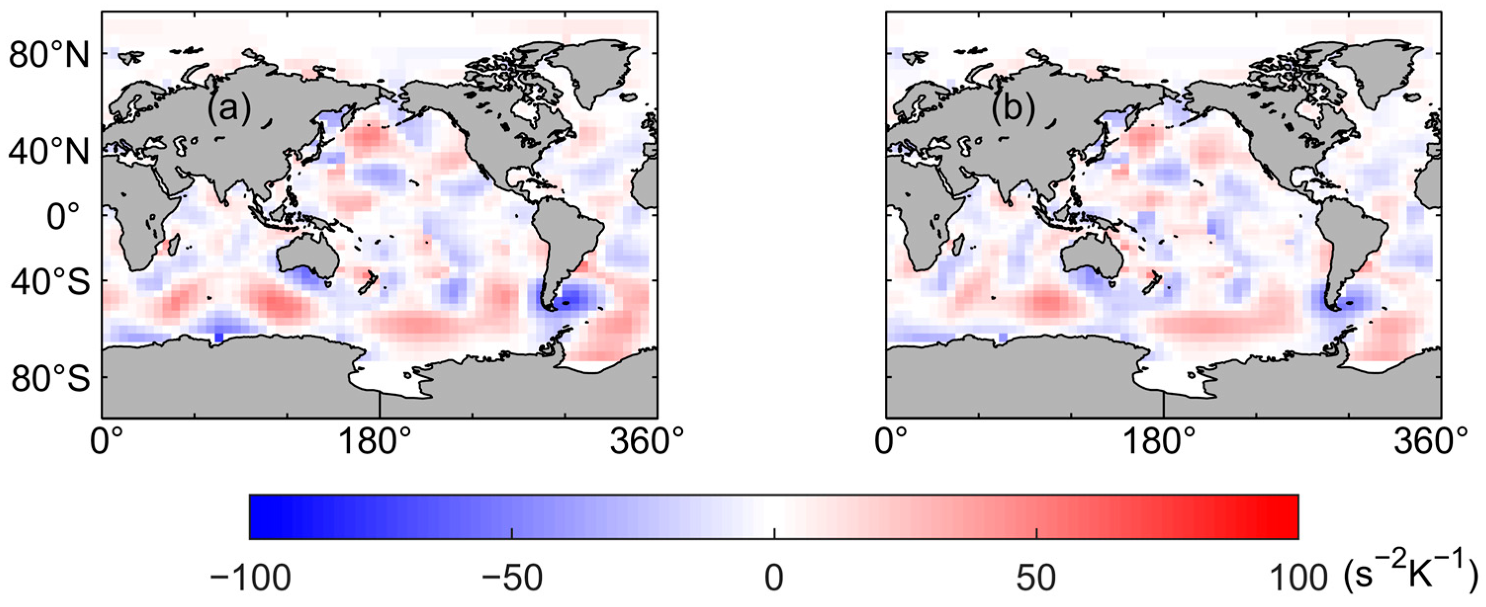
To assess robustness against realistic measurement errors, supplementary experiments were conducted under a more challenging observational setup. To move beyond the idealized “perfect twins” environment, the observational system was modified in two key ways. First, observations were made sparse by being present only at 90 IPs selected in the SIP scheme (or at the first set of 90 IPs in the DIP scheme), ensuring the number of observations is much smaller than the number of state variables. Second, observational white noise with an error level of 1% was added to these limited observations. This setup is more helpful in verifying the potential of this scheme for future application to realistic, complex coupled models.
From Figure A1 and Figure A2, it can be seen that even with very limited observations and the presence of observational noise, our scheme still demonstrates excellent performance. The optimized parameter distribution closely resembles optimized under perfect observations (full-grid observations without noise) and the “true” . For the additional experiment using the DIP method, the RMSEs for , , and T after optimizing decrease by 80.66%, 80.89%, and 81.86%, respectively. The global mean error of is 10.36 s−2K−1, which is only slightly higher than the 7.82 s−2K−1 attained under perfect observational conditions.
Figure A1.
Spatial distributions of the optimized in (a) GPO-SIP and in (b) GPO-DIP, using noisy and sparse observations.
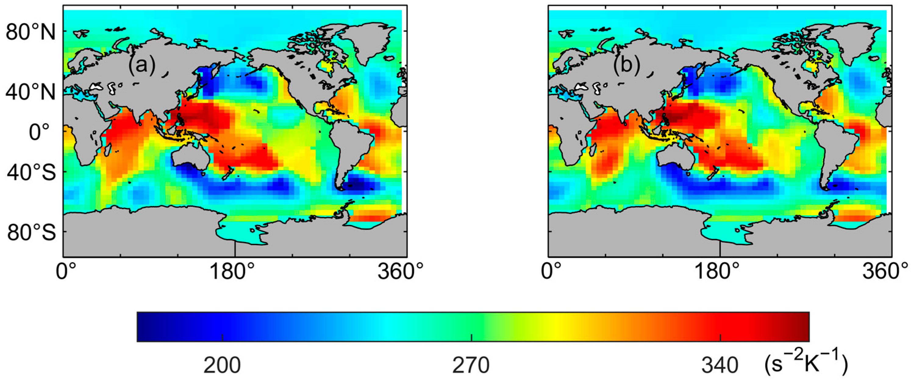
Figure A2.
Spatial distributions of the difference of the optimized in (a) GPO-SIP and in (b) GPO-DIP relative to the “true” , using noisy and sparse observations.
References
- Cao, L.G.; Han, G.J.; Li, W.; Wu, H.W.; Wu, X.B.; Zhou, G.F.; Zheng, Q.Y. Impact of Instantaneous Parameter Sensitivity on Ensemble-Based Parameter Estimation: Simulation with an Intermediate Coupled Model. J. Adv. Model. Earth Syst. 2024, 16, e2024MS004253. [Google Scholar] [CrossRef] [Scilit]
- Frolov, S.; Bishop, C.H.; Holt, T.; Cummings, J.; Kuhl, D. Facilitating Strongly Coupled Ocean-Atmosphere Data Assimilation with an Interface Solver. Mon. Weather Rev. 2016, 144, 3–20. [Google Scholar] [CrossRef] [Scilit]
- Laloyaux, P.; Balmaseda, M.; Dee, D.; Mogensen, K.; Janssen, P. A coupled data assimilation system for climate reanalysis. Q. J. R. Meteorol. Soc. 2016, 142, 65–78. [Google Scholar] [CrossRef] [Scilit]
- Lea, D.J.; Mirouze, I.; Martin, M.J.; King, R.R.; Hines, A.; Walters, D.; Thurlow, M. Assessing a New Coupled Data Assimilation System Based on the Met Office Coupled Atmosphere-Land-Ocean-Sea Ice Model. Mon. Weather Rev. 2015, 143, 4678–4694. [Google Scholar] [CrossRef] [Scilit]
- Penny, S.G.; Hamill, T.M. Coupled Data Assimilation for Integrated Earth System Analysis and Prediction. Bull. Am. Meteorol. Soc. 2017, 98, ES169–ES172. [Google Scholar] [CrossRef] [Scilit]
- Dee, D.P. Bias and data assimilation. Q. J. R. Meteorol. Soc. 2005, 131, 3323–3343. [Google Scholar] [CrossRef] [Scilit]
- Dee, D.P.; Da Silva, A.M. Data assimilation in the presence of forecast bias. Q. J. R. Meteorol. Soc. 1998, 124, 269–295. [Google Scholar] [CrossRef]
- Smith, D.M.; Cusack, S.; Colman, A.W.; Folland, C.K.; Harris, G.R.; Murphy, J.M. Improved surface temperature prediction for the coming decade from a global climate model. Science 2007, 317, 796–799. [Google Scholar] [CrossRef] [Scilit]
- Han, G.J.; Wu, X.R.; Zhang, S.Q.; Liu, Z.Y.; Navon, I.M.; Li, W. A Study of Coupling Parameter Estimation Implemented by 4D-Var and EnKF with a Simple Coupled System. Adv. Meteorol. 2015, 2015, 530764. [Google Scholar] [CrossRef] [Scilit]
- Zhang, S. A Study of Impacts of Coupled Model Initial Shocks and State Parameter Optimization on Climate Predictions Using a Simple Pycnocline Prediction Model. J. Clim. 2011, 24, 6210–6226. [Google Scholar] [CrossRef] [Scilit]
- Zhang, S. Impact of observation-optimized model parameters on decadal predictions: Simulation with a simple pycnocline prediction model. Geophys. Res. Lett. 2011, 38, L02702. [Google Scholar] [CrossRef] [Scilit]
- Zhang, S.; Liu, Z.; Rosati, A.; Delworth, T. A study of enhancive parameter correction with coupled data assimilation for climate estimation and prediction using a simple coupled model. Tellus Ser. A-Dyn. Meteorol. Oceanogr. 2012, 64, 10963. [Google Scholar] [CrossRef] [Scilit]
- Wu, X.R.; Zhang, S.Q.; Liu, Z.Y.; Rosati, A.; Delworth, T.L.; Liu, Y. Impact of Geographic-Dependent Parameter Optimization on Climate Estimation and Prediction: Simulation with an Intermediate Coupled Model. Mon. Weather Rev. 2012, 140, 3956–3971. [Google Scholar] [CrossRef] [Scilit]
- Wu, X.R.; Zhang, S.Q.; Liu, Z.Y.; Rosati, A.; Delworth, T.L. A study of impact of the geographic dependence of observing system on parameter estimation with an intermediate coupled model. Clim. Dyn. 2013, 40, 1789–1798. [Google Scholar] [CrossRef] [Scilit]
- Yan, C.; Zhu, J. A Simple Bias Correction Scheme in Ocean Data Assimilation. J. Mar. Sci. Eng. 2023, 11, 205. [Google Scholar] [CrossRef] [Scilit]
- Kitsios, V.; Sandery, P.; O’Kane, T.J.; Fiedler, R. Ensemble Kalman Filter Parameter Estimation of Ocean Optical Properties for Reduced Biases in a Coupled General Circulation Model. J. Adv. Model. Earth Syst. 2021, 13, e2020MS002252. [Google Scholar] [CrossRef] [Scilit]
- Tong, M.; Xue, M. Simultaneous Estimation of Microphysical Parameters and Atmospheric State with Simulated Radar Data and Ensemble Square Root Kalman Filter. Part II: Parameter Estimation Experiments. Mon. Weather Rev. 2008, 136, 1649–1668. [Google Scholar] [CrossRef] [Scilit]
- Hu, X.-M.; Zhang, F.; Nielsen-Gammon, J.W. Ensemble-based simultaneous state and parameter estimation for treatment of mesoscale model error: A real-data study. Geophys. Res. Lett. 2010, 37, L08802. [Google Scholar] [CrossRef] [Scilit]
- Schirber, S.; Klocke, D.; Pincus, R.; Quaas, J.; Anderson, J.L. Parameter estimation using data assimilation in an atmospheric general circulation model: From a perfect toward the real world. J. Adv. Model. Earth Syst. 2013, 5, 58–70. [Google Scholar] [CrossRef] [Scilit]
- Elbern, H.; Schmidt, H. Ozone episode analysis by four-dimensional variational chemistry data assimilation. J. Geophys. Res.-Atmos. 2001, 106, 3569–3590. [Google Scholar] [CrossRef] [Scilit]
- Rihan, F.A.; Collier, C.G.; Roulstone, I. Four-dimensional variational data assimilation for Doppler radar wind data. J. Comput. Appl. Math. 2005, 176, 15–34. [Google Scholar] [CrossRef] [Scilit]
- Wu, C.C.; Chou, K.H.; Wang, Y.Q.; Kuo, Y.H. Tropical cyclone initialization and prediction based on four-dimensional variational data assimilation. J. Atmos. Sci. 2006, 63, 2383–2395. [Google Scholar] [CrossRef] [Scilit]
- Chu, K.; Tan, Z.; Ming, X. Impact of 4DVAR assimilation of rainfall data on the simulation of mesoscale precipitation systems in a Mei-yu heavy rainfall event. Adv. Atmos. Sci. 2007, 24, 281–300. [Google Scholar] [CrossRef] [Scilit]
- Zhao, J.A.; Wang, B.; Liu, J.J. Impact of Analysis-Time Tuning on the Performance of the DRP-4DVar Approach. Adv. Atmos. Sci. 2011, 28, 207–216. [Google Scholar] [CrossRef] [Scilit]
- Gao, C.; Wu, X.R.; Zhang, R.H. Testing a four-dimensional variational data assimilation method using an improved intermediate coupled model for ENSO analysis and prediction. Adv. Atmos. Sci. 2016, 33, 875–888. [Google Scholar] [CrossRef] [Scilit]
- Kalnay, E.; Li, H.; Miyoshi, T.; Yang, S.-C.; Ballabrera-Poy, J. 4-D-Var or ensemble Kalman filter? Tellus Ser. A-Dyn. Meteorol. Oceanogr. 2007, 59, 758–773. [Google Scholar] [CrossRef] [Scilit]
- Lorenc, A.C. Recommended Nomenclature for EnVar Data Assimilation Methods; WGNE: Geneva, Switzerland, 2013; Volume 7. [Google Scholar]
- Liu, C.S.; Xiao, Q.N.; Wang, B. An ensemble-based four-dimensional variational data assimilation scheme. Part I: Technical formulation and preliminary test. Mon. Weather Rev. 2008, 136, 3363–3373. [Google Scholar] [CrossRef] [Scilit]
- Liu, C.S.; Xiao, Q.N.; Wang, B. An Ensemble-Based Four-Dimensional Variational Data Assimilation Scheme. Part II: Observing System Simulation Experiments with Advanced Research WRF (ARW). Mon. Weather Rev. 2009, 137, 1687–1704. [Google Scholar] [CrossRef] [Scilit]
- Buehner, M.; Houtekamer, P.L.; Charette, C.; Mitchell, H.L.; He, B. Intercomparison of Variational Data Assimilation and the Ensemble Kalman Filter for Global Deterministic NWP. Part I: Description and Single-Observation Experiments. Mon. Weather Rev. 2010, 138, 1550–1566. [Google Scholar] [CrossRef] [Scilit]
- Liu, C.S.; Xiao, Q.N. An Ensemble-Based Four-Dimensional Variational Data Assimilation Scheme. Part III: Antarctic Applications with Advanced Research WRF Using Real Data. Mon. Weather Rev. 2013, 141, 2721–2739. [Google Scholar] [CrossRef] [Scilit]
- Tian, X.J.; Feng, X.B. A non-linear least squares enhanced POD-4DVar algorithm for data assimilation. Tellus Ser. A-Dyn. Meteorol. Oceanogr. 2015, 67, 25340. [Google Scholar] [CrossRef] [Scilit]
- Liang, K.Z.; Li, W.; Han, G.J.; Shao, Q.; Zhang, X.F.; Zhang, L.; Jia, B.H.; Bai, Y.; Liu, S.Y.; Gong, Y.T. An Analytical Four-Dimensional Ensemble-Variational Data Assimilation Scheme. J. Adv. Model. Earth Syst. 2021, 13, e2020MS002314. [Google Scholar] [CrossRef] [Scilit]
- Liang, K.Z.; Li, W.; Han, G.J.; Wang, X.; Qiu, X.B. An operational improvement of A-4DEnVar and its application to the estimation of the spatially varying bottom friction coefficients of the M2 constituent in the Bohai and Yellow seas. Front. Mar. Sci. 2023, 9, 1084159. [Google Scholar] [CrossRef] [Scilit]
- Gong, Y.T.; Liang, K.Z.; Wu, X.R.; Shao, Q.; Li, W.; Liu, S.Y.; Han, G.J.; Liu, H.Y. An application of the A-4DEnVar to coupled parameter optimization. Acta Oceanol. Sin. 2022, 41, 60–70. [Google Scholar] [CrossRef] [Scilit]
- Anderson, J.L. An ensemble adjustment Kalman filter for data assimilation. Mon. Weather Rev. 2001, 129, 2884–2903. [Google Scholar] [CrossRef] [Scilit]
- Courtier, P.; Thépaut, J.-N.; Hollingsworth, A. A strategy for operational implementation of 4D-Var, using an incremental approach. Q. J. R. Meteorol. Soc. 1994, 120, 1367–1387. [Google Scholar] [CrossRef] [Scilit]
- Liu, D.C.; Nocedal, J. On the limited memory BFGS method for large scale optimization. Math. Program. 1989, 45, 503–528. [Google Scholar] [CrossRef] [Scilit]
- Cressman, G.P. An operational objective analysis system. Mon. Weather Rev. 1959, 87, 367–374. [Google Scholar] [CrossRef] [Scilit]
- Mu, M.; Zhou, F.; Wang, H. A Method for Identifying the Sensitive Areas in Targeted Observations for Tropical Cyclone Prediction: Conditional Nonlinear Optimal Perturbation. Mon. Weather Rev. 2009, 137, 1623–1639. [Google Scholar] [CrossRef] [Scilit]
- Liu, Z. Interannual positive feedbacks in a simple extratropical air–sea coupling system. J. Atmos. Sci. 1993, 50, 3022–3028. [Google Scholar] [CrossRef] [Scilit]
- Aksoy, A.; Zhang, F.; Nielsen-Gammon, J.W. Ensemble-based simultaneous state and parameter estimation with MM5. Geophys. Res. Lett. 2006, 33, L12801. [Google Scholar] [CrossRef] [Scilit]
- Tong, M.; Xue, M. Simultaneous Estimation of Microphysical Parameters and Atmospheric State with Simulated Radar Data and Ensemble Square Root Kalman Filter. Part I: Sensitivity Analysis and Parameter Identifiability. Mon. Weather Rev. 2008, 136, 1630–1648. [Google Scholar] [CrossRef] [Scilit]
- Hollingsworth, A.; Arpe, K.; Tiedtke, M.; Capaldo, M.; Savijärvi, H. The performance of a medium-range forecast model in winter–impact of physical parameterizations. Mon. Weather Rev. 1980, 108, 1736–1773. [Google Scholar] [CrossRef] [Scilit]

Disclaimer/Publisher’s Note: The statements, opinions and data contained in all publications are solely those of the individual author(s) and contributor(s) and not of MDPI and/or the editor(s). MDPI and/or the editor(s) disclaim responsibility for any injury to people or property resulting from any ideas, methods, instructions or products referred to in the content. |
© 2026 by the authors. Licensee MDPI, Basel, Switzerland. This article is an open access article distributed under the terms and conditions of the Creative Commons Attribution (CC BY) license.