


Abstract
This paper presents MeshVision, an open-source software tool for generating georeferenced, scaled, and textured 3D models of underwater environments from still images or video. Designed for non-expert users, MeshVision integrates video frame extraction, image enhancement, resizing, Structure-from-Motion reconstruction, dense reconstruction, texturing, orthomap generation, digital elevation modeling, and 3D measurement within a single workflow. The system also supports the integration of ROV navigation data for scaling and georeferencing. Evaluation across multiple deep-sea datasets acquired with different camera systems demonstrates the applicability of the workflow under varying environmental and acquisition conditions. The effect of fusion-based image enhancement on reconstructed geometry was quantitatively evaluated using three deep-sea datasets. Bidirectional surface-distance measurements and spatial-overlap analysis showed increases in triangulated mesh surface area ranging from 7.51% to 114.62%, accompanied by substantial dataset-dependent differences in geometric agreement. These comparisons characterize inter-model consistency and reconstructed surface extent rather than absolute geometric accuracy, as no independent ground-truth geometry was available. MeshVision additionally supports direct linear, angular, and strike-and-dip measurements on reconstructed scenes. Overall, the results demonstrate the utility of MeshVision as an accessible integrated framework for underwater 3D reconstruction, visualization, and quantitative analysis.
1. Introduction
Remotely Operated Vehicles (ROVs) and Autonomous Underwater Vehicles (AUVs) are widely used in oceanic research, providing an effective means to reach deep-sea locations and to capture high-quality still images and videos from previously inaccessible places [1,2]. The images and videos obtained can be incorporated into 2D photomosaics and textured 3D models, yielding rich data for a range of disciplines, including marine biology, geology, archaeology, and environmental monitoring. The textured 3D models provide a detailed representation of the three-dimensional spatial arrangement of seafloor features and thus support quantitative analyses of size, shape, and temporal change, especially in remote deep-sea areas where access to a site of interest may be limited to a single expedition. The ability to generate high-resolution 3D models also enables researchers to derive quantitative descriptors, such as rugosity, topographic complexity, feature distribution, and surface area, at multiple spatial scales, providing a richer three-dimensional basis for analysis than conventional 2D imagery alone. These metrics are critical indicators of habitat quality and biodiversity, especially in deep-water coral ecosystems and hydrothermally active areas or vent systems [3,4]. 3D photogrammetry enables temporal monitoring by allowing repeated measurements of the same area. This is particularly useful in assessing ecological dynamics, such as coral growth, mortality, or bleaching events.
Time-series and spatially extended photogrammetric surveys provide a non-destructive means to quantify morphological changes and evaluate the impact of anthropogenic disturbances or climate-related events [5]. In underwater archaeology, photogrammetry has become a standard tool for documentation, enabling the creation of georeferenced, scaled 3D models of shipwrecks, submerged settlements, and cultural artifacts. These models support both quantitative analysis, such as measuring object dimensions and spatial relationships, and qualitative interpretation by conservators and historians [6,7].
3D reconstruction methods, such as photogrammetry, provide a powerful means of converting 2D images or video footage into detailed 3D models of underwater scenes. These models capture the structure, size, and spatial relationships of underwater features. This is essential for interpreting complex underwater environments. The 3D reconstruction process typically involves image acquisition, feature extraction, matching, optimization, and the generation of a 3D point cloud or mesh. Consequently, the development of specialized software for underwater 3D reconstruction has become essential, enabling researchers and non-experts without programming backgrounds to convert large volumes of underwater image and video data into usable 3D models with minimal effort.
Recent developments in underwater photogrammetry have expanded the range of methods available for image-based three-dimensional reconstruction and quantitative habitat analysis. Zhong et al. [8] reviewed and compared conventional and emerging reconstruction approaches for underwater coral reef imagery, highlighting the challenges of reliable camera-pose estimation and dense reconstruction in underwater environments. Barrera-Falcón et al. [3] demonstrated the application of underwater photogrammetry to multiscale assessment of coral reef structural complexity, illustrating the potential of photogrammetric products for quantitative ecological analysis.
Several software tools have been developed for underwater 3D reconstruction, including Matisse and 3DMetrics [9], which provide important photogrammetric processing capabilities for underwater imagery. However, many existing workflows still require the combined use of separate applications or processing tools for frame extraction, image enhancement, reconstruction, visualization, and measurement. This increases processing complexity, especially for non-expert users. MeshVision does not introduce a new Structure-from-Motion or Multi-View Stereo algorithm. Instead, its contribution is the integration of underwater-image preprocessing, OpenMVG-based sparse reconstruction, OpenMVS-based dense reconstruction and texturing, navigation-data handling, geospatial product generation, visualization, and interactive measurement within a unified workflow for ROV-derived imagery. MeshVision additionally provides workflow-level functions for data preparation, reconstruction control, navigation association, generation of orthomaps and DEMs, and structural measurements directly on reconstructed scenes (Figure 1).
Figure 1.
Overview of MeshVision Software Version 2.0.
Table 1 summarizes the principal workflow-level similarities and differences between MeshVision and the Matisse and 3DMetrics software suite [9]. Both approaches use established open-source photogrammetric components and support underwater imagery and navigation data; the distinction of MeshVision lies primarily in integrating preprocessing, reconstruction, geospatial-product generation, visualization, and structural measurement within a single workflow, together with interactive angular and strike-and-dip measurement capabilities that are not explicitly reported in [9].
Table 1.
Workflow-level comparison of Matisse/3DMetrics and MeshVision. Entries for Matisse/3DMetrics are based on functionality reported in [9].
The main contributions of this work are:
- Integration of preprocessing, OpenMVG/OpenMVS reconstruction, visualization and analysis within one workflow;
- Support for underwater-image enhancement and video-derived datasets;
- Integration of ROV navigation information for scaling and georeferencing;
- Generation of orthomaps and DEMs from reconstructed scenes;
- Interactive distance, angle, and strike-and-dip measurements with persistent strike-and-dip measurement records;
- Evaluation on four real deep-sea ROV datasets acquired with different camera systems.
In addition to demonstrating the workflow across multiple deep-sea datasets, this study investigates the effect of underwater image enhancement on reconstructed geometry using three representative environments: Hydrothermal Chimney (PS119), Barnacle Crest (SO273), and Hydrothermal Field (MSM109). For each dataset, raw-image and fusion-enhanced reconstructions are compared in terms of reconstructed mesh surface area, bidirectional surface distances, and geometric agreement within commonly reconstructed spatial regions. Because the comparisons do not include independently measured reference geometry, they are intended to characterize the influence of preprocessing on reconstructed geometry rather than establish absolute reconstruction accuracy.
To demonstrate the applicability of the software tool, we present results on four underwater datasets acquired using four different camera systems (see Table 2). The datasets were acquired during four different expeditions using the deep-sea ROV Quest 4000, operated and developed at MARUM, University of Bremen. MeshVision is provided as an open-source software platform for underwater 3D reconstruction and quantitative analysis. The current release supports both Linux and Windows operating systems, and the source code, installation instructions, and user documentation are available at MARUM Cloud: https://cloud.marum.de/s/YeCGYn2TyM9BPXG (accessed on 11 June 2026). To support usability and reproducibility, a supplementary MeshVision Quick Start Guide accompanies this paper and provides a step-by-step workflow covering data import, preprocessing, reconstruction, orthomap and DEM generation, and interactive measurements.
Table 2.
Summary of the underwater datasets and corresponding stage-wise processing times obtained using standardized OpenMVG and OpenMVS reconstruction parameters on identical computing hardware. Camera-specific initialization parameters and image resolutions were retained according to the characteristics of each dataset. The principal reconstruction settings are provided in Supplementary Table S6.
The reconstruction experiments were performed on a workstation equipped with Intel Xeon E5-2623 v4 processors (Broadwell generation, 2.60 GHz) and approximately 128 GB of RAM. The OpenMVS logs reported 16 logical processors and a Linux 6.8.0-90-generic (x86_64 architecture) operating-system kernel. OpenMVG feature extraction was configured to use 16 threads, whereas OpenMVS used automatic thread selection. The maximum process virtual-memory allocations recorded across the available OpenMVS stages were 32.50 GiB for PS 119, 29.71 GiB for MSM 109, 28.60 GiB for SO 273, and 167.18 GiB for MSM 131. These values represent peak virtual address space rather than peak resident physical RAM. The execution logs did not provide continuous CPU or GPU utilization measurements, complete compilation settings, or dataset-specific storage footprints. Consequently, the reported stage-wise processing times should be interpreted as measurements under the documented experimental configurations rather than hardware-independent performance benchmarks.
2. Data Acquisition and Processing Workflow
Figure 2 summarizes the proposed workflow from data acquisition to textured 3D model generation. The pipeline accepts still images or video sequences as input and can additionally incorporate navigation data when available. This flexible design allows the workflow to be applied to a wide range of underwater survey configurations, including still-image camera systems, frame extraction from ROV video, and integrated telemetry and navigation data. As a result, the workflow is suitable for both image-only reconstruction and reconstructions that require scaling and georeferencing based on external navigation information.
Figure 2.
MeshVision 3D reconstruction pipeline.
During preprocessing, frames are extracted from the video, images are enhanced, resized, and filtered to reduce redundancy. These operations are designed to improve the quality and consistency of the input data before reconstruction. Frame extraction enables the use of standard video recordings as photogrammetric input. At the same time, image enhancement improves contrast and visibility under typical underwater conditions, which are affected by color attenuation, scattering, and low illumination. Resizing reduces computational demand, and redundant-image removal improves efficiency by limiting the number of highly similar images sent to the reconstruction stage. Together, these preprocessing steps improve both the practical usability of the workflow and the robustness of subsequent feature-based reconstruction.
Feature extraction and matching are then performed to establish correspondences between overlapping images. These correspondences form the basis for estimating camera poses and reconstructing the scene geometry. Once reliable image matches have been identified, sparse reconstruction is performed to recover the initial three-dimensional scene structure and the relative camera orientations. This is followed by dense point cloud generation, which increases the number of reconstructed surface points and provides a more complete geometric representation of the surveyed environment.
After densification, the workflow proceeds to mesh reconstruction and texture mapping. During meshing, the dense point cloud is converted into a continuous surface representation that approximates the scene’s morphology. Texture mapping then projects radiometric information, including pixel color and lighting, from the original images onto the reconstructed mesh, producing a visually coherent textured 3D model. This combination of geometric reconstruction and texture generation is important for underwater applications, where both surface shape and visual appearance contribute to geological, biological, and ecological interpretation.
When navigation data are available, they are associated with the corresponding images during preprocessing using acquisition timestamps. The ROV navigation records contain longitude, latitude, and depth together with their timestamps. Each image or video-extracted frame is time-matched to the corresponding navigation record, and the associated position and depth information are written into the image EXIF metadata before reconstruction. The geotagged images are subsequently passed to OpenMVG, where the embedded latitude, longitude, and depth information is used as positional prior information to support scaling and georeferencing. For the investigated reconstructions, OpenMVG was configured to use navigation-derived camera positions as positional priors (use_pose_prior = 1 and prior_usage = true), with a uniform configured weight of 1.0 for the three spatial coordinates. During bundle adjustment, these priors contribute weighted camera-centre residuals alongside image-reprojection residuals, while camera poses and intrinsic parameters remain adjustable. Thus, the navigation information acts as a soft positional constraint that supports metric scaling and georeferencing without rigidly fixing the resulting SfM solution.
This procedure maintains the association between individual images and the original ROV navigation data and enables reconstructed models to be placed within a spatial reference framework. Longitude, latitude, and depth are used for image geotagging and positional priors, while additional telemetry such as heading, pitch, roll, and altitude is retained for visualization and contextual interpretation. For geospatial output generation, geographic coordinates are transformed from WGS84 latitude and longitude to the corresponding UTM zone. ROV water depth is recorded as positive downward in the navigation data and represented as negative altitude/elevation in the georeferenced reconstruction and DEM outputs. The final outputs include textured 3D models that are ready for visualization, quantitative measurement, and further analysis. In addition, the workflow supports the generation of derivative products, such as orthomaps and digital elevation models, which enhance the analytical value of the reconstruction and further support spatial interpretation.
Overall, the MeshVision pipeline provides a practical workflow for underwater image-based 3D reconstruction by combining preprocessing, photogrammetric reconstruction, texturing, orthomap and DEM generation, and interactive measurement within a single software environment. This integration reduces the need to transfer data between separate tools and supports the analysis of ROV-derived image and video datasets by both non-expert and advanced users.
2.1. Image Acquisition
The quality of underwater photogrammetric reconstruction depends strongly on image-acquisition strategy, camera stability, and scene coverage [14]. In underwater environments, challenges such as limited visibility, uneven illumination, vehicle motion, and complex relief can reduce image quality and negatively affect feature matching [15]. For this reason, image acquisition must be planned to maximize overlap and to capture the scene from sufficiently diverse viewpoints for robust Structure-from-Motion (SfM) and Multi-View Stereo (MVS) processing.
Depending on the geometry of the surveyed target, different acquisition strategies may be appropriate. Parallel transects are commonly used for sub-horizontal seafloor areas, circular trajectories are suitable for localized free-standing objects, and spiral or hybrid paths are useful for vertically developed or morphologically complex structures. In practice, underwater surveys often combine these strategies to achieve adequate scene coverage while adapting to local terrain and operational constraints.
Regardless of the specific acquisition pattern, several general principles are critical for reliable reconstruction. Consecutive images should maintain high overlap, typically on the order of 70–90%, to ensure stable feature correspondences across views [16]. A combination of nadir and oblique perspectives can improve geometric coverage and reduce occlusions [17]. Camera settings should remain as consistent as possible throughout the survey to minimize frame-to-frame variability, and appropriate lighting should be used to reduce backscatter and improve feature visibility. When available, navigation data, scale bars, or other external references can further support scaling and georeferencing of the reconstructed scene [18].
In the context of MeshVision, these acquisition considerations are important because they directly influence the quality of the input data provided to the preprocessing and reconstruction pipeline. Well-planned image acquisition improves feature detectability, increases reconstruction completeness, and enhances the reliability of the textured 3D models and derivative products generated by the workflow.
2.2. Image Preprocessing
Image preprocessing is a critical first step in any 3D reconstruction pipeline, ensuring that input data are of sufficient quality and consistency to support reliable reconstruction. Before running algorithms such as Structure-from-Motion (SfM) or Multi-View Stereo (MVS), the images must be prepared to optimize performance, minimize computational complexity, and enhance feature detection reliability. The key preprocessing steps include image enhancement, resizing, and removing redundant images.
Image enhancement is particularly important for underwater imagery, which is often degraded by low contrast, color attenuation, scattering, and non-uniform illumination. These effects reduce the detectability of stable feature correspondences across views and can negatively affect both sparse and dense reconstruction. To address this problem, MeshVision integrates several underwater image enhancement methods prior to reconstruction. Among these, two representative methods are illustrated in Figure 3. The first is a dark-channel-prior-based dehazing method, which estimates transmission from a single degraded image and restores visibility and contrast [19]. The second is a fusion-based enhancement method, which combines color-corrected and contrast-enhanced inputs in a multiscale fusion framework to improve overall visual quality [20].
Figure 3.
Comparison of representative image enhancement techniques during the MeshVision preprocessing stage: (a) Raw underwater image. (b) Dark-channel-prior-based dehazing (DCPD) method. (c) Fusion-based enhancement (FE) method.
In addition to enhancement, MeshVision supports image resizing to reduce computational demand when processing high-resolution datasets. While larger images may preserve finer visual details, they also increase memory usage and processing time. Resizing therefore provides a practical trade-off between reconstruction detail and computational efficiency. The workflow also includes redundant-image removal, which is particularly useful for video-derived datasets with very high frame overlap. Removing highly similar images reduces unnecessary matching operations and improves overall processing efficiency. During image enhancement and resizing, the original EXIF metadata, including the associated navigation information, are preserved in the processed output images so that identical positional priors remain available for subsequent reconstruction.
Together, these preprocessing steps improve both the quality of the input imagery and the practical usability of the reconstruction pipeline. Figure 3 illustrates the visual effect of the two enhancement methods by comparing the raw input image with its enhanced counterparts.
2.3. Effect of Image Enhancement on Reconstructed Geometry
Underwater image acquisition is frequently affected by low contrast, color attenuation, and light scattering, which can reduce feature matching and influence Structure-from-Motion (SfM) and Multi-View Stereo (MVS) reconstruction. To investigate the influence of image enhancement on reconstructed geometry, three representative deep-sea datasets were evaluated: Hydrothermal Chimney, Barnacle Crest, and Hydrothermal Field.
For each dataset, two independent 3D reconstructions were generated using MeshVision: one from the original images and another from images processed using the fusion-based enhancement (FE) method illustrated in Figure 3c. The raw-image and enhanced-image reconstructions were generated independently using corresponding image sets and consistent reconstruction settings within each dataset.
The resulting meshes were registered in MeshLab Version 2020.09 [21] to establish a common coordinate frame for geometric comparison. Registration involved rigid transformations comprising rotation and translation, without additional uniform scaling in the final comparisons. The registration transformations were taken into account when calculating surface areas and geometric discrepancies.
The raw-image reconstruction served as a comparison surface rather than independently measured ground truth. Consequently, the experiments quantify inter-model differences and reconstructed mesh extent rather than absolute geometric accuracy.
2.3.1. Bidirectional Surface-Distance Evaluation
Geometric differences were evaluated using bidirectional unsigned surface-distance measurements. Points sampled from the FE reconstruction were compared with the closest surface points on the raw-image reconstruction (FE-to-raw), and the calculation was repeated in the reverse direction (raw-to-FE).
The MeshLab face-sampling method was applied using a standardized sampling density of approximately 100,000 points per square metre of triangulated mesh surface. For each sampled point, the Euclidean distance to the closest point on the comparison mesh was determined. The distributions were characterized by the mean; root mean square (RMS); median; 90th (P90), 95th (P95), and 99th (P99) percentiles; and maximum sampled distance.
Additionally, the percentage of distances within 4 cm was calculated. This threshold was used as a descriptive inter-model comparison tolerance rather than an independently established measure of reconstruction accuracy. Threshold-sensitivity calculations were also performed to examine how the reported agreement changes with the selected distance tolerance. The complete bidirectional surface-distance distributions, including median, P90, P95, P99, and maximum sampled distances, are provided in Supplementary Table S1. Additional overlap-restricted statistics, distance-threshold sensitivity, and voxel-size sensitivity are reported in Supplementary Tables S2–S4 and Supplementary Figures S1 and S2. The influence of surface-sampling density on the reported statistics is summarized in Supplementary Table S5.
2.3.2. Reconstructed Surface-Area Comparison
The reconstructed mesh surface areas differed substantially among the three datasets. For Hydrothermal Chimney, the raw-image reconstruction had a surface area of 36.286 m2, compared with 77.878 m2 for the FE reconstruction, corresponding to an increase of 114.62%. For Barnacle Crest, the reconstructed surface areas were 71.016 m2 and 76.350 m2 for the raw-image and FE reconstructions, respectively, representing an increase of 7.51%. For Hydrothermal Field, the corresponding surface areas were 6.223 m2 and 6.846 m2, representing an increase of 10.01%.
These values demonstrate considerable dataset-dependent differences in reconstructed triangulated surface area. However, larger mesh area does not necessarily indicate improved reconstruction completeness, since changes in reconstructed surface roughness, spatial extent, and reconstruction artifacts may also contribute.
2.3.3. Geometric Agreement Between Reconstructions
The bidirectional surface-distance results revealed substantial differences among the three datasets. Hydrothermal Chimney exhibited the largest geometric discrepancies, with mean unsigned distances of 0.390 m in the FE-to-raw direction and 0.0967 m in the raw-to-FE direction. Only 16.39% and 34.12% of the sampled distances were within 4 cm, respectively. For Barnacle Crest, the corresponding mean distances were substantially smaller: 0.0279 m for FE-to-raw and 0.0148 m for raw-to-FE. Approximately 88.73% and 93.41% of the evaluated distances were within 4 cm. Hydrothermal Field exhibited the closest inter-model agreement, with mean distances of 0.00721 m and 0.00397 m for the FE-to-raw and raw-to-FE comparisons, respectively. The corresponding proportions of distances within 4 cm were 97.10% and 99.71%.
The directional asymmetry was particularly pronounced for Hydrothermal Chimney, indicating that the geometric differences cannot be adequately characterized by a single one-sided surface-distance measurement. The reconstructed mesh surface areas and full-surface bidirectional distance statistics for all three datasets are summarized in Table 3.
Table 3.
Comparison of reconstructed surface area and bidirectional unsigned surface distances between raw-image and fusion-enhanced (FE) reconstructions. Surface distances were evaluated using approximately 100,000 face-sampled points per square metre. The reported values describe inter-model geometric differences rather than absolute reconstruction accuracy.
The bidirectional unsigned surface-distance comparisons for the Hydrothermal Chimney dataset are illustrated in Figure 4.
Figure 4.
Bidirectional unsigned surface-distance comparison between the raw-image and fusion-enhanced (FE) reconstructions of the Hydrothermal Chimney dataset after rigid registration. (a) FE-to-raw comparison and (b) raw-to-FE comparison. The colour maps display the full range of sampled distances without clamping, with maximum distances of 3.211 m and 0.607 m, respectively. The inset histograms illustrate the corresponding distance distributions. Surface-distance calculations were performed using approximately 100,000 face-sampled points per square metre. The proportions of distances within 4 cm were 16.39% and 34.12%, respectively. Because the colour scales are independently normalized to the maximum distance in each panel, colours should not be compared directly between panels. These results characterize inter-model geometric discrepancies rather than absolute reconstruction accuracy.
2.3.4. Spatial-Support Analysis
To distinguish discrepancies associated with differences in reconstructed spatial extent from those occurring within commonly represented regions, an additional triangle-based spatial-support analysis was performed. The registered meshes were partitioned into three-dimensional voxels with a cell size of 0.5 m. A voxel was considered jointly supported when each reconstruction contributed at least 0.005 m2 of triangulated surface area, allocated according to triangle centroids. This spatial-support criterion was independent of the calculated surface-distance values. The percentages of FE mesh area contained within jointly supported voxels were 59.10% for Hydrothermal Chimney, 96.42% for Barnacle Crest, and 98.21% for Hydrothermal Field. Restricting the FE-to-raw distance calculations to these jointly supported regions reduced the mean distances from 0.390 m to 0.116 m for Hydrothermal Chimney, from 0.0279 m to 0.0160 m for Barnacle Crest, and from 0.00721 m to 0.00528 m for Hydrothermal Field.
This reduction indicates that spatially unmatched regions contribute disproportionately to the full-surface discrepancies, especially for Hydrothermal Chimney. Nevertheless, appreciable differences remained within commonly supported regions in that dataset. The spatial-support analysis identifies regions occupied by both reconstructions but does not establish exact physical surface correspondence. Therefore, the overlap-restricted results should be interpreted as an approximate characterization of geometric agreement within commonly represented spatial regions. The voxel-size sensitivity analysis (Supplementary Table S4 and Figure S2) showed that the FE shared-support fraction for Hydrothermal Chimney increased from 41.47% at 0.25 m to 59.10% at 0.5 m and 72.86% at 1.0 m, demonstrating the dependence of the spatial-support estimates on voxel resolution.
Overall, the three experiments demonstrate that fusion-based image enhancement can substantially affect reconstructed mesh extent and geometric consistency, but the magnitude of these effects varies among datasets. The additional reconstructed surface area cannot be assumed to represent genuine improvements in geometric completeness or accuracy without independent reference measurements. The corresponding shared spatial-support fractions and overlap-restricted distance statistics are summarized in Table 4.
Table 4.
Triangle-derived shared spatial-support fractions and overlap-restricted unsigned surface-distance statistics. Common support was defined using 0.5 m XYZ voxels, requiring at least 0.005 m2 of triangle area from each mesh. Shared spatial support does not imply independently verified surface correspondence.
3. Computing 3D Textured Models
3.1. Image Feature Extraction and Matching
Feature extraction and matching are fundamental steps in image-based 3D reconstruction because they establish the image correspondences required for camera-pose estimation and sparse scene recovery. In underwater imagery, this stage is particularly sensitive to low contrast, color attenuation, scattering, and non-uniform illumination, all of which can reduce the number and reliability of detectable correspondences. As a result, the success of the downstream reconstruction depends not only on the matching algorithm itself but also on the quality of the input imagery.
In a standard SfM pipeline, visually distinctive points are detected in overlapping images and represented by local descriptors that can be compared across views. Matched feature correspondences are then geometrically verified to reject outliers before camera poses and sparse 3D points are estimated. The quality and spatial distribution of these matches directly affect the coverage, stability, and completeness of the reconstructed model. Insufficient or poorly distributed matches may lead to incomplete alignment, sparse reconstruction failure, or reduced geometric fidelity in the subsequent dense reconstruction stage.
In MeshVision, feature extraction and matching are integrated within the overall reconstruction workflow. Within this framework, the role of preprocessing is particularly important: image enhancement can improve local contrast and visibility, while redundant-image filtering can reduce unnecessary matching operations. Accordingly, MeshVision does not treat feature matching as an isolated step but as part of an integrated workflow in which acquisition quality, preprocessing, and reconstruction settings collectively determine the final model quality.
This integrated view is especially relevant for underwater applications, where preprocessing can substantially influence the number of usable correspondences and, therefore, the completeness and geometric consistency of the recovered scene. The quantitative comparison presented in Section 2.3 illustrates this relationship by demonstrating that image enhancement can substantially influence reconstructed mesh extent and inter-model geometric consistency, with the magnitude and spatial distribution of these effects varying considerably among datasets.
3.2. Sparse 3D Reconstruction
Numerous techniques have been developed to address the Structure-from-Motion (SfM) problem, a fundamental task in computer vision that estimates both the 3D structure of a scene and the camera’s motion from a sequence of 2D images [22,23,24,25]. These methods typically rely on identifying and matching feature points across multiple views, followed by estimating camera parameters and triangulating 3D points. Classical approaches such as incremental SfM [26], global SfM [24], and hybrid techniques [27] have each contributed significantly to improved reconstruction accuracy and robustness under varying conditions.
Comparative evaluations of state-of-the-art SfM pipelines, including COLMAP [26], OpenMVG [25], VisualSfM [23], and Theia [28], have shown that while there are differences in performance under specific scenarios (e.g., number of views, image quality, or motion blur), most modern algorithms achieve comparable levels of accuracy in terms of camera pose estimation and 3D point cloud consistency [29].
In MeshVision, we adopt the OpenMVG library [25] as our SfM solution due to its modular architecture, adherence to modern algorithms, and support for external calibration and GPS-derived positional priors, features that are particularly valuable in field robotics and underwater photogrammetry applications. All camera systems used in this study were operated behind dome ports. Where manufacturer lens information was available, these values were used to initialize the reconstruction; otherwise, camera intrinsics were estimated during bundle adjustment in OpenMVG. The main reconstruction stages, including sparse reconstruction, dense reconstruction, surface reconstruction, and texturing, are illustrated in Figure 5 using the Hydrothermal Chimney dataset.
Figure 5.
Example MeshVision outputs at different stages of the 3D reconstruction workflow for the Hydrothermal Chimney dataset: (a) sparse reconstruction; (b) dense reconstruction; (c) surface reconstruction; (d) textured reconstruction.
3.3. Dense 3D Reconstruction
Depending on the application requirements, available computational resources, and the desired resolution of the 3D reconstruction, a densification step may be applied to increase the number of reconstructed 3D points [30]. While the initial Structure-from-Motion (SfM) stage estimates camera poses and reconstructs a sparse set of 3D points, this typically results in low point density, which may not be sufficient for tasks that require detailed geometry [22].
To enhance the reconstruction, the estimated camera poses are kept fixed, and a multi-view stereo (MVS) method is applied to compute dense depth maps for each image. These methods leverage photometric consistency across multiple views to estimate per-pixel depth information. The resulting depth maps, combined with known camera calibration and poses, are then projected into 3D space to generate a dense point cloud [30]. This densified representation provides denser surface sampling and a more detailed representation than the sparse reconstruction.
The resulting dense point cloud can serve as the basis for subsequent processing steps, such as surface reconstruction, meshing, or texture mapping, depending on the application’s needs [31].
3.4. Surface Texture Reconstruction
For both sparse and densified reconstructions, the output consists of a 3D point cloud along with the estimated camera positions. This point cloud serves as the foundation for subsequent processing steps. First, a surface mesh is generated from the point cloud through triangulation or surface reconstruction techniques [31]. Following this, the original input images are projected onto the mesh and blended to produce a textured 3D model that visually approximates the original scene.
In the MeshVision pipeline, densification, meshing, and texturing are performed using the OpenMVS library [32], which integrates efficient multi-view stereo algorithms with surface reconstruction and texturing capabilities. The resulting mesh preserves the geometric fidelity of the densified point cloud while providing a continuous surface representation suitable for visualization or further analysis.
The texturing module in OpenMVS supports large-scale scenes and includes global view selection, image blending, and texture atlas generation. This capability is particularly important in underwater applications, where scenes often span large areas and require robust handling of variable lighting conditions, occlusions, and water-induced image degradation. The integration of these modules within MeshVision enables the generation of photo-realistic textured 3D models suitable for visualization and quantitative analysis.
Additional reconstruction statistics, including camera-registration success, sparse and dense point counts, image-space reprojection residuals, and final mesh complexity, are summarized in Supplementary Table S7. These indicators characterize the completeness and internal consistency of the reconstruction process across the investigated datasets. However, they do not independently establish absolute geometric accuracy or reconstruction completeness relative to ground-truth geometry.
4. Analysis and Measurement of 3D Models
4.1. Strike and Dip Measurement
In geology, tectonic setting can be characterized by measuring the orientation and/or attitude of a planar geologic feature. A feature’s strike describes the azimuth of an imagined horizontal line across the plane, and its dip is the angle of inclination measured downward from horizontal [33]. Obtaining such structural measurements in deep-sea environments remains difficult with remotely operated vehicles and manipulators. 3D reconstruction, however, offers exciting new possibilities.
Figure 6 illustrates the strike and dip measurement workflow implemented in MeshVision using a textured 3D reconstruction derived from underwater imagery at an outcrop at the Marion Rise structure in the Southern Indian Ocean [12]. The left panel displays the interactive 3D model, where a planar surface of interest is selected and fitted with a best-fit plane (shown in red). The normal vector to the fitted plane is visualized by the blue arrow, providing a direct geometric representation of the surface orientation. Based on this fitted plane, MeshVision automatically computes the strike and dip values, which are displayed in the lower left corner of the viewer.
Figure 6.
Strike and dip measurement in MeshVision using a reconstructed geological surface from the SO273 expedition. A plane is fitted to the selected surface vertices, yielding a normal vector of (−0.301, +0.844, +0.443). MeshVision automatically calculates a strike of 34°, dip of 32°, and dip direction of 124° in the reconstruction coordinate frame. The corresponding source camera image is displayed for visual comparison.
In this example, a best-fit plane was calculated from user-selected vertices of the reconstructed geological surface. The resulting plane normal is (−0.301, +0.844, +0.443), yielding a strike of 34°, a dip of 32°, and a dip direction of 124° in the reconstruction coordinate frame. These measurements are calculated automatically by MeshVision from the fitted-plane geometry, replacing the previously required manual extraction of the normal vector and subsequent conversion using an external spreadsheet. The calculated structural orientations are distinct from the ROV heading, which describes the vehicle’s orientation relative to geographic north. Interpretation of the strike and dip direction as geographic azimuths requires verification of the model’s orientation relative to the geographic coordinate system. The separate repeatability assessment (Section 4.1, Table 5) yielded pooled within-feature standard deviations of 0.58° for strike and 1.13° for dip, which characterize measurement repeatability rather than absolute orientation accuracy.
Table 5.
Repeatability statistics for linear, angular, and strike-and-dip measurements based on ten independent repetitions per feature. SD denotes sample standard deviation and CV denotes coefficient of variation.
The right panel shows the corresponding oriented original camera image used during reconstruction, providing contextual reference for the measured surface. Accurate interpretation requires knowledge of the camera orientation during image acquisition, using the associated navigation information. This dual visualization approach enables users to visually cross-check the selected feature and fitted geometry against the source imagery.
In addition, MeshVision supports saving each measurement as an external XML file, including the selected vertices, the fitted plane parameters, the normal vector, and the computed strike and dip values. These saved measurements can be reloaded at any time, allowing users to revisit, compare, and manage multiple structural measurements without having to repeat the selection and fitting process. This functionality supports reproducibility and facilitates systematic geological interpretation of complex 3D scenes.
This integrated workflow enables rapid and repeatable structural measurements directly on high-resolution 3D models while reducing manual processing steps.
4.2. Linear and Angular Measurement with ROV Navigation Visualization
Figure 7 demonstrates the integrated linear and angular measurement capabilities in MeshVision applied to a textured 3D reconstruction of an underwater rock outcrop. The displayed model enables interactive geometric measurements directly within the 3D environment while simultaneously visualizing ROV navigation parameters.
Figure 7.
Linear and angular measurement with ROV navigation visualization in MeshVision. Measurement repeatability is evaluated in Section 4.1 (Table 5).
A linear measurement is shown by the green line across the exposed rock surface, indicating a measured distance of 0.792 m between two selected points. Angular measurement is illustrated in red, showing an angle of 75° between two intersecting structural features. These measurement tools allow users to quantify structural relationships, such as fracture orientations, bedding planes, and morphological features, directly within the reconstructed scene. The corresponding pooled within-feature repeatability standard deviations were 8.8 mm for linear measurements and 1.19° for angular measurements (Section 4.1, Table 5) rather than feature-specific estimates of absolute measurement accuracy.
In addition to geometric measurements, MeshVision provides visualization of ROV navigation data. A compass overlay in the upper-right corner displays the vehicle heading relative to geographic north, enabling orientation awareness during interpretation. Furthermore, telemetry information, including heading, pitch, roll, depth, and altitude, is shown in the lower-left corner of the viewer. These parameters provide essential spatial context, allowing measurements to be interpreted relative to vehicle attitude and seafloor position.
The integration of structural measurements with navigation data enhances the interpretation of subsea geological features by linking quantitative measurements with acquisition geometry. This combined visualization approach provides additional spatial context and supports consistent interpretation and situational awareness when analyzing high-resolution 3D reconstructions acquired by remotely operated vehicles.
4.3. Measurement Repeatability and Uncertainty Considerations
To quantify the repeatability of the interactive measurement tools, three representative linear features, three angular features, and three planar surfaces for strike-and-dip analysis were evaluated. Each feature was measured independently ten times, with the measurement points or surface region reselected for every repetition. For each feature, the mean, sample standard deviation (SD), and measurement range were calculated. For linear measurements, the coefficient of variation (CV) was additionally calculated to express the variability relative to the measured distance.
The linear measurements showed standard deviations between 0.0082 and 0.0097 m, corresponding to coefficients of variation between 0.43% and 0.66%. The pooled within-feature repeatability SD across the three linear measurements was approximately 0.0088 m (8.8 mm). For angular measurements, the individual SDs ranged from 0.23° to 1.60°, with a pooled repeatability SD of approximately 1.19°. Strike measurements showed SDs between 0.52° and 0.67°, resulting in a pooled repeatability SD of approximately 0.58°. Dip measurements showed somewhat greater variability, with SDs between 0.85° and 1.32° and a pooled repeatability SD of approximately 1.13°. The differences among the angular and planar measurements indicate that repeatability is influenced by the exact placement of measurement points and, for strike-and-dip measurements, by the portion of the reconstructed surface selected for plane fitting.
These results quantify the within-model repeatability associated with repeated manual feature selection in MeshVision. They do not represent absolute measurement accuracy or the total uncertainty of the photogrammetric reconstruction. Additional uncertainty may arise from camera calibration, underwater refraction, reconstruction geometry, metric scaling, and navigation data. Because independent ground-truth dimensions and orientations were not available for the investigated deep-sea scenes, absolute measurement accuracy could not be determined in the present study. An additional exploratory dimensional consistency assessment of the reconstructed ORION manipulator (Schilling Robotics, Davis, CA, USA) mounted on ROV Quest 4000 during the PS119 expedition, using drawing-derived reference dimensions supported by measurements of a corresponding ORION manipulator used for ROV pilot training at MARUM (Bremen, Germany), is provided in Supplementary Section S7 (Table S8 and Figure S5).
5. Example Datasets of the 3D Reconstruction Workflow
Figure 8, Figure 9, Figure 10 and Figure 11 summarize the outputs generated by the 3D reconstruction workflow, including the textured model, digital elevation model (DEM), and orthomap. The textured 3D model, shown in panel (a) of Figure 8, Figure 9, Figure 10 and Figure 11, provides a high-resolution visualization of the surveyed area, preserving surface details and color information with high fidelity. This representation allows qualitative inspection of the seafloor structure and biological coverage, enabling identification of fine-scale features that may not be discernible in raw imagery alone. Such high-resolution photogrammetric reconstructions have proven effective for mapping deep-sea habitats and detecting small-scale geomorphological and biological features [34,35].
Figure 8.
Results of the 3D reconstruction workflow for the hydrothermal chimney dataset: (a) textured 3D model of the surveyed area showing detailed surface features; (b) digital elevation model (DEM) with color-coded height variations, where blue indicates higher elevations and red indicates lower elevations, highlighting fine-scale topographic heterogeneity of the site; (c) orthomap with georeferenced grid, providing an orthorectified top-down view for spatial analysis.
Figure 9.
Results of the 3D reconstruction workflow for the hydrothermal field dataset: (a) textured 3D model of the surveyed area showing detailed surface features; (b) digital elevation model (DEM) with color-coded height variations, where blue indicates higher elevations and red indicates lower elevations, highlighting fine-scale topographic heterogeneity of the site; (c) orthomap with georeferenced grid, providing an orthorectified top-down view for spatial analysis.
Figure 10.
Results of the 3D reconstruction workflow for the barnacle crest dataset: (a) textured 3D model of the surveyed area showing detailed surface features; (b) digital elevation model (DEM) with color-coded height variations, where blue indicates higher elevations and red indicates lower elevations, highlighting fine-scale topographic heterogeneity of the site; (c) orthomap with georeferenced grid, providing an orthorectified top-down view for spatial analysis.
Figure 11.
Results of the 3D reconstruction workflow for the seep area dataset: (a) textured 3D model showing the low-relief reconstructed seabed surface; (b) DEM showing a broad, smooth elevation gradient across the site; (c) orthomap with georeferenced grid providing an orthorectified top-down view for spatial analysis.
The DEM, shown in panel (b) of Figure 8, Figure 9, Figure 10 and Figure 11, depicts the elevation structure of the reconstructed surface, with a continuous color gradient indicating relative height variations (red = lower elevations, blue = higher elevations). The DEM highlights the fine-scale topographic heterogeneity of the site, capturing microrelief features such as ridges, depressions, and localized roughness. Previous studies have reported millimeter- to centimeter-scale vertical precision under suitable imaging and reconstruction conditions [35,36]; however, equivalent absolute precision was not independently evaluated for the datasets presented here.
The orthomap, shown in panel (c) of Figure 8, Figure 9, Figure 10 and Figure 11, represents a georeferenced, orthorectified projection of the reconstructed surface. The inclusion of a coordinate grid provides a consistent spatial reference system, supporting measurements of distances, areas, and distribution patterns of benthic communities. Orthorectified photomosaics derived from structure-from-motion photogrammetry have been widely used for quantitative seafloor mapping and ecological surveys [37].
From an ecological perspective, the combined outputs provide complementary insights into habitat structure. The textured model facilitates visual assessment of substrate types and colonizing organisms, while the orthomap supports spatial mapping of community distribution patterns. The DEM can further support subsequent quantitative characterization of habitat complexity, including slope, rugosity, and elevation gradients, which are important metrics for assessing biodiversity and ecological interactions. These metrics derived from 3D reconstructions have been shown to improve understanding of benthic habitat complexity and species distribution in marine environments [34]. Together, these results indicate that the workflow delivers complementary data products for spatial mapping and ecological interpretation.
5.1. Hydrothermal Chimney
The first example dataset illustrates a white-coated hydrothermal chimney approximately located at 59.676° S and 28.357° W, at a water depth of approximately 1160 m. The data were acquired during the PS 119 research cruise [10]. Using MeshVision, independent reconstructions were generated from the original and fusion-enhanced images. The comparison presented in Section 2.3 demonstrates that enhancement substantially increased the triangulated mesh surface area in this dataset, while also producing considerable geometric differences between the reconstructed surfaces. These results highlight the importance of evaluating both reconstructed surface extent and geometric consistency when assessing the influence of underwater image enhancement.
The surveyed scene contains a prominent vertically developed hydrothermal chimney surrounded by comparatively sub-horizontal seafloor, providing a suitable example for geological, biological, and environmental analyses. Such applications include characterizing hydrothermal chimney morphology, identifying fluid discharge zones, and mapping seafloor ecosystems associated with hydrothermal vent environments. High-resolution 2D orthomaps and 3D photogrammetric models provide a comprehensive spatial framework that can support subsequent analyses such as measuring structural dimensions, estimating object density, and documenting spatial distribution patterns.
Furthermore, repeated photogrammetric surveys allow for temporal monitoring of hydrothermal systems and associated biological communities. Unlike along-track imagery, which is often difficult to co-register precisely between repeated surveys, area-based photogrammetric reconstructions can provide sufficient overlap and support spatial co-registration over time. This approach has been successfully applied in monitoring temporal variations in hydrothermal vent systems and cold seeps, providing robust datasets for long-term environmental assessment and change detection [37,38,39].
5.2. Hydrothermal Field
The second example dataset illustrates a white-coated hydrothermal field approximately located at 77.43967° N and 7.70485° E, at a water depth of approximately 3034 m, corresponding to the end-bottom navigation information recorded during ROV Dive 461 of the MSM 109 research cruise [11]. In contrast to the more isolated chimney structure presented in the previous example, this dataset represents a broader hydrothermal terrain characterized by an elongated morphology, uneven relief, and laterally variable surface texture. Such sites are important for documenting the spatial organization of vent-related structures and for understanding the geomorphological expression of hydrothermal activity on the seafloor. In Figure 9, the textured 3D model highlights the morphology of the hydrothermal structure, the DEM emphasizes the relief gradient across the reconstructed area, and the orthomap shows its lateral extent in plan view.
From a geological perspective, the combined outputs demonstrate the usefulness of the MeshVision workflow for characterizing laterally extensive, morphologically heterogeneous hydrothermal terrains. The integration of textured 3D reconstruction, orthorectified mapping, and elevation modeling allows both visual interpretation and quantitative analysis within a single framework. This is particularly valuable in deep-sea hydrothermal environments, where direct measurements are difficult and where digital reconstructions can support the documentation of structural geometry, comparison between sites, and future temporal monitoring of morphological change.
Overall, this dataset demonstrates the applicability of MeshVision to reconstruct not only isolated vertical structures but also broader hydrothermal fields with complex spatial organization. The resulting products provide a basis for geological interpretation, spatial documentation, and further analysis of vent-related seafloor morphology.
5.3. Barnacle Crest
The third example dataset illustrates a barnacle crest approximately located at 43.894° S and 39.222° E, at a water depth of approximately 2222 m. The data were acquired during the SO 273 research cruise [12]. The investigated crest represents a prominent topographic feature characterized by extensive biological colonization. The structure appears strongly colonized by dense aggregations of crinoids, abundant barnacles, and various sponge species, forming a complex benthic habitat associated with elevated hard-substrate environments.
High-resolution 3D textured reconstruction generated with MeshVision enables detailed visualization of both geomorphological and biological features of the crest. The reconstructed model reveals spatial variations in faunal distribution, structural complexity, and substrate morphology. Such biologically enriched topographic highs are commonly associated with enhanced current regimes that can promote food supply and support dense benthic communities [40]. The reconstructed model shows crinoids and barnacles occupying elevated portions of the crest, illustrating the ability of the textured reconstruction to document the spatial distribution of benthic organisms.
The generated 3D model can support subsequent quantitative assessment of biological coverage, colony density, and morphological features, thereby facilitating ecological and geological interpretation. Furthermore, area-based photogrammetric reconstruction enables repeat surveys for temporal monitoring of benthic communities, providing valuable insights into ecosystem dynamics and environmental changes. Such approaches have been successfully applied in deep-sea habitats to monitor faunal assemblages, quantify habitat complexity, and investigate biological responses to environmental variability [34,37].
This dataset demonstrates MeshVision’s ability to integrate structural and ecological observations within a single high-resolution 3D framework, enabling improved interpretation of deep-sea benthic habitats and their associated geomorphological controls.
5.4. Seep Area
The fourth example dataset illustrates a seep area approximately located at 77.44088° N and 7.71675° E, at a water depth of approximately 2937 m, corresponding to the end-bottom navigation information recorded during ROV Dive 490 of the MSM 131 research cruise [13]. In contrast to the hydrothermal chimney, hydrothermal field, and barnacle crest examples, this dataset represents a comparatively low-relief seafloor setting in which morphological variation is expressed mainly through broad spatial gradients and subtle surface heterogeneity rather than through isolated topographic highs.
The reconstructed scene demonstrates that the MeshVision workflow can be applied effectively to seep environments with diffuse, laterally extensive surface structures. The textured model in Figure 11a preserves the overall geometry of the site and variations in substrate appearance, allowing subtle changes in seafloor character to be identified more clearly than in individual perspective images. The digital elevation model in Figure 11b further highlights the gradual relief pattern of the seep area, showing smooth elevation transitions rather than prominent peaks and demonstrating that the workflow can resolve gentle topographic variation for quantitative characterization of broad seabed morphology. The orthomap in Figure 11c provides an orthorectified top-down view that is especially useful for low-relief environments, since it allows the lateral extent of the reconstructed surface to be assessed directly and compared within a single spatial reference frame.
Overall, this dataset shows that MeshVision is not limited to visually prominent or strongly elevated structures but can also produce useful reconstructions for spatially extensive, low-relief seafloor environments. The resulting textured model, orthomap, and DEM provide complementary information for documenting seep-related morphology and for supporting future comparative or time-lapse analyses.
6. Discussion
The results presented in this study demonstrate the applicability of the MeshVision workflow for generating textured 3D models, orthomaps, digital elevation models (DEMs), and quantitative measurements from deep-sea ROV imagery. The four investigated datasets represent different camera systems, acquisition configurations, and seafloor environments, illustrating the ability of the integrated workflow to process heterogeneous underwater imagery and generate products suitable for geological and ecological interpretation. Nevertheless, the present evaluation primarily demonstrates the feasibility and practical applicability of the integrated MeshVision workflow across heterogeneous deep-sea imaging datasets. Because independently surveyed reference geometry, calibrated reference objects, or other independent geometric ground truth was unavailable, neither the reported inter-model surface differences nor the repeatability of interactive measurements establishes absolute reconstruction or measurement accuracy. Consequently, the quantitative findings should be interpreted as measures of reconstructed surface extent, inter-model geometric consistency, and within-model measurement repeatability rather than independently validated metric accuracy.
The effect of fusion-based image enhancement was evaluated across three independent deep-sea datasets using bidirectional unsigned surface-distance measurements and spatial-support analysis. The FE reconstructions exhibited increases in triangulated mesh surface area of 114.62% for Hydrothermal Chimney, 7.51% for Barnacle Crest, and 10.01% for Hydrothermal Field. However, the magnitude of geometric discrepancies varied substantially. The Hydrothermal Chimney dataset exhibited the largest FE-to-raw mean distance (0.390 m), compared with 0.0279 m for Barnacle Crest and 0.00721 m for Hydrothermal Field.
The bidirectional comparisons revealed asymmetric geometric differences, particularly for the Hydrothermal Chimney dataset. Spatial-support analysis showed that regions not jointly represented by both reconstructions contributed disproportionately to the larger full-surface distance statistics. After restricting the evaluation to jointly supported regions, the FE-to-raw mean distances decreased to 0.116 m, 0.0160 m, and 0.00528 m for Hydrothermal Chimney, Barnacle Crest, and Hydrothermal Field, respectively.
These findings demonstrate that the influence of image enhancement is strongly dataset-dependent. Although the enhanced reconstructions exhibited larger triangulated surface areas in all three experiments, this does not necessarily indicate improved reconstruction completeness or geometric accuracy. Additional reconstructed surfaces may represent genuine scene geometry, differences in surface roughness, or reconstruction artifacts. Because no independently measured reference geometry was available, the comparisons characterize inter-model geometric differences rather than absolute reconstruction accuracy.
Similarly, the barnacle crest dataset highlights MeshVision’s ability to resolve complex biological assemblages and their spatial distribution. The reconstructed 3D model allows identification of densely colonized areas dominated by crinoids, barnacles, and sponges. Such biologically enriched topographic highs are commonly associated with enhanced hydrodynamic conditions that favor suspension feeders [40]. The spatially explicit representation of biological communities enables habitat complexity, substrate heterogeneity, and species distribution to be examined within the same reconstructed scene. The spatially explicit 3D representation can support subsequent assessment of organism density and spatial distribution for ecological monitoring and biodiversity studies.
The integration of linear and angular measurements further extends the workflow’s analytical capabilities. Strike and dip measurements derived from fitted planes enable structural interpretation of geological features such as fractures, bedding planes, and chimney growth structures. This method facilitates structural analysis in deep-sea settings by enabling ex situ interpretation from geographically oriented 3D reconstructions when navigation information is available and reducing reliance on complex remote manipulation during dives. It also saves operational time during dives and allows post-operational analysis of in-situ features even without the need for oriented sampling. Additionally, linear measurements provide direct distance estimates between features within the reconstructed scene. Together, these measurement capabilities support structural mapping and quantitative geological analysis within reconstructed submarine scenes. The ability to save and reload strike-and-dip measurements supports reproducibility and systematic structural interpretation across multiple datasets.
Another important contribution of the workflow is the integration of ROV navigation and telemetry data. Latitude, longitude, and depth support image geotagging, scaling, and georeferencing, while heading, pitch, roll, depth, and altitude are visualized to provide contextual information for interpreting structural orientations and measurements. As described in Section 2, navigation-derived camera positions are incorporated into the OpenMVG bundle adjustment as weighted soft constraints rather than fixed positions. Consequently, the effectiveness of navigation-assisted scaling depends on the accuracy and spatial distribution of the positional priors, their weighting relative to image-reprojection residuals, and the stability of the estimated camera geometry. This limitation was illustrated by an earlier raw-image and fusion-enhanced reconstruction pair of the Hydrothermal Chimney dataset, which required an additional similarity scale factor of approximately 0.792 during registration despite using the same navigation priors. In the updated experiments presented in Section 2.3, the models were regenerated and registered using rotation and translation without additional uniform scaling. Nevertheless, this does not establish absolute metric accuracy or eliminate possible uncertainties in the navigation-assisted scaling process. Therefore, although the integration of navigation data provides valuable spatial constraints and facilitates the georeferencing of underwater reconstructions, independent reference measurements and quantitative assessment of navigation uncertainty remain necessary to evaluate absolute metric accuracy and scale stability.
From a methodological perspective, the orthomap and DEM outputs further demonstrate the range of outputs generated by the reconstruction pipeline. The orthomaps provide orthorectified spatial representations suitable for mapping biological coverage and geological features. Meanwhile, DEMs capture fine-scale topographic variations and provide a basis for subsequent characterization of habitat complexity, slope, and roughness. Such metrics are widely used in ecological and geomorphological studies to assess habitat suitability and structural heterogeneity. The ability to generate spatially referenced DEMs from the reconstructed scenes therefore extends the analytical utility of the workflow.
Despite these promising results, several limitations should be acknowledged. The quality of the reconstruction remains dependent on image overlap, scene texture, illumination conditions, and water clarity. In low-contrast or highly turbid environments, feature extraction and matching may still be reduced even after image enhancement. Processing time also varied substantially among the four datasets (Table 2), despite the use of the same reconstruction parameters and computing hardware. Runtime is influenced not only by the number of input images but also by image resolution and the computational complexity of the individual reconstruction stages. The datasets ranged from FHD video frames (1920 × 1080 pixels) to 12 MP and 20 MP still images. For example, although the Barnacle Crest dataset contained only 35 images, its 20 MP images required 312 s for feature extraction and matching, compared with 240 s for 489 FHD images in the Hydrothermal Chimney dataset. In the evaluated workflow, OpenMVG feature extraction and matching were CPU-based, making these stages particularly sensitive to image resolution and the number of extracted features and image correspondences. The Seep Area combined the largest image count (1265 images) with a resolution of 12 MP and consequently showed the longest overall processing time (1 d 21 h 23 m). Thus, the processing times in Table 2 should not be interpreted as scaling solely with image count but as reflecting the combined effects of image number, resolution, scene characteristics, and reconstruction complexity. Large, high-resolution datasets may therefore require substantial processing time and limit rapid analysis during field campaigns.
In addition to the navigation-related uncertainties discussed above, underwater optical effects, including refraction through camera housings and the use of self-calibration when prior lens information is unavailable, may introduce systematic geometric errors. Recent investigations have emphasized the importance of underwater-specific camera calibration and explicit consideration of refractive effects. Sun et al. [41] investigated underwater camera calibration using a double-refraction model that accounts for light propagation through water, glass, and air. Bräuer-Burchardt et al. [42] compared calibration strategies for optical underwater 3D sensors, including approaches for compensating systematic errors. These studies highlight that conventional photogrammetric self-calibration may not adequately compensate for housing-induced refractive distortions. Furthermore, Lechene et al. [43] investigated error sources affecting the co-registration of underwater 3D models, including image acquisition and the placement of reference and scaling features. These findings emphasize the importance of distinguishing geometric agreement between reconstructed models from independently validated absolute accuracy. Although MeshVision incorporates navigation-assisted scaling and georeferencing, rigorous assessment of metric accuracy requires independent reference measurements and consideration of calibration-related uncertainty.
The quantitative reconstruction results are based on single reconstruction runs. However, repeated interactive measurements were performed to quantify within-model measurement repeatability, as described in Section 4.3. The observed variability reflects uncertainty associated primarily with manual point or surface selection and local reconstructed geometry. This analysis does not quantify absolute measurement accuracy, since independent ground-truth dimensions and orientations were unavailable. Additional uncertainty associated with camera calibration, underwater refraction, reconstruction geometry, metric scaling, and navigation accuracy therefore remains to be quantified in future validation studies. Consequently, the reported inter-model distances and reconstructed mesh areas should not be interpreted as absolute accuracy estimates. Future validation should include repeated reconstructions, independently measured reference geometry or calibrated objects, and uncertainty propagation for the quantitative measurement tools.
The image-enhancement evaluation was limited to three representative datasets and one enhancement approach, with single reconstruction runs for each image condition. Although bidirectional distance measurements, threshold-sensitivity tests, and spatial-support analysis improved the characterization of geometric differences, these methods do not independently establish whether additional reconstructed surfaces correspond to genuine scene coverage. Furthermore, the voxel-based spatial-support method is dependent on the selected cell size and minimum surface-area contribution and does not establish exact surface correspondence. Future investigations should therefore include repeated reconstructions, additional enhancement approaches, controlled reconstruction-parameter studies, and independently measured geometric reference data.
Overall, the results demonstrate that MeshVision provides a flexible integrated framework for deep-sea 3D reconstruction, structural measurement, and ecological interpretation. By combining image preprocessing, photogrammetric reconstruction, navigation-data integration, geospatial products, and interactive measurement tools within a single environment, the workflow supports the analysis of complex seafloor datasets while reducing reliance on multiple separate processing tools. Further quantitative validation is required to establish absolute reconstruction and measurement accuracy across different acquisition conditions.
Supplementary Materials
The following supporting information can be downloaded at: https://www.mdpi.com/article/10.3390/jmse14222192/s1. Figure S1: Full-surface distance-threshold sensitivity for the three investigated datasets; Figure S2: Sensitivity of the fusion-enhanced mesh shared spatial-support area fraction to voxel size; Figure S3: Bidirectional unsigned surface-distance comparison for the Barnacle Crest dataset (SO273); Figure S4: Bidirectional unsigned surface-distance comparison for the Hydrothermal Field dataset (MSM109); Figure S5: Exploratory dimensional comparison of the ORION ROV manipulator reconstructed from PS119 imagery; Table S1: Full-surface bidirectional unsigned distance statistics between raw-image and fusion-enhanced reconstructions; Table S2: Bidirectional surface-distance statistics restricted to jointly supported 0.5 m voxels; Table S3: Percentage of full-surface sampled distances within different distance thresholds; Table S4: Sensitivity of the fusion-enhanced mesh shared spatial-support area fraction to voxel size; Table S5: Comparison of face-count-based surface sampling with standardized surface sampling; Table S6: Selected OpenMVG and OpenMVS reconstruction parameters for the four underwater datasets; Table S7: Reconstruction completeness and geometric characteristics of the four underwater datasets; Table S8: Exploratory dimensional comparison between the PS119 manipulator reconstruction and approximate reference dimensions derived from ORION technical drawings.
Author Contributions
Conceptualization, A.T.T. and V.R.; methodology, A.T.T.; software, A.T.T.; investigation, A.T.T. and V.R.; resources, A.T.T. and V.R.; data curation, A.T.T. and V.R.; writing—original draft preparation, A.T.T.; writing—review and editing, A.T.T. and V.R.; visualization, A.T.T.; supervision, V.R.; project administration, V.R.; funding acquisition, V.R. All authors have read and agreed to the published version of the manuscript.
Funding
The development of the software and processing of the data were funded by the German Research Foundation (DFG) through EXC 2077: The Ocean Floor—Earth’s Uncharted Interface [390741603].
Data Availability Statement
The MeshVision software, installation instructions, and supplementary MeshVision Quick Start Guide are available at MARUM Cloud: https://cloud.marum.de/s/YeCGYn2TyM9BPXG (accessed on 11 June 2026). Representative example datasets and output products associated with the case studies are available from the corresponding author upon reasonable request, subject to data-sharing constraints.
Acknowledgments
The German Research Fleet, MARUM, and the German Federal Ministry of Research, Technology and Space supported the acquisition of data during several cruises (PS 119 [10], MSM 109 [11], SO 273 [12], and MSM 131 [13]). We thank the crew, officers, technical staff, and scientific staff from these cruises for their work and dedication in facilitating the work we present here.
Conflicts of Interest
The authors declare no conflicts of interest.
References
- McLean, D.L.; Parsons, M.J.; Gates, A.R.; Benfield, M.C.; Bond, T.; Booth, D.J.; Bunce, M.; Fowler, A.M.; Harvey, E.S.; Macreadie, P.I.; et al. Enhancing the scientific value of industry remotely operated vehicles (ROVs) in our oceans. Front. Mar. Sci. 2020, 7, 220. [Google Scholar] [CrossRef] [Scilit]
- Xu, J.; Irigoien, X.; Alouini, M.S. State-of-the-Art Underwater Vehicles and Technologies Enabling Smart Ocean: Survey and Classifications. arXiv 2024, arXiv:2412.18667. [Google Scholar]
- Barrera-Falcón, E.; Rioja-Nieto, R.; Hernández-Landa, R.C. Multiscale structural complexity assessment of coral reefs using underwater photogrammetry. PLoS ONE 2025, 20, e0318404. [Google Scholar] [CrossRef] [Scilit] [PubMed]
- Lavy, A.; Eyal, G.; Neal, B.; Keren, R.; Loya, Y.; Ilan, M. A quick, easy and non-intrusive method for underwater volume and surface area evaluation of benthic organisms by 3D computer modeling. Methods Ecol. Evol. 2015, 6, 521–531. [Google Scholar] [CrossRef] [Scilit]
- Burns, J.H.R.; Delparte, D.; Gates, R.D.; Takabayashi, M. Integrating structure-from-motion photogrammetry with geospatial software as a novel technique for quantifying 3D ecological characteristics of coral reefs. PeerJ 2015, 3, e1077. [Google Scholar] [CrossRef] [Scilit] [PubMed]
- McCarthy, J.; Benjamin, J. Multi-image photogrammetry for underwater archaeological site recording: An accessible, diver-based approach. J. Marit. Archaeol. 2014, 9, 95–114. [Google Scholar] [CrossRef] [Scilit]
- Drap, P. Underwater photogrammetry for archaeology. In Special Applications of Photogrammetry; InTechOpen: London, UK, 2012; Volume 114. [Google Scholar]
- Zhong, J.; Li, M.; Gruen, A.; Schindler, K.; Liao, X.; Guo, Q. Cutting-Edge 3D Reconstruction Solutions for Underwater Coral Reef Images: A Review and Comparison. ISPRS J. Photogramm. Remote Sens. 2025, 230, 779–803. [Google Scholar] [CrossRef] [Scilit]
- Arnaubec, A.; Ferrera, M.; Escartín, J.; Matabos, M.; Gracias, N.; Opderbecke, J. Underwater 3D Reconstruction from Video or Still Imagery: Matisse and 3DMetrics Processing and Exploitation Software. J. Mar. Sci. Eng. 2023, 11, 985. [Google Scholar] [CrossRef] [Scilit]
- Bohrmann, G. The Expedition PS 119 of the Research Vessel POLARSTERN to the Eastern Scotia Sea in 2019. Rep. Polar Mar. Res. 2019, 736, 1–236. [Google Scholar] [CrossRef] [Scilit]
- Bohrmann, G.; Büttner, H.; Coulibaly, O.; dos Santos Ferreira, C.; Hüttich, D.; Knutsen, S.M.; Kleint, J.; Malnati, J.; Marschall, L.; More, P.S.; et al. Hydrothermal Systems Along Knipovich Ridge, Cruise No. MSM 109, 6 July–3 August 2022, Tromsø (Norway)–Reykjavik (Iceland); MARIA S. MERIAN-Berichte; MSM 109(1-107); Begutachtungspanel Forschungsschiffe: Bonn, Germany, 2022. [Google Scholar] [CrossRef]
- Koepke, J.; Beier, C.; Dick, H.J.B.; Achten, A.; Albers, E.; Becker, H.; Böhnke, M.; Bongartz, T.; Brunelli, D.; Cheadle, M.; et al. ROV-Sampling and Mapping of the Marion Rises at the Southwest Indian Ridge SWIR; Cruise No. SO 273, 06.03.2020–22.04.2020, Cape Town, South Africa–Emden, Germany, 2020, SO 273; Gutachterpanel Forschungsschiffe: Bonn, Germany, 2020; pp. 1–80. [Google Scholar] [CrossRef] [Scilit]
- Bohrmann, G.; Anagnostou, E.; Asatrian, K.; Barrenechea Angeles, I.; Bergenthal, M.; Berger, F.; Büttner, H.; Diehl, A.; Feddersen, G.; Franke, R.; et al. The Jøtul Hydrothermal Field—Magma-Sediment Interaction at the Ultraslow-Spreading Knipovich Ridge; Cruise No. MSM 131, 18 August–28 September 2024, Reykjavik, Iceland–Emden, Germany, 2025, MSM 131; Begutachtungspanel Forschungsschiffe: Bonn, Germany, 2024; pp. 1–102. [Google Scholar] [CrossRef]
- Teague, J.; Scott, T. Underwater photogrammetry and 3D reconstruction of submerged objects in shallow environments by ROV and underwater GPS. J. Mar. Sci. Res. Technol. 2017, 1, 5. [Google Scholar]
- Bryson, M.; Johnson-Roberson, M.; Pizarro, O.; Williams, S.B. True color correction of autonomous underwater vehicle imagery. J. Field Robot. 2016, 33, 853–874. [Google Scholar] [CrossRef] [Scilit]
- Falkingham, P.L. Acquisition of high resolution three-dimensional models using free, open-source, photogrammetric software. Palaeontol. Electron. 2012, 15, 1–15. [Google Scholar] [CrossRef] [Scilit] [PubMed]
- Gajski, D.; Dzięgielewska-Gajski, K. Nadir and oblique aerial imagery—New possibilities in 3D mapping. GIS Odyssey J. 2023, 3, 137–147. [Google Scholar]
- Figueira, W.; Ferrari, R.; Weatherby, E.; Porter, A.; Hawes, S.; Byrne, M. Accuracy and precision of habitat structural complexity metrics derived from underwater photogrammetry. Remote Sens. 2015, 7, 16883–16900. [Google Scholar] [CrossRef] [Scilit]
- He, K.; Sun, J.; Tang, X. Single image haze removal using dark channel prior. IEEE Trans. Pattern Anal. Mach. Intell. 2010, 33, 2341–2353. [Google Scholar] [CrossRef] [Scilit] [PubMed]
- Ancuti, C.; Ancuti, C.O.; Haber, T.; Bekaert, P. Enhancing underwater images and videos by fusion. In Proceedings of the IEEE International Conference on Computer Vision and Pattern Recognition, Providence, RI, USA, 16–21 June 2012; pp. 81–88. [Google Scholar]
- Cignoni, P.; Callieri, M.; Corsini, M.; Dellepiane, M.; Ganovelli, F.; Ranzuglia, G. MeshLab: An Open-Source Mesh Processing Tool. In Proceedings of the Eurographics Italian Chapter Conference, Salerno, Italy, 2–4 July 2008; pp. 129–136. [Google Scholar]
- Snavely, N.; Seitz, S.M.; Szeliski, R. Photo tourism: Exploring photo collections in 3D. In ACM Siggraph 2006 Papers; Association for Computing Machinery: New York, NY, USA, 2006; pp. 835–846. [Google Scholar]
- Wu, C. VisualSFM: A Visual Structure from Motion System. 2011. Available online: http://ccwu.me/vsfm/doc.html (accessed on 10 July 2025).
- Moulon, P.; Monasse, P.; Marlet, R. Global fusion of relative motions for robust, accurate and scalable structure from motion. In Proceedings of the IEEE Conference on Computer Vision, Sydney, Australia, 1–8 December 2013; pp. 3248–3255. [Google Scholar]
- Moulon, P.; Monasse, P.; Perrot, R.; Marlet, R. OpenMVG: Open multiple view geometry. In Proceedings of the Reproducible Research in Pattern Recognition: First International Workshop, RRPR 2016, Cancún, Mexico, 4 December 2016; pp. 60–74. [Google Scholar]
- Schönberger, J.L.; Frahm, J.M. Structure-from-motion revisited. In Proceedings of the IEEE Conference on Computer Vision and Pattern Recognition, Las Vegas, NV, USA, 27–30 June 2016; pp. 4104–4113. [Google Scholar]
- Liu, Z.; Qv, W.; Cai, H.; Guan, H.; Zhang, S. An Efficient and Robust Hybrid SfM Method for Large-Scale Scenes. Remote Sens. 2023, 15, 769. [Google Scholar] [CrossRef] [Scilit]
- Sweeney, C.; Hollerer, T.; Turk, M. Theia: A Fast and Scalable Structure-from-Motion Library. In Proceedings of the 23rd ACM International Conference on Multimedia, Brisbane, Australia, 26–30 October 2015; pp. 693–696. [Google Scholar]
- Bianco, S.; Ciocca, G.; Marelli, D. Evaluating the Performance of Structure from Motion Pipelines. J. Imaging 2018, 4, 98. [Google Scholar] [CrossRef] [Scilit]
- Furukawa, Y.; Ponce, J. Accurate, dense, and robust multiview stereopsis. IEEE Trans. Pattern Anal. Mach. Intell. 2009, 32, 1362–1376. [Google Scholar] [CrossRef] [Scilit] [PubMed]
- Berger, M.; Tagliasacchi, A.; Seversky, L.M.; Alliez, P.; Guennebaud, G.; Levine, J.A.; Scharf, A.; Silva, C.T. A survey of surface reconstruction from point clouds. Comput. Graph. Forum 2017, 36, 301–329. [Google Scholar] [CrossRef] [Scilit]
- Cernea, D. OpenMVS: Open Multi-View Stereo Reconstruction Library. 2024. Available online: https://github.com/cdcseacave/openMVS (accessed on 14 July 2025).
- Lahee Federic, H. Field Geology, 1st ed.; McGraw-Hill: New York, NY, USA, 1961; p. 6. [Google Scholar]
- Ferrari, R.; McKinnon, D.; He, H.; Smith, R.N.; Corke, P.; González-Rivero, M.; Mumby, P.J.; Upcroft, B. Quantifying Multiscale Habitat Structural Complexity: A Cost-Effective Framework for Underwater 3D Modeling. Remote Sens. 2016, 8, 113. [Google Scholar] [CrossRef] [Scilit]
- Westoby, M.J.; Brasington, J.; Glasser, N.F.; Hambrey, M.J.; Reynolds, J.M. ‘Structure-from-Motion’ Photogrammetry: A Low-Cost, Effective Tool for Geoscience Applications. Geomorphology 2012, 179, 300–314. [Google Scholar] [CrossRef] [Scilit]
- Smith, M.W.; Carrivick, J.L.; Quincey, D.J. Structure from Motion Photogrammetry in Physical Geography. Prog. Phys. Geogr. Earth Environ. 2016, 40, 247–275. [Google Scholar] [CrossRef] [Scilit]
- Marcon, Y.; Sahling, H.; Allais, A.G.; Bohrmann, G.; Olu, K. Distribution and temporal variation of mega-fauna at the Regab pockmark (Northern Congo Fan), based on a comparison of videomosaics and geographic information systems analyses. Mar. Ecol. 2014, 35, 77–95. [Google Scholar] [CrossRef] [Scilit]
- Barreyre, T.; Escartín, J.; Garcia, R.; Cannat, M.; Mittelstaedt, E.; Prados, R. Structure, temporal evolution, and heat flux estimates from the Lucky Strike deep-sea hydrothermal field derived from seafloor image mosaics. Geochem. Geophys. Geosyst. 2012, 13, Q04007. [Google Scholar] [CrossRef] [Scilit]
- Lessard-Pilon, S.; Porter, M.D.; Cordes, E.E.; MacDonald, I.; Fisher, C.R. Community composition and temporal change at deep Gulf of Mexico cold seeps. Deep Sea Res. Part II Top. Stud. Oceanogr. 2010, 57, 1891–1903. [Google Scholar] [CrossRef] [Scilit]
- Roberts, J.M.; Wheeler, A.J.; Freiwald, A. Reefs of the Deep: The Biology and Geology of Cold-Water Coral Ecosystems. Science 2006, 312, 543–547. [Google Scholar] [CrossRef] [Scilit] [PubMed]
- Sun, Y.; Zhou, T.; Zhang, L.; Chai, P. Underwater Camera Calibration Based on Double Refraction. J. Mar. Sci. Eng. 2024, 12, 842. [Google Scholar] [CrossRef] [Scilit]
- Bräuer-Burchardt, C.; Ramm, R.; Heinze, M.; Kühmstedt, P.; Notni, G. Calibration Strategies for Optical Underwater 3D-Sensors—A Comparison of Approaches. ISPRS Open J. Photogramm. Remote Sens. 2026, 21, 100129. [Google Scholar] [CrossRef] [Scilit]
- Lechene, M.A.A.; Figueira, W.F.; Murray, N.J.; Aston, E.A.; Gordon, S.E.; Ferrari, R. Evaluating Error Sources to Improve Precision in the Co-Registration of Underwater 3D Models. Ecol. Inform. 2024, 81, 102632. [Google Scholar] [CrossRef] [Scilit]
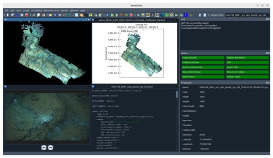
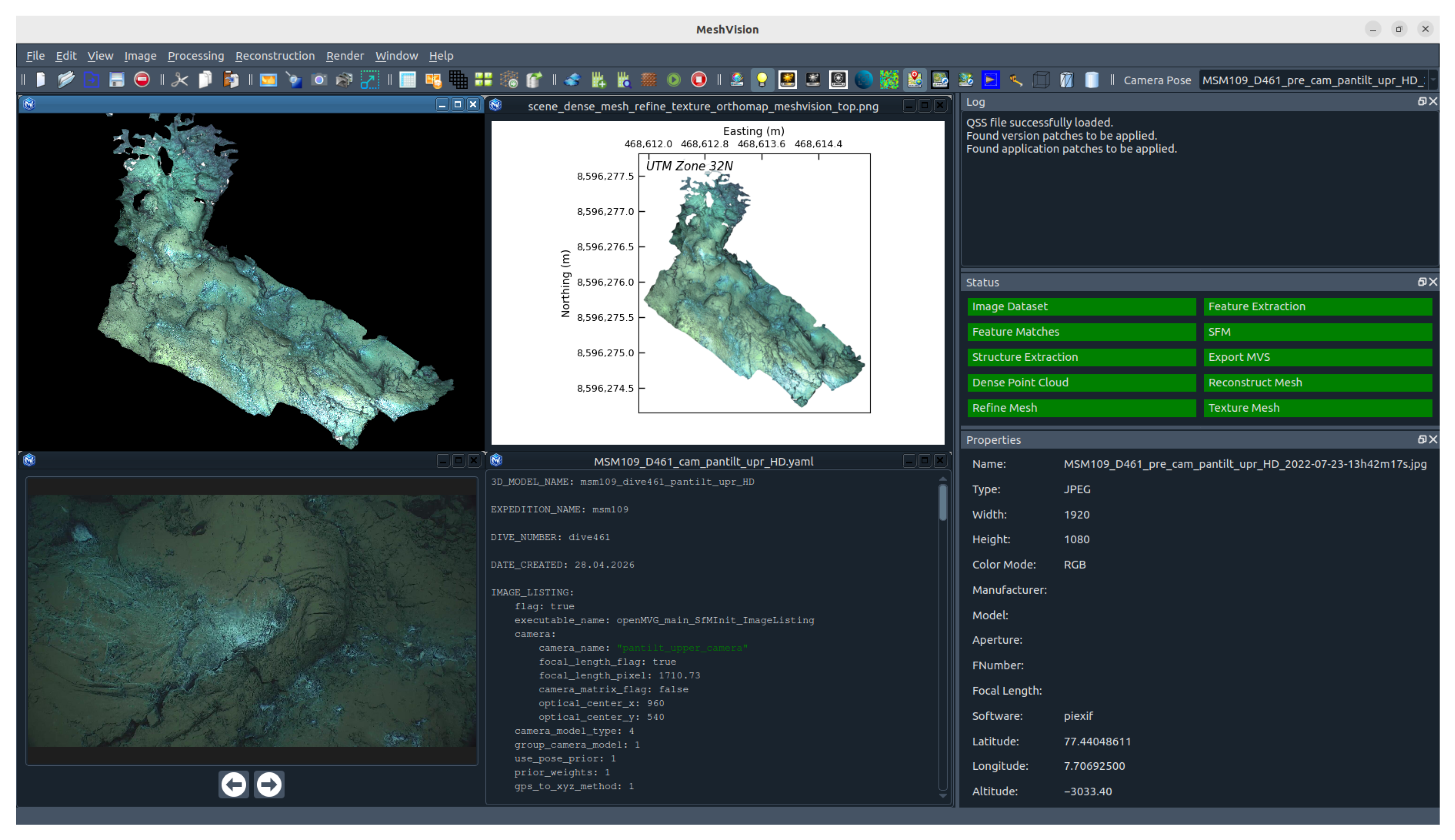
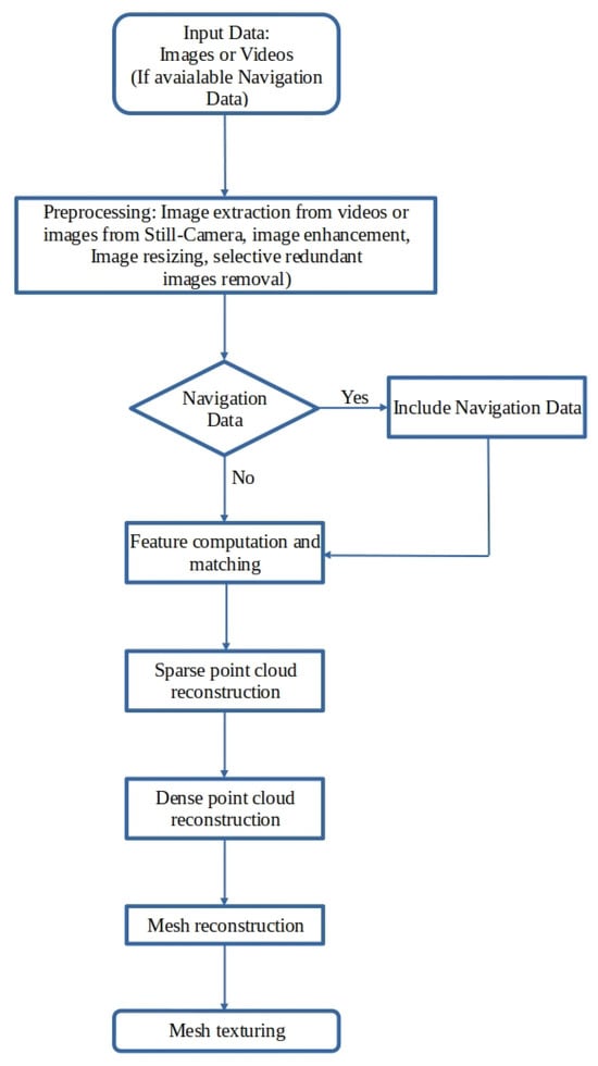
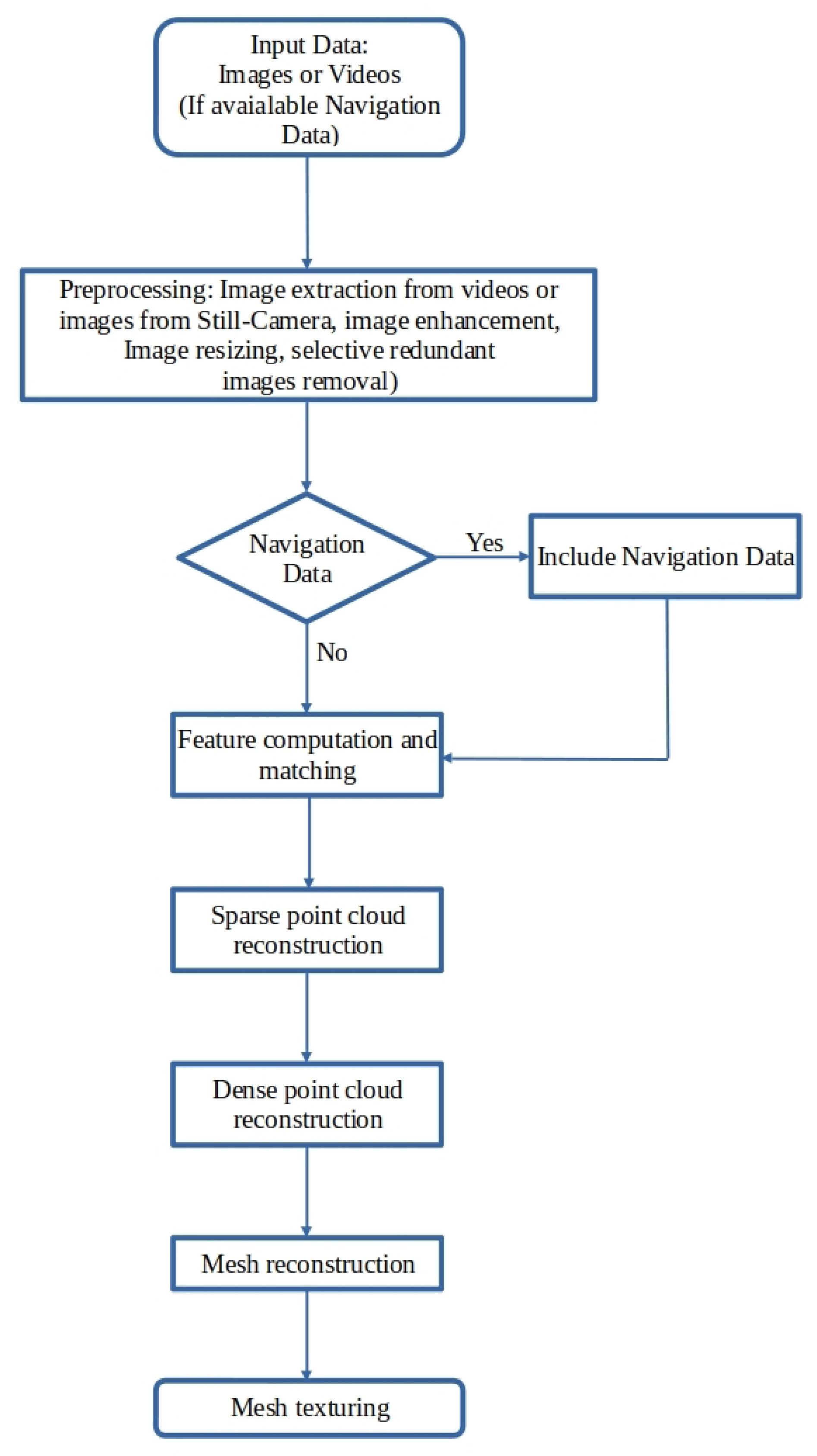
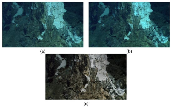
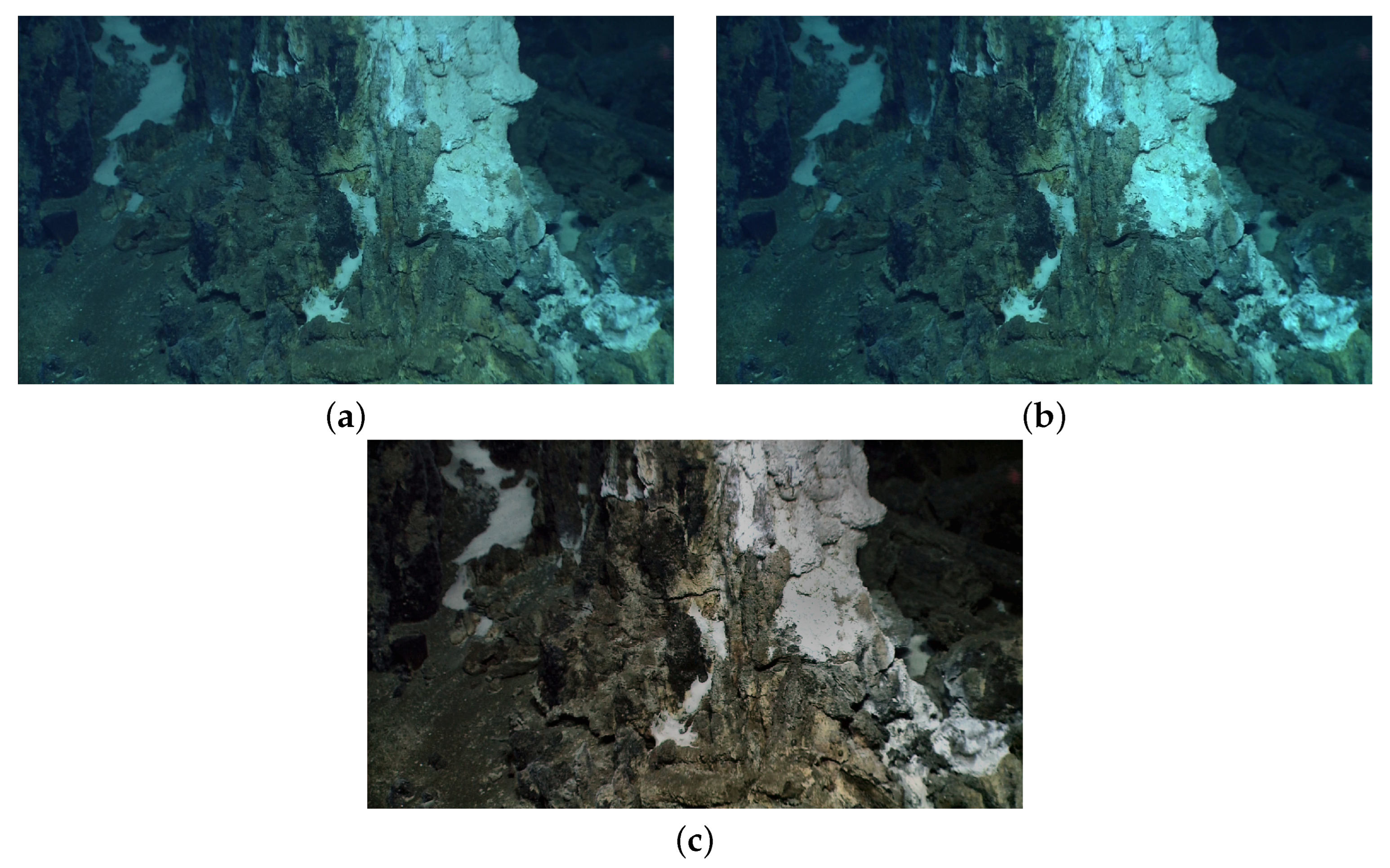
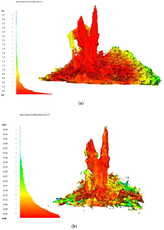
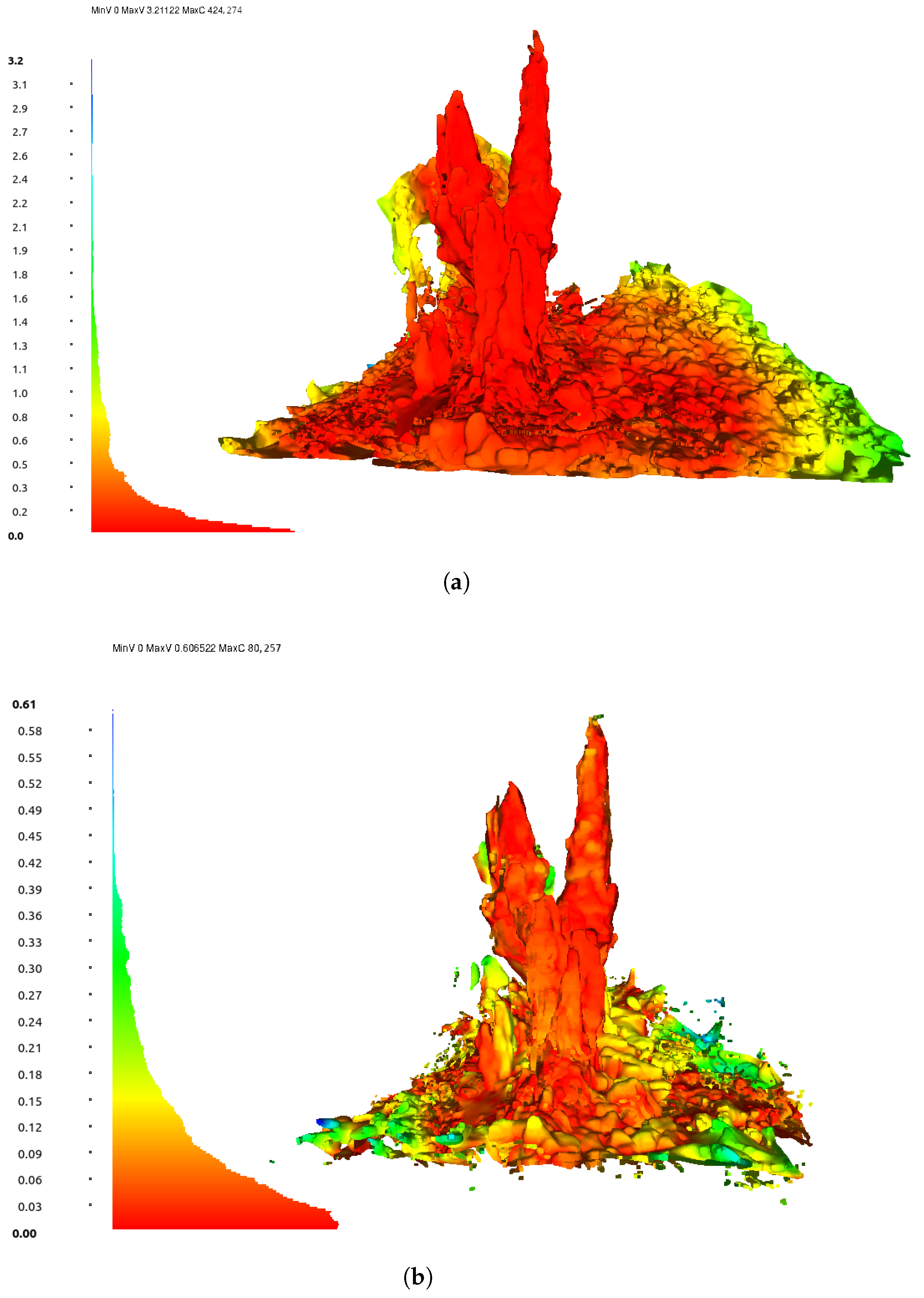
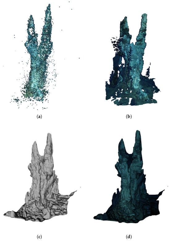
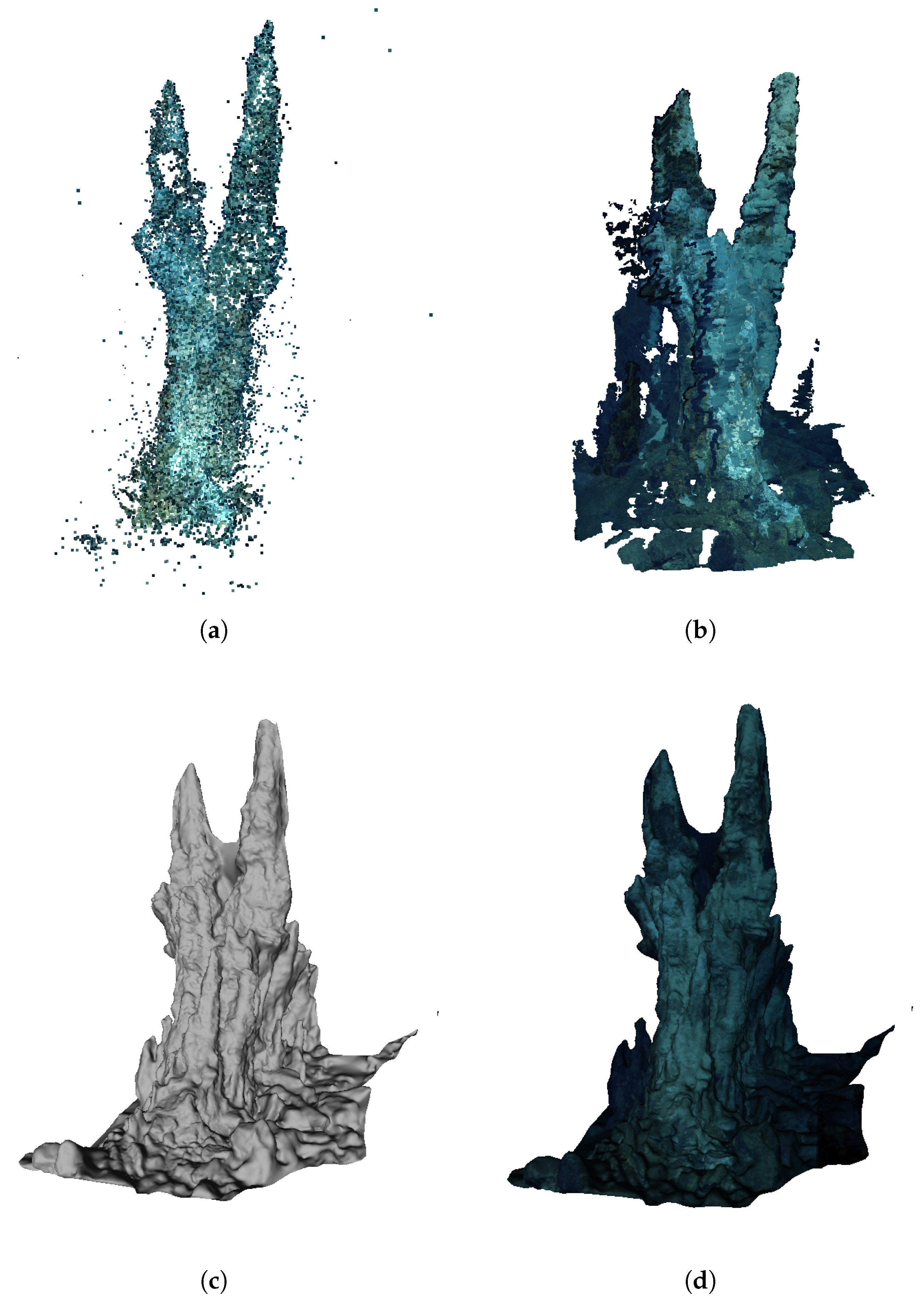
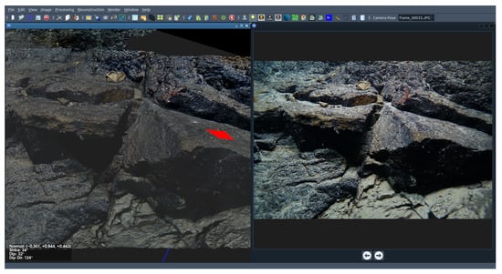
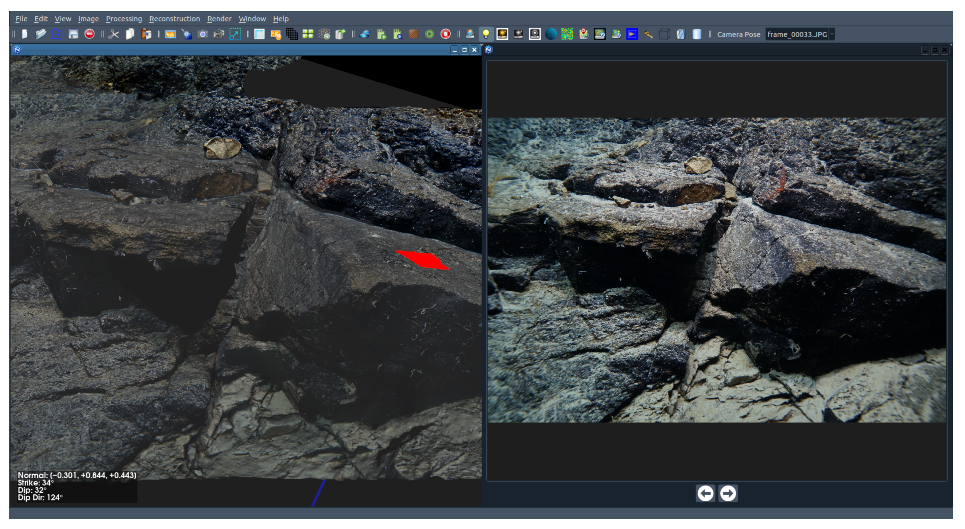
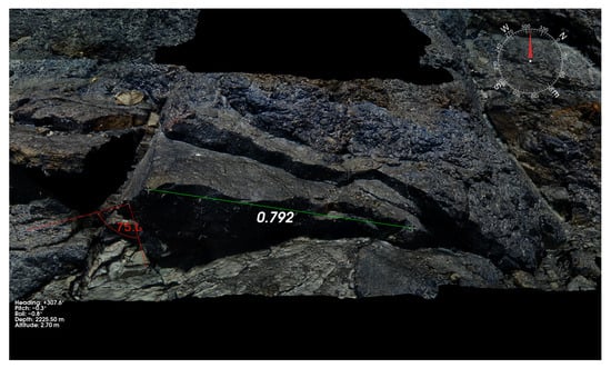
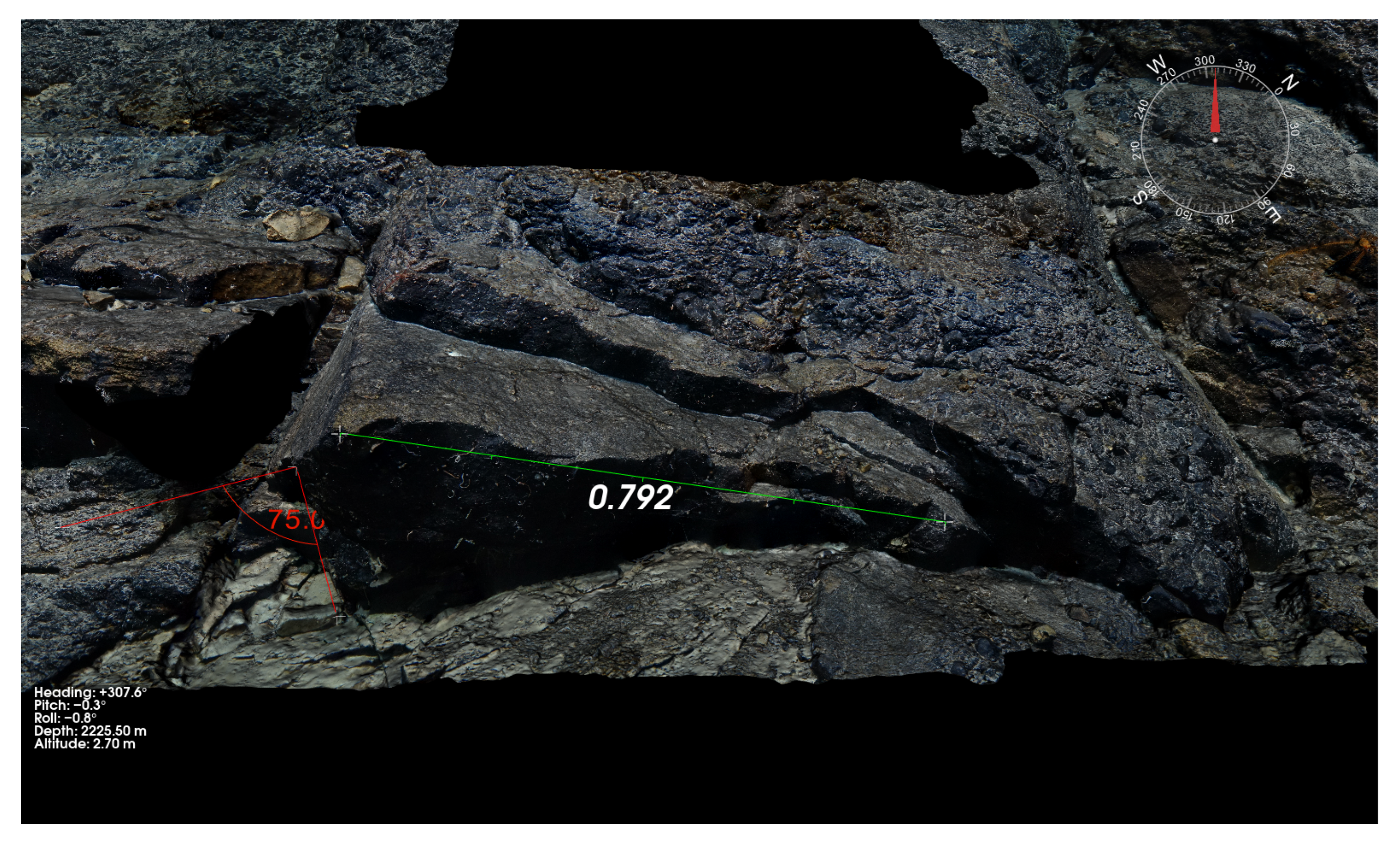
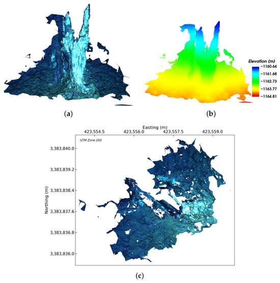
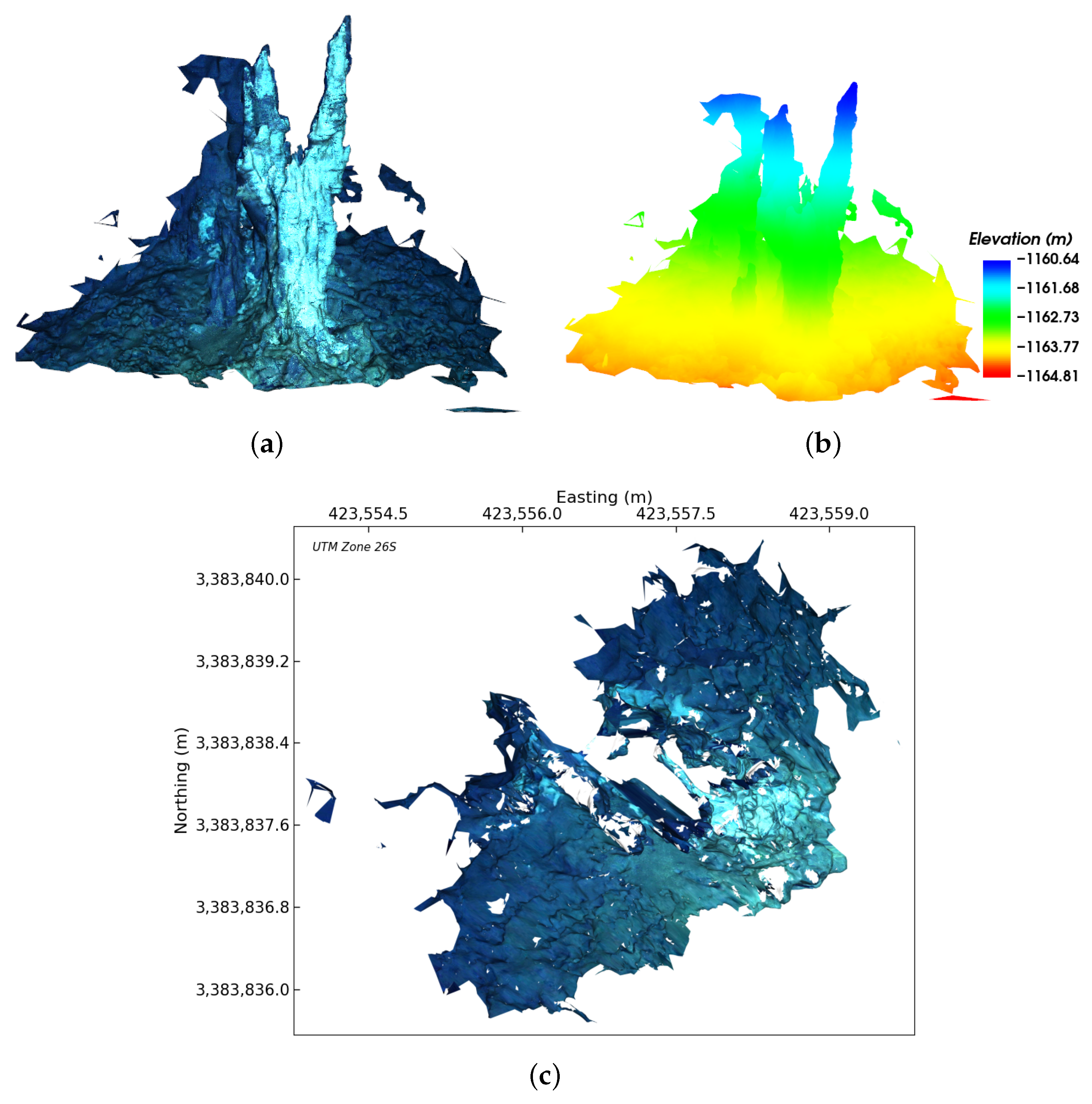
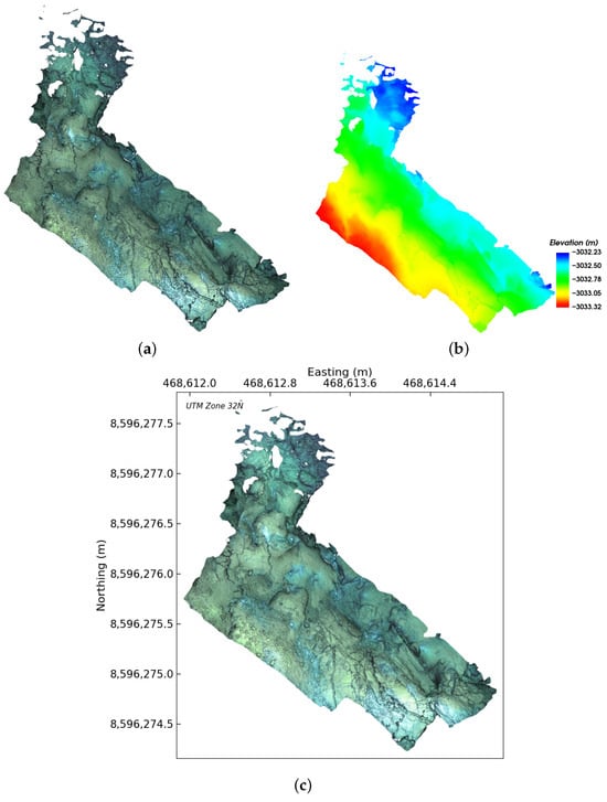
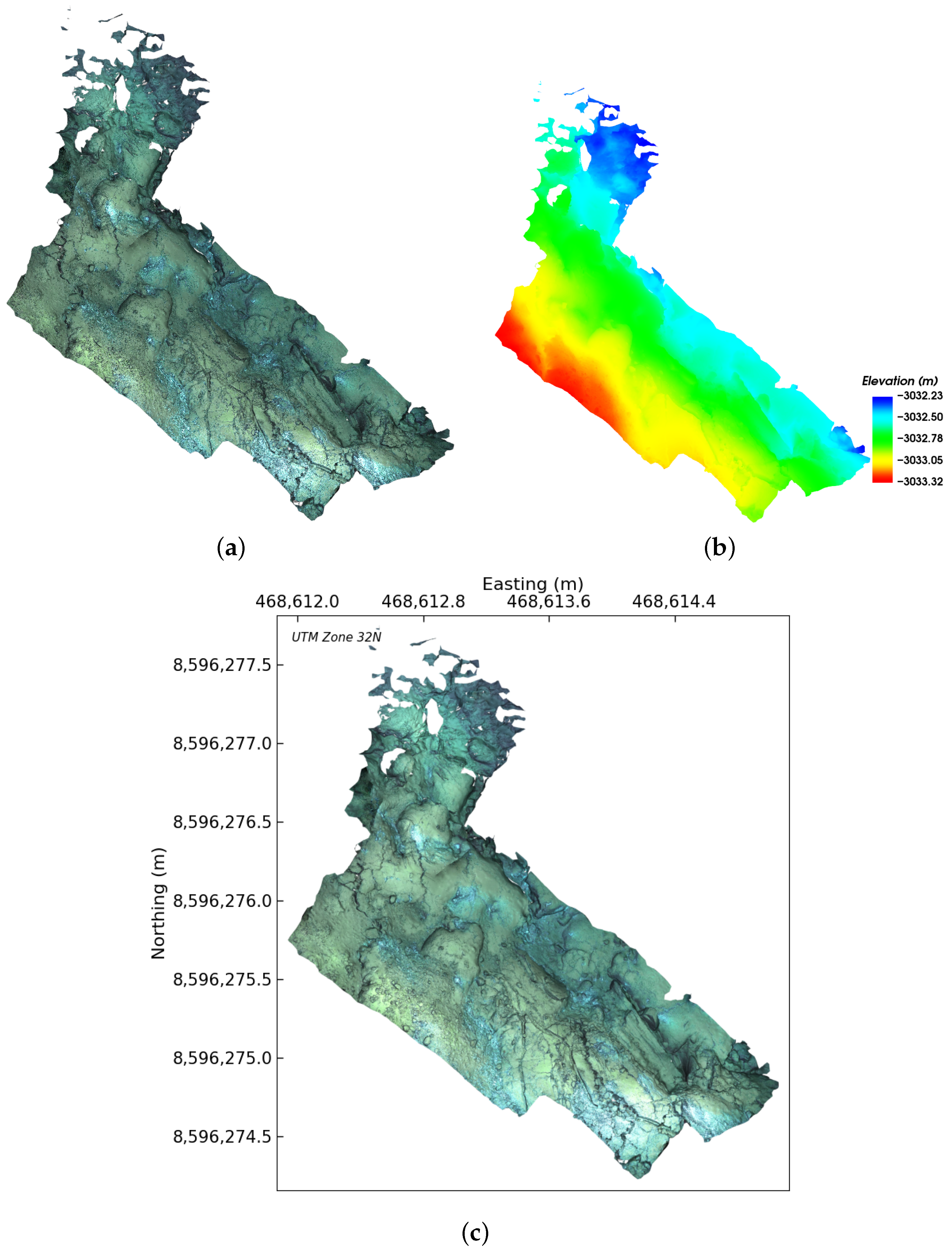
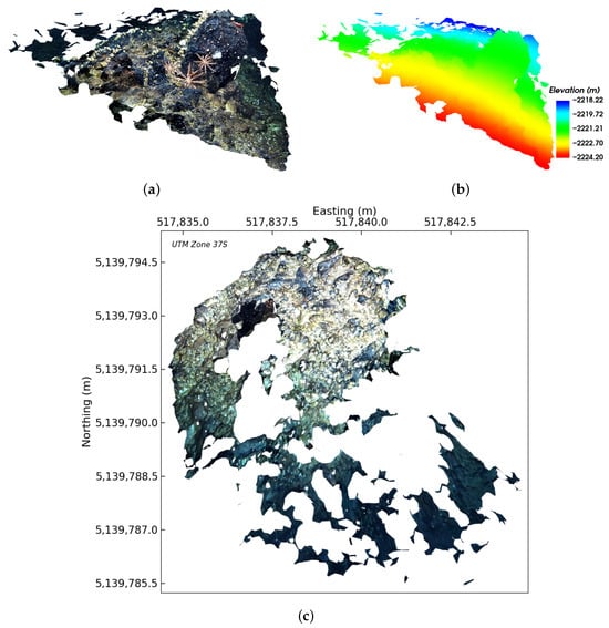
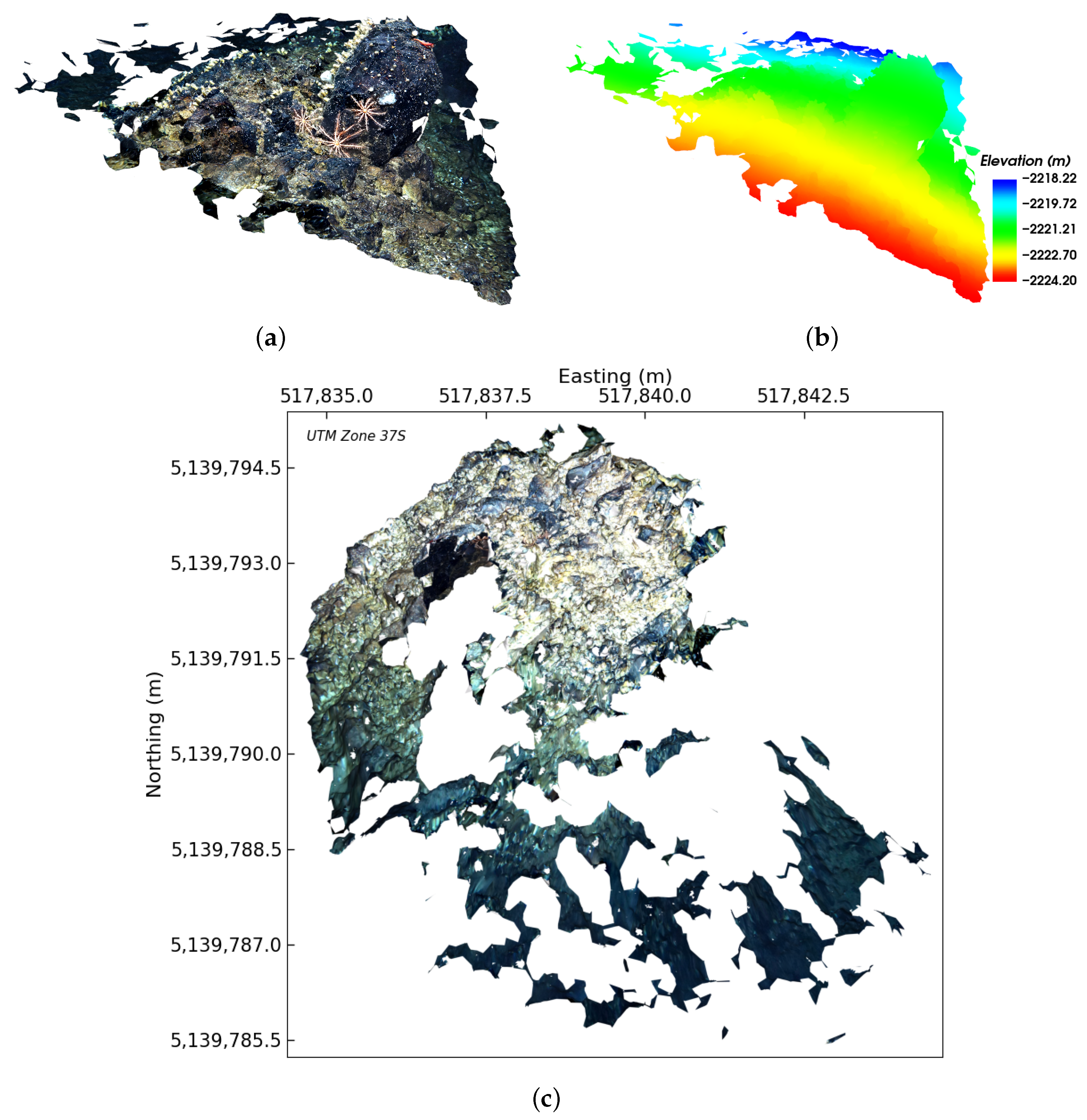
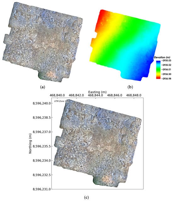
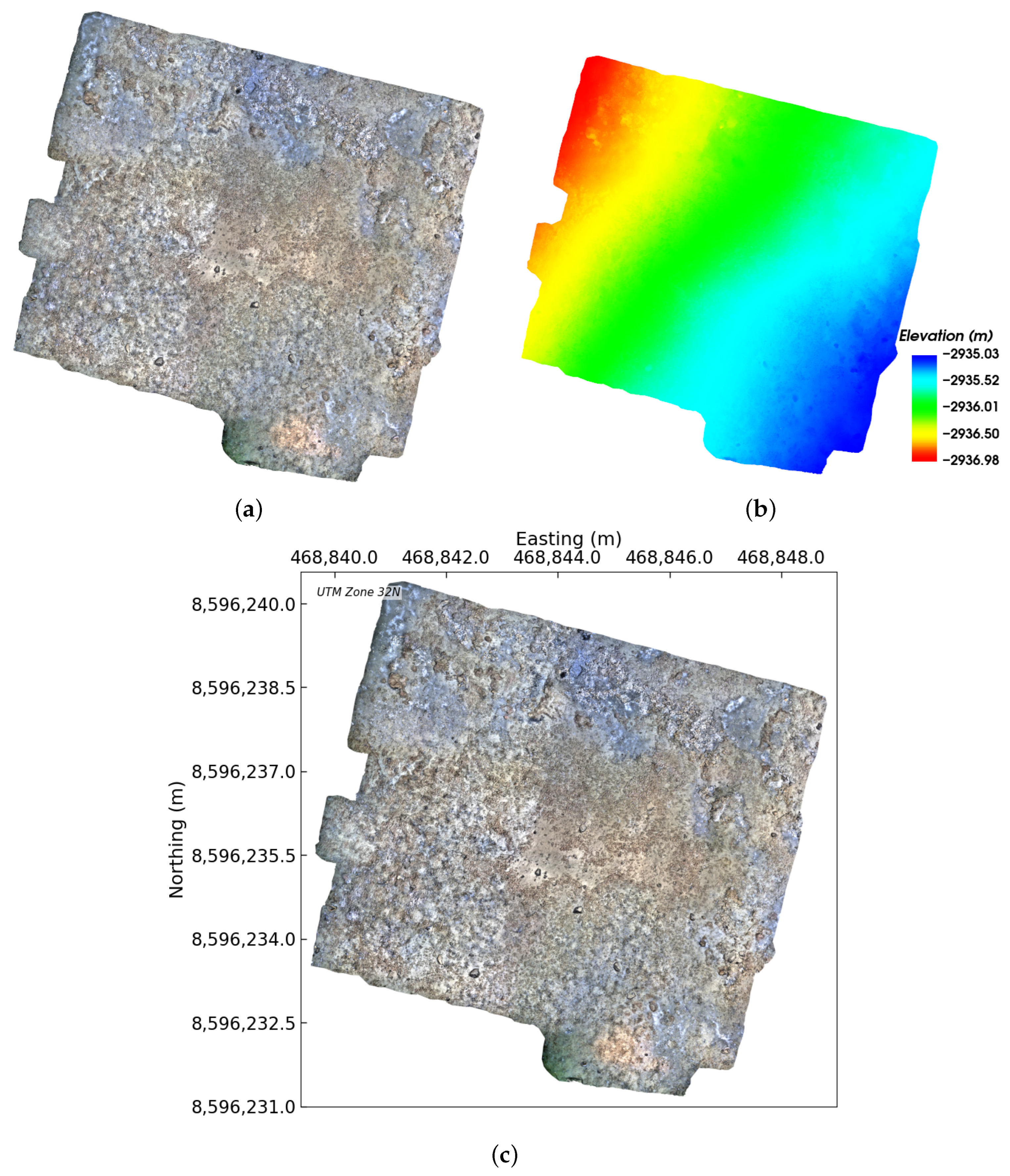

Disclaimer/Publisher’s Note: The statements, opinions and data contained in all publications are solely those of the individual author(s) and contributor(s) and not of MDPI and/or the editor(s). MDPI and/or the editor(s) disclaim responsibility for any injury to people or property resulting from any ideas, methods, instructions or products referred to in the content. |
© 2026 by the authors. Licensee MDPI, Basel, Switzerland. This article is an open access article distributed under the terms and conditions of the Creative Commons Attribution (CC BY) license.