


Abstract
Reliable weak target detection in nonstationary sea clutter is essential for maritime surveillance and navigation safety. Fluctuating sea-surface returns and evolving Doppler spectra can mask weak targets, while conditioning solely on the cell under test may introduce target components into the background representation. This paper proposes a reference-cell Doppler-conditioned Mamba autoencoder (RDC-Mamba) for unsupervised weak target detection. Time–frequency features from reference cells outside the guard regions are aggregated through masked attention and adaptive bilateral fusion to form a local Doppler prior. This prior modulates the state-update step size, input mapping, and output gate, linking temporal modeling to the surrounding clutter background. The network is trained on target-free clutter samples, and detection combines temporal complex-valued and multi-resolution spectral reconstruction errors. At a false-alarm probability of , RDC-Mamba outperforms classical CFAR detectors and the evaluated reconstruction-based baselines, achieving detection probabilities of 84.6% and 88.2% on IPIX and SDRDSP, respectively. Compared with Self-Doppler Mamba, the strongest competing baseline, the detection probabilities increase by 7.0 and 5.2 percentage points, respectively.
1. Introduction
Detecting weak maritime targets is a central task in maritime surveillance, navigation safety, and ocean monitoring. Small nonmetallic boats and low-profile floating objects can be difficult to detect when their weak or fluctuating echoes overlap the sea-clutter spectrum [1]. At low grazing angles, high-resolution radar returns from the sea surface exhibit non-Gaussian distributions, nonstationarity, strong temporal correlation, and heavy tails. Breaking waves and whitecaps can also generate sea spikes with large amplitudes, masking echoes from small floating targets [2]. Classical constant false alarm rate (CFAR) detectors estimate the background power using reference range cells surrounding the cell under test (CUT) and set an adaptive decision threshold. Clutter edges, multiple targets, and anomalous sea spikes within the reference window can bias this estimate and limit detection at low false-alarm probabilities [3].
Feature-based detectors characterize the differences between target returns and sea clutter in temporal, spectral, and multi-dimensional feature spaces. Shui et al. [4] combined relative amplitude, relative Doppler peak height, and the relative entropy of the Doppler amplitude spectrum into a three-dimensional representation for one-class detection of small floating targets. More recently, Guan et al. [5] used nonlinear dimensionality reduction to re-express echo features and based detection on feature-sample distances between the CUT and an adjacent reference cell. Guo et al. [6] described normal clutter using a dominant clutter tree within an anomaly-detection framework. These approaches connect feature-space structure with the surrounding background, but their performance remains sensitive to feature selection and changes in clutter distributions across sea conditions.
Recent deep-learning studies have explored multimodal fusion, lightweight representation learning, and probabilistic modeling. Wang and Wang [7] combined time–frequency images, phase sequences, and correlation-coefficient sequences in a triple-channel network, with detections produced by a false-alarm control unit. Yuan et al. [8] used adaptive multiscale convolution, hybrid pooling, and lightweight residual structures to balance maritime target feature extraction against computational cost. Wang et al. [9] introduced a two-stage framework that generates candidate regions and then classifies them to improve decision reliability. Bai et al. [10] developed a detection-oriented complex-valued variational autoencoder that jointly models amplitude and phase. These studies highlight the value of coordinating multidomain information with detection decisions. For long sea-clutter sequences, however, the coupling between local background conditions and temporal dynamics requires further investigation.
State-space models offer an efficient approach to long-sequence representation. Structured state-space models capture long-range dependencies at relatively low computational cost [11]. Mamba introduces input-dependent selection, allowing its update parameters to vary with the current input while retaining linear complexity in sequence length [12]. Recent applications combine CNNs and Mamba for maritime detection [13], while radar-modulated selection demonstrates how auxiliary measurements can condition selective scans [14]. Quasi-periodic motion, Doppler spreading, and time-varying correlation in sea clutter motivate the use of such dynamic models. When the CUT alone determines the selective updates, however, the network may have difficulty separating target-induced anomalies from changes in local sea conditions. Doppler conditioning derived directly from the CUT can also include target components, allowing them to enter the learned normal-background representation.
Reference cells provide a natural source of local background information. CFAR uses them to estimate background intensity, while the feature-distance method of Guan et al. [5] explicitly compares the CUT with an adjacent reference cell. Zhu et al. [15] investigated maritime target detection through multi-dimensional attention and autocorrelation modeling. These methods emphasize background relationships and feature dependencies, but the integration of reference-cell Doppler structure into the internal updates of a selective state-space model remains a specific design question. Conditioning layers can alter intermediate feature transmission using auxiliary information [16], providing a basis for incorporating local clutter priors into Mamba state updates.
This paper proposes RDC-Mamba, a reference-cell Doppler-conditioned autoencoder for weak target detection in sea clutter. Its contributions are threefold. First, it establishes a reference-conditioned clutter-modeling framework that describes normal CUT dynamics using Doppler information from the surrounding range cells. Second, it introduces a Doppler-conditioned selective state-update mechanism in which the reference prior modulates information writing, memory time scales, and output gating. Third, it evaluates the framework on IPIX and SDRDSP through low-false-alarm detection performance, component comparisons, record-level differences, cross-scenario limitations, and computational cost.
The remainder of the paper is organized as follows. Section 2 formulates the radar signal model and the reference-conditioned detection problem. Section 3 describes Doppler-prior extraction, conditional state updates, and the joint reconstruction-based detector. Section 4 presents the datasets, evaluation settings, detection results, component comparisons, cross-scenario analysis, and computational cost. Section 5 concludes the paper and discusses future work.
2. Radar Signal Model and Detection Problem
2.1. Radar Echo and Detection Model
Consider a complex-valued radar echo matrix acquired in staring mode over range cells and consecutive pulses:
Here, denotes the complete slow-time echo from range cell n. The model input comprises synchronized CUT and reference-cell windows extracted from the same record and slow-time starting point. Each window contains L pulses, with in general. In the following encoding, normalization, reconstruction, and detection operations, denotes the corresponding length-L window, and indexes its pulses. Thus, is the total number of pulses in the original record, whereas L consistently denotes the input window length. For the CUT at range cell , let . The detection hypotheses are
where , , and denote sea clutter, receiver noise, and the target echo, respectively. For a point target with approximately uniform motion over the observation interval, the slow-time echo can be expressed as
where is the normalized target Doppler frequency, measured in cycles per pulse with physical frequency , and and represent amplitude fluctuations and additional phase variations caused by target fluctuations, wave modulation, and micromotion. Floating targets generally depart from a strictly single-frequency model; this expression describes how their time–frequency structure can differ from the local clutter background.
Sea-clutter fluctuations are commonly described by compound-Gaussian texture–speckle models and K-distributed amplitudes [2]. Their non-Gaussian and time-varying characteristics motivate learning the normal CUT response from its local reference background.
2.2. CUT, Guard Cells, and Reference Cells
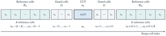
G guard cells and K reference cells are placed on each side of the CUT. The left and right reference sets are
The guard cells reduce contamination of the reference region by target range extent, while the reference cells describe the surrounding clutter. The reference-conditioned formulation relies on local background correlation: echoes within a limited range neighborhood are affected by similar sea conditions and radar operating states and therefore share correlated dominant Doppler structure. Local amplitude and spectral shape may vary gradually with range. This condition does not require the CUT and reference cells to be independent and identically distributed.
A reference encoder maps the two sets to a conditioning vector:
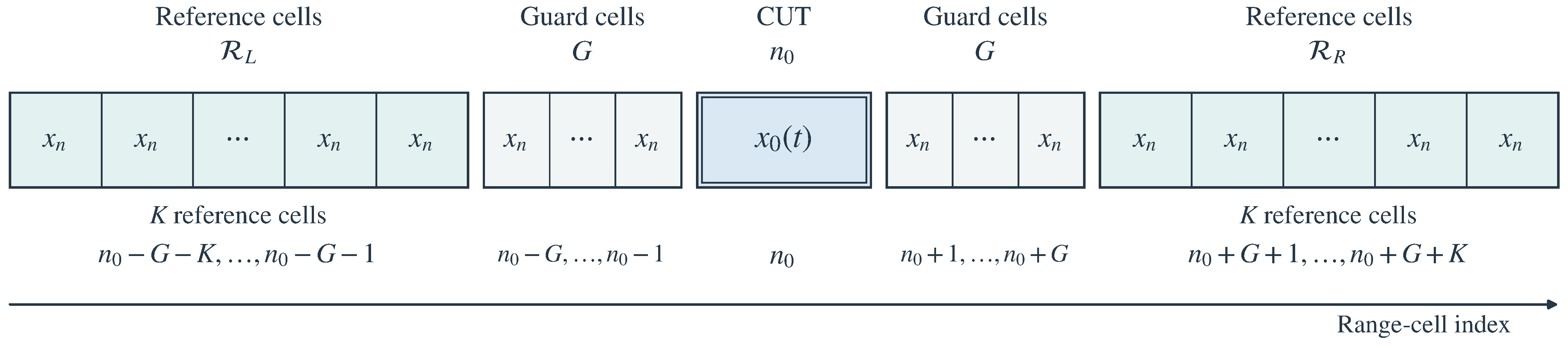
This vector describes the neighboring Doppler background and conditions the subsequent model. Figure 1 shows the range-window configuration, with guard regions separating the central CUT from the bilateral reference regions. The guard regions limit target leakage, and the reference regions provide local background information. The values of G and K follow the dataset settings in Section 4.1; guard cells are excluded from the reference encoder.
Figure 1.
CUT, guard cells, and bilateral reference cells.
2.3. Reference-Conditioned Anomaly Detection
A conventional unsupervised reconstruction model approximates the global normal distribution . To account for variations in clutter distributions across sea conditions, range, and observation time, this paper models the normal CUT distribution conditionally on the reference information:
Let denote the conditional autoencoder. Its reconstructed CUT is
The network is trained using target-free clutter samples to reconstruct normal CUT dynamics under the reference-background condition. Target-induced deviations in the temporal or spectral structure are characterized by reconstruction discrepancies. This paper defines the reconstruction-based detection statistic as
and makes the decision using
where is calibrated from clutter-only validation samples for a prescribed false-alarm probability.
3. Reference-Cell Doppler-Conditioned Mamba Detector
3.1. Overall Architecture
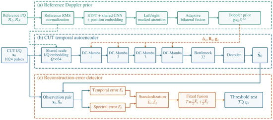
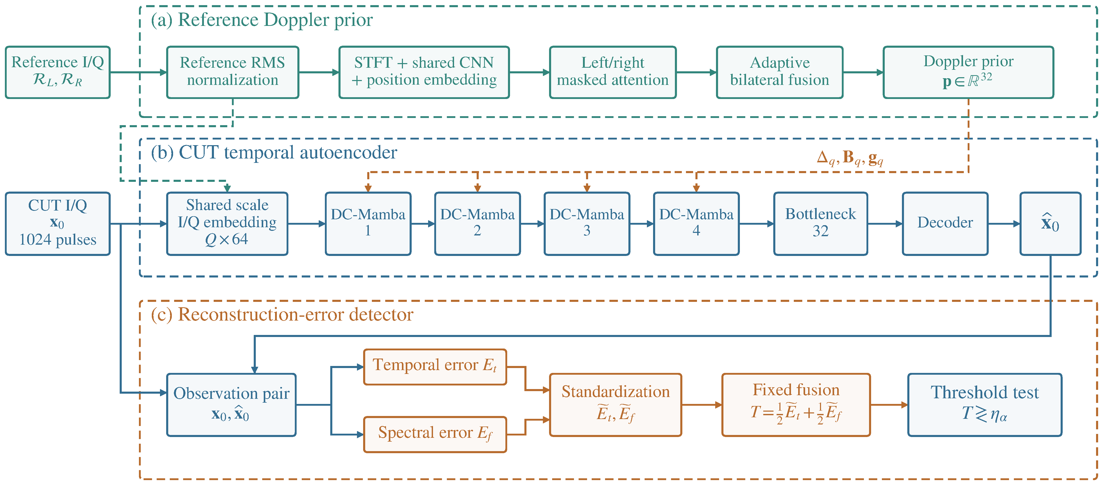
As shown in Figure 2, RDC-Mamba comprises a reference Doppler-prior branch, a temporal CUT encoder, four Doppler-conditioned Mamba (DC-Mamba) blocks sharing the reference prior, and a lightweight decoder. The DC-Mamba blocks perform selective state updates under the reference-background condition. The reference branch processes the surrounding background echoes, while the CUT branch receives the complex-valued slow-time sequence. The two branches interact through modulation inside the DC-Mamba blocks, producing a temporal reconstruction network conditioned on the local background.
Figure 2.
Overall architecture and detection pipeline of RDC-Mamba. Teal, blue, and orange panel borders distinguish the reference-prior, CUT-reconstruction, and detection branches, respectively. Solid arrows show signal flow; the teal dashed path supplies the shared normalization scale, and orange dashed arrows carry the reference prior.
The reference branch applies the short-time Fourier transform (STFT) to represent local spectral shape and its evolution, while the CUT branch directly encodes the complex-valued temporal sequence. Once the background prior is obtained, each DC-Mamba block uses it to modulate the state-update parameters. The encoded features pass through the bottleneck and decoder to reconstruct the CUT echo, and a joint reconstruction-error statistic produces the detection decision. The CUT itself is excluded from the reference branch to reduce the risk of target spectral information entering the background condition.
3.2. Reference-Cell Doppler-Prior Extraction
Following bilateral reference-cell selection, the synchronized echo windows are normalized to reduce the effects of propagation loss and gain differences on the background representation. A median root-mean-square scale is estimated from the valid reference echoes of length L:
where . The CUT and reference echoes share the scale , where prevents division by zero and logarithms of zero. Computing the scale from reference cells alone excludes target amplitude in the CUT from background normalization. This design draws on the treatment of distribution changes through sequence normalization in RevIN [17], but estimates a common scale from the reference cells to preserve relative CUT-to-background amplitude.
After normalization, an STFT maps the echo from reference cell r to a local time–frequency representation:
where is the analysis window, and , H, and are the window length, hop size, and FFT size, respectively [18]. The spectral encoder receives the log-power feature
A shared lightweight convolutional encoder maps to a reference feature , with an embedding of the actual relative range position. The left and right reference sets are then aggregated separately using masked attention to accommodate variation in the number of available cells. For ,
where indicates whether a reference cell is valid. The aggregation combines permutation-invariant set processing with learnable attention weights [19,20].
The left and right representations, and , and their difference determine the bilateral fusion weights:
The fused prior is
Figure 3 summarizes the sequence of reference normalization, STFT, shared spectral encoding, side-specific aggregation, and adaptive fusion. During training, reference cells are randomly masked with probability to reduce reliance on individual range positions. The resulting prior conditions the state updates in the CUT branch.
Figure 3.
Reference-cell Doppler-prior extraction.
3.3. Doppler-Conditioned Selective State Updates
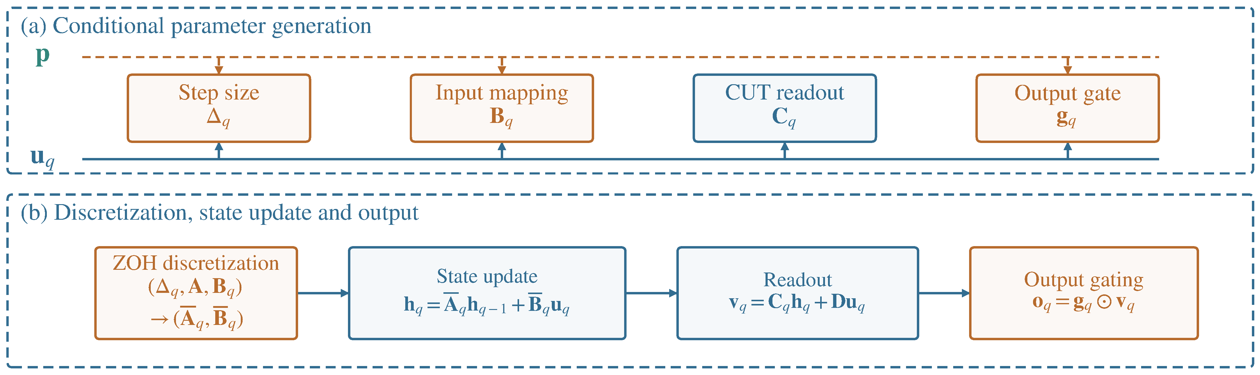
Once the reference prior is available, the CUT branch represents the real and imaginary parts of the complex sequence as two real-valued channels. A one-dimensional convolutional embedding produces Q temporal feature vectors . To incorporate the background condition into the temporal dynamics, the continuous-time state-space representation serves as the starting point:
where is the hidden state, is the state matrix, and and are the input and output mappings. Mamba generates input-dependent discretization parameters, enabling selective writing or suppression of current information [12].
The conditional update parameters are generated from both the local CUT feature and the reference prior :
The step-size vector controls the memory time scale, determines how current information enters the state, and controls the feature output. The readout depends only on the CUT feature so that the reference prior does not directly determine the reconstructed content. To obtain decaying homogeneous state dynamics, a real diagonal state matrix parameterized by is adopted:
Here, is the state dimension. The exponential is applied separately to each real-valued diagonal parameter, giving and for . The shared matrix is learned rather than generated dynamically from the reference prior. The updates below are evaluated separately for each feature channel; denotes the corresponding component of , with the channel index omitted.
The matrix is the continuous-time input mapping. With zero-order-hold discretization, and denote the discrete state-transition matrix and input mapping, respectively:
The exponential is a matrix exponential. Because is diagonal, it reduces to exponentiation of the diagonal entries, which lie in after discretization. This establishes decay of the unforced state components; it does not establish stability of the complete network with conditional inputs.
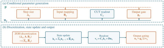
As shown in Figure 4, the reference prior affects state memory, information writing, and output control through , , and , respectively.
Figure 4.
Doppler-conditioned state update and readout. Blue arrows show signal flow, and orange dashed arrows show reference-prior modulation of the step size, input mapping, and output gate. Symbols are defined in the text.
DC-Mamba blocks are stacked using residual connections, normalization, and feedforward mappings to progressively represent CUT dynamics under the same local background condition. Conditioning the internal updates is intended to reduce reconstruction discrepancies associated with normal background changes while retaining anomalous CUT responses.
3.4. Decoder and Training Objective
After conditional state updating, the encoder output passes through a low-dimensional bottleneck to a decoder consisting of one-dimensional convolutions and upsampling layers. The decoder reconstructs the real and imaginary parts of the CUT. To encourage background-conditioned reconstruction, the original CUT is not directly connected to the output through a skip connection, and the reference prior is not supplied directly to the decoder.
For the reconstructed echo , the temporal loss over the length-L CUT window is
To capture differences in local spectral peaks, bandwidth, and shape, the training objective additionally incorporates a multi-resolution STFT loss with M analysis configurations [21]:
The training objective uses the calligraphic symbol , distinguishing it from the window length L:
Joint representation of the real and imaginary components preserves coupled amplitude and phase information [22]. Its contribution relative to amplitude-only input can be examined through an input-representation comparison.
3.5. Detection Statistic
At detection time, discrepancies between the CUT input and its reconstruction quantify departures from the learned background. To reduce the influence of record-dependent amplitude scales, the temporal error is normalized as
The spectral error is the multi-resolution spectral discrepancy used in the training objective. After separate standardization, the temporal and spectral errors are combined as
where and are the standardized temporal and spectral errors. The standardization is
The parameters and are estimated from the corresponding errors of clutter-only training windows within the current fold and are frozen for validation and testing. The fusion weights satisfy and and are distinct from the training-loss weights and . Fixed equal weighting, , is applied after separate error standardization. These weights are neither converted from the loss weights nor tuned on validation or test data. Clutter-only validation loss is used for checkpoint selection and early stopping. After the checkpoint is fixed, clutter-only validation scores calibrate the threshold; they are not used to tune the error-fusion weights. For a prescribed false-alarm probability , the threshold is the empirical quantile of clutter-only validation statistics:
Threshold calibration is part of the detection-evaluation procedure and is separate from network-parameter learning.
3.6. Computational Complexity
The additional computational cost of the reference branch is evaluated alongside detection performance. With K reference cells per side, Q STFT frames, and FFT size , its principal cost is approximately
The DC-Mamba scan has linear complexity in sequence length Q, approximately , where d and are the feature and state dimensions. This scaling is advantageous for long pulse sequences compared with the quadratic sequence complexity of global self-attention.
4. Evaluation Settings and Results
4.1. Datasets and Observation Scenarios
This paper evaluates the proposed method using the publicly available McMaster University IPIX radar data [23,24] and the Yantai data released by the Sea-Detecting Radar Data Sharing Program (SDRDSP) [25,26,27]. Differences in range coverage, target characteristics, and observation configurations provide distinct clutter backgrounds for evaluation.
The IPIX data were acquired in 1993 near Dartmouth, Canada, using a fully coherent X-band radar with a center frequency of approximately 9.39 GHz, pulse repetition frequency (PRF) of 1 kHz, and range resolution of approximately 30 m. Each staring record contains 131,072 pulses and 14 range cells, with HH, VV, HV, and VH polarization channels. The observed target was a floating sphere approximately 1 m in diameter covered with metallic material. Records 280, 311, and 320 are selected for analysis. Table 1 lists their primary target cells and environmental conditions. The primary target cell defines target samples; neighboring affected cells are excluded from training and threshold estimation.
Table 1.
IPIX records, target cells, and environmental conditions. # denotes the record number.
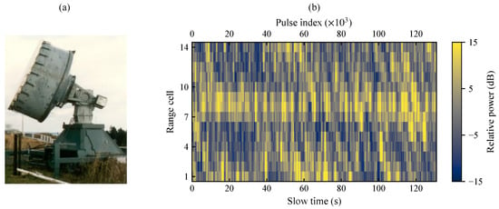
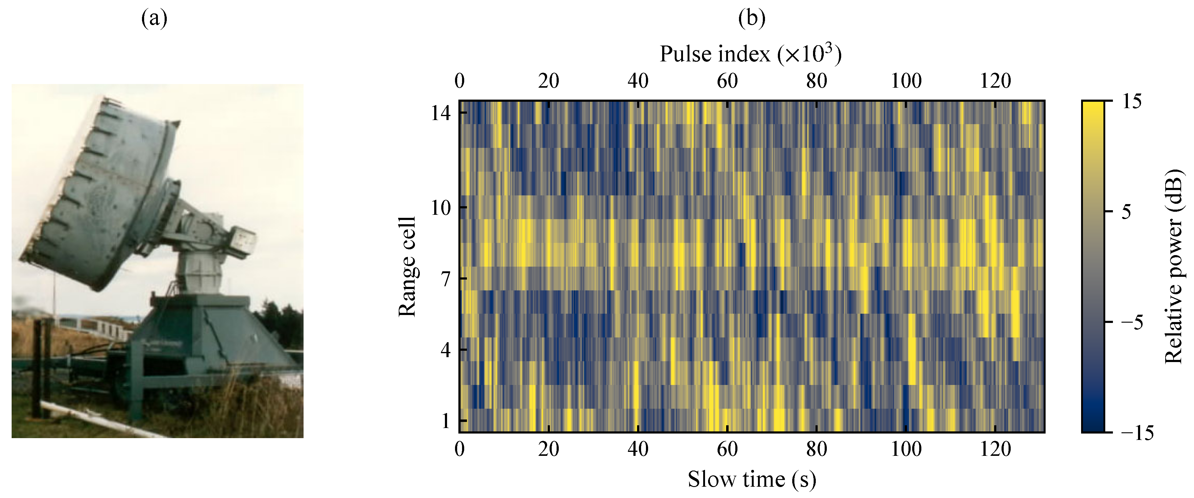
Figure 5 shows the radar platform and the slow-time–range distribution of the HH-polarized echo in record #280. The echo panel covers all 14 range cells. Power is averaged over groups of 256 pulses and converted to relative decibels using the median power of the entire image as the reference, allowing the background fluctuations and their range distribution to be inspected.
Figure 5.
IPIX radar and echo distribution. (a) Radar platform [24]; (b) slow-time–range relative power for record #280.
The SDRDSP staring records used here were acquired on 4 and 6 January 2021 and are provided in the officially named “2020 Series, Issue 1” dataset, released in February 2021 [27]. Table 2 summarizes the record metadata. Performance analysis uses the beacon record 20210106150614_01_staring. The echo-distribution panel uses 20210104163843_01_staring from the same release to show its slow-time–range structure.
Table 2.
SDRDSP record metadata.
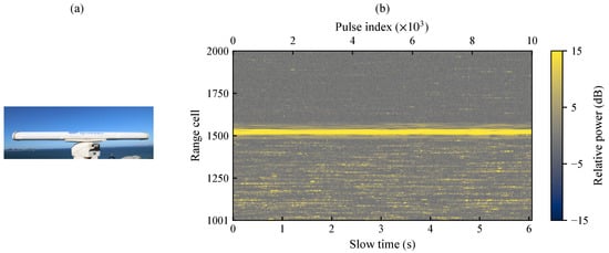
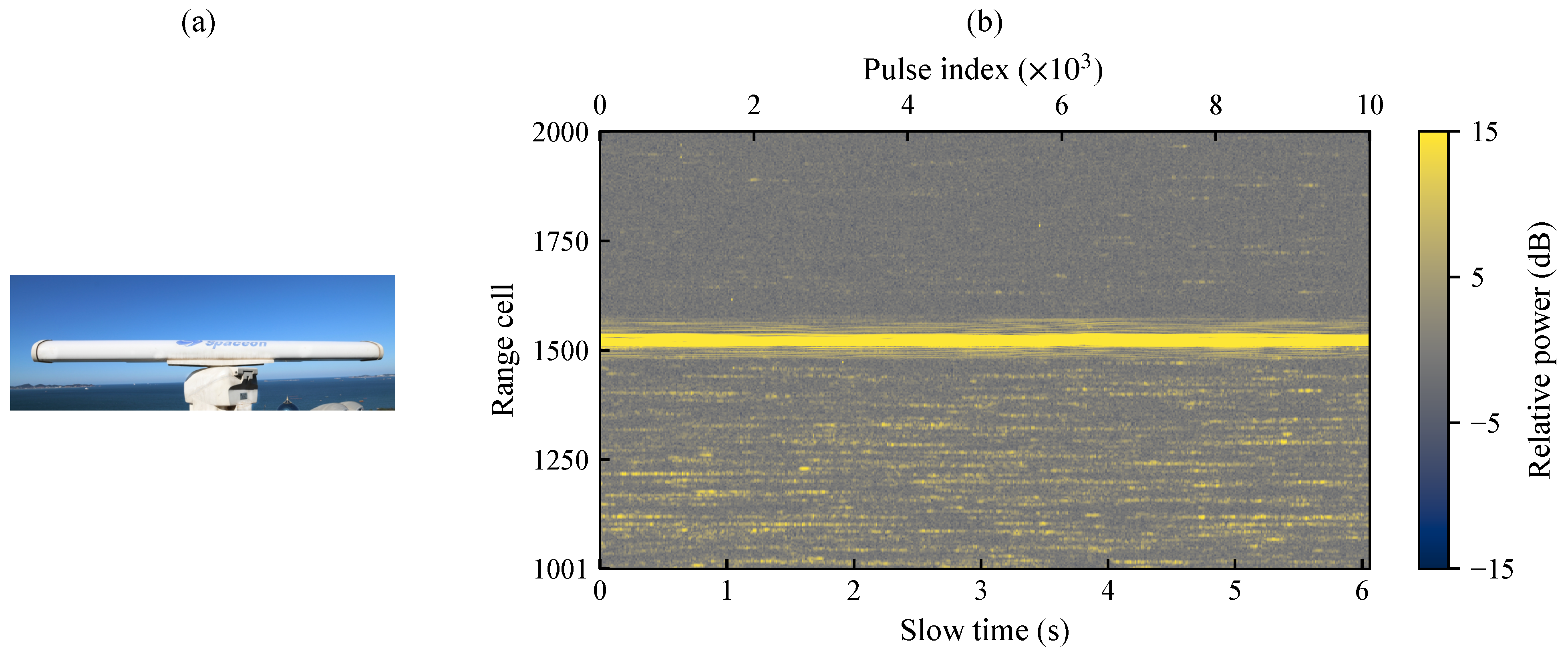
Figure 6 shows the SDRDSP radar and the broader range coverage of the recorded echoes. The echo panel uses the T1 complex-valued data and displays range cells 1001–2000, with power averaged over groups of 20 pulses. It uses the same relative-power definition and color scale as the IPIX panel. Slow time is obtained from the nominal record PRF.
Figure 6.
SDRDSP radar and echo distribution. (a) Radar platform [25]; (b) slow-time–range relative power.
For IPIX, the guard-cell and reference-cell counts are set to and , respectively, yielding at most six reference cells per CUT. Primary target cells, affected cells, and out-of-bounds positions are excluded by masks; missing reference cells are not duplicated or padded with copied data. Because SDRDSP targets can occupy multiple range cells, its reference configuration uses and . The limited IPIX range coverage constrains spatial background sampling, while each available cell still provides a slow-time sequence. The applicability of the local Doppler prior depends on CUT-to-reference background correlation and reference quality.
4.2. Sample Construction and Data Partitioning
Each sample contains synchronized CUT and reference pulses. Training uses stride 512; validation and testing use nonoverlapping windows with stride 1024. Original files remain disjoint within each split. The primary-target CUT provides H1; affected CUTs are excluded from H0 and H1 evaluation, and other valid CUTs provide H0. Only H0 CUTs are used for training, validation loss and threshold calibration.
IPIX uses three record-level folds: training/validation/testing records are 280/311/320, 311/320/280 and 320/280/311. Each fold contains 2550 training H0 windows, 1280 validation H0 windows and 1280 test H0 plus 128 test H1 windows. Each training CUT supplies 255 windows; evaluation covers 128 temporal windows. Validation H0 is reused for checkpoint selection and threshold calibration and is counted once. Normalization statistics are estimated from training H0, and weights, score standardization and thresholds are fixed for testing.
The reconstruction illustration and runtime evaluation use the configuration specified in Section 4.3. Its training records 17/26/40/54 contain 640/704/640/640 H0 windows, with record 30 providing 1408 validation H0 and record 280 providing 1280 calibration H0. Test records 19/25/283/310 contain 1408/1408/1152/1280 H0 and 128 H1 windows each. Training selects 64 nonoverlapping windows per CUT. References in this configuration follow guard and boundary rules without label-based cleaning, whereas the three-fold protocol masks known target and affected reference positions. All sample counts refer to range-cell–window pairs, not independent temporal observations.
4.3. Network Configuration and Training Protocol
The reference-branch STFT uses a Hann window of length 128, a hop size of 32, and an FFT size of 128. The CUT embedding dimension is , the reference-prior dimension is , and the state dimension is . The encoder contains four DC-Mamba blocks and a bottleneck of dimension 32. The multi-resolution spectral loss uses window lengths of 64, 128, and 256 with hop sizes of 16, 32, and 64, respectively. The training-loss weights are and . The detection-error fusion weights are fixed at in every fold without additional weight tuning.
The training configuration uses AdamW [28] with an initial learning rate of , weight decay of , batch size of 64, and a maximum of 200 epochs. Training stops when the validation loss does not improve for 20 consecutive epochs. The random seeds are 17, 23, and 29. The runtime environment and measurement protocol are specified in Section 4.8.
At inference, reference conditions are recomputed per synchronized window while learned weights remain fixed. Threshold recalibration and network retraining are different operations; a fixed deployment retraining interval is not established by these experiments.
For the reconstruction illustration and runtime benchmark, the evaluated implementations use the following settings: RDC-Mamba has patch stride eight, temporal/prior/state widths 32/16/8 and 17,333 parameters; CNN-AE uses convolution channels; LSTM-AE has a two-layer width-32 encoder, a width-16 bottleneck and a one-layer width-32 decoder. The VAE uses a 32-dimensional latent vector and KL weight 0.001, with posterior-mean inference. Unconditioned and self-conditioned SSMs retain the compact CUT backbone. These implementations use AdamW, learning rate , batch size 32 and 20 epochs, with minimum H0-validation loss selecting the checkpoint.
4.4. Comparison Methods and Evaluation Metrics
The comparison includes CA-CFAR and OS-CFAR [3], CNN-AE, LSTM-AE, VAE, a Mamba autoencoder (Mamba-AE), and Self-Doppler Mamba, which extracts its Doppler condition from the CUT itself. Mamba-AE and RDC-Mamba share the temporal backbone and decoder so that the comparison focuses on the reference prior and conditional state updates rather than differences in backbone architecture.
The detection and false-alarm probabilities are
This paper reports receiver operating characteristic (ROC) curves and the area under the ROC curve (AUC) to assess detection performance [29].
All trainable models use seeds 17, 23 and 29. Metrics are computed separately for each run and averaged equally; seed SD is the sample standard deviation. Fixed-data CA-CFAR and OS-CFAR are deterministic and have zero seed SD. AUC confidence intervals use 1000 circular time-block bootstrap replicates, with block length eight and sensitivity checks at four and sixteen windows [30]. Within each record, shared temporal indices are used across cells, seeds and methods. Each replicate averages seed-specific metrics; the 2.5th and 97.5th percentiles define the interval. These intervals describe sample uncertainty conditional on the fitted models and observed scenes.
4.5. Overall Detection Performance
ROC curves, AUC values, and detection probabilities at fixed false-alarm operating points are used together to assess overall discrimination and low-false-alarm performance.
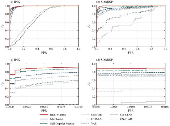
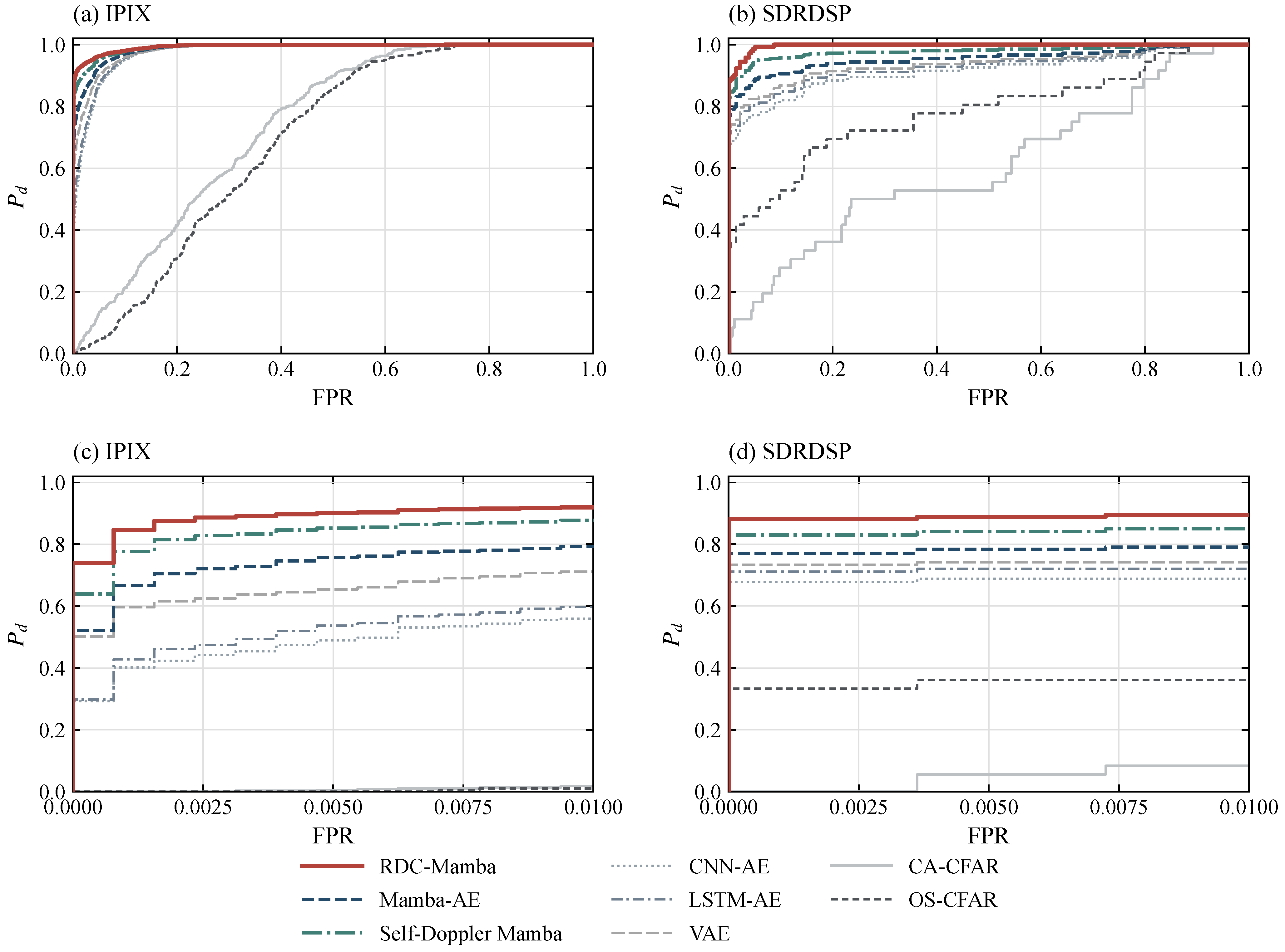
Figure 7 presents both the full ROC curves and the low-false-alarm region, with the principal metrics summarized in Table 3. At , RDC-Mamba achieves detection probabilities of 84.6% on IPIX and 88.2% on SDRDSP. These values exceed those of Mamba-AE by 18.0 and 11.2 percentage points and those of Self-Doppler Mamba by 7.0 and 5.2 percentage points, respectively. The ROC curves use a stepwise representation with equal weighting across records. AUC describes discrimination over the complete curve, while fixed-operating-point detection probability characterizes the low-false-alarm region.
Figure 7.
ROC curves for the comparison methods. (a,b) Full ROC curves; (c,d) low-false-alarm regions.
Table 3.
Detection performance of the comparison methods. values are probabilities.
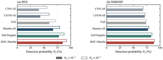
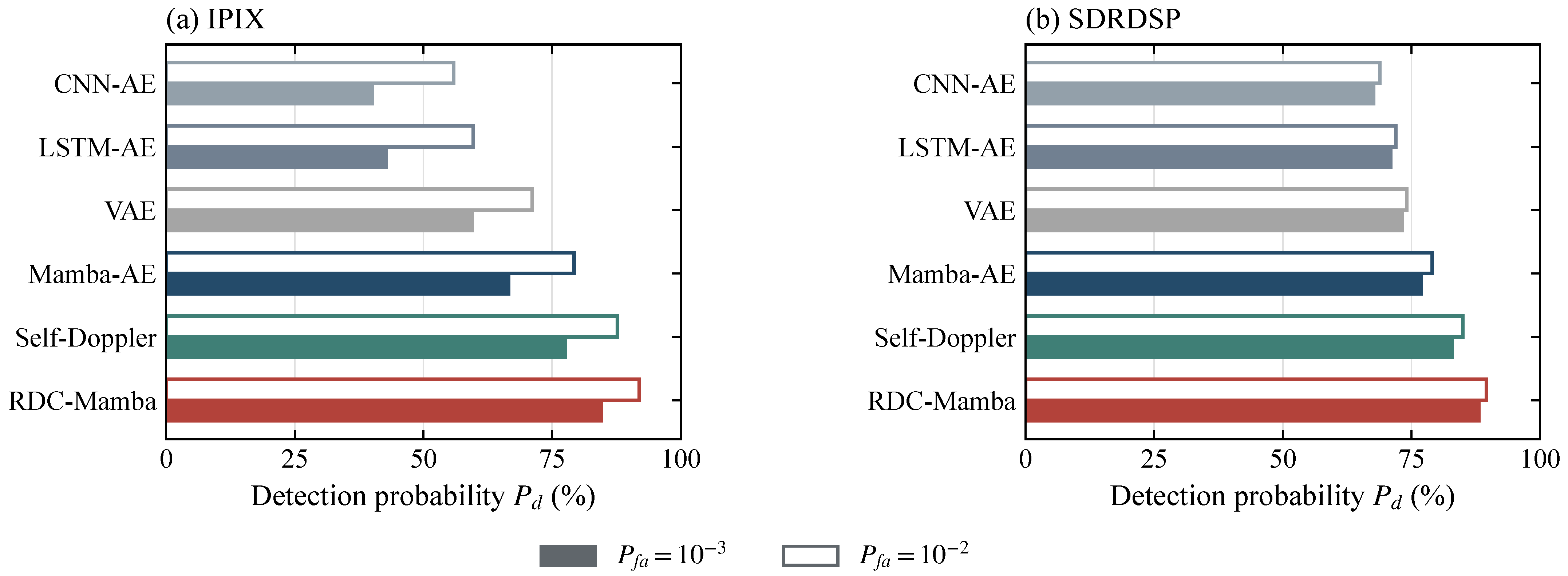
When the false-alarm probability is reduced from to , the detection probability of RDC-Mamba decreases by 7.4 percentage points on IPIX and 1.4 percentage points on SDRDSP. The corresponding decreases for Mamba-AE are 12.7 and 2.1 percentage points. These dataset-dependent changes emphasize the importance of the selected operating point. Figure 8 provides a direct comparison at the two false-alarm probabilities.
Figure 8.
Detection probability at two false-alarm operating points: (a) IPIX; (b) SDRDSP.
As shown in Figure 8, paired bars compare the six autoencoder or generative models at and . Filled bars denote and outlined bars denote , making it possible to compare both the effect of tightening the false-alarm constraint within a method and the ranking of methods under the same constraint. The differences between operating points are generally larger on IPIX than on SDRDSP, reflecting sensitivity to the background represented by each dataset. The bar plot complements Table 3 and the full ROC curves.
The CUT-only Mamba-AE improves on CNN-AE and LSTM-AE on IPIX (AUC 0.988 versus 0.977 and 0.979; 66.6% versus 40.2% and 42.8% at ). Reference conditioning further raises to 84.6% on IPIX and from 77.0% to 88.2% on SDRDSP. These comparisons separate temporal state-space modeling from the additional contribution of reference conditioning.
The comparison can be interpreted in terms of the source of conditioning information. Mamba-AE models CUT temporal dynamics directly, so changes in the local spectrum can increase the reconstruction error of normal clutter. Self-Doppler Mamba conditions on the CUT spectrum, which may contain target information when a target is present. RDC-Mamba instead extracts the condition from neighboring reference cells and incorporates it into state updating to distinguish background changes from local CUT anomalies. The role of reference conditioning therefore involves its information source, normal-echo reconstruction, and anomalous residuals. Detection metrics and the state-modulation mechanism provide complementary levels of analysis.
4.6. Component Configuration Comparisons
Table 4 compares removed modulation branches, alternative condition-fusion schemes, and different condition sources against the full RDC-Mamba configuration. Removing g retains the and B modulation branches; removing and B retains only gate modulation; and removing B and g retains only step-size modulation. Condition concatenation, CUT-derived conditioning, and unconditional modeling form separate controls. Each row represents an independent configuration rather than a sequence in which components are added progressively.
Table 4.
AUC for the component configurations. Differences are relative to the full RDC-Mamba configuration and are expressed in percentage points. A check mark indicates an enabled component; a dash indicates an absent or inapplicable component. Fusion denotes adaptive bilateral fusion, and Concat. denotes concatenation.
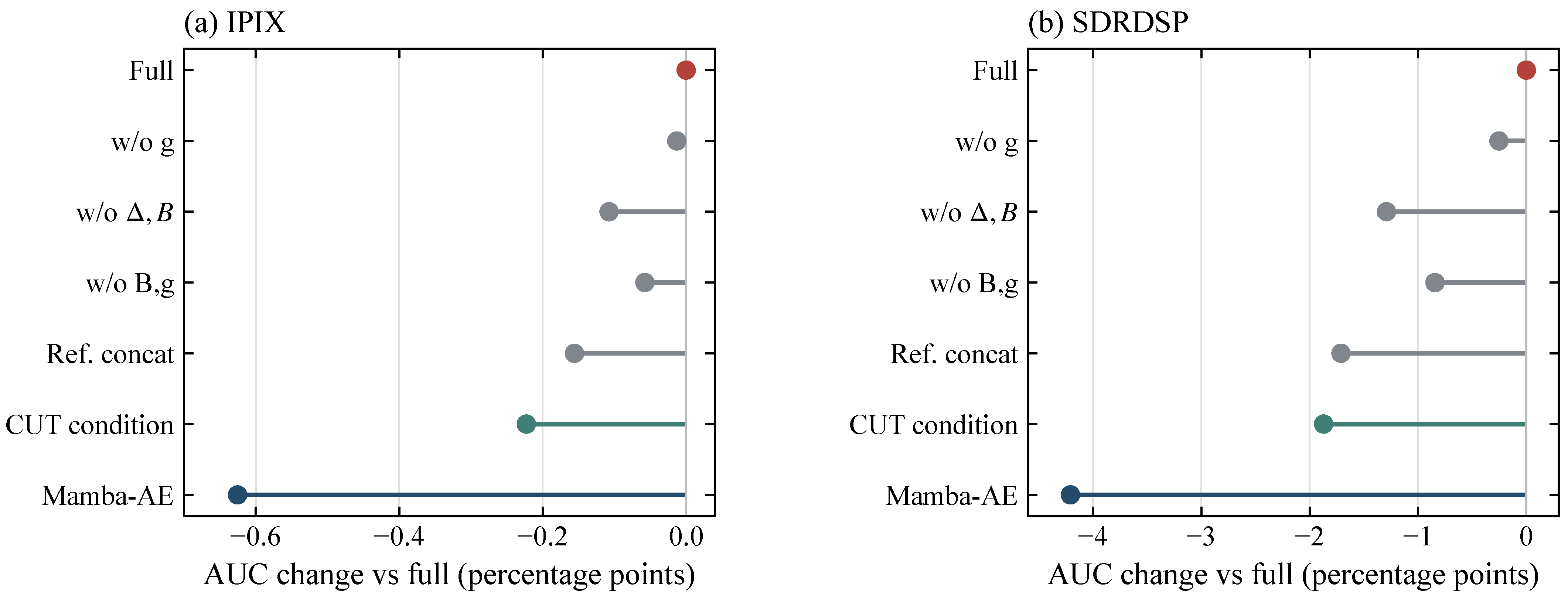
The full configuration has AUC values of 0.994 and 0.997 on IPIX and SDRDSP, respectively. Table 4 reports each AUC and its difference from the full model, calculated before rounding and expressed in percentage points. The full RDC-Mamba configuration has the highest AUC on both datasets. On SDRDSP, removing step-size and input-mapping modulation produces a larger reduction than removing the output gate alone.
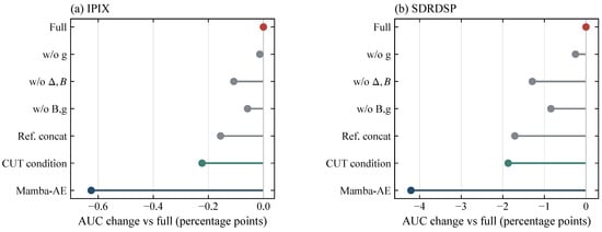
Figure 9 displays the AUC differences relative to the full model around a zero baseline. Both panels use percentage points, with axis ranges chosen to show the smaller changes on IPIX and the larger changes on SDRDSP. The unconditional model shows the largest decrease. Condition concatenation and CUT-derived conditioning also perform below the full configuration, indicating the value of combining reference conditioning with internal state modulation in this comparison.
Figure 9.
AUC differences relative to the full RDC-Mamba configuration. (a) IPIX; (b) SDRDSP. Differences are expressed in percentage points. Red denotes the full configuration, gray denotes reference-conditioned ablations and the concatenation control, green denotes CUT conditioning, and blue denotes the unconditional Mamba-AE.
4.7. Cross-Scenario Comparison and Mechanism Visualization
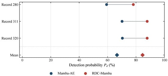
Figure 10 compares the detection probabilities of the three IPIX records using paired points at the low-false-alarm operating point. Diamonds denote the equally weighted means corresponding to Table 3. For records 280, 311, and 320, the detection probabilities of RDC-Mamba are 78.1%, 87.9%, and 87.9%, respectively, compared with 59.3%, 70.2%, and 70.4% for Mamba-AE. RDC-Mamba has higher values for all three records, with a maximum between-record difference of 9.8 percentage points. Its improvements over Mamba-AE are 18.8, 17.7, and 17.5 percentage points, showing that the aggregate advantage is not contributed by a single record alone.
Figure 10.
Record-level IPIX detection probabilities at . Blue and red circles denote record-level results for Mamba-AE and RDC-Mamba, respectively. Diamonds denote the corresponding equally weighted means, and gray lines connect paired results for the same record.
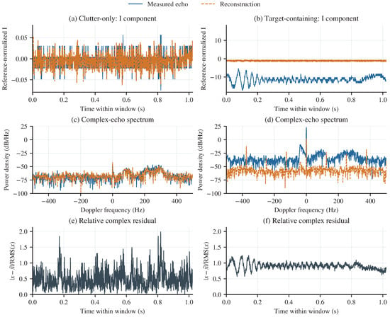
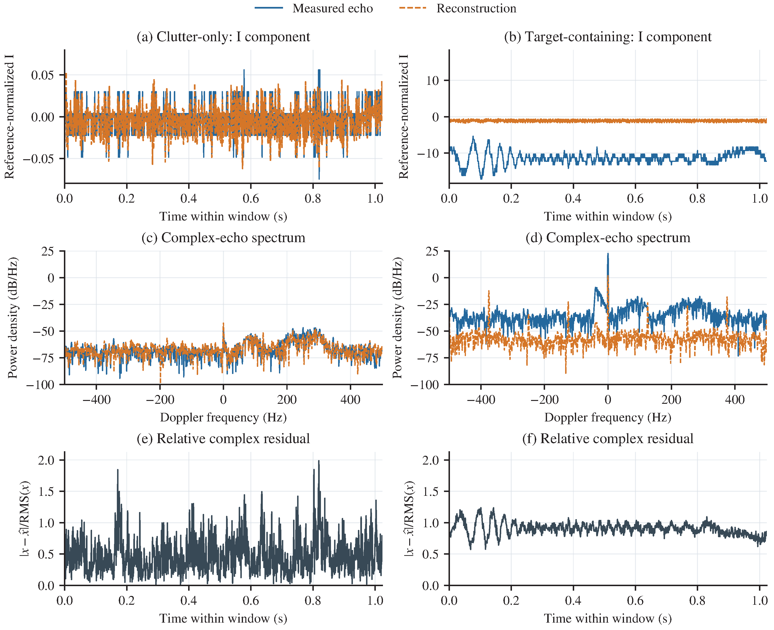
Figure 11 compares measurements and model outputs for two labelled CUT windows from IPIX record 283. The background window (cell 13, 4.096–5.120 s) corresponds to Figure 11a,c,e, and the primary-target-cell window (cell 10, 53.248–54.272 s) to Figure 11b,d,f. With seed 23 fixed, the examples are selected nearest to their class-median scores. Figure 11a,b show measured and reconstructed I components; Figure 11c,d show the corresponding complex-echo power spectra; and Figure 11e,f show the normalized complex-residual magnitude on a shared scale. The target-cell measurement contains clutter and noise as well as the target response. Approximately 97.5% of its squared complex reconstruction error is associated with the window mean; the residual is interpreted as reconstruction mismatch.
Figure 11.
Measured echoes and model outputs for background and target-containing CUT examples. Blue solid and orange dashed curves denote measured and reconstructed echoes, respectively. Black curves in panels (e,f) show the normalized complex-residual magnitude.
4.8. Model Complexity
Table 5 reports latency measurements for the implementations specified in Section 4.3 on a single NVIDIA GeForce RTX 3060. Inputs contain 1024 pulses; batch size is one and precision is float32 without AMP. After 50 warm-up calls, 1000 calls are measured with GPU synchronization. Python 3.9.20, PyTorch 2.5.1+cu121 and CUDA 12.1 are used. SSMs use a pure-PyTorch associative prefix scan, and LSTM uses PyTorch/cuDNN. All latency rows refer to this same benchmark protocol.
Table 5.
Inference latency of the evaluated implementations.
Timing includes model execution and the common multi-resolution reconstruction score on GPU-resident inputs. Reference transforms computed inside the model are included. File I/O, external preprocessing, host-to-device transfers, calibration and observation acquisition are excluded. Synthetic resident tensors are used only for runtime measurement, not for detection evaluation. Means, sample standard deviations and the 50th/95th/99th percentiles are computed from the same 1000 calls.
Under this timing protocol, RDC-Mamba takes 13.522 ms versus 9.680 ms for Mamba-AE, an increase of 39.7%. The additional time is associated with reference spectral encoding, bilateral aggregation and conditional projections. The runtime comparison characterizes the implementations specified in Section 4.3 and includes their full reconstruction-score computation.
Despite the added reference processing, the measured mean window-processing time is 13.522 ms, corresponding to approximately 74 window evaluations per second for the measured GPU-resident computation. At the IPIX PRF of 1 kHz, a 1024-pulse window spans 1.024 s; the mean computation occupies approximately 1.32% of this observation interval. This provides computational headroom for nonoverlapping-window processing and supports further development of an online implementation.
The four-block RDC-Mamba and Mamba-AE architectures contain 0.255/0.209 million parameters and require 1.705/0.505 GFLOPs, corresponding to increases of 22.0% and 237.6%, respectively.
4.9. Supplementary Statistical Summary
Table 6 reports IPIX AUC uncertainty and the Haar reference-transform control. The method order follows Table 3; detection probabilities are expressed as percentages.
Table 6.
IPIX performance and AUC uncertainty for the comparison methods.
For the methods common to Table 3 and Table 6, the IPIX values at coincide; Table 3 reports probabilities, whereas Table 6 reports percentages. AUC summarizes discrimination across ROC thresholds.
The Haar control replaces the STFT in the reference representation with an orthogonal discrete wavelet transform. Low-pass and high-pass filtering with dyadic downsampling provides multiscale reference coefficients. The CUT temporal backbone and temporal/spectral reconstruction-score definition are retained, so the control concerns the reference representation; it does not replace the spectral reconstruction loss with a wavelet loss.
STFT and Haar yield AUC values of 0.9940 and 0.9930, with values of 84.60% and 84.10%, respectively. The small observed differences (0.0010 in AUC and 0.50 percentage points in ) indicate that the reference representation can also use an orthogonal wavelet transform [31]. The overlapping intervals do not by themselves establish equivalence or a significant difference. STFT remains the default because its frequency coordinates provide a direct interpretation of the Doppler background.
5. Conclusions
This paper presented RDC-Mamba for weak target detection in nonstationary sea clutter. The method extracts local time–frequency features from bilateral reference cells outside the guard regions, aggregates them through masked attention and adaptive fusion, and uses the resulting Doppler prior to modulate Mamba step sizes, input mappings, and output gates. By incorporating the prior into internal state updates, the network conditions information writing, retention, and forgetting on the surrounding background and models normal CUT dynamics accordingly.
RDC-Mamba combines clutter-only conditional modeling with temporal and spectral reconstruction errors for anomaly detection. At , its detection probabilities are 84.6% on IPIX and 88.2% on SDRDSP, exceeding Mamba-AE by 18.0 and 11.2 percentage points, respectively. Component and record-level comparisons provide complementary assessments of the framework, while resource comparisons characterize the computational cost of incorporating reference information.
The method depends on local background correlation between the CUT and neighboring reference cells. Abrupt range-dependent clutter changes or widespread contamination by targets, land clutter, or interference can reduce the representativeness of the reference prior. The small number of IPIX range cells and the wider target extent in SDRDSP also require guard-cell selection to account for radar resolution and target scale. Future work will investigate reference-background reliability estimation and anomalous-reference suppression so that the network can reduce its reliance on unreliable priors. Online unsupervised adaptation, polarization diversity, and environmental information will be considered for transfer across radars and sea conditions, alongside streaming state updates and lightweight spectral encoders for real-time detection.
Author Contributions
Conceptualization, Y.C. and H.Z.; methodology, Y.C. and G.L.; software, Y.C. and G.L.; validation, Y.C. and G.L.; formal analysis, M.Z.; investigation, G.L.; data curation, M.Z.; writing—original draft preparation, Y.C.; writing—review and editing, H.Z.; visualization, M.Z.; supervision, G.L.; project administration, H.Z.; funding acquisition, H.Z. All authors have read and agreed to the published version of the manuscript.
Funding
This research was supported by the National Natural Science Foundation of China (Grant No. 91938204, 41527901 and 61701462), Open Project Fund of the State Key Laboratory of Integrated Automation of Process Industries, Northeastern University, Research on Multi-Space Modality Monitoring Methods (SAPI-2024-KFKT-08), the Shandong Provincial Education Department (Grant No. 2024KJN033).
Institutional Review Board Statement
Not applicable.
Informed Consent Statement
Not applicable.
Data Availability Statement
The IPIX radar dataset is publicly available from McMaster University at https://soma.ece.mcmaster.ca/ipix/dartmouth/index.html (accessed on 9 October 2026). The SDRDSP radar dataset is publicly available from the Journal of Radars at https://radars.ac.cn/web/data/getData?dataType=DatasetofRadarDetectingSea (accessed on 9 October 2026). The processed data and plotting scripts are available from the corresponding author upon reasonable request.
Acknowledgments
The authors thank the anonymous reviewers for their insightful comments and constructive suggestions. The authors also thank McMaster University for providing access to the IPIX radar dataset and the team behind the Sea-Detecting Radar Data Sharing Program (SDRDSP) for making the radar datasets publicly available.
Conflicts of Interest
The authors declare no conflicts of interest.
References
- Lanz, P.; Marino, A.; Brinkhoff, T.; Köster, F.; Möller, M. The InflateSAR Campaign: Testing SAR Vessel Detection Systems for Refugee Rubber Inflatables. Remote Sens. 2021, 13, 1487. [Google Scholar] [CrossRef] [Scilit]
- Ward, K.D.; Tough, R.J.A.; Watts, S. Sea Clutter: Scattering, the K Distribution and Radar Performance, 2nd ed.; The Institution of Engineering and Technology: London, UK, 2013. [Google Scholar] [CrossRef] [Scilit]
- Rohling, H. Radar CFAR Thresholding in Clutter and Multiple Target Situations. IEEE Trans. Aerosp. Electron. Syst. 1983, AES-19, 608–621. [Google Scholar] [CrossRef] [Scilit]
- Shui, P.L.; Li, D.C.; Xu, S.W. Tri-Feature-Based Detection of Floating Small Targets in Sea Clutter. IEEE Trans. Aerosp. Electron. Syst. 2014, 50, 1416–1430. [Google Scholar] [CrossRef] [Scilit]
- Guan, J.; Jiang, X.; Liu, N.; Ding, H.; Dong, Y.; Guo, Z. A Small Maritime Target Detection Method Using Nonlinear Dimensionality Reduction and Feature Sample Distance. Remote Sens. 2024, 16, 2901. [Google Scholar] [CrossRef] [Scilit]
- Guo, Z.X.; Bai, X.H.; Li, J.Y.; Shui, P.L.; Su, J.; Wang, L. Small Target Detection in Sea Clutter Using Dominant Clutter Tree Based on Anomaly Detection Framework. Signal Process. 2024, 219, 109399. [Google Scholar] [CrossRef] [Scilit]
- Wang, K.; Wang, Z. A Triple-Channel Network for Maritime Radar Targets Detection Based on Multi-Modal Features. Remote Sens. 2024, 16, 4662. [Google Scholar] [CrossRef] [Scilit]
- Yuan, S.; Gao, H.; Zhang, Z.; Liu, Y. Small target detection in sea clutter based on lightweight multi-dimensional adaptive network. Digit. Signal Process. 2026, 175, 105999. [Google Scholar] [CrossRef] [Scilit]
- Wang, J.; Xiao, T.; Liu, P. Radar Target Detection in Sea Clutter Based on Two-Stage Collaboration. J. Mar. Sci. Eng. 2025, 13, 1556. [Google Scholar] [CrossRef] [Scilit]
- Bai, T.; Tang, J.; Sun, N.; Xu, Y. Radar Target Detection in Sea Clutter via a Detection-Oriented Complex-Valued VAE. Signal Process. 2026, 249, 110758. [Google Scholar] [CrossRef] [Scilit]
- Gu, A.; Goel, K.; Ré, C. Efficiently Modeling Long Sequences with Structured State Spaces. In Proceedings of the International Conference on Learning Representations, Virtual, 25–29 April 2022. [Google Scholar]
- Gu, A.; Dao, T. Mamba: Linear-Time Sequence Modeling with Selective State Spaces. In Proceedings of the Conference on Language Modeling, Philadelphia, PA, USA, 7–9 October 2024. [Google Scholar]
- He, W.; Zhong, Y.; Li, Y.; Wang, J.; Jiang, T. ECMNet: An Efficient CNN–Mamba Network for Maritime Radar Target Detection. In Proceedings of the Machine Learning and Knowledge Engineering for Decision Making; Lecture Notes in Computer Science; Springer: Singapore, 2027; Volume 16754, pp. 291–305. [Google Scholar] [CrossRef] [Scilit]
- Hou, Z.; Ohtsuki, T. Selection, Not Fusion: Radar-Modulated State Space Models for Radar-Camera Depth Estimation. arXiv 2026, arXiv:2605.11840. [Google Scholar] [CrossRef] [Scilit]
- Zhu, Y.; Shen, L.; Su, H.; Li, Z.; Yang, R. Multidimensional Attention–Autocorrelation-Based Small Sea-Surface Target Detection. IEEE Trans. Aerosp. Electron. Syst. 2026, 62, 12130–12145. [Google Scholar] [CrossRef] [Scilit]
- Perez, E.; Strub, F.; de Vries, H.; Dumoulin, V.; Courville, A. FiLM: Visual Reasoning with a General Conditioning Layer. Proc. AAAI Conf. Artif. Intell. 2018, 32, 3942–3951. [Google Scholar] [CrossRef] [Scilit]
- Kim, T.; Kim, J.; Tae, Y.; Park, C.; Choi, J.H.; Choo, J. Reversible Instance Normalization for Accurate Time-Series Forecasting against Distribution Shift. In Proceedings of the International Conference on Learning Representations, Virtual, 25–29 April 2022. [Google Scholar]
- Cohen, L. Time-Frequency Analysis; Prentice Hall PTR: Englewood Cliffs, NJ, USA, 1995. [Google Scholar]
- Zaheer, M.; Kottur, S.; Ravanbakhsh, S.; Póczos, B.; Salakhutdinov, R.; Smola, A.J. Deep Sets. In Proceedings of the Advances in Neural Information Processing Systems, Long Beach, CA, USA, 4–9 December 2017; Volume 30. [Google Scholar]
- Ilse, M.; Tomczak, J.; Welling, M. Attention-Based Deep Multiple Instance Learning. In Proceedings of the 35th International Conference on Machine Learning; PMLR (Proceedings of Machine Learning Research): Brookline, MA, USA, 2018; Volume 80, pp. 2127–2136. [Google Scholar]
- Yamamoto, R.; Song, E.; Kim, J.M. Parallel WaveGAN: A Fast Waveform Generation Model Based on Generative Adversarial Networks with Multi-Resolution Spectrogram. In Proceedings of the ICASSP 2020–2020 IEEE International Conference on Acoustics, Speech and Signal Processing, Barcelona, Spain, 4–8 May 2020; pp. 6199–6203. [Google Scholar] [CrossRef] [Scilit]
- Trabelsi, C.; Bilaniuk, O.; Zhang, Y.; Serdyuk, D.; Subramanian, S.; Santos, J.F.; Mehri, S.; Rostamzadeh, N.; Bengio, Y.; Pal, C.J. Deep Complex Networks. In Proceedings of the International Conference on Learning Representations, Vancouver, BC, Canada, 30 April–3 May 2018. [Google Scholar]
- Drosopoulos, A. Description of the OHGR Database; Technical Note 94-14; Defence Research Establishment Ottawa: Ottawa, ON, Canada, 1994. [Google Scholar]
- McMaster University. IPIX Radar—Dartmouth Database. Available online: https://soma.ece.mcmaster.ca/ipix/dartmouth/index.html (accessed on 9 October 2026).
- Liu, N.; Dong, Y.; Wang, G.; Ding, H.; Huang, Y.; Guan, J.; Chen, X.; He, Y. Sea-Detecting X-Band Radar and Data Acquisition Program. J. Radars 2019, 8, 656–667. [Google Scholar] [CrossRef]
- Liu, N.; Ding, H.; Huang, Y.; Dong, Y.; Wang, G.; Dong, K. Annual Progress of the Sea-Detecting X-Band Radar and Data Acquisition Program. J. Radars 2021, 10, 173–182. [Google Scholar] [CrossRef]
- Journal of Radars. Sea-Detecting Radar Dataset: 2020 Series, Issue 1. SDRDSP Data Release, 2021. Official Batch Title: 2020 Series, Issue 1. Available online: https://radars.ac.cn/web/data/getData?dataType=DatasetofRadarDetectingSea (accessed on 9 October 2026).
- Loshchilov, I.; Hutter, F. Decoupled Weight Decay Regularization. In Proceedings of the International Conference on Learning Representations, New Orleans, LA, USA, 6–9 May 2019. [Google Scholar]
- Fawcett, T. An Introduction to ROC Analysis. Pattern Recognit. Lett. 2006, 27, 861–874. [Google Scholar] [CrossRef] [Scilit]
- Efron, B.; Tibshirani, R.J. An Introduction to the Bootstrap; Chapman & Hall: New York, NY, USA, 1993. [Google Scholar]
- Mallat, S.G. A Theory for Multiresolution Signal Decomposition: The Wavelet Representation. IEEE Trans. Pattern Anal. Mach. Intell. 1989, 11, 674–693. [Google Scholar] [CrossRef] [Scilit]



Disclaimer/Publisher’s Note: The statements, opinions and data contained in all publications are solely those of the individual author(s) and contributor(s) and not of MDPI and/or the editor(s). MDPI and/or the editor(s) disclaim responsibility for any injury to people or property resulting from any ideas, methods, instructions or products referred to in the content. |
© 2026 by the authors. Licensee MDPI, Basel, Switzerland. This article is an open access article distributed under the terms and conditions of the Creative Commons Attribution (CC BY) license.