k-NN Adaptive IPLF–PMBM Underwater Multi-Target Tracking Algorithm

Abstract

The Poisson multi-Bernoulli mixture (PMBM) filter performs well in active sonar tracking, but its standard form assumes a single, globally preset clutter intensity, which matches poorly the range-dependent reverberation of the underwater channel. This paper applies the iterated posterior linearization filter (IPLF) within the PMBM recursion and proposes a k-nearest-neighbor (k-NN) estimator of the local clutter intensity, in which the distance to the k-th neighbor of each measurement sets an adaptive bandwidth and the intensity entering the newborn existence probability comes from the measurements rather than from a preset. In batch form the pairwise distance matrix is formed once per frame, at a cost of 0.14 ms per frame for about ninety measurements. In a power-law clutter scenario, the method reaches a generalized optimal sub-pattern assignment (GOSPA) value of 11.13, which is 22.9% below the standard filter at a preset that underestimates the clutter level, with the difference carried by the false-alarm term. A preset sweep shows that the best fixed value, 11.23, is reached only when the preset is tuned after the fact, and the adaptive method matches it without tuning. The result varies by less than 0.07 over neighbor counts from 8 to 90, and a uniform-clutter control shows that the adaptation neither helps nor harms when the clutter has no spatial structure.

1. Introduction

Based on random finite set (RFS) theory, multi-object tracking algorithms have emerged over the past two decades as an advanced framework for multi-object tracking. Unlike conventional multi-target tracking algorithms, RFS-based approaches directly model the joint distribution of all targets at each time step [1] and propagate it recursively, offering superior tracking accuracy and computational efficiency, with strong performance in dynamic and dense-clutter scenarios. Since RFS-based multi-object tracking algorithms require the evaluation of set integrals, which generally admit no closed-form solution, considerable research effort in recent years has been devoted to seeking tractable RFS approximations. The probability hypothesis density (PHD) filter [2] approximates the RFS posterior by modeling the multi-object distribution as a Poisson point process, thereby avoiding explicit data association and improving computational efficiency. The Multi-target multi-Bernoulli (MMB) filter [3,4], on the other hand, models the multi-object posterior as a multi-Bernoulli process and is better suited to low-clutter, sparse-target scenarios compared to the PHD filter.

The Poisson multi-Bernoulli mixture (PMBM) filter unifies the PHD and MMB filters through a more general RFS formulation and achieves a favorable balance between computational efficiency and tracking accuracy. In 2013, Williams first derived the PMBM filter within the probability generating functional (PGFL) framework [5]. In 2016, García-Fernández et al. derived the filter without relying on PGFLs [6] and established its conjugacy, providing a complete theoretical foundation for its application. The core idea of the PMBM filter is to model undetected targets as a Poisson point process and previously detected targets as a multi-Bernoulli mixture; the union of the two jointly describes the multi-object posterior distribution. Compared to other RFS-based filters, the PMBM filter achieves higher tracking accuracy and is particularly effective in dense-clutter and dynamic scenarios [7].

At INEC 2020, Miao et al. first applied the PMBM filter to measurement-level fusion of maritime radar and automatic identification system (AIS) data for multi-object detection and tracking of autonomous surface vessels [8], representing an early exploration of PMBM in a real sensor fusion context. In 2022, Lee et al. introduced the PMBM filter to centralized multi-sensor fusion for autonomous driving [9], proposing a weighted fusion strategy based on sensor uncertainty. In the same year, Wright et al. integrated the BELLHOP ray-tracing model into the PMBM filter [10], combining a realistic underwater acoustic propagation model with PMBM for the first time. In 2023, Zhu, Xie et al. proposed a robust PMBM filter based on Student’s t-distribution [11], deriving a closed-form solution via variational Bayesian methods and demonstrating significant robustness to heavy-tailed process and measurement noise in radar applications. Also in 2023, Zhang applied the PMBM filter to multi-static autonomous underwater vehicle (AUV) systems with unknown detection parameters [12], handling port-starboard ambiguity, clutter, and missed detections simultaneously, and validating the transferability of PMBM to underwater sonar. In 2024, Deleskog et al. applied PMBM to aircraft target tracking in multi-static passive bistatic radar [13], providing the first systematic validation of PMBM for passive radar.

The birth model of the PMBM filter is typically configured with a large covariance to monitor a larger surveillance region, which necessitates certain approximations in nonlinear scenarios. However, a large initial covariance renders the posterior covariance matrix highly sensitive to estimation errors: conventional extended Kalman filter (EKF) and unscented Kalman filter (UKF) [14,15] algorithms cannot accurately estimate the posterior covariance matrix and are thus prone to failure in updating the existence probability of newborn targets. In 2022, García-Fernández et al. first combined the iterated posterior linearization filter (IPLF) [16] with the PMBM filter, yielding the IPLF–PMBM filter [17]. As a filtering approach that fully exploits posterior information, the IPLF achieves accurate estimation of the posterior covariance matrix and is particularly well suited as a tracking filter in nonlinear scenarios.

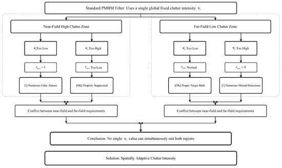
The standard IPLF–PMBM filter assumes that clutter is uniformly distributed over the surveillance region and employs a single, globally preset clutter intensity. This assumption is approximately valid in radar or airborne early-warning scenarios. However, in active sonar tracking, clutter exhibits a markedly non-uniform distribution along the range dimension due to the physical mechanisms of volume reverberation and interface reverberation: clutter is intense at short ranges, where the clutter density is far higher than in the far field. When the preset clutter intensity is too low, the filter underestimates the clutter weight of newborn Bernoulli components in Equation (6), generating a large number of false tracks. Conversely, when the clutter intensity is too high, the existence probability of true targets in the low-clutter far field is excessively underestimated, leading to a high rate of missed detections. Owing to the spatial non-uniformity, a single global intensity cannot serve the near and far fields equally well.

To address this problem, this paper proposes a k-NN adaptive IPLF–PMBM algorithm—a local clutter density estimation method based on k-nearest neighbor [18] adaptive bandwidth. The key idea is as follows: for each measurement, the local distance to its k-th nearest neighbor is used as an adaptive bandwidth in place of the global preset, thereby estimating the local clutter intensity in real time. In the high-clutter near field, the adaptive bandwidth automatically shrinks, increasing the estimated clutter intensity and suppressing false alarms. In the low-clutter far field, the adaptive bandwidth automatically expands, decreasing the estimated clutter intensity and reducing missed detections.

Estimating clutter from the measurements themselves is not new. Clutter-map methods divide the surveillance region into cells and estimate the density in each cell from counts accumulated over several scans [19]. They need no model, but the cell size and the memory length must be chosen, and the estimate is piecewise constant, so a gradient inside a cell is lost. Parametric methods model the clutter as a non-homogeneous Poisson process with a Gaussian-mixture intensity and estimate its parameters jointly with a PHD filter [20]. The result is smooth, but it assumes a functional form and carries its parameters through the recursion. Nonparametric density estimation avoids that assumption: the k-nearest-neighbor estimator of Loftsgaarden and Quesenberry [21] and the kernel estimators surveyed by Silverman [18] return a local density directly from the sample. The closest precedent is the spatial clutter measurement density estimator, which estimates the local density as the neighbor order divided by the volume of the hypersphere that reaches that neighbor [19]. Its use has been confined to the association probabilities of PDA-type trackers, and the volume is Euclidean. The estimator proposed here shares that neighbor-order form. The differences are the measure in which the volume is computed, which makes the estimate directly comparable with the global intensity, and the stage at which it enters the filter.

The contributions of this paper are threefold. First, a k-nearest-neighbor estimator of the local clutter intensity is introduced into the birth stage of the PMBM filter, replacing the global preset with a bandwidth that follows the local measurement density. The estimator follows from a method-of-moments argument, adds no parameter beyond the neighbor count, and is implemented in batch form at a cost of 0.14 ms per frame. Second, the estimator is combined with the IPLF update and compared with the standard IPLF–PMBM, UKF-PMBM and EKF-PMBM filters on a range-dependent clutter profile under common realizations, with the error decomposed into localization, missed-detection and false-alarm terms so that the effect of the adaptation can be attributed. Third, the conditions under which the adaptation helps are delimited: a preset sweep, a neighbor-count ablation and a uniform-clutter control show that the gain appears where the clutter is spatially non-uniform, that it is insensitive to the neighbor count over a wide range, and that it vanishes when the clutter is uniform.

The remainder of the paper is organized as follows. Section 2 reviews the standard IPLF–PMBM filter and identifies the limitation of a globally preset clutter intensity. Section 3 develops the local estimator, its batch implementation and the choice of the neighbor count. Section 4 reports the simulation study, covering the four-method comparison, the preset sweep, the neighbor-count ablation, the update-model comparison, the uniform-clutter control and the timing. Section 5 discusses the results and their limitations, and Section 6 concludes the paper.

2. Standard IPLF–PMBM Algorithm and Its Limitations

2.1. Target Model

The target is assumed to be a point target moving in a two-dimensional Cartesian coordinate system. At time step k, the target state is x_k = [x_k, ẋ_k, y_k, ẏ_k]^T, where x_k and y_k denote the horizontal and vertical coordinates of the target, respectively; ẋ_k and ẏ_k are the corresponding velocity components; and the superscript T denotes the transpose. The target motion model adopts the constant velocity (CV) model [22], whose motion equation is:

$$X_{k+1}=F{X}_k+w_k,w_k~\mathcal{N}\left(0,Q\right)$$

(1)

where F = [1, 1, 0, 0; 0, 1, 0, 0; 0, 0, 1, 1; 0, 0, 0, 1] is the state transition matrix; w_k ~ $\mathcal{N}$(0, Q) is the process noise, which obeys a zero-mean Gaussian distribution; and Q is the process noise covariance matrix, derived from the piecewise constant white acceleration model:

$$Q={\sigma }_w^2{I}_2\otimes \left[\begin{array}{cc}{T}^3/3& T^2/2\\ T^2/2& T\end{array}\right]$$

(2)

where ${\sigma }_w^2{I}_2$ is the process noise intensity (${\sigma }_w^2{I}_2$ = 0.8 is adopted in this paper). At time step k + 1, the target measurement is:

$$Z_{k+1}=h\left(X_{k+1}\right)+v_{k+1},v_{k+1}~\mathcal{N}\left(0,R\right)$$

(3)

where z_k+1 = [r_k+1, θ_k+1]^T; v_k+1 is the measurement noise, with $R=diag({\sigma }_r^2,{{\sigma }_{\theta }}^2)$, where ${\sigma }_r^2$ is the range measurement noise variance and ${{\sigma }_{\theta }}^2$ is the bearing measurement noise variance; and $h\left(\cdot \right)$ is the measurement function, whose coordinate transformation is given by:

$$\left\{\begin{array}{c}{r}_{k+1}=\sqrt{x_{k+1}^2+y_{k+1}^2}\\ {\theta }_{k+1}=ta{n}^{-1}\left({\displaystyle \frac{y_{k+1}}{x_{k+1}}}\right)\end{array}\right.$$

2.2. Conjugate Structure of the PMBM Filter

The PMBM prior distribution is a conjugate prior: if the prior at time k − 1 is of PMBM form, then under the standard multi-target measurement model and after Bayesian recursion, the posterior at time k retains the PMBM form. This property enables the PMBM filter to realize rigorous Bayesian recursion in closed form without resorting to particle approximations.

The PMBM filter decomposes the multi-target state set X into two mutually exclusive subsets $X=Y\uplus W$, where Y denotes the set of potential (undetected) targets and W denotes the set of already-detected targets. The posterior density is the convolution of the two densities:

$$f\left(X\right)={\sum }_{Y\uplus W=X}\underset{\mathrm{PPP}: \mathrm{potential} \mathrm{targets}}{\underbrace{e^{-⟨\lambda ;1⟩}{\displaystyle \prod _{x\in Y}\lambda }(x)}}\cdot \underset{\mathrm{MBM}: \mathrm{detected} \mathrm{targets}}{\underbrace{{\displaystyle {\displaystyle \sum _{h=1}^H}{w}_h}{\displaystyle {\displaystyle \prod _{i=1}^{N_b}}{f}_h^i}(X^i)}}$$

(4)

In Equation (4), the PPP (Poisson point process) is parameterized by the intensity function λ(x) as a sufficient statistic, with the number of targets obeying a Poisson distribution with mean ∫λ(x)dx, and the individual target states being mutually independent. The MBM (multi-Bernoulli mixture) describes already-detected targets and the data association history using H weighted multi-Bernoulli distributions; each hypothesis h corresponds to a possible global association, with weight w_h proportional to the posterior probability. The quantity N_b denotes the number of Bernoulli components under hypothesis h, where each Bernoulli component f_hⁱ(Xⁱ) is parameterized by existence probability $r_h^i\in [0,1]$ and spatial distribution $p_h^i(x)$.

In the prediction step of the PMBM filter, let the target survival probability be P_S. Assuming that target motion obeys a Markov process, and that the transition density is π(x₊|x), the PPP intensity prediction equation is:

$${\lambda }_{+}\left(x_{+}\right)={\lambda }_{birth}\left(x_{+}\right)+P_S{\displaystyle \int \pi }\left(x_{+}|x\right)\lambda \left(x\right)dx$$

(5)

where ${\lambda }_{birth}\left(x_{+}\right)$ denotes the newborn target intensity.

In the update step, let the target detection probability be P_D. PPP components that are misdetected are retained within the PPP, whereas detected components are appended to the existing MBM as newborn Bernoulli components. Existing MBM Bernoulli components generate a detection hypothesis and a misdetection hypothesis for each measurement. The focus of this paper is the generation of newborn Bernoulli components. For a measurement $z^j$, all PPP components that fall within the validation gate are merged, after the update step, into a single newborn Bernoulli component whose existence probability is:

$$r_{new}^j={\displaystyle \frac{C_j}{C_j+\kappa }}$$

(6)

where $C_j={\sum }_i{w}_p^i{P}_D{\mathcal{l}}_i(z^j)$ denotes the weighted likelihood sum of all PPP components evaluated at $z^j$, representing the likelihood that “the measurement originates from a real target”, and κ denotes the clutter intensity, representing the likelihood that “the measurement originates from clutter”.

The clutter intensity in Equation (6) is a density with respect to the range–bearing measurement space. It counts clutter per unit range and per unit bearing, so the expected number of clutter points inside any region is the integral of the intensity over that region in the measure $\mathrm{d}r\mathrm{d}\theta$. The measure of the whole surveillance region is $V=\Theta R_{\max }$, where $\Theta$ is the angular span in radians and R_max is the maximum range. The standard filter presets one global intensity κ₀, and the presetting is normally done through the product κ₀V, which is simply the expected number of clutter points per frame. Every intensity reported in this paper is expressed in this same measure.

When $C_j\gg \kappa$, we have $r_{new}^j\to 1$, in which case a newborn target is confirmed; when $C_j\ll \kappa$, we have $r_{new}^j\to 0$, in which case the measurement is confirmed as clutter. Hence, the value of κ directly determines the false-alarm and missed-detection probabilities of newborn Bernoulli components—when κ is too small, $r_{new}$ is generally elevated, increasing false alarms; when κ is too large, $r_{new}$ is generally depressed, increasing missed detections. This conflict is difficult to reconciled by a global constant κ₀ in spatially non-uniform clutter scenarios, and constitutes the central research problem of this paper.

2.3. IPLF Nonlinear Update

In the IPLF–PMBM algorithm, the IPLF is employed to update the posterior mean and covariance of the target state. The filter iteratively optimizes the choice of linearization parameters by approximately minimizing the Kullback–Leibler divergence. Since newborn targets in the PMBM algorithm are typically assigned a large covariance, the predicted measurement distribution (e.g., position uncertainty) becomes excessively diffuse, which makes accurate estimation of the posterior distribution especially critical to avoid a large number of missed detections. Owing to its robust adaptability to covariance matrix uncertainty, the IPLF is particularly well-suited for PMBM-based filters.

Let the prior of the component to be updated be $\mathcal{N}\left(x;m,P\right)$, let the actual measurement be $z$, and let the number of IPLF iterations be $N_{it}$. The algorithm flow [16] is as follows:

Initialization:

The linearization point of the first iteration is set to the prior, so that $m_0=m$ and P₀ = P. The prior $\mathcal{N}(x;m,P)$ is held fixed throughout the iterations and is used as the predicted distribution in every Kalman update. What changes from one iteration to the next is the linearization point. Both its mean and its covariance are replaced by those of the posterior obtained in the previous iteration.

Iteration t (t = 0, 1, …, N − 1):

(1)

Generate sigma points: Taking the current linearization point $\mathcal{N}(x;m_t,P_t)$ as the reference, generate 2n_x + 1 sigma points ${\{{\chi }_t^{\left(i\right)}\}}_{i=0}^{2n_x}$ according to the UKF method [14], where n_x denotes the state dimension.

(2)

Measurement propagation: Propagate all sigma points through the nonlinear measurement function (Equation (3) to the measurement space, obtaining ${\mathcal{Z}}_t^{\left(i\right)}=h({\chi }_t^{\left(i\right)})$.

(3)

Statistical linear regression: For the propagated sigma point set, compute the predicted measurement mean ẑ_t, the measurement covariance S_t, and the cross-covariance C_t. From these quantities, construct the equivalent linear model $z\approx A_{t}x+b_t+e_t$, where $A_t=C_t^T{P}^{-1}$, $b_t\in {ℝ}^2$, and $e_t~\mathcal{N}\left(0,{\mathsf{\Omega }}_t\right)$ with ${\mathsf{\Omega }}_t=S_t-A_{t}P{A}_t^T$.

(4)

Kalman update: Using the original prior $(m,P)$ as the predicted distribution, perform the standard Kalman update step with the equivalent linear model:

$$m_{t+1}=m+C_t{S}_t^{-1}\left(z-{\widehat{z}}_t\right),P_{t+1}=P-C_t{S}_t^{-1}{C}_t^T$$

(7)

(5)

Convergence check: Set $m_{t+1}$ and $P_{t+1}$ to the posterior mean and covariance produced by the Kalman update of step (4), and return to step (1). As the number of iterations increases, the accuracy of the equivalent linear model in the vicinity of the true posterior improves progressively, and the sequence of linearization points approaches a fixed point, which corresponds to the optimal posterior linearization.

In the PMBM framework, the IPLF is applied in all nonlinear measurement update steps. The simulation experiments in this paper adopt a fixed number of iterations $N_{it}$ = 5, which provides a favorable balance between computational accuracy and efficiency.

2.4. Limitation of the Global Fixed Clutter Intensity

The standard PMBM algorithm assumes that clutter is uniformly distributed over the surveillance region and employs a globally fixed clutter intensity κ₀. However, in underwater multi-target tracking scenarios, the true spatial distribution of clutter ${\kappa }_{true}(x)$ can vary by several-fold along the range direction. Figure 1 illustrates this contradiction:

Figure 1. Illustration of the near-field/far-field conflict caused by a global fixed clutter intensity in spatially non-uniform clutter.

To resolve this contradiction, an adaptive clutter intensity estimation algorithm must be employed, allowing κ to vary with the spatial position of z.

3. k-NN Adaptive Clutter Estimation for the IPLF–PMBM Algorithm

3.1. Core Idea

The core idea of this paper is to introduce the k-NN method from nonparametric density estimation into the Bernoulli birth stage of the PMBM filter. For each measurement z^j, the local distance to its k-th nearest neighbor measurement is employed as an adaptive bandwidth to estimate the local clutter density in real time, replacing the clutter density κ in Equation (6):

$$r_{new}^j={\displaystyle \frac{C_j}{C_j+{\widehat{\kappa }}_{k-NN}\left(z^j\right)}}$$

(8)

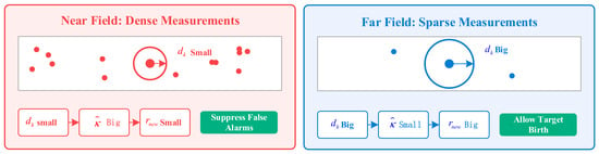
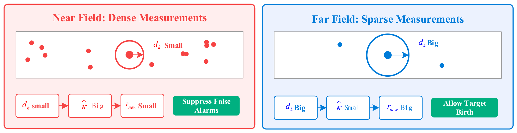
The k-NN estimator possesses intrinsic bandwidth adaptivity: in measurement-dense regions, the distance to the k-th nearest neighbor is small (d_k is small), yielding a small neighborhood measure A(d_k) and hence a high estimated clutter density; in measurement-sparse regions, the distance to the k-th nearest neighbor is large (d_k is large), yielding a large neighborhood measure and hence a low estimated clutter density. This property naturally accommodates the non-uniform clutter distribution characteristic of underwater tracking scenarios.

3.2. Distance Metric in Pseudo-Cartesian Coordinates and k-NN Local Clutter Density Estimation

The measurement z = [r, θ] ^T resides in polar coordinates, where r and θ have different physical dimensions. To measure distances between measurements on a common scale, a pseudo-Cartesian coordinate transformation is adopted:

$$\tilde{x}=r, \tilde{y}={\displaystyle \frac{R_{max}}{\pi }}\cdot \theta$$

(9)

where R_max is the maximum range of the surveillance region, and the term $\tilde{y}$ converts the bearing angle into an equivalent arc length. The distance between two points is defined as the Euclidean distance in pseudo-Cartesian coordinates:

$$d\left(z_a,z_b\right)=\sqrt{{\left(r_a-r_b\right)}^2+{\left({\displaystyle \frac{R_{max}}{\pi }}\left({\theta }_a-{\theta }_b\right)\right)}^2}$$

(10)

For a measurement z^j, let the pseudo-Cartesian distances to the remaining m − 1 measurements, sorted in ascending order, be $d_{(1)}\le d_{(2)}\dots d_{(m-1)}$, with the k-th nearest neighbor distance being $d_k(z^j)=d_{(k)}(z^j)$. The ball centered at z^j with radius d_k(z^j) contains exactly k neighboring measurements, excluding z^j itself. Since the clutter intensity κ is a density with respect to the range–bearing measurement measure $\mathrm{d}r\mathrm{d}\theta$, the neighborhood of z^j must be measured in the same way rather than in physical area. The coordinate transformation of Equation (9) has the constant Jacobian $R_{max}/\pi$, so that $\mathrm{d}r\mathrm{d}\theta =(\pi /R_{max})d\tilde{x}d\tilde{y}$ and the measurement measure of this ball is:

$$A\left(d_k\right)={\displaystyle \frac{{\pi }^2}{R_{max}}}{d_k}^2$$

(11)

Here A(d_k) denotes the neighborhood measure in the range–bearing space and not a physical area. The quantity A is a measure and not an area. It is expressed in the same measure as the clutter intensity, that is, per unit range and per unit bearing, and it follows from the pseudo-Cartesian area of the ball through the constant factor $\pi /R_{\max }$ of Equation (13). The estimate $\widehat{\kappa }$ is therefore obtained in units of inverse meter and inverse radian, which are exactly the units of κ₀, and it can be substituted into Equation (6) with no conversion constant. Because the radian is dimensionless, the same statement can be made with A in meters and $\widehat{\kappa }$ in inverse meters, but the measure $\mathrm{d}r\mathrm{d}\theta$ is the natural choice here since it is the measure in which κ₀ is preset.

Hence, the k-NN estimate of the local clutter density is:

$${\widehat{\kappa }}_{k-NN}\left(z^j\right)={\displaystyle \frac{k}{A\left(d_k\left(z^j\right)\right)}}={\displaystyle \frac{k{R}_{\max }}{{\pi }^2{d}_k^2(z^j)}}$$

(12)

Under the Poisson assumption adopted in Section 2, Equation (12) admits a direct method-of-moments interpretation. For a measurement $z^j$, the k-NN ball of radius d_k(z^j) contains exactly k neighboring measurements by construction, so that the expected number of measurements within the ball, approximately κ(z^j)·A(d_k), equals k; solving for the local intensity yields the estimator in Equation (12). As the number of measurements per scan grows, d_k shrinks and, under mild regularity conditions, $\widehat{\kappa }$(z^j) converges to the underlying intensity of the measurement process. Since target-originated measurements form only a small fraction of the measurement set in the scenarios considered, this intensity is a faithful proxy for the clutter intensity κ(z). Two caveats should be stated explicitly. First, like all k-NN density estimators, $\widehat{\kappa }$ is positively biased, because the reciprocal of the estimated neighborhood measure is convex in that measure, so that its expectation exceeds the reciprocal of the expected measure; this bias is responsible for the modest increase in missed-detection cost reported in Section 4. Second, $\widehat{\kappa }$ estimates the intensity of the whole measurement process rather than of clutter alone; whenever target-originated measurements become a non-negligible share of the measurement set, the estimate is inflated in the immediate vicinity of genuine targets. In the scenarios considered here, at most six target echoes are superimposed on roughly ninety clutter points per scan, so both effects remain small.

Figure 2 provides the adaptive behavior of the k-NN estimator in the near field and the far field, using two representative measurement points in a sector-shaped surveillance region as examples.

Figure 2. Illustration of the k-NN adaptive local clutter density estimation mechanism.

In the near field, measurements are densely distributed; the k-th nearest neighbor distance d_k is small and the corresponding neighborhood measure A(d_k) is small, so the local clutter density estimate $\widehat{\kappa }=k/A(d_k)$ is large. Substituting the larger $\widehat{\kappa }$ into Equation (6) increases the denominator term, thereby reducing the newborn Bernoulli existence probability r_new and effectively suppressing false alarms in the near-field dense clutter region. In the far field, the situation is reversed: measurements are sparsely distributed, d_k is large and the corresponding neighborhood measure is large, so the local clutter estimate is small; the denominator term in Equation (6) decreases and r_new increases, allowing genuine targets to be born normally.

Derivation of the area formula:

In the pseudo-Cartesian plane, the ball of radius d_k centered at a measurement has the area πd_k². This plane, however, is not an isometric image of the range–bearing space. From the Jacobian of the coordinate transformation:

$${\displaystyle \frac{\partial \left(\tilde{x},\tilde{y}\right)}{\partial \left(r,\theta \right)}}=\left|\begin{array}{cc}1& 0\\ 0& R_{max}/\pi \end{array}\right|={\displaystyle \frac{R_{max}}{\pi }}$$

(13)

we obtain $\mathrm{d}\tilde{x}d\tilde{y}=R_{max}/\pi \mathrm{d}r\mathrm{d}\theta$, or equivalently $\mathrm{d}r\mathrm{d}\theta =\pi /R_{max}\mathrm{d}\tilde{x}d\tilde{y}$; Multiplying the pseudo-Cartesian area of the ball by this constant factor yields the neighborhood measure used in Equation (11).

Because the factor is constant over the entire surveillance region, $A(d_k)$ depends only on d_k and on the fixed sensor parameter $R_{max}$, and not on the position of the measurement that anchors the ball. The estimator therefore contains no free constant and requires no mean-range approximation.

For completeness, the corresponding physical area is obtained from the polar area element $\mathrm{dA}=\mathrm{rd}r\mathrm{d}\theta$. The centroid of the ball has $\tilde{x}=r_j$, so the first moment of the ball over the pseudo-Cartesian plane is $r_j\pi d_k^2$,and

$$A_{eff}\left(d_k\right)={\displaystyle \frac{{\pi }^2{r}_j}{R_{max}}}{d_k}^2$$

(14)

which grows linearly with the range r_j of the anchoring measurement. Equation (14) is reported only to make the geometry explicit; it is not used in the estimator, because the clutter intensity in Equation (6) is a density with respect to $\mathrm{d}r\mathrm{d}\theta$ and not with respect to physical area. The two expressions differ by the factor r_j, which is precisely the Jacobian between the physical-area and range–bearing measures.

Boundary effects remain. Near the inner edge of the sector, where d_k exceeds r_j, and at the angular edges, the ball is clipped by the surveillance region, so Equation (11) is only approximate there. Such events are rare, because d_k is small wherever measurements are dense, and their influence on the Monte Carlo averages is negligible.

3.3. Efficient Batch Implementation and Selection of Parameter k

For m measurements, the pairwise distances comprise m(m − 1)/2 distinct entries, so building the full matrix costs O(m²) and sorting it to extract the k-th neighbor of every measurement costs O(m² log m). A pointwise implementation performs the same work one measurement at a time and therefore shares this order. The batch form removes the repetition inside the m independent searches, evaluating the distances once in vectorized form rather than m times in interpreted loops and issuing the sort as a single call on the whole matrix. The gain is therefore a constant factor and not a change of order. With m ≈ 93, the two stages amount to 8.6 × 10³ distance evaluations and 5.7 × 10⁴ comparisons, which differ only by log₂ m ≈ 6.5, so the improvement has to be measured rather than derived. The algorithm pseudocode is as follows (Algorithm 1).

Algorithm 1. k-NN estimation

Input$:\mathrm{Measurement} \mathrm{set} Z=\{[r_1,{\theta }_1],\dots ,[r_m,{\theta }_m]\}$, neighbor count k $\mathrm{Output}: \{{\widehat{\kappa }}_1,\dots ,{\widehat{\kappa }}_m\}$ (1) Pseudo-Cartesian coordinate conversion: $x_j=r_j,y_j=(R_{max}/\pi )\cdot {\theta }_j$  $\forall j=1,\dots ,m$ $\left(2\right) \mathrm{Construct} \mathrm{the} \mathrm{distance} \mathrm{matrix} D\in R^{m\times m}$: $D(i,j)=\mathrm{sqrt}\left(\right(x_i-x_j{)}^2+{(y_i-y_j)}^2)$ $D(i,i)=\infty$ (3) Sort each column and extract the k-th value: $d_k\left(j\right)=\mathrm{sort}(D(:,j))[k]$$\forall j=1,\dots ,m$ (4) Density estimation: ${\widehat{\kappa }}_j=k/(({\pi }^2/R_{max}){d_k}^2(j))$  $\forall j=1,\dots ,m$

The parameter k is the sole tunable parameter of the proposed algorithm, and its statistical interpretation is “the sample size used to estimate the local density”. The choice of k follows a bias-variance trade-off: when k is too small, each estimate uses only a small number of neighboring samples, leading to large sample variance and causing $\widehat{\kappa }$ to fluctuate dramatically between adjacent measurements; when k is too large, d_k approaches the global mean inter-measurement distance, degenerating into a global constant estimate and losing spatial adaptivity. Nonparametric density estimation theory indicates that the asymptotic mean squared error of the k-NN estimator is proportional to k^−4/(d+4) (with d = 2 being the spatial dimension), so the tracking accuracy gain diminishes as k increases. Section 4.4 examines this trade-off empirically. The GOSPA reaches a shallow minimum at k = 20, and no two values between 8 and 90 differ significantly, so the plateau rather than a single value is what the data support.

4. Simulation Analysis

This section evaluates the algorithm through six sets of experiments: a multi-method GOSPA comparison with error component decomposition, a sweep over the global preset κ₀V, an ablation on the neighbor count k, an ablation on the update model, a uniform-clutter scenario at two detection probabilities, and a computational cost comparison.

4.1. Experimental Setup

The surveillance region is a sector of radius Rmax = 1000 m spanning an azimuth of 90°. The sampling interval is T = 1 s and each run covers 41 steps. Six targets move with constant velocity, two in each range band, and their initial states and lifetimes are listed in Table 1.

Table 1. Initial positions, velocities, survival times, and assigned clutter zones of the six simulated targets.

Target	Initial Position (m)	Velocity (m/s)	Survival (s)	Main Clutter Zone
1	(155.6, 155.6)	(−1.77, 1.77)	0–14	near-field
2	(283.7, 221.6)	(1.85, −2.36)	5–25	near-field
3	(500.0, 360.0)	(−2.34, 3.25)	11–37	mid-field
4	(295.1, 579.2)	(3.56, −1.82)	3–29	mid-field
5	(654.2, 424.8)	(−3.35, −2.18)	19–40	far-field
6	(504.8, 720.9)	(−1.15, −1.64)	8–26	far-field

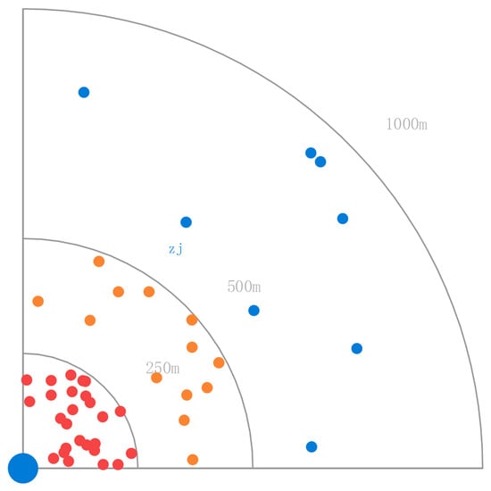
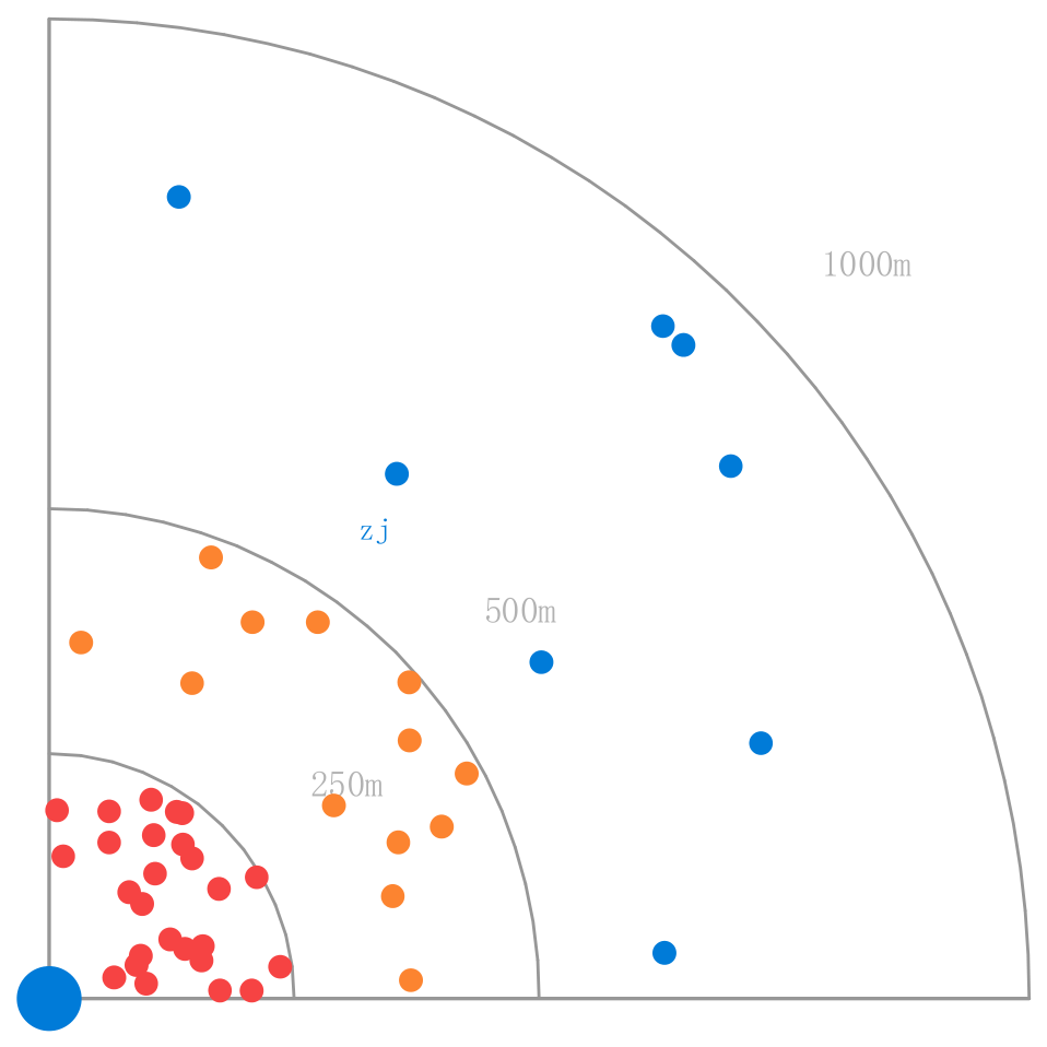
The targets are spread over the three bands so that the spatial adaptivity is exercised across the whole profile, and the clutter intensity falls continuously with range rather than in steps. Clutter is an inhomogeneous Poisson process with intensity $\kappa (r)={\kappa }_{floor}+({\kappa }_{\max }-{\kappa }_{floor}){(1-r/R_{max})}^2$, where κ_floor = 0.008 and κ_max = 0.1559 m⁻¹ rad⁻¹ and the expected count is 90 per frame. Cutting the sector at r = 250 m and r = 500 m leaves 47.9, 26.1 and 16.0 points per frame in the three bands, which sum to 90; the profile is continuous, so the bands are reporting intervals and not steps in the density. A schematic of the surveillance region is shown in Figure 3.

Figure 3. Schematic of the surveillance region.

The count in each band is Poisson with the mean given above, and the positions within a band follow the normalized profile rather than a uniform distribution. The counts of the three bands are in the ratio 3: 1.6: 1. Because the outer band spans twice the range of the others, the corresponding density ratio is about 6: 3.3: 1. Both ratios summarize the continuous profile and are not steps in it.

Target detection probability P_D = 0.9; target survival probability P_S = 0.99. The prediction error covariance is consistent with Equation (1); the measurement error covariance is set to R = diag (1 m², 3 × 10⁻⁴ rad²). The number of IPLF iterations is set to N_it = 5. An elliptical validation gate is adopted, with a confidence level of 99% and gate threshold d² = 9.21. The maximum number of global hypotheses is H_max = 100.

The newborn PPP is not centered on any presumed target position. Its intensity is derived only from the geometry of the surveillance region, an upper bound on the target speed and an assumed number of new targets per frame, and it uses no information about the number, the initial positions or the velocities of the true targets. The region is divided into $N_r\times N_{\theta }=3\times 3$ equal in the range-azimuth measure and equal in width along the bearing direction, and each cell contributes one component. The mean of a component is the geometric center of its cell and the velocity mean is zero. The position covariance follows from a uniform distribution over the cell, which gives ${\sigma }_r=(r_{hi}-r_{lo})/\sqrt{12}$ along the range direction and ${\sigma }_c=r_c\Delta \theta /\sqrt{12}$ across it, and the velocity covariance is ${\sigma }_v=v_{\max }/\sqrt{3}$, from a uniform distribution on [−v_max, v_max]. The parameters are ${\lambda }_{\mathrm{frame}}=0.4$ new targets per frame and v_max = 15 m/s, and every component carries the same weight ${\lambda }_{\mathrm{frame}}/N_r{N}_{\theta }=0.0444$. The intensity of the initial PPP is set equal to the birth intensity, so that the first frame introduces no prior mass of its own. With these settings the three range bands have ${\sigma }_r=166.7$, 69.0 and 53.0 m, and the corresponding lateral standard deviations are ${\sigma }_c=43.6$, 105.3 and 137.3 m.

Pruning thresholds: Bernoulli existence probability: 1 × 10⁻⁵; PPP weight: 1 × 10⁻⁵; MBM global hypothesis weight: 1 × 10⁻⁴. GOSPA parameters: $p=2,c=10,\alpha =2$. Number of Monte Carlo runs N_MC = 100. The i-th realization uses rng(1000i + 9) in Section 4.2, Section 4.3, Section 4.5, Section 4.6 and Section 4.7 and rng(100i + 6) in Section 4.4, shared by all configurations. Test environment: MATLAB 2025b, Intel Ultra X7 358H, 32 GB RAM.

The generalized optimal sub-pattern assignment (GOSPA) metric [23] is adopted to evaluate tracking performance. Let $X=\{x_1,\dots ,x_{|X|}\}$ and $Y=\{y_1,\dots ,y_{|Y|}\}$ be finite subsets of ${ℝ}^N$, where |·| denotes the cardinality of a finite set. The GOSPA metric is defined as:

$$g_p^c\left(X,Y\right)=\left(\underset{\gamma \in \Gamma }{min}\left({\displaystyle \sum _{(i,j)\in \gamma }d}{\left(x_i,y_j\right)}^p\right.\right.{\left.\left.+{\displaystyle \frac{c^p}{2}}\left(\left|X\right|+\left|Y\right|-2\left|\gamma \right|\right)\right)\right)}^{{\displaystyle \frac{1}{p}}}$$

(15)

where $\gamma$ is an assignment set; $\Gamma$ denotes the set of all possible assignment sets between X and Y; c is the cutoff threshold, representing the maximum allowable localization cost; p controls the sensitivity to error and the penalty on outliers, where larger p imposes a heavier penalty. The GOSPA metric simultaneously quantifies the effects of localization accuracy, missed detections, and false alarms, with a smaller g value indicating superior tracking performance.

4.2. Multi-Method GOSPA Comparison and Error Component Decomposition

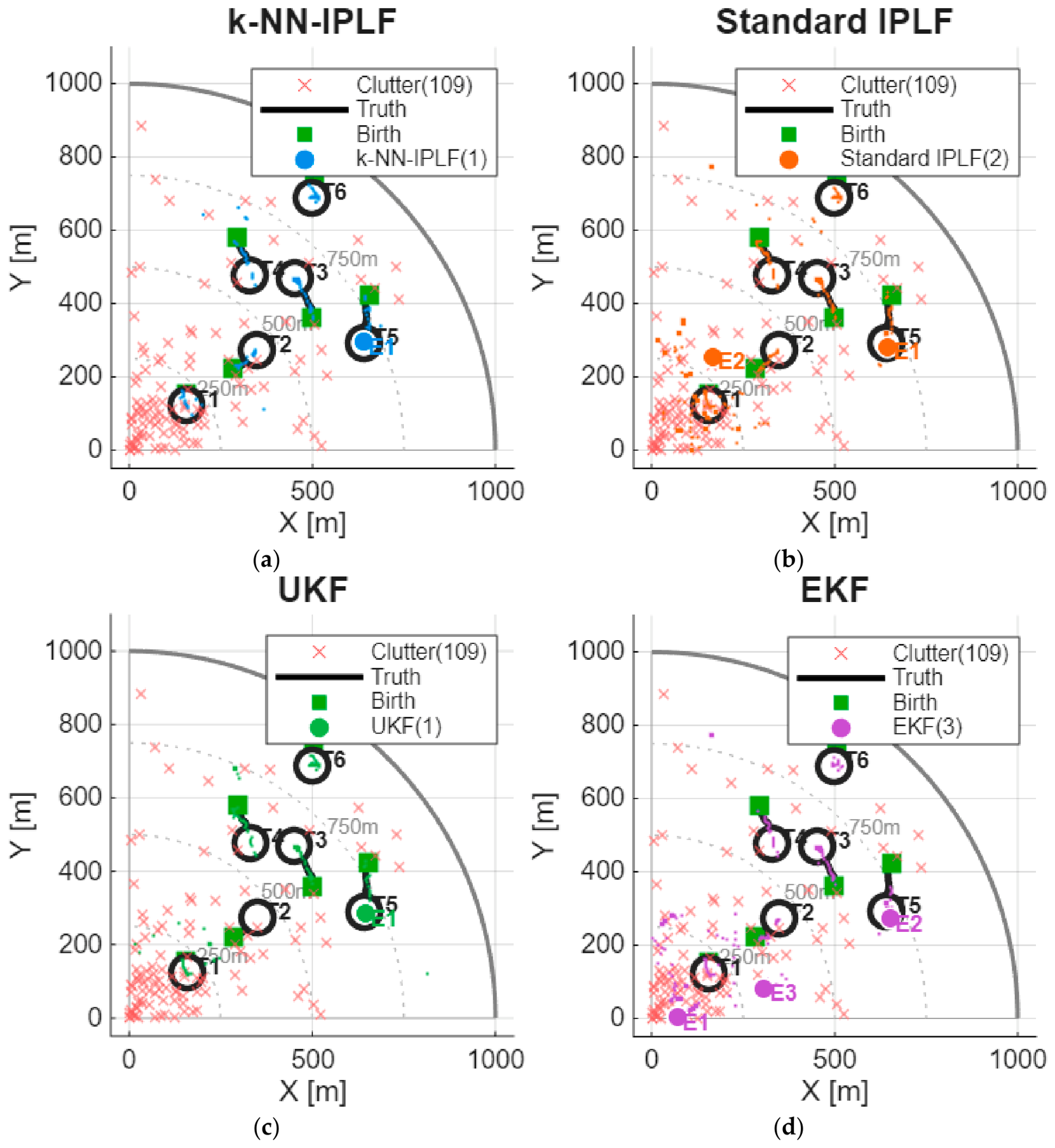
To demonstrate the performance of the k-NN adaptive IPLF–PMBM algorithm, this subsection compares the tracking performance of four algorithms—k-NN adaptive IPLF–PMBM, standard IPLF–PMBM, UKF-PMBM, and EKF-PMBM—in a non-uniform clutter scenario under a low-preset clutter density. The single-trial comparison results are shown above.

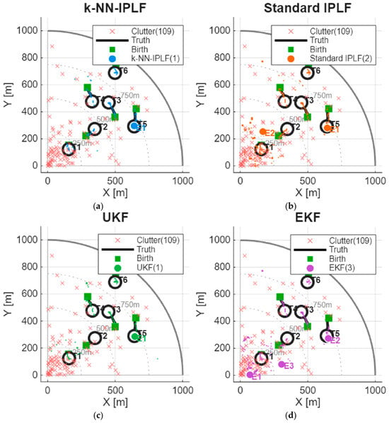
Figure 4 presents the tracking results of the four algorithms in the non-uniform clutter scenario. Taking Figure 4a as an example, the surveillance region is a sector; clutter points are denoted by small red crosses; true trajectories are shown as black lines; current-time target measurements are indicated by hollow circles; current-time target estimates are shown as large filled circles; and small filled circles represent historical estimates. A comparison of the four panels clearly reveals that under a low preset clutter density, the standard IPLF–PMBM, UKF-PMBM, and EKF-PMBM all perform poorly, generating a large number of false alarms, whereas the k-NN adaptive IPLF–PMBM exhibits markedly superior tracking performance.

Figure 4. Single-trial tracking results of four filters under a low clutter preset: (a) k-NN Adaptive; (b) Standard IPLF–PMBM; (c) UKF-PMBM; (d) EKF-PMBM.

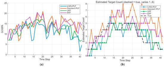
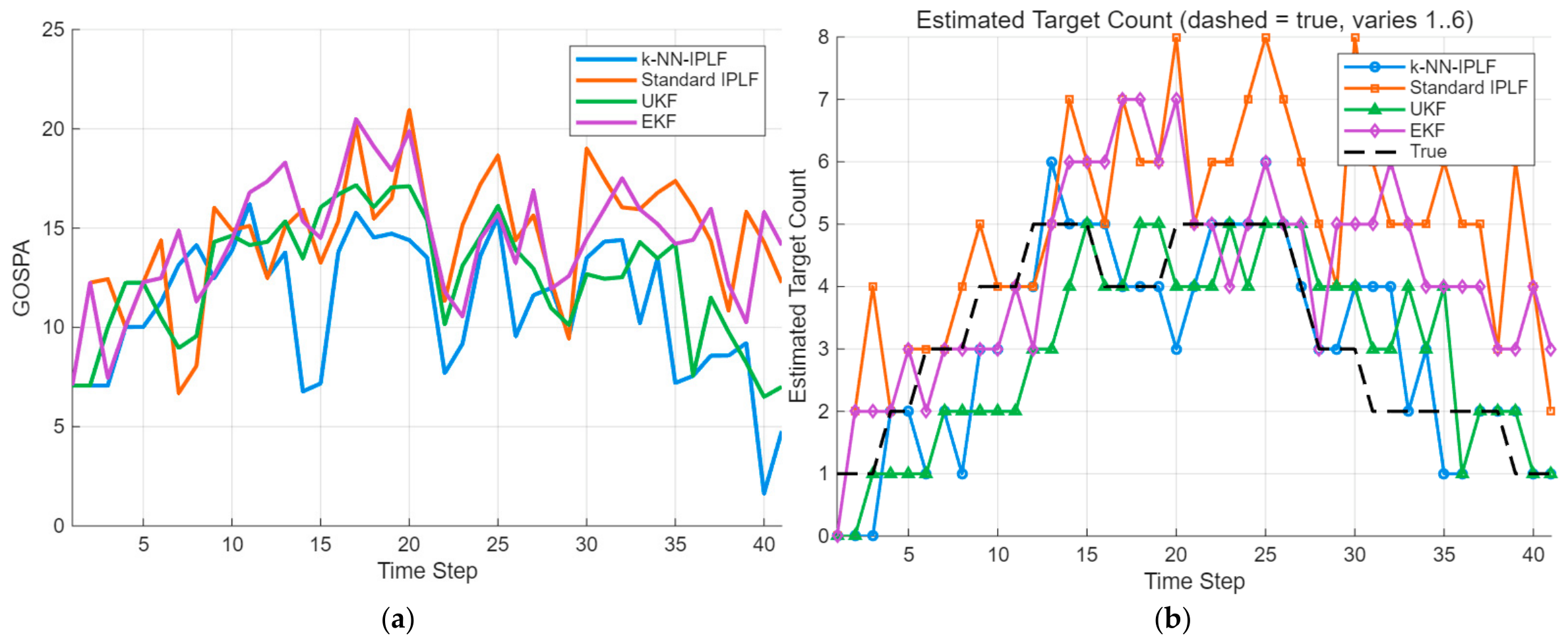
As shown in Figure 5, the k-NN adaptive IPLF–PMBM attains the lowest GOSPA over almost the whole run, with UKF-PMBM next and the standard and EKF-PMBM filters highest. In terms of the estimated target count, the standard and EKF filters settle well above the true count, UKF-PMBM stays close to it, and the k-NN adaptive filter lies slightly below. Among the four filters, the k-NN adaptive IPLF–PMBM gives the best GOSPA and the best control of false tracks, at the cost of a slightly conservative count.

Figure 5. Frame-wise GOSPA and estimated target count comparison for the four filters: (a) multi-method GOSPA performance comparison; (b) multi-method estimated number of targets comparison.

Table 2 presents the results of 100 Monte Carlo simulation trials under this scenario.

Table 2. Monte Carlo GOSPA results with error component decomposition.

Method	Average GOSPA	Std	Localization Cost	Missed-Detection Cost	False-Alarm Cost
k-NN adaptive IPLF–PMBM	11.131	0.640	51.19	53.23	33.60
Standard IPLF–PMBM	14.444	0.710	54.71	42.10	125.33
UKF-PMBM	12.438	0.727	47.18	64.41	57.55
EKF-PMBM	14.623	0.726	46.12	60.32	120.50

According to the Monte Carlo simulation results, the average GOSPA of the k-NN adaptive method is 11.131, representing reductions of 22.9% over the standard IPLF–PMBM, 10.5% over UKF-PMBM, and 23.9% over EKF-PMBM. The error component decomposition shows that localization is not what separates the four filters: the values lie between 46.12 and 54.71 and do not follow the GOSPA ordering, which indicates that the choice of nonlinear filtering strategy has limited influence on the state estimation accuracy for confirmed targets. The term that dominates the difference is the false-alarm cost, which falls from 125.33 for the standard filter and 120.50 for the EKF to 33.60 for the k-NN method, a reduction of about 73%. This reflects the working mechanism of the k-NN adaptive estimator. In the near-field high-clutter region, measurements are densely distributed, the k-th nearest neighbor distance d_k is small, and the local clutter density estimate is correspondingly large; substituting the larger value into the newborn Bernoulli existence probability of Equation (6) increases the denominator term, reduces r_new, and suppresses false tracks. In the far-field low-clutter region, measurements are sparse, d_k is large, and the estimate is small, which favors the birth of genuine targets. The price appears on the missed-detection side, where the k-NN method reports 53.23 against 42.10 for the standard filter, an increase of about 26%. This penalty suggests that the estimator carries a systematic positive bias in absolute magnitude, and the same bias explains why its estimated count of 2.80 stays below the true mean of 3.20 while the standard and EKF filters overshoot to 4.86 and 4.40.

4.3. Expected Clutter Number κ₀V Sweep Experiment

To determine the best performance attainable with a single global value of the standard IPLF–PMBM under a global κ₀, a sweep is performed over the range κ₀V $\in$ {10, 30, 60, 90, 150, 250, 400} (covering a factor of forty from underestimation to overestimation), with N_MC = 100 runs for each κ₀V value. Two references are added to the same table over the same realizations: the k-NN adaptive method, which replaces the preset by the local estimate, and an oracle baseline whose κ is the true spatial clutter intensity at each measurement, so that the estimation error vanishes and only the spatial variation remains.

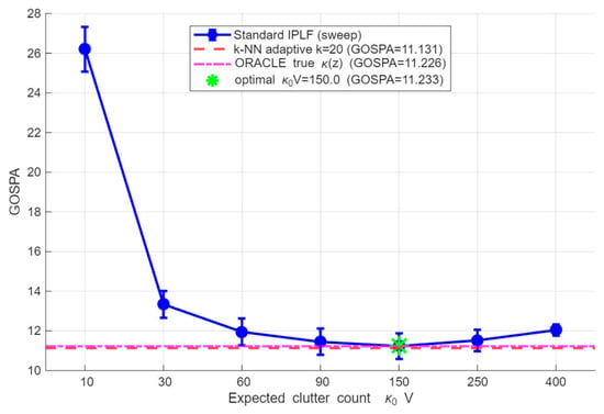
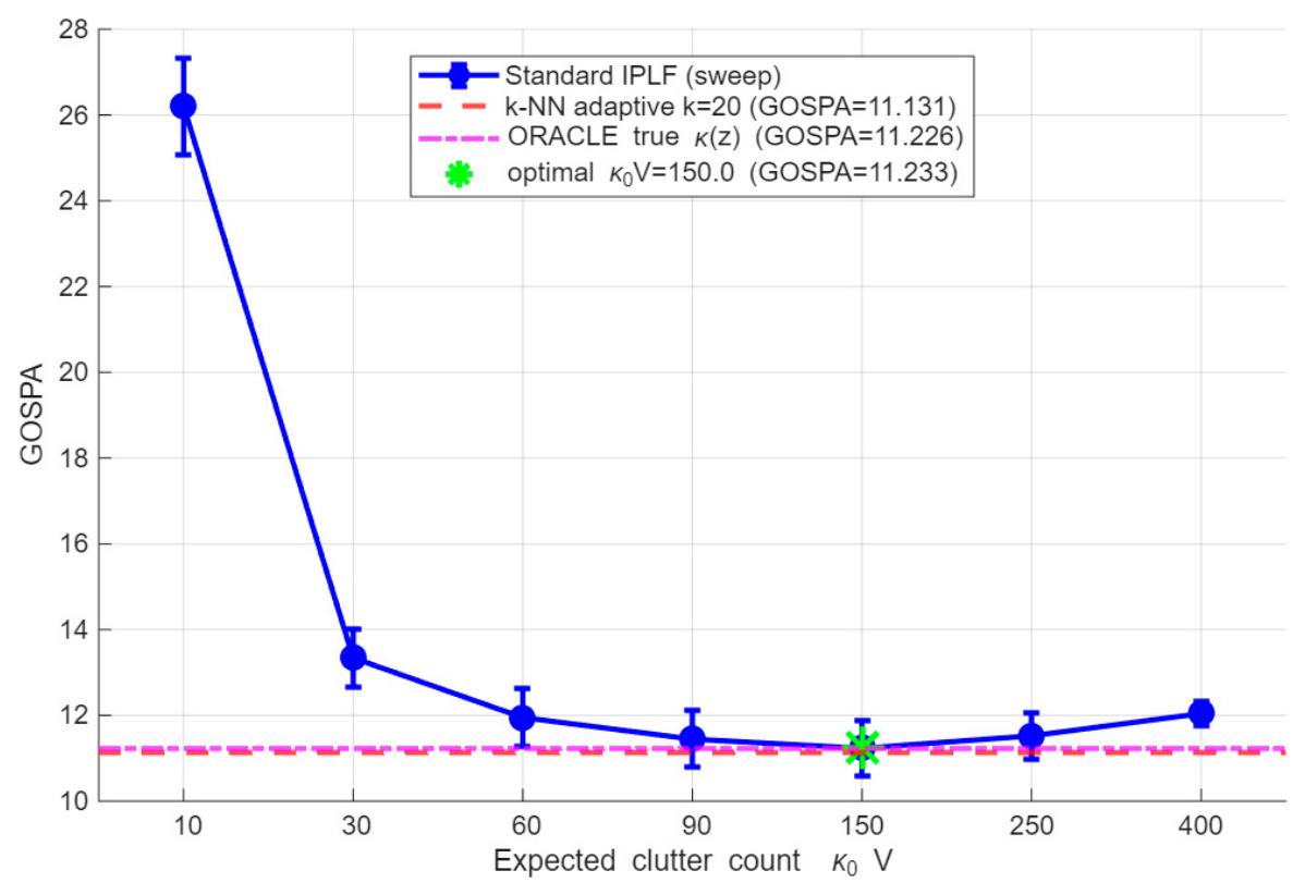
As shown in Figure 6, the GOSPA −κ₀V curve of the standard IPLF–PMBM exhibits a characteristic U-shape. At κ₀V = 10, the GOSPA reaches 26.206 (as detailed in Table 3), which is 2.3 times the optimal value; here, the false-alarm cost dominates absolutely at 619.13, while the missed-detection cost is only 32.85. Under this extreme condition, the severely underestimated κ₀ causes the filter to regard virtually all measurements as potential new targets. As κ₀V increases, the false-alarm cost decreases monotonically from 619.13 to 7.71 at κ₀V = 400—a reduction of approximately 98.8%—while the missed-detection cost increases monotonically from 32.85 to 136.01—an increase of approximately 314.0%. The two error-component curves intersect at around κ₀V = 60 and κ₀V = 90, and the optimal κ₀V is 150, corresponding to a GOSPA of approximately 11.23. At κ₀V = 400, the overestimated clutter intensity suppresses target birth, and the missed-detection cost surpasses the false-alarm cost to become the dominant error source.

Figure 6. κ₀ V sweep experiment results.

Table 3. κ₀ V sweep experiment results.

κ0V	Average GOSPA	Std	Localization Cost	Missed- Detection Cost	False-Alarm Cost
10	26.206	1.127	59.18	32.85	619.13
30	13.340	0.686	53.46	44.83	92.87
60	11.949	0.681	50.90	50.23	55.27
90	11.446	0.664	48.39	56.66	39.91
150	11.233	0.642	42.96	69.10	27.18
250	11.523	0.540	33.79	92.34	19.98
400	12.044	0.300	12.31	136.01	7.71
k-NN	11.131	0.640	51.19	53.23	33.60
Oracle, true κ	11.226	0.699	51.39	51.73	37.18

The GOSPA of the k-NN adaptive method is 11.131. This method uses only the locally estimated ${\widehat{\kappa }}_{k-NN}$ and ignores the global preset value; it is not only completely unaffected by the choice of κ₀V, but also marginally outperforms the standard method under optimal tuning. The oracle reaches 11.226, which is not below the best single constant of 11.233 (paired difference −0.007, t = −0.18), because the optimum at κ₀V = 150 already sits at 1.67 times the true total clutter expectation of 90 rather than at it: a tuned constant absorbs the spatial mismatch by over-suppression, which leaves the true intensity nothing to recover. The k-NN estimate lies 0.094 below the oracle (t = −2.87), with a standard deviation of 0.640 against 0.642 for the best constant. Its neighborhood is truncated by the sector boundary in the far field, which biases it high there, so the missed-detection cost rises from 51.73 to 53.23 while the false-alarm cost falls from 37.18 to 33.60. The advantage thus reflects the direction of the residual error rather than its size, and the oracle is a reference for the spatial variation of the clutter, not a strict bound. However, this observation is scenario-specific: variations in clutter non-uniformity, target count, and spatial distribution may all shift the position of the optimum. In the face of complex and variable underwater acoustic tracking scenarios, this finding should not be generalized as a universal calibration rule. Within the scenarios considered, the k-NN method removes the need for such heuristic strategies. Whether this advantage persists in more realistic environments can only be established with propagation-model-based or recorded sonar data, which we regard as an important next step. That a constant 1.67 times the true mean outperforms the true intensity is a property of the objective rather than of the estimator. With c = 10 m, p = 2 and about ninety clutter points per frame, the GOSPA rewards under-reporting the cardinality, so an unbiased intensity is penalized for its accuracy. The k-NN estimate lies below the oracle only because its far-field bias pushes it in the same direction. We therefore do not read the gap as evidence that the estimator beats the oracle, and we record it as a limitation.

4.4. Ablation Study on the Neighbor Count k

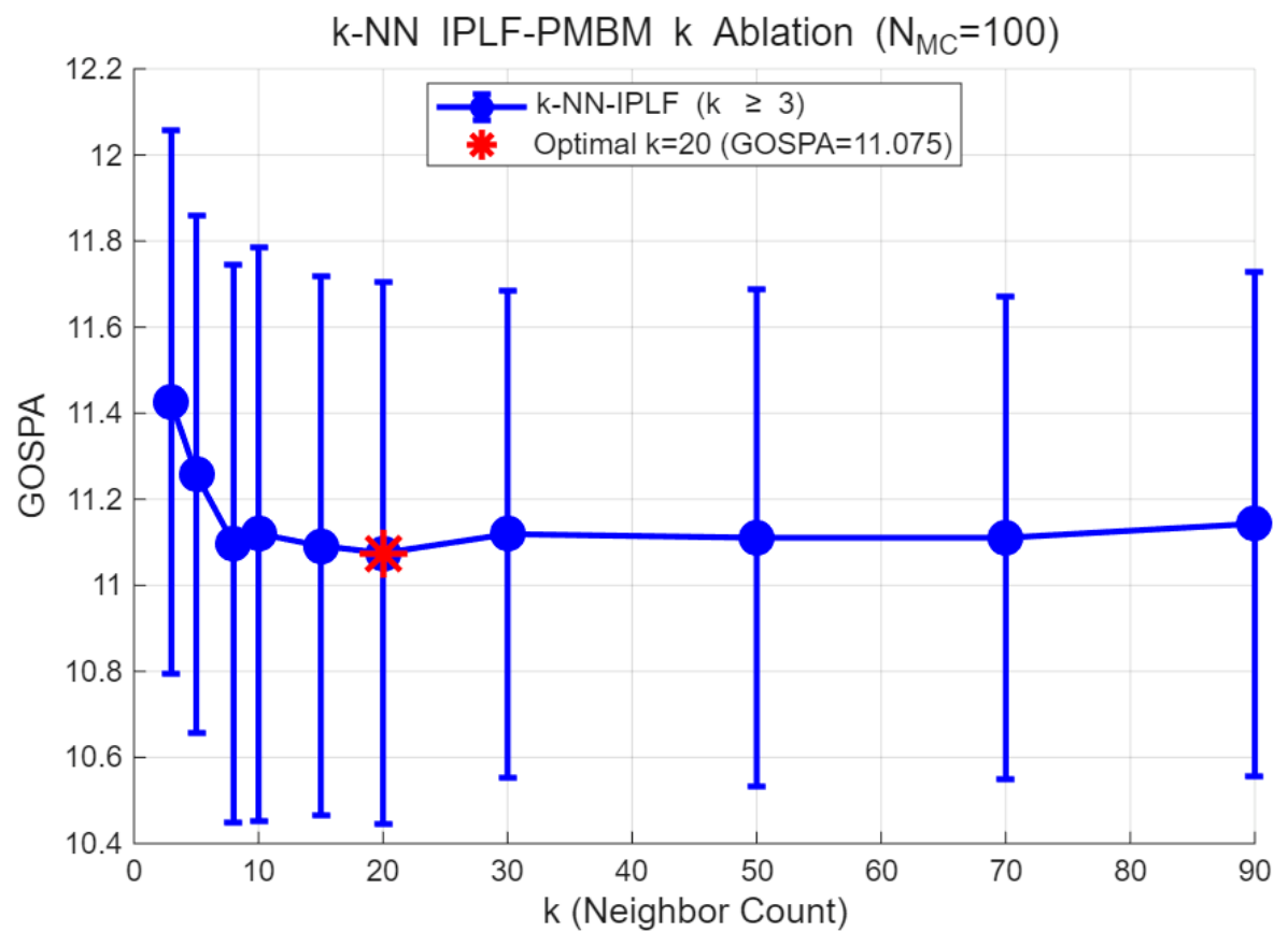
The influence of $k\in \{1,3,5,8,10,15,20,30,50,70,90\}$ on the performance of the k-NN adaptive IPLF–PMBM is tested, with N_MC = 100 runs for each value of k.

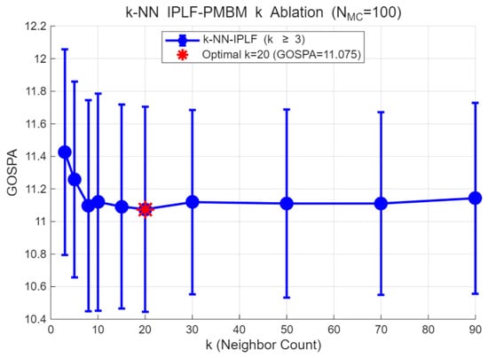
As shown in Figure 7, the GOSPA-k curve exhibits a shallow U-shape, consistent with theoretical expectations. The GOSPA falls from 11.43 at k = 3 to 11.10 at k = 8 and then stays flat out to k = 90. The decreases over the first two steps are 0.17 and 0.16, both significant in paired tests, so a neighborhood holding only a few samples is clearly penalized. Beyond k = 8 the whole curve varies by less than 0.07 and no two settings differ significantly. The minimum is 11.08 at k = 20, the value adopted throughout this paper. The flatness is the shallow optimum anticipated by the bias-variance argument of Section 3.3: once the neighborhood holds a few samples, the estimate is no longer sensitive to the precise sample size.

Figure 7. Ablation experiment results for k.

4.5. Ablation Study on the Update Model

To separate the contribution of the local clutter estimate from that of the IPLF update, the clutter intensity is crossed with the EKF, the UKF, and the IPLF update. The optimal parameters of Section 4.3 and Section 4.4 are adopted, κ₀V = 150 and k = 20, and each of the six configurations is run over NMC = 100 trials with common measurements and random seeds.

As shown in Table 4, the local estimate reduces the average GOSPA from 11.620 to 11.494 under the EKF, from 11.782 to 11.619 under the UKF, and from 11.233 to 11.131 under the IPLF. The three reductions are 0.126, 0.163 and 0.101, and the paired t statistics on the common random numbers are −2.51, −4.03 and −2.69, so the benefit does not depend on the nonlinear update. The IPLF update contributes separately, being 0.388 better than the EKF under the constant and 0.363 better under the local estimate. Since 11.620–0.126–0.363 reproduces the 11.131 of the proposed method, the two effects are nearly additive, and neither is a proxy for the other. The decomposition shows that the gain comes from exchanging missed detections for false alarms: the missed-detection cost of the EKF falls from 93.88 to 64.30 while its false-alarm cost rises from 22.26 to 35.60, the expected behavior of a constant that overestimates the intensity by 3.2 to 9.4 times in the far field.

Table 4. GOSPA of the six configurations over 100 Monte Carlo runs.

Method	Average GOSPA	Std	Localization Cost	Missed- Detection Cost	False-Alarm Cost
EKF-PMBM, fixed κ0	11.620	0.485	30.27	93.88	22.26
k-NN EKF-PMBM	11.494	0.658	46.16	64.30	35.60
UKF-PMBM, fixed κ0	11.782	0.541	29.90	104.54	18.90
k-NN UKF-PMBM	11.619	0.622	42.90	80.56	27.28
IPLF–PMBM	11.233	0.642	42.96	69.10	27.18
k-NN IPLF–PMBM	11.131	0.640	51.19	53.23	33.60

4.6. Uniform Clutter Scenario and Detection Probability

The same comparison is repeated in a scenario where the clutter is spatially uniform, with the expected count of 90 measurements per frame, to check whether the local estimate depends on the non-uniformity. The global constant is set to the true intensity of this field, so the fixed baseline is exact at every range. Two detection probabilities, 0.9 and 0.8, are tested with NMC = 100 runs each and measurements shared by the two methods.

As shown in Table 5, the two methods are indistinguishable in this scenario. At a detection probability of 0.9, the local estimate gives 11.477 against 11.458 for the fixed preset, a difference of +0.019 with t = +0.46 on the paired trials. At 0.8 the values are 12.365 and 12.336, a difference of +0.028 with t = +0.70. Neither difference is significant and both stay below 0.3% of the GOSPA level. This is the expected outcome. When the clutter is uniform the constant is already the true intensity everywhere, so there is no spatial mismatch to remove and the local estimate can only contribute its own estimation noise. That noise is what the 0.02 measures. Lowering the detection probability raises the GOSPA of both methods by about 0.9, with the missed-detection cost rising from 60.66 to 79.23, while their mutual difference stays at 0.02. The conclusion therefore does not depend on the detection rate.

Table 5. GOSPA in the uniform clutter scenario at two detection probabilities.

Pd	Method	Average GOSPA	Std	Localization Cost	Missed- Detection Cost	False-Alarm Cost
0.9	IPLF–PMBM	11.458	0.730	46.70	60.66	37.32
0.9	k-NN IPLF–PMBM	11.477	0.678	47.51	59.70	38.16
0.8	IPLF–PMBM	12.336	0.587	41.48	79.23	44.05
0.8	k-NN IPLF–PMBM	12.365	0.565	40.12	80.13	44.99

4.7. Computational Efficiency Analysis

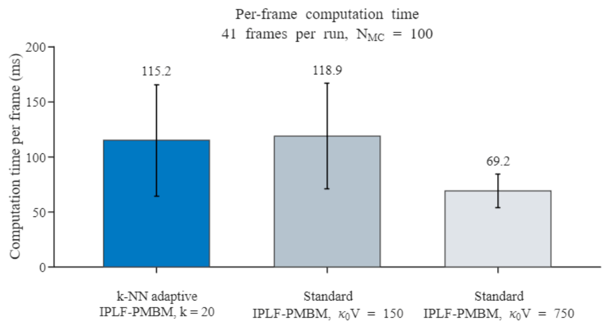
The computational cost is measured in the scenario of Section 4.1, which carries six targets and ninety clutter points per frame on average, so that a frame holds about ninety-three measurements. Each run spans 41 consecutive frames and is repeated over 100 independent measurement realizations for every configuration. The timer is started immediately before the measurement update and stopped immediately after it, so prediction and pruning are excluded from the update figure, and the whole frame is timed separately. All values are per frame and in milliseconds, the neighbor count is k = 20.

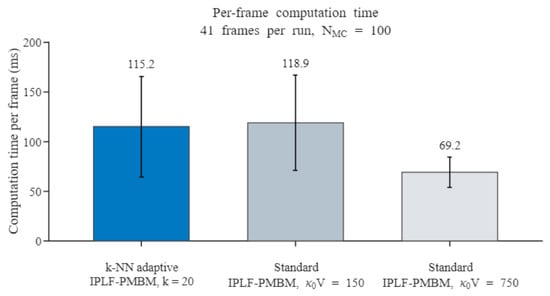
Figure 8 compares the k-NN adaptive filter with the standard filter at the preset of the scenario and at a fivefold preset. The adaptive filter needs 115.2 ms per frame against 118.9 ms at the same preset, a difference of 3.7 ms that lies well inside the run-to-run spread, so the adaptation is not paid for. Suppressing the near-field false alarms leaves fewer global hypotheses to be scored, and this saving covers the cost of the estimate itself. Raising the preset fivefold brings the frame down to 69.2 ms, which shows that the frame cost is governed by the number of hypotheses under test rather than by the clutter model. The spread across runs is large, 50.7 ms for the adaptive filter, because the hypotheses in play change as targets enter and leave. The estimator itself occupies 0.14 ms per frame, which is 0.12% of the frame, and a pointwise implementation of the same formula takes 0.26 ms, so the batch form is 1.84 times faster at the stage it governs. That factor, and not the frame total, is where the implementation claim belongs. At about ninety-three measurements, the distances amount to 8.6 × 10³ evaluations and the sort to 5.7 × 10⁴ comparisons, so the two stages differ only by log₂ m ≈ 6.5 and no change of order is available. The slowest configuration leaves 88% of the one-second refresh interval unused.

Figure 8. Computational cost per frame in the scenario of Section 4.1.

5. Discussion

The error decomposition in Table 2 shows where the adaptation acts. Localization stays between 46.12 and 54.71 across the four filters, so the choice of nonlinear update has little effect on the state estimate of an already confirmed track. The difference is carried by the false-alarm term, which falls from 125.33 for the standard filter and 120.50 for the EKF to 33.60 for the k-NN method. The mechanism is the one set out in Section 4.2. Where clutter crowds the near field, measurements lie close together, the distance to the k-th neighbor is small and the estimated intensity is large, so the newborn existence probability in Equation (6) is driven down and false tracks are blocked; in the far field the reverse holds and genuine targets are born. The adaptation is not free on the missed-detection side. The k-NN error of 53.23 exceeds the 42.10 of the standard filter by about a quarter, for two reasons. The estimate is formed from every measurement in the frame, target echoes included, and the reciprocal of an estimated neighborhood measure is positively biased. The same bias appears in the estimated count, 2.80 for the k-NN method against a true mean of 3.20, while the standard and EKF filters overshoot to 4.86 and 4.40.

Seen from an engineering standpoint, the value of the estimator lies less in the GOSPA margin it holds over a carefully tuned standard filter than in the calibration it removes. The sweep of Section 4.3 shows how strongly the standard filter depends on its preset. Moving κ₀V from 150 down to 10 raises the GOSPA from 11.23 to 26.21 and the false-alarm term from 27.18 to 619.13; moving it up to 400 suppresses births and lifts the missed-detection term to 136.01. In operation the clutter statistics are rarely known in advance and change with range, bathymetry and reverberation, so no single value stays accurate for long. Matching κ₀V to the true expectation of 90 does not reproduce the best fixed value either, since the optimum sits at 150. The adaptive estimate replaces this calibration with one parameter, k, and the ablation of Section 4.4 shows that any value between 8 and 90 gives the same GOSPA to within 0.07.

Several limitations remain. The estimator measures the intensity of the whole measurement process rather than of clutter alone, so its accuracy degrades when target echoes make up a large share of the measurements, and the positive bias noted above produces the missed-detection penalty. The neighborhood measure in Equation (11) assumes that the k-NN ball lies inside the surveillance region; near the sector edges, the ball is clipped, and the estimate is biased. All results come from simulation. Clutter is generated as independent, zone-wise homogeneous Poisson points, whereas real reverberation is spatially correlated, non-Poisson and persistent across scans; the detection probability is constant and multipath, and shadowing is absent; only single-sensor, two-dimensional scenarios with constant-velocity targets are considered. The figures reported here therefore describe the behavior of the algorithm under a controlled, range-dependent profile rather than guarantee performance at sea. Validation with ray-tracing models such as BELLHOP, and ultimately with recorded sonar data, remains necessary. A third limitation concerns the objective itself. The comparison in Section 4.3 shows that the true intensity is not the best setting under GOSPA at this clutter density, which means the metric and the clutter model are not fully aligned; a likelihood-based metric would be a better arbiter and is left for future work.

Future work will follow several lines. Recorded active-sonar data from reverberation-dominated environments will test the method where it matters most. The estimate itself can be sharpened, by correcting its bias or by excluding likely target echoes. The neighbor count can be adapted to the local measurement density instead of being fixed in advance. Multi-static and bistatic configurations, whose clutter statistics vary more strongly in space, form a natural stress test. The estimator transfers to richer filter structures, such as trajectory PMBM, the generalized labeled multi-Bernoulli (GLMB) filter and extended-target PMBM [24]. Finally, target-classification cues such as target strength or acoustic scattering information can be fused into the birth stage to separate genuine targets from clutter more reliably [25].

6. Conclusions

To address the sensitivity of the standard IPLF–PMBM filter to a globally preset clutter intensity in range-dependent underwater clutter, this paper has proposed a local estimator based on the k-nearest-neighbor distance and introduced it into the birth stage of the filter. In a six-target scenario with a power-law clutter profile of ninety points per frame, the method gave a GOSPA of 11.13, which is 22.9% below the standard filter at a preset that underestimates the clutter level and 10.5% and 23.9% below the UKF and EKF counterparts, with the difference carried by the false-alarm term. A sweep over the preset showed that the best fixed value, 11.23, is reached only when the preset is tuned after the fact, at 1.67 times the true mean clutter count, and that the adaptive method matches it without any tuning. The result varies by less than 0.07 over neighbor counts from 8 to 90, and a uniform-clutter control shows that the adaptation neither helps nor harms when the clutter has no spatial structure. The main contributions of this paper are as follows:

(1)

A k-nearest-neighbor estimator of the local clutter intensity has been introduced into the birth stage of the PMBM filter. The estimator follows from a method-of-moments argument, requires no parameter beyond the neighbor count, and is implemented in batch form at a cost of 0.14 ms per frame.

(2)

The estimator has been compared with the standard IPLF–PMBM, UKF-PMBM and EKF-PMBM filters under common realizations. At a preset that underestimates the clutter level, the GOSPA falls from 14.44 to 11.13, and the error decomposition attributes the difference to the false-alarm term. When the standard filter is tuned a posteriori to its best fixed preset, the adaptive method matches it without tuning, 11.13 against 11.23, and its performance is insensitive to the neighbor count over a wide range.

(3)

The pairwise distance matrix is computed once per frame in vectorized form, which brings the local density estimation to 0.14 ms per frame for about ninety measurements. The estimator accounts for 0.1% of the frame time, and the adaptive filter matches the standard filter at the same preset, so the adaptation is obtained at no measurable computational cost.

The k-NN adaptive IPLF–PMBM algorithm therefore offers a solution for underwater sonar multi-target tracking that, in the scenarios considered, requires no manual adjustment of the clutter preset and costs 0.14 ms per frame; validation with more realistic and recorded sonar data is left for future work.

References

- Gong, Y. Research on Multi-Target Tracking Algorithms Based on Probability Hypothesis Density Filter. Ph.D. Dissertation, National University of Defense Technology, Changsha, China, 2021. (In Chinese) [Google Scholar]
- Mahler, R. Multitarget Bayes Filtering via First-Order Multitarget Moments. IEEE Trans. Aerosp. Electron. Syst. 2003, 39, 1152–1178. [Google Scholar] [CrossRef] [Scilit]
- Mahler, R.P.S. Statistical Multisource-Multitarget Information Fusion; Artech House: Norwood, MA, USA, 2007. [Google Scholar]
- Vo, B.-T.; Vo, B.-N.; Cantoni, A. The Cardinality Balanced Multi-Target Multi-Bernoulli Filter and Its Implementations. IEEE Trans. Signal Process. 2009, 57, 409–423. [Google Scholar] [CrossRef] [Scilit]
- Williams, J.L. Marginal Multi-Bernoulli Filters: RFS Derivation of MHT, JIPDA, and Association-Based MeMBer. IEEE Trans. Aerosp. Electron. Syst. 2015, 51, 1664–1687. [Google Scholar] [CrossRef] [Scilit]
- García-Fernández, Á.F.; Williams, J.L.; Granström, K.; Svensson, L. Poisson Multi-Bernoulli Mixture Filter: Direct Derivation and Implementation. IEEE Trans. Aerosp. Electron. Syst. 2018, 54, 1883–1901. [Google Scholar] [CrossRef] [Scilit]
- Xie, J.C. Research on PMBM-Based Multi-Extended Target Tracking Algorithms. Ph.D. Dissertation, Xidian University, Xi’an, China, 2022. (In Chinese) [Google Scholar]
- Miao, T.; El Amam, E.; Slaets, P.; Pissoort, D. Multi-Target Tracking and Detection, Fusing RADAR and AIS Signals Using Poisson Multi-Bernoulli Mixture Tracking, in Support of Autonomous Sailing. In Proceedings of the International Naval Engineering Conference and Exhibition (INEC 2020), Online, 5 October–9 November 2020; pp. 1–13. [Google Scholar]
- Lee, H.; Choi, J.; Heo, S.; Huh, K. Centralized Multi-Sensor Poisson Multi-Bernoulli Mixture Tracker for Autonomous Driving. IFAC-PapersOnLine 2022, 55, 40–45. [Google Scholar] [CrossRef] [Scilit]
- Narykov, A.; Wright, M.; García-Fernández, Á.F.; Maskell, S.; Ralph, J.F. Poisson Multi-Bernoulli Mixture Filtering with an Active Sonar Using BELLHOP Simulation. In Proceedings of the 25th International Conference on Information Fusion (FUSION), Linköping, Sweden, 4–7 July 2022; pp. 1–7. [Google Scholar] [CrossRef] [Scilit]
- Zhu, J.; Xie, W.; Liu, Z. Student’s t-Based Robust Poisson Multi-Bernoulli Mixture Filter under Heavy-Tailed Process and Measurement Noises. Remote Sens. 2023, 15, 4232. [Google Scholar] [CrossRef] [Scilit]
- Zhang, Y.; Li, Y.; Li, S.; Zeng, J.; Wang, Y.; Yan, S. Multi-Target Tracking in Underwater Multistatic AUV Networks with a Robust Poisson Multi-Bernoulli Filter. Ocean Eng. 2023, 284, 115167. [Google Scholar] [CrossRef] [Scilit]
- Deleskog, V.; Jonsson, O.; Nygårds, J.; Hendeby, G. Poisson Multi-Bernoulli Mixture Filtering with Multistatic Passive Bistatic Radar. In Proceedings of the 27th International Conference on Information Fusion (FUSION), Venice, Italy, 8–11 July 2024; pp. 1–8. [Google Scholar] [CrossRef] [Scilit]
- Julier, S.; Uhlmann, J.; Durrant-Whyte, H.F. A New Method for the Nonlinear Transformation of Means and Covariances in Filters and Estimators. IEEE Trans. Autom. Control 2000, 45, 477–482. [Google Scholar] [CrossRef] [Scilit]
- Wan, E.A.; Van Der Merwe, R. The Unscented Kalman Filter for Nonlinear Estimation. In Proceedings of the IEEE 2000 Adaptive Systems for Signal Processing, Communications, and Control Symposium (AS-SPCC), Lake Louise, AB, Canada, 1–4 October 2000; pp. 153–158. [Google Scholar] [CrossRef] [Scilit]
- García-Fernández, Á.F.; Svensson, L.; Morelande, M.R.; Särkkä, S. Posterior Linearization Filter: Principles and Implementation Using Sigma Points. IEEE Trans. Signal Process. 2015, 63, 5561–5573. [Google Scholar] [CrossRef] [Scilit]
- García-Fernández, Á.F.; Ralph, J.; Horridge, P.; Maskell, S. Gaussian Trajectory PMBM Filter with Nonlinear Measurements Based on Posterior Linearization. In Proceedings of the 25th International Conference on Information Fusion (FUSION), Linköping, Sweden, 4–7 July 2022; pp. 1–8. [Google Scholar] [CrossRef] [Scilit]
- Silverman, B.W. Density Estimation for Statistics and Data Analysis; Chapman and Hall: London, UK, 1986. [Google Scholar]
- Park, S.H.; Chong, S.Y.; Kim, H.J.; Song, T.L. Adaptive Estimation of Spatial Clutter Measurement Density Using Clutter Measurement Probability for Enhanced Multi-Target Tracking. Sensors 2020, 20, 114. [Google Scholar] [CrossRef] [Scilit] [PubMed]
- Chen, X.; Tharmarasa, R.; Kirubarajan, T.; Pelletier, M. Integrated Clutter Estimation and Target Tracking Using Poisson Point Processes. IEEE Trans. Aerosp. Electron. Syst. 2012, 48, 1210–1235. [Google Scholar] [CrossRef] [Scilit]
- Loftsgaarden, D.O.; Quesenberry, C.P. A Nonparametric Estimate of a Multivariate Density Function. Ann. Math. Stat. 1965, 36, 1049–1051. [Google Scholar] [CrossRef] [Scilit]
- Bar-Shalom, Y.; Li, X.R.; Kirubarajan, T. Estimation with Applications to Tracking and Navigation: Theory, Algorithms, and Software; Wiley: New York, NY, USA, 2001. [Google Scholar]
- Rahmathullah, A.S.; García-Fernández, Á.F.; Svensson, L. Generalized Optimal Sub-Pattern Assignment Metric. In Proceedings of the 20th International Conference on Information Fusion (FUSION), Xi’an, China, 10–13 July 2017; pp. 1–8. [Google Scholar] [CrossRef] [Scilit]
- Li, P.; Chen, C.; Sun, Y.; Wang, W. Poisson Multi-Bernoulli Mixture Filter for Multiple Extended Object Tracking Using Kolmogorov–Smirnov Test. IEEE Sens. J. 2025, 25, 6541–6555. [Google Scholar] [CrossRef] [Scilit]
- Bai, M.; Zhang, Q.; Yu, R.; Zhang, Y.; Sun, B. RCS Information Aided Poisson Multi-Bernoulli Mixture Filter in Clutter Background. IEEE Sens. J. 2024, 24, 5039–5052. [Google Scholar] [CrossRef] [Scilit]
Disclaimer/Publisher’s Note: The statements, opinions and data contained in all publications are solely those of the individual author(s) and contributor(s) and not of MDPI and/or the editor(s). MDPI and/or the editor(s) disclaim responsibility for any injury to people or property resulting from any ideas, methods, instructions or products referred to in the content. |
© 2026 by the authors. Licensee MDPI, Basel, Switzerland. This article is an open access article distributed under the terms and conditions of the Creative Commons Attribution (CC BY) license.