Scaling of Submerged Rubble-Mound Models

Abstract

Submerged mound breakwaters are viable eco-friendly structures for shore protection, serving as an alternative to their emerged counterparts. Physical modelling is still extensively used to study coastal processes and provide calibration and verification data. The aim of this study is to present a methodology adapted exclusively to submerged structures to tackle the problem of scale effects when determining the size of the core material. Such effects have been adequately studied in emerging mounds, thus forming the rationale for the present work. Hydrodynamic pore pressures inside the underwater body were evaluated using experimental results; these were then input into the extended Forchheimer equation, including the nonlinear effects of velocity upon the drag force induced by the pressure gradient. The experimental results used were satisfactorily compared with other laboratory measurements and with results from two numerical models. The proposed calculation methodology combined with the corresponding hydraulic resistance can yield a correction factor K for model downscaling of the breakwater material. Numerical applications are given along with design nomographs providing the K value. The presented results on the required scale correction to be applied to determine the sizing of the core material in physical models of submerged mound breakwaters deviate significantly from those related to emerging breakwaters, thus justifying the undertaking of the present work.

1. Introduction and Scope

Development of the coastal zone is increasing globally, intensified by growing climate-driven threats. The heavy stress on the ecosystems supported by this zone necessitates the adoption of a management strategy that aims to address relevant environmental issues while also protecting human coastal settlements and activities. Oftentimes, a compromise is reached whereby the coastal environment is duly respected in balance with local communities’ needs. In this context, coastal structures, intended to control coastline erosion, are introduced to serve this aforementioned dual function.

The realm of nature-based solutions for coastal zone management includes a range of “soft” interventions, e.g., control of natural dunes, development of mangrove forests, restoration of salt marshes, and enhancement of coral reefs or seagrass meadows (see, e.g., [1]). However, the large scale that these solutions require to provide an efficient level of coastal resilience leaves room for the introduction of smaller-scale systems that can be derived from an array of conventional coastal structures with eco-friendly modifications. A specific class of this type of structure is the submerged breakwater, also sometimes referred to as the “reef breakwater”.

Submerged mound breakwaters result from a shape modification of the emerged rubble mound and can become, under certain constraints, a shore protection structure that serves as an alternative to its emerged counterpart. The main process of wave energy dissipation is through induced wave breaking. This submerged structure displays several environmental advantages; for example, it allows for increased water renewal to its lee, provides improved aesthetic value for the landscape, occupies a smaller seabed area, especially when narrow-crested, and requires less material compared to traditional breakwaters. Additionally, submerged breakwaters can be constructed from homogeneous (or two-layered) material, especially in less severe wave environments, providing support to local marine life through their more porous structure. However, all of the previously mentioned benefits are offered at a cost: submerged breakwaters cannot deflect a large percentage of wave energy attacking the shore; hence, they are only practically applicable along coasts with up to medium wave energy exposure located in micro-tidal environments where appropriate freeboards can be maintained.

Despite recent notable progress in numerical modelling to address coastal hydrodynamic problems, physical models are still broadly used to study physical processes and provide calibration and verification data, thus providing a strong tool for relevant research and practical applications. Physical models are typically preferable to field measurements and observations. Indeed, although the latter provide the best information [2], they are usually costly, while the obtained data are difficult to interpret due to the large range of natural variables involved in the measurements.

In order to be able to correctly render results from physical model tests, caution should be exercised when scaling down the models. In general, the requirement is that the behaviour of a laboratory model should be representative of its prototype in all aspects. Proper scaling is achieved when the major parameters affecting hydrodynamic sea–structure interactions can be maintained between the prototype and model, as determined through the application of similitude criteria proportionally significant to the process under study. The quantification of scale effects measures the deviation of the hydraulic behaviour between a physical model and its prototype.

The main cause of adverse scale effects in models built to study hydrodynamic processes in and around rubble-mound breakwaters links directly with flow conditions inside the mound. In fact, prototype flow conditions should be maintained throughout the body of a rubble-mound structure model under wave action [3]. This requirement may not be met under certain layouts where the size of stone units is quite small, thus inducing viscous (upscaled) forces that are greater in the model than in the prototype. This drawback results in a dissimilar reproduction of the hydrodynamic field around the structure, giving rise to improper estimates of variables such as wave transmission factors.

The above issue has been discussed quite extensively in the context of practical applications of emerged rubble-mound breakwaters, as will be seen in the following section. However, although substantial work has been conducted on a range of topics related to submerged breakwaters, e.g., wave transmission and structural resistance, the corresponding problem of scale effects has not yet been addressed for these structures to our knowledge, which is critical as their application continues to gain momentum. Therefore, the only solution for researchers and designers alike is to apply the results for the emerged mounds, irrespective of the type of breakwater under examination. However, a simple comparison of the wave modification when it attacks either an emerged or a submerged obstacle leaves no doubt that the two associated hydrodynamic fields are significantly different. This gives full justification, we believe, for further research on the topic of scale effects in submerged rubble-mound breakwaters.

The scope of this work is to present a method for deriving a practical core stone-size correction tailored exclusively to submerged rubble-mound breakwaters, supported by relevant application recommendations. The requirement that prompted this study relates to estimating the wave transmission coefficient behind submerged breakwaters, but clearly there is no restriction on the results to this topic alone. Associated results enable comparison with the current practice mentioned above, thereby justifying the use of the method introduced in this paper.

The proposed method for deriving a modified scale factor is presented in Section 3, while Section 4 is devoted to the Darcy–Forchheimer equation and some specific advances upon it. Original work on the pore pressure gradient inside the submerged breakwater body is included in Section 5, and an application example is presented in Section 6. Finally, a discussion of the results and related facets of the research is presented in Section 7, followed by the conclusions in Section 8.

2. Background Knowledge

As noted in the previous section, there are no published studies or technical recommendations addressing scale effects in submerged breakwater models. The closest topic concerns scale effects in the emerged counterparts of the submerged structures studied in this paper. For these emerged structures, several works can be cited that address methods for sizing the model stone material, especially of the finer grade, to avoid spurious scale effects on hydrodynamic parameters such as wave transmission. The method proposed in [4] was based on analytical considerations and available data, from which a design nomograph was developed and redrawn in the classical work [3]. In [4], it was suggested that a scale correction factor K > 1.0 may be needed for the downscaling of model core stones, depending on the actual configuration, including wave climate parameters. It was also assumed in [4] that scale effects are negligible in the outer armour layers of an emerged rubble-mound breakwater, as relatively large rocks are usually modelled in these layers. In [5], a method was proposed based on semi-empirical equations for sizing stone diameter in rubble-mound structures. The study was based on experiments with a typical model porosity of n = 0.46. In 1979, [6] extended Keulegan’s method [5] to account for porosity as a variable by introducing a Reynolds number Re involving n. It was found that, under Froude scaling, turbulent dissipation dominates energy losses. Thus, for prototypes with Re > 2000, size correction is needed only when the corresponding model Re falls below that threshold.

Following the above initial research period, it became apparent that a deeper understanding of wave kinematics inside porous bodies was needed to gain a more comprehensive understanding of scale effects. In this context, the decay and damping rate of standing waves was studied [7] on various horizontal porous seabeds consisting of relatively small gravel (median nominal diameter D_n50 ranging from 0.72 cm to 3.47 cm). The results illustrated that, for small gravel, the energy lost through fluid motion is affected not only by inertia and turbulence in an oscillating flow but also by the presence of laminar flow characteristics, adding further to energy loss. This issue was also addressed in [8], where it was noted that, in general, flow through a downscaled permeable structure may be accompanied by scale effects under certain conditions. In particular, in small models, the flow may be laminar, while under prototype conditions, the corresponding flow can be turbulent in a certain area of the structure. In the same study [8], the relative importance of inertial, turbulent, and laminar resistance components in analytical formulations was investigated in relation to the stone size of a porous medium. It was estimated therein that, for stone material with D_n50 ranging up to 6.1 cm under a 1:10 scale, a nonlinear unsteady porous flow model should incorporate all three components. In a 1995 publication [9], the kinematics and dynamics of oscillatory flow were studied experimentally in an idealized porous structure, in both emerged and submerged configurations.

Further to the notable treatise on laboratory techniques [3], a DELOS project report [10] deals with the theoretical problem of scale effects in models of rubble-mound breakwaters under wave action. As noted previously, neither of these works deals explicitly with submerged rubble mounds.

It will be seen in the following sections that knowledge of pore pressures inside the body of breakwater mounds is critical for evaluating the hydraulic resistance required to apply the extended Forchheimer equation, an enhanced variation of the original Darcy–Forchheimer equation. This former equation is used as a basic tool to address the problem under consideration, leading finally to the evaluation of any scale effect present in the case examined. A substantial body of literature has been published over time, based mainly on laboratory and field measurements, regarding the prediction of pore pressures inside emerged rubble-mound breakwaters (see, e.g., [11,12,13,14,15,16,17]). The results of those studies have contributed to a better understanding of the flow regime and the associated attenuation of hydrodynamic pore pressures in the core of emerged rubble mounds.

Measurements inside a rubble-mound core were taken [18] to study wave transmission through a low-crested structure. That research was part of the aforementioned European research project, which also included pore pressure measurements above the flume bed. With the aim of demonstrating the validity of the VoF-type model COBRAS beyond small-scale model setups, simulations of a laboratory experiment involving a submerged, multilayered rubble-mound breakwater at near-prototype scale were presented using the said numerical model. Some of those results will be used in Section 5 to compare corresponding data from experimental research used in this investigation. Pore pressures inside submerged breakwaters subjected to travelling waves were systematically measured in physical model experiments, as presented in [19]; the results were used herein to formulate the hydraulic resistance inside the mound. In addition, data on hydrodynamic pressures in submerged rubble mounds were obtained from laboratory experiments at TUDelft [20]; these were also used for comparison with the main data set noted previously.

The Darcy–Forchheimer equation has been developed over time since its initial formulation from the original Darcy equation. It is a semi-empirical expression that can be used either in conjunction with wave propagation numerical models or independently to calculate hydraulic resistance inside structures interacting with surface waves. In the following, it will be used in its latter capacity. The main challenge in using this equation is the determination of the factors involved in its hydraulic resistance components (see Section 4). In this context, permeability measurements were carried out [21] in a channel filled with coarse granular material under stationary or oscillatory flow. A model was proposed that was considered suitable also for submerged breakwaters under wave action. However, in that work, the porous models were confined within a U-tube channel, and the resulting turbulence should be considered representative of smaller models rather than a typical physical model of a submerged mound. For a review of the evolution of the resistance terms in the Darcy–Forchheimer equation, see also [22,23], among many others.

3. Proposed Methodology

Traditionally, the hydrodynamic response of rubble-mound structures is studied using physical models downscaled according to the Froude scaling law, which neglects viscous effects. This introduces differences in the flow regime between the prototype and the model, because the inherent scaling of the stone material creates laminar flow in regions that may be dominated by turbulent flow in the prototype. These differences impair the accurate reproduction of the flow field under certain conditions, thereby limiting the reliability of physical modelling. The present study focuses on providing the required correction to the geometric similarity of the fine particle size to account for this discrepancy when needed.

The methodology used in this paper was developed to allow for easy application in designing experiments with physical models. It is based on knowledge of two parameters: the pore pressures in the mound body under wave attack and the so-called hydraulic resistance over the same area. These two parameters are interrelated through a suitable version of the Darcy–Forchheimer equation, and eventual inconsistencies between the two map the scale effect. Such a framework is also observed in research associated with emerged breakwaters (see, e.g., [24]).

Since the scope of this work is to provide support for practical applications, it is necessary to employ sensible approximations when treating the theoretical relations. One such example concerns the estimation of the dynamic component p of the pore pressure inside the rubble mound. Its partial derivative with respect to space is critical to solving the extended Forchheimer equation, which yields the required particle size. As waves pass through the breakwater, one can easily imagine that the value of p at any given moment varies across the structural cross-section, leading to equally variable results. However, only one result is needed in practice for sizing the core material of the mound. This challenge is addressed by adopting carefully selected approximations, as will be seen in Section 5.

Another simplification relates to the loose interplay allowed between D and D_n50, where D denotes the mean diameter of nearly homogeneous stones. As mentioned in Section 1, homogeneous submerged breakwaters, which constitute a subtype of submerged mounds, maintain significant environmental value due to the support they can provide to marine ecosystems.

The methodology used in this paper can be divided into the following successive steps:

(a)

Starting from the data of the prototype we wish to model, the coefficients of the extended Forchheimer equation are calculated. This allows the hydraulic resistance part of that equation to be expressed in terms of a characteristic (horizontal) velocity in the porous core area of the structure.

(b)

We define a representative value of the pressure gradient from experimental results that corresponds to the hydraulic resistance applicable across the structure’s cross-section. The relations proposed for this purpose apply equally to both prototype and model.

(c)

We apply the extended Forchheimer equation to the prototype structure and obtain the relevant characteristic velocity value inside the core.

(d)

The resulting velocities from (c), downscaled to the model size, are combined with the pressure gradient from (b) to provide, through the aforementioned equation, a nominal size of the model core material in terms of, say, the median nominal diameter D_n50.

(e)

The ratio of the resulting sizes for the prototype (a) and model (d) will give the required geometrical scale to be applied to the core material, so that the physical model can credibly reproduce the prototype hydrodynamic field. In general, the scale found may differ from the overall linear scale applied in the model design, especially in cases of fine core material.

These steps will be further elaborated upon in the sections to follow.

4. The Extended Forchheimer Equation

At the dawn of the 20th century, the classical Darcy equation, describing the velocity field in a streaming flow due to a pressure gradient inside a porous medium, was extended by Forchheimer to include the nonlinear effects of velocity on the drag force induced by the said gradient. Later, the need to describe the same problem under unsteady conditions, such as those associated with propagating surface waves, led to the so-called extended Forchheimer equation, which includes an extra term describing the inertial contribution to the total force. This latter version of the Darcy–Forchheimer equation reads [25]

$$I=au+bu\left|u\right|+c{\displaystyle \frac{\partial u}{\partial t}},$$

(1)

where I is the pressure gradient, u is the discharge (or filter) velocity related to the total cross-section of the medium across the flow, t is the time, and a, b, and c are empirical coefficients linked to the porous flow conditions. The pressure (or hydraulic) gradient is expressed by

$${\rm I}={\displaystyle \frac{-1}{\rho g}}{\displaystyle \frac{\partial p}{\partial x}}$$

(2)

where ρ is the water density, g is the acceleration due to gravity, x is a horizontal dimension.

The characteristic velocity u is expressed by u = nu_i, where n is the porosity and u_i is the seepage (or pore) velocity, i.e., the averaged velocity over a uniformly distributed pore space. It is recommended to take the maximum discharge velocity as representative of the flow. The first term in the right-hand side of Equation (1) refers to the linear viscous contribution to the total drag (Darcy-type flow), the second refers to the nonlinear turbulent drag component, and the third refers to the inertial contribution to the total frictional forces.

Coefficients a, b, and c in Equation (1) depend on the stone size and flow conditions. Therefore, they are not constant under oscillatory flow conditions. However, in engineering practice, these coefficients are assumed to be constant for any specific configuration of the problem, including the Keulegan–Carpenter (KC) number defined below [22]. This number uses the maximum seepage velocity as the representative velocity, leading to the condition that u takes its maximum value in Equation (1). Under this condition, c becomes zero at the peak velocity u and can therefore be neglected; in any case, the period during which this term can be significant is quite short (see [21]). Regarding a possible resistance component associated with the convective u component, it can be argued that such an effect would be quadratic in u and, therefore, would be incorporated and “captured” in the term b in the equation (see [26]). Van Gent’s expressions for the a and b coefficients are given in Equations (3) and (4), respectively:

$$a={\alpha }_p{\displaystyle \frac{{\left(1-n\right)}^2}{n^3}}{\displaystyle \frac{\nu }{g{D}_{n50}^2}}$$

(3)

where α_p is a parameter to be given below (Equation (6)) and

$$b={\beta }_p\left(1+{\displaystyle \frac{7.5}{KC}}\right){\displaystyle \frac{1-n}{n^3}}{\displaystyle \frac{1}{g{D}_{n50}}},$$

(4)

with KC being the Keulegan–Carpenter number

$$KC={\displaystyle \frac{u{T}_m}{n{D}_{n50}}},$$

(5)

where T_m is the mean period of the oscillatory flow and β_p is defined in the following by Equation (7).

α_p and β_p are parameters usually expressed in terms of constants; values for α_p range roughly between 200 and 2000, while those for β_p range within 0.5–1.5 (see [23]). Constant values for the resistance coefficients for a broad range of flow conditions were also recommended based on calibrations presented in [27]. Alternatively, relationships have been proposed between the above parameters and specific data for the porous medium [28]. However, application of those relations to several cases did not show the expected behaviour, e.g., for increasing D_n50, these expressions did not yield decreasing scale correction. Therefore, in this work, van Gent’s proposal was adopted instead as follows:

α_p = α = 1000

(6)

β_p = β = 1.1

(7)

Please note that α_p and β_p are nondimensional, while the same happens with the terms in Equation (1). Since the final scale correction K values depend on both α_p and β_p, a simple sensitivity analysis was undertaken to estimate that dependence. Representative results are given below. In Table 1, an example of sensitivity analysis is given for a wave of T 6.0 s and H_i 1.5 m with respect to a varying a_ρ coefficient for a scale of 1:10, a prototype core D_n50 = 0.20 m, and a horizontal distance ΔL = 5.0 m, with b_ρ being constant. In Table 2, associated results are given for the same wave and geometrical characteristics, i.e., with a varying b_ρ coefficient and a_ρ being constant. It appears that K values vary with varying coefficients but not significantly for practical applications, provided the coefficient values fall within an acceptable range, say 15%, around the assumed values given in Equations (6) and (7). It is also noted that K increases with increasing α_p, as shown in Table 1, while the opposite holds with increasing β_p.

Table 1. Sensitivity analysis given for a wave of T = 6.0 s and H_i = 1.5 m with respect to a_ρ for a scale of 1:10, with b_ρ = 1.1 and prototype core D_n50 = 0.20 m, ΔL = 5.0 m, and n = 0.4.

K	aρ	bρ
1.25	500	1.1
1.3	750
1.35	1000
1.38	1250
1.45	1500

Table 2. Sensitivity analysis given for a wave of T = 6.0 s and H_i = 1.5 m with respect to b_ρ for a scale 1:10, with a_ρ = 1000 and prototype core D_n50 = 0.20 m, ΔL = 5.0 m, and n = 0.4.

K	bρ	aρ
1.4	0.7	1000
1.35	0.9
1.34	1.1
1.32	1.3
1.3	1.5

The model prescribed by Equation (1) was further updated as suggested in [29]; a new term was included, varying like ~u^3/2 to smoothly cover the step between laminar (a-term) and turbulent (b-term) ranges. That extra term is described by Cu|u|^1/2, with C given by the following relation:

$$C=4.5{\displaystyle \frac{1-n}{n^3}}{\displaystyle \frac{{\nu }^{1/2}}{g{D}_{n50}^{3/2}}}$$

(8)

where ν denotes the kinematic viscosity of seawater, taken in the applications as 10⁻⁶ m²/s.

It is noted that this extra term is again non-dimensional and that the absolute value is misplaced in several publications.

The combination of Equations (1) and (2) gives:

$${\displaystyle \frac{-1}{\rho g}}{\displaystyle \frac{\partial p}{\partial x}}=au+bu\left|u\right|+c{\displaystyle \frac{\partial u}{\partial t}}$$

(9)

As can be easily verified, each term in Equation (9) is nondimensional since p/ρg is expressed in length units (height of water column). Evaluation of the left-hand term is performed in the following section.

5. Pore Pressure Gradient

The originality of this paper lies in examining a different hydrodynamic configuration from those previously studied to estimate the scale effect on the stone size of physical models of mound breakwaters. Indeed, previous research has focused on evaluating this effect for emerged breakwaters subjected to sea waves. However, as stresses on the coastal environment increase, the submerged counterpart of the conventional rubble-mound structure is gaining importance in microtidal waters as a quasi-hard coastal protection option. Obviously, the hydrodynamic field around a submerged mound is fundamentally different from that associated with emerged structures, simply because, in the former case, waves can travel to the lee side of the breakwater, whereas this is not the case in the conventional configuration. This major difference in wave–structure interaction directly affects the pore pressure distribution inside the porous obstacle. An estimate of these pressures, suitable for physical model design, is presented below.

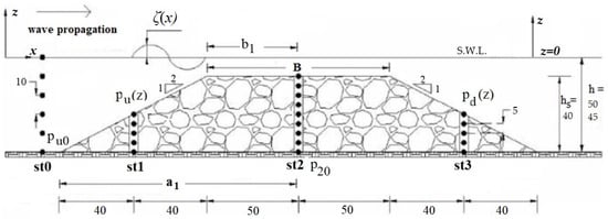
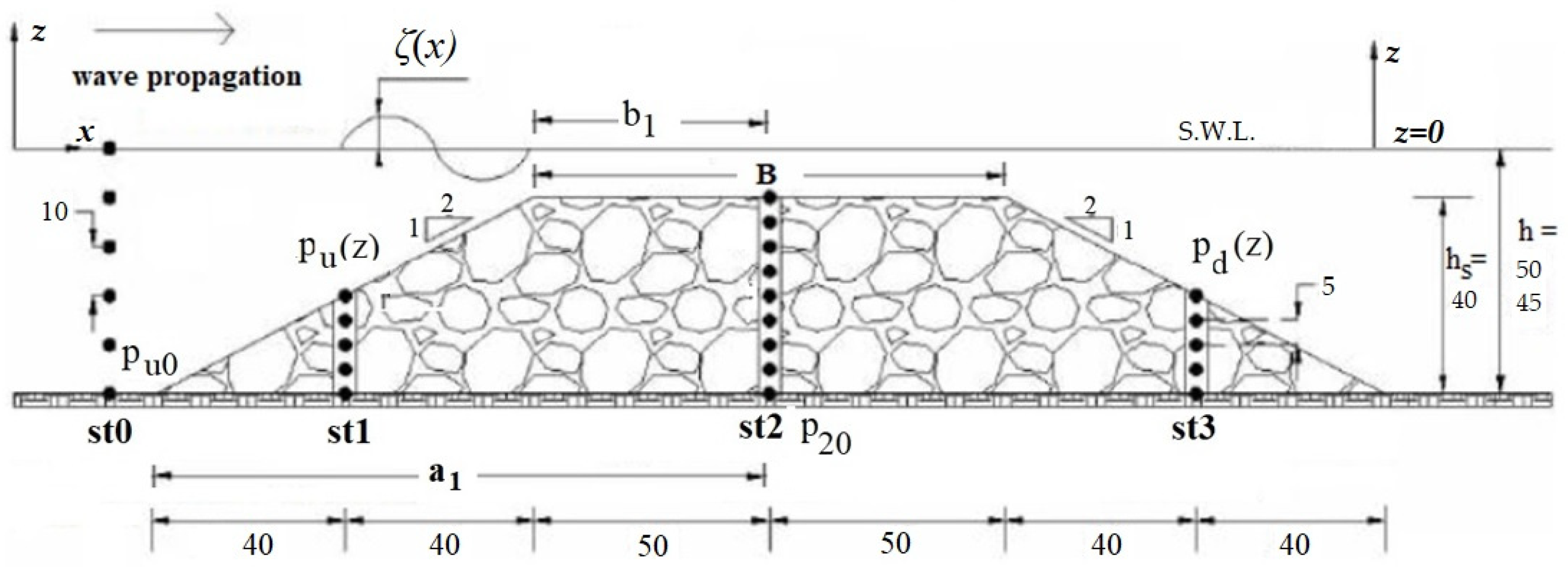
For the purpose of determining the pressure field inside the breakwater body, relevant experimental results were used [19]. Measurements of hydrodynamic pressures were conducted in a flume at the NTUA port structures laboratory for breaking and non-breaking regular waves. The experimental setup is shown in Figure 1, where the dots indicate the measurement points. Pressure data were also taken at a reference station (st0) upstream of the mound.

Figure 1. Model cross-section with measurement points (•) for two water depths (lengths in cm).

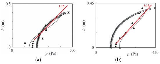
The model structure was made of uniform natural stones with D_n50 = 0.08 m, with slopes of 1:2 on both sides. Their size distribution was rather peaked, giving a high porosity of n = 0.52. Regular waves were used as the input, and a range of cases was tested, covering various combinations of wave height, wave period, and water depth. For the purpose of the present study, results from two cases were used to cover both breaking and non-breaking waves. These experimental results were used in [19] to verify a Boussinesq-type numerical model coupled with an extended Forchheimer equation developed following [30]. Comparison of that model with COBRAS, a RANS-equations model employing volume averaging inside the porous structure, showed performance at least as good as that of the RANS model, as shown in Figure 2, where results from the latter model are denoted by (*). Therefore, for the present study, it was decided to use the results of the Boussinesq-type model in conjunction with the mentioned experimental measurements.

Figure 2. Vertical pressure gradient along the middle of the structure for nonbreaking (a) and breaking (b) waves: (▲) measurements, (-) Boussinesq-type model, (ж) COBRAS used in this application, (•) presence of boundary layers on the seabed.

Comparisons were also made with experimental results obtained at TUDelft using irregular waves [20]. It was found that, for an incident wave height H_i = H_m0, the mean pressures are somewhat higher under regular waves, which is expected due to the increased energy carried by these waves under these conditions. Typically, in regular-wave experiments, the incident wave height H_i is defined at the structure’s offshore toe, where wave–structure interaction generates additional components that affect wave regularity. Therefore, its calculation generally follows the same approach as that used when irregular waves are generated, with H_i represented by the significant wave height, as adopted in this article. Nevertheless, the above disagreement still applies, especially in shallow water, due to the substantial differences between the underlying spectra. In special cases where this disagreement is significant, a simple correction can be applied based on fundamental hydrodynamics. However, regarding pressure gradients, the results were sufficiently close for both regular and irregular waves (see also Figure 5 in [14]). It should be noted that the use of regular rather than random waves in experimental work of this kind is recommended, since the maximum values of hydrodynamic pressures of interest are more reliable under regular waves than under random waves, where they can cover extended ranges.

The principal direction of the pressure gradient should coincide with that of the main flow, i.e., along the horizontal cross-section, as is the case for u. Therefore, we need to focus on evaluating the dynamic component of the pressure induced by the propagation of the wave pulse along x. The experimental and numerical results obtained at station #2 (st2) were first used to determine the variation in p along that vertical. The simple relation proposed for the purposes of this investigation reads

$${\displaystyle \frac{1}{\rho g}}{\displaystyle \frac{\delta p}{\delta z}}={\displaystyle \frac{1}{15}},$$

(10)

where δ denotes the value difference.

The above relation is based on laboratory measurements and numerical results from the previously mentioned Boussinesq-type model and a VARANS model (COBRAS), presented in Figure 2. As can be seen in that figure, Equation (10), denoted in red, provides a reasonably close approximation to the actual nonlinear pressure distribution, suitable for the purposes of the present study. The dotted portion of the proposed line refers to the presence of boundary layers on the seabed, where pressures cannot be credibly predicted or required for this application. It is also encouraging that the same rate of pressure change along the vertical is obtained for both breaking and non-breaking waves.

The other relations needed to define a mean pressure gradient inside the structure were obtained in a similar manner, based on the above experimental and numerical model results as well as on existing knowledge for emerging breakwaters. These are presented in the following in a condensed way. Firstly, a connection is needed between p₂₀ (2 for st2, 0 for point on the seabed, see Figure 1) and the corresponding pressure p_u0 at the slope toe. Following [14], this can be expressed by

$$p_{20}=exp\left(-\epsilon k^{\prime }{a}_1\right)p_{u0}$$

(11)

where $\epsilon ={\displaystyle \frac{a_{\epsilon }\sqrt{n}{L}_p^2}{H_{m0}\Delta L}}$ and $k^{\prime }={\displaystyle \frac{2\pi }{{L_p}^{\prime }}}={\displaystyle \frac{7.434}{L_p}}$ and H_m0 is the spectrum-based wave height, L_p’ is the peak wavelength inside the body of the structure, Lp is the peak wavelength at the structure toe, a₁ is half of the base length, and α_ε = 0.015.

As noted in Section 5, the H_i for regular and H_m0 for irregular waves can in most cases be interchanged; under specific hydrodynamic conditions, the relevant theoretical wave height correction can easily be imposed. The wave number given above is modified to cope with the wavelength transformation in the porous material: a simple expression is used for the internal wavenumber k’, with ${L_p}^{\prime }$ = Lp/(1.4)^1/2, as proposed in [31]. Pressure p_u0 can be derived from the general expression of reference pressure p_u(z) given in Equation (12), which estimates the hydrodynamic pressure over the offshore slope of the breakwater. The background of this relation comes from analysis of laboratory results in TUDelft [20] that showed the expression ((p_u(z)/ρgH_m0)·(h/H_m0)·(h/ΔL)^1/2 to be practically constant; hence it appears that

$${\displaystyle \frac{p_u\left(z\right)}{\rho g{H}_{m0}}}=2{\displaystyle \frac{H_{m0}}{h}}{\left({\displaystyle \frac{\Delta L}{h}}\right)}^{1/2}cosh\left[k\left(h+z\right)\right],$$

(12)

where k is the wavenumber in free space and ΔL is a characteristic horizontal dimension of the porous structure. Typically, ΔL can be taken, in this problem, as a characteristic length of half the horizontal dimension of the trapezoidal breakwater at mid-height. This definition was considered appropriate because the pressure gradient decreases monotonically only up to the axis of the submerged structure. The above relation shows a considerable increase in pressures on the offshore slope compared with those in the free field. This increase is due to the very presence of the underwater obstacle, and for a porous medium, it is related to a characteristic length of the latter along the horizontal on the cross-section.

Regarding the pressure p_d(z) on the inshore face of the structure, the following simple relation was arrived at:

$$p_d\left(z\right)=0.95p_u\left(z\right)$$

(13)

The factor 0.95 in this relation results from a simple evaluation of the pressure ratio at corresponding points on the offshore and inshore slopes, which is sufficient for practical applications. In fact, the means of the measured and numerically predicted pressure ratios at the uppermost points of Section 1 and Section 3 were calculated (see Figure 1 and [19]). Excluding one outlier measurement, these ratios ranged between 0.84 and 1.00.

For calibrating the proposed model given by Equations (10)–(13), pressure measurements were considered, given by [19]. Two wave scenarios, one non-breaking and one breaking, were used. These are given in Table 3. As for the tested submerged breakwater model, it was constructed as a wide berm structure under a 1:10 scale, with crest width B = 1.0 m, sloping 1:2 at both sides, porosity n = 0.52, structure height h_s = 0.4 m, and median nominal diameter D_n50 = 0.08 m.

Table 3. Wave scenarios and sea state with respect to pressure measurements used for calibrating the proposed model.

Case	Breaking	Hi (m)	T (s)	Water Depth (m)
1	no	0.08	1.85	0.5
2	yes	0.075	1.58	0.45

Moreover, for testing the proposed model, pressure measurements given in [20] were considered. Two submerged breakwaters, SPB1 and SPB2, were tested in [20] with respective geometrical features given in Table 4. These were used for providing independent validation data for the methodology under development.

Table 4. Submerged breakwater models tested in TUDelft.

Model	Porosity	Crest Width (m)	Structure’s Height (m)	Sloping
SPB1	0.4	0.40	0.5	1:1.5
SPB2	0.4	0.65	0.5	1:1.5

As for the wave scenarios used in conjunction with the models of Table 4, eight cases with regular waves for each submerged breakwater were considered. These are given in Table 5.

Table 5. Wave scenarios and sea state with respect to TUDelft measurements, used for validating the proposed model.

Case	Breaking	Hi (m)	T (s)	Water Depth (m)
1	no	0.06	1.0	0.65
2	no	0.11	1.5
3	yes	0.17	2.0
4	yes	0.23	2.5
5	no	0.06	1.0	0.70
6	no	0.11	1.5
7	yes	0.17	2.0
8	yes	0.23	2.5

In the same laboratory study, measurements of spectral waves were also taken; these were used in the present investigation to compare pressure results between regular and irregular waves (see the beginning of this section).

Last, a series of fully independent model scenarios were considered to estimate the scale correction factor K for the core sizing of a submerged breakwater with prototype D_n50 equal to 0.20 m under scaling 1:5, 1:10, and 1:15; in these scenarios, wave height H_i ranged from 0.8 m up to 3.0 m, and wave period T ranged from 4 s to 8 s.

It is noted that the above formulation gives a general trend of negative pressure gradients in the offshore half of the breakwater, while a more or less mirror image, with a positive gradient, extends over the inshore half of the structure. This is in sharp contrast with what happens in the emerged counterpart, where pressure attenuates monotonically from offshore to inshore. This can be confirmed by comparing Figure 3b of [14] with Figure 6 of [19]. Indeed, in the former figure, a pressure attenuation profile is presented along the mid-height section of an emerged breakwater that fades out all the way between the two faces of the mound. The latter figure shows similar behaviour, but only in the section from the offshore slope to the axis of the breakwater, while the inshore half is covered by an ascending pressure-gradient profile up to the slope on the lee side of the structure. The difference in the pressure-gradient profile between the two structure types clearly reflects the corresponding differences in the hydrodynamic conditions at the free surface: in the emerged breakwater case, waves break on the offshore slope, producing a limited effect on hydrodynamic pressures in the inshore half of the rubble mound, while in the submerged reef case, the opposite occurs in the second half of the structure due to waves propagating along the free sea surface.

The above calculation model combined with the corresponding model of hydraulic resistance presented in Section 4 can yield the correction factor K for model downscaling of breakwater material. This will be dealt with in the next section.

6. Application and Design Graphs

In the previous section, a mathematical model was proposed whereby the extended Forchheimer equation can be solved, allowing the methodology presented in Section 3 to be applied and ultimately to yield the required correction factor K for designing a physical model of a submerged sloping breakwater. The application of the semi-empirical relations comprising the proposed mathematical model inevitably involves approximations, since, in most cases, a realistic physical model design can result in only a single K value. In the present framework, the evaluation should focus on identifying large deviations from the prototype flow state rather than on averages. Regarding the velocities involved in the above Forchheimer equation, it has already been stated that the maximum values should be taken in a cycle-referred steady state of the flow; this is in accordance with recommendations by other researchers, e.g., [14,21,23].

The principal pattern of the pressure gradient across the cross-section of the rubble mound exhibits an approximately mirrored behaviour with respect to the structure axis. In the offshore part, this gradient is negative, i.e., it decreases when moving inshore, while the opposite applies in the inshore part of the structure. Equation (13) indicates that the gradient in the inshore part is slightly lower in absolute value than that in the offshore part. Thus, it appears legitimate to calculate K based on the results obtained for the offshore part of the porous structure. This part covers about half of the cross-sectional area, i.e., a considerable part of the mound, and is therefore quite representative of the whole structure for estimating K.

Structural configurations that involve several armour or filter layers can also be addressed using the mathematical model presented in Section 5 by simply applying Equation (11) through those layers. In any case, the K value would be calculated based on the pressure gradient in the offshore part of the finer material. In the following, the application results refer to homogeneous breakwaters, in accordance with the data used in Section 5. This represents a subdivision of submerged breakwaters that is gaining momentum owing to its environmental advantages.

Below, relevant numerical applications are given along with practical recommendations in the form of design nomographs that provide the K value, K = Ddistorted/Dscaled, for the downscaling of the (core) material of the physical model.

Here, the model prescribed by Equation (1), as further updated by [29], includes an extra term described by Cu|u|^1/2, with C given by Equation (8), leading to the following relation:

$$I=au+bu\left|u\right|+Cu\sqrt{\left|u\right|}$$

(14)

where a is given by Equation (3) and b is given by Equation (4).

The pressure gradient ${\rm I}$ can be written as

$${\rm I}={\displaystyle \frac{-1}{\rho g}}{\displaystyle \frac{\partial p}{\partial x}}={\displaystyle \frac{-1}{\rho g}}{\displaystyle \frac{p_{20}-p_u\left(z\right)}{\Delta L}}$$

(15)

yielding the following expression:

$${\rm I}={\displaystyle \frac{4}{\Delta L}}{\displaystyle \frac{H_{m0}^2}{h}}{\left({\displaystyle \frac{B}{h}}\right)}^{1/2}cosh\left(k_p{\displaystyle \frac{h_s}{2}}\right)-exp\left(-\epsilon k^{\prime }\Delta L\right)-{\displaystyle \frac{h_s}{15\Delta L}}$$

(16)

where ε and k’ are given in Equation (11).

Now assume a prototype physical structure of a submerged rubble-mound breakwater comprising stones with D_n50 equal to 0.30 m and featuring the following parameters:

• B, the crest width, equal to 4.0 m;
• h_s, the structure’s height, equal to 3.0 m;
• Sloping m 1:2 at both sides;
• ΔL, the characteristic length assumed as half of the mid-horizontal dimension at mid height, equal to 5.0 m;

• with the following sea conditions:

• A sea depth h equal to 4.0 m;
• H_i, the incident wave height, as defined in Section 5, equal to 1.2 m;
• T, the wave period, equal to 6.0 s;
• k_p = 2π/L_p.

Considering the above, Equation (16) (left-hand part of the extended Forchheimer equation) obtains a value of 0.2214, and by expecting Equation (14) to give an equal value by trial and error, the discharge velocity u obtains a value of 0.186 m/s.

Now assume that the above physical model of the prototype submerged rubble-mound breakwater is downscaled to a scale of 1:10, featuring the following parameters:

• B, the crest width, equal to 0.4 m;
• h_s, the structure’s height, equal to 0.3 m;
• Sloping m 1:2 at both sides;
• ΔL, the characteristic length assumed as half of the mid-horizontal dimension at mid height, equal to 0.5 m;

• with the following sea conditions:

• h, the sea depth, equal to 0.4 m
• H_i, the incident wave height, equal to 0.12 m
• T, the wave period, equal to 1.9 s
• k__p = 2π/L__p.

The scale correction factor K for D_n50 can now be estimated.

For a scale of 1:10, the discharge velocity obtains the downscaled value of 0.059 m/s, while the pressure gradient I remains the same as for prototype conditions, equal to 0.2214. Through trial and error, downscaled D_n50 obtains the value of 0.0385 m instead of the linearly scaled 0.03 m that leads to K equal to 1.28.

Following the above application methodology, four diagrams (cases A to D) were generated in order to show the need for correction (distortion) of D_n50 by estimating the scale correction factor K for certain frequently encountered conditions. It should be added that the following nomographs should not be extrapolated outside the tested conditions shown.

Case A: In Figure 3, the correction factor is estimated for a representative prototype structure, with D_n50 of 0.20 m, sea depth h equal to 4.0 m, wave height H_i varying from 0.8 m up to 3.0 m, and wave period T varying from 4.0 s up to 8.0 s. The respective physical model is set at a scale of 1:5. The abscissa in Figure 3 is calculated as M = (H_i/ΔL)·D_n50³·n⁵ (D_n50 of prototype stones in centimetres). M is a plotting variable inherited from the older method for emerged breakwaters [4], meaning that comparisons can be conveniently made between the two structure types.

Figure 3. Trend lines of scale correction factor K for a physical model downscaled to 1:5, with prototype conditions of D_n50 = 0.20 m, B = 4.0 m, ΔL = 5.0 m, h_s = 3.0 m, h = 4.0 m, n = 0.4.

Figure 3. Trend lines of scale correction factor K for a physical model downscaled to 1:5, with prototype conditions of D_n50 = 0.20 m, B = 4.0 m, ΔL = 5.0 m, h_s = 3.0 m, h = 4.0 m, n = 0.4.

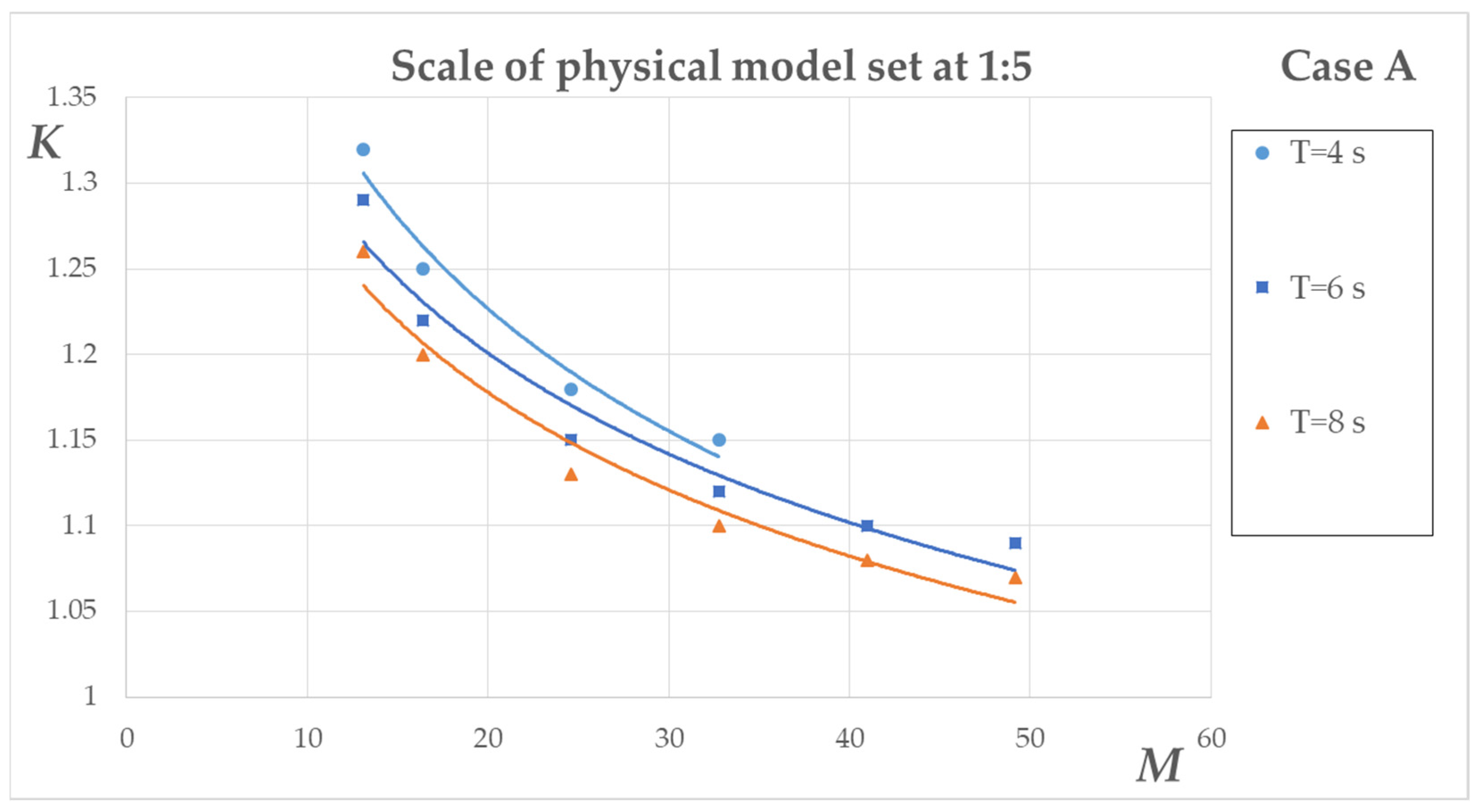
The trend lines with respect to each wave period for Figure 3 are given in Table 6, along with their corresponding coefficients of determination R²; as can be observed, the latter are satisfactory.

Table 6. Trend lines and R² of K–M curves in Figure 3.

R2	Trend Line	T (Sec)
0.967	1.91·M−0.15	4
0.952	1.74·M−0.12	6
0.962	1.70·M−0.12	8

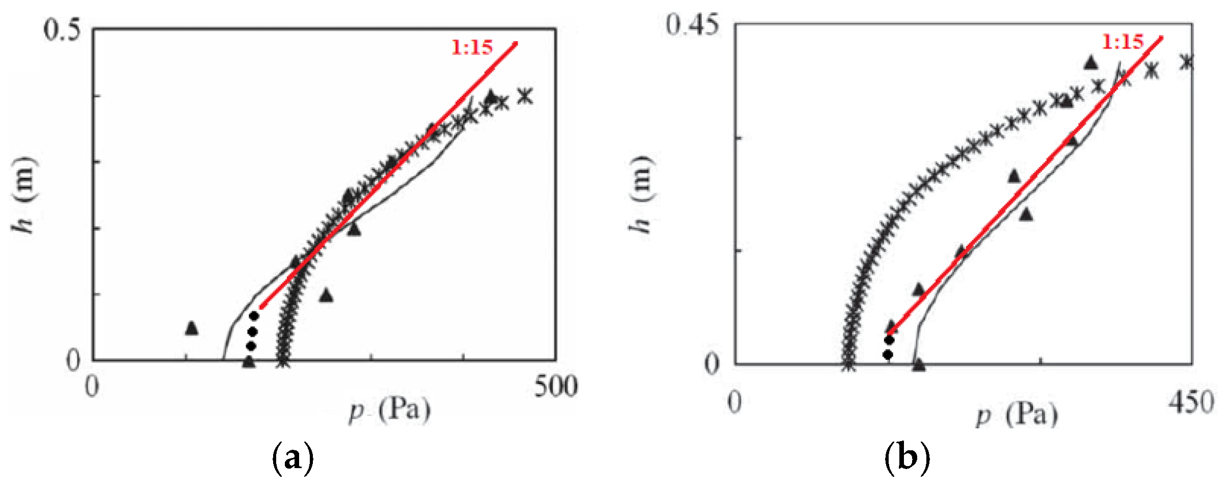
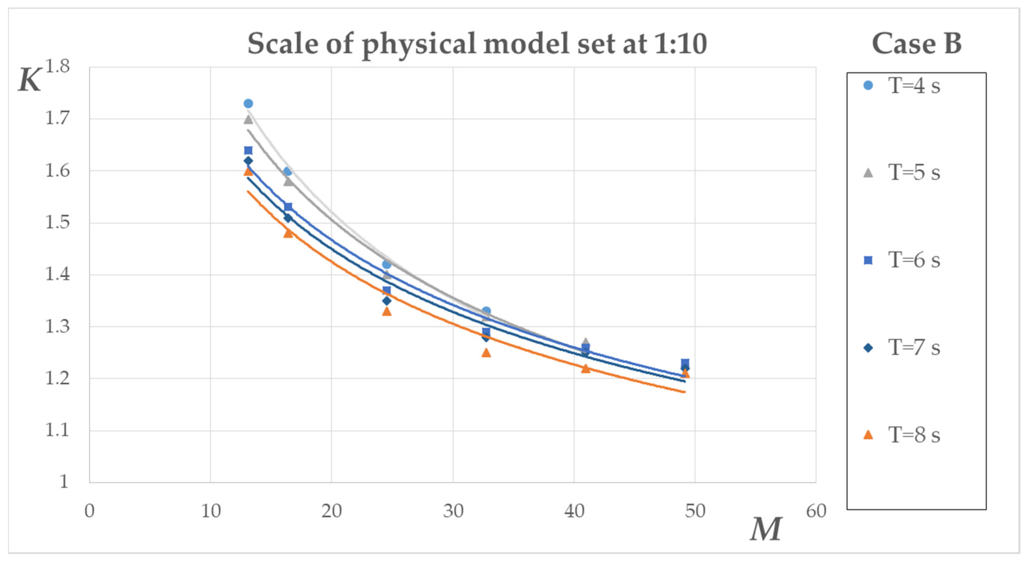
Case B: In Figure 4, the scale correction factor is estimated for a prototype structure with the same core size and sea state as in case A, with the respective physical model set at a scale of 1:10. The abscissa in Figure 4 is calculated in the same way as for case A.

Figure 4. Trend lines of scale correction factor K for a physical model downscaled to 1:10, with prototype conditions of D_n50 = 0.20 m, B = 4.0 m, ΔL = 5.0 m, h_s = 3.0 m, h = 4.0 m, n = 0.4.

The trend lines with respect to each wave period for Figure 4 are given in Table 7, along with their corresponding coefficients of determination R²; as can be observed, again the latter are satisfactory.

Table 7. Trend lines and R² of K–M curves in Figure 4.

R2	Trend Line	T (Sec)
0.994	3.60·M−0.29	4
0.987	3.26·M−0.26	5
0.973	2.83·M−0.22	6
0.969	2.56·M−0.21	7
0.957	2.72·M−0.22	8

Case C: In Figure 5, the scale correction factor is estimated for a prototype structure with the same dimensions and sea state as in case A, except for D_n50 being equal to 0.40 m, with the respective physical model set at a scale of 1:10. The abscissa in Figure 5 is calculated in the same way as for case A.

Figure 5. Trend lines of scale correction factor K for a physical model downscaled to 1:10, with prototype conditions of D_n50 = 0.40 m, B = 4.0 m, ΔL = 5.0 m, h_s = 3.0 m, h = 4.0 m, n = 0.4.

Figure 5. Trend lines of scale correction factor K for a physical model downscaled to 1:10, with prototype conditions of D_n50 = 0.40 m, B = 4.0 m, ΔL = 5.0 m, h_s = 3.0 m, h = 4.0 m, n = 0.4.

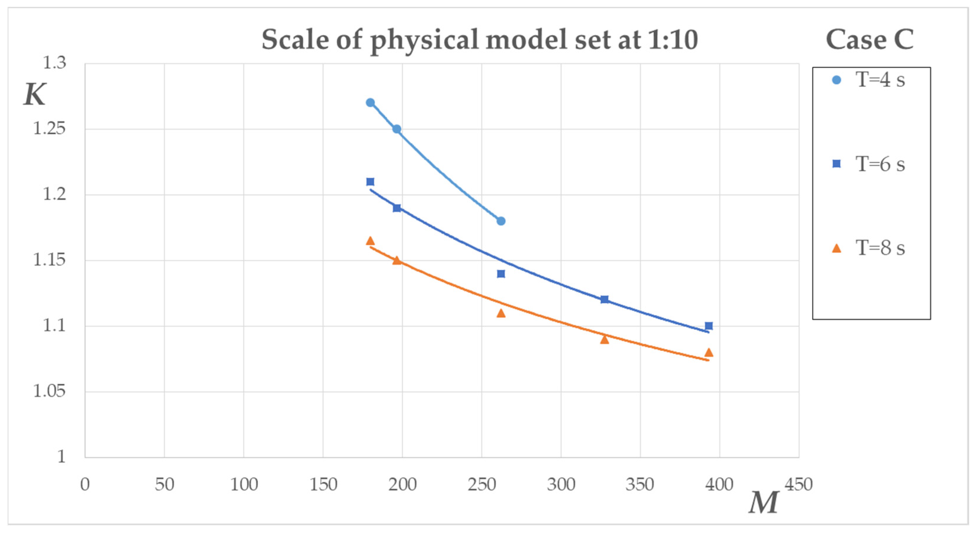
The trend lines with respect to each wave period for Figure 5 are given in Table 8, along with their corresponding coefficients of determination R²; as can be observed, once more, the latter are satisfactory.

Table 8. Trend lines and R² of K–M curves of Figure 5.

R2	Trend Line	T (Sec)
0.999	3.53·M−0.20	4
0.981	2.25·M−0.12	6
0.975	1.94·M−0.10	8

Case D: In Figure 6, the scale correction factor is estimated for a prototype structure with the same dimensions and sea state as in case A, with the respective physical model set at a scale of 1:15. The abscissa of Figure 6 is calculated in the same way as for case A.

Figure 6. Trend lines of scale correction factor K for a physical model downscaled to 1:15, with prototype conditions of D_n50 = 0.20 m, B = 4.0 m, ΔL = 5.0 m, h_s = 3.0 m, h = 4.0 m, n = 0.4.

Figure 6. Trend lines of scale correction factor K for a physical model downscaled to 1:15, with prototype conditions of D_n50 = 0.20 m, B = 4.0 m, ΔL = 5.0 m, h_s = 3.0 m, h = 4.0 m, n = 0.4.

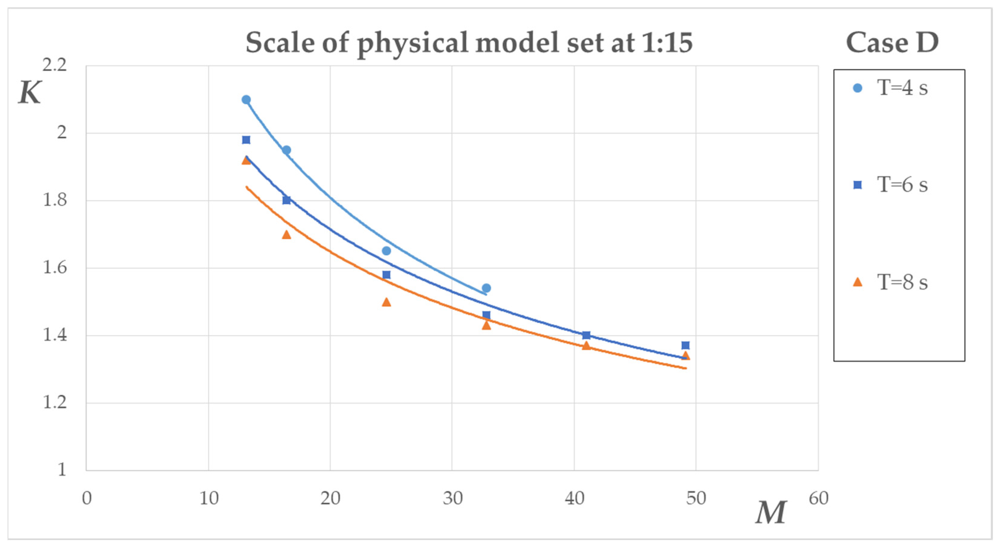
The trend lines with respect to each wave period for Figure 6 are given in Table 9, along with their corresponding coefficients of determination R²; as can be observed, again the latter are satisfactory.

Table 9. Trend lines and R² of K–M curves in Figure 6.

R2	Trend Line	T (Sec)
0.991	5.15·M−0.35	4
0.977	3.80·M−0.28	6
0.951	3.61·M−0.26	8

Further statistical checking of the results presented in the nomographs in Figure 3, Figure 4, Figure 5 and Figure 6 appears to be superfluous, simply because such an investigation would require assuming that the K values shown in the graphs are actual “measured” values. However, this is only partially true, since these values are obtained from equations based on measurements, with both sources introducing a certain amount of uncertainty: the equations due to necessary approximations, and the measurements due to their currently limited availability. For these reasons, no detailed calculation of confidence intervals and other statistical parameters will be presented in order to avoid possible misinterpretation of the results. Instead, a representative case is presented below to demonstrate the very good fit of the regression lines to the calculated K values. Thus, considering the following initial data:

• Power-law function;
• Six raw data sets;
• Mean K = 1.4;
• R² = 0.97;
• Total sum of squares (in ln-space) = 0.1;

• we obtain for centred data (best case) a 95% confidence interval between 1.36 and 1.44, i.e., 2.9% away from the central value. For edge data (worst case), the interval becomes 1.30 to 1.51, i.e., a deviation around 7.5%. For mean K = 1.35 and centred data, the above interval becomes 1.32 to 1.38, i.e., a deviation of 2.2%. It is noted that these confidence intervals cannot represent overall uncertainty of K values for the reasons mentioned above.

Regarding the domain of applicability of the above method for determining the scale correction factor K for the core material size, a certain range of geometries of submerged breakwaters and corresponding sea states were defined. Narrow-crested structures were considered to be more environmentally friendly than wide-crested and emerged mounds. Specifically, the prototype geometrical features were confined to the following:

• Nominal diameter, D_n50, of the core between 0.10 m and 0.50 m;
• Sloping 1:1.5 up to 1:2;
• Crest width, B, between 3.0 m and 6.0 m;
• Structure height, h_s, between 2.5 m and 4.5 m;

• with the following prototype sea state conditions:

• Free board between 0.5 m and 2.0 m;
• Wave period T between 4.0 s and 8.0 s;
• Incident wave height H_i between 0.8 m and 3.0 m.

Extending the above applicability domain is not encouraged until further results on this topic are readily available.

Numerical values behind Figure 3, Figure 4, Figure 5 and Figure 6 are provided in Supplementary Table A1, Table A2, Table A3 and Table A4, given in Appendix A.

7. Discussion

The graphs presented in the previous section provide a satisfactory overview of the main trends related to the central variables of the investigated problem. As mentioned above, the horizontal axis of these graphs was made identical to that used in [4] for ease of comparison with emerged breakwaters. In this latter study, the wave period is not considered as a parameter. As expected, the scale correction factor K is considerably lower for emerged than for submerged breakwaters. For example, for a linear scale of 1:15 and M around 25, K=1.2 for emerged structures according to the nomogram of [4], while K is around 1.55 for submerged mounds according to the methodology presented in Section 6. This difference can be attributed to the different hydrodynamic conditions associated with the two types of breakwater, which result in a steeper pressure gradient in the submerged structure. A further comparison of K values for submerged and emerged structures is presented in Table 10. In general, the ratio of K ranged from 1.3 to 1.6 for the cases examined, with higher K values for the submerged structures.

Table 10. Comparison of K between the proposed method for submerged mounds and the method by Le Méhauté [4] for emerged mounds and T = 4 s, D₅₀ = 0.20 m, ΔL = 5 m, under a scale of 1:15.

	Submerged Mound	Emerged Mound
Hi (m)	K	K	K-Ratio
0.8	2.10	1.35	1.55
1.0	1.95	1.25	1.56
1.5	1.65	1.20	1.38
2.0	1.54	1.00	1.54

It is also noticed that increasing the adopted linear scale of the physical model tends to require lower correction regarding the size of the core material. Indeed, for M around 30, the nomographs of Figure 3, Figure 4 and Figure 6 give central values of the scale correction factor K of around 1.15, 1.3 and 1.5 for scales of 1:5, 1:10 and 1:15, respectively. This is because smaller models lead to a finer model material and smaller pore sizes, inducing more pronounced deviations from the prototype flow conditions. The same reasoning explains the decreasing trend in K with increasing D_n50, or equivalently with increasing M, with all other parameters kept constant, as observed in all the above nomographs.

The effects of stone shape and packing mode on the porosity and the Forchheimer coefficients have been studied in the past (see, for example, [31]), with porosity n being a principal variable associated with most of the mentioned stone properties. On the other hand, it can be seen that the resistance coefficients, given by Equations (3), (4), and (8), are indeed sensitive to porosity. In the applications presented above, typical stone conditions were assumed so that the results would be more widely applicable. Inspection of Figure 3, Figure 4, Figure 5 and Figure 6, where M ~ n⁵, reveals that, with all other variables kept constant, an increase in the prototype porosity leads to a decrease in K values, as expected. Specifically, Table 11 shows the variation in actual K values over a realistic range of n for a typical geometry of submerged structures (B = 4.0 m, ΔL = 5 m, h_s = 4.0 m and h = 5.0 m) and representative wave conditions.

Table 11. Scale correction factor K for a physical model downscaled to 1:10, with prototype conditions of D_n50 = 0.20 m, T = 6 s, over a band of porosity values and wave heights.

K
n = 0.52	n = 0.49	n = 0.46	n = 0.43	n = 0.4	Hi (m)
1.41	1.44	1.49	1.55	1.64	0.8
1.34	1.38	1.43	1.45	1.53	1
1.21	1.25	1.29	1.32	1.37	1.5
1.15	1.19	1.23	1.27	1.29	2
1.14	1.15	1.19	1.23	1.26	2.5
1.13	1.13	1.15	1.19	1.23	3

The expected behaviour of K as related to n, i.e., for higher n we should expect lower K, is clearly confirmed by the representative data in Table 11.

A final remark on the results concerns the influence of the wave period T on the correction factor K applied to the core material scaling. It can be seen that an increase in T leads to slightly lower K values, with all other parameters kept fixed. The reason for this is that the b term of the Forchheimer Equation (1) decreases as the KC number increases, owing to the increase in T; hence, the balance between the a and b terms shifts in favour of the laminar part of the flow, which generally requires a smaller scale correction for the model core.

The numerical applications given in the previous section can serve as examples of how to determine the correction factor for the scaling of the small-size material in physical models of submerged sloping breakwaters. The user can employ either the set of equations proposed in this article or the nomographs provided. The latter approach is considerably easier and faster and may therefore be preferred, especially when the data for the examined case fall close to those represented by the nomographs. However, it should be underlined that the K values presented previously should be used primarily as preliminary engineering estimates until full validation is achieved in future research.

The presented application used a spatial simplification whereby a single path of the maximum δp/δx values was followed along the mean distance between the two parallel sides of the trapezoidal shape of the breakwater. This approach could be applied multiple times to solve the extended Forchheimer equation in parallel zones, into which the cross-section of the structure can be divided in the cross-sectional horizontal direction; the results should then be averaged to give a single answer. Initial results on this issue show an insignificant variation in the final K value. This is due to the linear dependence between K and ΔL, which can be attributed to the fact that a representative hydrodynamic pressure gradient in the offshore half of the structure is a linear function of ΔL for the purposes of the present application method. An example of results obtained for three parallel zones within the same cross-section is given in Table 12, showing that the use of the middle zone alone gives the same K as that obtained by averaging the results from the three zones.

Table 12. Sensitivity analysis of K given for a wave of T = 6.0 s and H_i ranging from 0.8 m up to 3.0 m, with respect to ΔL for a scale 1:10, prototype core D_n50 = 0.20 m and n = 0.4.

6	5	4	ΔL (m)
K			Hi (m)
1.7	1.64	1.59	0.8
1.55	1.49	1.45	1
1.38	1.35	1.33	1.5
1.32	1.29	1.27	2
1.28	1.26	1.23	2.5
1.25	1.23	1.21	3

Additionally, the formulation developed in Section 4 uses coefficients that involve parameters like D_n50, the KC number, etc., so that the conventional check on the flow conditions through evaluation of the Reynolds or Keulegan–Carpenter numbers becomes less critical. Also, the transition from laminar to turbulent flow has been smoothened through the inclusion of an extra term on the right-hand side of the extended Forchheimer equation (see the relevant factor in Equation (8)).

As indicated by previous research (see refs. [19,20]), wave breaking does not play a significant role in the pressure gradient inside the porous medium. Regarding the incoming wave type, it was found that the use of regular waves is advisable for controlled derivation or calibration, since the definition of the maximum velocity values needed to feed the Forchheimer equation is more straightforward for regular waves than for random waves.

The results presented in this paper are based on experiments with homogeneous structures. However, if an armour layer is formed by a different material, it can be accepted that the pressure on the slope of the structure can retain the same value over a section of the armour layer measured along the horizontal, due to the typically larger pores present in that layer. The width of that section can be defined through future research on multilayer submerged breakwaters. However, it is suggested that, for most practical applications, i.e., within the scope of this study and under typical conditions, the outer one-stone layer would have an insignificant effect on pore-pressure modification. In cases with extra sublayers and filter layers, a piecewise application of the mathematical model given previously can be carried out.

8. Conclusions

This paper presents original results on the required scale correction to be applied to the size of the core material in physical models of submerged rubble-mound breakwaters, so that prototype internal hydraulics may be more credibly reproduced in those models. The case of submerged mounds has not been examined so far, in contrast to their emerged counterparts. The hydrodynamic field around and inside these two porous structure types under wave action differs considerably. The results of the present work on the sizing of the core material show considerable deviations from the corresponding results for emerged structures, thus justifying the scope of this investigation, which is based on widely accepted maritime hydrodynamics and porous flow theory. Another factor in support of this research is the increasing presence of submerged breakwaters in coastal management projects, due to their potential to foster marine life.

Further, a specific innovation developed by others was introduced here in the development of the extended Forchheimer equation, namely a new term in that equation to account for a smooth transition from the laminar to the turbulent flow state.

Future research on this issue could involve the use of more raw data to validate K values and expand the range of applicability of the current results pertaining to the downscaling correction of submerged breakwaters. Also, the extension to multi-layer structures requires further development and validation.

References

- Sutton-Grier, A.E.; Wowk, K.; Bamford, H. Future of our coasts: The potential for natural and hybrid infrastructure to enhance the resilience of our coastal communities, economies and ecosystems. Environ. Sci. Policy 2015, 51, 137–148. [Google Scholar] [CrossRef] [Scilit]
- Dalrymple, R.A. Introduction to physical models in coastal engineering. In Physical Modelling in Coastal Engineering; Dalrymple, R.A., Ed.; A.A. Balkema: Rotterdam, The Netherlands, 1985. [Google Scholar]
- Hughes, S.A. Physical Models and Laboratory Techniques in Coastal Engineering; Advanced Series on Ocean Engineering; World Scientific Publishing: Singapore, 1993; Volume 7, 568p. [Google Scholar]
- Méhauté Le, B. Wave Absorbers in Harbors; Contract Report No. 2-122; US Army Engineer Waterways Experiment Station: Vicksburg, MI, USA, 1965. [Google Scholar]
- Keulegan, G.H. Wave Transmission Through Rock Structures; Research Report H-73-1; US Army Engineer Waterways Experiment Station: Vicksburg, MI, USA, 1973. [Google Scholar]
- Hudson, R.Y.; Herrmann, F.A.; Sager, R.A.; Whalin, R.W.; Keulegan, G.H.; Chatman, C.E.; Hales, L.Z. Coastal Hydraulic Models; Special Report no 5; US Army Engineer Waterways Experiment Station: Vicksburg, MI, USA, 1979. [Google Scholar]
- Gu, Z.; Wang, H. Gravity waves over porous bottoms. Coast. Eng. 1991, 15, 497–524. [Google Scholar] [CrossRef] [Scilit]
- van Gent, M.R.A. Stationary and Oscillatory Flow Through Coarse Porous Media; Communications of Hydraulic and Geotechnical Engineering, Report No 93-9; Delft University of Technology: Delft, The Netherlands, 1993. [Google Scholar]
- Losada, I.J.; Losada, M.A.; Martin, A. Experimental study of wave-induced flow in a porous structure. Coast. Eng. 1995, 26, 77–98. [Google Scholar] [CrossRef] [Scilit]
- Tirindelli, M.; Lamberti, A.; Paphitis, D.; Collins, M.; Vidal, C.; Hawkins, S.; Moschella, P.; Burcharth, H.; Sánchez-Arcilla, A. Wave Action on Rubble Mound Breakwaters: The Problem of Scale Effects; DELOS Report D52, Hydraulic Engineering Reports; Delft University of Technology: Delft, The Netherlands, 2004. [Google Scholar]
- Troch, P.; De Rouck, J.; Burcharth, H.F. Experimental study and numerical modeling of wave induced pore pressure attenuation inside a rubble mound breakwater. In Proceedings of the International Conference on Coastal Engineering, Cardiff, UK, 7–12 July 2002; pp. 1607–1619. [Google Scholar]
- Muttray, M.; Oumeraci, H. Theoretical and experimental study on wave damping inside a rubble mound breakwater. Coast. Eng. 2005, 52, 709–725. [Google Scholar] [CrossRef] [Scilit]
- Cantelmo, C.; Allsop, W.; Dunn, S. Wave pressure in and under rubble mound breakwaters. In Proceedings of the Third International Conference on the Application of Physical Modelling to Port and Coastal Protection, Barcelona, Spain, 28 September–1 October 2010. [Google Scholar]
- Vanneste, D.; Troch, P. An improved calculation model for the wave-induced pore pressure distribution in A rubble-mound breakwater core. Coast. Eng. 2012, 66, 8–23. [Google Scholar] [CrossRef] [Scilit]
- Guance, R.; Iturrioz, A.; Losada, I.J. Hybrid modeling of pore pressure damping in rubble mound breakwaters. Coast. Eng. 2015, 99, 82–95. [Google Scholar] [CrossRef] [Scilit]
- Tomasicchio, G.R.; Mahmoudi Kurdistani, S. New prediction formula for pore pressure distribution inside rubble-mound breakwater. J. Waterw. Port Coast. Ocean Eng. 2020, 146, 04020005. [Google Scholar] [CrossRef] [Scilit]
- Scaravaglione, G.; Marino, S.; Francone, A.; Damiani, L.; Tomasicchio, G.R.; Saponieri, A. Laboratory investigation on pore pressures inside a rubble mound breakwater in depth-limited waters. Appl. Ocean Res. 2024, 147, 103988. [Google Scholar] [CrossRef] [Scilit]
- Garcia, N.; Lara, J.L.; Losada, I.J. 2-D numerical analysis of near-field flow at low-crested permeable breakwaters. Coast. Eng. 2004, 51, 991–1020. [Google Scholar] [CrossRef] [Scilit]
- Metallinos, A.; Emmanouilidou, M.-E.; Memos, C.D. Wave-induced pore pressures in submerged rubble mound breakwaters simulated by a compound Boussinesq model. J. Hydraul. Res. 2014, 52, 24–35. [Google Scholar] [CrossRef] [Scilit]
- Roupas, I. Study of Turbulent Pressures and Wave Transmission Coefficient at Submerged Permeable Breakwaters. Master’s Thesis, National Taiwan University of Arts, Taipei, Taiwan, 2019. [Google Scholar]
- van Gent, M.R.A. Porous Flow through Rubble-Mound Material. J. Waterw. Port Coast. Ocean Eng. 1995, 121, 176–181. [Google Scholar] [CrossRef] [Scilit]
- Burcharth, H.F.; Andersen, O.K. On the one-dimensional steady and unsteady porous flow equations. Coast. Eng. 1995, 24, 233–257. [Google Scholar] [CrossRef] [Scilit]
- Losada, I.J.; Lara, J.L.; del Jesus, M. Modeling the Interaction of Water Waves with Porous Coastal Structures. J. Waterw. Port Coast. Ocean Eng. 2016, 142, 03116003. [Google Scholar] [CrossRef] [Scilit]
- Vanneste, D.; Troch, P. Improvements to the core scaling method for rubble-mound breakwaters. In Proceedings of the Fourth International Conference on the Application of Physical Modelling to Port and Coastal Protection (Coastlab12), Ghent, Belgium, 17–20 September 2012. [Google Scholar]
- Polubarinova-Kochina, P. Theory of Groundwater Movement; Princeton University Press: Princeton, NJ, USA, 1962. [Google Scholar]
- van Gent, M.R.A. Formulae to Describe Porous Flow. Commun. Hydraul. Geotech. Eng. 1992, 92, 50. [Google Scholar]
- Jensen, B.; Jacobsen, N.G.; Christensen, E.D. Investigation on the porous media equations and resistance coefficients for coastal structures. Coast. Eng. 2014, 84, 56–72. [Google Scholar] [CrossRef] [Scilit]
- Lara, J.L.; Losada, I.J.; Maza, M.; Guanche, R. Breaking solitary wave evolution over a porous underwater step. Coast. Eng. 2011, 58, 837–850. [Google Scholar] [CrossRef] [Scilit]
- Lin, P.; Karunarathna, S. Numerical study of solitary wave interaction with porous breakwaters. J. Waterw. Port Coast. Ocean Eng. 2007, 133, 352–363. [Google Scholar] [CrossRef] [Scilit]
- Avgeris, I.; Karambas, T.V.; Prinos, P. Boussinesq modeling of wave interaction with porous submerged breakwaters. In Proceedings of the 29th International Conference on Coastal Engineering, Lisbon, Portugal, 19–24 September 2004; McKee Smith, J., Ed.; World Scientific: Singapore, 2004; pp. 604–616. [Google Scholar]
- Burcharth, H.F.; Liu, Z.; Troch, P. Scaling of core material in Rubble Mound Breakwater Model Tests. In Proceedings of the Fifth International Conference on Coastal and Port Engineering in Developing Countries COPEDEC V, Cape Town, South Africa, 19–23 April 1999; pp. 1518–1528. [Google Scholar]
Disclaimer/Publisher’s Note: The statements, opinions and data contained in all publications are solely those of the individual author(s) and contributor(s) and not of MDPI and/or the editor(s). MDPI and/or the editor(s) disclaim responsibility for any injury to people or property resulting from any ideas, methods, instructions or products referred to in the content. |
© 2026 by the authors. Licensee MDPI, Basel, Switzerland. This article is an open access article distributed under the terms and conditions of the Creative Commons Attribution (CC BY) license.