


Abstract
As a key component for perception of the environment and structural response, the normal operation of sensors is crucial for the safety assessment of pipe-rack offshore platforms. However, in long-term service, sensors on the jacket platform are susceptible to high salt-spray corrosion and strong vibration in marine environments, which can lead to bias, drift, accuracy degradation, gain anomaly, and stuck-at faults. These fault signals can mask real structural damage and cause misjudgment. The existing temporal diagnosis models have difficulty in simultaneously capturing long-range dependencies and the local dynamic evolution in temporal data. Therefore, this paper proposes to construct a sensor fault diagnosis model based on the parallel fusion of a Temporal Convolutional Network (TCN) and Gated Recurrent Unit (GRU). First, five types of sensor fault mathematical models were established, and 10 composite fault conditions were constructed. Second, a dual branch parallel architecture was designed, using sliding windows and time-domain expansion to construct the time-series dataset. The TCN branch relies on causal and dilated convolution to capture the long-term dependencies of signals, while the GRU branch extracts local dynamic evolution features through a dual gate control mechanism. The TCN and GRU branches extract features in parallel and fuse them to complete fault classification. On a numerical model of a pipe-rack offshore platform containing seven triaxial acceleration sensors, this method achieved an accuracy of 97.34% in diagnosing 10 types of composite faults, significantly better than single TCN (89.2%) and single GRU (84.8%). The confusion matrix display can effectively distinguish even when encountering fault types with similar characteristics such as drift + stuck composite faults. In the scaled-model physical experiment, the TCN-GRU sensor fault diagnosis model is validated on a ten-class composite fault dataset constructed by superimposing five types of mathematically synthesized sensor faults onto measured healthy signals collected from a laboratory-scale model (not naturally occurring sensor faults), and achieves an accuracy of 91.18%. This study focuses on the sensor fault diagnosis of offshore platforms with pipeline racks under the influence of typhoons, and proposes an intelligent sensor fault diagnosis model based on TCN-GRU parallel fusion. At the same time, the model was validated through scaled physical experiments, as an auxiliary check to verify the effectiveness of the experimental platform and data-acquisition system.
1. Introduction
As an important component of the national energy strategy, ocean energy development has been continuously advancing towards deep and distant seas in recent years [1,2,3]. As the core infrastructure for fixed offshore and deepwater oil and gas extraction, offshore platforms of pipeline racks have been in service for a long time in extremely harsh marine environments. Under extreme conditions such as typhoons, platform structures are frequently subjected to the coupling effects of strong winds, huge waves, and complex ocean currents, bearing enormous dynamic loads and high-frequency vibrations [4,5,6]. To monitor the service status and structural safety of the platform in real time, it is necessary to deploy a large number of multidimensional acceleration sensors on its key components and nodes to construct a structural health monitoring system. However, the comprehensive factors such as high salt-spray corrosion, temperature and humidity cycling, electromagnetic interference, and strong vibration fatigue in the oceanic atmospheric zone can easily lead to the degradation or sudden failure of sensitive sensor components, inducing various typical faults such as deviation, drift, accuracy degradation, gain abnormalities, and jamming. Distorted or failed sensor systems cannot accurately reflect the true structural dynamic response of the platform; worse, they may mask real structural damage and even cause false or missed alarms, thereby seriously threatening the safe operation of offshore oil and gas facilities. In addition to the health monitoring of the offshore platform itself, the integrity inspection of subsea pipelines connected to the platform is also a critical safety issue that deserves attention in marine oil and gas engineering [7,8].
At present, in the research of sensor fault diagnosis on offshore platforms, traditional fault identification methods mainly rely on analytical redundancy methods based on physical mechanism models, as well as measurement verification systems built on hardware redundancy [9,10,11,12]. However, under the extremely variable and strong nonlinear dynamic loads of typhoons, the platform structure response is complex, it is difficult for traditional analytical redundant models to accurately characterize the complex environmental excitation and structural coupling relationship. With the vigorous development of artificial intelligence and deep learning technology, data-driven temporal intelligent diagnostic methods have shown great potential in the field of structural health monitoring [13,14,15,16]. Convolutional neural networks (CNNs) and recurrent neural networks (RNNs and their variant LSTMs and GRUs) are widely used for feature extraction and classification of temporal signals [17,18,19]. However, a single convolutional architecture (such as standard TCN) can capture long-range dependencies through causal convolution and dilation convolution when facing complex non-stationary dynamic responses of ocean platforms, but often lacks precise capture of local transient evolution characteristics. A single RNN (such as GRU) is good at handling sequence dynamics, but it is susceptible to gradient vanishing and to insufficient local feature representation when trained on long sequences. Especially in typhoon environments, complex composite faults often occur between multiple measurement points and sensors, and different fault modes exhibit highly similar feature coupling. This makes it difficult for existing time-series diagnostic models to simultaneously consider the deep extraction of long-range time-series dependencies and local dynamic evolution information, and to meet the urgent needs of complex marine engineering for high reliability and high-precision fault diagnosis.
In response to the limitations of existing single temporal diagnostic models in capturing both long-range signal evolution patterns and local abrupt features in complex sea conditions, scholars at home and abroad have conducted extensive research on temporal feature fusion and deep learning architecture optimization. Multi-scale feature fusion and hybrid neural network architectures have gradually become cutting-edge hotspots in the field of intelligent diagnosis due to their ability to effectively integrate the structural advantages of different algorithms. For example, combining convolutional structures with recurrent gating units that are adept at handling time-step dependencies can theoretically achieve the organic unity of global trend characterization and local dynamic perception [20,21]. However, most existing hybrid models adopt a serial stacking structure, which often encounters bottlenecks such as temporal information loss and single-feature expression in the process of deep information transmission. Especially in the harsh environment of multiple measurement points, high noise, and highly overlapping composite fault features on offshore platforms, their robustness and discrimination accuracy are still insufficient. In addition, traditional hybrid architectures often overlook the inherent correlation between multi-channel sensor spatial responses when dealing with non-stationary time series, making it difficult to separate the coupling effects of environmental noise and real fault signals in complex feature spaces. Therefore, when facing multi-sensor composite faults, such architectures are prone to misjudgment or omission, which cannot provide accurate warnings for the safety assessment of the main structure [22,23,24].
Based on this, this article takes the offshore platform of a pipeline rack under a typhoon environment as the research object, and constructs an intelligent sensor fault diagnosis model based on the parallel fusion of TCN and GRU. First, the system establishes five typical fault mathematical models for sensors, including deviation, drift, accuracy degradation, gain, and jamming. Based on finite element numerical simulation and multidimensional measurement point response data, a standard dataset covering 10 complex multi-sensor composite fault conditions is constructed. Second, we design a dual-branch parallel fusion architecture. The TCN branch relies on causal convolution and dilation convolution to capture the long-range temporal dependencies and global evolution trends of signals, while the GRU branch extracts local dynamic evolution features and transient mutation details through a dual-gate control mechanism of reset and update gates. The two branches output lossless concatenation fusion and global average pooling in the feature dimension, achieving complementary advantages of long-period gradient features and instantaneous abnormal features. Although the TCN and GRU modules themselves are established temporal feature extractors, the dual-branch parallel concatenation fusion scheme is the novel design proposed in this work. Finally, the diagnostic performance of the proposed method was systematically validated through numerical modeling and model experiments. The research findings of this article provide theoretical support for the health-status assessment of offshore platforms. It should be noted that the core research content of this article is sensor fault diagnosis. CNN ResNet structural damage diagnosis is only used as an auxiliary verification link in physical experiments to test the effectiveness of the experimental platform and data acquisition system, and is not the main research object of this study.
To systematically sort out existing research achievements on intelligent sensor fault diagnosis for offshore platforms and clarify the novelty of this study, a structured literature search was carried out across Web of Science Core Collection, ScienceDirect and CNKI using combined search keywords including offshore platform, sensor fault diagnosis, time-series deep learning, hybrid fusion network and their Chinese counterparts. Peer-reviewed journal and conference papers published from 2010 to 2025 focusing on offshore-platform-related or time-series-based fault diagnosis were included, while dissertations, book chapters, conference abstracts and studies irrelevant to marine-engineering sensor-fault diagnosis or without fault-identification tasks were excluded. Initial records obtained from database searching were first screened by title and abstract, and remaining highly relevant papers were further evaluated by full-text reading to build the reference library. Existing offshore-platform sensor-fault-diagnosis approaches can be grouped into analytical-redundancy mechanism-based methods, signal-processing-driven feature-engineering methods, and data-driven deep-learning methods. Analytical-redundancy methods require high-fidelity physical models and are difficult to apply under complex non-stationary wind-wave-current coupled typhoon conditions with limited generalization capability. Signal-processing-based methods rely on manually designed fault features and show poor performance for multi-measurement-point coupled compound faults. In time-series deep-learning research, TCN captures long-range temporal dependencies and GRU extracts local transient dynamic features. However, most existing hybrid temporal networks adopt serial-stack fusion, which may lead to temporal information decay during layer-by-layer feature propagation and degrade recognition performance for heavily aliased multi-sensor compound faults. Against such limitations, this paper constructs a dual-branch TCN-GRU parallel fusion architecture, where two branches extract features independently before feature-dimension concatenation fusion to avoid serial-propagation-caused information loss and improve diagnosis accuracy for offshore-platform multi-sensor compound faults.
The main contributions of this paper are as follows.
(1) Aiming at the coexistence of slow evolution and transient abrupt change in sensor faults of jacket platforms under typhoon conditions, a TCN-GRU dual-branch parallel fusion diagnosis model is proposed, in which the TCN branch captures long-range temporal dependencies and the GRU branch extracts local dynamic evolution features. The two branches extract features in parallel and fuse them along the feature dimension, avoiding the temporal information loss of serial structures.
(2) Five types of sensor fault mathematical models are established, and a dataset containing 10 composite multi-sensor fault conditions is constructed.
2. Materials and Methods
2.1. Basic Theoretical Background
2.1.1. Fault Cause Analysis
Under the influence of typhoons, offshore platforms with pipeline racks have been operating in complex marine environments for a long time, and their sensor systems face the comprehensive impact of multiple fault factors. The high salt-spray concentration and temperature and humidity cycling in the oceanic atmospheric zone continue to affect the sensitive components of the sensors, leading to material interface oxidation and electrochemical corrosion. The high-frequency vibration and instantaneous impact generated by the strong wind and wave loads of typhoons can cause displacement of sensor structures or fatigue damage to components [25]. The electromagnetic pulse of the radar system in the electromagnetic environment around the platform is transmitted through the interference signal link. The sensor installation position is not firmly fixed or is calibrated incorrectly, causing dynamic response distortion. The voltage fluctuation of the power system and the high wind speed and humidity under extreme weather conditions further weaken the stability of sensors. Material defects and external physical impacts during the manufacturing process can directly cause sensor performance degradation or sudden failure due to falling objects during construction. Because these factors exist in the marine environment, they can reduce the reliability of sensor monitoring. The following table (Table 1) shows common types of sensor faults and their causes.
Table 1.
Common Sensor Fault Types and Their Causes.
2.1.2. Fault Mathematical Model
A mathematical model is constructed for sensor faults by mathematically modeling fault modes such as deviation, drift, accuracy degradation, gain, and jamming, converting normal sensor signals into synthetic signals with specific fault characteristics, and providing effective data for intelligent diagnosis [26,27,28,29,30]. This study adopts constant and linearly varying fault parameters and only simulates five basic fault types—bias, drift, precision degradation, gain anomaly, and stuck-at faults—while complex fault forms that may actually occur in offshore sensors, such as intermittent jumps and nonlinear time-varying degradation, have not yet been considered.
The mathematical equations for common types of faults are shown in Table 2. A Gaussian white noise sequence represents simulated environmental noise, representing the standard deviation of the sensor timing signal. The fault adjustment parameters are divided into low-intensity parameters and high-intensity parameters.
Table 2.
Mathematical Equations for Common Fault Types.
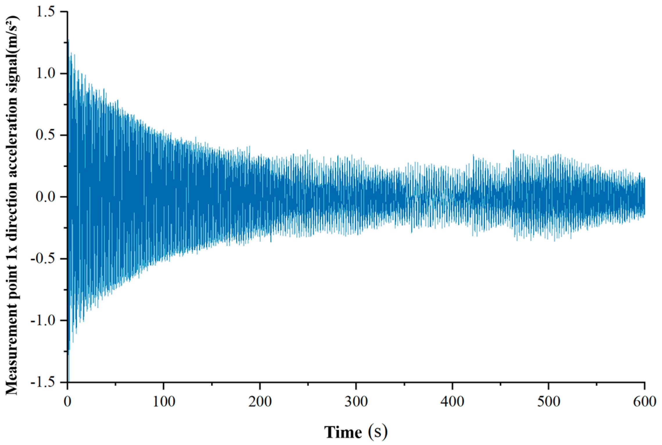
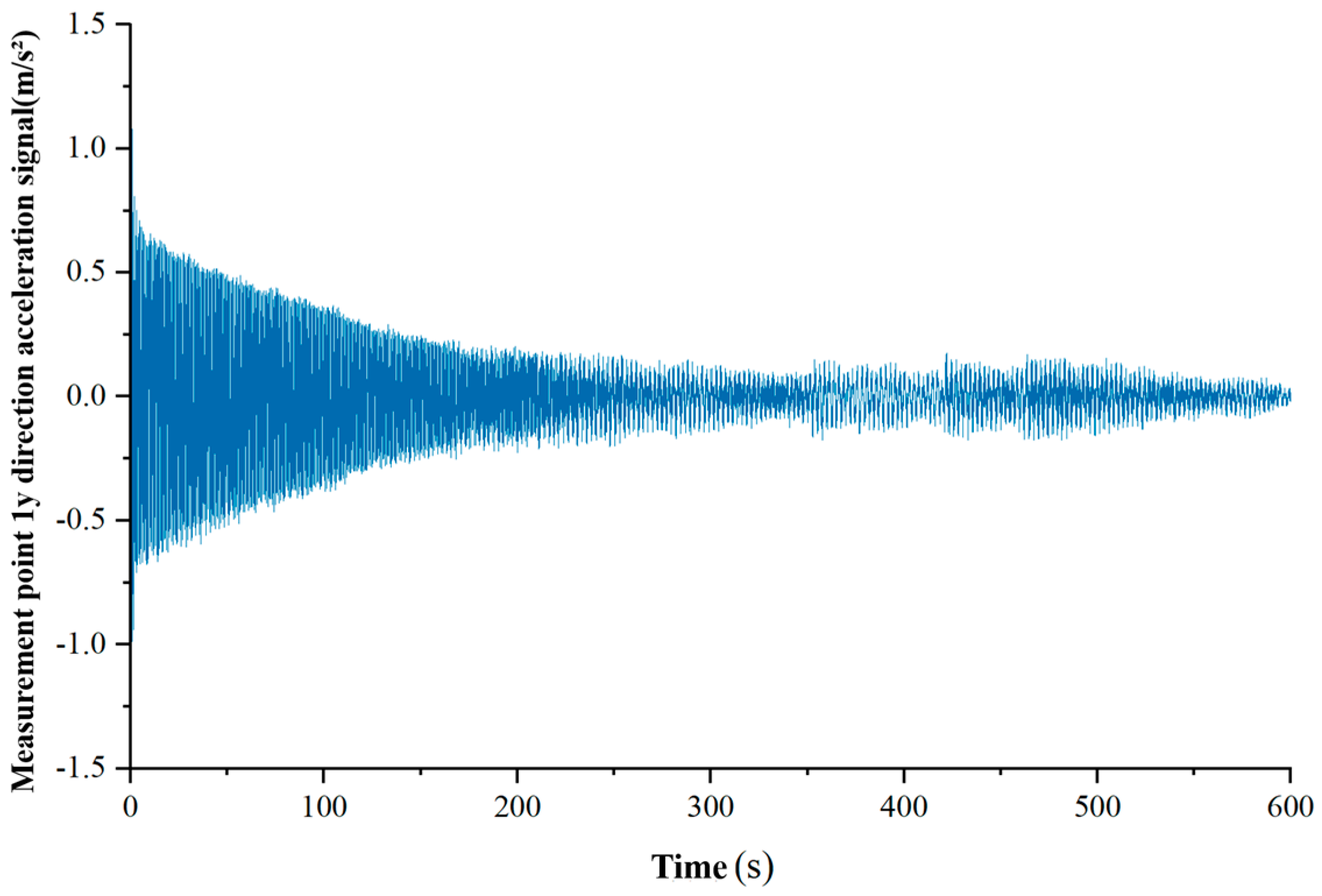
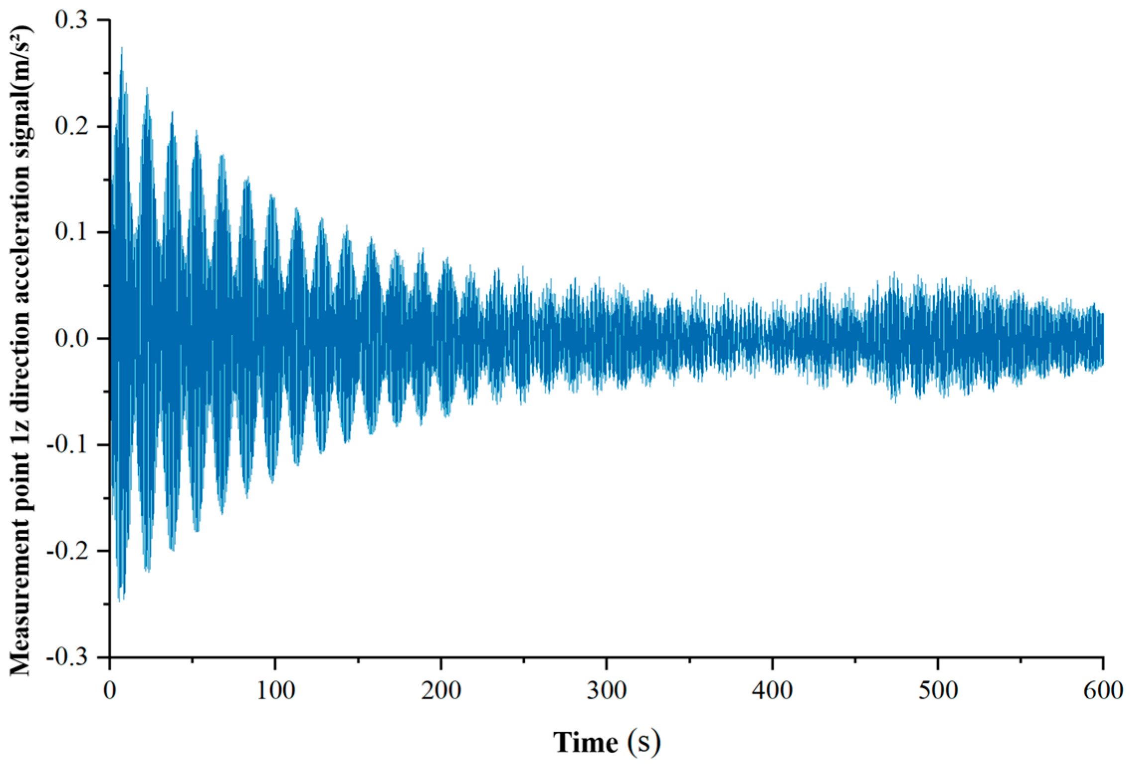
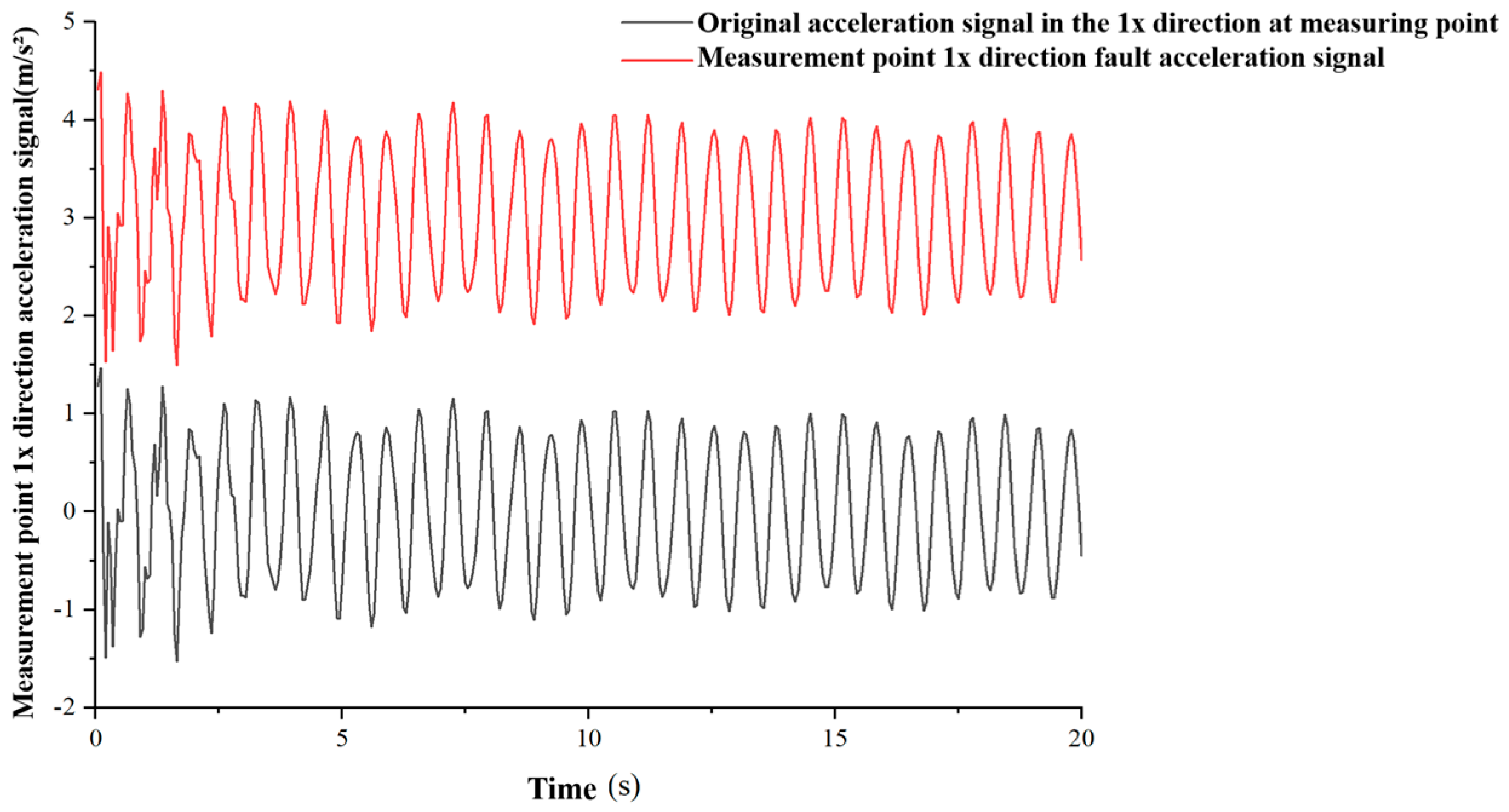
In order to explore the intelligent diagnosis method for sensor faults on a jacket platform under extreme sea conditions of typhoons, this paper is based on a finite element model of the platform structure and a multi-sensor monitoring system. By applying wave, current and typhoon loads, acceleration response time history data of the jacket platform under various typical working conditions are collected. The data for the figures in Section 2.1.2 are obtained from ABAQUS finite-element simulation, and the fault signals are calculated according to the mathematical model of sensor faults in Section 2.1.2.
The normal acceleration signal in the 1x direction of the measuring point is shown in the following Figure 1.
Figure 1.
Acceleration signal in the 1x direction at measuring point 1.
The normal acceleration signal in the direction of measurement point 1y is shown in the following Figure 2.
Figure 2.
Acceleration signal in the 1y direction at measuring point 1.
The normal acceleration signal in the 1z direction of the measuring point is shown in the following Figure 3.
Figure 3.
Acceleration signal in the 1z direction at measuring point 1.
The following Figure 4 shows the comparison between the deviation fault signal generated based on the sensor fault mathematical model and the original normal signal of the acceleration signal in the 1x direction of the measuring point.
Figure 4.
Comparison between deviation fault signal and original normal signal.
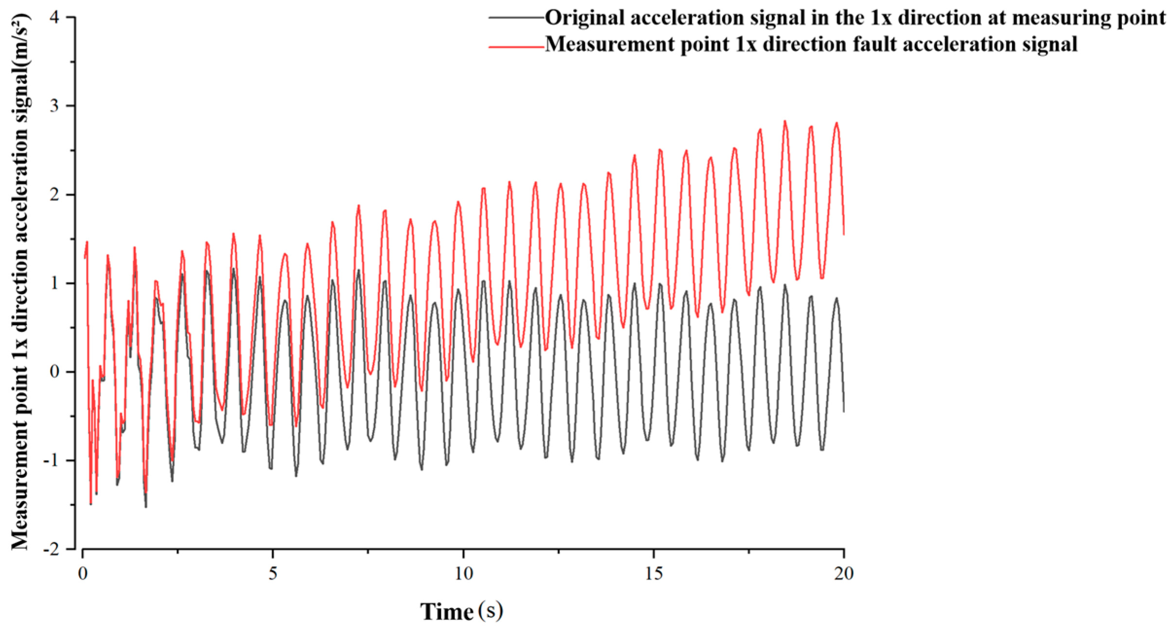
The following Figure 5 shows the comparison between the drift fault signal generated based on the sensor fault mathematical model and the original normal signal of the acceleration signal in the 1x direction of the measuring point.
Figure 5.
Comparison between drift fault signal and original normal signal.
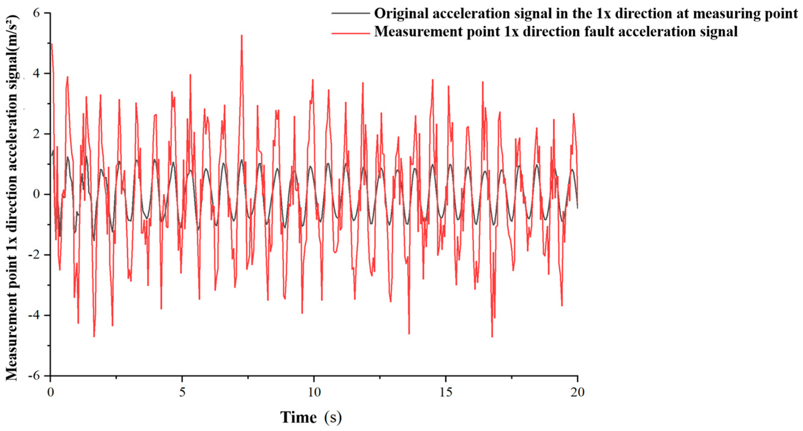
The following Figure 6 shows the comparison between the accuracy degradation fault signal generated based on the sensor fault mathematical model of the acceleration signal in the 1x direction of the measuring point and the original normal signal.
Figure 6.
Comparison between accuracy degradation fault signal and original normal signal.
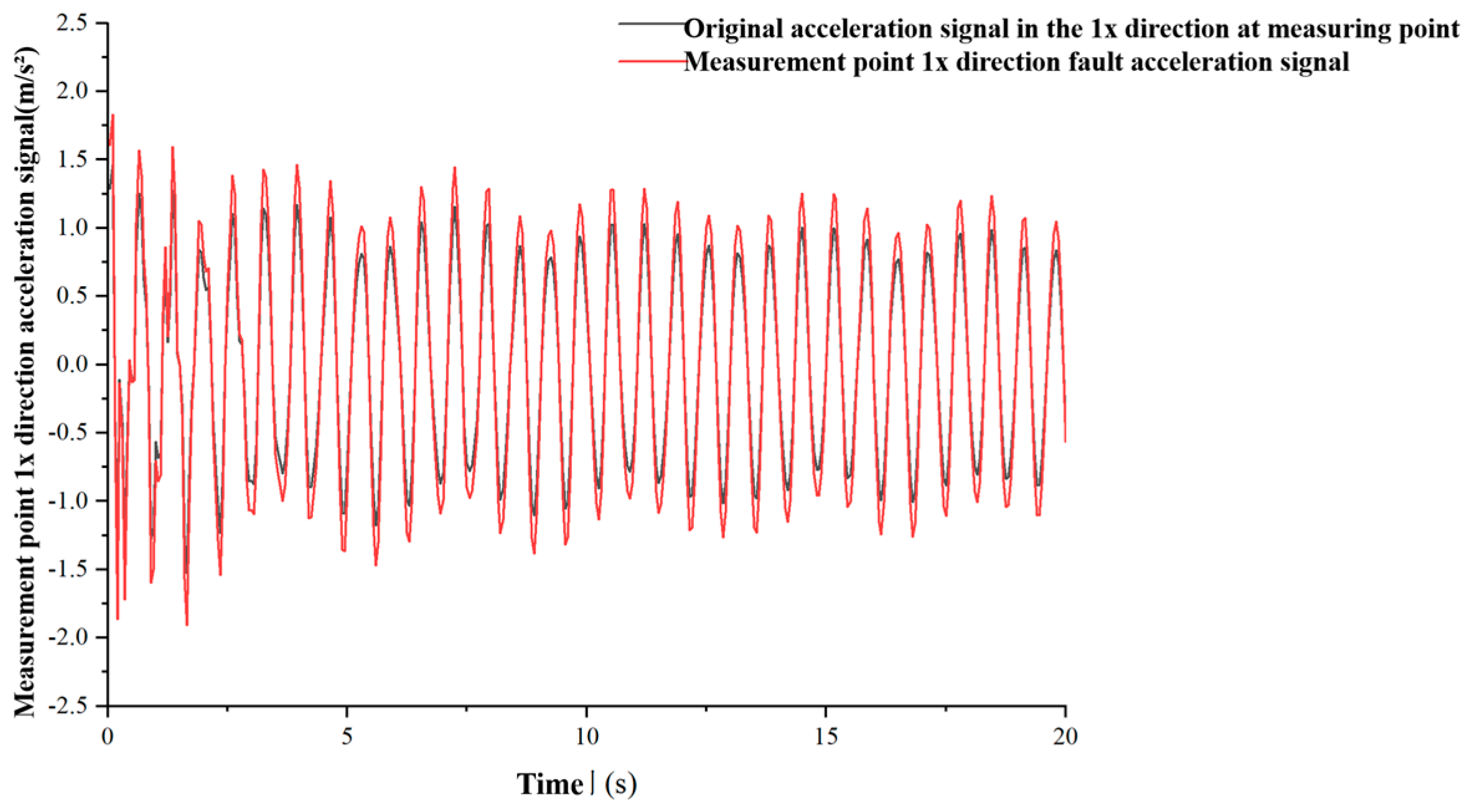
The following Figure 7 shows the comparison between the gain fault signal generated based on the sensor fault mathematical model and the original normal signal of the acceleration signal in the 1x direction of the measuring point.
Figure 7.
Comparison between gain fault signal and original normal signal.
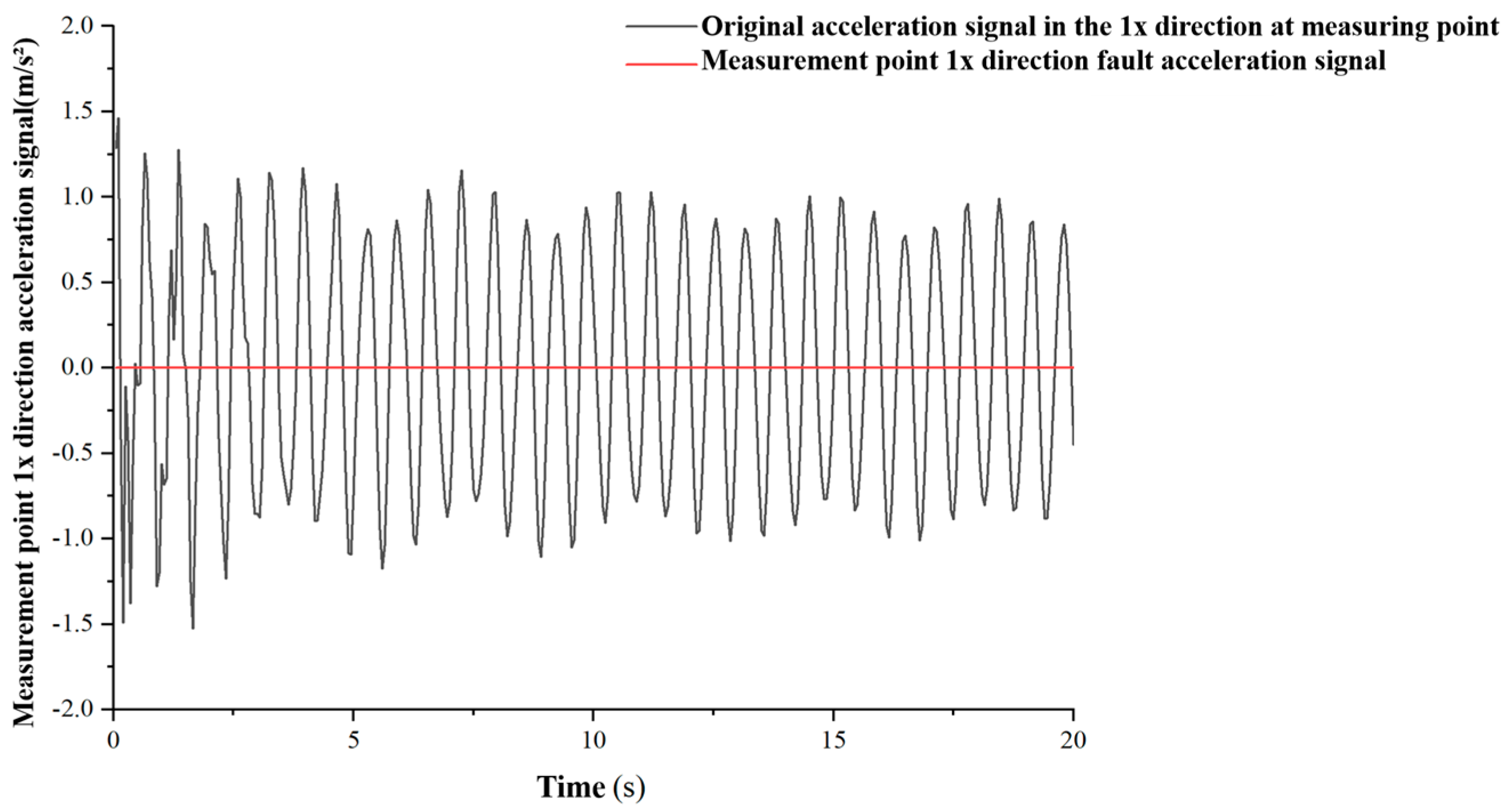
The following Figure 8 shows the comparison between the stuck fault signal generated based on the sensor fault mathematical model and the original normal signal of the acceleration signal in the 1x direction of the measuring point.
Figure 8.
Comparison between stuck fault signal and original normal signal.
2.1.3. Theory of Typhoon-Wave-Current Environmental Loads
The main structure of the platform is made of Q345 steel, with a density of 7850 kg/m3, an elastic modulus of 2.0 × 10¹¹ Pa, a Poisson’s ratio of 0.3, and a yield strength of 345 MPa. The total equivalent mass of the production equipment and living facilities on the upper deck is 4000 t, which is applied to the deck surface as a uniformly distributed surface load. The tubular members of the jacket are discretized using B31 beam elements, and the deck plate structure is modeled using shell elements. There are two classical approaches to simulating fluctuating wind fields, namely the linear filtering method and harmonic superposition method [31,32,33,34]. The harmonic superposition method requires a large number of trigonometric operations and has high computational overhead. The linear filtering method transforms Gaussian white noise into a stochastic process satisfying the target spectrum through recursive transformation, and features low memory usage and high computational efficiency, making it suitable for generating large batches of long-duration samples.
Typhoon wind fields are not strictly stationary stochastic processes, but have significant non-stationary characteristics. In recent years, scholars have conducted systematic research on these characteristics. However, from an practical engineering perspective, structural wind resistance design usually only selects wind speed samples within a short time window and focuses on the high-frequency components of pulsating wind. Therefore, this article adopts the theory of stationary stochastic processes to simulate the fluctuating wind duration of typhoons. Pulsating wind is essentially a three-dimensional random wind load induced by atmospheric turbulence, but considering the small impact of vertical and lateral turbulence on structural wind response, only the downwind fluctuating wind speed component is usually retained in engineering applications. Based on statistical analysis of a large number of measured samples, after excluding time-varying average wind speed, the downwind fluctuating wind speed can be approximated as a stationary Gaussian stochastic process with a mean of zero. The power spectral density function is a core parameter that characterizes the turbulent characteristics of fluctuating winds. It reflects the distribution of turbulent energy in the frequency domain, especially considering the particularity of typhoon wind fields. In response to the particularity of typhoon wind fields, this article adopts the empirical equation for the typhoon horizontal wind speed spectrum proposed by scholars such as Shi Yuan [35].
where , n the frequency of pulsating wind, the average wind speed at a standard height of 10 m, k ground roughness coefficient, and Sv(n) represents the power spectrum of pulsating wind speed at a height of 10 m.
Currently, numerical simulation research on pulsating wind fields mainly relies on two classic methods, namely linear filtering and harmonic superposition. The core mechanism of the linear filtering method lies in designing specific filters to transform the zero-mean Gaussian white noise sequence into a random process that conforms to the target spectral characteristics [36,37]. Its recursive equation is concise and clear, and the computational efficiency is significant. The harmonic superposition rule is based on the theory of trigonometric series, which regards fluctuating wind speed as a linear superposition of a series of harmonic waves with different frequencies, phases, and amplitudes, requiring a large number of trigonometric function operations and relatively high computational costs. Compared with the harmonic superposition rule, the linear filtering method has shown stronger applicability in the analysis of wind-induced responses of large-scale engineering structures due to its high computational efficiency, low memory consumption, easy programming implementation in recursive form, and obvious advantages in long-term wind field simulation [38]. Considering that this method can significantly reduce computational resource consumption while ensuring the reliability of simulation results, it is particularly suitable for engineering scenarios that require generating a large number of wind field samples or conducting long-term time history analysis. In this paper, the linear filtering method is selected as the core algorithm for generating fluctuating wind-speed time history to meet the dual requirements of wind load input efficiency and accuracy in subsequent analysis.
2.1.4. TCN Branch
TCN is a convolutional neural network architecture optimized for processing time-series data [39,40]. Its core innovation lies in the time convolutional layer, which systematically captures local patterns and long-range dependencies in a sequence by sliding multi-channel convolutional kernels in the time dimension, while avoiding the gradient vanishing problem and sequential dependencies in traditional RNNs [41]. TCN mainly consists of three important components.
(1) Causal convolution
Causal convolution, as the core mechanism of time-series modeling, essentially relies on temporal causality constraints to ensure that the output of the model at each time step depends only on the input data of the current and historical time points, completely excluding the potential influence of future time-point data. The mathematical expression for this temporal causal relationship is detailed in the following equation.
In the equation, yt represents the output value of time step t, K represents the length of the convolution kernel, wτ represents the weight coefficients of the convolutional kernel, and the input data xt−τ represent a time step of t − τ.
This design ensures that the model strictly follows temporal causality during the prediction process, yt outputs data that cannot be accessed to future times xt+1, xt+2, …, xt+n, avoids logical errors, and guarantees the reliability of temporal predictions.
At the implementation level, causal convolution ensures that convolution operations can only access current and previous data points on the timeline by precisely controlling the sliding direction and filling strategy of the convolution kernel. For example, when the convolution kernel slides along the timeline, its action area is always located on the left side of the current time step, avoiding any future data participation, thus naturally forming a one-way time flow constraint in the calculation process. The causal convolution diagram is shown below (Figure 9).
Figure 9.
Schematic diagram of causal convolution.
(2) Dilated convolution
Because efficient capture of long-range dependencies is required in time-series analysis, dilated convolution is introduced. Traditional standard convolution is limited by a fixed receptive field and requires stacking multiple layers or expanding the kernel size to expand the dependency range, but this can lead to a significant increase in computational complexity or information loss. Dilated convolution achieves sparse sampling of the input sequence through a dilation rate of d, with a d-value control on the sparsity of the sampling interval. In TCN, the expansion rate strictly follows the exponential rule, with the first layer d = 1 and subsequent layers d values doubling in sequence. Figure 10 is a schematic diagram of dilated convolution. This mechanism maintains the number of convolution kernel parameters unchanged and effectively expands the receptive field by inserting equidistant holes between the elements of the convolution kernel. The expression for dilated convolution is as follows.
Figure 10.
Schematic diagram of dilated convolution.
In the equation, x is a time series, d is the expansion rate, k represents the size of the convolution kernel, and s is the current time point.
(3) Residual connection
In TCN, the residual connection mechanism achieves efficient information transmission by directly adding the input features to the output of the convolutional layer, avoiding the exponential decay problem of gradients in deep networks. This design enables gradients to be directly fed back to shallow networks, improving training stability while allowing the network to build deeper architectures with fewer parameters, thereby capturing long-range temporal dependencies in shallow network structures.
2.1.5. GRU Branch
GRU, as a variant of RNN, effectively solves the inherent defect of traditional RNN in capturing long-term dependencies when processing long sequence data [42,43]. Compared to Long Short-Term Memory (LSTM) networks, GRU exhibits better training stability and convergence speed in handling long-sequence time-dependent tasks by reducing the number of parameters and optimizing the information flow path [44].
The GRU model only includes two gating structures, a reset gate and an update gate. The reset gate calculates candidate hidden states based on the current input and the hidden state of the previous time step, thereby suppressing the interference of irrelevant historical information, enabling the model to focus on key features of the current input and capture long-term time-series dependencies. The update gate is used to control the weight ratio of the previous state information in the current state, determine the degree of preservation of historical information, determine the final hidden state, and complete the output of the current time step. The working principle diagram of GRU is as follows (Figure 11).
Figure 11.
GRU working principle diagram.
The reset door expression is as follows.
rt = σ(Wr·[ht−1, xt])
In the equation, ht−1 represents the hidden state of the previous time step, input xt represents the current time step, Wr o resets the weight matrix connecting the hidden state ht−1 of the previous time and the input xt of the current time in the gate, and σ indicates the Sigmoid activation function.
The updated door expression is as follows.
zt = σ(Wz·[ht−1, xt])
In the equation, Wz represents the weight matrix connecting ht−1 and xt in the update gate.
The candidate hidden state expression is as follows.
In the equation, Wh and Uh represent the weight matrix corresponding to the memory unit, ⨀ represents element-level multiplication, and tanh represents the hyperbolic tangent activation function.
The final hidden state expression is as follows.
In the equation, I represents a vector of all 1s that is consistent with the zt dimensions.
2.2. Numerical Model Establishment
2.2.1. Establishment of Finite Element Model for Offshore Platform
In this study, a three-dimensional numerical solid model of the pipe-rack platform was independently constructed by the authors in ABAQUS software (2025). The model refers to the structural form of a real-world pipe-rack platform deployed in the South China Sea. Relevant design documents are internal research materials and have not been publicly released, so no published reference can be provided. No external entity or collaborative organization was involved in model establishment. In the finite element analysis modeling process, the boundary conditions and load distribution of the platform were reasonably set based on its actual working state. The bottom of the pile leg was simplified as a fixed support end due to its deep penetration into the seabed and being constrained by the soil to simulate the actual constraint situation. The model takes into account both the weight of the structure itself and the load-bearing capacity of the deck in the calculation. Among them, the weight of the upper production equipment, living facilities, etc. in the deck area is approximately 4000 tons after comprehensive conversion. This part of the load is uniformly distributed on the surface of the deck structure in the model. The model of the established pipeline rack platform is shown in Figure 12.
Figure 12.
Finite Element Model of Offshore Platform with Pipe Rack. (The finite-element model is independently built by the authors in ABAQUS. It refers to the structural layout of a real-world pipe-rack platform in the South China Sea, while relevant design documents are internal research materials and not publicly released).
2.2.2. Design of Typhoon Load Conditions
The water depth in the sea area where the prototype platform operates is 45 m. The ocean current shows a profile distribution that varies with water depth, with a surface velocity of 1.92 m/s, a mid-depth velocity of 1.42 m/s, and a bottom velocity of 1.12 m/s. Therefore, this paper adopts the linear filtering (autoregressive, AR) algorithm to simulate fluctuating typhoon wind speeds [45,46,47]. Ocean waves are characterized using the Donelan-modified JONSWAP spectrum to represent typhoon sea states. This spectrum adjusts the high-frequency decay exponent to −4, making it more consistent with measured characteristics of typhoon waves. The significant wave height and spectral peak period of the ocean waves are determined from the 10 m height mean wind speed through the dimensionless peak frequency equation. The three types of environmental loads—wind, waves, and currents—are synchronously coupled and applied in the ABAQUS transient dynamic solution, and the wind load time histories are applied to the platform members above the water surface according to height distribution. The combined loads of waves and currents are uniformly calculated through the Morison equation and applied to the submerged jacket members, and all wind, wave, and current loads use a completely unified transient analysis time step, achieving fully coupled dynamic response calculation of the jacket platform under wind, waves, and currents [48,49,50]. Figure 13, Figure 14, Figure 15, Figure 16, Figure 17, Figure 18, Figure 19 and Figure 20 are calculated using the algorithms and equations and plotted with Python 2025. This article designs typhoon loads at heights of 8 m,11 m, and 15 m. The time history of fluctuating wind speed at 8 m is as follows.
Figure 13.
Time history of fluctuating wind speed at 8 m.
The time history of fluctuating wind speed at 11 m is as follows.
Figure 14.
Time history of fluctuating wind speed at 11 m.
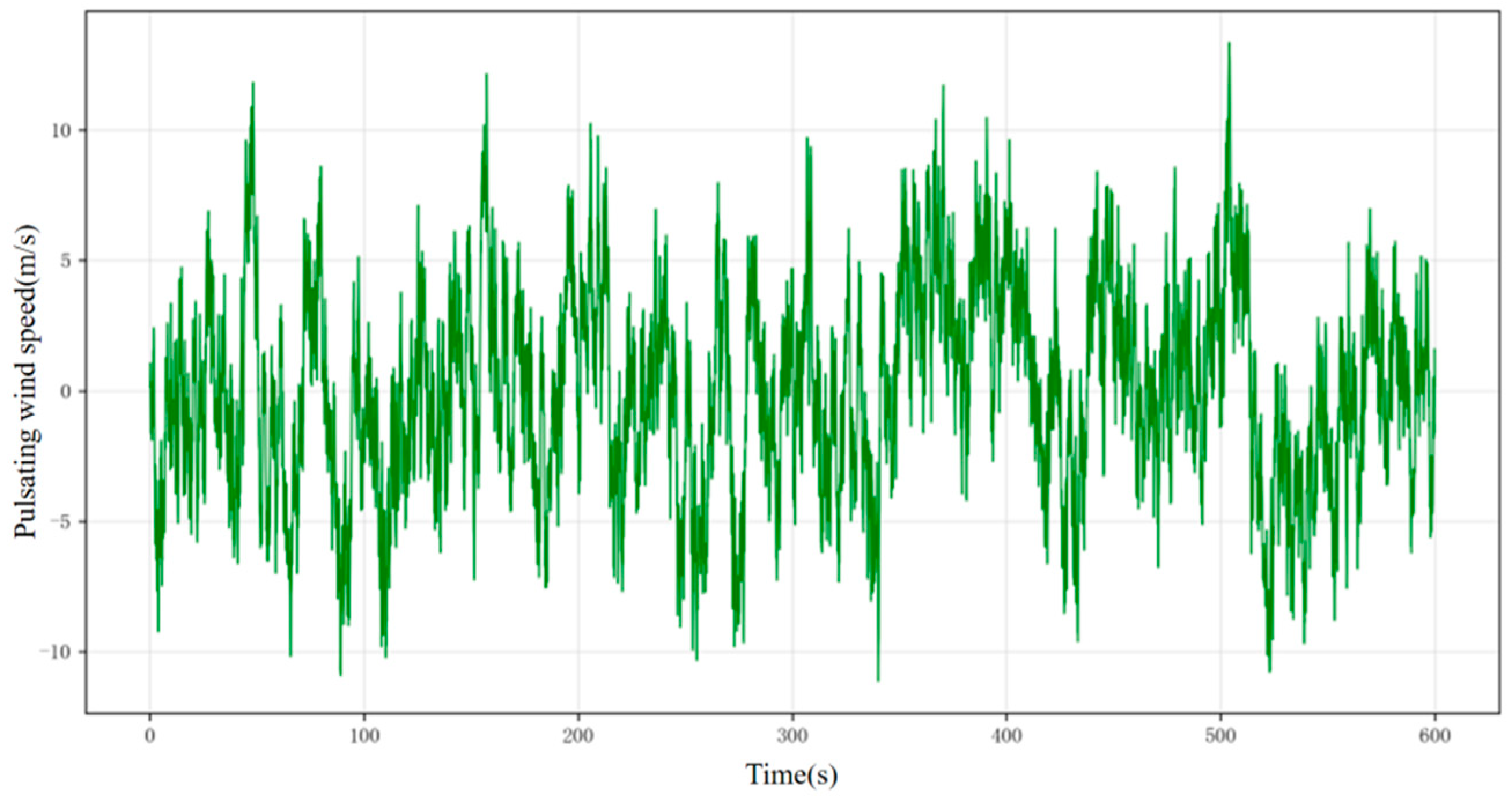
The time history of fluctuating wind speed at 15 m is as follows.
Figure 15.
Time history of fluctuating wind speed at 15 m.
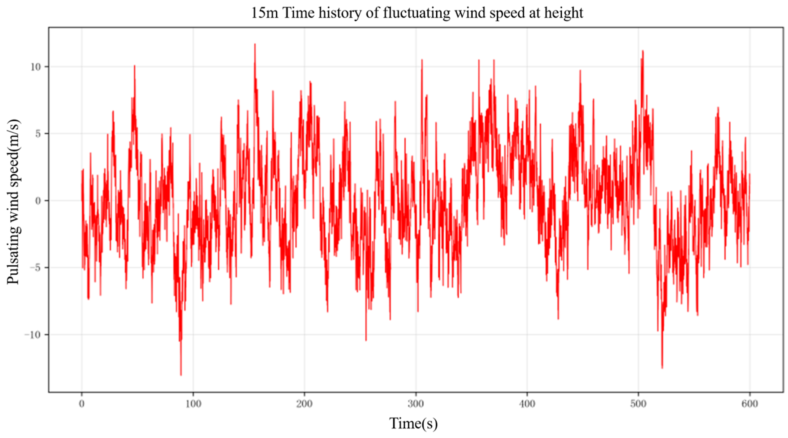
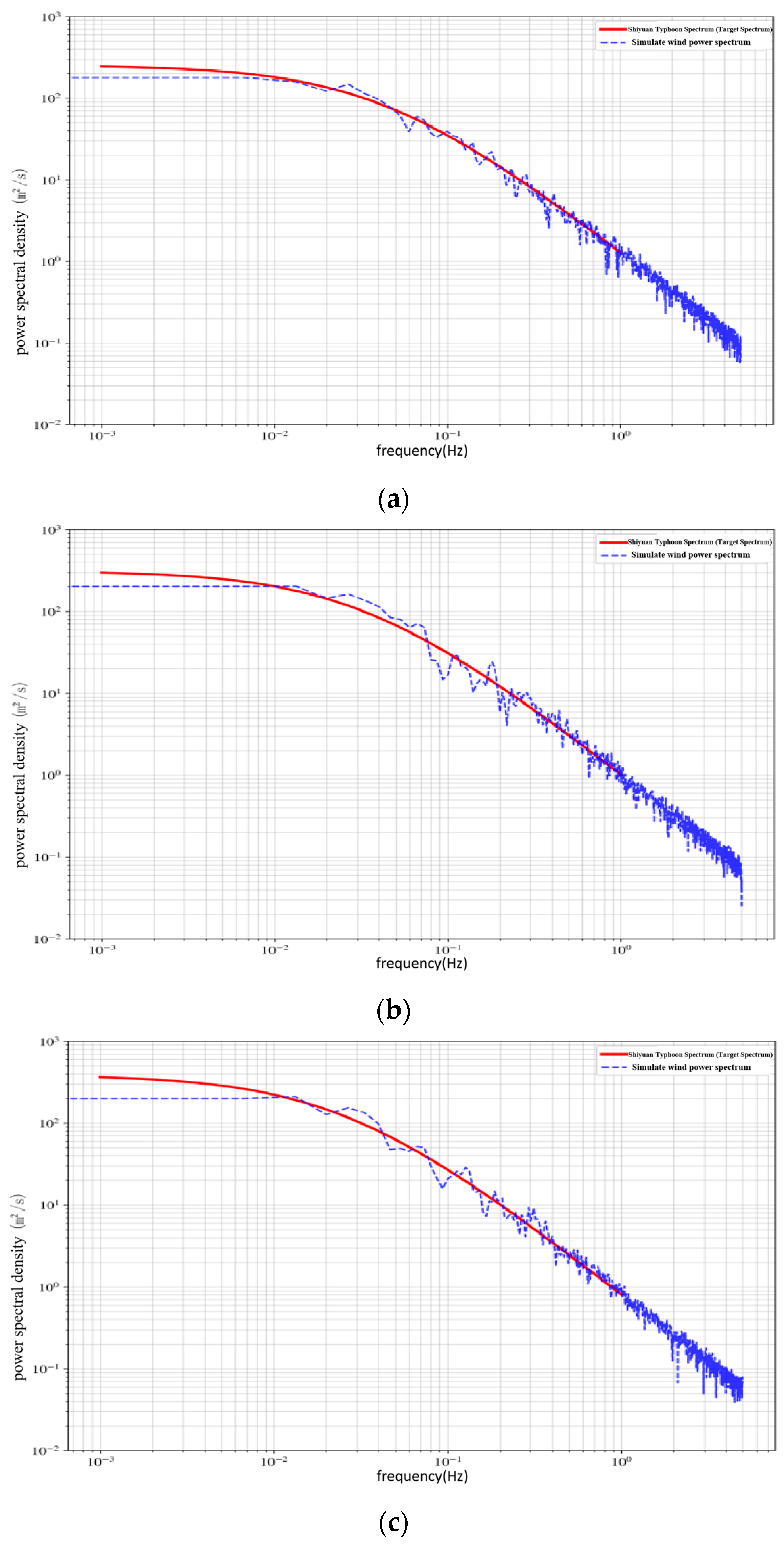
To verify the effectiveness and accuracy of numerical simulation of pulsating wind fields, this study conducted power spectral density analysis on the generated pulsating wind speed time history samples, and systematically compared and verified the simulated wind spectrum with the empirical equation of the Shiyuan typhoon spectrum. The following Figure 16 shows the results of comparison between the simulated wind power spectral density curves at heights of 8 m, 11 m, and 15 m and the target spectral curve of Typhoon Shiyuan. It can be clearly observed from the Figure 17 that the simulated wind spectrum shows good consistency with the target curve of the Shiyuan typhoon spectrum in terms of the overall variation trend, indicating that the pulsating wind time history samples generated by the linear filtering method in this paper can effectively capture the dominant frequency components and turbulent energy distribution characteristics of the typhoon wind field. In the high-frequency range, the simulated wind spectrum exhibits random fluctuations around the target spectrum curve, but remains highly consistent with the target spectrum. In summary, the simulated wind power spectrum can accurately reflect the turbulent energy distribution law described by the Shiyuan typhoon spectrum in the frequency domain characteristics, verifying the rationality and reliability of the numerical simulation model of the downwind pulsating wind field in this paper. It can provide wind load input conditions that are in line with the actual characteristics of the typhoon wind field for the subsequent analysis of the dynamic response of the pipe-rack offshore platform under the typhoon.
Figure 16.
Comparison between simulated spectrum and target spectrum. (a) Comparison of simulated spectrum and target spectrum at 8 m. (b) Comparison of simulated spectrum and target spectrum at 11 m. (c) Comparison between simulated spectrum and target spectrum at 15 m.
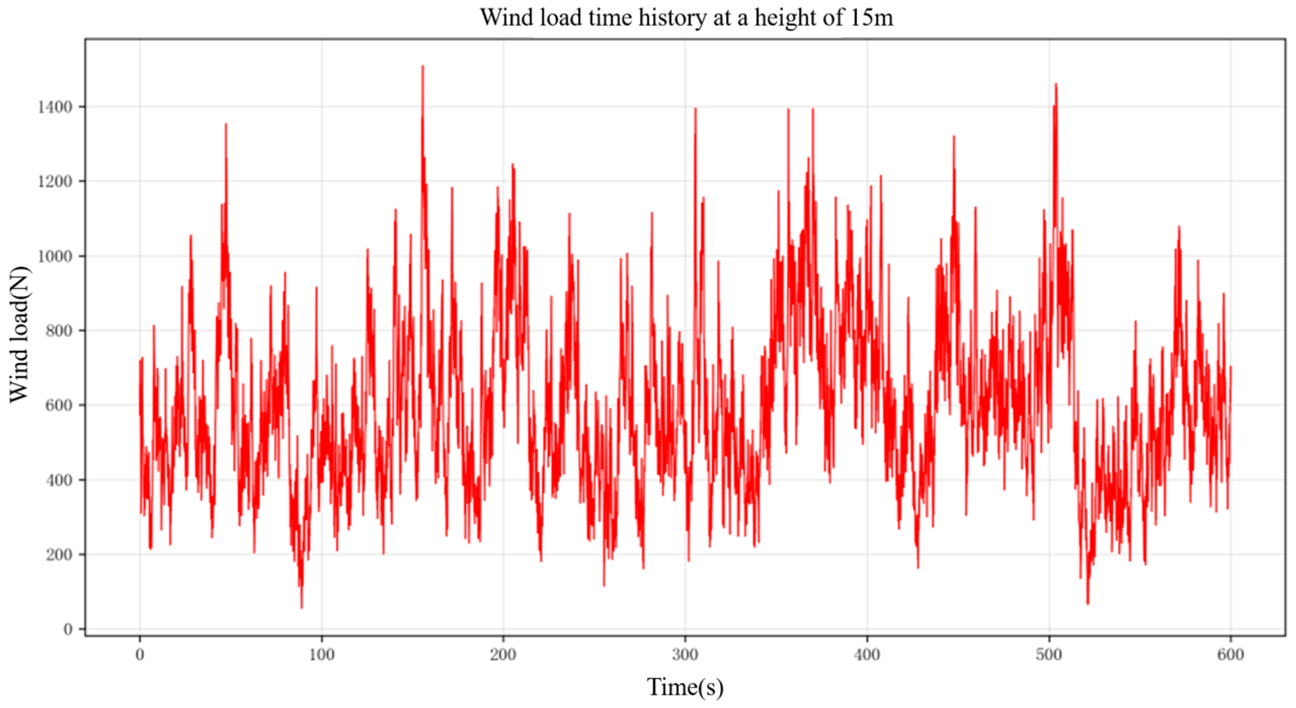
According to the equation A, calculate the wind load time history at 8 m, 11 m, and 15 m, as shown in the following Figure.
Figure 17.
Time history of wind load at 8 m.
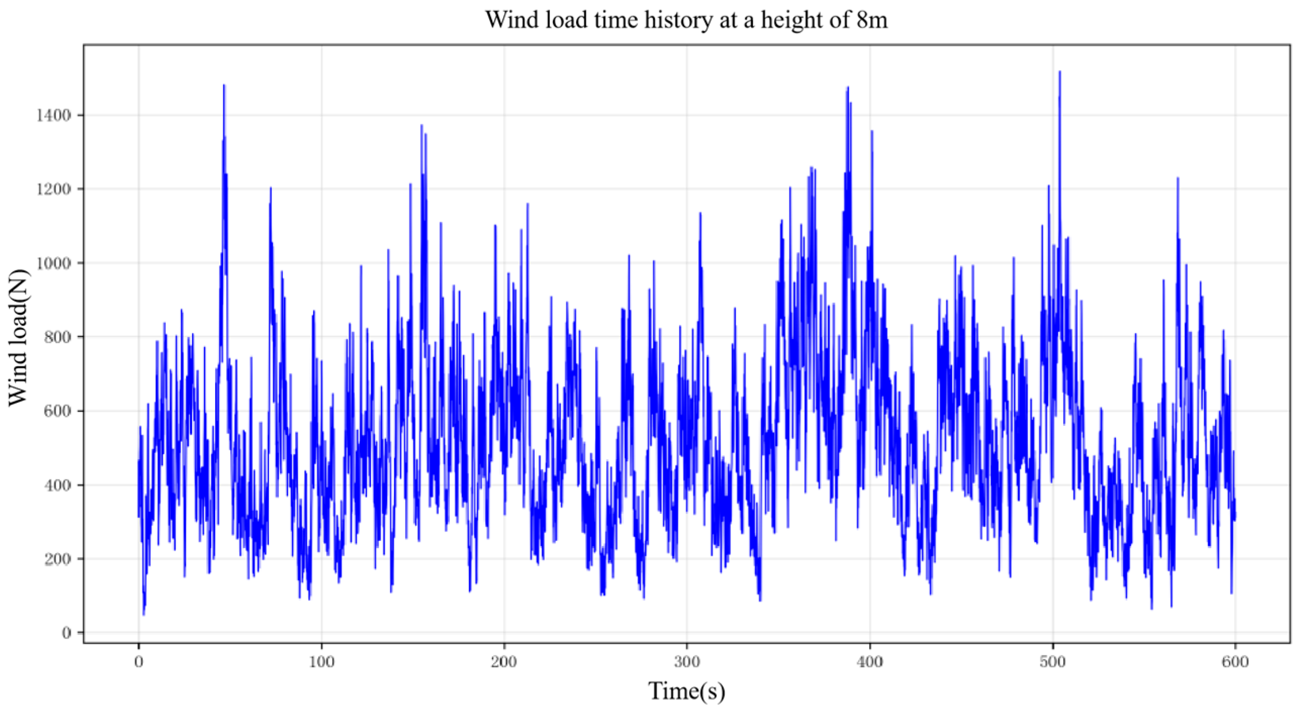
Figure 18.
Time history of wind load at 11 m.
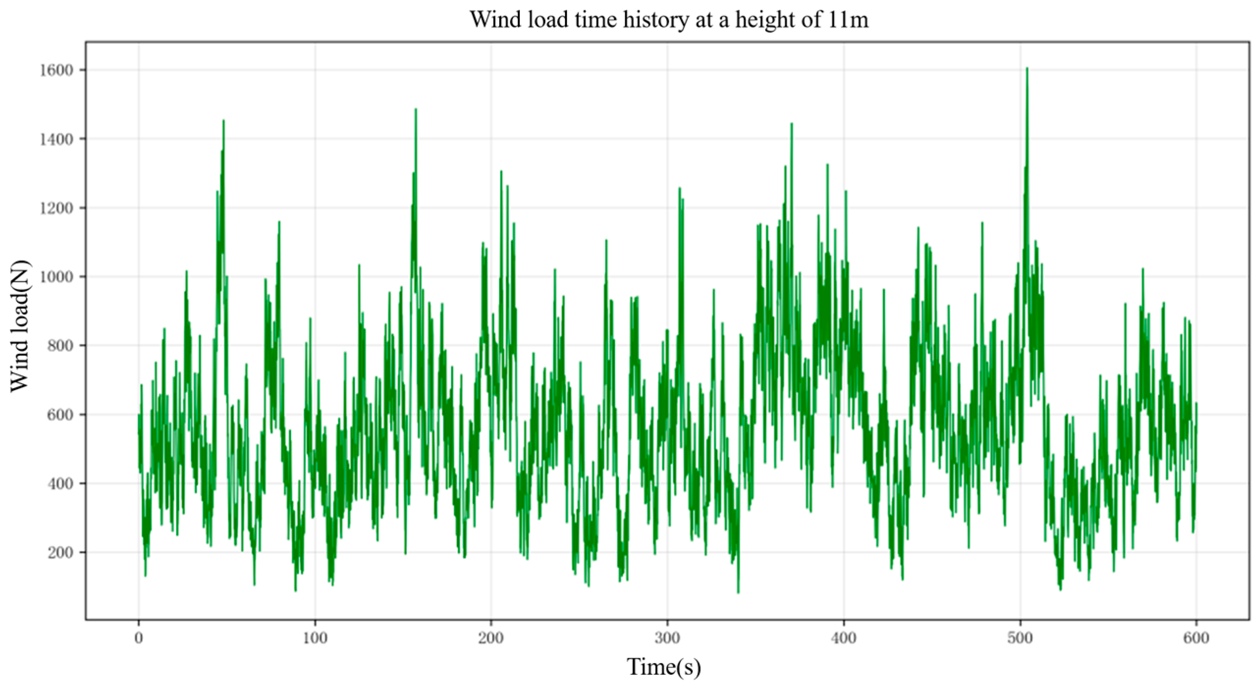
Figure 19.
Time history of wind load at 15 m.
According to the equation and the current ocean environment, set the ocean current velocity (Table 3) as follows.
Table 3.
Current velocities at different locations.
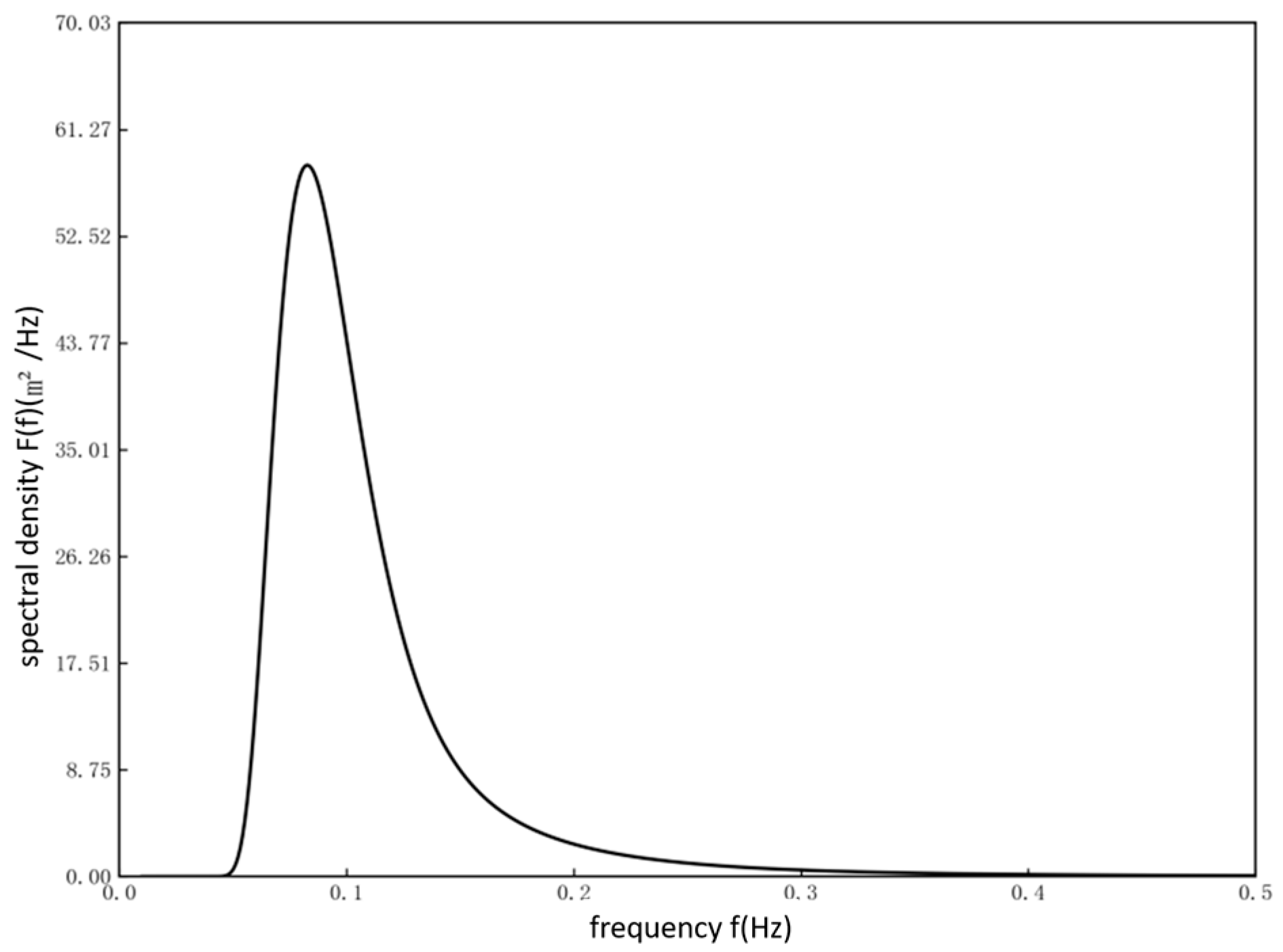
The JONSWAP spectrum, as a widely used standard wave-spectrum model in the international ocean engineering field, can accurately describe the spectral characteristics of waves under typhoon conditions. Its spectral function has good applicability in characterizing the energy distribution law, peak frequency position, and high-frequency attenuation characteristics of typhoon waves. This article uses Donelan’s improved JONSWAP spectral form to describe the spectral characteristics of waves under typhoon conditions [51]. The main improvement of this spectral form compared to the standard JONSWAP spectrum is that the high-frequency attenuation index is adjusted f−5 from to f−4, which is more in line with the measured data and theoretical basis of typhoon waves. It can effectively characterize the distribution law of wave energy in the frequency domain under typhoon sea conditions.
In the equation, F(f) is the frequency spectral density, f is wave frequency, fp is spectral peak frequency, g is acceleration due to gravity, β is a spectral scale parameter, γd is the spectral peak enhancement factor, and σ is the spectral width parameter.
The spectral parameters are determined by dimensionless peak frequency using the following equation.
In the equation, v is the average wind speed at a height of 10 m.
The following Figure 20 shows the improved JONSWAP spectrum based on Donelan.
Figure 20.
Improved JONSWAP spectrum based on Donelan.
2.3. Proposed Methodology and Implementation
2.3.1. Data Preprocessing
(1) Sliding window
The segmentation of fault acceleration signals adopts a sliding window strategy based on temporal continuity, with a window length of 100. This ensures the temporal integrity of the damage evolution process while avoiding the increase in computational complexity caused by excessively long sequences. The window length, sliding step, overlap rate and 6:2:2 dataset-split ratio are experimental settings determined for the present study. The sliding step is set to 50, forming a 50% overlap rate, so that adjacent sequences contain sufficient temporal correlation information and the model can capture the continuous dynamic characteristics of damage evolution [52,53].
To avoid information leakage caused by overlapping windows, the data split in this paper was performed by complete simulation runs before windowing and augmentation. Each simulation run corresponds to one complete finite element simulation time history under a given fault condition and a given random seed. The runs were first divided into training, validation, and test sets at a ratio of 6:2:2, with no run shared across subsets. Subsequently, sliding-window segmentation is performed for all three subsets, while time-domain augmentation is only applied to the training set rather than validation and test sets. As a result, overlapping windows generated from the same run always remain in the same subset, and the test set consists entirely of simulation runs that were not involved in training (Figure 21).
Figure 21.
Schematic diagram of sliding window.
(2) Time-domain enhancement
To improve the generalization ability of the model, time-domain augmentation is only implemented for training samples. A random offset of ±10% of the sequence length is added to each training sequence to simulate small differences in the onset time of damage. No time-domain augmentation is conducted for the validation set and test set, which keep the original raw time-series signals for unbiased performance evaluation (Figure 22).
Figure 22.
Schematic diagram of time-domain enhancement.
2.3.2. Parallel Fusion Architecture
To achieve high-precision intelligent diagnosis of sensor faults, this paper constructs a deep neural network model that integrates TCNs and convolutional gated recurrent units. The entire diagnostic process covers core steps such as data collection and preprocessing, dataset partitioning, model construction, training optimization, and optimal model preservation. The specific description is as follows.
First, obtain the original sensor acceleration signal. Based on different damage modes, corresponding fault acceleration signals are constructed through Section 2.2 of this article to form a raw sample library containing multiple types of faults. Subsequently, the sliding window technique was used to segment the continuous temporal signals and normalize them, ultimately constructing a standard dataset. Divide the constructed sample set into a training set, a validation set, and a testing set according to a predetermined ratio. The training set is used to drive model parameter updates, the validation set is used to monitor the generalization ability during the training process and guide early stopping strategies, and the test set is used for independent performance evaluation of the final model.
During the model construction phase, design a TCN-GRU fusion neural network. The input layer receives preprocessed acceleration data, which include acceleration responses of 7 measurement points in the X, Y, and Z directions. Parallel feature extraction will input both TCN and GRU branches simultaneously. The TCN branch is composed of multiple causal convolution blocks stacked together, each block containing causal convolution, batch normalization, ReLU activation, and Dropout. It uses dilated convolution and residual connections to expand the receptive field and accelerate training, outputting high-level features with long-range temporal dependencies. The GRU branch adopts multi-layer units, each of which achieves local temporal dynamic modeling through reset gates and update gates. The hidden state is iteratively transmitted along time steps, and the local feature sequence of each time step is output. The output of the two branches is concatenated along the feature dimension and compressed into a fixed length feature vector through adaptive global average pooling. It is then sent to a fully connected layer, where ReLU activation and Dropout regularization are applied after each layer, gradually mapping to the category space. Finally, Softmax outputs the probabilities of each category to achieve intelligent diagnosis of sensor faults.
The intelligent diagnosis process for sensor faults based on the TCN-GRU neural network is as follows (Figure 23).
Figure 23.
TCN-GRU neural network fusion diagram.
(1) Dual-branch feature extraction
The TCN branch utilizes dilated convolution to efficiently capture long-range temporal dependencies in shallow networks, while ensuring stable gradient propagation through residual connections to extract high-level representations containing global patterns and periodic features. The GRU branch dynamically processes local dynamic changes in the sequence through an adaptive gating mechanism of reset and update gates. Reset the gate to suppress interference from irrelevant information and update the fusion ratio between the gate control historical state and new features, so that the model can filter noise and extract temporal evolution features of the sequence, achieving modeling of short-term dynamic relationships.
(2) Feature fusion
The output features of the two branches are concatenated and fused in the feature dimension to ensure that the long-range dependent features captured by TCN and the sequence dynamic features extracted by GRU complement each other while maintaining their respective feature space independence. This fusion method avoids the loss of feature information caused by serial transmission and retains the core advantages of both models.
(3) Feature compression and task output
The fused feature sequence is compressed into a fixed dimensional vector representation through global average pooling operation, which preserves temporal statistical characteristics and eliminates temporal redundancy. Finally, the compressed feature is mapped to the target space through a multi-layer fully connected classifier to complete the classification prediction task.
2.3.3. Training Configuration
For the convenience of training and hyperparameter adjustment of neural networks, the computer system used in this study was equipped with the Windows 11 Professional Edition, an NVIDIA GeForce RTX 4070 graphics card (NVIDIA Corporation, Santa Clara, CA, USA), a 13th Gen Intel (R) Core (TM) i5-13600KF processor (Intel Corporation, Santa Clara, CA, USA) running at 3.50 GHz, and 64.0 GB of running memory. The Python version used is 3.12.2. The neural network is trained on the Pycharm platform, with Pycharm version 2024.2.3. All five repeated experiments adopt exactly the same dataset partitioning scheme, network architecture, hyperparameters, and data preprocessing pipeline. The partitioning of the numerical simulation dataset and the scaled-model physical experimental dataset remains fixed across all five experiments. The randomness originates only from network weight initialization and Dropout during the training phase. In each run, the accuracy, precision, recall, and F1 score on the test set are recorded. Within a single experiment, a global random seed is set to fix the random state of the data preprocessing stage. The weight-initialization seed is not fixed across the five experiments, thereby reproducing the genuine natural random fluctuation of model training. Dropout is enabled only during training and disabled during inference. All experiments use a unified early-stopping rule. The validation-set loss is monitored, and if the validation loss does not decrease for 50 consecutive epochs, training is stopped and the best model is saved. The statistical results of five repeated experiments on the numerical simulation dataset showed an accuracy of 97.21 ± 0.28%, precision of 96.83 ± 0.31%, recall of 96.54 ± 0.35%, and F1 score of 96.62 ± 0.30%. The statistical results of five repeated experiments conducted on the scaled model physics experimental dataset showed an accuracy of 91.06 ± 0.24%, precision of 91.14 ± 0.27%, recall of 90.99 ± 0.30%, and F1 score of 90.92 ± 0.26%. The specific information based on the TCN-GRU neural network architecture is shown in Table 4. The training parameter settings based on the TCN-GRU neural network are detailed in Table 5.
Table 4.
Neural Network Architecture and Training Configuration Based on TCN-GRU Neural Network.
Table 5.
Training Parameter Settings Based on TCN-GRU Neural Network.
3. Results
3.1. Numerical Simulation Experiment
3.1.1. Experimental Setup
This study systematically analyzed the training process of the TCN-GRU sensor fault intelligent diagnosis model, and the model loss curve is shown in the following Figure 24.
Figure 24.
Loss curve based on TCN-GRU sensor fault intelligent diagnosis model.
From the loss curve, both the training loss and validation loss decrease rapidly in the early stages of training, indicating that the model quickly converges from the random initialization state to the optimal parameter region. After about 20 cycles, the loss decrease tended to flatten out, and the two curves remained closely aligned without any significant deviation, indicating that the model did not overfit and had good generalization ability. Based on the above curve characteristics, it can be concluded that the proposed TCN-GRU fusion model has a smooth training process, rapid convergence, and exhibits high accuracy and strong robustness on the validation set.
This study systematically evaluates the classification performance of the TCN-GRU sensor fault intelligent diagnosis model based on a confusion matrix. The confusion matrix is shown in the following Figure 25.
Figure 25.
Confusion matrix based on TCN-GRU sensor fault intelligent diagnosis model.
The results indicate that the damage diagnosis model based on TCN-GRU has excellent ability to distinguish damage types. According to the confusion matrix analysis, Damage 5 achieves the highest recall of 99.80%, followed by Damage 3 (99.49%) and Damage 9 (99.35%). The recall of Damage 10 is 97.60%, Damage 1 is 98.72%, Damage 7 is 96.30%, Damage 4 is 96.05%, Damage 2 is 95.90%, Damage 6 is 95.60%, and Damage 8 is 94.70%. The overall accuracy of the model reached 97.34%. This high-precision classification capability effectively solves the problem of category confusion caused by feature similarity in sensor fault diagnosis, enabling the model to provide stable and accurate sensor fault diagnosis results, meeting the basic requirements for diagnostic reliability in practical engineering applications.
To visually evaluate the intrinsic representation ability of the TCN-GRU model for sensor fault features, the t-distribution random neighborhood embedding algorithm was used to perform dimensionality reduction and visualization analysis on the high-dimensional features of the test-set samples before and after model training. Figure 26 shows the distribution of raw acceleration data directly mapped to two-dimensional space after preprocessing. The sample points of different fault types in the Figure are interwoven, and the boundaries are blurred, without forming any obvious clustering structure. The samples of various types are highly mixed in the feature space, indicating that it is difficult for the original high-dimensional features to effectively distinguish different damage modes. Figure 26 represents the distribution pattern after training. The originally discrete and disordered sample points gradually converge into several independent clusters with clear boundaries and strong cohesion. The inter-cluster distance corresponding to each fault category increases significantly, and the intra-class samples are tightly clustered, showing good feature separability. This change demonstrates the hierarchical abstraction process of the original multi-channel acceleration signal by the TCN-GRU model through multi-layer cascaded temporal convolution and gated loop units. The low-level network captures local transient responses, whereas the high-level network gradually integrates temporal context and strengthens fault-sensitive features and finally forms feature representations with strong discriminative ability in the high-dimensional embedding space. The t-SNE visualization results verify that the proposed model can effectively write complex response laws under different damage modes from the perspective of feature learning, map the original hybrid data into separable feature structures, and capture separable features strongly related to fault types from the high-dimensional feature space to achieve accurate identification of different sensor faults.
Figure 26.
(a) t-SNE graph before training; (b) t-SNE graph after training.
According to the accuracy, precision, recall, and F1 scoring equations, various evaluation indicators for constructing the TCN-GRU sensor-fault intelligent diagnosis model are detailed in Table 6.
Table 6.
Accuracy, Precision, Recall, and F1 Value of TCN-GRU Sensor-Fault Intelligent Diagnosis Model.
3.1.2. Working Conditions
To conduct research on the intelligent diagnosis model of sensor faults based on TCN-GRU, this paper systematically constructs a multidimensional sensor-fault condition library and generates standardized fault datasets by controlling fault parameters. The specific sensor fault settings and corresponding fault category labels for each experimental condition are shown in the table (Table 7) below.
Table 7.
Sensor Fault Settings and Corresponding Labels.
3.1.3. Dataset for Numerical Simulation
The acceleration sensor signals under different working conditions were extracted through the experimental scheme of this article. The following Figure 27, Figure 28 and Figure 29 show the acceleration signals in the xyz directions collected from measuring point 1 of the offshore platform of the pipeline rack in a healthy state.
Figure 27.
Acceleration signal in the 1x direction at measuring point.
Figure 28.
Acceleration signal in the 1y direction at measuring point.
Figure 29.
Acceleration signal in the 1z direction at measuring point.
Based on the sensor-fault mathematical model in Section 2.1.1 of this article, the acceleration signal is modeled, and then the dataset is subjected to sliding-window and time-domain enhancement in Section 2.1.5.
3.1.4. Experimental Results and Analysis
Based on the equations for accuracy, precision, recall, and F1 score, construct a table (Table 8) of various evaluation indicators for the TCN-GRU sensor-fault intelligent diagnosis model. It should be noted that the above-mentioned diagnostic accuracy derives from synthetic faults mathematically superimposed on healthy measured signals of the laboratory-scale test model, instead of natural sensor-failure faults.
Table 8.
Diagnostic Results of the TCN-GRU Model on the Scaled Experimental Sensor Composite Fault Dataset.
3.1.5. Comparative Experiment
To verify the performance of the TCN-GRU sensor-fault intelligent diagnosis model proposed in this article, this section (Figure 30) will compare it with TCN alone and GRU alone. The following is a table (Table 9) and comparison chart of the accuracy, precision, recall, and F1 value of three sensor fault diagnosis methods.
Figure 30.
Comparison of accuracy, precision, recall, and F1 value of four sensor-fault diagnosis methods.
Table 9.
The Accuracy, Precision, Recall, and F1 Score of Four Sensor Fault Diagnosis Methods.
From the data in the above Figure, we can see that the TCN-GRU fusion model is significantly better than the single model in four evaluation indicators, with an overall accuracy rate of 97.34%, average accuracy rate of 96.94%, average recall rate of 96.67%, and F1 value of 96.73%. The accuracy of the standalone TCN model is 89.2%, with an F1 value of 90.90%. The accuracy of the GRU model alone is 84.8%, with an F1 score of 86.90%. The TCN-GRU fusion model organically combines the advantages of both, i.e., the TCN branch is responsible for capturing the global temporal evolution law, the GRU branch focuses on local detail changes, and the outputs of the two branches are input into the classifier after feature fusion and global average pooling, achieving complementary and enhanced multi-scale temporal features. In the task of identifying damage to a pipe-rack offshore platform structure, the comparative results fully verify the superiority of the proposed fusion architecture, which can fully mine fault-sensitive information from multi-channel acceleration responses and improve diagnostic accuracy and reliability.
To further verify the advantages of the parallel fusion architecture, this study additionally constructs a TCN-GRU serial fusion baseline model with a comparable parameter scale. The processing pipeline of the serial model is as follows. The time-series signal is first fed into the TCN module to extract temporal features, and the feature sequence output by TCN is directly passed to the GRU module for further feature learning. This is followed by a global average pooling layer, a fully connected layer and a Softmax output layer identical to those in the parallel model. This serial baseline and the proposed parallel TCN-GRU model adopt exactly the same dataset partitioning strategy, sliding window, time-domain augmentation scheme and training hyperparameters to ensure fair comparison and eliminate the interference of differences in network parameter quantity with experimental results. As shown in Table 9 and Figure 30, the serial fusion model achieves better overall performance than the single TCN and single GRU models, yet all evaluation metrics are lower than those of the parallel TCN-GRU model proposed in this paper. The serially stacked architecture suffers from temporal information decay during the layer-by-layer propagation of features, which degrades the feature discrimination ability for compound faults with highly aliased features such as drift plus stuck faults. In contrast, the parallel architecture enables TCN and GRU to extract features independently before concatenation and fusion along the feature dimension. It preserves the respective feature subspaces of the two sub-networks and avoids information loss caused by serial propagation. This architecture achieves more sufficient fusion of long-term slowly evolving features and local transient abrupt features, making it more suitable for multi-sensor compound fault identification tasks on offshore platforms.
3.2. Scale-Model Physical Experiment of Offshore Platform
3.2.1. Experimental Equipment
Build an indoor pipeline rack ocean platform model and use a data acquisition system to extract data from the model. The data acquisition system mainly consists of sensors, force hammers, exciters, and signal acquisition systems.
(1) Pipeline rack offshore platform
The offshore platform (Figure 31) model of the pipeline rack is shown in the following Figure, with an overall height of 1.53 m and a total weight of approximately 60 kg. The model simulates the quick disassembly and working condition simulation of damaged components in different structural states through flange connections.
Figure 31.
Model of offshore platform with pipeline support.
(2) Sensor
The sensor system comprises a 1A312E (Figure 32) piezoelectric triaxial acceleration sensor, which includes three mutually perpendicular shear-structure cores and can synchronously output X, Y, and Z axis acceleration signals.
Figure 32.
1A312E Piezoelectric three-way acceleration sensor.
(3) Signal testing system
The DH5922D dynamic signal testing (Figure 33) and analysis system adopts a standard chassis structure, relies on Gigabit Ethernet for data communication, and expands test channels through switches. Only a single computer is needed to control multi-channel dynamic signal parallel synchronous testing and analysis.
Figure 33.
DH5922D signal testing system.
3.2.2. Test Condition Settings
To verify the research on the intelligent structural damage diagnosis model based on CNN ResNet and the sensor fault intelligent diagnosis model based on TCN-GRU proposed in this article, this experiment obtained acceleration signals through a data acquisition system by simulating the health status and local damage of the pipe-rack offshore platform.
The experimental model is placed in a sand bucket and fixed with four pile legs buried in sea sand to simulate the boundary conditions of the pipe-rack offshore platform in the seabed. The exciter is fixed on a platform model pile leg to apply random load excitation. The testing process collects acceleration signals through acceleration sensors under six preset structural conditions and one healthy condition on the pipe-rack offshore platform.
3.2.3. Physical-Experiment Dataset Construction
The acceleration sensor signals under different working conditions were extracted through the experimental scheme in Section 3.2.1 of this article. The following Figure 34, Figure 35 and Figure 36 show the acceleration signals in the xyz directions collected by measuring point 1 of the offshore platform of the pipeline rack under working condition 1.
Figure 34.
Measurement point 1X direction acceleration signal.
Figure 35.
Measurement point 1Y direction acceleration signal.
Figure 36.
Measurement point 1Z direction acceleration signal.
The two-dimensional RGB image obtained by TRMTF of the acceleration signal of measuring point 1 after sliding the window in operating condition 1 is shown below (Figure 37).
Figure 37.
Two-dimensional RGB acceleration signal obtained by TRMTF after sliding window of measurement point 1. (a) Measurement point 1 sliding window 1 2D RGB image. (b) Measurement point 1 sliding window 2 2D RGB image. (c) Measurement point 1 sliding window 3 2D RGB image.
3.2.4. Test Results and Analysis
To validate the intelligent structural damage diagnosis model based on CNN ResNet, sensor fault diagnosis was performed on the offshore platform of the pipeline rack according to the process outlined.
The damage diagnosis model loss curve of the jacket platform structure is shown in the following Figure 38.
Figure 38.
Loss curve based on CNN ResNet structural damage recognition model.
This study systematically evaluates the classification performance of the damage diagnosis model for the jacket platform structure through a confusion matrix. The confusion matrix is shown in the following Figure 39.
Figure 39.
Confusion matrix of the CNN ResNet model for structural damage diagnosis of the jacket platform.
The results indicate that the damage diagnosis model based on CNN-ResNet has excellent ability to distinguish damage types. The model has stable feature extraction and classification capabilities under complex working conditions. The damage diagnosis model based on CNN-ResNet exhibits strong robustness under extreme environmental conditions of typhoon wave combined action, effectively overcoming the noise interference and similar damage characteristics of multi-source sensor data, providing reliable technical support for real-time and accurate diagnosis of structural damage on offshore platforms. Its classification performance fully verifies the application value of the CNN-ResNet neural network architecture in the field of structural health monitoring.
According to the equations for accuracy, precision, recall, and F1 score, the various evaluation indicators based on the CNN ResNet structural damage recognition model are shown in the following Table 10.
Table 10.
Structural Sensor Fault Diagnosis results of the CNN-ResNet model.
Table 10 shows that the CNN-ResNet-based structural damage diagnosis model achieves an accuracy of 88.33% in the scaled-model physical experiment, indicating that the model can reliably identify the preset structural damage conditions of the pipeline rack platform.
4. Discussion
The TCN branch relies on causal convolution and multi-layer dilation convolution to fully capture the long-term temporal changes in sensor drift faults that slowly evolve over time, while the GRU relies on a dual-gate control structure with reset and update gates, which has higher recognition sensitivity to transient changes in gain faults and local dynamic signals of stuck-at faults. This study adopts a dual-branch parallel fusion architecture, in which the two networks extract features independently and then perform concatenation-based fusion. This architecture avoids temporal information loss induced by serial transmission and complements the advantages for both long-term gradual faults and instantaneous abrupt faults, effectively improving the discrimination capability for multiple types of composite faults.
Under composite-fault conditions, interference exists among multi-point and multi-type fault signals, leading to heavily overlapped fault features and increased identification difficulty. In working condition 8 of this paper, five sensors suffer from different simultaneous faults and produce highly overlapping sample features. Although the classification accuracy for this working condition drops to 98.75%, it still remains at a relatively high level. The overall dataset accuracy reaches 97.34%, which demonstrates that the proposed TCN-GRU fusion model achieves stable and reliable diagnostic performance for highly coupled composite faults within the scope of the numerical-simulation and laboratory-scale test datasets used in this work.
It should be emphasized that all fault samples in this work are mathematically synthesized faults artificially injected into measured healthy signals, rather than real-world fault recordings from naturally failed offshore sensors. Physical validation only takes place under laboratory conditions using a scaled-down platform model. For this reason, the reported model performance does not directly transfer to full-scale practical deployments in real offshore marine environments.
The sensor-fault mathematical model constructed in this paper adopts only constant and linear fault adjustment parameters and simulates merely five basic fault modes with fixed-amplitude or linear-variation characteristics. Complex real-world fault patterns such as intermittent jumps and nonlinear time-varying degradation are not considered, which creates a certain deviation from the actual degradation behaviors of marine sensors. Future work may embed a multi-head attention mechanism into the TCN-GRU dual-branch architecture to adaptively focus on fault-sensitive time segments, strengthen the extraction of weak and nonlinear fault features, and further boost model generalization under complex operating conditions.
It should be noted that the above-mentioned closed-set classification property determines that the model only outputs probability distributions for the 10 predefined composite-fault categories. It cannot judge whether an input sample belongs to an unknown category. When fed with healthy-sensor signals, single-fault samples or unseen new fault combinations outside the training library, the model will forcibly assign inputs to the category with maximum probability among the 10 known classes and consequently produce misdiagnosis. Accordingly, the applicability prerequisite of the present model is that test samples should belong to the 10 composite-fault modes covered during training. For practical open-environment application, an open-set recognition mechanism needs to be introduced, and the working-condition library should be expanded to include healthy states, single faults and more unseen composite-fault cases in follow-up research.
This paper chooses parallel fusion instead of serial stacking. Serial hybrid architectures tend to suffer from temporal information loss and single-sided feature representation in deep information propagation, yielding unsatisfactory robustness and classification accuracy, especially for offshore-platform-like scenarios with multi-measurement-point signals, heavy noise and heavily overlapping composite-fault features. By contrast, the parallel-fusion scheme enables TCN and GRU to perform feature extraction independently in their own feature spaces before feature concatenation. It maintains the independence of two feature sub-spaces and prevents information attenuation caused by serial transmission. From the perspective of the existing literature, analytical-model-driven methods are hard to accurately deploy for complex offshore structures. Signal-processing-based approaches depend on hand-crafted signal indicators and show limited generalization. Pure CNN models are constrained by local receptive fields and insufficient for long-range dependency capture. Vanilla RNN-variant models face low training efficiency and gradient-vanishing risks. Serial hybrid networks, despite combining merits from two branches, still suffer from temporal information loss. The proposed TCN-GRU parallel-fusion model targets these drawbacks, capturing both long-range temporal dependencies and local dynamic evolution features via parallel feature extraction and feature-level fusion, as validated on numerical-simulation data and laboratory-scale physical experimental data in this study.
5. Conclusions
This article proposes an intelligent sensor-fault diagnosis model based on the parallel fusion of TCN and GRU, aiming to tackle a technical challenge that existing time-series diagnostic models struggle to achieve, namely simultaneously capturing both long-range dependencies and local dynamic evolution features, for the sensor-fault-diagnosis task of pipe-rack offshore platforms under extreme typhoon-like sea-condition inputs. The effectiveness of this method is systematically verified based on synthetic-fault datasets via theoretical modeling, numerical simulation, and laboratory-scale model experiments. The main conclusions are as follows:
(1) In the numerical model of the pipe-rack platform containing seven triaxial acceleration sensors, the proposed TCN-GRU model achieved an overall accuracy of 97.34% in the diagnosis of 10 types of multi-sensor composite faults, significantly better than the single TCN (89.2%) and single GRU (84.8%) models. The visualization results for the confusion matrix and t-SNE features show that the model can effectively suppress environmental noise and accurately distinguish highly similar composite fault features such as drift and stuck-at faults under the simulated dataset conditions.
(2) The CNN-ResNet-based structural damage diagnosis experiment targeting structural-member fracture reached an accuracy of 88.33%. For the TCN-GRU-based sensor fault-diagnosis experiment, a ten-class composite-fault dataset was constructed by superimposing five types of mathematical sensor-fault models on measured healthy acceleration signals collected from the scaled test model, and an accuracy of 91.18% was obtained on this laboratory-generated dataset.
Author Contributions
Conceptualization, C.L. and J.Y.; methodology, C.L.; software, E.L.; validation, C.L., J.L., L.W., H.L. and J.Y.; formal analysis, C.L. and E.L.; investigation, J.L., L.W. and H.L.; resources, C.L. and J.Y.; data curation, E.L. and J.L.; writing—original draft preparation, C.L.; writing—review and editing, C.L. and J.Y.; visualization, E.L.; supervision, J.Y.; project administration, C.L.; funding acquisition, J.Y. All authors have read and agreed to the published version of the manuscript.
Funding
This work is supported by Natural Science Foundation of Guangdong Province (2022A1515011562), Guangdong Provincial Special Fund for promoting high quality economic development (Yuerong Office Letter [2020]161), Youth S&T Talent Support Programme of Guangdong Provincial Association for Science and Technology (SKXRC2025385), the Fund of Guangdong Provincial Key Laboratory of Intelligent Equipment for South China Sea Marine Ranching (Grant NO. 2023B1212030003), the Non funded Science and Technology Research and Development Program of Zhanjiang City (Grant NO. 2024B01002) and the program for scientific research start-up funds of Guangdong Ocean University (Grant NO. 060302072305).
Data Availability Statement
The original data presented in the study are openly available in the Zenodo repository under the following link: https://zenodo.org/records/22021927?token=eyJhbGciOiJIUzUxMiJ9.eyJpZCI6IjIzNDM4ZjhjLTMwMGEtNDNiNi05NDJjLTJhZDE1MGU4OTZiYiIsImRhdGEiOnt9LCJyYW5kb20iOiIxMzU3NTRhN2I0N2Q3ZDRhZDVjMWMzMzFhYWFhN2FkZCJ9.VFZPPPbYVqnSiZcUZUKSc-UlZK7zoJxXVVIHF5Ll03RFbKykLwexJQUb8JPlklChNZn-SjB_FM_HXtePQPsxpg (accessed on 15 September 2026).
Conflicts of Interest
The authors declare no conflicts of interest.
References
- Alifdini, I.; Iskandar, N.A.P.; Nugraha, A.W.; Sugianto, D.N.; Wirasatriya, A.; Widodo, A.B. Analysis of ocean waves in 3 sites potential areas for renewable energy development in Indonesia. Ocean Eng. 2018, 165, 34–42. [Google Scholar] [CrossRef] [Scilit]
- Wang, X.; Xia, H.; Guo, Y.; Duan, Y.; Wang, M.; Liu, Y.; Si, H. Research on field testing and assessment technology of ocean energy converters. Ocean Eng. 2023, 285, 115539. [Google Scholar] [CrossRef] [Scilit]
- Zhang, X.W.; Ji, R.W.; Sun, K.; Zhang, J.; Zhang, X.; Yin, M.; Kong, M.; Reabroy, R. A review of ocean tidal current energy technology: Advances, trends, and challenges. Phys. Fluids 2025, 37, 071308. [Google Scholar] [CrossRef] [Scilit]
- Li, H.B.; Ding, H.; Chang, T.C.; Chen, L. H2-norm optimization and performance assessment of a jacket offshore platform under coupled wind-wave-seismic excitations via track mono-, biand tri-stable nonlinear energy sink cells. Ocean Eng. 2025, 336, 121671. [Google Scholar] [CrossRef] [Scilit]
- Liu, S.T.; Yin, X.H.; Li, H.C.; Yang, J.; Li, P.; Li, P. Effectiveness of MTMD for jacket offshore platform under wave and earthquake excitations. Soil Dyn. Earthq. Eng. 2025, 199, 109654. [Google Scholar] [CrossRef] [Scilit]
- Liu, S.T.; Zhang, J.; Yin, X.H.; Dong, K.; Yang, S. A hybrid VMD-IGA-LSTM model for dynamic response prediction of jacket offshore platform. Ocean Eng. 2025, 328, 121110. [Google Scholar] [CrossRef] [Scilit]
- Meniconi, S.; Brunone, B.; Tirello, L.; Rubin, A.; Cifrodelli, M.; Capponi, C. Transient tests for checking the Trieste subsea pipeline: Towards the field tests. J. Mar. Sci. Eng. 2024, 12, 374. [Google Scholar] [CrossRef] [Scilit]
- Meniconi, S.; Brunone, B.; Tirello, L.; Rubin, A.; Cifrodelli, M.; Capponi, C. Transient tests for checking the Trieste subsea pipeline: Diving into fault detection. J. Mar. Sci. Eng. 2024, 12, 391. [Google Scholar] [CrossRef] [Scilit]
- Taiebat, M.; Sassani, F. Distinguishing sensor faults from system faults by utilizing minimum sensor redundancy. Trans. Can. Soc. Mech. Eng. 2017, 41, 469–487. [Google Scholar] [CrossRef] [Scilit]
- Morello, R.; De Capua, C. An ISO/IEC/IEEE 21451 Compliant Algorithm for Detecting Sensor Faults. IEEE Sens. J. 2015, 15, 2541–2548. [Google Scholar]
- Kim, W.; Braun, J.E. Development, implementation, and evaluation of a fault detection and diagnostics system based on integrated virtual sensors and fault impact models. Energy Build. 2020, 228, 110368. [Google Scholar] [CrossRef] [Scilit]
- Bartsch, C.; Villarraga, C.; Stoffel, D.; Kunz, W. A HW/SW Cross-Layer Approach for Determining Application-Redundant Hardware Faults in Embedded Systems. J. Electron. Test.-Theory Appl. 2017, 33, 77–92. [Google Scholar] [CrossRef] [Scilit]
- Wang, W.; Ren, P.; Liu, Y.; Meng, L.; Liu, H.; Liu, H.; Sun, H. FT-SMNet: Fourier transform sparse matrix network for structural health monitoring time series data forecasting. Mech. Syst. Signal Process. 2025, 224, 112196. [Google Scholar] [CrossRef] [Scilit]
- Yousefifard, H.S.; Amiri, G.G.; Darvishan, E.; Avci, O. Intelligent hybrid approaches utilizing time series forecasting error for enhanced structural health monitoring. Mech. Syst. Signal Process. 2025, 224, 112177. [Google Scholar] [CrossRef] [Scilit]
- Eltouny, K.; Gomaa, M.; Liang, X. Unsupervised Learning Methods for Data-Driven Vibration-Based Structural Health Monitoring: A Review. Sensors 2023, 23, 3290. [Google Scholar] [CrossRef] [Scilit] [PubMed]
- Hasani, H.; Freddi, F.; Piazza, R. AI-driven automated and integrated structural health monitoring under environmental and operational variations. Autom. Constr. 2025, 176, 106222. [Google Scholar] [CrossRef] [Scilit]
- Karim, F.; Majumdar, S.; Darabi, H.; Chen, S. LSTM Fully Convolutional Networks for Time Series Classification. IEEE Access 2018, 6, 1662–1669. [Google Scholar] [CrossRef] [Scilit]
- Ruzicka, M.; Muzelak, M.; Gazda, J.; Skovranek, T. Signal Prediction Using U-Net CNN: Beyond Traditional RNN Approaches. IEEE Access 2026, 14, 44537–44549. [Google Scholar] [CrossRef] [Scilit]
- Karim, F.; Majumdar, S.; Darabi, H. Insights into LSTM Fully Convolutional Networks for Time Series Classification. IEEE Access 2019, 7, 67718–67725. [Google Scholar] [CrossRef] [Scilit]
- Eang, C.; Lee, S. Predictive maintenance and fault detection for motor drive control systems in industrial robots using CNN-RNN-based observers. Sensors 2025, 25, 25. [Google Scholar] [CrossRef] [Scilit] [PubMed]
- Jablaoui, R.; Liouane, N. Network security based combined CNN-RNN models for IoT intrusion detection system. Peer-Peer Netw. Appl. 2025, 18, 129. [Google Scholar] [CrossRef] [Scilit]
- Li, Y.Z.; Luo, X.; Xie, Y.H.; Zhao, W. Multi-head spatio-temporal attention based parallel GRU architecture: A novel multi-sensor fusion method for mechanical fault diagnosis. Meas. Sci. Technol. 2024, 35, 015111. [Google Scholar] [CrossRef] [Scilit]
- Yu, W.; Zhang, Z.X.; Zhang, Y.H.; Tian, G.; Bi, M.; Li, S.; Tian, H.; Duan, X.; Wang, Y.; Chen, W. Stage-aware multi-sensor time-frequency measurement and lightweight deep learning for mechanical fault diagnosis of OLTC. Meas. Sci. Technol. 2026, 37, 286104. [Google Scholar] [CrossRef] [Scilit]
- Sun, Y.; Qin, Y.H.; Chen, W.H.; Zhao, W.; Sun, H. Leakage-Resistant Multi-Sensor Bearing Fault Diagnosis via Adaptive Time-Frequency Graph Learning and Sensor Reliability-Aware Fusion. Sensors 2026, 26, 2484. [Google Scholar] [CrossRef] [Scilit] [PubMed]
- Hu, J.Z.; Huang, H.; Hu, X.; Deng, P.; Zheng, G.; Chen, J.; Tu, Z. Nonuniform Corrosion in the Vertical Direction of Q345 Steel in a Real Ocean Environment. J. Chem. 2025, 2025, 6588857. [Google Scholar] [CrossRef] [Scilit]
- Zhang, J.; Ma, L.L.; Zhao, J.B.; Zhu, Y.Z. Fault Detection and Fault-Tolerant Control for Discrete-Time Multiagent Systems with Sensor Faults: A Data-Driven Method. IEEE Sens. J. 2024, 24, 22601–22609. [Google Scholar] [CrossRef] [Scilit]
- Wang, S.H.; Lei, Y.G.; Lu, N.; Li, X.; Yang, B. A multi-sensor relation model for recognizing and localizing faults of machines based on network analysis. Front. Mech. Eng. 2023, 18, 20. [Google Scholar] [CrossRef] [Scilit]
- Al-Nasser, H.; Al-Zuriqat, T.; Dragos, K.; Geck, C.C.; Smarsly, K. Identification of combined sensor faults in structural health monitoring systems. Smart Mater. Struct. 2024, 33, 085026. [Google Scholar] [CrossRef] [Scilit]
- Tan, J.B.; Wan, J.F.; Chen, B.T.; Safran, M.; Alqahtani, S.A.; Zhang, R. Selective Feature Reinforcement Network for Robust Remote Fault Diagnosis of Wind Turbine Bearing Under Non-Ideal Sensor Data. IEEE Trans. Instrum. Meas. 2024, 73, 3515911. [Google Scholar] [CrossRef] [Scilit]
- Mehranbod, N.; Soroush, M.; Piovoso, M.; Ogunnaike, B.A. Probabilistic model for sensor fault detection and identification. AIChE J. 2003, 49, 1787–1802. [Google Scholar] [CrossRef] [Scilit]
- Li, J.L.; Lu, S.Y.; Yan, L.; He, X.H. Simulation of nonstationary longitudinal wind fields using adaptive and improved two-dimensional Hermite time-frequency interpolation. Phys. Fluids 2025, 37, 115162. [Google Scholar] [CrossRef] [Scilit]
- Song, Y.P.; Chen, J.B.; Beer, M.; Comerford, L. Wind Speed Field Simulation via Stochastic Harmonic Function Representation Based on Wavenumber-Frequency Spectrum. J. Eng. Mech. 2019, 145, 04019086. [Google Scholar] [CrossRef] [Scilit]
- Wu, F.B.; Xu, Z.L.; Zhao, N.; Chen, X.W.; Wang, X.; Wu, Y. Efficient simulation of fully nonstationary wind velocity field by an enhanced numerical truncation method. J. Wind Eng. Ind. Aerodyn. 2023, 242, 105593. [Google Scholar] [CrossRef] [Scilit]
- Schwanz, D.; Bollen, M.; Lennerhag, O.; Larsson, A. Harmonic Transfers for Quantifying Propagation of Harmonics in Wind Power Plants. Energies 2021, 14, 5798. [Google Scholar] [CrossRef] [Scilit]
- Huang, G.S.; Liu, S.T.; Han, L.T. Numerical simulation of wind field for transmission tower based on Shiyuan typhoon spectrum. South China J. Seismol. 2014, 34, 71–75. [Google Scholar]
- Chen, B.; Guo, R.R.; Zeng, K.L. A nonlinear active noise control algorithm using the FEWT and channel-reduced recursive Chebyshev filter. Mech. Syst. Signal Process. 2022, 166, 108432. [Google Scholar] [CrossRef] [Scilit]
- Hajimolahoseini, H.; Taban, M.R.; Soltanian-Zadeh, H. Extended Kalman Filter frequency tracker for nonstationary harmonic signals. Measurement 2012, 45, 126–132. [Google Scholar] [CrossRef] [Scilit]
- Li, J.; Yang, X.; Lei, Y.; Chang, T.; Zhang, J.; Peng, Y. Probabilistic structure analysis of fluctuating wind speed based on field measurement of super typhoon Doksuri. J. Wind Eng. Ind. Aerodyn. 2024, 253, 105878. [Google Scholar] [CrossRef] [Scilit]
- Li, G.W.; Meng, D.; Chen, J.H.; Xia, N.; Kong, C. Temporal Fusion Network for Noisy Long-Time Series Industrial Data Processing. J. Circuits Syst. Comput. 2025, 34, 9. [Google Scholar] [CrossRef] [Scilit]
- Bao, W.Z.D.; Cao, Y.T.; Yang, Y.; Wen, S.P. Long Short-Term Financial Time Series Forecasting Based on Residual Multiscale TCN Sparse Expert Network and Informer. IEEE Trans. Neural Netw. Learn. Syst. 2025, 36, 19200–19209. [Google Scholar] [CrossRef] [Scilit] [PubMed]
- Wu, W.K.; Gao, J.W.; Che, L.Y.; Duan, L.; Guan, S. Fault diagnosis of jacket offshore platform based on MA-TCN. Noise Vib. Control 2025, 45, 132–137+150. [Google Scholar]
- Liu, T.L.; He, M.; Che, Z.H.; Liu, S.Y.; Xu, L.Q. A hybrid enhanced optimization architecture-based model for long-term water temperature prediction in aquaculture. Aquac. Int. 2025, 33, 276. [Google Scholar] [CrossRef] [Scilit]
- Li, L.; Zhao, W.Z.; Xu, C.; Wang, C.Y.; Chen, Q.Y.; Dai, S.J. Lane-Change Intention Inference Based on RNN for Autonomous Driving on Highways. IEEE Trans. Veh. Technol. 2021, 70, 5499–5510. [Google Scholar] [CrossRef] [Scilit]
- Yang, W.; Huang, B.; Li, Q.; Zhang, A.; Li, J.; Liu, J. Prediction Method of Submarine Cable Operation State Based on Attention Mechanism and CNN–GRU Composite Network. Sci. Technol. Eng. 2024, 24, 2414–2423. [Google Scholar]
- Wang, D.; Yu, F.X.; Xu, S. A Novel Efficient Method for Simulating Non-Stationary Random Processes Combining Generalized Harmonic Wavelet and Stochastic Harmonic Function. Appl. Sci. 2022, 12, 9128. [Google Scholar] [CrossRef] [Scilit]
- Yang, C.X.; Su, H.C.; Bian, H.J.; Zhao, L.; Zhang, Y. Study on denoising of time-varying rotational speed signals of wind turbine gearboxes based on adaptive chirp mode decomposition. J. Mech. Sci. Technol. 2026, 40, 1623–1634. [Google Scholar] [CrossRef] [Scilit]
- Zhao, N.; Su, Y.; Dai, X.X.; Jia, S.; Wang, X. A new decomposition-ensemble strategy fusion with correntropy optimization learning algorithms for short-term wind speed prediction. Appl. Energy 2024, 369, 123589. [Google Scholar] [CrossRef] [Scilit]
- Wu, B.; Basu, B.; Chen, L.; Hua, X.; Wang, W. Coupling Effect of Waves and Currents on Dynamic Responses of a Semi-Submerged Floating Wind Turbine. Appl. Sci. 2025, 15, 1802. [Google Scholar] [CrossRef] [Scilit]
- Bai, J.L.; Jiao, C.Y.; Ai, F.W.; Wang, Y.; Yang, Q. Dynamic response of the jacket offshore wind turbines subjected to coupled wind, wave, and earthquake loads under scour conditions. Ocean Eng. 2025, 328, 120901. [Google Scholar] [CrossRef] [Scilit]
- Chen, H.Y.; Fang, C.; Li, Y.L. Nonlinear buffeting responses of a coastal long-span bridge under the coupled wind, wave and current loads. Ocean Eng. 2024, 293, 116661. [Google Scholar] [CrossRef] [Scilit]
- Wu, G.K.; Li, R.Y.; Han, L.C.; Liu, B. Simulation of time-invariant three-dimensional Freak waves and their scattering identification based on the JONSWAP spectrum and Donelan direction function. Phys. Scr. 2024, 99, 125290. [Google Scholar] [CrossRef] [Scilit]
- Li, T.; Shi, H.T.; Bai, X.T.; Li, N.P.; Zhang, K. Rolling bearing performance assessment with degradation twin modeling considering interdependent fault evolution. Mech. Syst. Signal Process. 2025, 224, 112194. [Google Scholar] [CrossRef] [Scilit]
- Yu, M.; Lu, H.T. Dynamic Prognosis of Hybrid Systems Under Imperfect Maintenance and Intermittent Faults with Unknown Features. IEEE Trans. Ind. Electron. 2025, 72, 11942–11954. [Google Scholar] [CrossRef] [Scilit]
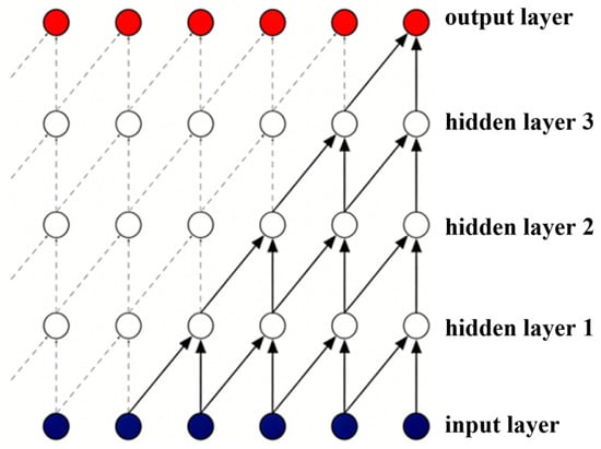
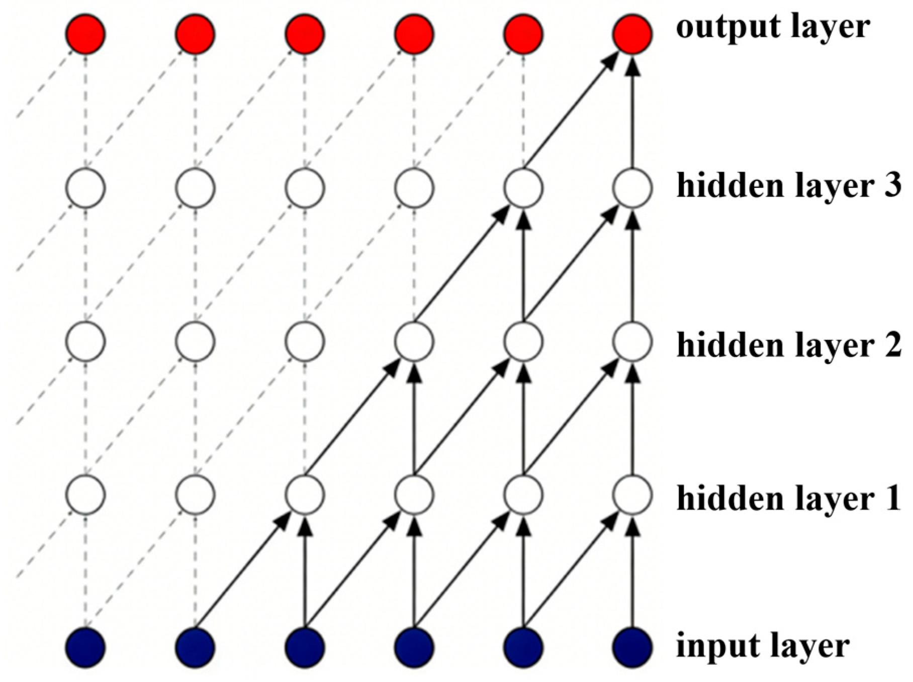
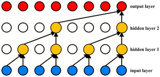
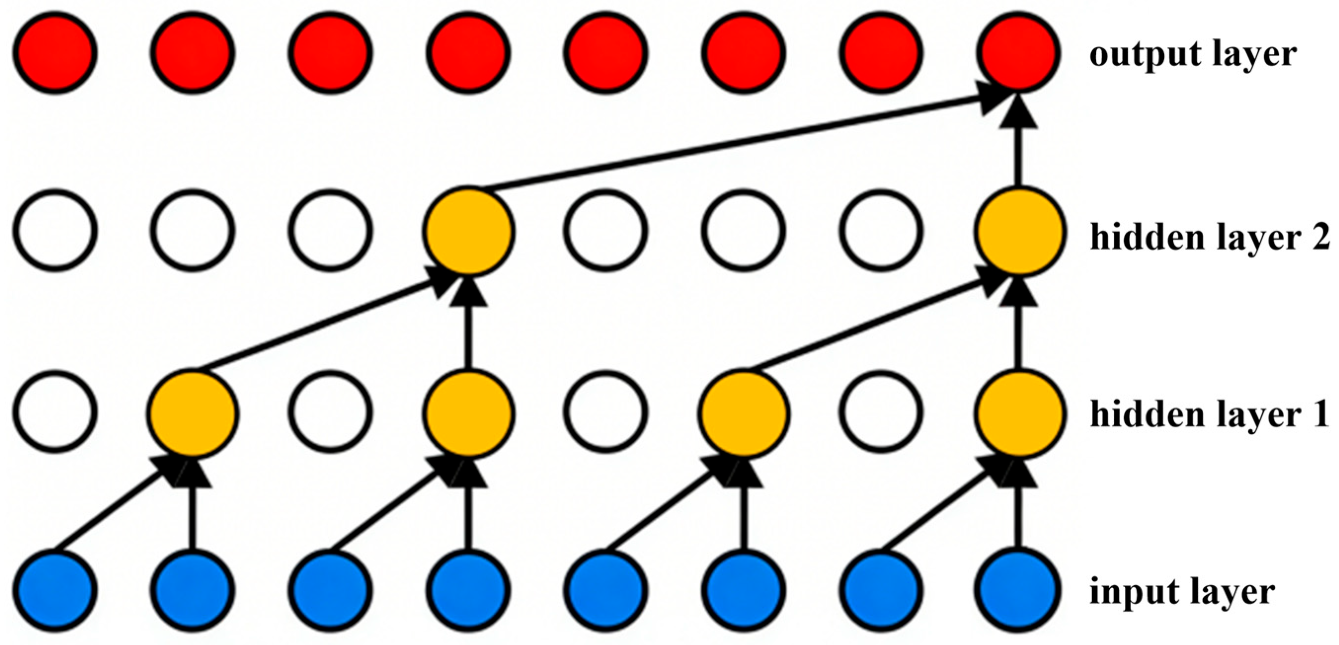
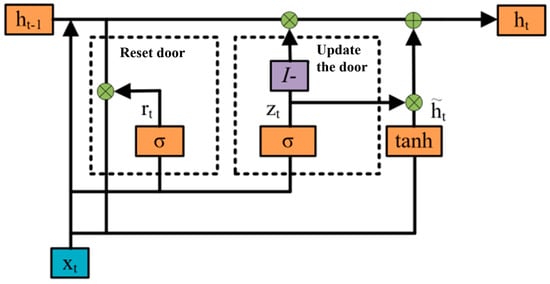
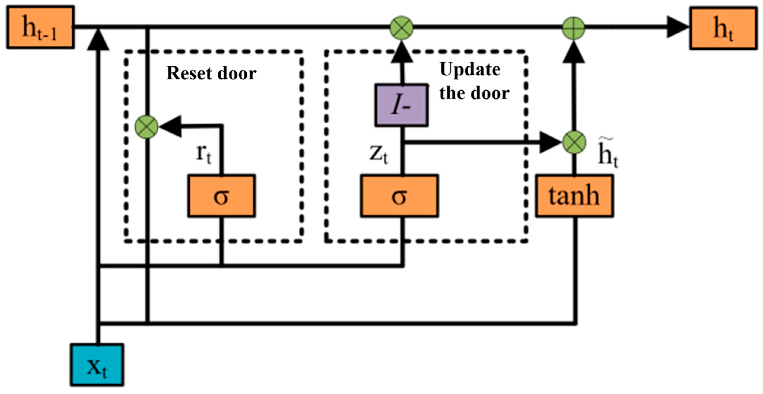
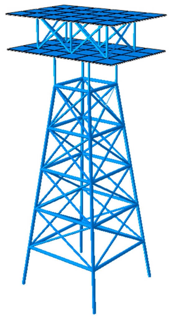
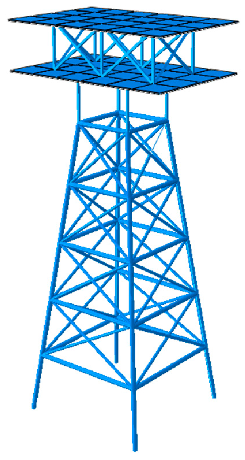
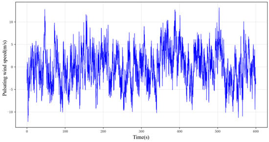
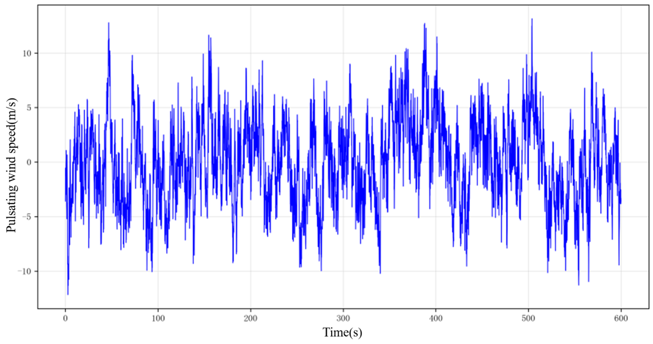
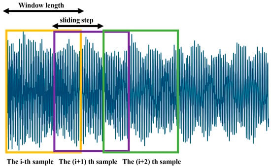
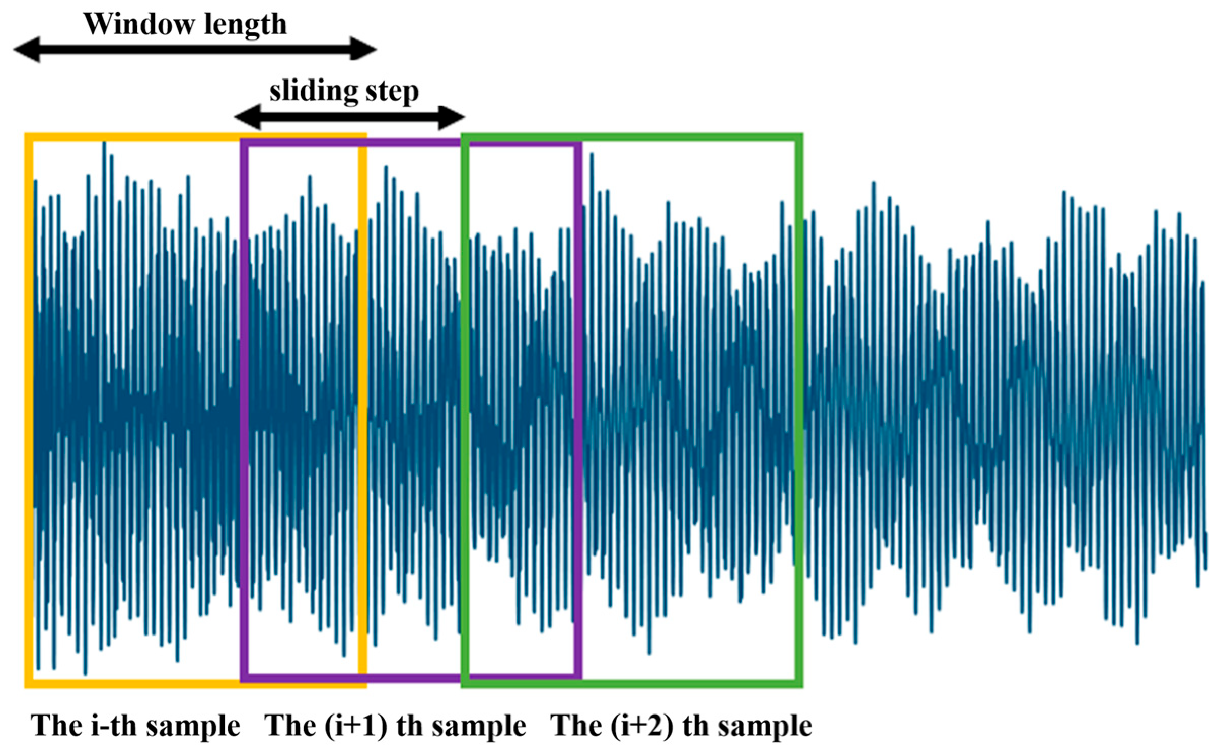
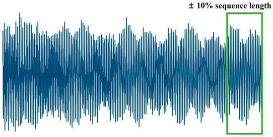
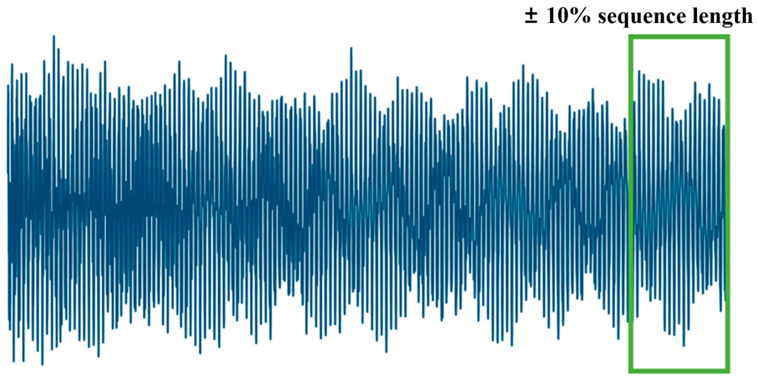
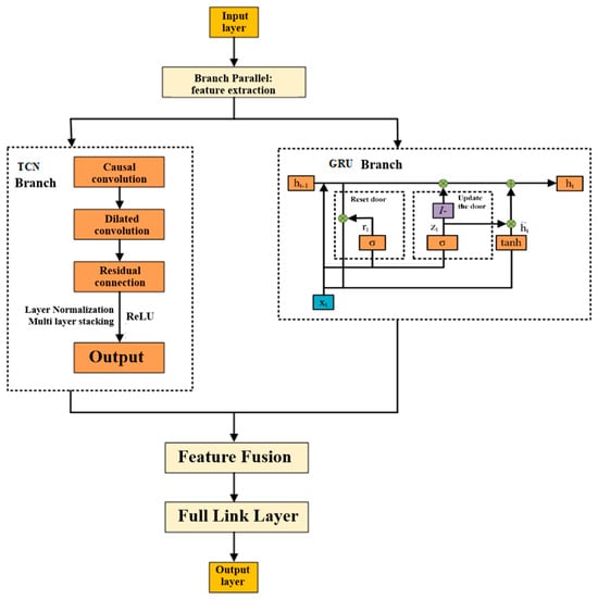
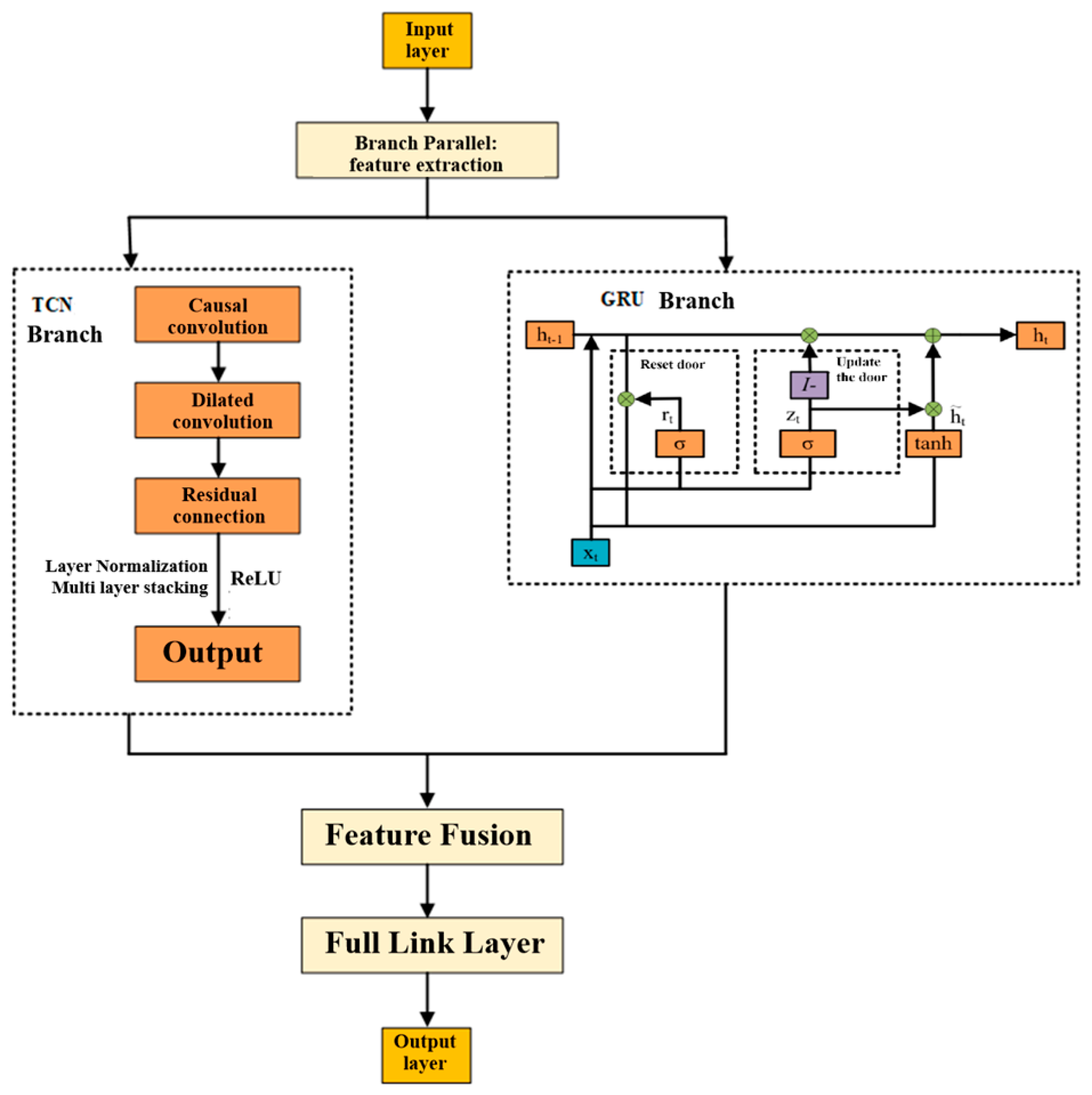
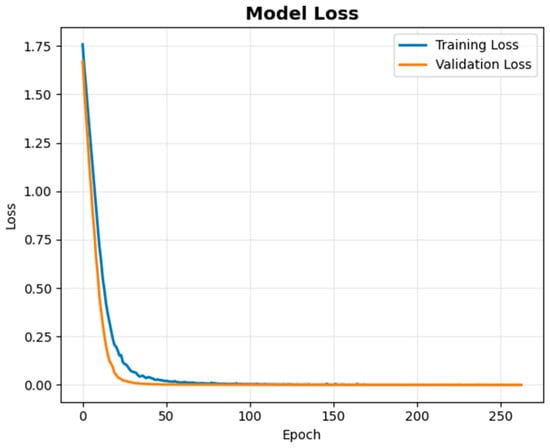
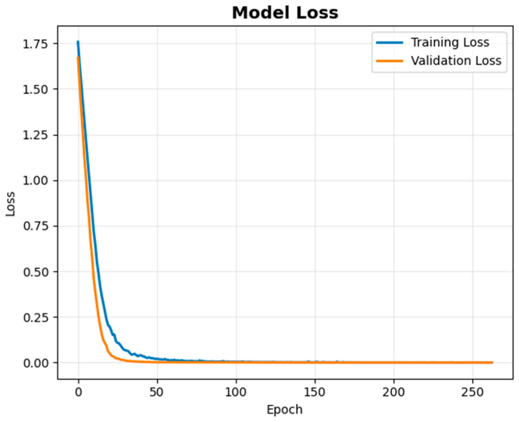
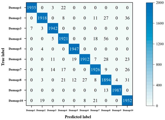
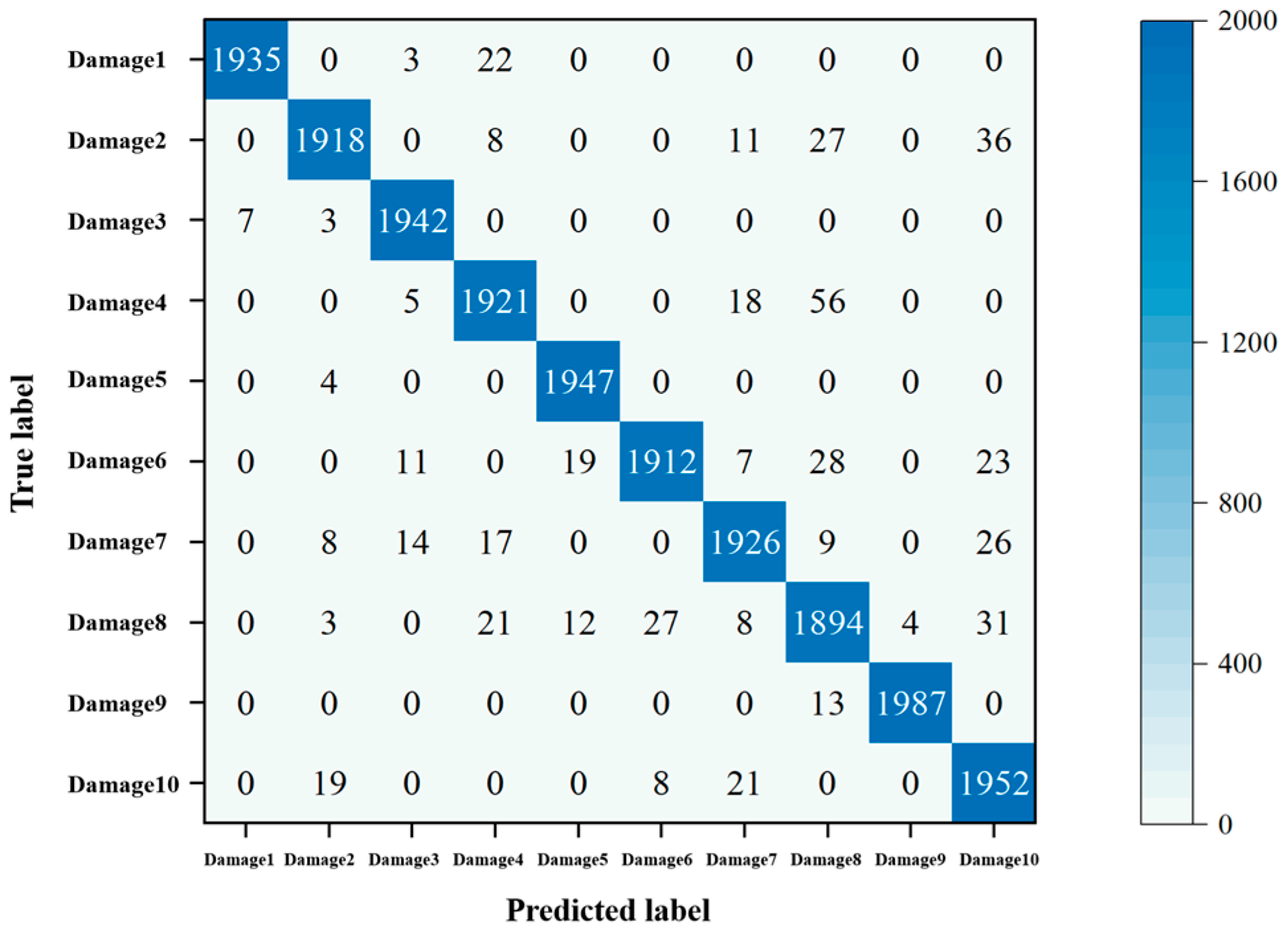
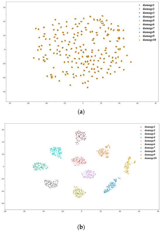
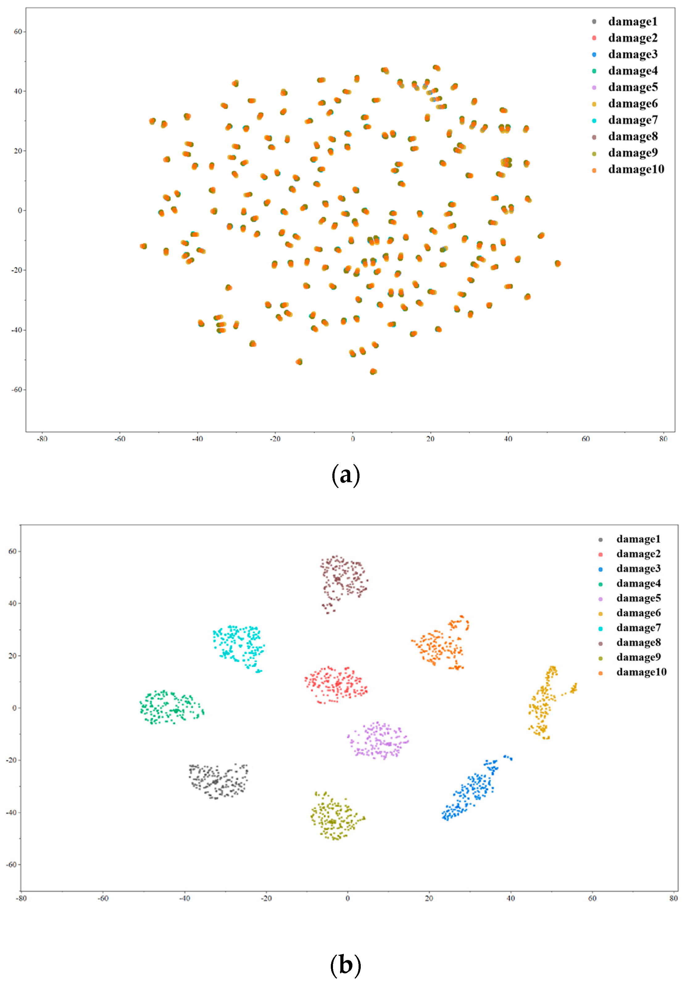
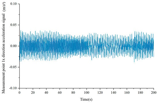
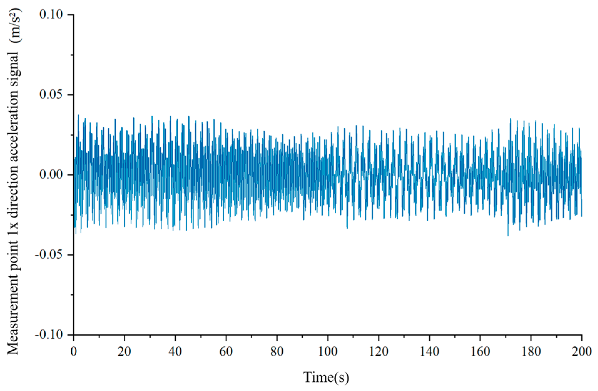
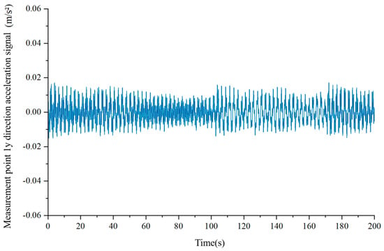
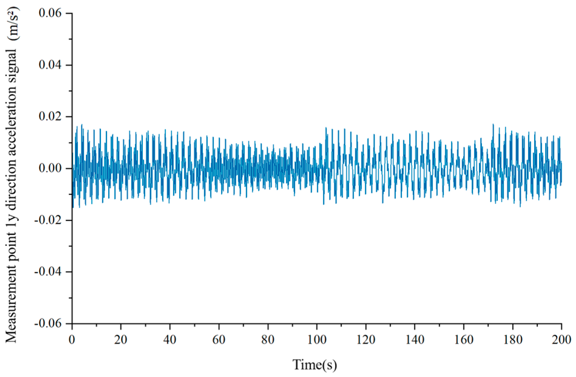
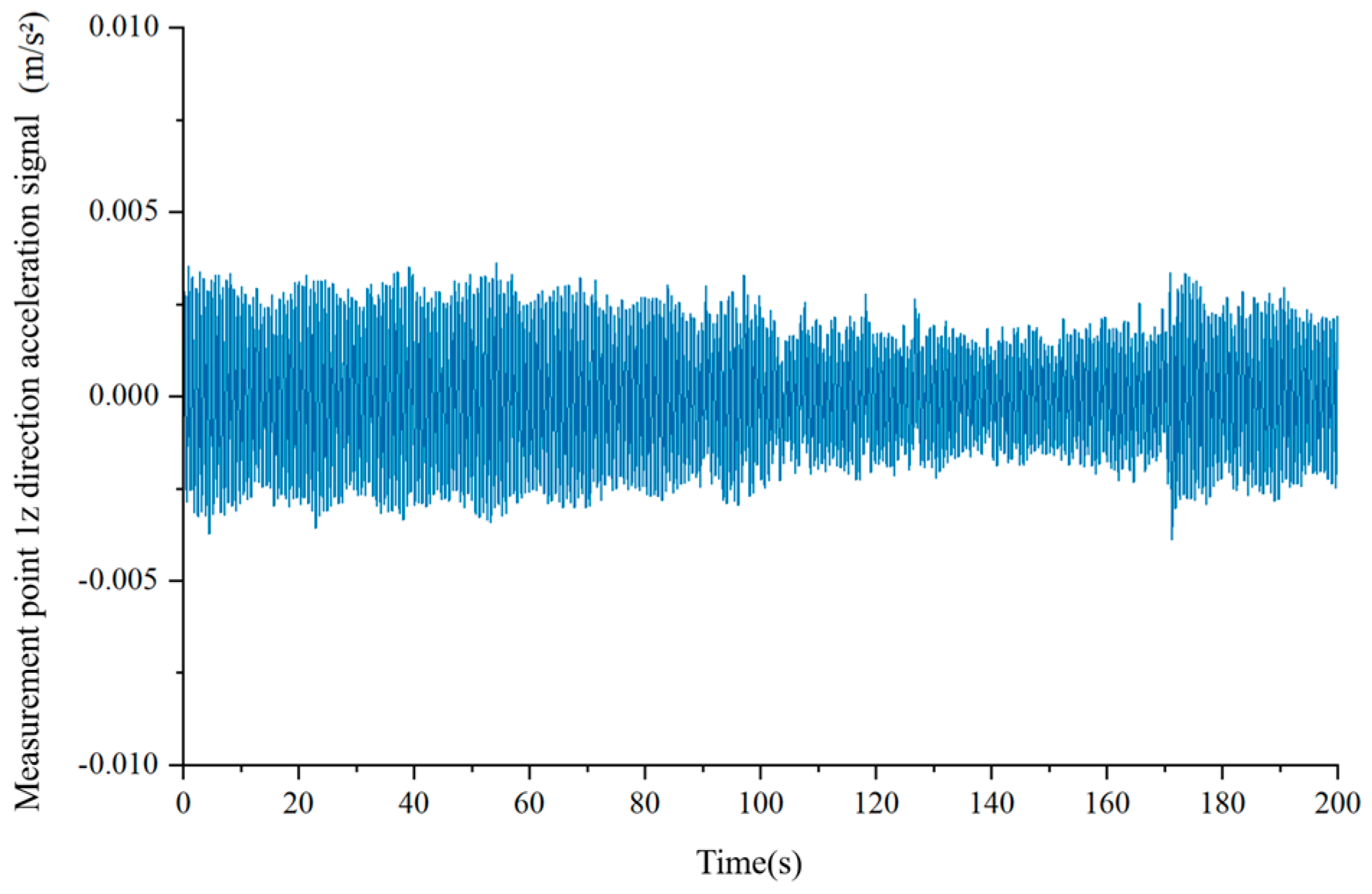
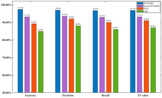
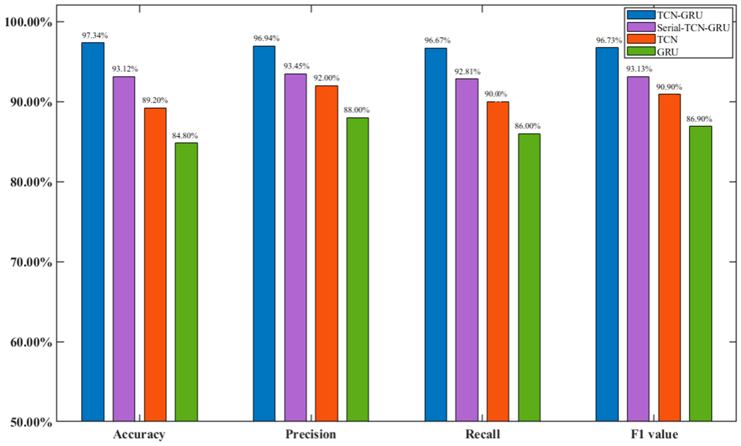
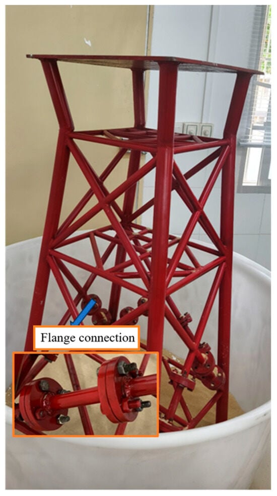
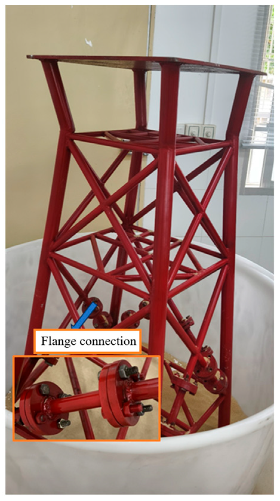
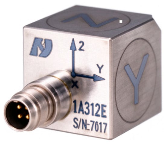
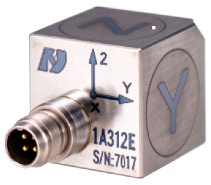
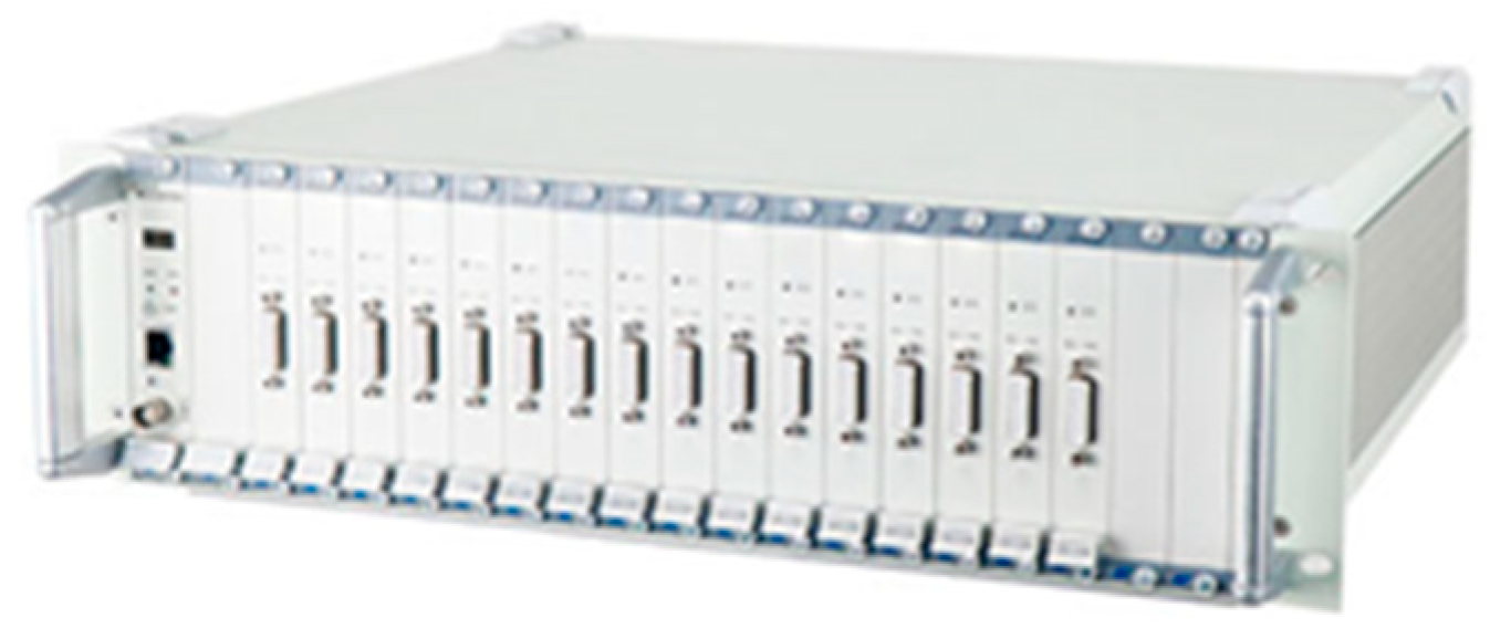
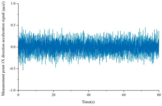
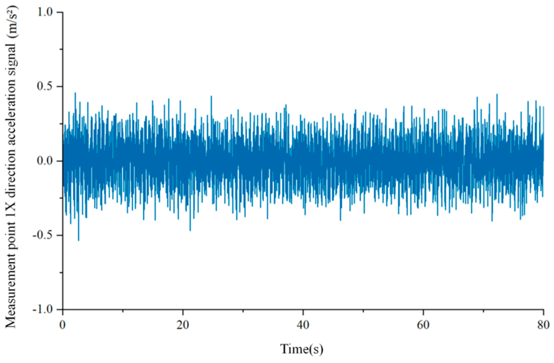
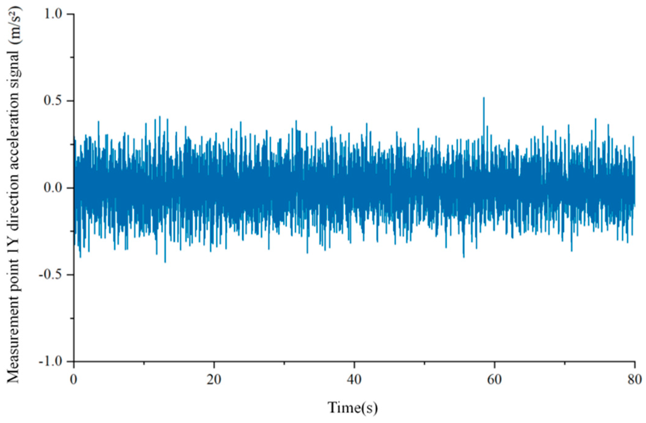
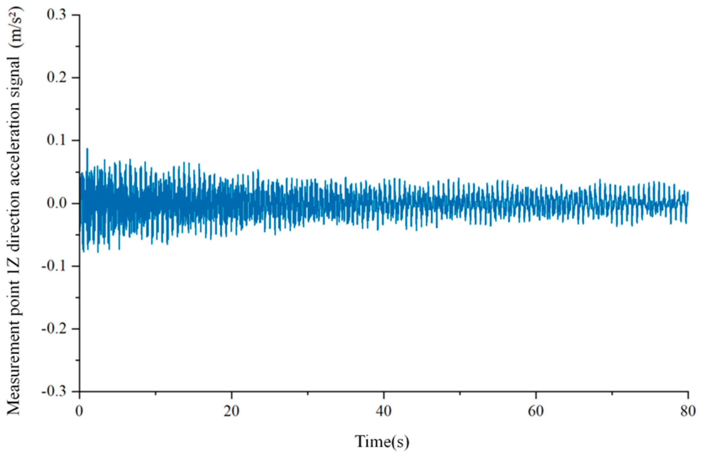
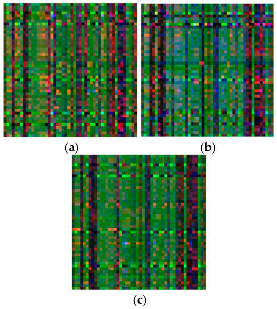
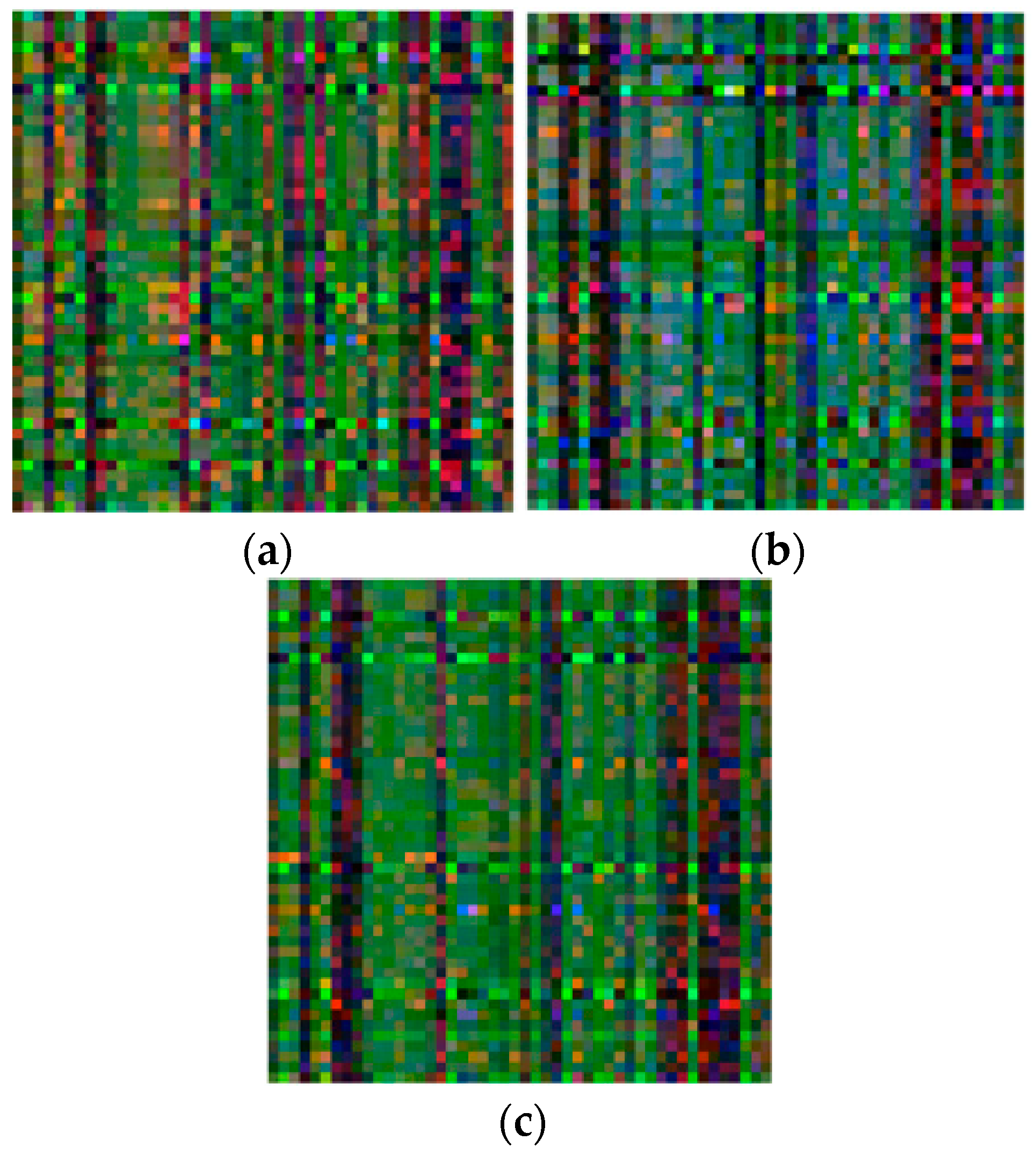
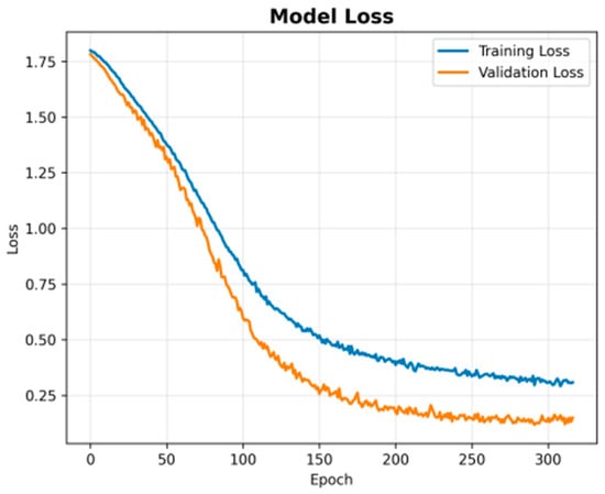
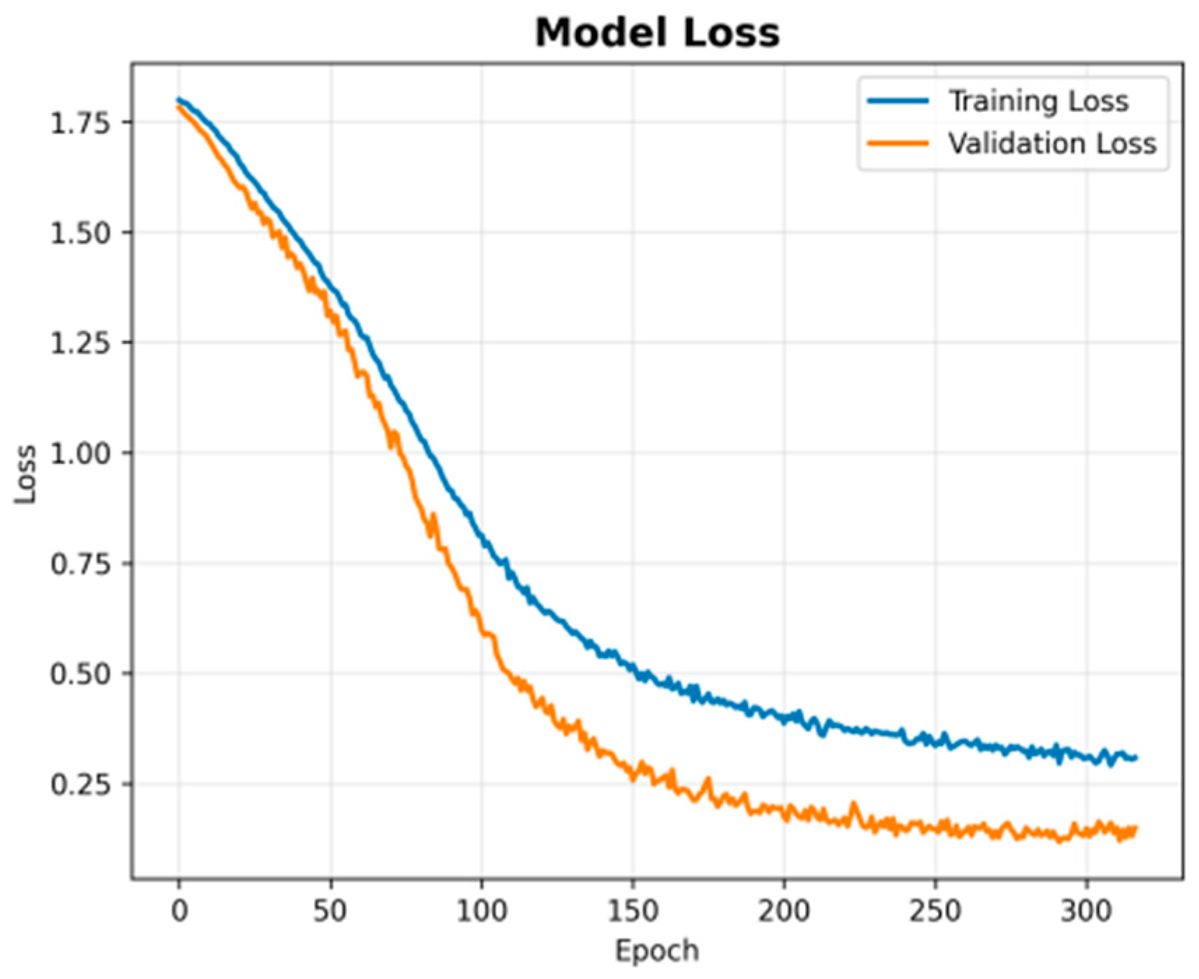
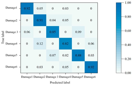
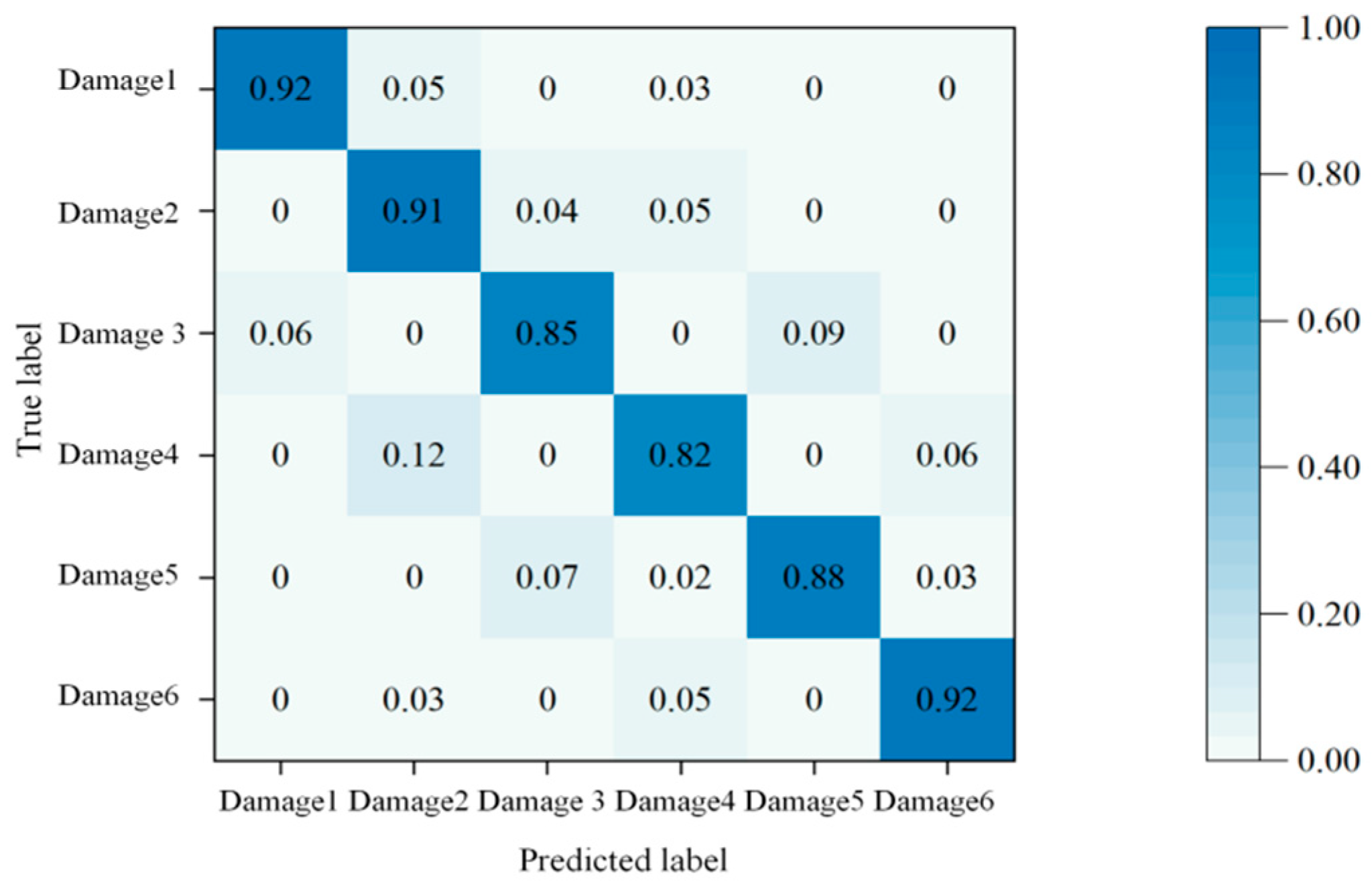

Disclaimer/Publisher’s Note: The statements, opinions and data contained in all publications are solely those of the individual author(s) and contributor(s) and not of MDPI and/or the editor(s). MDPI and/or the editor(s) disclaim responsibility for any injury to people or property resulting from any ideas, methods, instructions or products referred to in the content. |
© 2026 by the authors. Licensee MDPI, Basel, Switzerland. This article is an open access article distributed under the terms and conditions of the Creative Commons Attribution (CC BY) license.