


Abstract
Second-Generation Intact Stability Criteria (SGISC) assess excessive acceleration (EA) through successive vulnerability levels, but the consistency between Level 1 and Level 2 under changes in ship-related parameters remains insufficiently understood. This study investigates the effects of natural roll period, roll damping, and loading condition on both levels. A MATLAB(R2022b)-based implementation was verified using the IMO C11 example and subsequently applied to the ITTC A1, KCS, and DTC container ships. Three levels were assigned to each investigated factor, producing 27 combinations per ship and 81 cases overall. Responses were examined through case-wise comparisons, isolated and paired-factor trends, and a sum-of-squares decomposition of response variability. A total of 72 cases failed EA1 (the remaining 9 were outside IMO applicability), while 50 passed EA2 and 22 failed at both levels; no Level 1 PASS–Level 2 FAIL outcome was obtained. Longer natural roll periods generally lowered EA1 lateral acceleration while increasing the EA2 long-term probability index, whereas increased damping reduced both measures. Loading-condition effects varied markedly among ships, especially in EA2. Pooled contributions further showed a change from natural roll period dominance in EA1 to roll damping dominance in EA2. These results indicate that parameter sensitivity is both level- and ship-dependent. Since none of the investigated cases passed EA1, the assessment of PASS/FAIL-based cross-level consistency was necessarily limited; however, parameter-induced response trends were examined in detail across both levels.
1. Introduction
The conventional stability criteria were substantially based on earlier casualty statistics due to insufficient understanding of dynamic physics in waves [1]. They were structured as deterministic assessment methods, comprising still-water calculations and static stability concepts [2]. One of the most important reasons for International Maritime Organization (IMO) to develop the Second-Generation Intact Stability Criteria (SGISC) was that although the old criteria classified some newer, faster, higher-capacity, and innovatively designed ships—emerging in response to the continuous growth in seaborne cargo volumes [3]—as safe, accidents of such vessels could not be predicted or prevented [4]. On these grounds, a set of new-generation assessment methods that accounts for ship-wave interaction was required; thus, the SGISC were formulated [5].
The SGISC framework consists of five stability failure modes: excessive acceleration (EA), parametric rolling (PR), dead ship condition (DS), pure loss of stability (PL), and surf-riding/broaching (SR). While the conventional criteria provide an overall stability compliance judgment, the SGISC evaluate stability compliance at level of loading conditions and failure modes. The assessment architecture follows a hierarchical structure. Relatively simple Level 1 calculations produce a more conservative opinion on ship stability, whereas progressing to Level 2 and then to direct stability assessment generally reduces this conservatism while increasing the complexity of the calculations and computational power required. This sequence is not mandatory, and a higher-level assessment may be carried out without first completing the lower-level calculations. Instead of merely focusing on the final results of numerical simulations and direct stability assessments, the SGISC further guides in detail how their methods and procedures are to be applied and how they are to be validated. The conventional criteria present a deterministic approach, whereas the SGISC bring probabilistic dimension to stability evaluation. Furthermore, ships that do not meet stability requirements may still be operated maintaining their safety target by following operational guidance and complying with operational limitations. This enables considerable flexibility because a design that would otherwise be rejected on the basis of its fixed characteristics may remain acceptable when loading conditions, environmental conditions, and operational parameters are taken into account [1,5].
The physical background of excessive acceleration (EA), one of the failure modes covered in the SGISC, has been described in the IMO Explanatory Notes [5]. Building on this framework, subsequent studies have shown that the assessed vulnerability depends on a combination of stability characteristics, loading condition, roll dynamics, assessment location, ship geometry, operational state, environmental conditions, and modelling assumptions rather than on a single parameter. Boccadamo and Rosano [6] examined EA vulnerability for four naval hull forms over five displacement conditions. After failing Level 1 (EA1), all investigated conditions required Level 2 (EA2) assessment, where the EA-based lower bound on KG was found to exceed the upper bound imposed by conventional naval intact-stability requirements, eliminating a common admissible stability range for the ships considered. For the largest draught considered, the lower KG boundary obtained from the EA assessment varied between 6.3 and 8.5 m, while naval stability regulations restricted KG to values between 4.81 and 7.42 m. For a 13 K oil/chemical tanker, Shin and Moon [7] examined how roll characteristics, onboard assessment position, and loading-related stability enter the EA evaluation, while their Level 2 analysis also underscored the role of roll damping. At a longitudinal assessment position located at 65% of the ship length from the aft end, Level 1 began to produce failing cases at an assessment height of approximately 50 m, whereas the corresponding Level 2 evaluation remained acceptable up to about 100 m. This dependence on the representation of roll dynamics was also evident in the independent SGISC implementations reported by Marlantes et al. [8], who compared two separately developed computational frameworks and highlighted roll damping as an important source of variability, particularly in EA2. For the C11 container ship case, the two implementations predicted Level 1 lateral accelerations of 1.600 and 1.476 m/s2, respectively, while both yielded the same PASS classification at EA1 and EA2. Turning to operational and environmental effects, Begović et al. [9] adapted the EA Level 2 formulation for simplified operational guidance so that ship speed and wave heading could be explicitly considered. For the bulk-carrier case, the safe operating region contracted as significant wave height (Hs) increased, while the most severe response among the examined conditions occurred at a mean zero-crossing wave period (Tz) of 8.5 s. The resulting weighted fraction of operating conditions to be avoided was 0.017, well below the acceptance limit of 0.20. The influence of hydrodynamic modelling assumptions was investigated by Duan et al. [10] through five alternative approaches applied to the same shallow-draft ship. Their nonlinear five-degree-of-freedom formulation, incorporating modified restoring and diffraction effects, gave the closest agreement with the experiments; the predicted maximum lateral acceleration was 0.837 times gravitational acceleration (g), compared with 0.875 g measured in the model tests. Both values remained below 1 g, consistent with the non-vulnerable outcome obtained from the Level 2 and direct stability assessments. Rosano et al. [11] quantified the influence of damping estimation on EA2 for a stern trawler. When damping derived from roll-decay tests was used, the long-term index was 8.24 × 10⁻⁴, whereas application of the Simplified Ikeda method increased it to 2.26 × 10⁻², approximately 27 times larger. The corresponding equivalent linear damping values were 0.0259 and 0.0108 s−1, respectively, demonstrating how the adopted damping representation can substantially alter the predicted EA response. Experimental evidence of the damping effect was also obtained by Paroka et al. [12] for an Indonesian Ro-Ro ferry using roll-decay tests with and without bilge keels. At Hs = 4.5 m, the vessel without bilge keels satisfied EA2 only when the assessment height was below approximately 55% of the ship breadth, whereas the configuration with bilge keels remained acceptable beyond 80% of the breadth. These results illustrate the substantial enlargement of the acceptable operating and assessment range produced by additional roll damping. Taken together, these studies demonstrate that EA predictions can change appreciably with both physical ship characteristics and the assumptions adopted in the assessment procedure, providing a clear basis for more systematic parameter-sensitivity investigations.
Beyond identifying the factors that influence EA response, attention has also been directed toward quantifying the sensitivity of the assessment to parameter variations. Previous studies have applied the criteria to representative ships and reported the corresponding assessment results. However, the sensitivity of this failure mode to various parameters and the consistency between its assessment levels remain active areas of research. EA vulnerability is sensitive to GM, assessment height, and bilge keel area, since higher GM shortens natural roll period, greater distance from roll axis amplifies lateral acceleration, and weaker damping permits larger roll responses [12]. Kuroda [13] drew on EA Level 1 and EA Level 2 assessment results for 37 vessels previously presented in [14] to examine how GM/B, natural roll period, and normalized assessment height, (h-d)/B, were related to vulnerability. The analysis showed that vessels with GM/B above approximately 0.2 or natural roll periods below 10 s were less likely to be assessed as non-vulnerable, whereas normalized assessment height showed little correlation with the vulnerability outcome. Kuroda subsequently investigated two container ships, referred to as Sample Ships A and B, by varying GM, bilge-keel dimensions, and assessment location at both assessment levels. A 10% reduction in GM, a 50% increase in bilge-keel area, and lowering the assessment location by one deck reduced the Level 1 lateral acceleration by approximately 7%, 10%, and 6%, respectively. At Level 2, the difference between Sample Ships A and B became more pronounced. Sample Ship A satisfied the Level 2 criterion after an approximately 5% reduction in GM, whereas Sample Ship B required a reduction of 37%. Sample Ship A could also satisfy EA2 by increasing the bilge-keel width by 40%, extending its length by 13%, or lowering the assessment location by one deck. For Sample Ship B, increasing the bilge-keel length within the applicable range of the damping method was insufficient; the threshold for non-vulnerability was reached with a 260% increase in bilge-keel width or by lowering the assessment location by four decks. Considering notable influence of draught and vertical center of gravity (VCG) on EA assessment outcomes, Jiang et al. [15] kept these parameters through the preprocessing stage and fed them to machine learning models, while stating that higher assessment locations undergo larger transverse motion, thereby producing bigger accelerations and inertial forces. Within the ±10% perturbation range, increasing VCG reduced the EA probability C, whereas increasing draught produced the opposite trend; moulded depth, in contrast, had only a marginal influence and was excluded from the final EA input set. Qi et al. [16] examined icing-related changes in roll dynamics, found a decrease in linear damping coefficient from 0.0311 to 0.0085 and an increase in nonlinear damping coefficient from 0.1253 to 0.3422 after 24 h of icing, and noted that small damping variations can rapidly alter roll amplitude within the bifurcation region. After a 24-h icing period, the damping level at 0.2 rad/s rose to 1.489 × 10⁸ N.m from an ice-free value of 7.037 × 10⁷ N.m, equivalent to a 111.5% increase. The available evidence therefore indicates that the magnitude of parameter effects can differ substantially among ships and assessment conditions. This raises a further question of whether such variations produce consistent responses across EA1 and EA2.
Beyond parameter sensitivity, the relationship between EA1 and EA2 represents another important aspect of the assessment framework. Since the two levels constitute successive screening stages for the same failure mode, their outcomes are expected to preserve a coherent hierarchy, as intended in the SGISC assessment structure. A further question is whether variations in governing parameters produce comparable response tendencies across EA1 and EA2. Schrøter et al. [17] examined this relationship in an SGISC robustness and consistency study involving 17 vessels. For EA, both levels were evaluated from the light service condition up to summer draught, considering the even-keel, forward, and aft trim conditions, while GM was varied at each draught to identify the GM boundary separating non-vulnerable and vulnerable outcomes at Level 1 and Level 2. Among the 14 vessels for which both EA levels could be compared, 11 showed the expected relationship between the GM limits obtained from Level 1 and Level 2 under all three trim conditions, whereas three did not follow this pattern in at least one trim; usable results were unavailable for the other three vessels. Across the loading conditions, EA1 showed an equal or higher non-compliance rate than EA2 for 13 of the 14 vessels. Ship 13 was the only exception, with none of the examined conditions failing EA1, while 27% failed EA2. Petacco et al. [18] provided a further cross-level comparison by applying both EA vulnerability criteria to 19 loading conditions across seven motor yachts. Based on the reported Level 1 and Level 2 results, three conditions satisfied both levels, eight failed EA1 but satisfied EA2, and eight failed at both levels; no case was accepted by EA1 and subsequently rejected by EA2. These outcomes therefore preserved the expected categorical relationship between the two EA levels throughout the investigated set. Using Gaussian-distributed parameter samples and variance decomposition, Yang [19] investigated the influence of uncertainty in roll characteristics, wave excitation, and assessment location on both EA vulnerability levels. The natural roll period dominated Level 1 (total sensitivity index: 0.80), whereas the effective wave-slope coefficient ranked highest at Level 2 (0.50). The findings further indicated that parameter uncertainty could alter the pass/fail classification for cases approaching the assessment thresholds. A complementary perspective was provided by Duan et al. [20], who investigated the influence of moonpool-related roll damping on both EA assessment levels for an offshore support vessel. Accounting for the reduction in effective roll damping increased the estimated lateral acceleration at Level 1 and the long-term failure probability at Level 2, indicating the same response direction across the two levels for this particular damping-related variation. Previous studies have explored EA cross-level consistency through categorical comparisons of EA1 and EA2 vulnerability classifications, while also documenting how selected parameters influence the assessment results at both levels. However, the consistency of cross-level response trends under systematic, controlled parameter perturbations across vessels with different baseline characteristics remains insufficiently investigated.
Accordingly, this study investigates the sensitivity of EA vulnerability assessment results under controlled variations in loading condition, natural roll period, and roll damping, with particular emphasis on their cross-level consistency. Following validation of the implemented assessment procedures, a common baseline configuration is established and each parameter is varied systematically while the remaining conditions are controlled. The resulting changes in the vulnerability outcomes of both failure levels are then quantified and compared to determine their sensitivity, stability, and relative susceptibility to the imposed variations. This comparison is organized as a three-level full factorial analysis across three benchmark container ships, combining direct adjustments to natural roll period, damping changes applied consistently at both levels, and the hydrostatic consequences of displacement variation. Within this framework, the relative contributions of individual factors and their interactions are quantified for both levels, whereas Kuroda’s [13] investigation of GM, bilge-keel dimensions, and assessment location centers on feasible design measures. Beyond level-specific sensitivity assessment, the study examines whether EA1 and EA2 exhibit consistent trends when subjected to the same changes in ship characteristics. In this way, the work provides a unified basis for distinguishing parameter effects that are consistent across the two assessment levels from those that produce level-dependent responses, thereby contributing to a better understanding of trend-based cross-level consistency of SGISC excessive acceleration assessments.
2. Methodology
This section presents the computational methodology adopted in the present study. Section 2.1 describes the reference ship conditions, parameter variations, and sensitivity analysis framework, while Section 2.2 provides the detailed EA2 computational procedure and numerical settings used to determine the long-term probability index C.
2.1. General Methodology and Sensitivity Analysis
A computational program was developed using MATLAB R2022b to perform the EA1 and EA2 assessments in this study. For each ship, the program takes principal dimensions, loading condition data, hull form offsets, and the vertical and longitudinal positions at which the assessment is carried out as inputs. To investigate how EA1 and EA2 results vary among different ships under changes in loading condition, natural roll period, and roll damping, the original implementation was further modified so that these three quantities could be varied directly through prescribed input values. For loading condition variation, the full-load condition of each ship was first defined as the reference state. The ship’s displacement volume was then reduced to 90% and 80% of its full-load value. Hydrostatic calculations were repeated for these modified loading conditions, and the corresponding updated input parameters were obtained. When the ship’s displacement volume was changed, VCG and longitudinal center of gravity (LCG) were assumed to remain unchanged for simplification. Since redistribution of weights onboard is a complex and case-specific problem, incorporating such effects was considered beyond the scope of the present study and could obscure its primary objective. A more detailed treatment that accounts explicitly for weight redistribution may be considered in future work. For natural roll period (Tr) variation, only the EA1 procedure was modified because Tr is calculated once in the EA1 assessment and the same value is subsequently used throughout the EA2 calculations. Accordingly, a multiplicative natural roll period variation factor, kT, was introduced into Equation (2) of [1] and added to the program inputs, allowing prescribed variations in natural roll period to be imposed systematically.
c = 0.373 + 0.023(B/d) − 0.043(LWL/100)
Here, kT is a dimensionless perturbation factor introduced for the present sensitivity analysis. For each ship and prescribed loading condition, the reference natural roll period is obtained from Equation (2) with kT = 1.00, using the inputs corresponding to that loading state. The values kT = 0.90 and kT = 1.10 impose periods 10% shorter and 10% longer than this reference, respectively, providing symmetric perturbations around the reference value. Within a given loading state, these period changes are imposed without modifying GM or the geometric inputs used in the period calculation. The factor is applied once in calculating the modified period, Tr,var, and the resulting period is subsequently used in both EA1 and EA2. The natural roll frequency in EA2 is derived from this modified period, without an additional application of kT. EA1 and EA2 differ in the way roll damping is represented in their respective assessment procedures. In Level 1, damping is introduced through the non-dimensional logarithmic decrement of roll decay, δφ, whereas Level 2 employs an equivalent linear roll damping coefficient, B44, within the roll-response calculation. To impose consistent roll damping variations at both assessment levels, a single damping variation factor, kB, was introduced as a multiplier applied to the respective damping quantities. For Level 1, using the logarithmic decrement relation given in [5], the modified logarithmic decrement of roll decay (δφ,var) was defined as
whereas for Level 2, the modified roll damping coefficient (B44,var) was obtained from
δφ,var = kB.(0.5πRPR),
B44,var = kB.B44.
Thus, kB was applied to δφ in Level 1 and to B44 in Level 2, allowing the prescribed damping variations to be implemented through a common input parameter.
The independent variations in natural roll period and roll damping were introduced as controlled numerical perturbations rather than as representations of specific physical modifications to the ships. Within a given loading condition, changing the natural roll period while retaining GM and hull geometry can be interpreted as a change in the effective total roll inertia, whereas the damping factor modifies the dissipative contribution to the roll response. Although these characteristics may be physically coupled through changes in loading, mass distribution, and hydrodynamic conditions, treating them separately enables their individual and combined influences on the EA assessments to be distinguished.
The program was applied to four different container ships. One of these was the C11 container ship, which is presented in the IMO Explanatory Notes [5] as an example case for demonstrating the calculation procedure of the excessive acceleration failure mode. The purpose of including C11 was to validate the in-house MATLAB code by comparing the results obtained for this ship with the corresponding IMO results. Further details are provided in the Validation section of the manuscript. Following this validation, the code was applied to three additional container ships considered in the present study. Three benchmark container ships were selected for the present study because their hull forms and principal particulars are publicly available, facilitating reproducibility and independent comparison of the results. The main characteristics of these three ships and of the validation ship C11 are provided in Table 1, while hull forms of the three benchmark ships that constitute the subject of the present study are shown in Figure 1.
Table 1.
Main characteristics of the ITTC A1, KCS, and DTC benchmark container ships and of the validation ship C11.
Figure 1.
Hull forms of ITTC A1, KCS, and DTC.
The original benchmark hull forms were retained, whereas their published reference stability conditions were not treated as fixed constraints for the present EA assessment. The reference conditions available for benchmark vessels are generally defined for specific validation purposes and do not necessarily represent conditions that are particularly informative for excessive acceleration. Since EA vulnerability is strongly influenced by metacentric height and the associated natural roll period, the stability condition of each hull was adjusted to establish a controlled reference state suitable for the present sensitivity analysis. This approach is also consistent with the IMO example application in [5] for the C11 container ship, in which the hull is assessed under a modified stability condition rather than being restricted to its nominal reference values. The adjustment was therefore intended to provide an EA-relevant baseline for systematic comparison, rather than to reproduce an EA assessment for a particular loading condition.
The reference stability conditions for the three benchmark ships were established using the C11 data reported in Tables 1.2 and 3.1 of Reference [5] as a numerical basis. The tabulated KG and GM values give KM = 18.976 + 1.40 = 20.376 m for the basic input condition and KM = 12.75 + 8.00 = 20.750 m for the EA assessment condition. The ratio 20.750/20.376 = 1.018 was first applied to the original KM of each benchmark ship. A provisional GM was then obtained by multiplying the transformed KM by the GM/KM ratio of the C11 EA condition, 8.00/20.750 = 0.386.
For ITTC A1, the original KM of 11.635 m therefore yielded a transformed KM of 11.849 m and a provisional GM of 4.568 m. An additional common multiplier of 1.313 was selected to obtain an ITTC A1 reference GM of approximately 6.00 m. The complete calculation for this ship was thus GM = 1.313 × (8.00/20.750) × (20.750/20.376) × 11.635 ≈ 6 m. Applying the same multiplier to KCS and DTC established a common final GM/KM ratio of 1.313 × 0.386 = 0.506. The corresponding VCG values were determined by subtracting the final GM from the transformed KM. The adjusted full-load stability conditions were subsequently used as the reference for hydrostatic calculations at the reduced displacement levels. The corresponding KM, VCG, and GM values for all three loading conditions of each ship are presented in Appendix A (Table A1). The IMO Explanatory Notes [5] specify that the basic C11 input accounts for the free-surface correction, whereas the EA assessment condition reports GM without this correction. However, the document does not explicitly explain the difference between the corresponding KM values; therefore, their ratio was adopted as a numerical scaling reference for establishing the baseline stability conditions rather than as a physically derived hydrostatic correction.
Once these reference conditions had been defined, displacement volume variations were introduced independently for each ship. For each prescribed displacement volume variation, hydrostatic properties were recalculated at corresponding equilibrium draught, while both VCG and LCG were kept unchanged. Consequently, changes in hydrostatic KM resulting from displacement volume variation were reflected directly in corresponding GM through GM = KM − VCG. This procedure allowed hydrostatic influence of the displacement volume variation to be examined without introducing additional assumptions regarding redistribution of weight in either vertical or longitudinal direction.
To enable a meaningful comparison among the three ships, lateral acceleration assessment location was transferred from the C11 reference case using non-dimensional geometric ratios. The ratios hk/D and x/L [5] were first determined from the C11 reference case and then used for the ships studied in the present work. Accordingly, the vertical (VCA) and longitudinal (LCA) assessment locations for ITTC A1, KCS, and DTC were obtained by applying these C11-based ratios to the depth and length of each ship, respectively.
Natural roll period and roll damping variations were introduced by applying variation factors kT and kB, respectively, with values of 0.90, 1.00, and 1.10. Loading condition variation was generated by reducing the full-load displacement volume of each ship to 90% and 80%. The variation ranges were selected to investigate controlled changes near the reference conditions, while limiting the possibility of substantial shifts in the underlying roll-response characteristics that larger variations might introduce. A common increment of 0.10 was adopted for all three factors, with displacement progressively reduced from the full-load condition, providing a consistent relative scale for examining parameter-induced changes. Full factorial combination of these three variation sets yielded 27 analysis cases for each ship. Accordingly, a total of 81 cases were evaluated for ITTC A1, KCS, and DTC. The configuration of individual cases and complete set of resulting outputs are presented in Appendix Figure A1.
To aid interpretation of the computed responses, the 27-case design for each vessel was decomposed with respect to three prescribed factors: loading condition, natural roll period variation factor kT, and roll damping variation factor kB. The decomposition considered the individual contributions of the three factors, the three pairwise combinations, and the joint three-factor combination. Since only one computed response was available at each point of the 3 × 3 × 3 design, no residual degrees of freedom remained for conventional inferential ANOVA; therefore, F-ratios and p-values were not evaluated. Instead, the sum-of-squares contribution of each component was normalized by total sum of squares and reported as a percentage. This provided a descriptive measure of the contribution of each factor or interaction to the variation in the calculated response across the 27 cases of each ship. The procedure was carried out independently for Level 1 lateral acceleration ay and Level 2 long-term probability index C. The ANOVA-based variance decomposition adopted in this study was formulated as follows (Equations (5)–(20)) [21]. Let yijk denote calculated response corresponding to the ith loading condition, the jth level of kT, and the kth level of kB, where each of i, j, and k ranges from 1 to 3.
Overall mean:
Factor-level means:
Two-factor combination means:
Main-effect sums of squares:
Two-way interaction sums of squares:
Total sum of squares:
Three-way interaction sum of squares:
SSLTB = SSTotal − SSL − SST − SSB − SSLT − SSLB − SSTB
Percentage contribution to total variation:
All figures presented in this study were generated in MATLAB using the actual data obtained from the computations.
2.2. EA2 Computational Procedure and Numerical Settings
The EA2 vulnerability assessment was implemented in accordance with Section 2.3.3 of Reference [1], with the supplementary procedures for effective wave slope estimation and roll damping based on Appendix 3 of Reference [5], particularly Sections 8.2 and 9.2–9.3. For each investigated ship and loading condition, the calculation involved determining the frequency-dependent roll response and lateral acceleration, evaluating the short-term excessive acceleration failure index for each sea state, and combining these indices according to their occurrence weights to obtain the long-term probability index characterizing vulnerability to excessive acceleration, C. The governing equations, environmental conditions, numerical discretization, and modeling assumptions adopted in the present implementation are detailed below to facilitate reproducibility.
The environmental conditions considered in the EA2 calculations were defined using the North Atlantic-based standard wave scatter table for unrestricted service provided in Section 2.7.2.1.2 of Reference [1]. The computational grid comprised 17 significant wave heights (Hs = 0.5–16.5 m) and 18 mean zero-crossing wave periods (Tz = 1.5–18.5 s), both with increments of 1.0 m and 1.0 s, respectively. The two additional wave-period columns (Tz = 1.5 and 2.5 s), which are omitted from the published scatter table, were retained in the numerical implementation with zero occurrence weights. For each sea state, the weighting factor Wi was calculated by dividing the corresponding occurrence count by 100,000, ensuring that the sum of all weights equals unity. The wave elevation spectrum associated with each sea state was represented using the Bretschneider formulation specified in Section 2.7.2.1.1 of Reference [1].
For each sea state, the frequency-dependent spectral density of wave elevation was calculated using the following expression [1]:
where Szz(ω) is the wave elevation spectral density (m2/(rad/s)), Hs denotes the significant wave height (m), Tz represents the mean zero-crossing wave period (s), and ω is the circular wave frequency (rad/s).
The frequency integration range was determined separately for each investigated case using its natural roll period, following Section 2.3.3.2.2 of Reference [1]. The lower and upper frequency limits, frequency increment, and midpoint frequencies were defined as follows:
where ω1 and ω2 are the lower and upper frequency limits (rad/s), respectively; ∆ω denotes the frequency increment (rad/s); Tr is the natural roll period (s); and ωj represents the midpoint frequency of the jth interval. The number of frequency intervals was set to Nω = 1000, with j ranging from 1 to Nω. This discretization was applied consistently to all sea states, while the frequency limits were updated according to the natural roll period of each case.
The effective wave slope function, r(ω), was evaluated at each discretized wave frequency using the standard methodology presented in Section 8.2 of Appendix 3 in Reference [5]. This procedure represents the submerged hull geometry through equivalent underwater sections, constructed from the sectional area, waterline breadth, and draught obtained from the hull offset data. The resulting frequency-dependent effective wave slope function was then used to determine the wave-induced Froude–Krylov roll exciting moment. The effective wave slope function was obtained by integrating the sectional contributions along the ship length and normalizing the resulting integral by the equivalent displacement volume and metacentric height [5]:
Here, C(x) represents the contribution of each equivalent section to the longitudinal integration, while ∇eq denotes the underwater volume of the equivalent hull. These quantities were evaluated from the sectional geometry using the formulations provided in Section 8.2.2–8.2.3 of Reference [5]. For the laterally symmetric hulls considered in this study, the cosine and sine components of the Froude–Krylov roll exciting moment were calculated using the simplified relations given in Section 8.3.3 of Reference [5]:
where a(ω) and b(ω) denote the cosine and sine components of the Froude–Krylov roll exciting moment per unit wave amplitude (kN·m/m), respectively; ρ is the seawater density (kg/m3); and ∇ denotes the displacement volume (m3). For the EA2 roll-response calculations, the Simplified Ikeda method was employed to obtain the total roll damping coefficient from its individual contributions [5]:
where BF, BW, BE, BL, and BBK represent the contributions from skin friction, wave making, eddy making, lift, and bilge keels, respectively. The damping coefficient was evaluated across the wave-frequency range at a prescribed roll amplitude of 15°. This fixed amplitude is permitted as an alternative to stochastic linearization under Section 9.3.8 of Appendix 3 in Reference [5], and is also employed in the C11 validation example presented in Section 3.3.1 of Appendix 2 in Reference [5]. Since the EA2 calculations were performed at zero forward speed under beam-sea conditions (waves incident perpendicular to the ship’s centerline), the speed-dependent lift contribution was taken as zero (BL = 0). The calculations were performed using a seawater density of 1025 kg/m3, a kinematic viscosity of 1.16 × 10⁻⁶ m2/s, and a gravitational acceleration of 9.81 m/s2.
B44 = BF + BW + BE + BL + BBK
For each ship and loading condition, the baseline EA2 roll damping was calculated using the Simplified Ikeda method with the corresponding hull geometry, bilge-keel characteristics, and hydrostatic inputs at kB = 1.00. The damping variation factors defined in Section 2.1 were subsequently applied to these calculated coefficients, rather than to experimentally measured damping values.
To maintain dimensional consistency with the roll-response equations, the modified damping coefficient was converted from N·m·s to kN·m·s as follows:
The total roll moment of inertia, including the added-inertia contribution, was determined from the natural roll period and hydrostatic restoring characteristics in accordance with Section 2.3.3.2.2 of Reference [1]:
with JT,roll expressed in t·m2, the frequency-dependent cosine and sine components of the roll response, φr and φi (rad/m), were calculated according to Section 2.3.3.2.2 of Reference [1]:
The roll response amplitude per unit incident wave amplitude, φa(ω) (rad/m), was obtained by combining the two response components [1]:
The lateral acceleration response per unit wave amplitude at the specified assessment location was then calculated from the roll amplitude using the following relation [1]:
where kL accounts for the simultaneous effects of roll, yaw, and pitch motions, and hr is the vertical distance between the roll axis and the acceleration assessment location (m). The resulting ay(ω) is expressed in (m/s2)/m.
ay(ω) = kL(g + hrω2)φa(ω)
For each sea state, the variance of lateral acceleration was determined by integrating the squared acceleration response over the corresponding wave spectrum, using the midpoint discretization defined in Equation (22) [1]:
The factor 3/4 accounts for the influence of wave short-crestedness, while the resulting standard deviation, σLA,i, is expressed in m/s2.
For the subsequent spectral comparison, the lateral-acceleration spectral density is defined as
corresponding to the frequency-dependent integrand of Equation (31) for a specified sea state.
For each sea state, the short-term excessive acceleration failure index was calculated as follows [1]:
where R2 = 9.81 m/s2 is the prescribed lateral acceleration threshold. The resulting CS,i is dimensionless and represents the probability of exceeding this threshold under the corresponding sea state.
The long-term probability index C was subsequently obtained by summing the weighted short-term failure indices across the entire sea-state grid [1]:
Here, Ns = 306 corresponds to the 17 × 18 sea-state combinations considered in the numerical implementation, including those assigned zero occurrence weights.
The resulting long-term probability index was evaluated against the EA2 acceptance threshold of REA2 = 3.9 × 10⁻⁴, as specified in Section 2.3.3.1 of Reference [1]. A loading condition was classified as non-vulnerable at Level 2 when C ≤ REA2; otherwise, it was classified as potentially vulnerable to excessive acceleration.
The principal numerical settings and computational assumptions adopted in the EA2 assessment are summarized in Table 2.
Table 2.
Summary of numerical settings adopted in the EA2 calculations.
The transverse hull sections used in the EA2 calculations were extracted from the three-dimensional IGES hull models of ITTC A1, KCS, and DTC, obtained from the corresponding benchmark data sources [22,23,24]. For each ship, 39 sections distributed along the hull length were adopted as the reference discretization. The 39-section arrangement was selected based on naval architectural judgment, incorporating half-stations near the bow and stern to better capture the rapid changes in hull geometry in these regions.
To examine the numerical convergence of the EA2 calculations with respect to frequency discretization, 14 cases were selected from the complete dataset based on their proximity to the acceptance threshold, using a relative band of ±15% (0.85 ≤ C/REA2 ≤ 1.15). This subset comprised ITTC A1 Cases 16, 22, and 26; KCS Cases 1, 5, 8, 11, 18, and 21; and DTC Cases 4, 7, 13, 16, and 22, with seven calculated EA2 indices below and seven above the acceptance limit. Each case was recalculated using 500, 1000, 2000, and 4000 frequency intervals, yielding 56 calculations while retaining the same 39 transverse hull sections and all other prescribed input parameters. The relative percentage difference in the EA2 long-term probability index was determined by comparing each frequency discretization with the corresponding result obtained using 4000 intervals, which served as the finest-resolution numerical reference. Across the 14 cases, the maximum relative differences were 2.14 × 10⁻⁸%, 5.10 × 10⁻⁹%, and 1.00 × 10⁻⁹% for 500, 1000, and 2000 intervals, respectively, with all three maxima occurring for KCS Case 21. The deviations decreased systematically with increasing frequency resolution. Furthermore, the results obtained using the original 1000-interval discretization reproduced the reported C values, within their displayed precision, and none of the investigated cases changed its EA2 vulnerability classification. These results demonstrate that the adopted frequency discretization provides numerically stable long-term probability estimates for the investigated cases near the EA2 acceptance boundary, with negligible differences relative to the finest resolution examined.
Unlike the negligible changes observed when refining the frequency integration grid, the number of transverse hull sections had a more discernible influence on the EA2 long-term probability index, reflecting the role of sectional geometry in the longitudinal integration of the effective wave slope. The same 14 cases near the EA2 acceptance threshold were evaluated using 20, 39, 77, and 153 sections, with the frequency discretization fixed at N = 1000 and all case-specific inputs unchanged. Relative to the original 39-section representation, the mean absolute deviations in C were 1.76%, 0.57%, and 0.57% for 20, 77, and 153 sections, respectively, while the largest deviation at 153 sections was 1.25%. The maximum difference between the 77- and 153-section results was only 0.135%, indicating numerical stabilization at finer sectional resolutions despite some non-monotonic differences relative to the original representation. All 14 cases retained their original EA2 vulnerability classifications at both finer resolutions. However, the 20-section representation produced a classification reversal for DTC Case 13, increasing C by 5.62% relative to the 39-section result and shifting the normalized index C/REA2 from 0.9578 (PASS) to 1.0117 (FAIL). At 77 and 153 sections, the corresponding ratios were 0.9696 and 0.9686, respectively, both remaining below the acceptance limit. This isolated reversal highlights the sensitivity of threshold-adjacent EA2 assessments to coarse hull discretization, whereas the close agreement between the finer representations supports the numerical stability of the results without implying strictly monotonic convergence toward the original 39-section values.
3. Validation
This section presents validation of the MATLAB program developed and used in the present study. For this purpose, the program was run for the C11 container ship, which is used in IMO Explanatory Notes [5] as the example vessel for excessive acceleration assessment. Results obtained from the present implementation were then compared with the corresponding IMO results. The main characteristics of the C11 container ship are summarized in Table 1.
A direct comparison between EA1 results obtained from the in-house code and those reported in the corresponding IMO calculations is presented in Table 3.
Table 3.
Percentage differences between calculated EA1 results and IMO results for C11 [5].
The wave frequency-dependent equivalent linear roll damping coefficient used to represent roll damping in EA2 calculations is shown in Figure 2 for a roll amplitude of 15°. The Figure presents both values obtained from the developed computational code and the corresponding results reported for the IMO example ship, allowing a direct comparison between two implementations.
Figure 2.
B44 validation comparison at 15° degrees of roll [5].
The effective wave slope coefficient used in the Froude–Krylov roll moment calculation is plotted against wavelength-to-ship-breadth ratio in Figure 3. For validation purposes, both the in-house code and the corresponding IMO are plotted together in the same figure.
Figure 3.
Effective wave slope coefficient validation comparison [5].
Finally, Table A4 in Appendix B presents percentage differences between the standard deviation of lateral acceleration values, σLAi, obtained from the in-house MATLAB code, and the corresponding IMO results [5]. The relatively large percentage differences in the first few rows of the Tz = 1.5 s column are mainly attributable to rounding of very small numerical values. The systematic differences observed at Tz = 2.5 and 3.5 s may be associated with minor differences in the frequency-dependent lateral acceleration calculations, particularly in the effective wave slope estimation at shorter wavelengths, where a slight discrepancy between the curves is visible in Figure 3. For the Bretschneider wave spectrum adopted in the EA2 assessment, Szz is proportional to Hs2, and consequently, σLA is proportional to Hs at a fixed Tz, explaining why these relative differences remain nearly constant across wave heights. Two underlying σLAi tables, Table A2 and Table A3, are provided in Appendix B for direct inspection and comparison.
For EA2, the long-term probability index calculated for the C11 container ship was C = 4.65949 × 10⁻⁴, compared with the IMO reference value of C = 4.70000 × 10⁻⁴ [5], corresponding to a relative difference of approximately 0.86%. Both values exceed the acceptance limit of REA2 = 3.9 × 10⁻⁴, yielding the same vulnerability classification.
Taken together, the results obtained by applying the in-house code to the C11 container ship show close agreement with the corresponding IMO results.
Another important validation check of the program is presented in Figure 4, Figure 5 and Figure 6. For each ship and each individual case, frequencies corresponding to maximum roll angle and maximum lateral acceleration are located in the vicinity of the natural roll frequency, providing an additional consistency check on the calculated responses.
Figure 4.
Natural roll frequency and the frequencies corresponding to the maximum roll angle and maximum lateral acceleration for each ITTC A1 case.
Figure 5.
Natural roll frequency and the frequencies corresponding to the maximum roll angle and maximum lateral acceleration for each KCS case.
Figure 6.
Natural roll frequency and the frequencies corresponding to the maximum roll angle and maximum lateral acceleration for each DTC case.
4. Results
EA1 and EA2 assessments were performed using the in-house MATLAB code for the benchmark container ships ITTC A1, KCS, and DTC, whose principal characteristics and three-dimensional hull forms are presented in Table 1 and Figure 1, respectively. The corresponding results are presented in this section. The IMO applicability conditions were considered separately from the numerical EA1 and EA2 assessments. According to Section 2.3.1.1 of Reference [1], ITTC A1 Cases 19–27, corresponding to the full-load condition, fall outside the EA applicability range at the adopted assessment location, since the height above the waterline (18.40 m) is below the required 70% of the ship breadth (19.04 m), although the GM requirement is satisfied. Nevertheless, these nine cases were retained in the numerical analysis to preserve the complete three-level factorial design. Their exclusion would eliminate an entire loading level for ITTC A1, preventing consistent evaluation of loading effects and their interactions with natural roll period and roll damping, as well as direct comparison with the other two ships. Retaining these cases also allows the calculated responses to be examined across the full prescribed displacement range without truncation at the applicability boundary. Accordingly, all 81 cases were included in the numerical sensitivity analyses and figures, whereas the applicability-based PASS/FAIL statistics were restricted to the remaining 72 cases. For the nine excluded cases, the reported EA1 and EA2 classifications represent numerical threshold comparisons rather than formal IMO vulnerability assessments. As a first overview, Figure 7 shows EA1 lateral acceleration response, ay (m/s2), and EA2 long-term probability index, C, for the 27 cases defined for each ship, giving a total of 81 cases. Case matrix comprises three loading conditions, three natural roll period variations, and three roll damping variations, as described in the Methodology section. The vulnerability limits REA1 = 4.64 (m/s2) and REA2 = 0.00039 are also indicated in Figure 7 to facilitate direct identification of the cases approaching or exceeding the corresponding assessment thresholds.
Figure 7.
Scatter plot of EA1 lateral acceleration and EA2 long-term probability index for all 81 cases, with the corresponding REA1 = 4.64 (m/s2) and REA2 = 0.00039 vulnerability thresholds.
Because case numbering follows a structured progression of the prescribed variations, the sequence itself provides additional information that can be observed with Figure A1 in Appendix A. Figure 8 therefore presents EA1 lateral acceleration and EA2 long-term probability index values from Case 1 to Case 81 as line plots for the three ships. Case 1 corresponds to a loading condition factor of 0.80, a natural roll period factor of 0.90, and a roll damping factor of 0.90. Within each loading condition, the damping factor changes first from 0.90 to 1.00 and 1.10. The natural roll period factor is then advanced from 0.90 to 1.00 and 1.10, with the same damping sequence repeated at each level. After all combinations for the 0.80 loading condition are completed, the procedure continues with the 0.90 loading condition and then with the 1.00 loading condition following the same ordering. This case structure is applied identically to ITTC A1, KCS, and DTC.
Figure 8.
Line graph of EA1 lateral acceleration and EA2 long-term probability index for all 81 cases.
Figure 9 presents isolated effects of variations in natural roll period, roll damping, and loading condition on EA1 lateral acceleration and EA2 long-term probability index. For each variation, one parameter is changed while the other two are held constant, allowing the individual response associated with each parameter to be displayed separately. Each ship is represented by a different colored line, with EA1 results shown in the upper row and EA2 results in the lower row.
Figure 9.
Isolated variation effects of natural roll period, roll damping, and loading condition on EA1 lateral acceleration and EA2 long-term probability index for the ITTC A1, KCS, and DTC benchmark container ships.
The combined effects of two varying parameters are presented as response surfaces in Figure 10 and Figure 11. For each surface, one parameter is fixed at its reference value of 1.00, while the cases corresponding to variations in other two parameters are used to construct the plotted response. Figure 10 shows EA1 lateral acceleration, whereas Figure 11 presents EA2 long-term probability index. These response patterns are discussed in detail in the Discussion section.
Figure 10.
Two-factor response surfaces of EA1 lateral acceleration for ITTC A1, KCS, and DTC, with the third parameter fixed at its reference value of 1.00.
Figure 11.
Two-factor response surfaces of EA2 long-term probability index for ITTC A1, KCS, and DTC, with the third parameter fixed at its reference value of 1.00.
Relative influence of the investigated parameters on computed EA responses is summarized through the variance-decomposition results in Table 4 and Table 5. Table 4 presents the percentage contributions of the main effects of loading condition, the natural roll period factor kT, and the roll damping factor kB, as well as the three pairwise interactions and the three-factor interaction, to the variation in EA1 lateral acceleration, ay. Table 5 provides the corresponding decomposition for EA2 long-term probability index, C. The contributions are reported separately for ITTC A1, KCS, and DTC, together with pooled SS contribution values calculated by combining the corresponding sums of squares across the three ships.
Table 4.
Percentage contributions of the main and interaction effects to the variation in EA1 lateral acceleration, ay.
Table 5.
Percentage contributions of the main and interaction effects to the variation in EA2 long-term probability index, C.
Table A5, Table A6 and Table A7 in Appendix C present the case-wise safety assessment results for ITTC A1, KCS, and DTC, respectively. For each of the 27 cases defined for a given ship, normalized EA1 response, ay/REA1, and normalized EA2 response, C/REA2, are reported together with their corresponding safety margins. Positive margin values indicate that calculated response remains below the relevant vulnerability threshold, whereas negative values indicate that threshold is exceeded. Resulting PASS/FAIL classification is also included for both assessment levels, allowing variation in criterion-based safety state to be followed directly across the complete case matrix.
Finally, Table 6 summarizes the direction of change in safety associated with isolated increases in loading condition, natural roll period factor kT, and roll damping factor kB. Classification is based on change in normalized EA1 and EA2 criterion values while remaining two parameters are held at their reference value. A decreasing normalized response is identified as Improves, whereas an increasing response is identified as Worsens; non-monotonic behavior is reported separately where applicable.
Table 6.
Direction of change in safety based on the normalized EA1 and EA2 responses under isolated increases in loading condition, natural roll period factor kT, and roll damping factor kB.
The results presented in this section provide the quantitative basis for assessing how the investigated variations influence EA response at both vulnerability levels. Case-wise trends, isolated parameter effects, combined two-factor responses, variance contributions, and threshold-based safety changes are examined in the following Discussion section to identify main response patterns and to evaluate degree of consistency between EA1 and EA2.
5. Discussion
In this section, the study results presented in the previous section will be examined and discussed. As an initial step in the discussion of the results, the scatter plot in Figure 7 can be divided into four distinct regions. The two overlapping green regions in the lower-left part of the figure represent the area classified as safe according to both the EA1 and EA2 criteria. However, this region remains unoccupied because no case is classified as safe by both EA1 and EA2. Likewise, no cases are located in the upper-left region beyond the REA1 threshold. This indicates that all cases fail the EA1 criterion. The overlapping red region in the upper-right part of the figure contains the cases classified as FAIL at both assessment levels. The green rectangular region in the lower-right part of the figure lies below the REA2 threshold and represents the cases classified as FAIL by EA1 but PASS by EA2. In summary, 24 of the 81 cases exceed both numerical assessment thresholds, including 2 cases for ITTC A1, 17 for KCS, and 5 for DTC. Accordingly, 25 ITTC A1 cases, 10 KCS cases, and 22 DTC cases exceed the EA1 threshold but satisfy the EA2 limit. Excluding the nine ITTC A1 cases outside IMO applicability, 22 of the 72 applicable cases fail at both levels, while 50 fail EA1 but pass EA2. The observed classification pattern reflects the conservative screening role of Level 1 within the hierarchical SGISC framework, whereas Level 2 provides a more discriminating assessment, as illustrated by the cases that fail EA1 but pass EA2. However, since all 72 cases fail EA1, the present results cannot determine whether an EA1 PASS–EA2 FAIL outcome may occur; consequently, categorical cross-level consistency cannot be established from the investigated cases. Beyond these categorical outcomes, the present study examines trend-based cross-level consistency by comparing how both assessment levels respond to the same controlled variations in natural roll period, roll damping, and loading condition. This comparison enables the identification of parameter-induced trends that are consistent across the two levels and those that exhibit level-dependent behavior. Another notable feature of Figure 7 is that a higher EA1 lateral acceleration, ay, does not necessarily correspond to a higher EA2 long-term probability index, C. No direct monotonic relationship is observed between the two assessment levels. This is particularly evident for DTC, which exhibits relatively high Level 1 lateral acceleration values, whereas the highest Level 2 long-term probability indices are observed for KCS. This indicates that the two assessment levels do not represent the excessive acceleration failure mode through the same physical framework. Indeed, the probabilistic treatment incorporated in Level 2 is one of the key factors contributing to this difference.
The approximately periodic sawtooth pattern observed in Figure 8 directly reflects the structure of the experimental design. Figure A1 in Appendix A illustrates how the successive cases were constructed and the order in which the variations were applied. This will facilitate the interpretation of Figure 8. The three successive points beginning with Case 1 represent the damping variation. The natural roll period varies between each successive group of three points. Each sequence of nine successive points represents a single loading condition. As shown in Figure 8, EA1 lateral acceleration levels of the three ships are clearly separated from one another. ITTC A1 exhibits the lowest lateral acceleration levels, KCS occupies an intermediate range, and DTC shows the highest values. This indicates that the EA1 response is strongly influenced by the ship characteristics. The effect of increasing kB appears to be relatively consistent at both assessment levels. Within each three-case group, both ay and C generally decrease as the damping level increases. The downward trend of the orange curve within each three-case block, particularly in EA2, clearly demonstrates the influence of damping. The effect of damping is more evident in the EA2 response. Variations in kB lead to substantial relative changes in C for the KCS cases, whereas the corresponding EA1 response remains more regular and comparatively limited. This suggests that Level 2 can exhibit greater sensitivity to variations in roll response and damping. The effect of kT may act in opposite directions in the EA1 and EA2 responses. In general, increasing the natural roll period reduces EA1 lateral acceleration, while EA2 long-term probability index increases in most cases. This represents an important cross-level finding, demonstrating that the two assessment levels do not necessarily respond in the same direction to a given parameter variation. The influence of loading condition appears to depend on the ship considered. In EA1, the lateral acceleration decreases with increasing loading condition for all three ships. In EA2, increasing the loading condition tends to increase C for ITTC A1 and, more noticeably, for KCS, whereas the DTC response exhibits a more complex, non-monotonic pattern. Accordingly, the effects of the investigated factors do not appear to be purely additive. The magnitude of the reduction caused by a given change in kB is not uniform across different kT values, loading conditions, and ships. This behavior is consistent with the presence of interaction effects, which will be examined through the variance-decomposition results presented in Table 4 and Table 5.
In Figure 9, two of the three variation parameters are held constant while only one parameter is varied at a time. This representation is particularly useful for evaluating the isolated effects of the natural roll period, roll damping, and loading condition on the EA1 and EA2 results. The influence of increasing kT on the EA1 results arises from the combined contribution of several quantities that vary with the natural roll period Tr. These include the explicit dependence in the lateral acceleration formulation, as well as the wave steepness and effective wave slope function involved in determining the characteristic roll amplitude. In EA2, by contrast, increasing kT reduces the natural roll frequency and shifts the peak roll response toward lower wave frequencies, thereby altering its interaction with the wave-energy distribution. Under full-load conditions and nominal roll damping (kB = 1.00), increasing kT from 0.90 to 1.10 shifted the peak roll-response frequencies from 0.8147 to 0.6689 rad/s for ITTC A1, from 0.8687 to 0.7139 rad/s for KCS, and from 0.8021 to 0.6635 rad/s for DTC. The corresponding increases in the EA2 long-term probability index C were 105.5%, 79.4%, and 60.8%, respectively. To identify the spectral conditions responsible for these increases, the contributions to C were examined according to the mean zero-crossing wave period (Tz) of each sea state. At kT = 0.90, sea states with Tz = 8.5 s contributed most to the total C, accounting for 35.7%, 34.1%, and 35.3% for ITTC A1, KCS, and DTC, respectively. However, the largest positive contributions to the increase in C occurred at Tz = 9.5 s for all three ships, representing 38.2%, 35.4%, and 39.6% of the total positive contributions, respectively. Moreover, sea states with Tz between 8.5 and 10.5 s collectively accounted for 89.0%, 85.7%, and 87.7% of these contributions. These findings indicate that the shift in the dominant roll response toward lower frequencies modifies its interaction with the weighted wave spectra, with the resulting increases in C concentrated within a relatively narrow range of sea-state periods. Accordingly, a longer natural roll period can reduce EA1 lateral acceleration while increasing the EA2 long-term probability index under the investigated conditions.
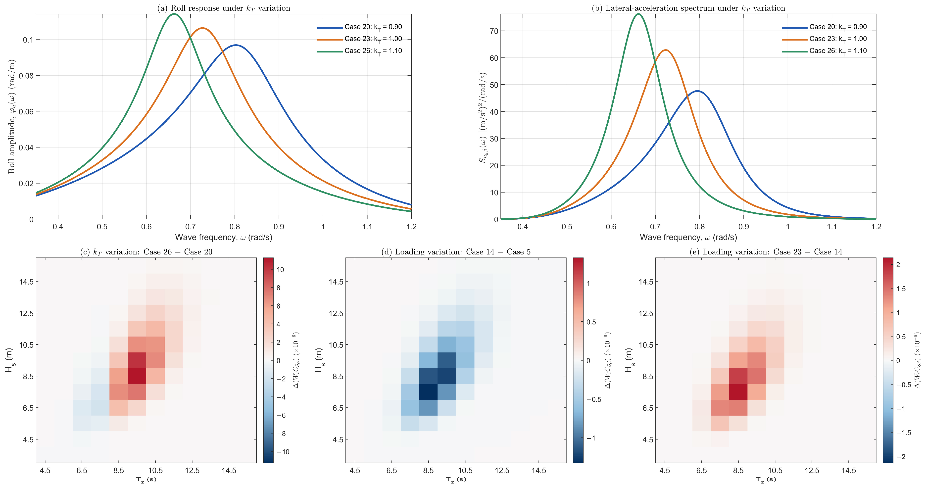
To further examine the mechanisms underlying these level-dependent responses, DTC Cases 20, 23, and 26 were selected, with loading and roll damping held constant while the natural roll period factor increased from 0.90 to 1.10. As shown in Figure 12a,b, the peak roll response progressively shifted toward lower frequencies (0.8021, 0.7265, and 0.6635 rad/s), accompanied by a corresponding redistribution of the lateral-acceleration spectral density. Despite a non-monotonic variation in EA1 lateral acceleration (9.737, 9.783, and 9.302 m/s2), the EA2 long-term probability index increased successively from 1.6590 × 10⁻⁴ to 2.3770 × 10⁻⁴ and 2.6683 × 10⁻⁴. The sea-state contribution differences in Figure 12c identify the largest positive contribution at Hs = 8.5 m and Tz = 9.5 s, whereas certain shorter-period sea states exhibit reduced contributions. This redistribution demonstrates how the interaction between frequency-dependent ship response and wave energy affects the long-term EA2 index, even when the simplified EA1 response follows a different trend.
As damping increases, both the EA1 lateral acceleration ay and the EA2 long-term probability index C decrease monotonically. In this respect, damping exhibits the highest directional consistency between the two assessment levels. However, the ships do not respond to damping variations with the same intensity. The slopes of the response curves differ noticeably, particularly in EA2, where KCS shows a much steeper damping-related variation, while ITTC A1 and DTC remain at lower and comparatively similar sensitivity levels. This indicates that the influence of kB should be interpreted in conjunction with hull geometry, hydrostatic characteristics, and the baseline roll dynamics of each ship. When the loading-condition variation in Figure 9 is considered, EA1 exhibits a directionally consistent response across the three ships, although the magnitude of this response remains ship-dependent. In contrast, the influence of loading condition on EA2 does not appear to follow a common trend. This behavior may be attributed to the fact that loading condition does not represent a single physical variable; rather, the observed ship-specific response results from the simultaneous variation in several hydrostatic and geometric quantities. These include displacement, draft, hydrostatic stiffness, and VCA from the roll axis. Since VCG and LCG were held fixed, the loading-dependent responses reflect changes in submerged hull geometry and hydrostatic properties without accounting for additional effects arising from the redistribution of onboard weights. Consequently, the observed loading sensitivity applies to the prescribed displacement variations and may differ from that of actual loading changes accompanied by shifts in the centers of gravity. One of the most important cross-level findings is therefore that kT produces opposite directional sensitivity in EA1 and EA2, kB exhibits the same directional sensitivity at both levels, whereas loading condition results in a ship-dependent cross-level response.
The non-monotonic influence of loading on DTC was investigated separately using Cases 5, 14, and 23, with both the natural roll period and damping factors fixed at 1.00. Increasing the displacement from 80% to 90% of the full-load value reduced C from 2.31565 × 10⁻⁴ to 2.16332 × 10⁻⁴ (−6.58%), whereas a further increase to full load raised it to 2.37700 × 10⁻⁴ (+9.88%). In contrast, EA1 lateral acceleration decreased continuously across these conditions. For the representative sea state Hs = 8.5 m and Tz = 8.5 s, the corresponding standard deviations of lateral acceleration exhibited a similar reversal (3.514, 3.487, and 3.529 m/s2). The contribution maps in Figure 12d,e further show that the weighted short-term failure contributions decreased from Case 5 to Case 14 and increased from Case 14 to Case 23 across the contributing sea states. This behavior indicates that the loading-dependent EA2 response cannot be characterized by displacement alone, but arises from the combined effects of changes in hydrostatic and geometric characteristics, the frequency-weighted acceleration response, and the nonlinear exceedance probability. The C values for all three conditions nevertheless remained below the EA2 acceptance threshold.
Figure 12.
Frequency-dependent roll response, lateral-acceleration spectra, and individual sea-state contribution changes for representative DTC cases. (a) Roll-response amplitude under natural roll period variation (Cases 20, 23, and 26); (b) lateral-acceleration spectral density for Hs = 8.5 m and Tz = 8.5 s under the same variations; (c) change in weighted sea-state contributions between Cases 26 and 20; (d) corresponding changes between Cases 14 and 5; and (e) between Cases 23 and 14 under successive loading variations. The contribution differences are expressed as ∆(WiCs,i), with positive values indicating increased contributions to C. Color scales are adjusted independently for each panel. The contribution maps display the principal contributing sea-state region, whereas the full sea-state grid is retained in calculating C.
Although all three benchmark vessels are container ships, their geometric proportions, hull forms, and reference stability characteristics differ considerably. For example, ITTC A1 has a higher beam-to-length ratio (0.181) than KCS (0.140) and DTC (0.144), while differences are also present in sectional geometry, bilge-keel proportions, and reference GM values (Table 1). These characteristics influence the EA assessment through several interconnected mechanisms, including wave-induced roll excitation, hydrostatic restoring properties, roll damping, and the position of the onboard acceleration assessment point relative to the roll axis. Furthermore, the hydrostatic changes associated with displacement variation are not identical among the three hulls, contributing to their different loading-dependent responses. The higher EA1 lateral accelerations observed for DTC and the greater EA2 probability indices obtained for KCS illustrate that the relative severity of excessive acceleration does not follow a common ordering across the two assessment levels. Consequently, the observed ship-dependent sensitivity reflects the combined influence of geometric and dynamic characteristics, and the individual contribution of vessel size cannot be isolated from the present comparisons.
Following the isolated-factor assessment presented in Figure 9, Figure 10 and Figure 11 extend the analysis to the combined variation in two parameters while the remaining factor is held at its reference value. The EA1 response surfaces in Figure 10 are generally smooth and approximately planar for all three ships, with no pronounced curvature or abrupt changes across the kT × kB, kT × ∇, and kB × ∇ combinations. This behavior suggests that, within the investigated ranges, the EA1 response is governed predominantly by the main effects, while two-factor interactions remain comparatively limited. In the kT × kB plane, lateral acceleration decreases systematically as both factors increase, with the highest ay values occurring at low kT and low kB. Moreover, the ship-wise ordering remains largely unchanged throughout the two-factor space, with ITTC A1 exhibiting the lowest, KCS intermediate, and DTC the highest lateral acceleration levels. A different response structure emerges in Figure 11 for EA2, where the surfaces are presented on a logarithmic C-axis to accommodate the substantial differences in the long-term probability index. KCS exhibits noticeably steeper surfaces and a broader response range than the other two ships, confirming that its strong sensitivity observed in the isolated-factor analysis persists under combined parameter variations. A particularly elevated C region is also evident for KCS in the kT × ∇ surface, indicating that certain combinations of these factors can substantially amplify its EA2 response. In contrast, although DTC consistently produces the highest EA1 lateral accelerations, it does not generate the highest EA2 probability surfaces, further demonstrating that the relative severity observed at Level 1 is not directly preserved at Level 2. Overall, the smoother and more nearly additive EA1 surfaces contrast with the stronger slope variations and ship-dependent geometry observed in EA2, providing a visual indication of greater interaction sensitivity at Level 2 and a useful basis for interpreting the variance-decomposition results in Table 4 and Table 5.
The variance decomposition in Table 4 and Table 5 indicates that the transition from EA1 to EA2 involves more than a simple redistribution of parameter importance; it reflects a change in the mechanisms governing the calculated response. In EA1, the natural roll period factor kT provides the largest pooled contribution (41.134%), which is consistent with the direct role of Tr in the Level 1 lateral-acceleration formulation and in the estimation of the characteristic roll amplitude. This dominance is particularly strong for ITTC A1 and KCS, whereas DTC departs from this pattern, with loading condition becoming the principal source of variation. In EA2, however, roll damping becomes the dominant pooled contributor (43.009%), followed by loading condition (34.789%), while the contribution of kT decreases markedly to 14.956%. This shift is physically significant because EA2 evaluates the response through a frequency-dependent roll model and a probabilistically weighted long-term formulation, in which damping directly controls the amplification of roll response in the vicinity of resonance. The exceptionally large damping contribution for DTC (84.518%) therefore suggests that its EA2 vulnerability is governed predominantly by the suppression or amplification of resonant roll response rather than by period variation alone. KCS exhibits a different balance, with loading and damping contributing almost equally, indicating a more coupled sensitivity to hydrostatic state and roll-response characteristics. Moreover, the combined interaction contribution increases from approximately 2.1% in EA1 to 7.2% in EA2. Although main effects remain dominant, this increase confirms that the more detailed Level 2 formulation is more sensitive to the simultaneous variation in the investigated parameters. Thus, the decomposition reveals a clear cross-level shift from a primarily period-controlled EA1 response toward a more damping- and loading-controlled EA2 response, with the extent of this shift remaining strongly ship-specific.
The large EA2 damping contribution, particularly the 84.518% obtained for DTC, should be interpreted within the Simplified Ikeda-based damping model and the prescribed parameter variation ranges. This percentage represents the relative contribution of roll damping to the computed response variance, rather than a model-independent measure of its influence. Since the reference damping was estimated at a fixed roll amplitude of 15°, alternative damping predictions or experimentally derived damping coefficients could lead to different EA2 probability indices and sensitivity contributions. Such alternatives were not examined in the present study.
Table 6 condenses these differences into their directional safety consequences and therefore provides a useful synthesis of the cross-level behavior. Increasing kB is the only variation that produces a consistently favorable response for all three ships at both levels, reinforcing the stabilizing role of increased roll damping within the excessive-acceleration assessment. By contrast, increasing kT generally improves the normalized EA1 response while worsening EA2, with DTC showing a non-monotonic but overall improving EA1 trend. Loading condition exhibits a similarly divergent pattern: increased loading improves EA1 for all three ships, whereas the corresponding EA2 response worsens for ITTC A1 and KCS and becomes non-monotonic, with an overall worsening tendency, for DTC. This directional inconsistency is important because it shows that parameter variations that appear beneficial under the simplified Level 1 formulation cannot automatically be interpreted as beneficial when the frequency-dependent and probabilistic treatment of Level 2 is considered. Table A5, Table A6 and Table A7 in Appendix C complement this interpretation by providing the complete case-wise normalized responses, safety margins, and threshold classifications from which these aggregate tendencies are obtained. They also preserve traceability between individual factor combinations and the resulting EA1 and EA2 classifications. Taken together, the variance decomposition, directional summary, and case-level results establish that SGISC excessive acceleration sensitivity is not governed by a single universal parameter hierarchy; rather, it emerges from the combined effects of assessment level, ship-specific dynamics, and the way each variation enters the underlying response formulation.
6. Conclusions
This study examined the sensitivity and cross-level consistency of the SGISC excessive acceleration assessment under variations in natural roll period, roll damping, and loading condition for three benchmark container ships. Of the 72 cases within the IMO applicability range, all failed EA1, whereas 50 passed EA2 and 22 failed at both levels. The remaining nine ITTC A1 cases were retained in the numerical sensitivity analyses but excluded from these applicability-based statistics. Since none of the applicable cases passed EA1, the possibility of an EA1 PASS–EA2 FAIL outcome could not be evaluated, limiting conclusions regarding categorical cross-level consistency. Nevertheless, the systematic comparison of parameter-induced responses at both assessment levels provides a quantitative basis for investigating trend-based cross-level consistency, including the identification of consistent and level-dependent response trends. The investigated parameters produced clearly different cross-level responses. Increasing the natural roll period generally reduced EA1 lateral acceleration while increasing the EA2 long-term probability index, whereas increasing roll damping consistently reduced both responses. Loading condition exhibited a more ship-dependent behavior, particularly at Level 2. The variance-decomposition results further showed that the dominant source of variation changes between the two assessment levels: natural roll period had the largest pooled contribution in EA1, while roll damping became dominant in EA2, followed by loading condition. Interaction effects remained secondary to the main effects but were more evident in EA2, reflecting the greater sensitivity of the Level 2 formulation to combined parameter variations. The results therefore indicate that trends inferred from EA1 cannot be transferred directly to EA2 and that excessive acceleration sensitivity depends strongly on both assessment level and ship-specific characteristics.
The present study has two limitations that should be considered when interpreting its findings. First, the relatively high reference GM values adopted for ITTC A1 (6.000 m), KCS (7.705 m), and DTC (12.918 m) were established for a controlled EA sensitivity investigation and do not represent the full range of stability conditions encountered in service. Second, the variations in natural roll period and roll damping were restricted to a relatively narrow range (kT and kB = 0.90–1.10). Consequently, the identified sensitivity trends and cross-level relationships should not be assumed to remain unchanged under substantially different reference stability conditions or broader parameter variations.
Future work should extend the analysis to additional ship types and wider operational conditions. More realistic loading variations incorporating changes in weight distribution, centers of gravity, and related hydrostatic properties should also be considered. Further investigation of alternative damping models, environmental spectra, and higher-fidelity numerical or experimental approaches would help assess the robustness and broader applicability of the cross-level relationships identified here.
Author Contributions
Conceptualization, F.T.K.; methodology, F.T.K. and H.A.; software, F.T.K.; validation, F.T.K. and H.A.; formal analysis, F.T.K. and H.A.; investigation, F.T.K.; writing—original draft preparation, F.T.K.; writing—review and editing, F.T.K. and H.A.; visualization, F.T.K.; supervision, H.A. All authors have read and agreed to the published version of the manuscript.
Funding
This research received no external funding.
Data Availability Statement
The data supporting the findings of this study are available within the article and its Appendices. Additional data are available from the corresponding author upon reasonable request.
Conflicts of Interest
The authors declare no conflicts of interest.
Abbreviations
The following abbreviations are used in this manuscript:
| IMO | International Maritime Organization |
| SGISC | Second-generation intact stability criteria |
| EA | Excessive acceleration |
| PR | Parametric rolling |
| DS | Dead ship condition |
| PL | Pure loss of stability |
| SR | Surf-riding/broaching |
| EA1 | Excessive acceleration Level 1 |
| EA2 | Excessive acceleration Level 2 |
| GM | Metacentric height |
| VCG | Vertical Center of Gravity |
| LCG | Longitudinal Center of Gravity |
| VCA | Vertical Center of Acceleration |
| LCA | Longitudinal Center of Acceleration |
| ANOVA | Analysis of Variance |
| SS | Sum of Squares |
List of Symbols
The following symbols are used in this manuscript:
| KG | Height of the center of gravity above the keel | m |
| Hs | Significant wave height | m |
| Tz | Mean zero-crossing wave period | s |
| g | Gravitational acceleration | m/s2 |
| GM | Metacentric height | m |
| B | Ship breadth | m |
| h | Height of the acceleration assessment location | m |
| d | Mean draught | m |
| C | Long-term probability index in EA2 | – |
| Tr | Natural roll period | s |
| kT | Natural roll period variation factor | – |
| c (Equation (1)) | Empirical coefficient for natural roll period estimation | – |
| LWL | Waterline length | m |
| Tr,var | Modified natural roll period | s |
| δφ | Logarithmic decrement of roll decay | – |
| B44 | Equivalent linear roll damping coefficient | N·m·s |
| kB | Roll damping variation factor | – |
| δφ,var | Modified logarithmic decrement of roll decay | – |
| RPR | Roll damping parameter used in EA1 | – |
| B44,var | Modified equivalent linear roll damping coefficient | N·m·s |
| lbk | Bilge keel length | m |
| hbk | Bilge keel height | m |
| LBP | Length between perpendiculars | m |
| KM | Height of the transverse metacenter above the keel | m |
| hk | Vertical height of the acceleration assessment location above the keel | m |
| D | Molded depth | m |
| x | Longitudinal position of the acceleration assessment location | m |
| L | Ship length | m |
| ay | Lateral acceleration | m/s2 |
| yijk | Calculated response for a specified combination of the three factors | variable |
| i,j,k | Indices of loading condition, natural roll period factor, and roll damping factor | – |
| Overall mean response | variable | |
| Mean response at loading condition level i | variable | |
| Mean response at natural roll period factor level j | variable | |
| Mean response at roll damping factor level k | variable | |
| Mean response for the loading–period factor combination | variable | |
| Mean response for the loading–damping factor combination | variable | |
| Mean response for the period–damping factor combination | variable | |
| SSL,SST,SSB | Main-effect sums of squares | variable2 |
| SSLT,SSLB,SSTB | Two-factor interaction sums of squares | variable2 |
| SSTotal | Total sum of squares | variable2 |
| SSLTB | Three-factor interaction sum of squares | variable2 |
| Pm | Percentage contribution of component m to total variation | % |
| SSm | Sum of squares associated with component m | variable2 |
| kL | Longitudinal assessment position correction factor | – |
| r | Effective wave slope coefficient in EA1 | – |
| Non-dimensional breadth parameter | – | |
| Non-dimensional draught parameter | – | |
| β | Auxiliary coefficient in the EA1 effective wave slope calculation | – |
| τ | Auxiliary coefficient in the EA1 effective wave slope calculation | – |
| F | Auxiliary dimensionless term in the EA1 effective wave slope calculation | – |
| K1,K2 | Auxiliary terms in the EA1 effective wave slope calculation | m |
| s | Wave steepness | – |
| φ | Roll angle | rad |
| hr | Effective vertical distance used in the lateral acceleration calculation | m |
| Non-dimensional equivalent linear roll damping coefficient | – | |
| ω | Circular frequency | rad/s |
| r(ω) | Frequency-dependent effective wave slope coefficient | – |
| λ | Wavelength | m |
| σLA,i | Standard deviation of lateral acceleration for sea state i | m/s2 |
| Szz | Wave elevation spectral density | m2/(rad/s) |
| σLA | Standard deviation of lateral acceleration | m/s2 |
| REA2 | EA2 acceptance threshold | – |
| ωr | Natural roll frequency | rad/s |
| Frequency corresponding to maximum roll amplitude | rad/s | |
| Frequency corresponding to maximum lateral acceleration | rad/s | |
| REA1 | EA1 acceptance threshold | m/s2 |
| ∇ | Displacement volume | m3 |
| C (x) (Equation (23)) | Equivalent-section contribution function | m3 |
| ω1, ω2 | Lower and upper frequency limits | rad/s |
| ∆ω | Frequency increment | rad/s |
| ωj | Midpoint frequency of interval j | rad/s |
| Wi | Occurrence weight of sea state i | – |
| Cs,i | Short-term excessive acceleration failure index | – |
| R2 | Lateral acceleration threshold in EA2 | m/s2 |
| φa(ω) | Roll-response amplitude per unit wave amplitude | rad/m |
| ay(ω) | Lateral acceleration response per unit wave amplitude | (m/s2)/m |
| Lateral-acceleration spectral density | (m/s2)2/(rad/s) | |
| ∇eq | Equivalent underwater hull volume | m3 |
| ρ | Seawater density | kg/m3 |
| BF,BW,BE,BL,BBK | Individual roll-damping contributions | N·m·s |
| JT,roll | Total roll moment of inertia, including added inertia | t·m2 |
| φr(ω), φi(ω) | Cosine and sine roll-response components | rad/m |
Appendix A
The excessive acceleration (EA) provisions are applicable to ships and loading conditions satisfying the applicability requirements specified by IMO [1], including the limits related to the vertical location of occupied spaces and metacentric height. These conditions may be regarded as defining the intended applicability range of the EA formulation, while also identifying ship configurations for which the geometric and stability characteristics may increase susceptibility to excessive lateral accelerations. Satisfaction of these applicability conditions, however, does not by itself imply vulnerability; the vulnerability assessment is determined through the subsequent Level 1 and Level 2 criteria.
Figure A1 presents the spreadsheet in which the outputs of the in-house MATLAB code, which forms the computational basis of the calculations and figures presented in this study, were organized. The progression of the prescribed variations over the 27 cases can be followed separately for each ship. The color coding used in the kB variation columns indicates whether each case satisfies the two IMO applicability conditions [1] for the EA assessment. Red denotes cases satisfying both applicability conditions, whereas green denotes cases for which at least one of these conditions is not satisfied.
The PASS/FAIL column associated with Level 1 was assigned according to the lateral-acceleration criterion. Cases exceeding the critical lateral-acceleration threshold were classified as FAIL and highlighted in red, whereas cases below the threshold were classified as PASS and highlighted in green. The same visual convention was applied to the Level 2 results: cases for which the long-term probability index C exceeded its acceptance limit were classified as FAIL and shown in red, while the remaining cases were classified as PASS and shown in green.
Figure A1.
Complete case design and corresponding EA1 and EA2 results for ITTC A1, KCS, and DTC.
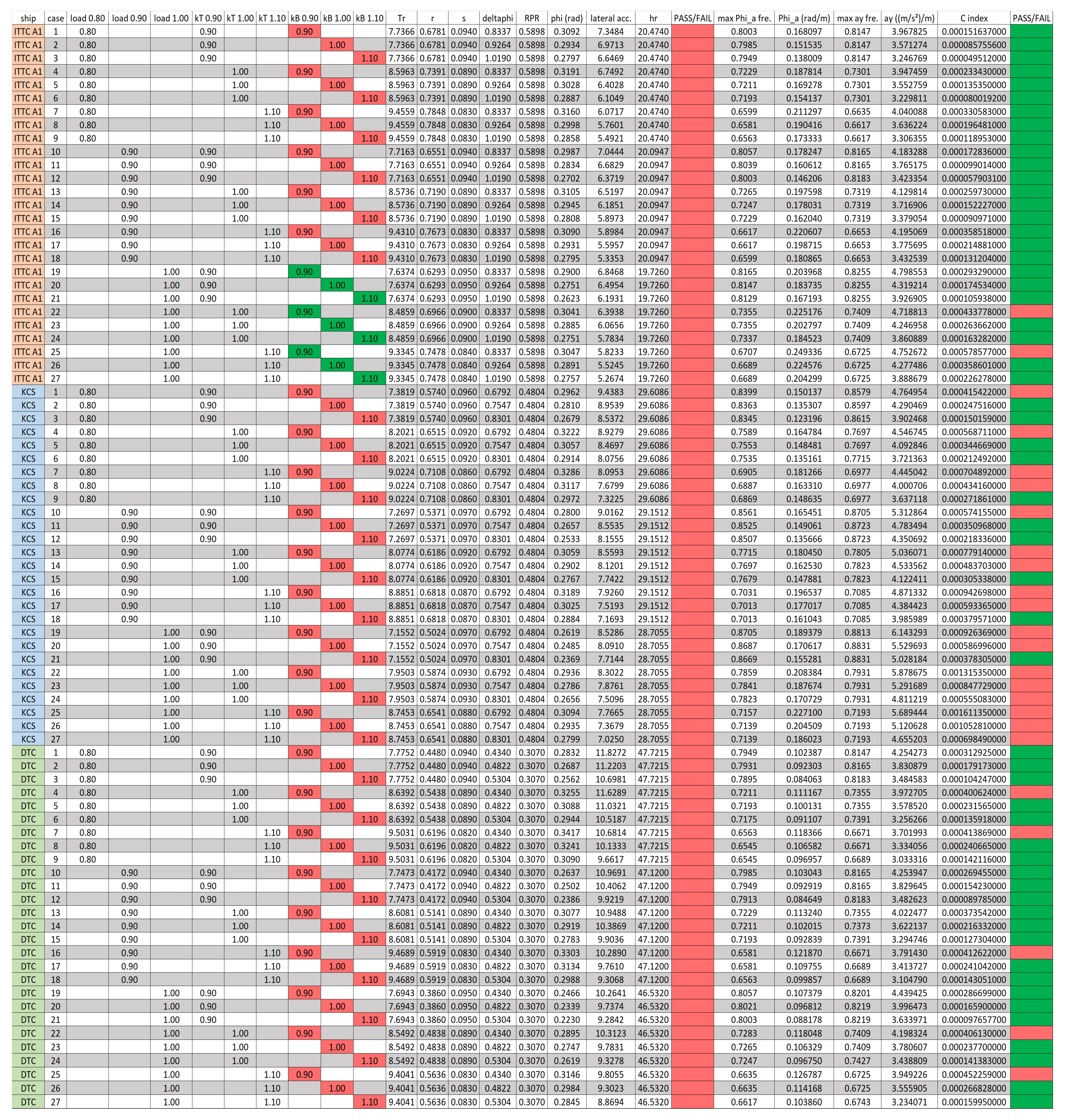
Table A1.
Displacement volume, equilibrium draught, KM, VCG, and GM for the investigated loading conditions of ITTC A1, KCS, and DTC.
Appendix B
Appendix B presents the validation of the in-house MATLAB code by comparison with the corresponding IMO results for the C11 example ship. Three tables are provided: the IMO values for the standard deviation of lateral acceleration, σLAi, the corresponding values calculated using the in-house MATLAB code, and percentage differences between the two datasets.
Table A2.
Standard deviation of lateral acceleration values, σLA,i, of the IMO example.
Table A3.
Standard deviation of lateral acceleration values, σLA,i, of the in-house MATLAB code.
Table A4.
Percentage differences in the standard deviation of lateral acceleration, σLA,i, between the in-house MATLAB results and the corresponding IMO values.
Appendix C
Appendix C presents the complete 27-case datasets for ITTC A1, KCS, and DTC in Table A5, Table A6 and Table A7, respectively. For each case, the prescribed loading condition, natural roll period factor kT, and roll damping factor kB are listed together with the normalized EA1 lateral acceleration ay/REA1, the corresponding Level 1 safety margin and classification, the normalized EA2 long-term probability index C/REA2, and the corresponding Level 2 safety margin and classification. The tables therefore provide the case-by-case numerical values underlying the Level 1 and Level 2 comparisons discussed in the main text.
Table A5.
Case-wise normalized EA1 and EA2 vulnerability measures, safety margins, and threshold-based classifications for ITTC A1.
Table A6.
Case-wise normalized EA1 and EA2 vulnerability measures, safety margins, and threshold-based classifications for KCS.
Table A7.
Case-wise normalized EA1 and EA2 vulnerability measures, safety margins, and threshold-based classifications for DTC.
References
- International Maritime Organization (IMO). Interim Guidelines on the Second-Generation Intact Stability Criteria; MSC.1/Circ.1627; International Maritime Organization (IMO): London, UK, 2020. [Google Scholar]
- Tadros, M.; Aung, M.Z.; Louvros, P.; Pollalis, C.; Nazemian, A.; Boulougouris, E. Ship manoeuvring research 2010–2025: From hydrodynamics and control to digital twins, AI and MASS. J. Mar. Sci. Eng. 2025, 13, 2322. [Google Scholar] [CrossRef] [Scilit]
- Somayajula, A.; Falzarano, J.; Lutes, L. An efficient assessment of vulnerability of a ship to parametric roll in irregular seas using first passage statistics. Probab. Eng. Mech. 2019, 58, 102998. [Google Scholar] [CrossRef] [Scilit]
- Chung, J.; Shin, D.M.; Kim, W.D.; Moon, B.Y. Current status of the 2nd generation of intact stability: Investigation of the pure loss of stability and parametric roll mode. J. Ocean Eng. Technol. 2020, 34, 55–65. [Google Scholar] [CrossRef] [Scilit]
- International Maritime Organization (IMO). Explanatory Notes to the Interim Guidelines on the Second-Generation Intact Stability Criteria; MSC.1/Circ.1652; International Maritime Organization (IMO): London, UK, 2023. [Google Scholar]
- Boccadamo, G.; Rosano, G. Excessive acceleration criterion: Application to naval ships. J. Mar. Sci. Eng. 2019, 7, 431. [Google Scholar] [CrossRef] [Scilit]
- Shin, D.-M.; Moon, B.-Y. Assessment of excessive acceleration of the IMO second generation intact stability criteria for the tanker. J. Mar. Sci. Eng. 2022, 10, 229. [Google Scholar] [CrossRef] [Scilit]
- Marlantes, K.E.; Kim, S.; Hurt, L.A. Implementation of the IMO second generation intact stability guidelines. J. Mar. Sci. Eng. 2022, 10, 41. [Google Scholar] [CrossRef] [Scilit]
- Begović, E.; Boccadamo, G.; Rinauro, B.; Rosano, G. Excessive acceleration simplified operational guidance. Int. J. Nav. Archit. Ocean Eng. 2022, 14, 100473. [Google Scholar] [CrossRef] [Scilit]
- Duan, F.; Ma, N.; Gu, X.C.; Zhou, Y.H.; Wang, S.M. A fast time domain method for predicting of motion and excessive acceleration of a shallow draft ship in beam waves. Ocean Eng. 2022, 262, 112096. [Google Scholar] [CrossRef] [Scilit]
- Rosano, G.; Begović, E.; Boccadamo, G.; González, M.M.; Rinauro, B.; Caamaño, L.S. On-board monitoring and estimation of lateral accelerations through extreme value theory. Ocean Eng. 2023, 284, 115177. [Google Scholar] [CrossRef] [Scilit]
- Paroka, D.; Muhammad, A.H.; Rachman, S. Vulnerability assessment for excessive acceleration failure mode of an Indonesian Ro-Ro ferry by model experiment. Int. J. Technol. 2025, 16, 72–81. [Google Scholar] [CrossRef] [Scilit]
- Kuroda, T. Study of parameters for excessive acceleration failure mode in design stage. Ocean Eng. 2026, 350, 124250. [Google Scholar] [CrossRef] [Scilit]
- Kuroda, T. Evaluation and countermeasure for excessive acceleration at the bridge caused by the ship stability. In Proceedings of the 15th International Symposium on Practical Design of Ships and Other Floating Structures (PRADS 2022), Dubrovnik, Croatia, 9–13 October 2022. [Google Scholar]
- Jiang, C.; Xiang, X.; Xiang, G. A joint multi-model machine learning prediction approach based on confidence for ship stability. Complex Intell. Syst. 2024, 10, 3873–3890. [Google Scholar] [CrossRef] [Scilit]
- Qi, J.; Chai, W.; Wu, J.; Cui, M.; Cai, B.; Zhou, L. Roll motion characteristics of a polar research ship with ice accumulation in beam waves. Int. J. Nav. Archit. Ocean Eng. 2025, 17, 100678. [Google Scholar] [CrossRef] [Scilit]
- Schrøter, C.; Lützen, M.; Erichsen, H.; Jensen, J.J.; Kristensen, H.O.; Lauridsen, P.H.; Tunccan, O.; Baltsersen, J.P. Second generation intact stability criteria—Robustness and consistency analysis. In Contemporary Ideas on Ship Stability: From Dynamics to Criteria; Spyrou, K.J., Belenky, V.L., Katayama, T., Bačkalov, I., Francescutto, A., Eds.; Springer: Cham, Switzerland, 2023; Volume 134, pp. 59–71. [Google Scholar] [CrossRef] [Scilit]
- Petacco, N.; Ruggiero, V.; Gualeni, P. An investigation about stability in waves of large pleasure yachts. J. Mar. Sci. Eng. 2023, 11, 2039. [Google Scholar] [CrossRef] [Scilit]
- Yang, K.-K. Parameter sensitivity of the excessive acceleration failure mode in second-generation intact stability. Proc. Inst. Mech. Eng. Part M J. Eng. Marit. Environ. 2023, 237, 906–917. [Google Scholar] [CrossRef] [Scilit]
- Duan, F.; Ma, N.; Shi, Q.; Gu, X.; Zhou, Y. Vulnerability assessment of excessive acceleration of an offshore support vessel with moonpool. In Proceedings of the 19th International Ship Stability Workshop (ISSW 2023), Istanbul, Turkey, 11–13 September 2023; pp. 237–247. [Google Scholar]
- Montgomery, D.C. Design and Analysis of Experiments, 8th ed.; John Wiley & Sons: Hoboken, NJ, USA, 2012. [Google Scholar]
- Osaka University. ITTC A1 Container Ship: Hull Geometry and Benchmark Data. Available online: http://www.naoe.eng.osaka-u.ac.jp/imo/a1 (accessed on 25 October 2026).
- National Maritime Research Institute (NMRI). KRISO Container Ship (KCS): Geometry and Conditions. Tokyo 2015 CFD Workshop. Available online: https://www.nmri.go.jp/archives/institutes/fluid_performance_evaluation/cfd_rd/cfdws15/kcs_gc.html (accessed on 25 October 2026).
- University of Duisburg-Essen. Duisburg Test Case (DTC): CAD Files. Available online: https://www.uni-due.de/imperia/md/content/inam/igs_ordner.zip (accessed on 25 October 2026).
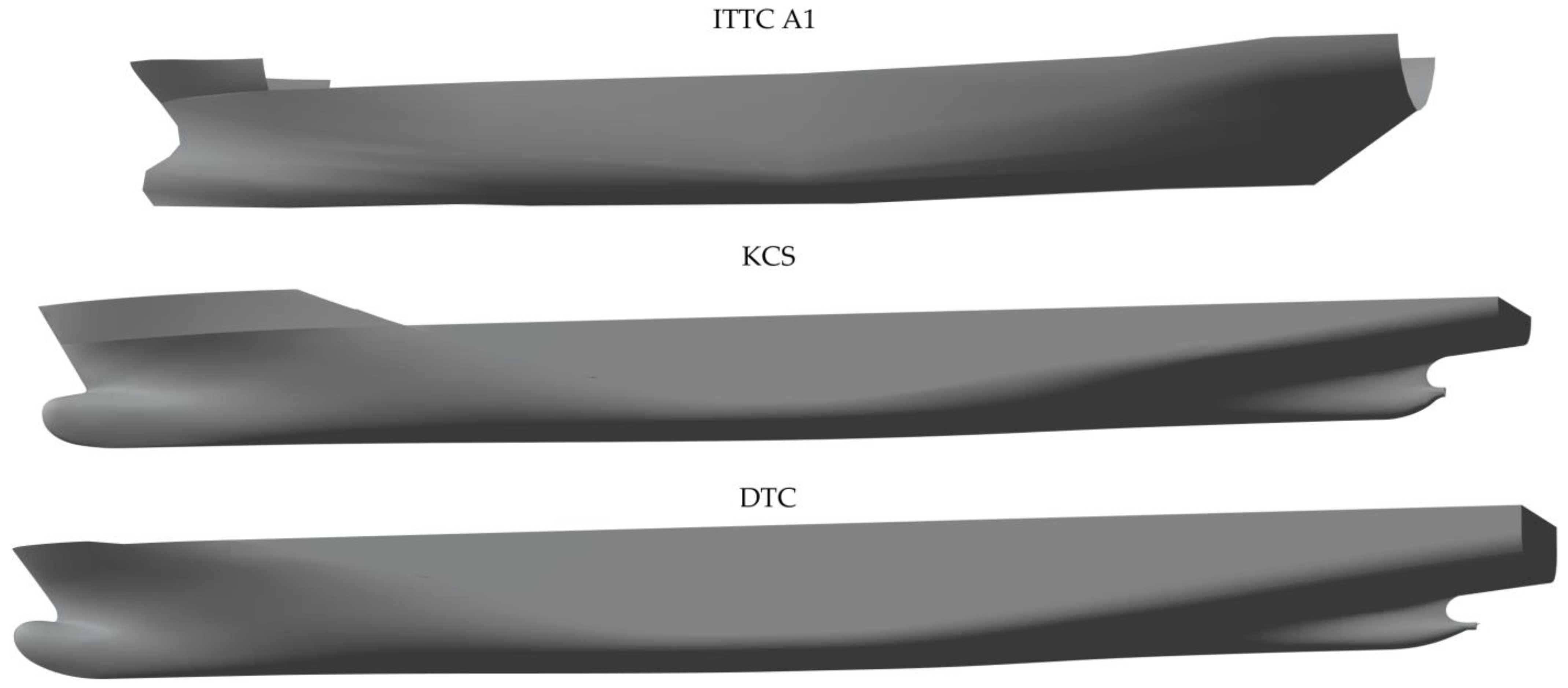
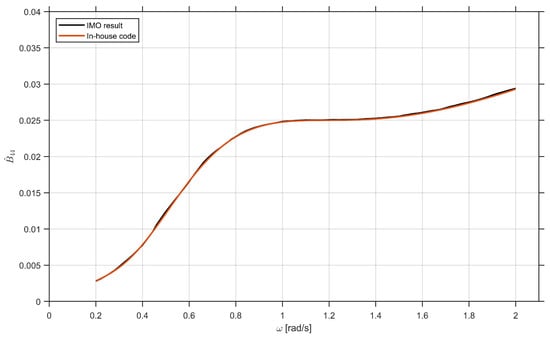
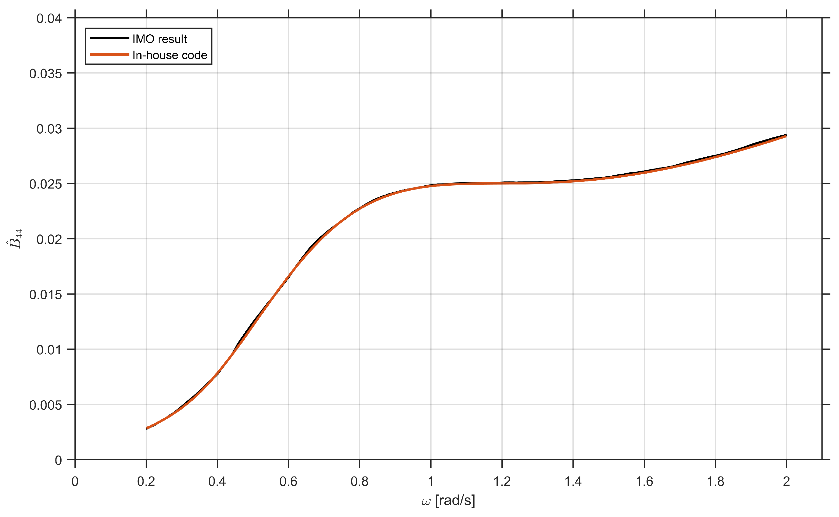
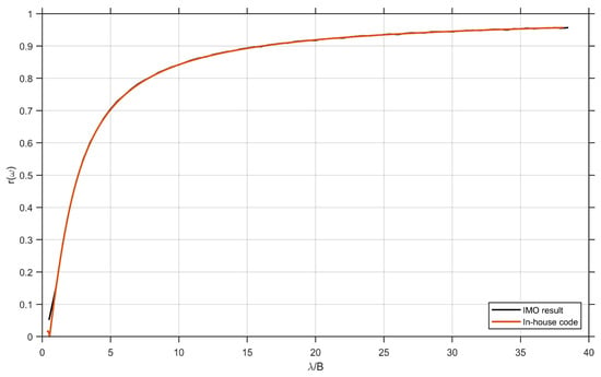
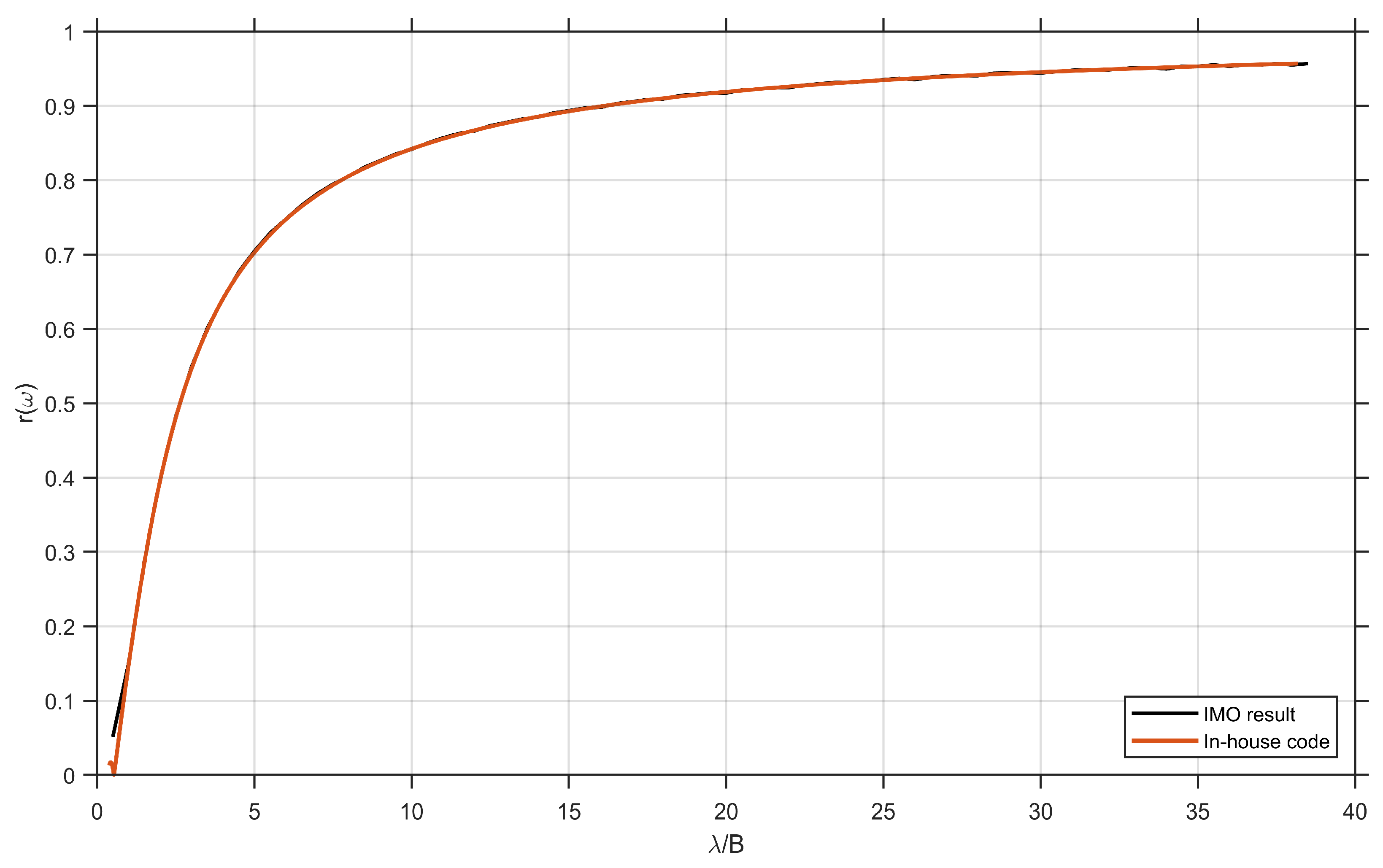
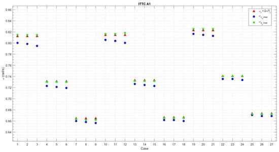
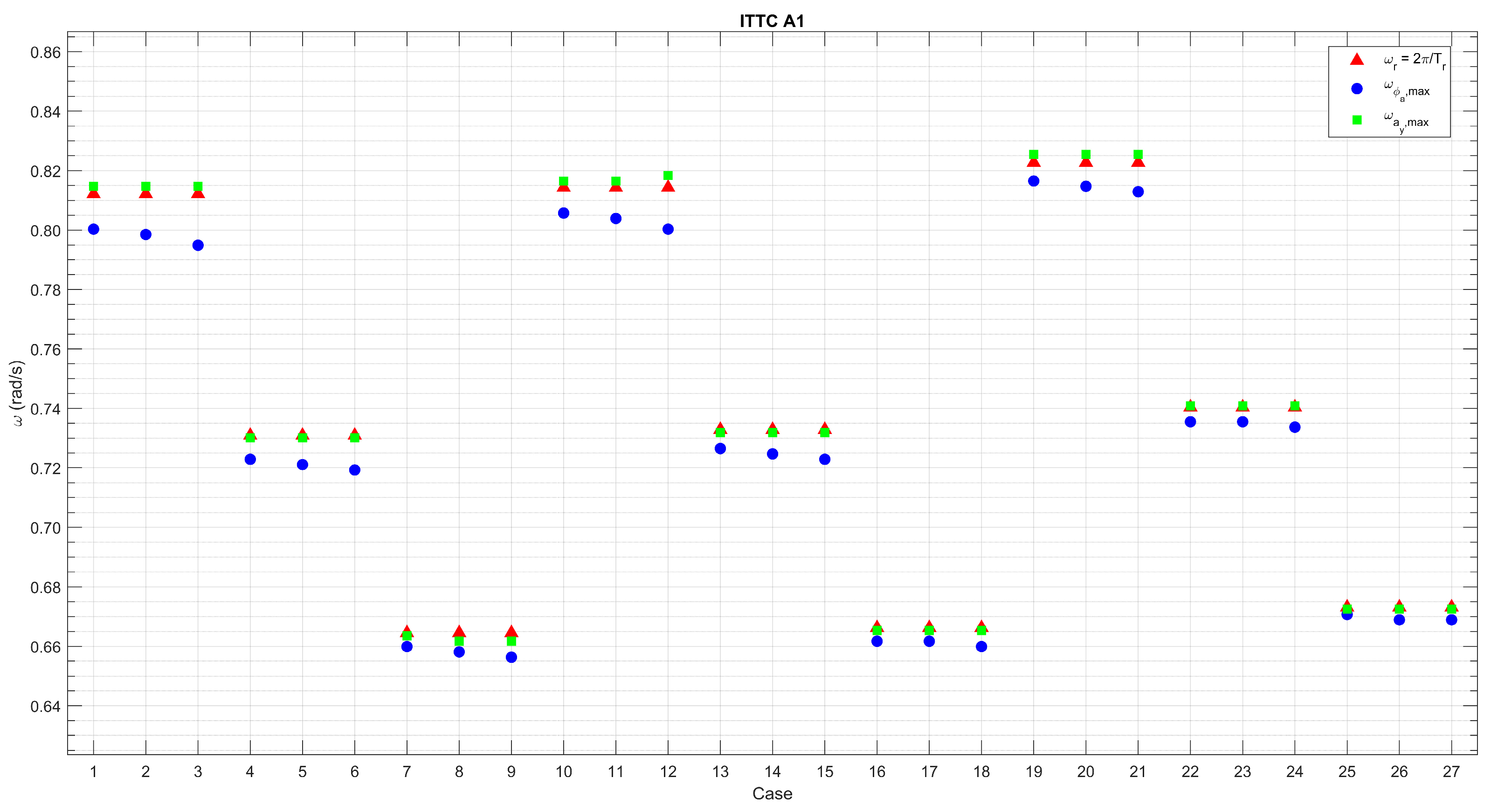
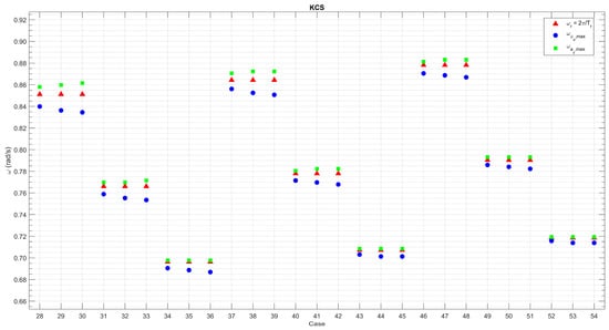
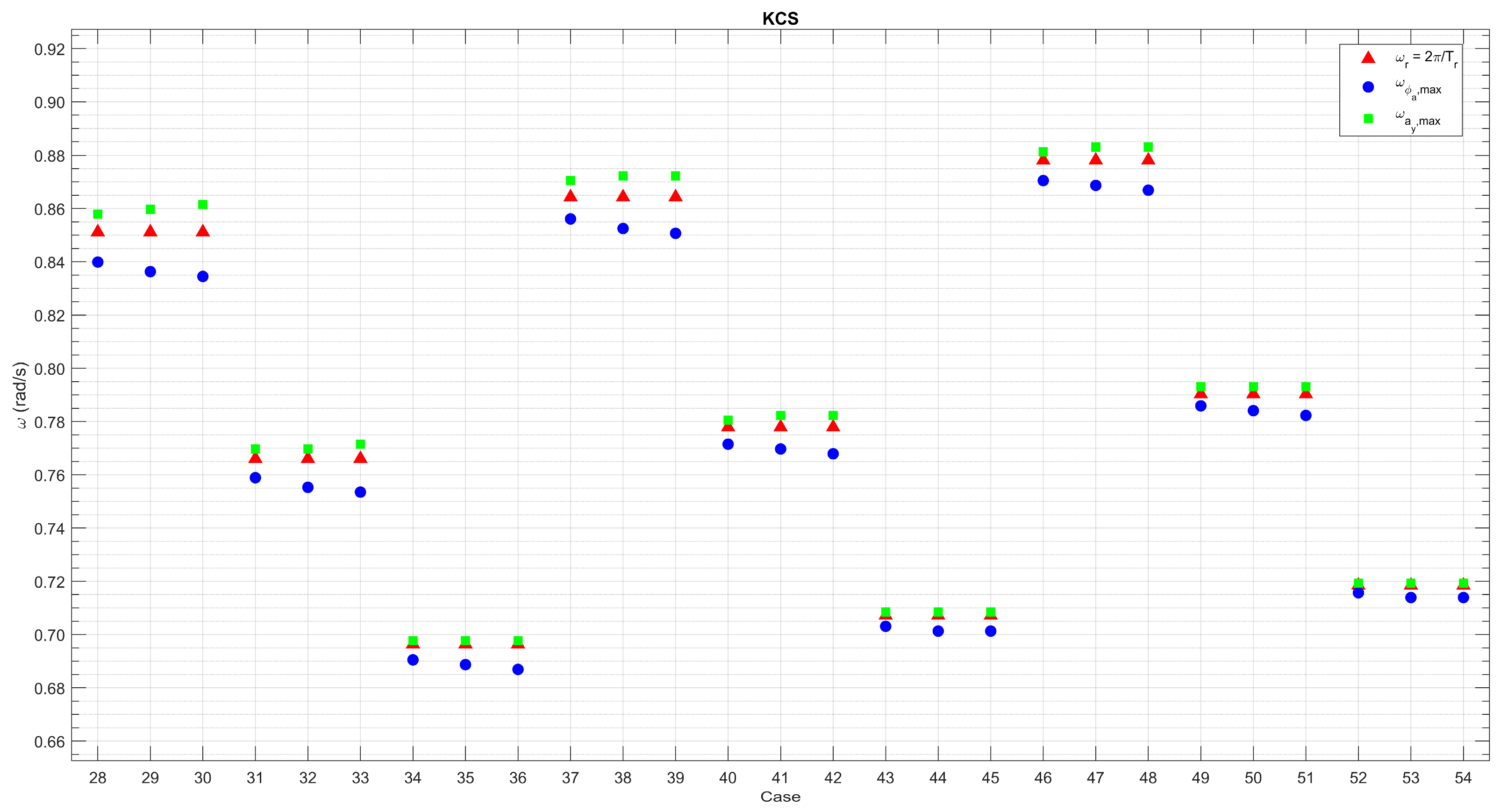
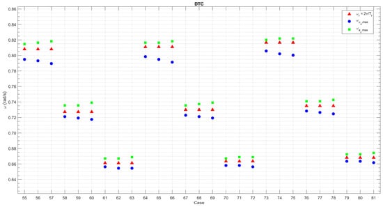
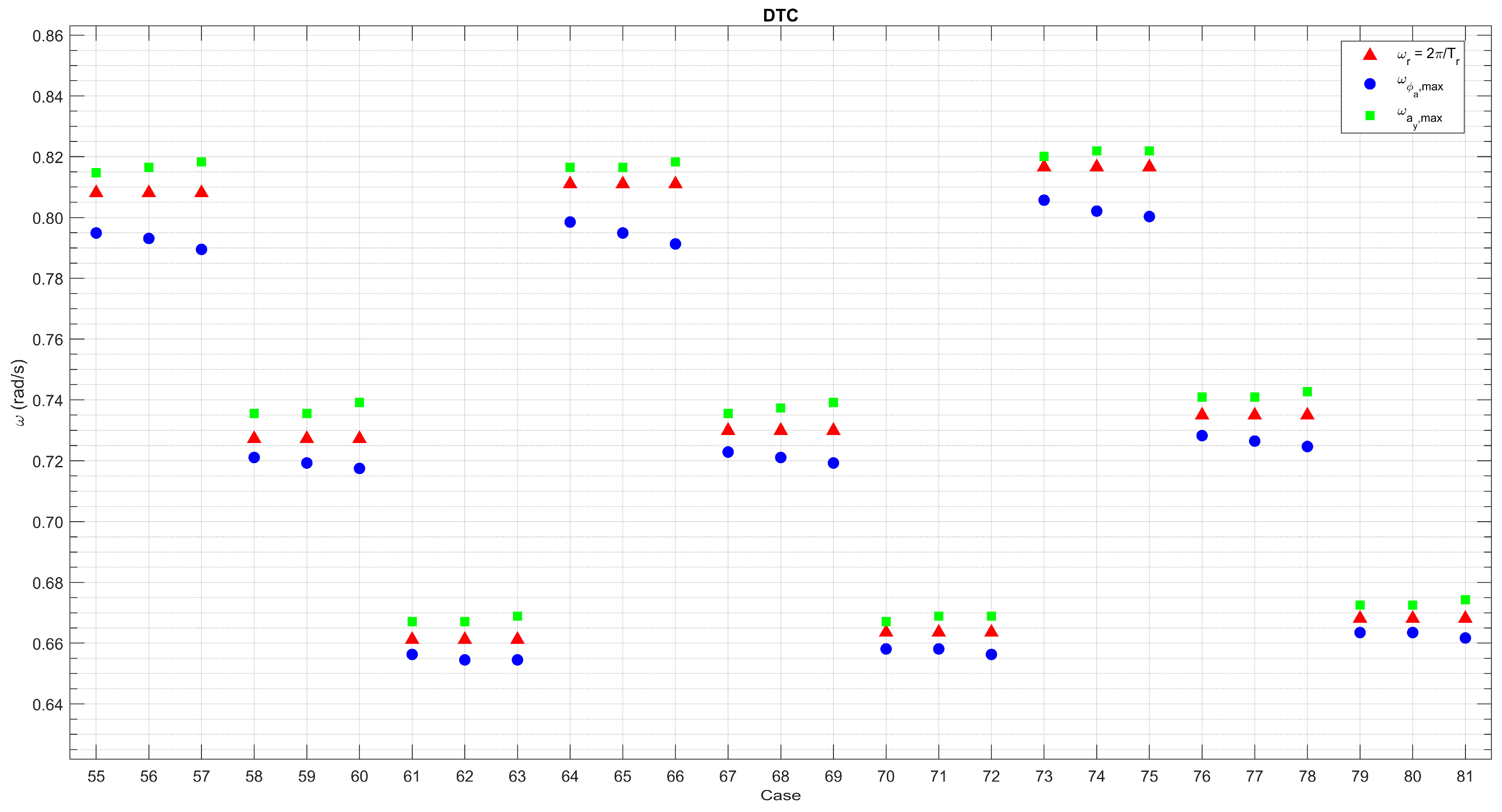
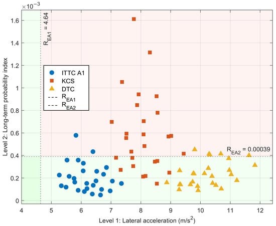
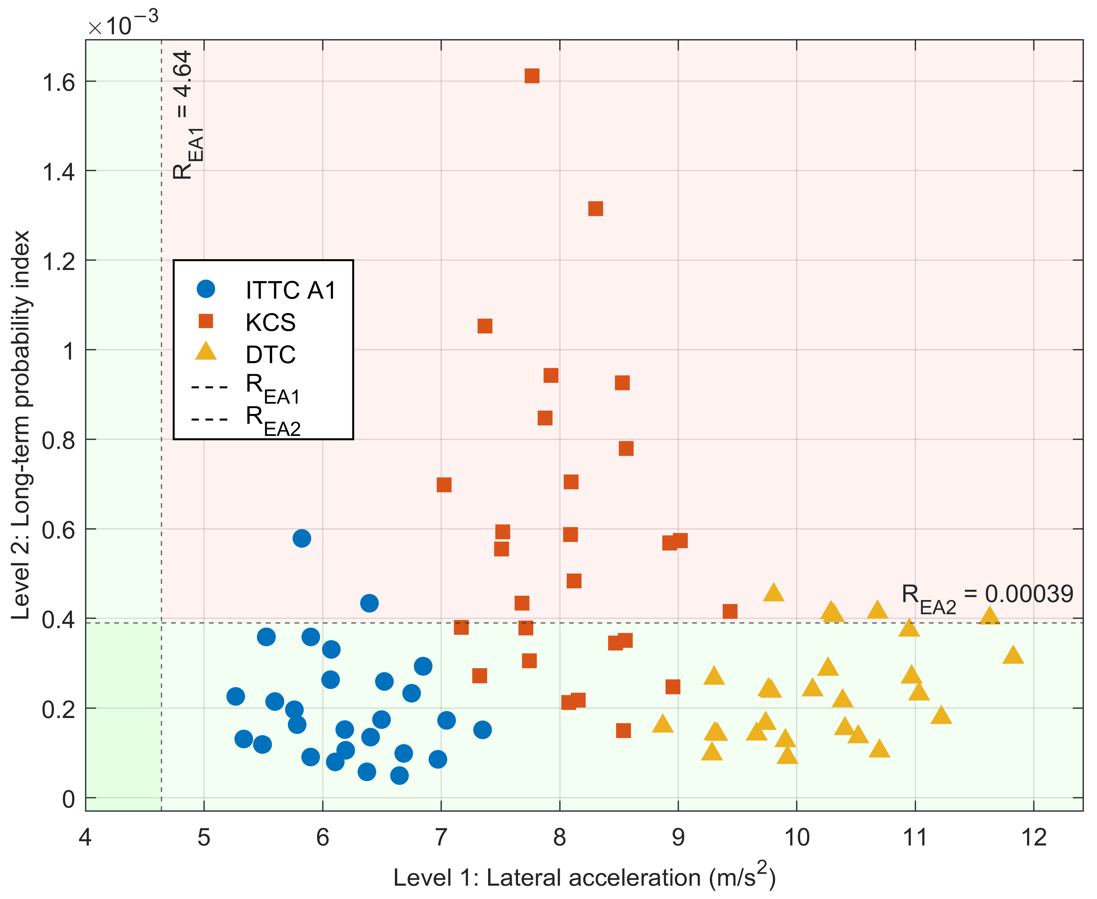
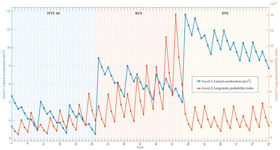
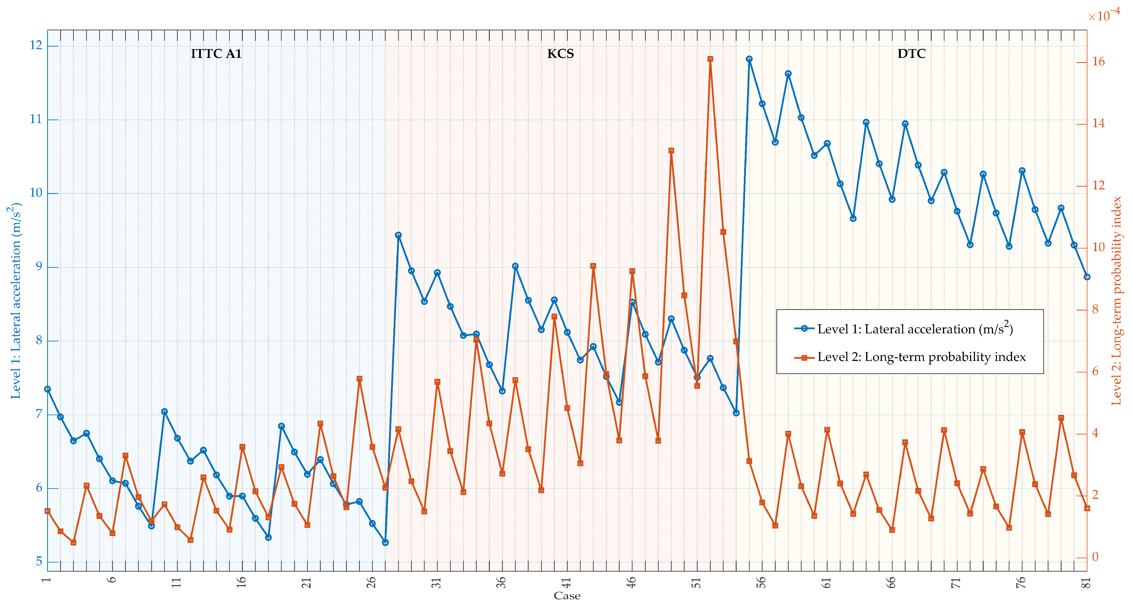
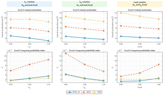
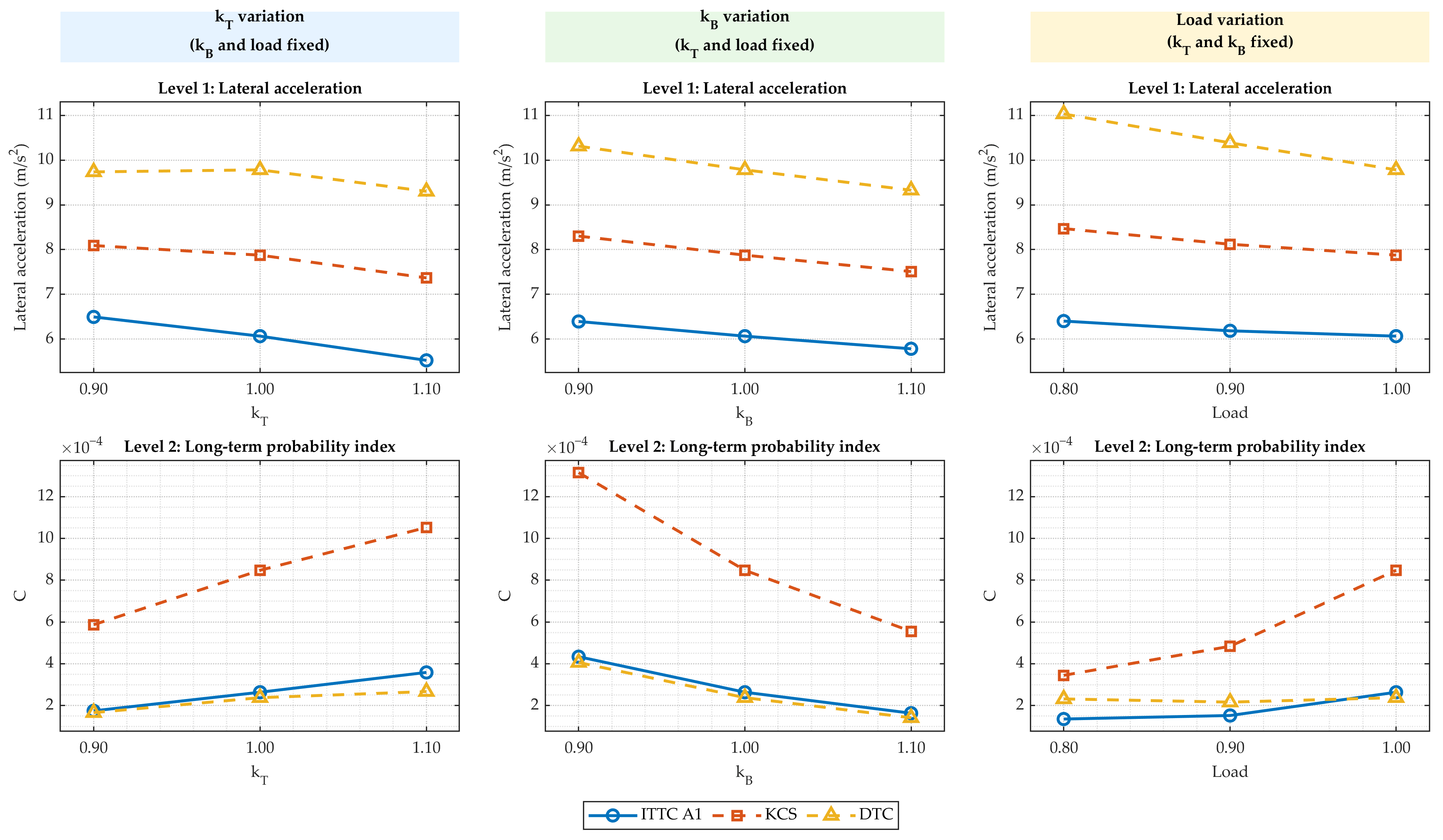
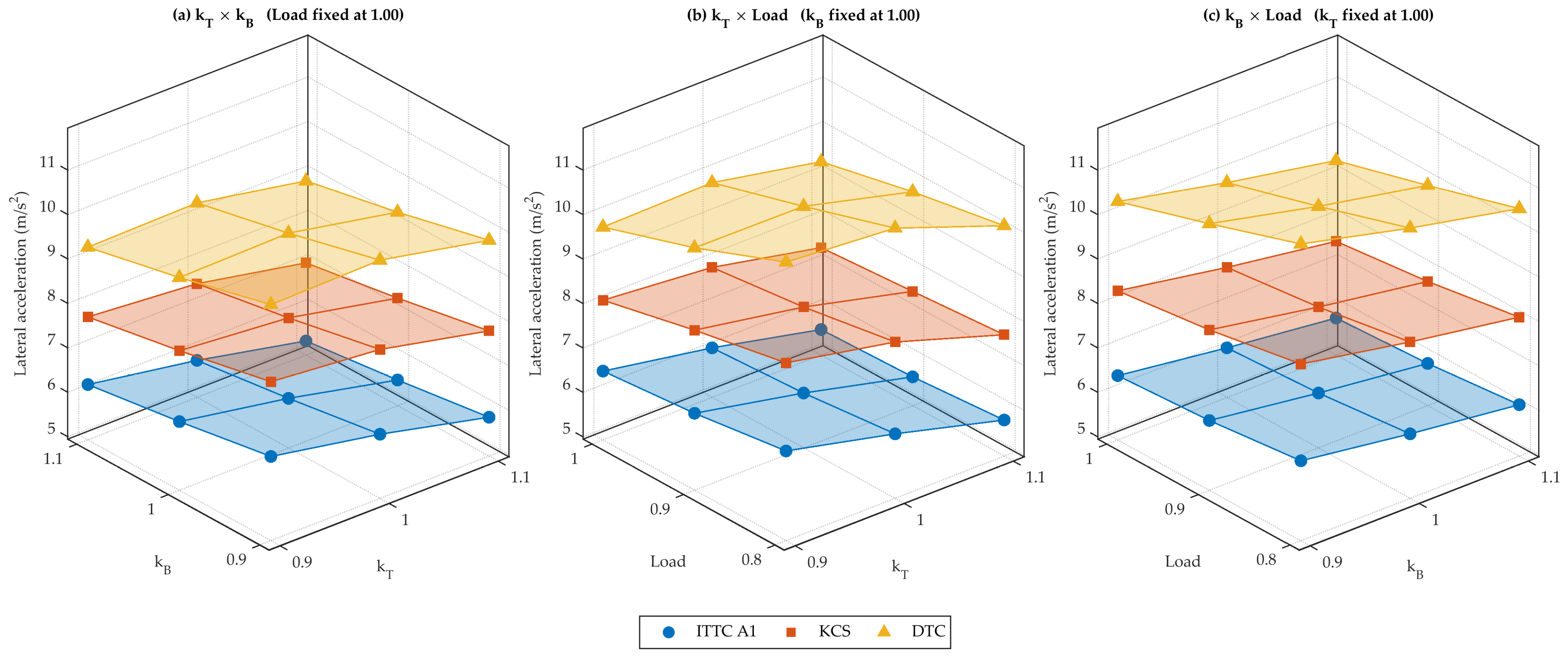
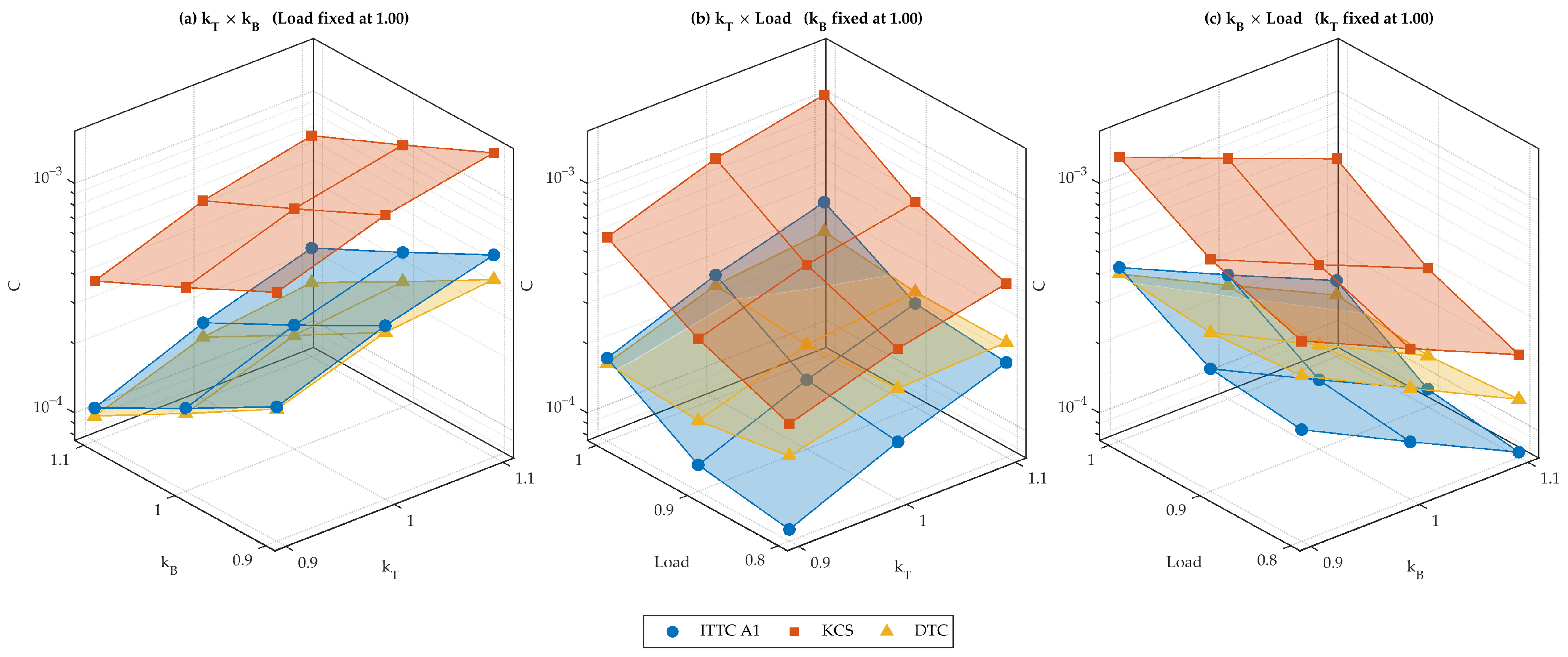

Disclaimer/Publisher’s Note: The statements, opinions and data contained in all publications are solely those of the individual author(s) and contributor(s) and not of MDPI and/or the editor(s). MDPI and/or the editor(s) disclaim responsibility for any injury to people or property resulting from any ideas, methods, instructions or products referred to in the content. |
© 2026 by the authors. Licensee MDPI, Basel, Switzerland. This article is an open access article distributed under the terms and conditions of the Creative Commons Attribution (CC BY) license.