A Comparative Fatigue Assessment of a Semi-Submersible FOWT Using Time- and Frequency-Domain Methodologies

Abstract

This study compares time-domain and frequency-domain fatigue assessment methodologies for the HiveWind semi-submersible floating offshore wind turbine (FOWT). Identical structural regions were selected from a global fatigue screening covering more than 16,000 hot spots. The time-domain approach combines Bladed–OrcaFlex coupled simulations with a high-fidelity Reduced Basis Finite Element Method (RB-FEM) structural model, whereas the frequency-domain approach combines linear wave-induced structural transfer functions with damage-equivalent turbine loads. The two approaches were compared at three representative structural details located at different positions within the floater. The results show a strong dependence of the agreement on structural location: the largest discrepancies occur at the central column–bracing connection, close to the wind-turbine load path, whereas substantially better agreement is obtained at a more distant column and in the heave-plate regions. The frequency-domain methodology requires substantially fewer computational resources, but its underlying linearization and DEL representation do not retain load sequence, relative phase, transient peaks, or nonlinear coupling effects. These results support a location-dependent assessment strategy in which detailed time-domain analyses are concentrated on fatigue-critical regions, while frequency-domain methods are used for preliminary assessment and less dynamically sensitive locations.

1. Introduction

Accurate fatigue life prediction is essential for the safe and cost-effective design of floating offshore wind platforms. Given the increasing complexity of these structures and the long design lives involved, it is crucial to evaluate the trade-offs between computational efficiency and predictive accuracy. Despite prior design and hydrodynamic investigations [1,2,3] emphasizing stability and mooring configurations, this study undertakes a comparative evaluation of time-domain and frequency-domain methodologies under realistic load spectra. The objective is to streamline fatigue assessment procedures without compromising the floater’s structural integrity over its 25-year service life.

Fatigue analysis in structural components has long been a foundational aspect of engineering design, particularly for systems subjected to cyclic or random loading. From early empirical approaches based on S-N curves [4,5] to advanced multiaxial and spectral models for marine materials [6], methodological evolution has significantly enhanced life prediction capabilities for complex systems. Traditionally, time-domain methods have been widely adopted due to their ability to capture transient and nonlinear behaviours in structural responses [7]. Techniques such as Rainflow counting; direct stress integration; and, more recently, deep learning models (e.g., LSTM and CNN networks) have been used to predict fatigue under multiaxial and non-stationary conditions [8]. In contrast, frequency-domain approaches have gained popularity in vibration fatigue due to their computational efficiency when dealing with stationary random loads [9,10]. The dynamic response of single-degree-of-freedom mechanical systems to stationary non-Gaussian random loads has also been investigated analytically by Sgamma et al. [11].

Recent research has increasingly explored combined time- and frequency-domain fatigue methodologies to balance computational efficiency and the representation of nonlinear structural response. Spectral approaches provide substantial computational advantages for stationary random processes [9,10,12], whereas time-domain methods retain synchronized histories for cycle identification and can represent transient effects and nonlinear coupling. For floating offshore wind turbines, these differences are particularly relevant because aerodynamic, hydrodynamic, mooring, and structural responses interact over multiple time scales. Abdelmoteleb and Bachynski-Polić [13] combined frequency-domain optimization with nonlinear coupled simulations for floating-wind mooring systems, while Shin et al. [14] investigated frequency-domain response-based approaches for FOWTs.

Reduced-order structural methods provide a further route to improving the efficiency of high-fidelity time-domain calculations. Knezevic et al. [15] demonstrated the application of RB-FEM to a structural-integrity assessment of a semi-submersible FOWT. The present study builds on these developments by directly comparing time-domain RB-FEM and conventional frequency-domain finite element fatigue assessments at identical structural regions of the same semi-submersible FOWT. The comparison focuses on both predicted fatigue damage and computational requirements, with particular attention to the influence of structural location and turbine-induced loading.

Throughout this manuscript, RB-FEM denotes the Reduced Basis Finite Element Method used for the time-domain structural solution.

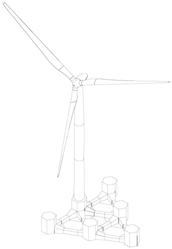
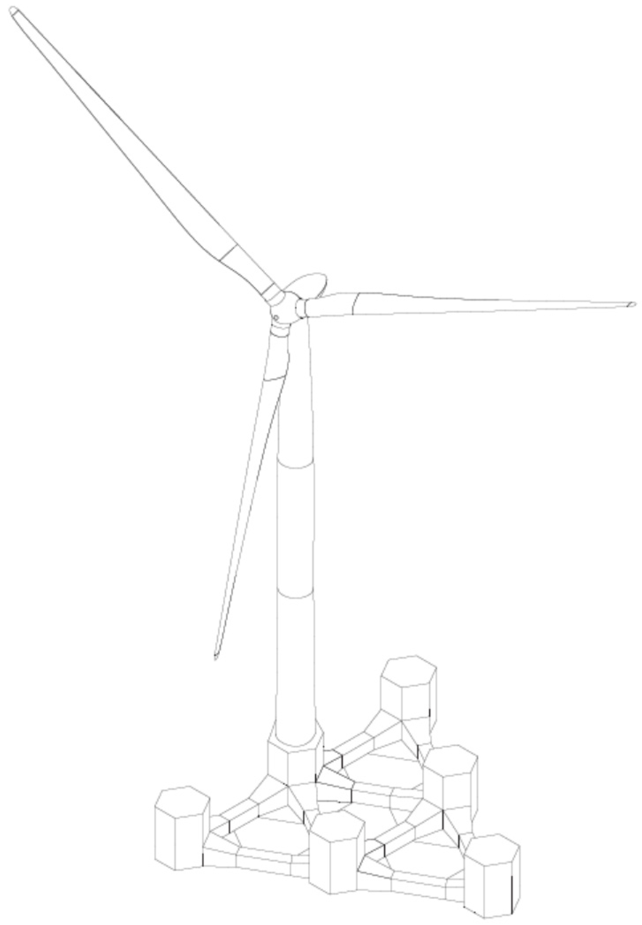
The case study considers a 25-year design life and a site off the Gulf of Roses in the northern Spanish Mediterranean, at water depths of approximately 120–140 m (42.126° N–42.158° N and 3.394° E–3.437° E). The HiveWind floater comprises six vertical columns interconnected by lower bracings and is based predominantly on flat-panel construction to facilitate modular fabrication and assembly (Figure 1) [16]. The floater’s main particulars are summarized in Table 1. The selected wind turbine (Table 2) is the MingYang MySE11-230 Offshore [17,18]. The objective is to compare fatigue-damage predictions and computational requirements of the two methodologies and to identify the practical implications of their modelling assumptions for offshore structural design.

Figure 1. The geometry of the HiveWind floater.

Table 1. HiveWind main particulars [authors’ design data].

Parameter	Value
Draft	8.00 m
Column length	17.00 m
External-column diameter	14.00 m
Central-column diameter	15.20 m
Pontoon length	27.87 m
Pontoon height	3.80 m
Pontoon width	3.60 m
Principal rotational inertias, (Ixx, Iyy, Izz)	(23.609, 23.559, 12.873) × 106 t·m2
Products of inertia (Ixy, Ixz, Iyz)	(−1.07 · 103, −3.93 · 106, 6.97 · 102) t·m2
Center of gravity (xG, yG, zG)	(21.4, 0, 17.4) m
Center of buoyancy (xB, yB, zB)	(21.4, 0, 4.0) m

Table 2. Public MySE11-230 Offshore main particulars [17].

Parameter	Value
Rated power	11,000 kW (11 MW)
Rotor diameter	230 m
Swept area	41,584 m2
Number of blades	3
Blade material	Carbon-glass hybrid
Hub height above water	126 m (adjustable)
Tower type	Conical steel tubular
Cut-in wind speed	3.0 m/s
Rated wind speed	11 m/s
Cut-out wind speed	25.0 m/s
Survival wind speed	78.8 m/s
Gearbox type	Hybrid
Generator type	PMSG (Permanent Magnet Synchronous Generator)
Grid connection	IGBT, 50/60 Hz
Tower mass	600 t

The global model origin, $O=\left(0\right|0\left|0\right)$, is located at the centreline of the central Column 1C at the platform keel (baseline). The positive x-axis points from Column 1C towards Column 3C, the positive y-axis points towards port, and the positive z-axis points upwards from the platform keel.

2. Materials and Methods

The HiveWind structural model was generated from the project CAD geometry and design scantlings. The model represents the main columns, bracings, pontoons, watertight compartments, ballast distribution, and structural details required for global and local fatigue assessment.

The station-keeping system comprises three catenary mooring lines of identical composition and nominal length. Each line consists of a 700 m long studless Grade R4 chain with a nominal diameter of 160 mm. The chain has a mass per unit length of 512 kg/m in air, a minimum breaking load of 21,885 kN, and an axial stiffness EA = 2.031 × 10⁶ kN. The line azimuths are 150°, 30°, and 270° NED for Lines 1–3, respectively. The corresponding horizontal anchor-to-fairlead distances are 656.1, 656.5, and 657.3 m, and the seabed elevations at the anchors are −138.7, −136.9, and −132.4 m. The fairleads are located at keel level. At the nominal platform position, the fairlead tensions are 1464, 1461, and 1453 kN, with corresponding line angles of 51.7°, 51.6°, and 51.4° from the horizontal. The horizontal tension component is approximately 907 kN for all three lines, and the corresponding anchor tensions are 475, 478, and 485 kN. The mooring configuration and line properties correspond to the verified OrcaFlex model used in the station-keeping analysis.

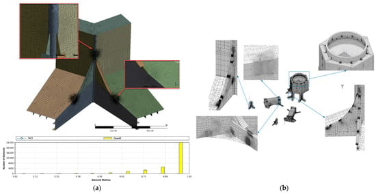
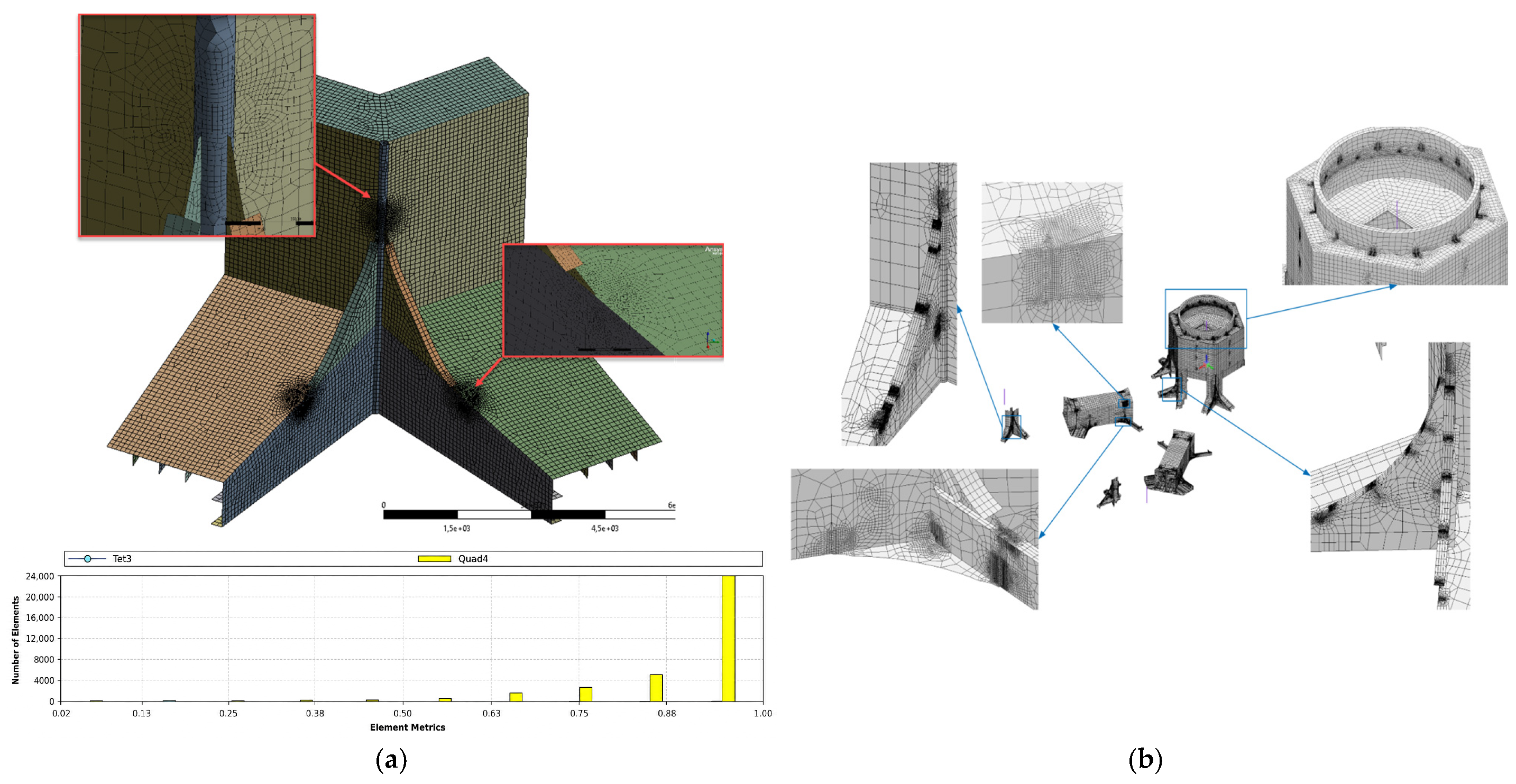
Prior to fatigue assessment, both structural models underwent mesh refinement and quality checks. The Ansys (2024R2 version) frequency-domain model was locally refined at structural joints and bracing connections to capture stress gradients, whereas the time-domain RB-FEM model (Akselos [19]) used targeted refinement in fatigue-critical components (Figure 2).

Figure 2. Representative local meshes used in the fatigue assessment: (a) Ansys frequency-domain refined submodel; (b) Akselos RB-FEM time-domain model.

For the frequency-domain analysis, the Ansys global finite element model comprised 139,168 predominantly quadrilateral shell elements and 116,086 nodes, with local fatigue shell submodels refined using a quad-dominant mesh. In fatigue-critical regions, a characteristic element size of approximately t × t was used, where t denotes the representative net thickness of the thinner adjoining plate. The element aspect ratio was close to unity, with a gradual transition towards the surrounding global mesh. For the time-domain analysis, the detailed RB-FEM model comprised 911,629 quadrilateral shell elements and 868,026 nodes, corresponding to approximately 5.2 million degrees of freedom; 11 of the 28 structural components were locally refined. Within detailed fatigue regions, the mesh was refined from approximately t × t to (t/3) × (t/3).

Mesh-quality checks were based on the Scaled Jacobian and element Shape metrics, both maintained above 0.2 in the fatigue-relevant regions. For both models, mesh convergence was assessed by successive local mesh refinements at the fatigue-critical hot-spot locations. Convergence was considered achieved when the variation in extrapolated hot-spot stress between two successive mesh refinements was below 5%. This 5% threshold is a study-specific numerical tolerance, not a universal requirement of DNV-RP-C203. Local refinement was limited to a minimum characteristic element size of approximately t/3. The convergence assessment used the same load case, stress-extraction path, and DNV-RP-C203 Method A extrapolation procedure for each refinement level.

The same study-specific 5% tolerance is used for the temporal-resolution check, where it applies to accumulated fatigue damage rather than hot-spot stress.

Aerodynamic and operational loading from the wind turbine was generated using Bladed simulations. These simulations provided either time-series data for each Design Load Case (DLC) used in the time-domain study or Damage Equivalent Loads (DELs) for the frequency-domain approach. All simulations were location-specific and synchronized with environmental parameters, including wind speed, wave height, and directionality based on the site data.

For the frequency-domain pathway, each Damage Equivalent load (DEL) represents the constant-amplitude load range that produces the same Miner damage as the variable-amplitude aeroelastic history for a specified S-N slope m and reference number of cycles N_ref.

The turbine DEL input used for the frequency-domain assessment was supplied for MySE11-230. The selected inverse S–N slope was m = 4 and the reference cycle count was N_ref = 10⁷ for the 25-year assessment. These parameters define the turbine-load equivalence and are distinct from the S–N curves used to assess the local structural details. The DELs are expressed as load ranges. The supplier’s component-wise Markov cycle matrices are consistent with this reference-cycle normalization but do not retain synchronized histories between load channels. The underlying WTG load values are confidential (see Data Availability Statement).

$$DEL={\left[{\displaystyle \frac{{\sum }_{\mathrm{i}}{\mathrm{n}}_{\mathrm{i}}{\left(\mathsf{\Delta }{\mathrm{L}}_{\mathrm{i}}\right)}^{\mathrm{m}}}{{\mathrm{N}}_{\mathrm{r}\mathrm{e}\mathrm{f}}}}\right]}^{{\displaystyle \frac{1}{\mathrm{m}}}}$$

(1)

DEL equivalence is conditional on the selected S–N slope, reference cycle count, mean-load treatment and load-channel convention. For a fixed history, increasing m gives greater weight to the larger load ranges. A DEL does not retain the original history or the relative phases between load channels, and a local structural S–N category does not by itself identify the slope used in turbine DEL post-processing.

The fatigue assessment procedure follows DNV-RP-C203 [20]. Site conditions were described by a joint distribution of wave height, period and direction. For the wave contribution reported, this distribution was converted into representative regular-wave blocks, this distribution was converted into representative regular-wave blocks (RWB) and occurrence-derived cycle counts over 25 years. This is a deterministic block calculation rather than a reconstruction of fatigue cycles from a JONSWAP stress spectrum. First-order hydrodynamic pressures were obtained in Ansys AQWA and transferred to the structural model. The turbine contribution used the MySE DEL convention stated above. The time-domain assessment used the retained fatigue DLCs [21], with its own simulation histories and occurrence weights.

2.1. Screening Process

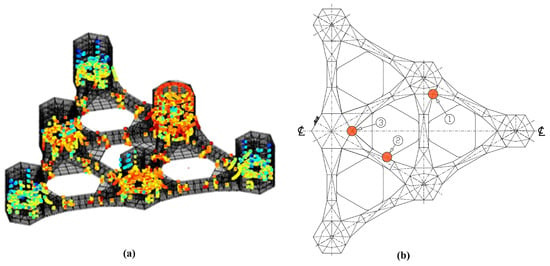
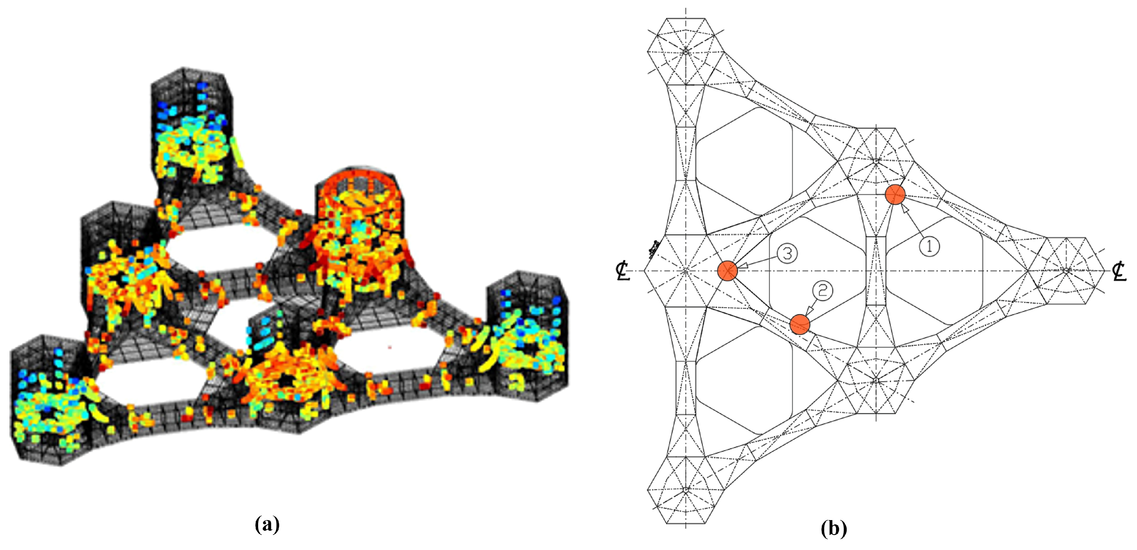
Response Amplitude Operators (RAOs) were used in the frequency-domain screening to compute stress responses across more than 16,000 critical hot-spot locations (Figure 3a). Effective stress was extracted using the Method A structural hot-spot stress procedure defined in DNV-RP-C203 [20], and fatigue damage was calculated with the Palmgren–Miner rule. Curve D in seawater with cathodic protection was used for submerged zones and curve D in air for topside elements. A Design Fatigue Factor (DFF) of 1.0 was adopted for this preliminary screening, and 25-year accumulated damage was calculated at each hot spot. For the subsequent detailed frequency-domain assessment, the S–N curve was assigned according to the applicable fatigue-detail category for each structural zone.The screening identified the structural regions subsequently assessed with both the frequency-domain and time-domain approaches. In the linear frequency-domain formulation, wave-induced stress is represented by first-order transfer functions; higher-order hydrodynamic contributions and material load-interaction effects are outside the scope of the method.

Figure 3. (a) More than 16,000 hot-spot locations from the global screening (blue dots candidates less damage—red dots candidates more damage); (b) structural details selected for the comparative assessment.

A separate preliminary time-domain screening dataset comprised 670 simulations, each 10 min in duration and sampled at 1 Hz. Together, these simulations represented a cumulative occurrence probability of 94.13%. These records were used only for fatigue-sensitive-region identification and ranking and were not used as the final quantitative time-domain dataset. For each hot spot, the fatigue damage obtained from simulation i was annualized according to Equation (2).

$${\mathrm{D}}_{annual}=\sum \left[p_i\ast \left({\displaystyle \frac{T_{year}}{{\mathrm{T}}_i}}\right)\ast {\mathrm{D}}_i\right]$$

(2)

where D_i is the fatigue damage accumulated during simulation i, T_i is the corresponding simulation duration, p_i is its normalized occurrence probability, and T_year denotes one year. The resulting annualized damage values were used solely for hot-spot screening and ranking.

For the detailed comparison, D25 denotes accumulated Miner damage over 25 years without multiplication by the Design Fatigue Factor. The two methods use this same basis. For a stationary long-term annualization, D25 = 25 D_annual. The conventional Miner exhaustion criterion is D25 = 1; the adopted design requirement is D25 ≤ 1/DFF, giving D25 ≤ 0.40 for DFF = 2.5. The value 0.40 is therefore an acceptance limit, not an upper bound on calculated damage. Screening with DFF = 1.0 is a separate stage.

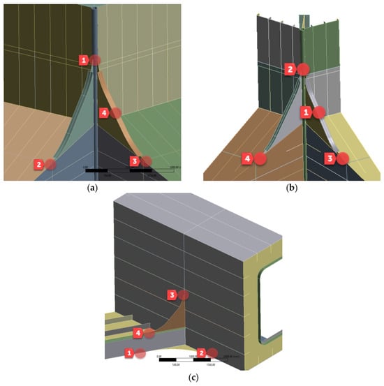
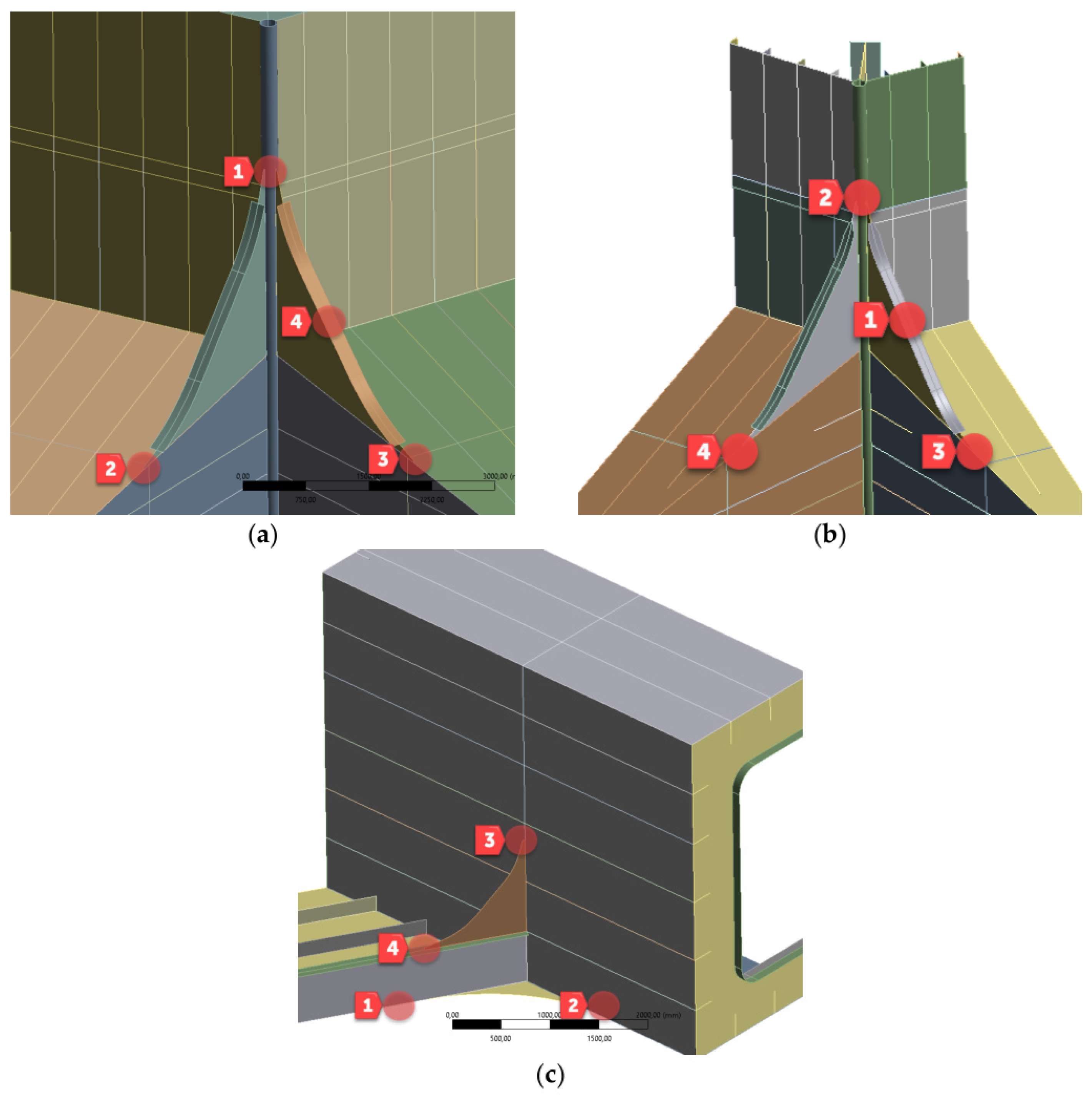
Based on the screening results, three structural locations were selected for the detailed time–frequency comparative assessment (Figure 3b): (1) the connection between column 2P and its bracings (C2P); (2) the heave plates (HP); and (3) the junction of column 1C with the central bracings (C1C). Figure 3b provides the platform-level location map, while Figure 4 gives enlarged views of the C1C, C2P, and HP structural components and their fatigue zones.

Figure 4. The fatigue assessment regions used for the comparison: (a) central column–bracing connection C1C; (b) column 2P–bracing connection C2P; (c) heave-plate region HP.

The selection was purposive: C1C represents the fatigue-sensitive connection on the turbine load-transfer path, C2P a more remote column–bracing connection, and HP the heave-plate region. These three regions sample different loading and geometric contexts; the global screening does not make the detailed comparison statistically representative of all hot spots or of other FOWTs.

In the preliminary frequency-domain assessment, highly loaded regions from global ULS cases were used to identify candidates for local fatigue assessment. This initial selection is distinct from the subsequent fatigue screening and does not establish a universal fatigue-criticality threshold.

2.2. Frequency-Domain Simulation Procedure

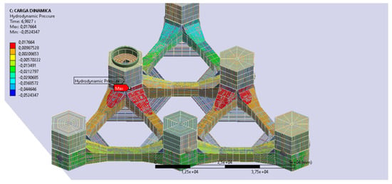
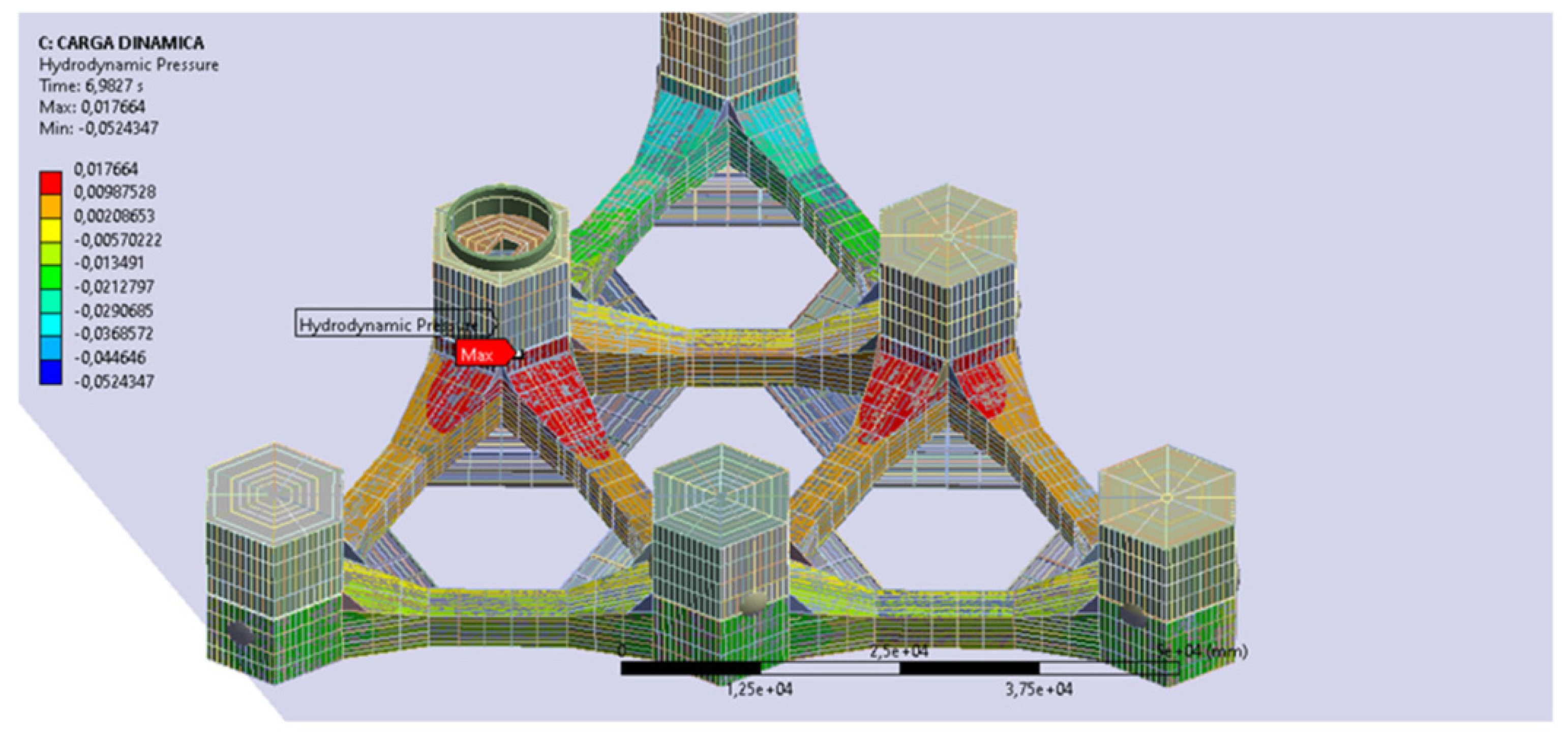
The frequency-domain analysis was performed using a global hydrodynamic–structural model. For each environmental state, first-order potential-flow calculations were performed in Ansys AQWA. The resulting wave-excitation, diffraction, and radiation pressures were integrated over the wetted surface and transferred to the Ansys Mechanical structural model. Figure 5 shows the hydrodynamic pressure and hydrostatic-variation loads implemented inthe global model. The structural model employed SHELL181 elements, a four-node Mindlin–Reissner shell formulation with six degrees of freedom per node, suitable for thin to moderately thick plated structures [22].

Figure 5. Hydrodynamic pressure (Pa) and hydrostatic-variation loads implemented in the global model.

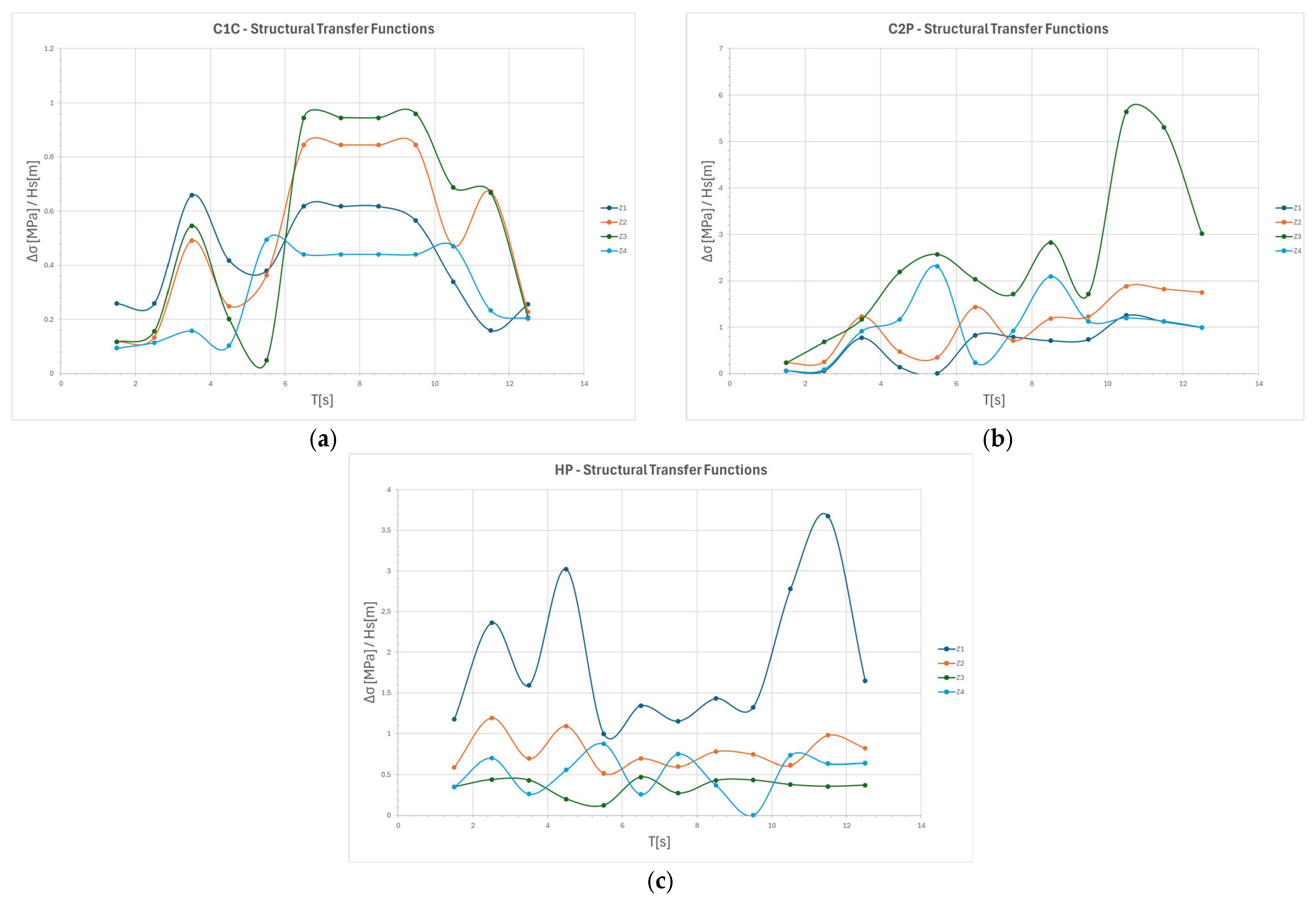
Upon completion of the hydrodynamic calculations, a submodel was used for each selected detail. Structural hot-spot stress ranges were extracted from the representative regular-wave blocks using the Method A procedure described in Appendix A.4. The response at each block height, period and direction was paired with the corresponding 25-year cycle count. Wave damage was calculated as the sum of n_i/N_i over those blocks, using the structural S–N category assigned to the zone. The plotted transfer functions in Figure A2 describe the linear response used to obtain the block stresses; they do not imply that Rayleigh or Dirlik spectral cycle counting was applied.

The three locations identified in Figure 3b are shown in detail in Figure 4. Each detail is divided into fatigue assessment zones; for example, C1C (Z1) denotes Zone 1 of the connection between central Column 1C and its bracing, as shown in Figure 4a.

2.3. Time-Domain Simulation Procedure

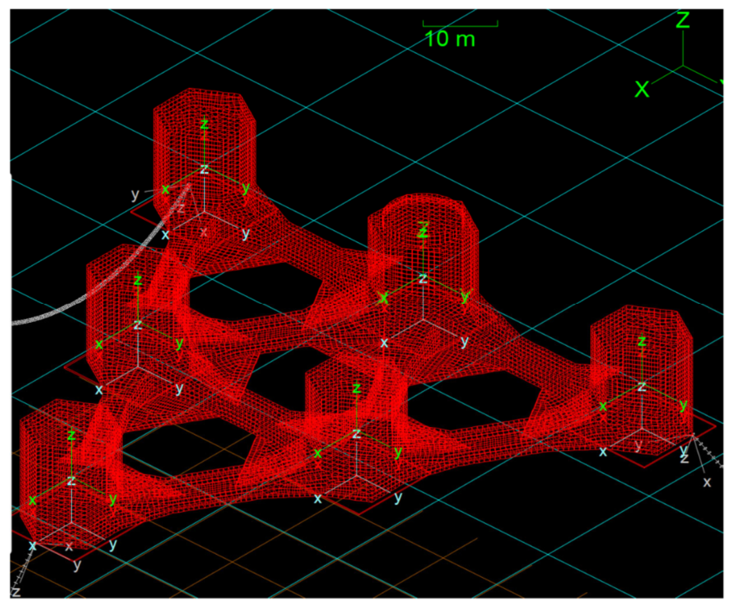
The time-domain fatigue analysis was performed using the RB-FEM structural model driven by synchronized outputs from the coupled Bladed–OrcaFlex simulations. Bladed provided the aeroelastic wind-turbine loads, whereas OrcaFlex provided platform motions, hydrodynamic response, and mooring-line loads. These quantities were mapped onto the structural model to obtain time histories of stress at the fatigue-critical locations. Rainflow cycle counting and the Palmgren–Miner rule [5,20] were then applied to calculate cumulative fatigue damage. The coupled OrcaFlex model is shown in Figure 6.

Figure 6. The coupled OrcaFlex model used for the time-domain simulations.

Rainflow uses the stress history to identify stress ranges and cycle counts. The subsequent linear Palmgren–Miner accumulation is insensitive to the order of the already counted cycles and does not model material sequence or overload-interaction effects. Retaining a time history should therefore not be interpreted, as including these material effects in the damage law.

Fully coupled time-domain simulations were performed using the coupled Bladed–OrcaFlex workflow for the critical Design Load Cases (DLCs). The original detailed fatigue dataset comprised 1339 one-hour simulations sampled at 5 Hz. To assess the adequacy of the temporal discretization for fatigue analysis, the simulations were subsequently evaluated at higher sampling rates up to 20 Hz (Δt = 0.05 s). This corresponds to approximately 33 samples per cycle at the upper frequency of interest of 0.6 Hz. Temporal-resolution convergence was assessed by comparing the Rainflow-based annual fatigue damage obtained at 5, 10, and 20 Hz at representative fatigue-critical hot spots. Using the 20 Hz solution as the reference, convergence was considered achieved when the change in accumulated fatigue damage between successive temporal resolutions was below 5%. The maximum difference between the 10 and 20 Hz solutions was 4.89%, confirming that the selected temporal resolution provides a converged fatigue estimate. Each simulation provided time histories of the platform six-degree-of-freedom motions, mooring-line tensions, tower-base forces and moments, and hydrodynamic loading parameters. The first 300 s of each one-hour record were discarded to remove initialization and load-ramp transients. Stationarity of the remaining response was verified by checking the temporal stability of the mean and standard deviation of representative motions, loads, and hot-spot stresses. The consistency of the Rainflow cycle rate and fatigue-damage rate between consecutive windows was also checked. Only the stationary portion of the retained high-resolution records was used for the final Rainflow cycle counting and fatigue-damage assessment. Site-specific occurrence probabilities were then applied to obtain the corresponding annual fatigue damage.

2.3.1. Load Mapping Methodology

Permanent (G) and environmental (E) load components were decomposed and mapped onto the approximately 5.2-million-degree-of-freedom RB-FEM model [15]. The principal load categories are listed in Table 3.

Table 3. Load categories.

Load Category	Permanent (G)	Environmental (E)
Gravity	Static self-weight on shell subdomains	Time-varying gravity vector induced by platform motions
Hydrostatic	Buoyancy pressure at the mean water level	Linearized hydrostatic stiffness for heave, pitch, and roll
Ballast	Hydrostatic pressure due to water in ballast tanks	Equivalent point masses (RBE3) representing dynamic ballast inertia
Moorings	Pre-tension in mooring lines	Time-series of dynamic mooring tensions
Tower Base	Static tower-mounted loads	Time histories of dynamic tower-base forces and moments
Morison Drag	–	Recomputed drag on the beam skeleton imported from OrcaFlex
Diffraction & Radiation	–	Time-domain pressures interpolated from the hydrodynamic database
Inertia	–	Mass-weighted acceleration loads

Environmental loads were reconstructed by combining Bladed aeroelastic outputs with OrcaFlex/AQWA hydrodynamic outputs: Morison drag was recomputed using the same beam geometry and drag coefficients as in OrcaFlex. Diffraction and radiation pressures were interpolated onto the structural mesh, and ballast inertia was applied via discrete point-mass connectors. Bladed does not generate Morison, diffraction, or radiation loads in this workflow. Morison drag is recomputed from the relative fluid velocity and member geometry using the Morison drag force per unit length, F_D, as defined in Equation (3).

$${\mathrm{F}}_d=0.5\ast \mathsf{\rho }\ast \mathrm{C}\mathrm{d}\ast \mathrm{D}\ast \left|\mathrm{u}\mathrm{r}\right|\ast \mathrm{u}\mathrm{r}$$

(3)

The Morison drag coefficients used in the time-domain model were transferred directly from the verified OrcaFlex model together with the corresponding beam-skeleton geometry and drag diameter. The adopted coefficients and numerical drag diameters are summarized in Table 4. The apparently large numerical C_d values result from the equivalent slender-beam representation and must therefore be interpreted together with the corresponding numerical drag diameter. The reconstructed Morison loads were subsequently checked against the corresponding OrcaFlex loads, showing close agreement between the two implementations.

Table 4. Morison drag parameters transferred from OrcaFlex.

Cd,y	Cd,x	Normal Drag Diameter, D [m]	Morison Element
51,000	51,000	1.40 × 10−4	Columns SL
255,000	255,000	1.40 × 10−4	Columns SM
500,000	500,000	1.40 × 10−4	Columns SU
554,000	554,000	1.40 × 10−4	Column 1C SL
277,000	277,000	1.40 × 10−4	Column 1C SM
543,000	543,000	1.40 × 10−4	Column 1C SU

Cd,z = 0 for all Morison element types. SL, SM and SU denote the lower, middle and upper Morison segments, respectively; columns refers to the external columns, whereas Column 1C denotes the turbine-supporting column 1C.

2.3.2. Verification of Load Mapping

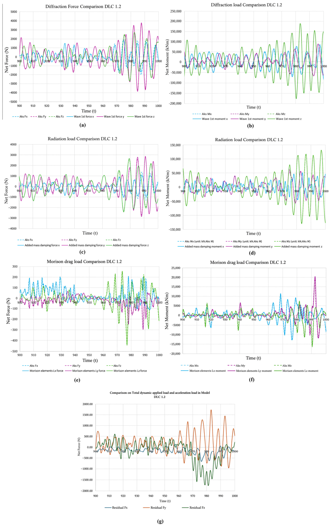
Load mapping was assessed by comparing the reconstructed diffraction, radiation, Morison-drag, and hydrostatic force and moment histories with the corresponding coupled-analysis results over representative 100 s intervals. Force and moment residuals were calculated using a consistent sign convention and reference point and were retained as measures of mapping uncertainty rather than assumed to vanish. Subsequent Rainflow cycle counting and Palmgren–Miner accumulation were performed in accordance with DNV-RP-C203 [20] after stress analysis in the RB-FEM model. The force and moment residuals are denoted RF(t) and RM(t), and the corresponding relative residuals are denoted ηF and ηM.

$${\mathit{R}}_F\left(t\right)={\mathit{F}}_{inertia}\left(t\right)+{\displaystyle \sum _{j=1}^{N_F}}{\mathit{F}}_{j,applied}\left(t\right),$$

(4)

$${\mathit{R}}_M\left(t\right)={\mathit{M}}_{inertia}\left(t\right)+{\displaystyle \sum _{j=1}^{N_M}}{\mathit{M}}_{j,applied}\left(t\right),$$

(5)

$${\eta }_F={\displaystyle \frac{\underset{t}{max}∥{\mathit{R}}_F\left(t\right)∥}{\underset{t}{max}∥{\displaystyle {\sum }_{j=1}^{N_F}}{\mathit{F}}_{j,applied}\left(t\right)∥}},$$

(6)

$${\eta }_M={\displaystyle \frac{\underset{t}{max}∥{\mathit{R}}_M\left(t\right)∥}{\underset{t}{max}∥{\displaystyle {\sum }_{j=1}^{N_M}}{\mathit{M}}_{j,applied}\left(t\right)∥}}.$$

(7)

The load-mapping verification shows non-zero residual excursions shows non-zero residual excursions; these are retained as numerical uncertainty associated with load mapping and omitted global components rather than interpreted as evidence of exact equilibrium.

A global force or moment residual is a load-transfer diagnostic, not a direct measure of local fatigue-damage error. Its influence depends on the spatial distribution of the mapping discrepancy and on the stress response at the hot spot. No quantitative propagation of the mapping residual into local damage is established by the plotted load comparisons.

3. Results

3.1. Screening

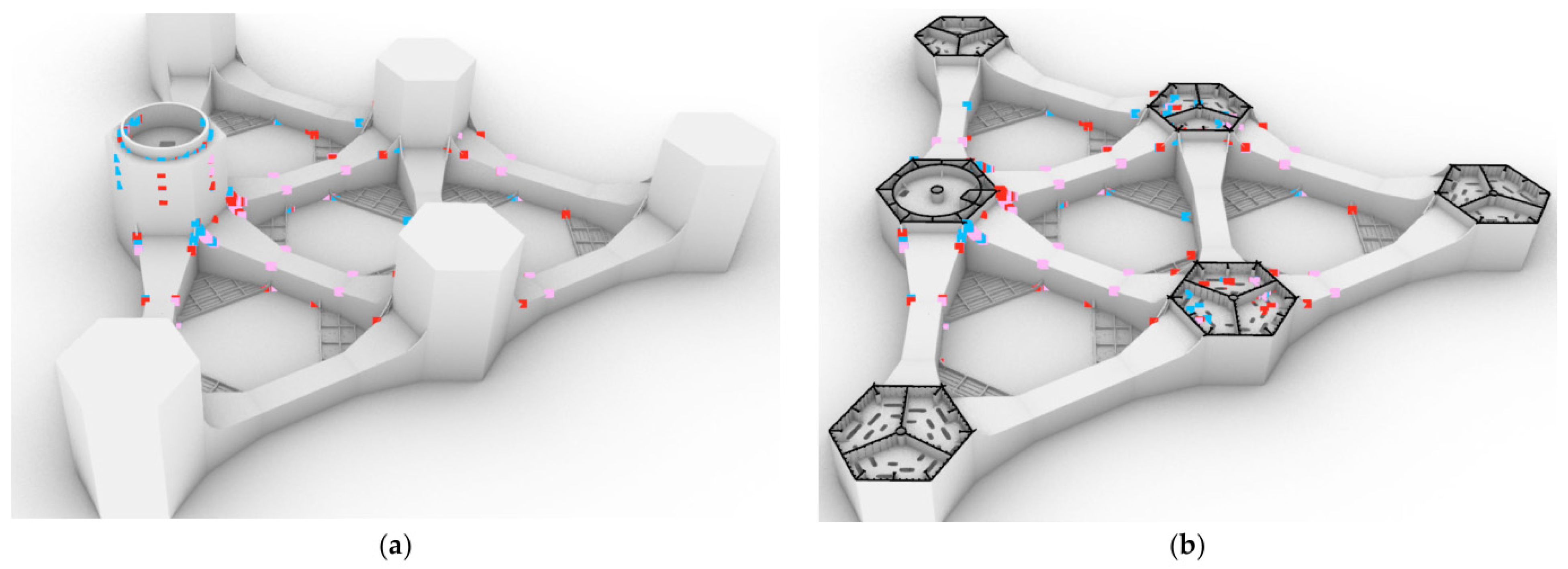
Figure 7 summarizes the screening results. The most fatigue-sensitive regions are concentrated around the transition piece and the connections between the bracings and central Column 1C, close to the wind-turbine load-transfer path. Regions farther from this load-transfer path, including the heave-plate–bracing interfaces and the connections of Columns 2P and 2S to their bracings, generally exhibit lower screening damage. For clarity, Figure 7 and Figure 8 show representative hot spots retained from the screening, including those associated with structural openings.

Figure 7. (a) The global fatigue-screening view; (b) the representative screening section of the structure. Red, Pink and blue indicate high, medium, and low damage, respectively.

Figure 8. The time-domain screening fatigue-damage map: (a) hot spots with damage below 0.04; (b) hot spots with damage from 0.04 to 0.10. Point colours follow the damage scale displayed in each panel.

3.2. Frequency-Domain Results

The frequency-domain analysis used four CPU cores and had a reported campaign duration of approximately 144 h. Table 5 reports the regular-wave block and turbine-DEL contributions to the 25-year damage without DFF multiplication. Their sum is the combined estimate used in this workflow; it is not a separately validated simultaneous-load fatigue result. All tabulated damage values are displayed with six decimal places; calculations retain the unrounded inputs.

Table 5. Frequency-domain damage accumulated over 25 years without DFF multiplication. The wave contribution uses occurrence-based regular-wave blocks. All damage values are displayed with six decimal places. Totals are calculated before rounding and may differ by one unit in the last decimal place from the sum of the components displayed. The design acceptance limit is 0.40 for DFF = 2.5.

Detail	Zone	S-N Curve	Wave Damage	DEL Damage	Total Damage
C1C	Z1	E	0.003076	0.229648	0.232724
	Z2	E	0.173456	0.000660	0.174116
	Z3	E	0.226430	0.075726	0.302155
	Z4	E	0.000045	0.000045	0.000091
C2P	Z1	C	0.000046	0.000015	0.000061
	Z2	E	0.000909	0.000412	0.001321
	Z3	E	0.012712	0.057704	0.070416
	Z4	C	0.000705	0.000020	0.000725
HP	Z1	C	0.000251	0.213650	0.213902
	Z2	C	0.000034	0.000588	0.000622
	Z3	E	0.000655	0.000001	0.000656
	Z4	E	0.000672	0.002956	0.003628

3.3. Time-Domain Results

The complete time-domain workflow was executed on a high-performance computing system using up to 150 CPU cores. The reported campaign duration was approximately 720 h. Load-transfer fidelity was evaluated by comparing synchronized time-series loads from the coupled Bladed–OrcaFlex analysis with the net forces and moments reconstructed in the structural model. Bladed provided aeroelastic tower loads, while OrcaFlex supplied platform motions, hydrodynamic actions, and mooring tensions. Morison drag was independently recomputed from the OrcaFlex kinematics for comparison. Over the representative 100 s DLC 1.2 interval shown in Figure 9, the non-zero force and moment residual histories were assessed using the definitions in Section 2.3.2 and retained as mapping uncertainty.

Figure 9. (a) Diffraction-force comparison; (b) diffraction-moment comparison; (c) radiation-force comparison; (d) radiation-moment comparison; (e) Morison-drag force comparison; (f) Morison-drag moment comparison; (g) total force residual.

Figure 9. (a) Diffraction-force comparison; (b) diffraction-moment comparison; (c) radiation-force comparison; (d) radiation-moment comparison; (e) Morison-drag force comparison; (f) Morison-drag moment comparison; (g) total force residual.

The detailed fatigue assessment comprised 1175 simulations under DLC 1.2 and 164 simulations under DLC 6.4. Each simulation was weighted by its site-specific occurrence probability. The retained simulation set represented 97.7% of the total occurrence probability, and the retained probabilities were subsequently normalized to unity for the final damage calculation.

The 97.7% occurrence coverage refers to the detailed retained dataset, whereas 94.13% refers to the separate preliminary screening dataset. Renormalization conditions the detailed damage estimate on the retained states; probability coverage alone does not establish that the fatigue contribution of omitted states or other DLCs is negligible. The conclusions are restricted to the retained loading set. The retained DLCs define the available detailed comparison, not a complete design-load assessment. The remaining 2.3% of occurrence probability is excluded from this estimate; renormalization does not recover its damage contribution. Other DLCs would require their own load histories and fatigue weighting before extending the conclusions to the full design-load envelope.

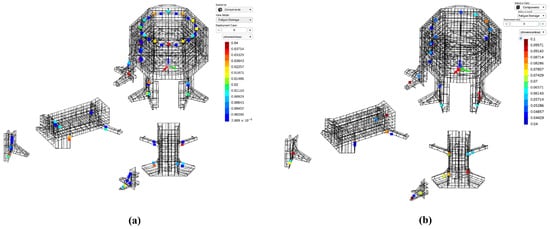
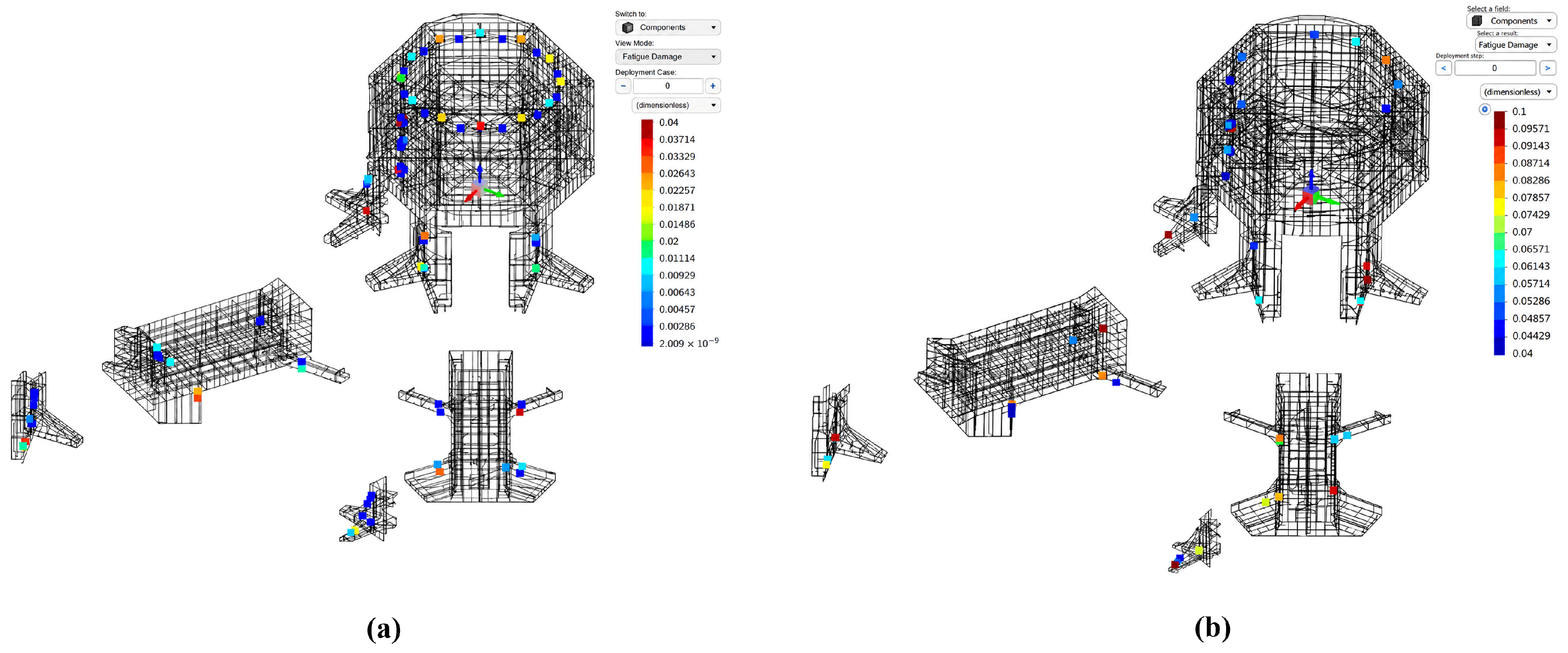
Figure 10 shows the time-domain damage distributions for the central-column bracing details in panel (a) and the external-column bracing details in panel (b). The panels are identified by structural location. The solver screenshots are labelled as one-year fatigue output and should be distinguished from the unfactored 25-year damage used for the method comparison in Figure 11.

Figure 10. Time-domain fatigue-damage maps: (a) central-column bracing details; (b) external-column bracing details. Point colours follow the scale shown in each solver screenshot, labelled as one-year fatigue output. These maps do not display DFF-based acceptance limits.

Figure 10. Time-domain fatigue-damage maps: (a) central-column bracing details; (b) external-column bracing details. Point colours follow the scale shown in each solver screenshot, labelled as one-year fatigue output. These maps do not display DFF-based acceptance limits.

Figure 11. The paired unfactored 25-year damage for (a) C1C, (b) C2P and (c) HP. Every point is identified by its Table 6 zone. Both axes are logarithmic and use the same limits within each panel; dashed lines indicate equal damage (TD = FD). The r values are Pearson coefficients calculated from the original, untransformed damage pairs (n = 4 per panel). The DFF = 2.5 acceptance limit is 0.40 and does not rescale the damage values. The TD results use the retained DLC 1.2 and DLC 6.4 set; the FD results combine site-occurrence RWB and turbine DELs rather than a separately matched DLC group.

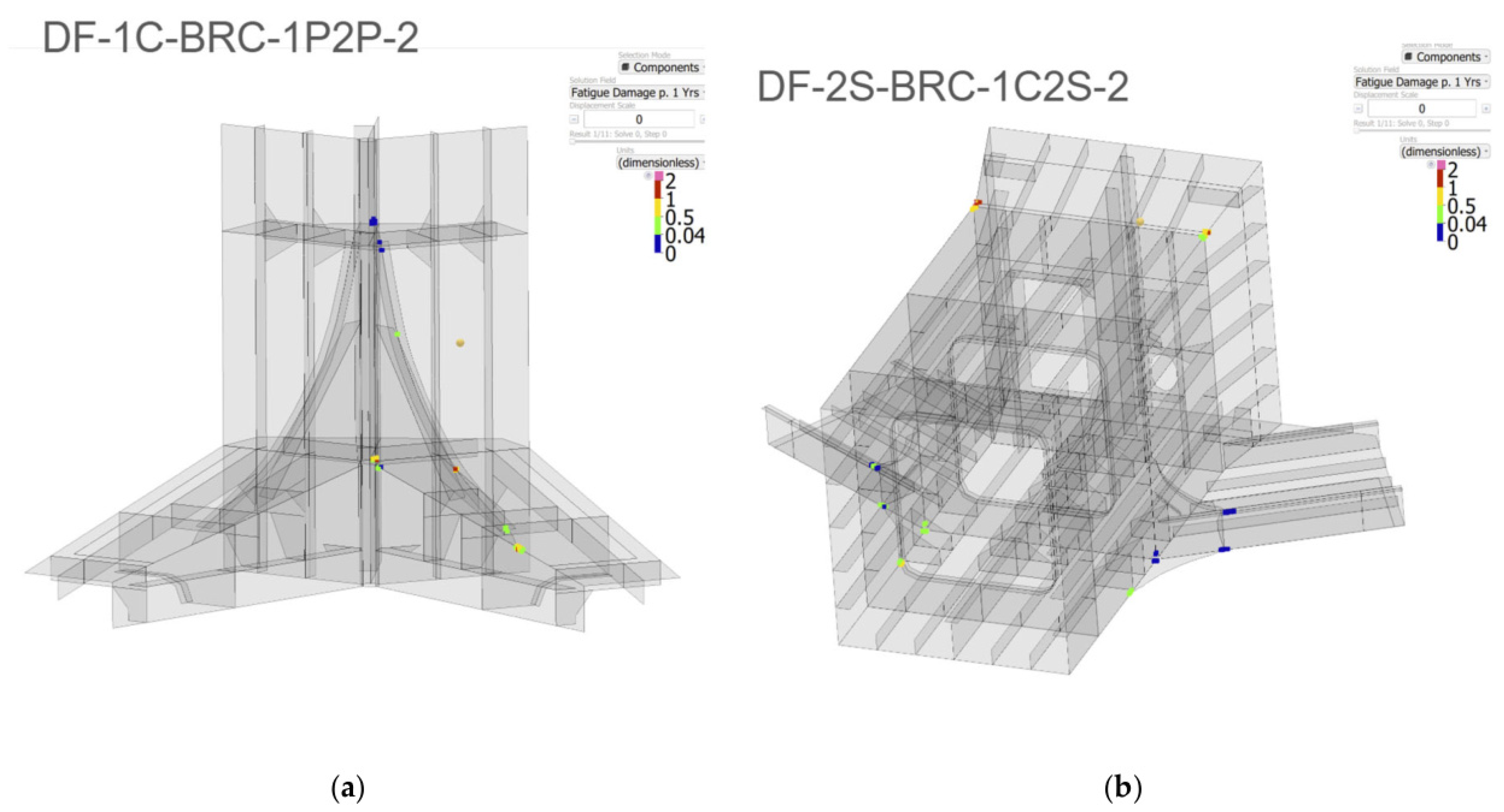
Figure 11. The paired unfactored 25-year damage for (a) C1C, (b) C2P and (c) HP. Every point is identified by its Table 6 zone. Both axes are logarithmic and use the same limits within each panel; dashed lines indicate equal damage (TD = FD). The r values are Pearson coefficients calculated from the original, untransformed damage pairs (n = 4 per panel). The DFF = 2.5 acceptance limit is 0.40 and does not rescale the damage values. The TD results use the retained DLC 1.2 and DLC 6.4 set; the FD results combine site-occurrence RWB and turbine DELs rather than a separately matched DLC group.

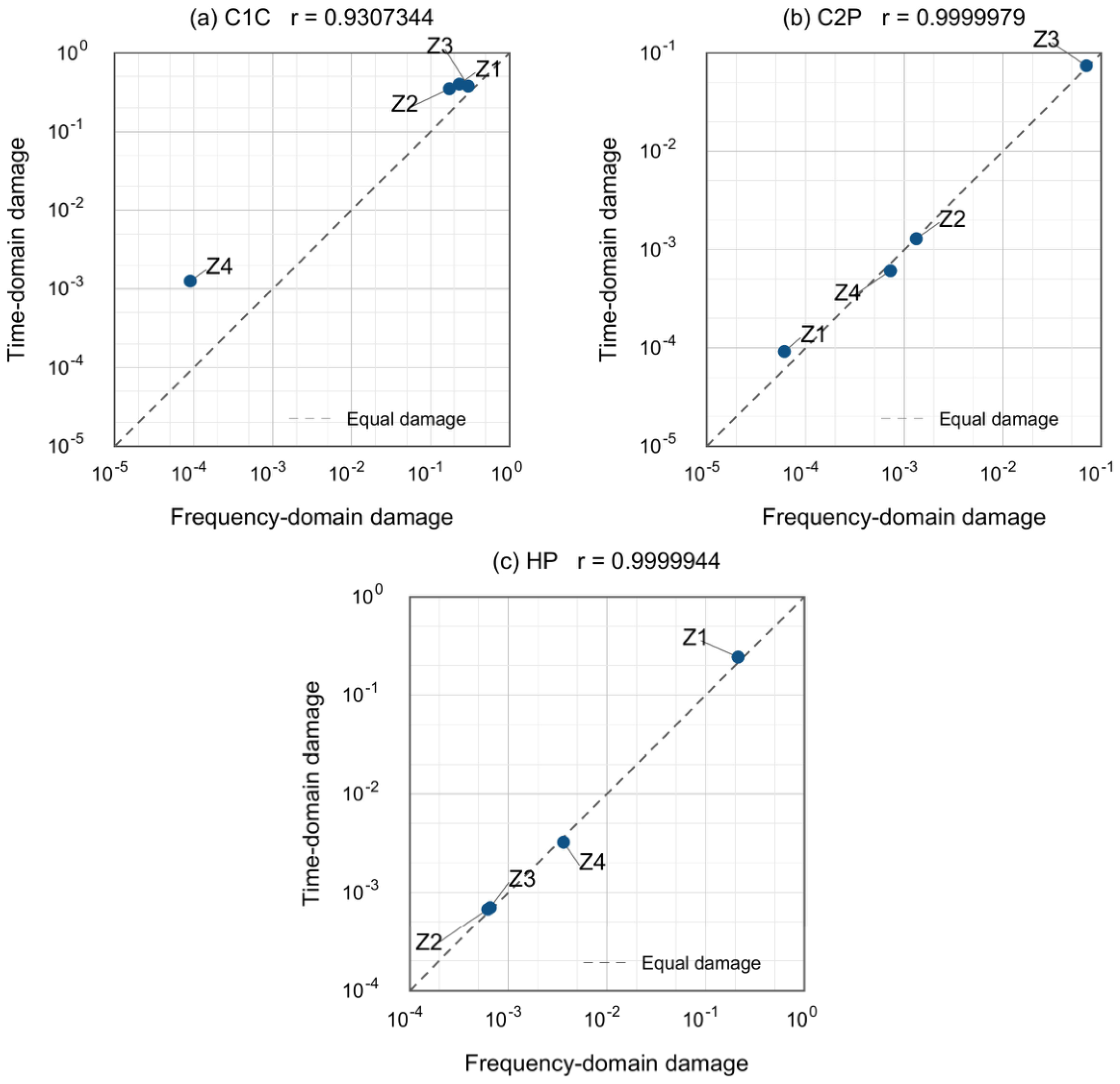
Table 6. The paired 25-year fatigue damage for all twelve zones without DFF multiplication. FD denotes the total in Table 5 and TD the time-domain result. Damage values have six decimal places. Ratios and signed differences use the unrounded inputs, with TD as the denominator. They therefore cannot always be reproduced exactly from the rounded values displayed here. The larger FD contribution is identified from the separate wave and turbine estimates in Table 5. This label describes the FD damage split, not the dominant physical cause of the FD–TD discrepancy. Similar contributions are labelled comparable.

Detail	Zone	Larger FD Contribution	FD Damage	TD Damage	FD/TD	Difference (%)
C1C	Z1	Turbine	0.232724	0.398952	0.583337	−41.67
C1C	Z2	Wave	0.174116	0.348965	0.498950	−50.10
C1C	Z3	Wave	0.302155	0.375896	0.803826	−19.62
C1C	Z4	Comparable	0.000091	0.001257	0.072135	−92.79
C2P	Z1	Wave	0.000061	0.000092	0.659975	−34.00
C2P	Z2	Wave	0.001321	0.001292	1.022100	+2.21
C2P	Z3	Turbine	0.070416	0.074023	0.951280	−4.87
C2P	Z4	Wave	0.000725	0.000609	1.189992	+19.00
HP	Z1	Turbine	0.213902	0.243204	0.879516	−12.05
HP	Z2	Turbine	0.000622	0.000676	0.919334	−8.07
HP	Z3	Wave	0.000656	0.000701	0.936102	−6.39
HP	Z4	Turbine	0.003628	0.003231	1.122924	+12.29

Table 6. The paired 25-year fatigue damage for all twelve zones without DFF multiplication. FD denotes the total in Table 5 and TD the time-domain result. Damage values have six decimal places. Ratios and signed differences use the unrounded inputs, with TD as the denominator. They therefore cannot always be reproduced exactly from the rounded values displayed here. The larger FD contribution is identified from the separate wave and turbine estimates in Table 5. This label describes the FD damage split, not the dominant physical cause of the FD–TD discrepancy. Similar contributions are labelled comparable.

Detail	Zone	Larger FD Contribution	FD Damage	TD Damage	FD/TD	Difference (%)
C1C	Z1	Turbine	0.232724	0.398952	0.583337	−41.67
C1C	Z2	Wave	0.174116	0.348965	0.498950	−50.10
C1C	Z3	Wave	0.302155	0.375896	0.803826	−19.62
C1C	Z4	Comparable	0.000091	0.001257	0.072135	−92.79
C2P	Z1	Wave	0.000061	0.000092	0.659975	−34.00
C2P	Z2	Wave	0.001321	0.001292	1.022100	+2.21
C2P	Z3	Turbine	0.070416	0.074023	0.951280	−4.87
C2P	Z4	Wave	0.000725	0.000609	1.189992	+19.00
HP	Z1	Turbine	0.213902	0.243204	0.879516	−12.05
HP	Z2	Turbine	0.000622	0.000676	0.919334	−8.07
HP	Z3	Wave	0.000656	0.000701	0.936102	−6.39
HP	Z4	Turbine	0.003628	0.003231	1.122924	+12.29

The largest time-domain damage among the twelve paired zones is D25 = 0.398952 at C1C Z1, compared with FD = 0.232724. All twelve FD estimates and all twelve TD estimates are below the adopted acceptance limit of 0.400000 for DFF = 2.5. The maximum TD value is close to that limit, and agreement between the workflows must be assessed separately from the acceptance check. These results concern the selected zones and do not demonstrate whole-floater compliance. At HP Z4, TD = 0.003231.

4. Discussion

Fatigue damage from the two workflows was compared at C1C, C2P and HP. This comparison involves two implemented workflows rather than a controlled change of analysis domain alone. The structural models contain 139,168 and 911,629 shell elements, respectively, and use different load representations and solution procedures. The reported campaign durations and core counts describe the configurations used, not a standardized solver-speed, CPU-time or peak-memory benchmark. A quantitative memory comparison is not made.

Table 6 shows that the frequency-domain estimate is lower at every C1C zone. FD/TD ranges from 0.072135 at Z4 to 0.803826 at Z3, corresponding to signed differences from −92.79% to −19.62%. The largest absolute difference in the twelve-zone comparison is at C1C Z2, where TD exceeds FD by 0.174849. At C2P, Z2 and Z3 differ by +2.21% and −4.87%, but Z1 and Z4 differ by −34.00% and +19.00%. Thus, agreement at one zone cannot be generalized to the entire connection.

At HP, Z1–Z4 differ by −12.05%, −8.07%, −6.39% and +12.29%, respectively, so all four estimates differ by less than 13% relative to TD. At Z4, FD = 0.003628 and TD = 0.003231. Using the unrounded values gives FD/TD = 1.122924 and an absolute difference of 0.000397. At C2P Z4, FD = 0.000725 and TD = 0.000609, giving FD/TD = 1.189992 and a signed difference of +19.00%. Its absolute difference is 0.000116, much smaller than the C1C Z2 difference. Both C2P Z4 estimates remain below 0.400000. Relative discrepancy, absolute difference and proximity to the design limit therefore describe different aspects of the comparison.

The modelling differences include DEL reduction, first-order hydrodynamics, structural discretization, load mapping and the separate addition of wave and turbine damage. The paired results quantify only the total discrepancy between workflows. They do not isolate the magnitude of any individual contribution or establish which factor dominates. Such attribution would require controlled sensitivity calculations with the other inputs held fixed. In particular, the 34.00% relative difference at C2P Z1 shows that distance from the turbine does not guarantee agreement. The four HP estimates agree within 13% in this dataset, but this observation does not establish a universal spatial rule.

Agreement is assessed using the damage ratio FD/TD and the signed relative difference 100(FD − TD)/TD, with TD as the comparison reference rather than experimental truth. Table 6 contains all twelve zone pairs, and Figure 11 identifies each zone and the equal-damage line. Pearson coefficients calculated from the untransformed, unrounded damage values are 0.9307344 for C1C, 0.9999979 for C2P and 0.9999944 for HP, with only four pairs per detail. They describe association, not agreement. The near-unity C2P correlation coexists with differences of −34.00% at Z1 and +19.00% at Z4, while all four HP zones differ by less than 13%. The logarithmic plotting scales make the small values visible and do not change the damage ratios or the correlation calculation.

The scope of this comparison is narrower than that of the time–frequency and spectral approaches discussed in the cited literature. It compares selected locations on one FOWT using two implemented workflows. The FD wave damage in Table 5 is obtained by regular-wave blocks, not by a broadband spectral fatigue algorithm. The paired results do not validate linear behaviour at all C2P or HP zones or establish the physical cause of an individual discrepancy. The selection of C1C, C2P and HP was purposive based on screening damage and the turbine load-transfer path. The observed discrepancy patterns cannot be assumed to apply to unexamined zones, even within the same connection or at a similar distance from the turbine.

Accordingly, the applicability of the frequency-domain procedure should be assessed on a detail-by-detail basis, particularly for critical or geometrically complex connections close to the turbine load-transfer path.

For practical screening, candidate regions for detailed time-domain analysis can be prioritized based on their screening damage relative to the applicable design limit, their proximity to the turbine load-transfer path, their geometric complexity and their sensitivity to effects omitted by the simplified workflow. This is a qualitative selection procedure. The design acceptance limit is not itself a calibrated escalation threshold, and the three investigated regions do not establish universal stress, SCF or damage-ratio thresholds.

The block representation limits the frequency-domain interpretation. Each retained state is represented by a regular-wave stress range and an occurrence-derived cycle count. It does not reproduce the full distribution of irregular-wave stress cycles, transient coincidence or broadband and non-Gaussian response. Rayleigh and Dirlik spectral counting were not used to obtain Table 5 because its cycle counts were supplied by the block construction. Possible extensions include irregular-wave spectral fatigue, higher-order hydrodynamic transfer functions and response reconstruction followed by time-domain cycle counting. Their benefits and accuracy–cost balance require separate validation.

5. Conclusions

This study compared time-domain RB-FEM assessment with a first-order frequency-domain workflow using regular-wave blocks and turbine DELs. The twelve paired zones show consistent FD underprediction at C1C, closer agreement at HP and zone-dependent differences within C2P. All four HP zones differ by less than 13%, and C2P Z2 and Z3 differ by less than 5%. At C2P Z1, FD is 34.00% lower than TD; at Z4, it is 19.00% higher, although the absolute difference is only 0.000116. Consequently, a limit correlation coefficient or a region’s distance from the turbine is evidence of agreement when the values are compared. All twenty-four damage estimates in the paired comparison are below the adopted limit of 0.40. The maximum TD value, 0.398952 at C1C Z1, is close to this limit. This normative acceptance check for the selected zones does not establish agreement between workflows or compliance at other locations.

The observed differences are consistent with the different assumptions of the two workflows, including first-order hydrodynamic transfer functions, DEL load representation, structural discretization and treatment of coupled responses. The time-domain workflow retains synchronized histories for stress-cycle identification, while the subsequent linear Miner sum does not model material load-sequence effects. The separate contributions of the modelling differences to the damage discrepancy have not been quantified.

For the configurations analysed, the frequency-domain workflow had a shorter reported campaign duration and used fewer CPU cores. This supports its practical use for broad screening, while selected detailed time-domain calculations can investigate regions sensitive to coupled loading near the wind turbine. These case-specific campaign figures do not establish an intrinsic performance ratio between analysis domains.

The results support a hierarchical screening and assessment strategy for the HiveWind platform equipped with the MySE11-230 wind turbine, based on the Gulf of Roses environmental distribution and the selected DLC 1.2 and DLC 6.4 datasets. The direct comparison is restricted to representative worst-case locations within three structural zones: C1C (near the turbine), C2P (at an intermediate distance), and HP (farther from the turbine). The results indicate that the methods exhibit greater convergence at locations farther from the wind turbine, whereas their predictions diverge more significantly in regions closer to it. Future work should expand the range of structural loading conditions considered and determine the spatial extent of the turbine’s influence on structural fatigue. Alternative hybrid assessment procedures should also be evaluated.

Appendix A.1. Load Characterization via Wave Scatter and Directionality

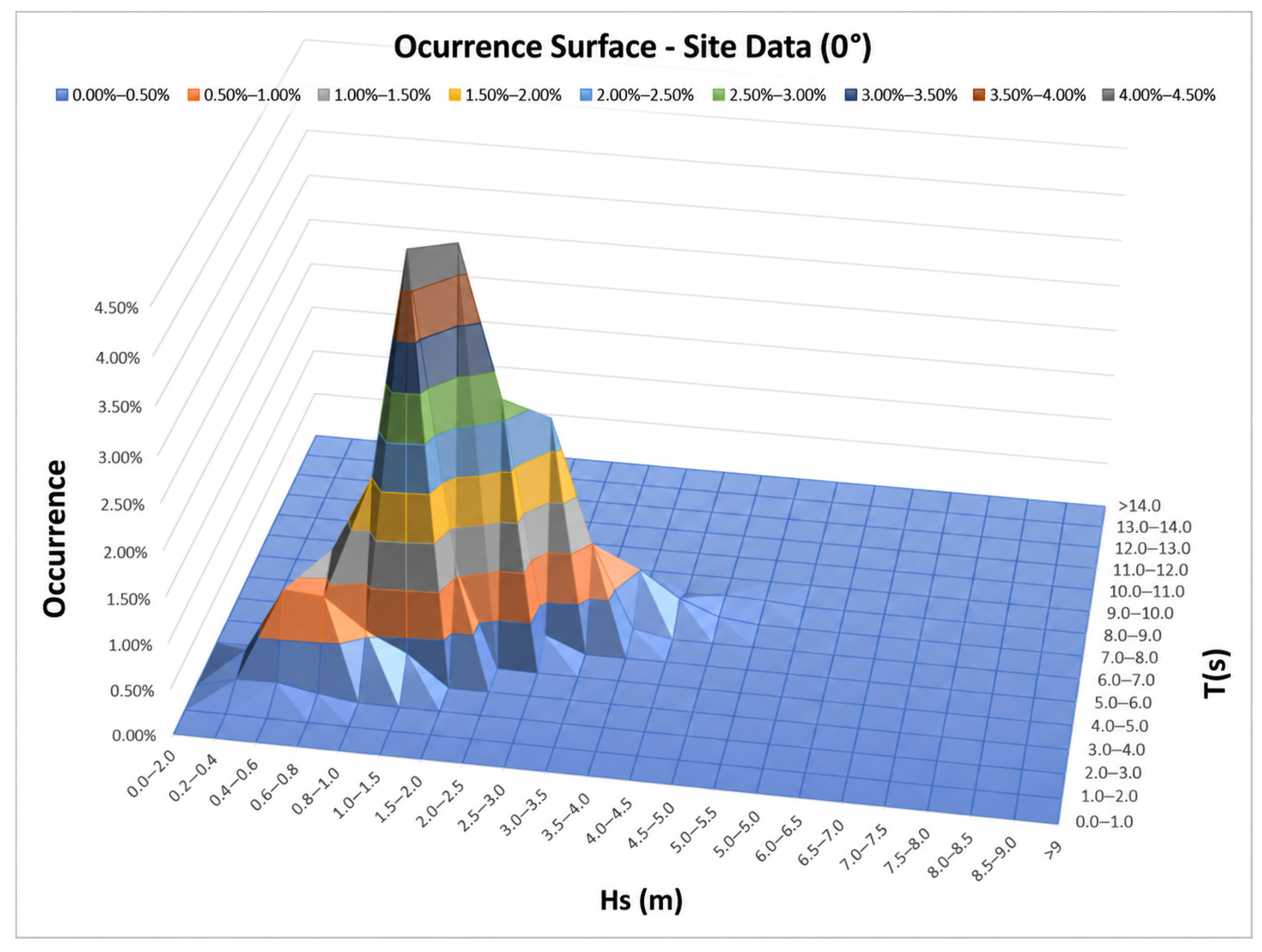
The installation site is located off the Gulf of Roses in the north-eastern Spanish Mediterranean at water depths of 120–140 m (42.126° N–42.158° N, 3.394° E–3.437° E). Its metocean conditions are characterized by a wave scatter diagram describing the joint distribution of significant wave height (Hs) and peak period (Tp). Directional probability distributions are discretized in 30° sectors. These directional probabilities are used in the long-term fatigue weighting.

Figure A1. Site metocean data used in the fatigue assessment (0° direction example).

Figure A1. Site metocean data used in the fatigue assessment (0° direction example).

Appendix A.2. Hydrodynamic Response via Transfer Functions

Hydrodynamic analyses are carried out using the panel code AQWA, producing Response Amplitude Operators (RAOs). These RAOs are used to describe the transfer of wave energy into platform motions and structural responses at various frequencies. Each frequency-domain load case corresponds to a regular-wave component, with platform responses computed for a set of wave directions, heights, and periods. A structural simulation is performed for each detail, and the transfer function is extracted. AQWA is used here for first-order potential-flow wave excitation, diffraction, and radiation. Viscous drag and other nonlinear hydrodynamic effects are not contained in these RAOs and are treated separately in the time-domain workflow.

Figure A2. Normalized structural transfer functions: (a) C1C; (b) C2P; (c) HP.

Figure A2. Normalized structural transfer functions: (a) C1C; (b) C2P; (c) HP.

Appendix A.3. Stress Response Calculation

The frequency-domain structural response was calculated using the Ansys model and local submodels described in Section 2. Wave-induced pressure fields from AQWA were transferred to the structural model. A representative hot-spot stress range was obtained for each regular-wave block from its cyclic response. The stress range and the block height, period, direction and 25-year cycle count define the inputs to the local S–N damage calculation. The transfer-function plots describe the linear response; no stress-spectrum reconstruction was required for the block counts.

Appendix A.4. Method A for Effective Stress Extraction

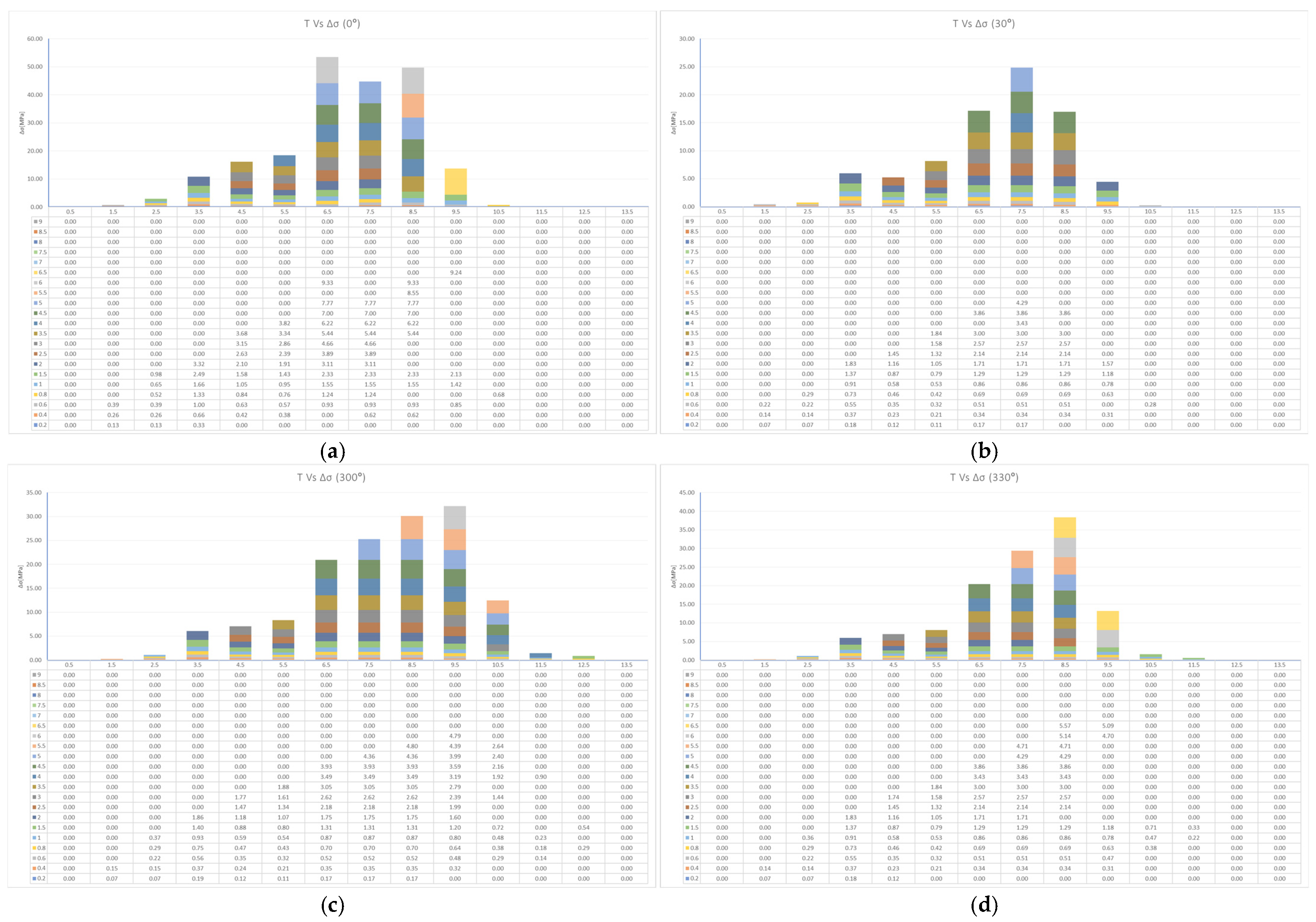
The derivation of structural hot-spot stress (Method A) [20] uses stress results extracted at 0.5t and 1.5t from the weld toe (or shell-intersection line), where t is the plate thickness. For a linear extrapolation to the weld toe, σ_hs = 1.5·σ (0.5t) − 0.5·σ (1.5t). The sampling path is taken normal to the weld toe. The extraction is accepted only after the local mesh-convergence check confirms stable hot-spot stress. The frequency-domain procedure applies this structural-stress extraction to the stress transfer functions obtained for each wave frequency and direction. Time-domain stress histories are processed separately using the Rainflow-based fatigue workflow described in Section 2.3. Figure A3 shows representative fatigue-damage histograms for detail C1C (Z1) at selected wave directions.

Figure A3. Numerical fatigue-damage histograms for detail C1C (Z1): (a) 0°; (b) 30°; (c) 300°; (d) 330°.

Figure A3. Numerical fatigue-damage histograms for detail C1C (Z1): (a) 0°; (b) 30°; (c) 300°; (d) 330°.

Appendix A.5. Fatigue-Damage Estimation

For each zone, the wave contribution is D_wave, where n_i is the number of cycles in block i over 25 years and N_i is the number of cycles to failure at its representative hot-spot stress range Δσ_i on the applicable structural S–N curve [23,20]. The occurrence duration is already included in n_i and is not applied a second time. The general Miner expression is given in Equation (A1). The turbine contribution uses the separately calculated DEL damage, with m = 4 and N_ref = 10⁷ defining the input load equivalence. Table 5 reports D_FD = D_wave + D_DEL without multiplying by DFF.

In the implemented workflow, wave damage and turbine-DEL damage are calculated separately and then added. This is a modelling approximation. Linear Miner accumulation of counted cycles does not establish that damage values calculated independently from simultaneous load components are additive. Their superposition can change the stress ranges and counted cycles. The combined result can therefore be affected by relative phase, correlation between load channels and any overlapping wave-driven content in the turbine loads. The FD damage split does not identify the dominant source of the FD–TD discrepancy. No general claim of exactness or conservatism is made for this approximation.

$$D={\displaystyle \sum _{i=1}^k}{\displaystyle \frac{n_i}{N_i}}={\displaystyle \frac{1}{a}}{\displaystyle \sum _{i=1}^k}{n}_i·{\left(∆{\sigma }_i\right)}^m$$

(A1)

References

- Li, S.; Hao, J.; Ren, Y.; Zhu, L.; Yuan, J.; Dong, Y. Numerical Modeling of a Triangle Semi-Submersible Floating Wind Platform Under Wave–Current Flows. J. Mar. Sci. Eng. 2025, 13, 714. [Google Scholar] [CrossRef] [Scilit]
- Zhong, Y.; Liu, W.; Shi, W.; Li, X.; Wang, S.; Michailides, C. Development and Optimization of a Novel Semi-Submersible Floater for Floating Wind Turbines in the South China Sea. J. Mar. Sci. Eng. 2025, 13, 1073. [Google Scholar] [CrossRef] [Scilit]
- Ma, K.T.; Huang, W.Y.; Wu, K.Y.; Ivanov, G. Wind Farm Design with 15 MW Floating Offshore Wind Turbines in Typhoon Regions. J. Mar. Sci. Eng. 2025, 13, 687. [Google Scholar] [CrossRef] [Scilit]
- Murakami, Y.; Takagi, T.; Wada, K.; Matsunaga, H. Essential Structure of S-N Curve: Prediction of Fatigue Life and Fatigue Limit of Defective Materials and Nature of Scatter. Int. J. Fatigue 2021, 146, 106138. [Google Scholar] [CrossRef] [Scilit]
- Kauzlarich, J.J. The Palmgren-Miner Rule Derived. Tribol. Ser. 1989, 14, 175–179. [Google Scholar] [CrossRef] [Scilit]
- Zhu, H.; Gao, X.; Shao, Y.; Li, K.; Zong, L.; Chen, C. Multiaxial Fatigue Behavior of EQ56 Marine High-Strength Steel under Different Strain Ratios. J. Constr. Steel Res. 2025, 227, 109368. [Google Scholar] [CrossRef] [Scilit]
- Valente, S.C.; Castello, D.A.; Ritto, T.G. Spectral Analysis of Fatigue in Drill Strings Under Torsional Vibrations. In Advances in Structural Vibration; Kurka, P., Pereira, M., Eds.; Lecture Notes in Mechanical Engineering; Springer: Cham, Switzerland, 2025; pp. 139–153. [Google Scholar] [CrossRef] [Scilit]
- Zhang, C.; Wan, R.; He, J.; Yu, J. A Multiaxial Fatigue Life Analysis Method for Automotive Components Based on LSTM-CNN. Int. J. Fatigue 2025, 199, 109062. [Google Scholar] [CrossRef] [Scilit]
- Lei, W.; Jiang, Y.; Zhang, J. Hybrid Time–Frequency Method for Vibration Fatigue Damage Analysis under Non-Stationary Non-Gaussian Random Excitation. Mech. Syst. Signal Process. 2025, 231, 112630. [Google Scholar] [CrossRef] [Scilit]
- Palmieri, M.; Slavič, J.; Cianetti, F. Fast Evaluation of Central Moments for Non-Gaussian Random Loads in Vibration Fatigue. Mech. Syst. Signal Process. 2025, 228, 112434. [Google Scholar] [CrossRef] [Scilit]
- Sgamma, M.; Barsanti, M.; Bucchi, F.; Frendo, F. Analytical Study on the Dynamic Response of Single-DOF Mechanical Systems to Stationary Non-Gaussian Random Loads. Mech. Syst. Signal Process. 2025, 232, 112694. [Google Scholar] [CrossRef] [Scilit]
- Muñiz-Calvente, M.; Álvarez-Vázquez, A.; Pelayo, F.; Aenlle, M.; García-Fernández, N.; Lamela-Rey, M.J. A Comparative Review of Time- and Frequency-Domain Methods for Fatigue Damage Assessment. Int. J. Fatigue 2022, 163, 107069. [Google Scholar] [CrossRef] [Scilit]
- Abdelmoteleb, S.E.; Bachynski-Polić, E.E. A Frequency-Domain Optimization Procedure for Catenary and Semi-Taut Mooring Systems of Floating Wind Turbines. Mar. Struct. 2025, 101, 103768. [Google Scholar] [CrossRef] [Scilit]
- Shin, Y.H.; Lee, S.J.; Lee, M.J. Frequency-Domain Multi-Dynamic Analysis Using Response-Based Approach for FOWT. J. Ocean Eng. Technol. 2025, 39, 177–188. [Google Scholar] [CrossRef] [Scilit]
- Knezevic, D.; Pinguet, R.; Martin, B.; Peterson, J.; Podskarbi, M.; Price, S.; Vallaghe, S. Validation of a Fully Integrated Numerical Simulation Method to Assess Structural Integrity on a Flexible Model of FOWT Using RB-FEA. In Proceedings of the ASME 2022 4th International Offshore Wind Technical Conference, Boston, MA, USA, 7–8 December 2022. Paper IOWTC2022-94295. [Google Scholar] [CrossRef] [Scilit]
- Hive Wind Energy. HiveWind. Available online: https://hivewindenergy.com/ (accessed on 1 August 2026).
- Wind Turbine Models. MingYang MySE11-230 Offshore. Available online: https://en.wind-turbine-models.com/turbines/2286-mingyang-myse11-230-offshore (accessed on 26 October 2026).
- MingYang Smart Energy. Wind Turbines. Available online: https://mingyang.com/products/ (accessed on 26 October 2026).[Green Version]
- Akselos. Wind Power. Available online: https://akselos.com/wind-power/ (accessed on 26 October 2026).
- DNV-RP-C203; Fatigue Design of Offshore Steel Structures. DNV: Høvik, Norway, 2024.
- IEC 61400-1; Wind Turbines—Part 1: Design Requirements. IEC: Geneva, Switzerland, 2005.
- Arnold, D.N.; Madureira, A.L.; Zhang, S. On the Range of Applicability of the Reissner-Mindlin and Kirchhoff-Love Plate Bending Models. J. Elast. 2002, 67, 171–185. [Google Scholar] [CrossRef] [Scilit]
- Ding, J.; Chen, H.; Liu, X.; Rashed, Y.F.; Fu, Z. Fatigue Reliability Analysis of Offshore Wind Turbines Under Combined Wind–Wave Excitation via Direct Probability Integral Method. J. Mar. Sci. Eng. 2025, 13, 506. [Google Scholar] [CrossRef] [Scilit]
Disclaimer/Publisher’s Note: The statements, opinions and data contained in all publications are solely those of the individual author(s) and contributor(s) and not of MDPI and/or the editor(s). MDPI and/or the editor(s) disclaim responsibility for any injury to people or property resulting from any ideas, methods, instructions or products referred to in the content. |
© 2026 by the authors. Licensee MDPI, Basel, Switzerland. This article is an open access article distributed under the terms and conditions of the Creative Commons Attribution (CC BY) license.