Sound-Speed Inversion and LFM Layer-Drift Discrimination in Thin Sediments Based on Interference-Phase Self-Consistency

Abstract

Pulse compression in broadband linear-frequency-modulated (LFM) sub-bottom profiling suffers from coherent sidelobe coupling, causing peak-position displacement (layer drift) and pseudo-layers in thin sediments. For a low-impedance soft-mud upper layer, the interface echo also undergoes a π phase reversal, distorting envelope-based interpretation. We propose a thin-sediment sound-speed inversion and LFM layer-drift discrimination method based on interference-phase self-consistency. Using a self-developed high-frequency sub-bottom profiling sonar (HF-SSBP; 110 kHz center frequency, 30 kHz bandwidth), stepped-frequency measurements were performed from 95 to 125 kHz at 1 kHz intervals, and the interference amplitude in the overlap region of upper- and lower-interface echoes was extracted. The oscillation period and peak–trough phase encode layer thickness and sound speed and, unlike the LFM envelope, are unaffected by pulse-compression sidelobes. With thickness constrained by geometry, the LFM sound speed served as an initial reference for inversion, and LFM layer drift was diagnosed via a half-wavelength phase-error criterion. Water-tank tests on soft-mud–sand bilayers showed good agreement for Sample 2 (interference 1167 m/s; LFM 1152 m/s), confirming the two-layer interpretation, whereas Sample 3 gave 1281.69 m/s (LFM) versus 1098 m/s (interference), revealing substantial LFM drift. The π phase reversal must be explicitly modeled, with peak–trough inversion directly indicating a low-impedance zone. The method enables accurate sound-speed inversion and robust LFM layer-drift diagnosis in thin sediments.

1. Introduction

Surficial sediments constitute one of the most active boundary layers for material cycling and engineering activities in marine and nearshore aquatic environments [1,2,3]. Their layered architecture exerts a direct control on seabed geological evolution and engineering-environmental properties, making high-resolution characterization of sedimentary layering an increasingly important objective in shallow-sediment acoustics [4]. Non-contact sonar sensing can continuously acquire acoustic information without disturbing the sediment body and therefore offers both non-destructive measurement and high vertical resolution [5,6].

Among non-contact acoustic techniques, sub-bottom profilers are widely used to investigate shallow sedimentary structures because of their high vertical resolution and ability to continuously delineate stratigraphic interfaces. Representative studies include the work of Li et al., who used sub-bottom profiling data to construct an amplitude-variation-based stratigraphic model through characteristic-layer extraction [7]; Reis et al., who estimated the accumulation rate of muddy sediments in reservoirs from sub-bottom profiles [8]; and Wang et al., who quantified the thickness of modern tidal deposits by identifying shallow layers near an estuary [9]. These studies demonstrate that sub-bottom profiling can provide reliable qualitative and semi-quantitative information on layer geometry and thickness. However, measurement accuracy has received comparatively limited attention, restricting the use of this technique for fine-scale structural characterization.

Accurate characterization of layered sediments ultimately depends on reliable inversion of sediment physical properties, among which sound speed is one of the most fundamental parameters because its uncertainty directly affects the reliability of layer identification. Sound speed in shallow sediments is commonly measured using travel-time methods, in which acoustic propagation time is determined from automatically identified echo features such as first-break onset; this remains a classical approach for in situ sound-speed measurement [10]. At the same time, travel-time inversion is governed by the strong physical coupling between layer thickness and sound speed, which generally prevents the two parameters from being independently determined [11]. A range of methods has therefore been developed for sound-speed and geoacoustic inversion. Christopher et al. extracted the relative arrival-time difference between seabed and sub-bottom reflections from pulsed echoes, enabling two-layer structures on the scale of hundreds of meters to be resolved and layer sound speeds to be estimated, although the low operating frequency limited the accuracy of structural characterization [12]. Zhang et al. used high-frequency LFM signals for acoustic-impedance inversion constrained by borehole calibration, thereby recovering impedance trends and indirectly inferring sound-speed variations, but with limited capability for resolving thin layers [13]. Lima et al. converted sub-bottom profiler (SBP) envelope amplitudes into acoustic impedance using a log-linear model calibrated with MSCL-S measurements for shallow geotechnical characterization, yet thin sand and silt beds remained difficult to resolve because of vertical-resolution limitations [14]. Broadband multifrequency data combined with normal-mode modeling [15], parabolic-equation approaches [16], or near-field self-attention mechanisms [17] can improve the accuracy and efficiency of sound-speed and geoacoustic inversion, but their performance remains constrained by the resolution and signal-to-noise ratio imposed by the adopted signal architecture.

Sub-bottom profilers commonly employ broadband LFM signals followed by pulse compression to achieve high vertical resolution. Pulse compression, however, is fundamentally a coherent superposition of reflections from different interfaces in the time domain. When the echo from a deeper interface is relatively weak and its main lobe lies close in time to a sidelobe of the stronger upper-interface echo, the sidelobe can distort the weak main lobe, shifting the apparent peak position (layer drift) or generating a spurious peak (pseudo-layer) [18]. Various strategies have been proposed to mitigate sidelobe leakage and resolution limitations. Fan et al. suppressed cross-correlation-induced sidelobes by exploiting frequency-domain differences [19], whereas Zhang et al. achieved high-resolution inversion of shallow seabed structure using waveform-library constraints [20]. Nevertheless, sidelobe leakage continues to undermine the robustness of LFM envelope peaks as indicators of true interface position and therefore limits quantitative sediment interpretation. This issue is particularly important for centimeter- to decimeter-scale thin layers, such as redox horizons, where tuning interference can create imaging artifacts or even lead to erroneous layer identification [21]. The resolvable spacing of layered acoustic-impedance inversion is likewise constrained by resolution [22], although thickness modeling constrained by spectral decomposition can improve discrimination near the resolution limit [23]. Thin-layer identification methods based on optimal-basis wavelet transforms of wedge models [24], multiscale sedimentary-cycle analysis using time–frequency attributes [25], and seismic-sedimentological facies prediction [26] have also been proposed. Collectively, these studies show that thin-bed characterization can exploit time–frequency or interference information, but they do not fundamentally remove sidelobe coupling inherent to LFM pulse compression.

A further complication arises when the surficial layer consists of highly porous soft or fluid mud containing microbubbles. In such cases, both sound speed and acoustic impedance may fall below those of the overlying water, forming a characteristic low-acoustic-impedance (reverse-polarity) zone [27,28]. The reflection coefficient at such an interface is negative, and the reflected waveform undergoes a π phase reversal, in contrast to the conventional positive-polarity assumption [29]. Most existing echo-processing approaches for thin sediments implicitly assume positive polarity and rarely account for this reverse-polarity condition. If the phase reversal is ignored, layer identification and sound-speed inversion based on envelope peak position or interference phase can incur substantial systematic errors.

In summary, fine-scale characterization of shallow sedimentary layers is constrained by both the sensing modality and the inversion strategy. Our group has developed a high-frequency sub-bottom profiling sonar (HF-SSBP) for acoustic investigation of surficial sediments. Previous deployments in the deep South China Sea confirmed the presence of centimeter-scale shallow layering [30] and enabled measurements of sound speed, extraction of reflection coefficients, and acoustic sediment classification [31,32,33]. These studies, however, were still based on the LFM operating mode of the HF-SSBP and therefore remained susceptible to pulse-compression sidelobe leakage and to π phase reversal in low-impedance layers. To overcome these limitations, the present study extends the signal modality while retaining the existing hardware. The HF-SSBP transmits a broadband LFM waveform with a center frequency of 110 kHz and a bandwidth of 30 kHz and uses coherent reception with high amplitude-and-phase fidelity. This architecture allows the transmitted waveform to be flexibly modified without changing the acoustic hardware. We therefore implemented a stepped-frequency mode spanning 95–125 kHz in 1 kHz increments and recorded the echo at each frequency, using the frequency-dependent oscillation of the interference amplitude to complement LFM-based acoustic-parameter inversion and layer discrimination.

Specifically, we combine stepped-frequency interference amplitudes with LFM measurements for layer identification and sound-speed inversion. The oscillation period and peak–trough phase of the frequency-domain interference response provide identifiable quantities that are sensitive to layer thickness and sound speed, respectively, and are used to diagnose layer drift and pseudo-layer arising from LFM pulse compression. Meanwhile, explicit correction for the π phase reversal of the upper-interface echo enables high-accuracy inversion of the upper layer sound speed. By exploiting the coherent amplitude-and-phase fidelity of the HF-SSBP, the proposed approach extends the measurement dimension from time-domain envelope imaging to quantitative frequency-dependent interference analysis. Water-tank experiments and numerical simulations using soft-mud–sand bilayer samples are used to validate the method. The results show that interference-amplitude information can effectively diagnose LFM layer drift and pseudo-layer in thin low-impedance sediments, improve upper layer sound-speed estimation, and provide a practical means of identifying and characterizing low-acoustic-impedance zones.

2. Theoretical Framework

2.1. Two-Layer Structure by LFM Compression

The HF-SSBP transmits a broadband LFM signal. Let the carrier frequency be f_c and the bandwidth be B. The transmitted waveform can be written as

$$s_1(t)=\mathit{rect}({\displaystyle \frac{t}{T}})e^{j2\pi (f_{c}t+{\displaystyle \frac{K}{2}}{t}^2)}, \mathrm{while} \mathit{rect}({\displaystyle \frac{t}{T}})=\left\{\begin{array}{l}1,\left|{\displaystyle \frac{t}{T}}\right|\le 1\\ 0,\mathrm{elsewise}\end{array}\right.$$

(1)

where K = B/T is the chirp rate and T is the pulse duration. For the two-layer sediment considered here, consisting of an upper mud layer overlying sand, let the distance from the transducer aperture to the upper sediment surface be R₁ and let the upper layer thickness be D₀. The received echo from the two-layer sediment can then be expressed as

$$\left\{\begin{array}{c}{s}_{r1}(t)=A_1\mathit{rect}({\displaystyle \frac{t-{\tau }_1}{T}})e^{j2\pi (f_c(t-{\tau }_1)+{\displaystyle \frac{K}{2}}{(t-{\tau }_1)}^2)}+A_2\mathit{rect}({\displaystyle \frac{t-{\tau }_2}{T}})e^{j2\pi (f_c(t-{\tau }_2)+{\displaystyle \frac{K}{2}}{(t-{\tau }_2)}^2)}\hfill \\ {\tau }_1={\displaystyle \frac{2R_1}{c_w}},{\tau }_2={\displaystyle \frac{2R_1}{c_w}}+{\displaystyle \frac{2D_0}{c_{s1}}}\hfill \end{array}\right.$$

(2)

where c_w and c_s1 denote the sound speeds in water and in the upper sediment layer, respectively, and A₁ and A₂ denote the amplitudes of the reflections from the upper and lower interfaces, respectively. The matched filter for the LFM signal is the time-reversed complex conjugate of the transmitted waveform, h(t) = s^*(−t). Applying this filter to the received echo yields the pulse-compressed signal s_o(t), given by

$$\begin{array}{cc}\hfill s_{o1}(t)=& s_r(t)*h(t)\hfill \\ \hfill =& {\displaystyle {\displaystyle \underset{-\infty }{\overset{\infty }{\int }}}\left[A_1\mathit{rect}(\frac{u-{\tau }_1}{T})e^{j2\pi (f_c(u-{\tau }_1)+\frac{K}{2}{(u-{\tau }_1)}^2)}+A_2\mathit{rect}(\frac{u-{\tau }_2}{T})e^{j2\pi (f_c(u-{\tau }_2)+\frac{K}{2}{(u-{\tau }_2)}^2)}\right]h(t-u)\mathit{du}}\hfill \\ \hfill =& A_{1}T{\displaystyle \frac{\mathit{sin\pi KT}(1-\frac{\left|t-{\tau }_1\right|}{T})t}{\mathit{\pi KT}(\left|t-{\tau }_1\right|)}}\mathit{rect}({\displaystyle \frac{\left|t-{\tau }_1\right|}{2T}})e^{j2\pi f_c(\left|t-{\tau }_1\right|)}+A_{1}T{\displaystyle \frac{\mathit{sin\pi KT}(1-\frac{\left|t-{\tau }_2\right|}{T})t}{\mathit{\pi KT}(\left|t-{\tau }_2\right|)}}\mathit{rect}({\displaystyle \frac{\left|t-{\tau }_2\right|}{2T}})e^{j2\pi f_c(\left|t-{\tau }_2\right|)}\hfill \\ \hfill \approx & A_1\mathit{TSa}\left[\mathit{\pi B}(t-{\tau }_1)\right]\mathit{rect}({\displaystyle \frac{t-{\tau }_1}{2T}})e^{j2\pi f_c(\left|t-{\tau }_1\right|)}+A_2\mathit{TSa}\left[\mathit{\pi B}(t-{\tau }_2)\right]\mathit{rect}({\displaystyle \frac{t-{\tau }_2}{2T}})e^{j2\pi f_c(\left|t-{\tau }_2\right|)}\hfill \end{array}$$

(3)

Equation (3) extends the classical LFM pulse-compression formulation to a two-layer sediment. The width of the Sa(·) function defines the temporal resolution δt, which is determined by the bandwidth, i.e., δt = 1/B. Because the HF-SSBP employs a broadband LFM signal, its time–bandwidth product satisfies TB ≫ 1, which implies T ≫ δt. Under this condition, truncation of Sa(·) by the rect(·) window in Equation (3) can be neglected, yielding

$$\begin{array}{ll}\hfill s_{o1}(t)\Rightarrow & A_1\mathit{TSa}\left[\mathit{\pi B}(t-{\tau }_1)\right]e^{-j2\pi f_c{\tau }_1}+A_2\mathit{TSa}\left[\mathit{\pi B}(t-{\tau }_2)\right]e^{-j2\pi f_c{\tau }_2}\hfill \\ \hfill \Rightarrow & e^{-j2\pi f_c{\tau }_1}\left\{A_1\mathit{Sa}\left[\mathit{\pi B}(t-{\tau }_1)\right]+A_2\mathit{Sa}\left[\mathit{\pi B}(t-{\tau }_2)\right]e^{-j2\pi f_c\Delta \tau }\right\},\mathrm{while} \Delta \tau ={\displaystyle \frac{2D_0}{c_s}}\hfill \end{array}$$

(4)

Equation (4) shows that the two-layer sediment echo can be interpreted as the coherent superposition of two Sa(·)-shaped echo components. The composite waveform is jointly controlled by the amplitudes of the upper- and lower-interface echoes, their interface-dependent delays, and the layer-thickness-dependent phase difference. When the sidelobe of a strong echo distorts the main lobe of a weaker echo, the pulse-compressed peak associated with the weak interface is displaced, producing layer drift. In addition, constructive superposition of sidelobes from the two echoes can elevate sidelobe energy and generate spurious extrema, which may be misinterpreted as additional layers.

2.2. Stepped-Frequency Interference

Removing the chirp term ${\displaystyle \frac{1}{2}}K{t}^2$ from Equation (1), the waveform can be rewritten as a single-frequency signal of finite duration:

$$s_2(t)=\mathit{rect}({\displaystyle \frac{t}{T}})e^{j2\mathit{\pi ft}},f\in \left[f_c-{\displaystyle \frac{B}{2}},f_c+{\displaystyle \frac{B}{2}}\right]$$

(5)

Substituting this waveform into the same two-layer sediment model gives the received echo as

$$\begin{array}{cc}\hfill s_{r2}(t)=& A_1\mathit{rect}({\displaystyle \frac{t-{\tau }_1}{T}})e^{j2\mathit{\pi f}(t-{\tau }_1)}+A_2\mathit{rect}({\displaystyle \frac{t-{\tau }_2}{T}})e^{j2\mathit{\pi f}(t-{\tau }_2)}\hfill \\ \hfill =& e^{j2\mathit{\pi f}(t-{\tau }_1)}\left[A_1\mathit{rect}({\displaystyle \frac{t-{\tau }_1}{T}})+A_2\mathit{rect}({\displaystyle \frac{t-{\tau }_2}{T}})e^{-j2\mathit{\pi f}\Delta \tau }\right]\hfill \end{array}$$

(6)

Taking the amplitude of the received echo gives

$$\left|s_{r2}(t)\right|=\sqrt{A_1^2\mathit{rect}({\displaystyle \frac{t-{\tau }_1}{T}})+A_2^2\mathit{rect}({\displaystyle \frac{t-{\tau }_2}{T}})+2A_1{A}_2\mathit{rect}({\displaystyle \frac{t-{\tau }_1}{T}})\mathit{rect}({\displaystyle \frac{t-{\tau }_2}{T}})\cos (2\mathit{\pi f}\Delta \tau )}$$

(7)

Restricting the analysis to the overlap region of the upper- and lower-interface echoes, Equation (7) reduces to

$$\left\{\begin{array}{c}\left|{\tilde{s}}_{r2}(t)\right|=\sqrt{A_1^2+A_2^2+2A_1{A}_2\cos (\Delta \varphi )},t\in \left[{\tau }_2-{\displaystyle \frac{T}{2}},{\tau }_1+{\displaystyle \frac{T}{2}}\right]\hfill \\ \Delta \varphi ={\displaystyle \frac{4\pi D_0}{c_{s1}}}f\hfill \end{array}\right.$$

(8)

Equation (8) shows that the oscillatory behavior in the interference overlap region of the upper- and lower-interface echoes is governed entirely by cos(Δϕ). Thus, for fixed layer thickness D₀ and sound speed c_s1, the response depends only on frequency f. Consequently, within the HF-SSBP bandwidth, stepping the transmit frequency f produces a periodically oscillating interference amplitude, whose oscillation period is linked to sediment-layer thickness and sound speed.

2.3. Phase-Reversal Effect

To examine the case in which the acoustic impedance of the upper sediment layer is lower than that of water, we introduce the classical acoustic-reflection relation. The pressure reflection coefficient at a planar interface is defined as

$$R_z={\displaystyle \frac{Z_2-Z_1}{Z_2+Z_1}}$$

(9)

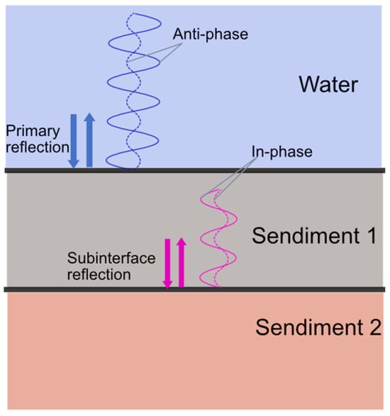
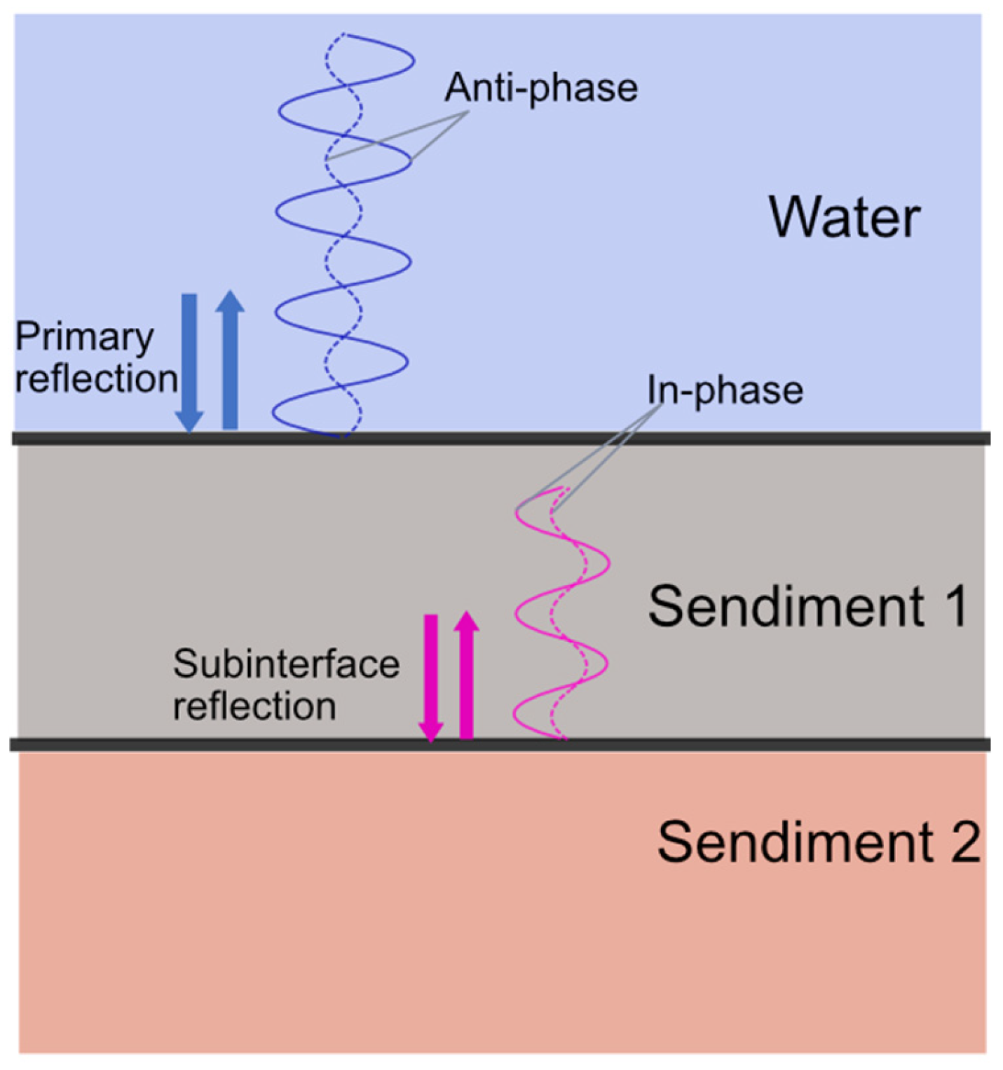
where Z₁ and Z₂ are the acoustic impedances of the incident and transmitted media, respectively. When an acoustic wave propagates from a lower-impedance medium into a higher-impedance medium, i.e., Z₂ > Z₁, the reflection coefficient satisfies R_z > 0 and the reflected phase is unchanged. Conversely, when the wave propagates from a higher-impedance medium into a lower-impedance medium, i.e., Z₂ < Z₁, the reflection coefficient satisfies R_z < 0 and the reflected wave undergoes a π phase reversal. The simplified two-layer sediment model considered in this study is shown in Figure 1. For a low-acoustic-impedance upper sediment layer, the reflection from the water–sediment-1 interface undergoes a π phase reversal, whereas the reflection from the lower interface, where the wave encounters a higher-impedance medium, retains its phase. Consequently, the upper- and lower-interface echoes received by the HF-SSBP differ in phase by π; this phase offset cannot be neglected in phase-sensitive processing.

Figure 1. Schematic of acoustic reflections in a two-layer sediment structure.

When the upper sediment layer has a lower acoustic impedance than water, the LFM pulse-compression result in Equation (4) becomes

$$s_{o1,\mathit{rev}}(t)\Rightarrow e^{-j2\pi f_c{\tau }_1}\left\{-\left|A_1\right|\mathit{Sa}\left[\mathit{\pi B}(t-{\tau }_1)\right]+\left|A_2\right|\mathit{Sa}\left[\mathit{\pi B}(t-{\tau }_2)\right]e^{-j2\pi f_c\Delta \tau }\right\}$$

(10)

Comparison of Equations (4) and (10) shows that a low-acoustic-impedance upper layer does not alter the main-lobe delay of the LFM pulse-compressed response. It does, however, change the coherent-superposition relationship between the upper- and lower-interface echoes. Consequently, the locations of layer drift and pseudo-layer produced by sidelobe interference can shift. In measured pulse-compressed waveforms, these changes are difficult to identify unambiguously; LFM pulse compression alone therefore cannot reliably determine whether phase reversal has occurred, much less quantify its effect.

For a low-acoustic-impedance upper layer, the stepped-frequency echo expression in Equation (8) is likewise modified as

$$\left|{\tilde{s}}_{r2,\mathit{rev}}(t)\right|=\sqrt{A_1^2+A_2^2+2\left|A_1\right|\left|A_2\right|\cos (\Delta \varphi +\pi )},t\in \left[{\tau }_2-{\displaystyle \frac{T}{2}},{\tau }_1+{\displaystyle \frac{T}{2}}\right]$$

(11)

Comparing Equations (8) and (11) shows that inclusion of the π phase reversal globally interchanges the peaks and troughs of the interference-amplitude-versus-frequency curve. This observable phase change has three important implications. First, it provides direct evidence that the upper layer is a low-acoustic-impedance zone. Second, it must be incorporated into the interference model to obtain an unbiased sound-speed inversion; otherwise, the optimum solution exhibits a systematic error. Third, it provides a phase prior for identifying the two-layer structure: peak–trough inversion confirms that the oscillation originates from a dual-interface configuration consisting of a low-impedance upper layer over a higher-impedance lower layer.

3. Experimental System

3.1. HF-SSBP Specifications and Waveform-Mode Extension

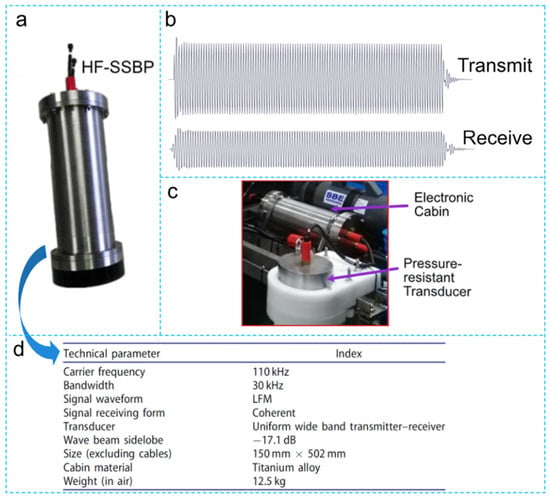
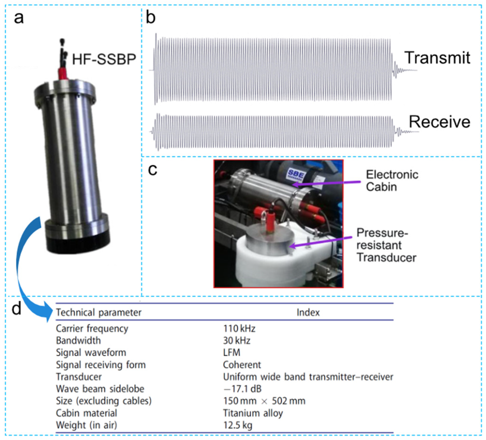
The HF-SSBP is a self-developed sonar system for high-resolution sub-bottom profiling, while the instrument is shown in Figure 2a. It transmits an LFM signal with a center frequency of 110 kHz and a 30 kHz bandwidth (95–125 kHz). The receiver uses coherent acquisition referenced to the same source as the transmitter, thereby preserving the amplitude and phase of the returned echo. Representative transmitted and received waveforms from a standard reference target are shown in Figure 2b. Depending on deployment requirements, the HF-SSBP can be operated as an integrated instrument or separated into a pressure-resistant transducer and an electronic cabin, as illustrated in Figure 2c. The system was deployed aboard the manned submersible Deep Sea Warrior during cruise TS12-01 in the deep South China Sea and completed 12 consecutive dives without failure. Additional principal technical specifications are provided in Figure 2d.

Figure 2. HF-SSBP system and its principal characteristics: (a) photograph of the developed system; (b) transmitted and received signals; (c) deployment on the Deep Sea Warrior submersible; (d) key specifications.

The primary HF-SSBP operating mode transmits a broadband LFM signal and applies pulse compression to the received echoes to produce high-resolution images of shallow sedimentary structure. To improve the detectability of thin layers, we added a stepped-frequency mode through waveform design without modifying the hardware. This mode exploits the 95–125 kHz transmit bandwidth and the coherent amplitude/phase fidelity of the system. Single-frequency signals with a pulse duration of 1 ms are transmitted sequentially at 1 kHz increments across the band, while the corresponding echoes are recorded synchronously. The interference-amplitude-versus-frequency curve is then extracted from the overlap region of the upper- and lower-interface echoes. The resulting HF-SSBP therefore supports two complementary measurement modes. The LFM mode provides a high-resolution pulse-compressed envelope for approximate interface localization and for observing layer drift and pseudo-layer, whereas the stepped-frequency mode exploits interference-phase information to accurately invert upper layer sound speed and identify low-acoustic-impedance zones; the resulting inversion is then used to validate the LFM envelope interpretation. In addition, a 110 kHz, 10-cycle burst mode is retained for system self-checks, pulse-to-pulse stability assessment, and independent sound-speed measurement.

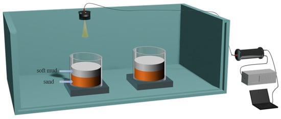
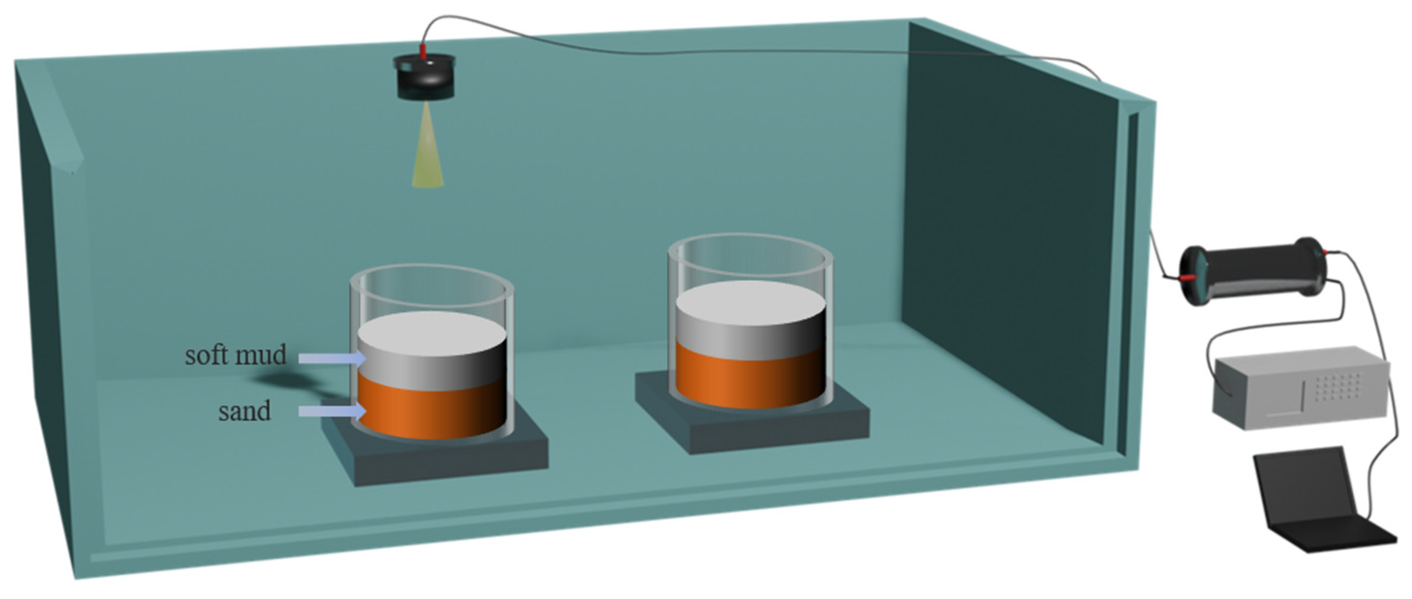
3.2. Water-Tank Experimental Setup

The measurements were conducted in a laboratory acoustic tank measuring 4 m × 2.5 m × 1.7 m. The tank floor was flat and the walls were not fitted with acoustic absorbers; the configuration is shown in Figure 3. Because the HF-SSBP transducer has a narrow beamwidth of only 5.8°, multipath reflections from the tank walls and other interfaces largely fall outside the main echo window, allowing approximately free-field measurement conditions even in the non-anechoic tank. The samples could also be stably positioned on the flat tank floor. The experimental system consisted of the HF-SSBP transducer and electronic cabin, a PC, and a DSO-X 3054A oscilloscope (Keysight Technologies, Santa Rosa, CA, USA). The PC controlled signal transmission and reception, the oscilloscope monitored echo quality in real time, and the received data were acquired by the electronic cabin and transferred to the PC for offline processing.

Figure 3. Schematic of the water-tank experimental configuration.

Two sediment samples, denoted Samples 2 and 3, were prepared with the same two-layer configuration but different mud-layer thicknesses. Each sample was contained in an acrylic cylinder with an inner diameter of 30 cm and a height of 30 cm, resting on a 10 cm thick acrylic plate. Saturated sand was first placed in the cylinder and allowed to settle; after the overlying water had been removed, a muddy sediment layer was added. During preparation of the mud, tap water was added and thoroughly mixed, after which the mixture was left to stand for 6 h and then remixed to eliminate large entrained air bubbles. Nevertheless, because dissolved gases remained in the tap water, a certain amount of fine bubbles was still retained within the mud. According to effective-medium theory for bubbly media, even a small gas fraction can substantially reduce the effective bulk modulus of the mixture, thereby decreasing both the sound speed and acoustic impedance; this preparation procedure was therefore expected to produce a stable low-acoustic-impedance mud layer, an inference subsequently supported by the measured mud sound speeds being lower than that of water. The samples were prepared in July 2025, slowly lowered to the tank floor using the positioning system, and subsequently left undisturbed in situ until the formal measurements conducted in July 2026. During this one-year period of submergence, the mud layers underwent prolonged self-weight consolidation and settlement, allowing their physical state and layer geometry to largely stabilize before acoustic testing. Immediately prior to measurement, the layer thicknesses were rechecked using a ruler in combination with an underwater camera, giving mud-layer thicknesses of 86.4 mm for Sample 2 and 91.0 mm for Sample 3.

During the formal measurements, the transducer was sequentially positioned above Samples 2 and 3. For each sample, LFM signals, stepped-frequency signals from 95 to 125 kHz, and 110 kHz 10-cycle burst signals were transmitted while the echoes were recorded synchronously. The two samples were prepared and deployed under identical conditions, and the measurement state was kept consistent to ensure direct comparability.

3.3. Measurement Procedure

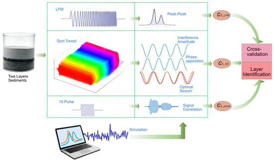
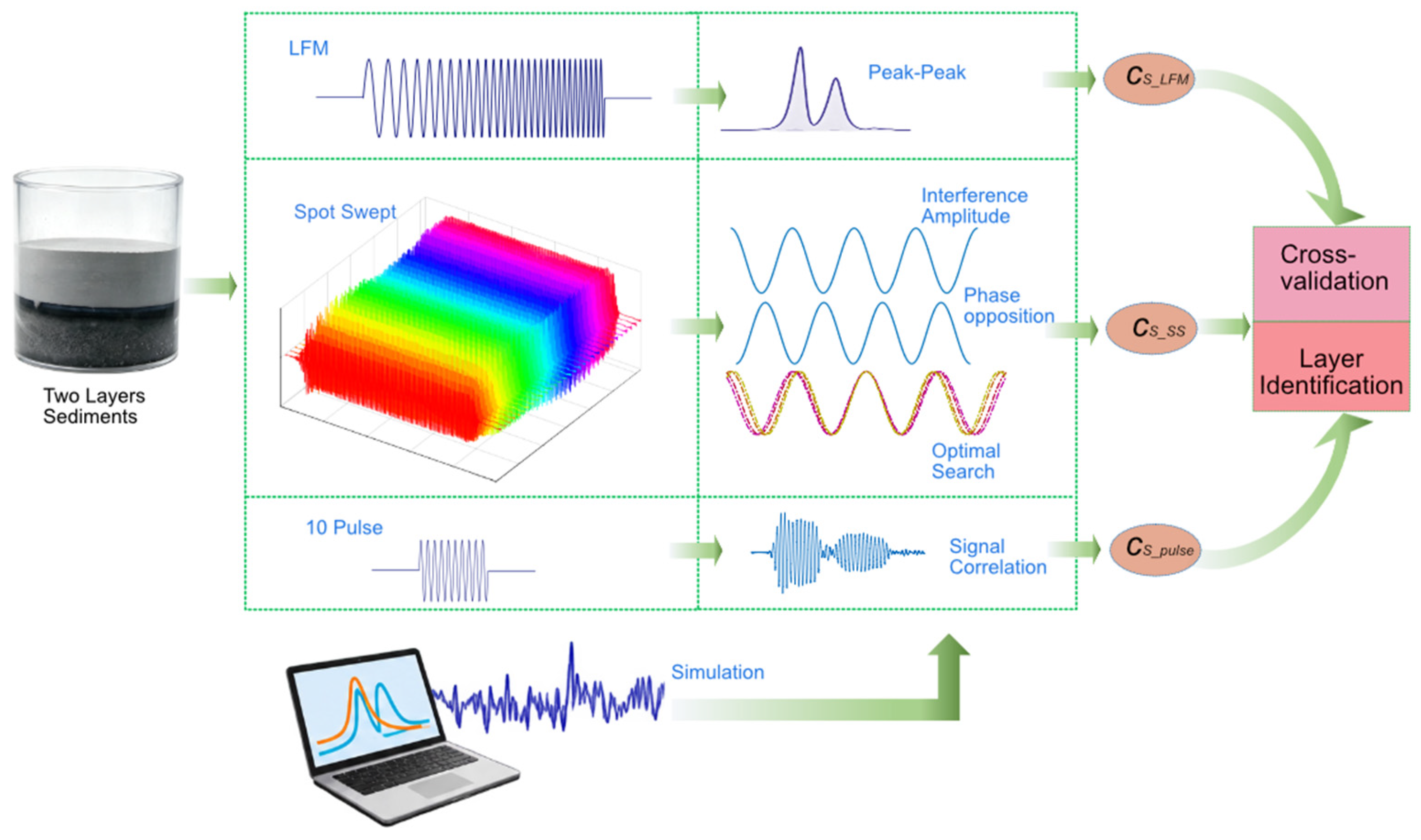
Based on the theoretical formulation in Section 2 and the experimental setup described above, laboratory measurements were performed on the two-layer sediment Samples 2 and 3. The workflow consisted of LFM measurement, stepped-frequency interference measurement, an independent burst measurement, and subsequent layer-structure diagnosis and sound-speed calibration, as summarized in Figure 4. All signal simulations and data processing in this section were implemented in Python 3.7.

Figure 4. Workflow for experimental measurements and numerical simulations.

The LFM measurement was performed first. The transducer was oriented normal to the sample surface and transmitted an LFM signal with a center frequency of 110 kHz, a bandwidth of 30 kHz, and a pulse duration of 1 ms while the echo was recorded synchronously. After pulse compression according to Equation (4), the peak delays t₁ and t₂ of the upper- and lower-interface echoes were identified, giving the delay difference Δt = t₂ − t₁. The sound speed of the upper sediment layer was then calculated as c_{S_LFM} = 2D₀/Δt.

Next, stepped-frequency interference measurements were performed. Single-frequency signals with a pulse duration of 1 ms were transmitted from 95 to 125 kHz at 1 kHz increments, and the corresponding echoes were recorded. At each frequency, the overlap interval of the upper- and lower-interface echoes was determined from the envelope evolution, and the steady-state amplitude within this interval was extracted to obtain the measured interference-amplitude-versus-frequency curve A(f_i). The layer-structure information is encoded in the interference term. The interference phase Δϕ determines the oscillation period and peak–trough positions of the cosine term in Equation (8), whereas a π phase reversal of the upper-interface echo changes the sign of the cosine term and therefore appears as an inversion of the interference oscillation phase. Simulated received echoes were used to generate interference amplitudes A′(f_i) both with and without the π reversal. After separately normalizing measured A(f_i) and simulated A′(f_i), their oscillation phases were compared, and the model whose peak and trough positions more closely matched the measurements was taken to represent the actual phase state. On this basis, a search interval was defined around c_{S_LFM}, and simulations were performed at discrete candidate sound speeds. For each candidate, the normalized simulated interference amplitude was extracted and its correlation coefficient with the normalized measured amplitude was calculated. The sound speed corresponding to the maximum correlation coefficient was defined as the optimal estimate c_{S_SS}. An independent burst measurement was also conducted using a 110 kHz signal composed of 10 cosine cycles. After compensating the upper-interface echo for the π phase offset, the inter-interface delay was extracted by correlation and the sound speed was calculated as c_{S_pusle} = 2D₀/Δt′. Together, the LFM, stepped-frequency, and burst results provided a three-way cross-validation.

Finally, layer-structure diagnosis and sound-speed calibration were performed by comparing c_{S_SS} with c_{S_LFM}. The sound-speed deviation corresponding to a half-wavelength phase error, Δc = c_{s_LFM}/(4f_cD₀), was used as the criterion. If the difference between the two sound-speed estimates was smaller than Δc, the two-layer structure inferred from LFM pulse compression was considered physically consistent, and the sound speed was further refined using the cross-validation results. If the difference was substantially larger than Δc, the LFM peak was diagnosed as having undergone layer drift or as being contaminated by a pseudo-layer. In both cases, the stepped-frequency interference inversion was used to obtain the optimal sound speed.

It should be emphasized that the proposed method does not simultaneously invert layer thickness and sound speed. Because both travel-time and interference observations depend only on the ratio D₀/c_s1(Δt = 2D₀/c_s1,Δf = c_s1/(2D₀)), the layer thickness D₀ must be supplied independently, for example from an underwater ruler, borehole information, or geological prior knowledge, before the upper layer sound speed c_s1 can be inverted. Under the Δc criterion, the method performs a self-consistency test between the sound speeds inferred from two independently measurable quantities—LFM envelope delay and interference-amplitude phase—when layer thickness is known. The objective is to determine whether interpretation of the LFM peak has been biased by sidelobe coupling, producing layer drift or a pseudo-layer, rather than to jointly determine layer thickness and sound speed.

4. Results

4.1. Simulation of LFM Layer Drift and Pseudo-Layer

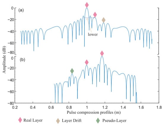
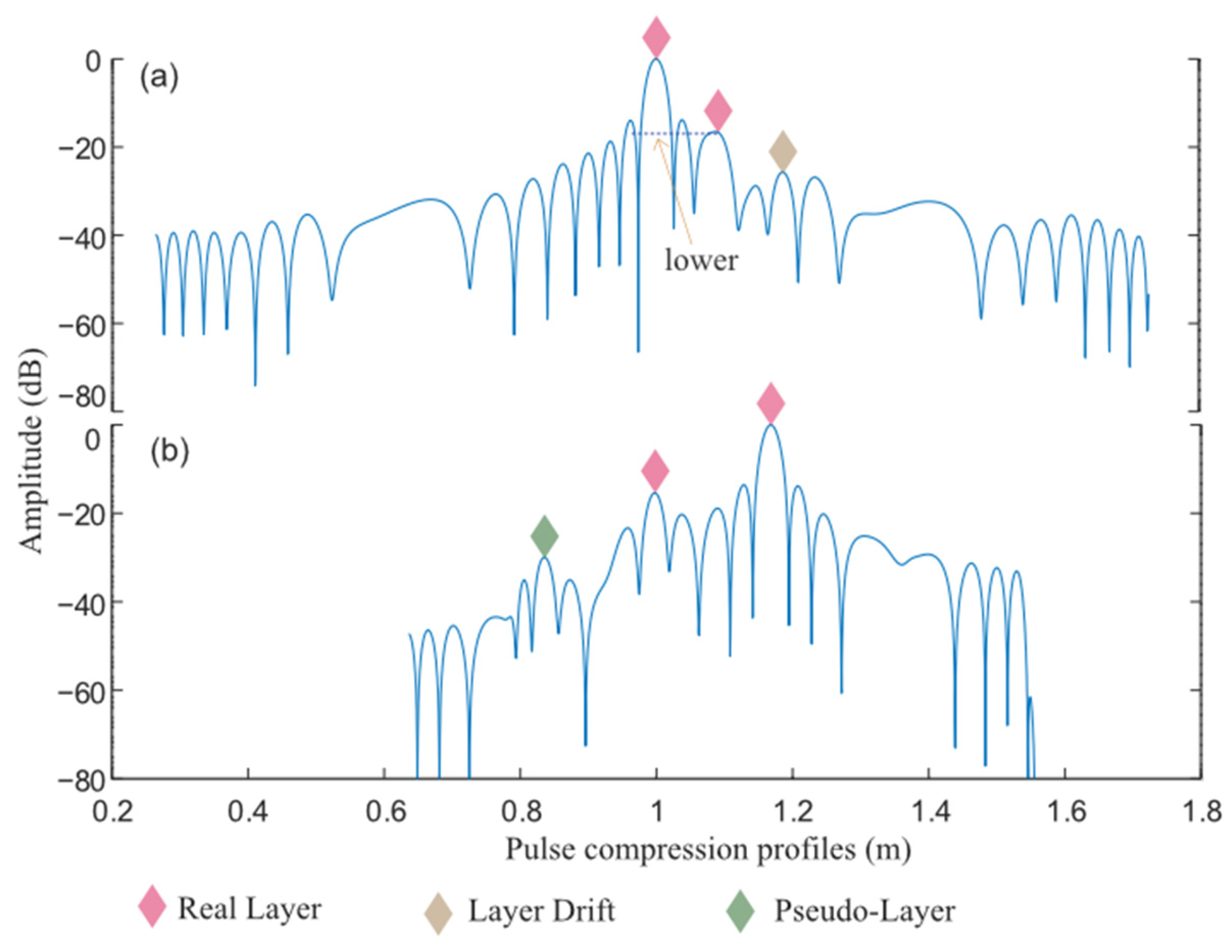
To evaluate the influence of pulse-compression sidelobes on identification of two-layer sediment structures, two representative combinations of echo-amplitude ratio and layer spacing were simulated. The center frequency was 110 kHz, the bandwidth was 30 kHz, and the medium sound speed was 1500 m/s; the time–bandwidth product satisfied the condition used in Equation (3) to neglect window truncation. The results are shown in Figure 5a,b. In Figure 5a, the interfaces are located at [1.00, 1.095] m with relative amplitudes [1.0, 0.2] and T = 1 ms. In the pulse-compressed envelope, the true main peak of the second interface falls below the sidelobe on its left, causing a spurious peak on the right to become dominant and displacing the apparent interface position; this is the layer-drift case. In Figure 5b, the two interfaces are located at [1.00, 1.17] m with relative amplitudes [0.2, 1.0] and a pulse duration T = 0.5 ms. A spurious pulse-compression maximum appears on the left, producing a false layer. These simulations demonstrate that, for particular combinations of layer spacing, amplitude ratio, and sound speed, coherent superposition between sidelobes and main lobes can generate either layer drift or pseudo-layer. Because the coupling is complex, the LFM pulse-compressed envelope alone is insufficient for reliable diagnosis, motivating the use of interference-phase information.

Figure 5. Simulation results of the double-layer structure: (a) results obtained with simulation parameter set 1; (b) results obtained with simulation parameter set 2.

4.2. Cross-Validation of the Two-Layer Structure and Sound-Speed Estimation for Sample 2

4.2.1. LFM Measurement

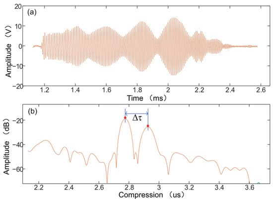
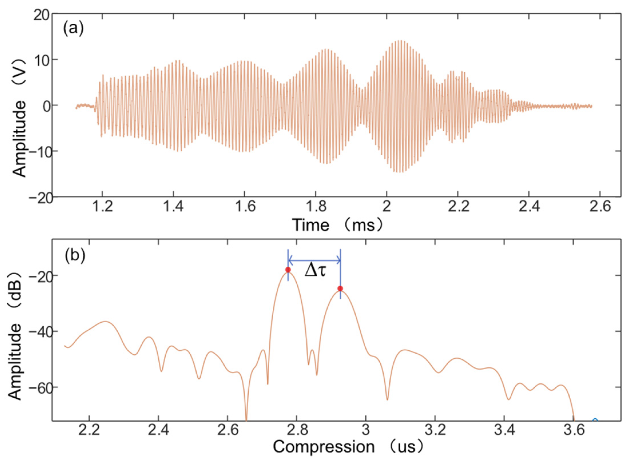
Using the experimental system described in Section 3, LFM measurements were first performed on sediment Sample 2, with the received echo and corresponding pulse-compression result shown in Figure 6. As illustrated in Figure 6a, the broadband nature of the transmitted signal causes echoes from the upper and lower interfaces to overlap and interfere irregularly in the time domain, whereas matched filtering produces two distinguishable local maxima in the pulse-compressed waveform [Figure 6b], corresponding to the two sediment interfaces. The delay between these two compressed peaks is Δt = 150 μs, substituting this value and the measured mud-layer thickness D₀ = 86.4 mm yields an estimated upper layer sound speed of c_{S_LFM} = 1152 m/s.

Figure 6. LFM pulse-compression measurement results of sediment Sample 2: (a) raw received echo; (b) pulse-compressed waveform obtained after matched filtering.

4.2.2. Measurement of Stepped-Frequency Interference

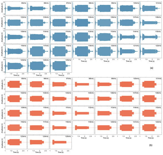
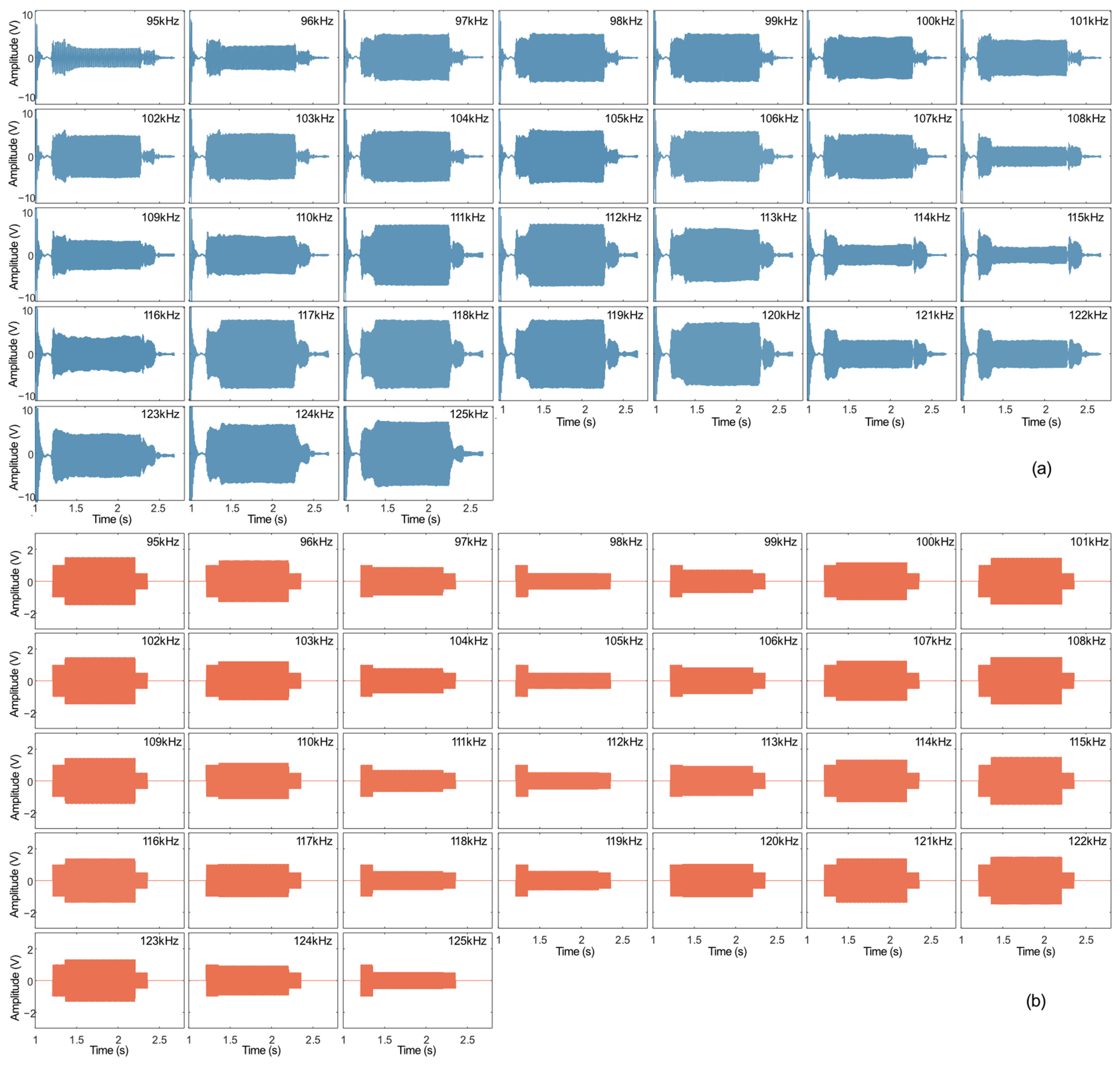
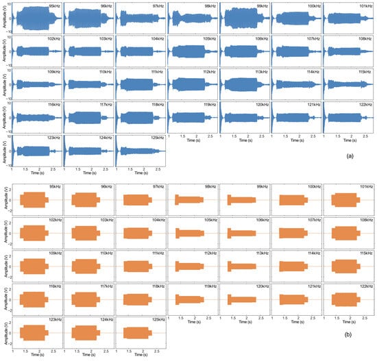
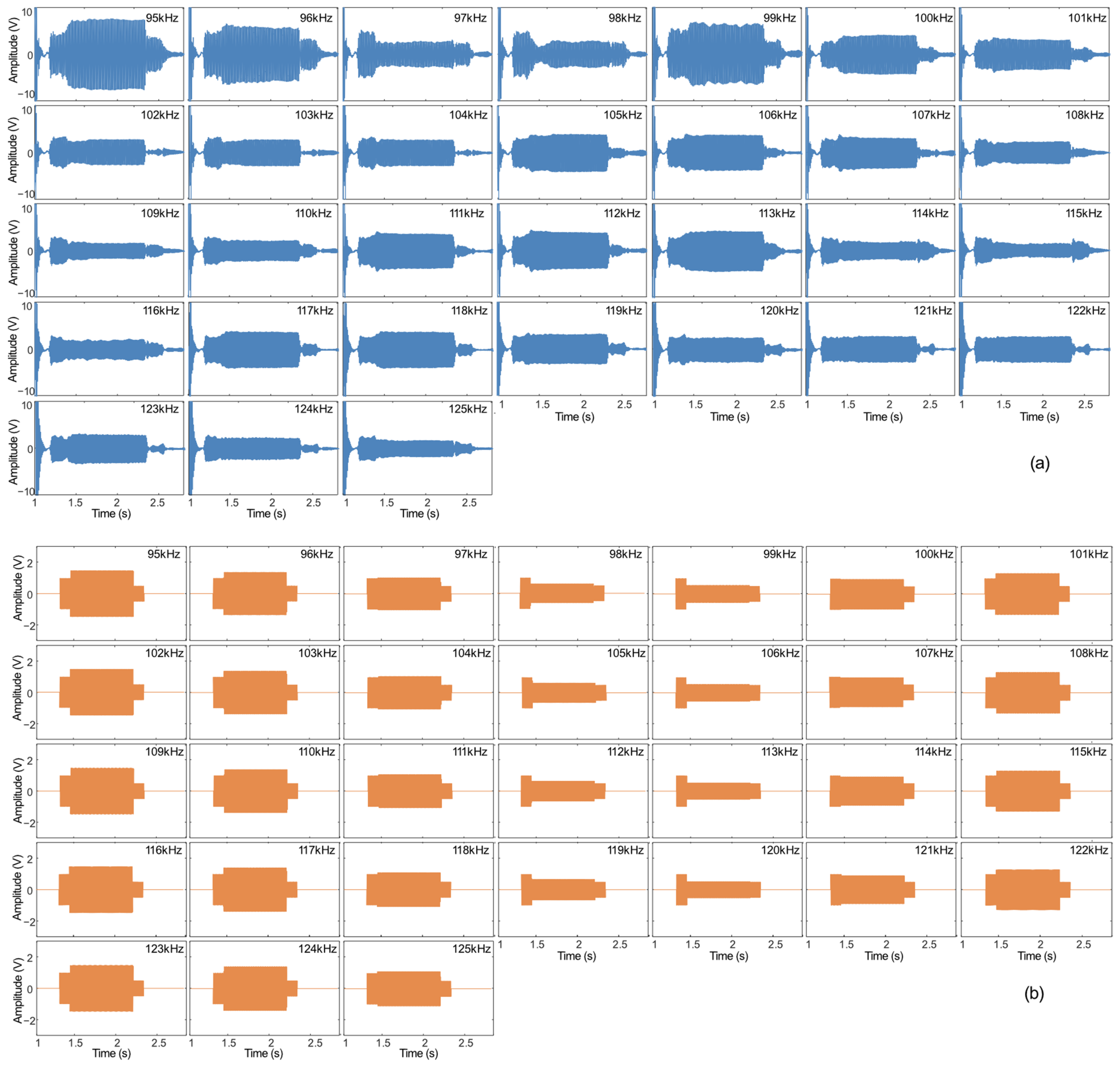
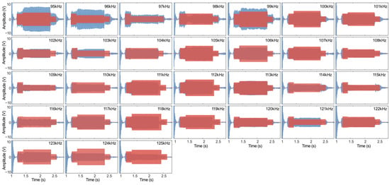
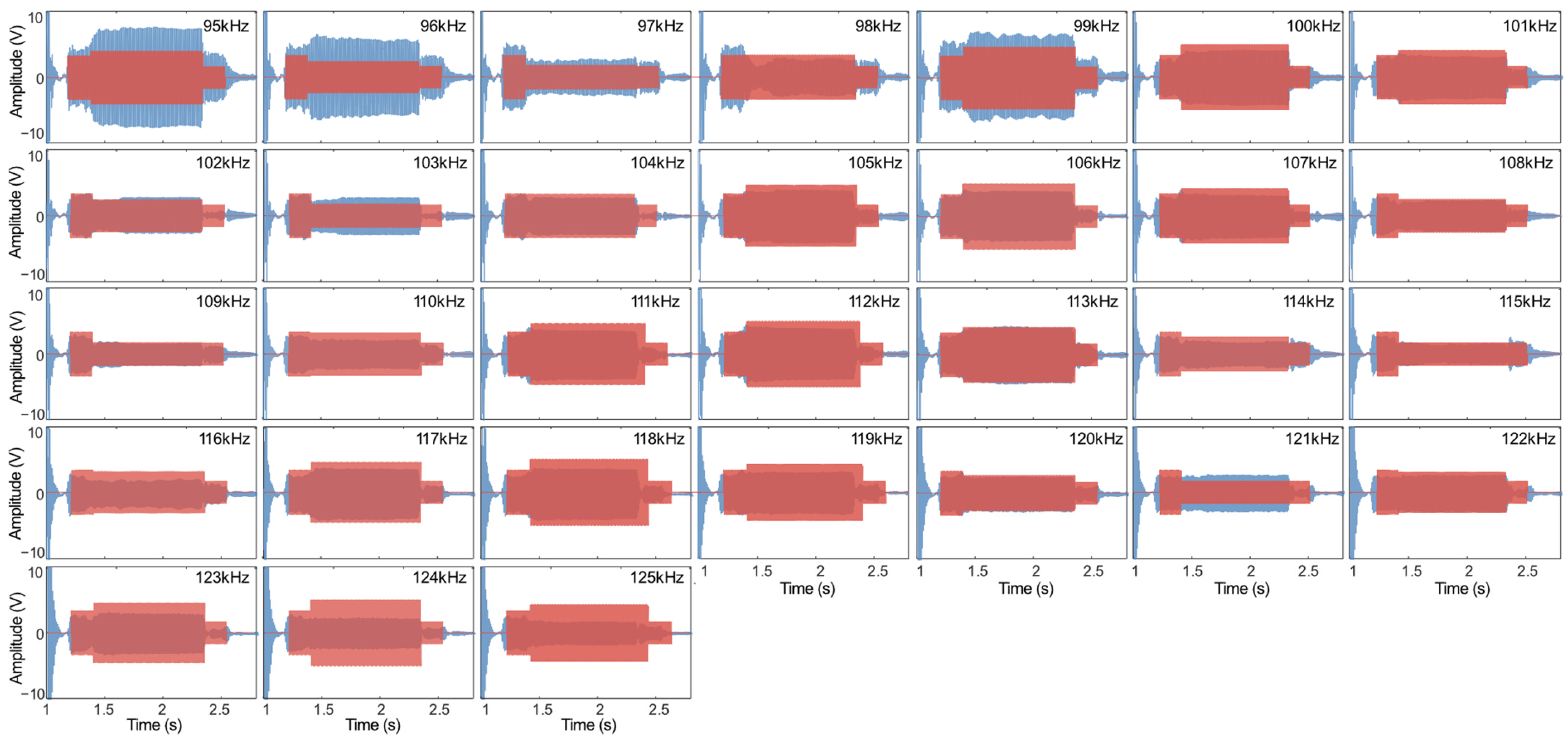
Stepped-frequency measurements were then performed on Sample 2 using frequencies from 95 to 125 kHz at 1 kHz intervals. The measured echoes are shown in Figure 7a. Echo simulations were conducted using the LFM-derived upper-layer sound speed of 1152 m/s as the reference, while all other sonar parameters were set to those of the actual HF-SSBP. The simulated echoes are shown in Figure 7b.

Figure 7. Measured and simulated stepped-frequency echoes for sediment Sample 2: (a) measured echoes; (b) simulated echoes using the LFM-derived sound speed as the reference.

Figure 8 summarizes the extraction of the interference amplitude. Figure 8a shows the interference-segment amplitudes extracted from the measured stepped-frequency echoes of Sample 2. The dashed curve denotes the unnormalized amplitude, whereas the solid curve denotes the segment-wise normalized amplitude. Normalization was applied to remove amplitude-scale differences from the phase analysis and to facilitate cross-correlation with the simulation. Figure 8b shows the corresponding interference-segment amplitudes extracted from the simulated stepped-frequency echoes. A clear opposite oscillation tendency in the interference phases is observed when the normalized curves in Figure 8a,b are compared. The simulation was therefore repeated after applying a π phase reversal to the upper-interface echo, and the corresponding interference phase was extracted, as shown in Figure 8c. The normalized curves in Figure 8a,c then exhibit a substantially more consistent oscillation trend.

Figure 8. Interference-amplitude extraction and phase-reversal verification for sediment Sample 2: (a) measured interference amplitude; (b) simulated interference amplitude without π phase reversal; (c) simulated interference amplitude with π phase reversal; (d) comparison between the measured interference curve and the simulation including π phase reversal.

The measured interference amplitudes were further compared with simulated amplitudes obtained without and with the π phase reversal using Pearson correlation coefficients. The corresponding coefficients were −0.1467 and 0.1046, respectively, indicating that the correlation changed from negative to positive after phase reversal was introduced. The absolute values of both coefficients are modest because the interference amplitude is highly sensitive to sound-speed-induced phase changes in the upper- and lower-interface echoes. Nevertheless, the relative trend agrees with the theoretical expectation. Combined with the physical observation that the LFM-derived upper layer sound speed is lower than that of water, implying an upper layer acoustic impedance below that of water and hence a negative interface reflection coefficient, the correlation comparison supports the presence of a π phase reversal in the upper-interface echo of Sample 2.

Figure 8d compares the measured interference curve with the simulation that includes the π phase reversal. The two curves exhibit the same overall phase-evolution trend, but residual amplitude and phase differences remain. This indicates that the simulation based on the LFM-derived sound speed of 1152 m/s does not fully reproduce the measurements and that the LFM estimate still contains a non-negligible error requiring further optimization.

4.2.3. Optimal Sound-Speed Inversion

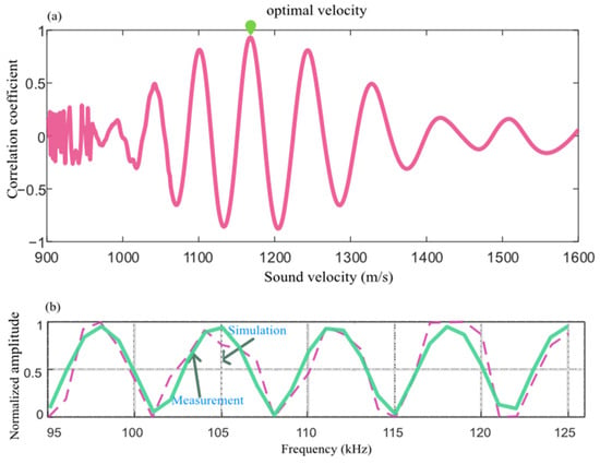
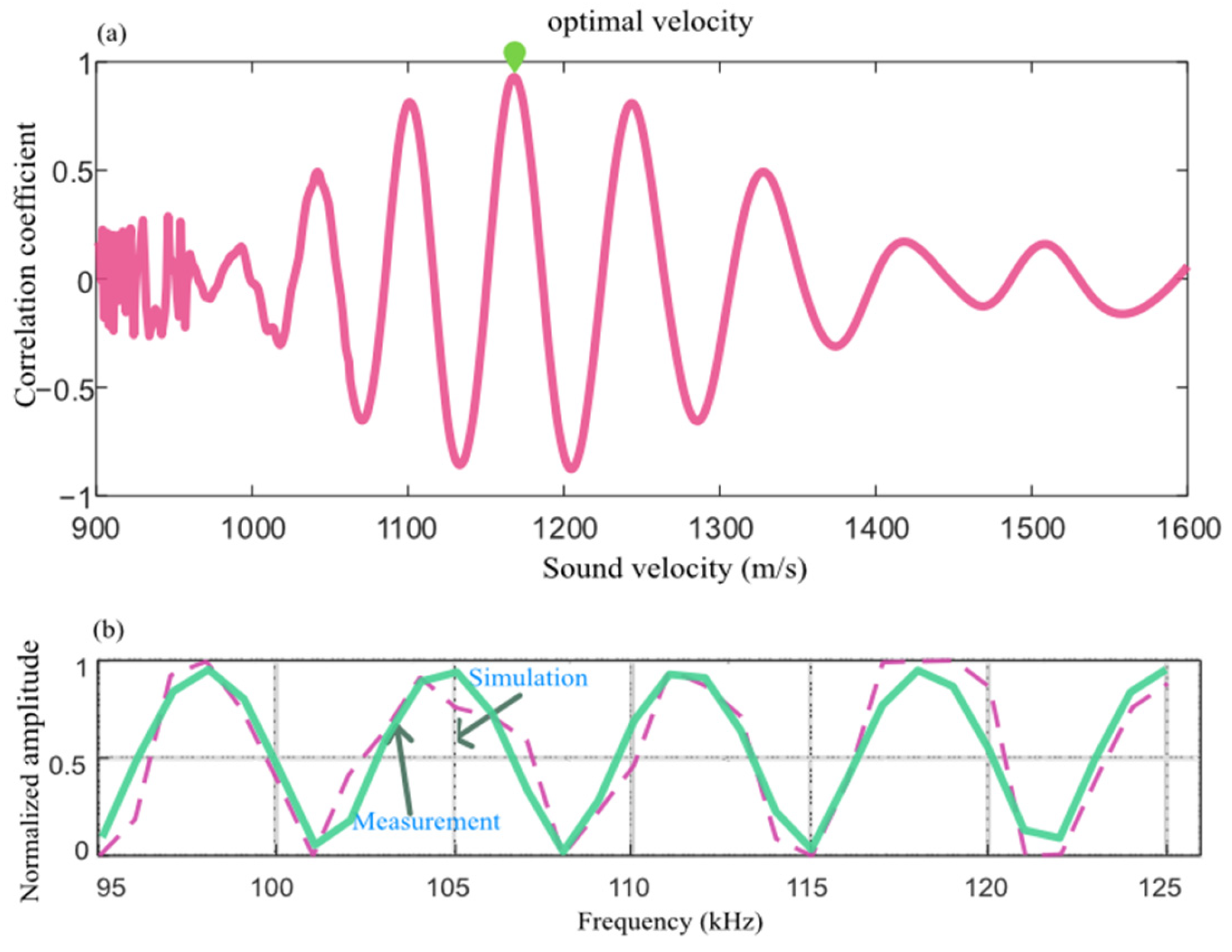
Equation (8) shows that the phase-evolution period of the interference amplitude is jointly controlled by sound speed and layer thickness. Once the layer thickness is certain, the optimal sound speed can therefore be found by simulating the two-layer echo over a range of candidate sound speeds and identifying the simulation whose interference-amplitude curve best matches the measurements. Accordingly, an optimal-sound-speed search was performed around the LFM estimate using the interval [c_{S_LFM} − 200, c_{S_LFM} + 600] m/s with a step of 1 m/s. At each candidate sound speed, the interference amplitude was simulated using the actual HF-SSBP parameters, and the Pearson correlation coefficient between the simulated and measured interference amplitudes was calculated. Figure 9a shows the correlation coefficient as a function of candidate sound speed. The sound speed at the maximum of the correlation curve was taken as the optimum, yielding c_{S_SS} = 1167 m/s. A 110 kHz burst signal consisting of 10 cosine cycles was subsequently transmitted to Sample 2. After averaging repeated echoes and compensating the upper-interface echo for the π phase offset, the inter-interface delay was estimated using correlation, giving an upper layer sound speed of c_{S_pusle} = 1163.5 m/s. Figure 9b presents a comparison between the simulated and measured interference amplitude curves under the optimal sound speed.

Figure 9. Correlation coefficient curve for optimal sound-speed inversion of sediment Sample 2: (a) correlation coefficient as a function of candidate sound speed; (b) comparison of simulated and measured interference amplitudes at the optimal sound speed.

Three sound-speed estimates were thus obtained for Sample 2: c_{S_LFM} = 1152m/s from LFM pulse compression, c_{S_SS} = 1167 m/s from stepped-frequency interference inversion, and c_{S_pusle} = 1163.5 m/s from burst correlation. The burst-correlation and stepped-frequency-interference estimates are independent measurements, and the burst result supports the plausibility of the optimal sound speed inferred from the interference method. The difference between the LFM estimate c_{S_LFM} and the interference estimate c_{S_SS} is approximately 15 m/s, which is smaller than the sound-speed deviation associated with a half-wavelength phase error (approximately 35 m/s at the 110 kHz center frequency). This agreement indicates that the two-layer structure inferred from the LFM pulse-compression response of Sample 2 is physically consistent.

Comparison of the three methods shows that LFM pulse compression provides a high signal-to-noise ratio but is affected by coherent sidelobe superposition, which limits measurement accuracy. The stepped-frequency interference method estimates sound speed from the phase of the interference amplitude and provides the highest precision, although an initial sound-speed estimate is required to constrain the search interval. The burst-correlation method extracts the time delay from the location of the correlation peak, and its robustness decreases when the layer becomes thicker or the noise level increases which can cause the method to fail.

4.3. LFM Layer Drift and Discrimination for Sample 3

4.3.1. LFM Measurement

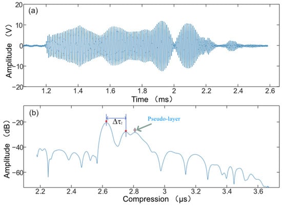
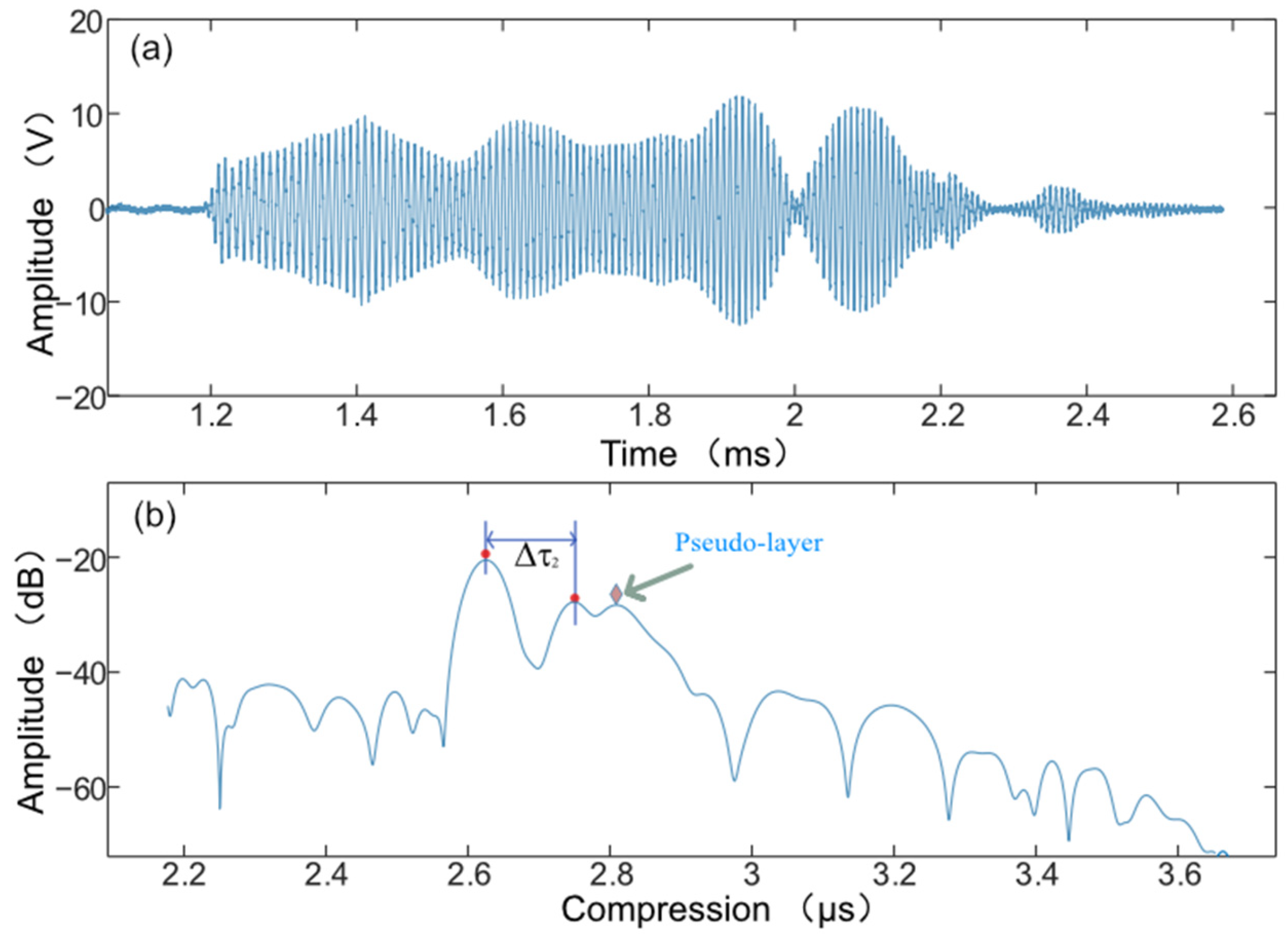
LFM measurements were subsequently performed on sediment Sample 3, with the received echo and corresponding pulse-compression result shown in Figure 10. As illustrated in Figure 10a,b, matched filtering of the raw waveform produces a pronounced double-peak feature to the right of the largest peak, making the pulse-compression result appear to indicate a three-layer structure. However, Sample 3 actually consists of only an upper mud layer overlying a sand layer, as marked in Figure 10b, indicating that the additional peak does not correspond to a real sediment interface. If the two left-hand peaks are nevertheless interpreted as the upper and lower interfaces, their inter-peak delay is Δt = 142 μs; using the measured mud-layer thickness D₀ = 91.0 mm then yields an apparent upper layer sound speed of c_{S_LFM} = 1281.69 m/s.

Figure 10. LFM pulse-compression measurement results for sediment Sample 3: (a) raw received echo; (b) pulse-compressed waveform.

4.3.2. Stepped-Frequency Interference and Sound-Speed Inversion

Stepped-frequency measurements were performed on Sample 3 over 95–125 kHz with a 1 kHz frequency increment; the measured echoes are shown in Figure 11a. Samples 2 and 3 were prepared simultaneously under the same conditions and therefore had similar upper layer sediment properties, differing primarily in layer thickness. Because the LFM-derived upper layer sound speed was below that of water, the upper layer acoustic impedance was inferred to be lower than the water impedance, corresponding to a negative reflection coefficient. A π phase reversal was therefore applied to the upper-interface echo in the simulations. Using the LFM-derived upper layer sound speed of 1281.69 m/s as the reference and keeping all other sonar parameters identical to those of the HF-SSBP, the simulated echoes shown in Figure 11b are obtained.

Figure 11. Measured and simulated stepped-frequency echoes for sediment Sample 3: (a) measured echoes; (b) simulated echoes using the LFM-derived sound speed as the reference.

Comparison of Figure 11a,b reveals a pronounced discrepancy in the amplitude evolution of the interference region. The simulation based on the LFM pulse-compression estimate of 1281.69 m/s therefore fails to reproduce the measured interference pattern, indicating a substantial bias in the LFM-derived sound speed.

4.3.3. Layer-Drift and Pseudo-Layer Diagnosis

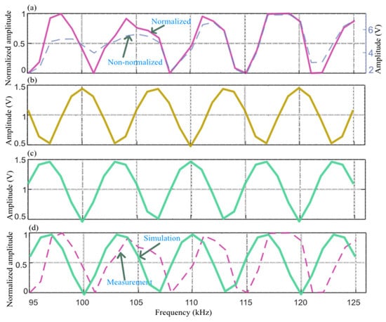
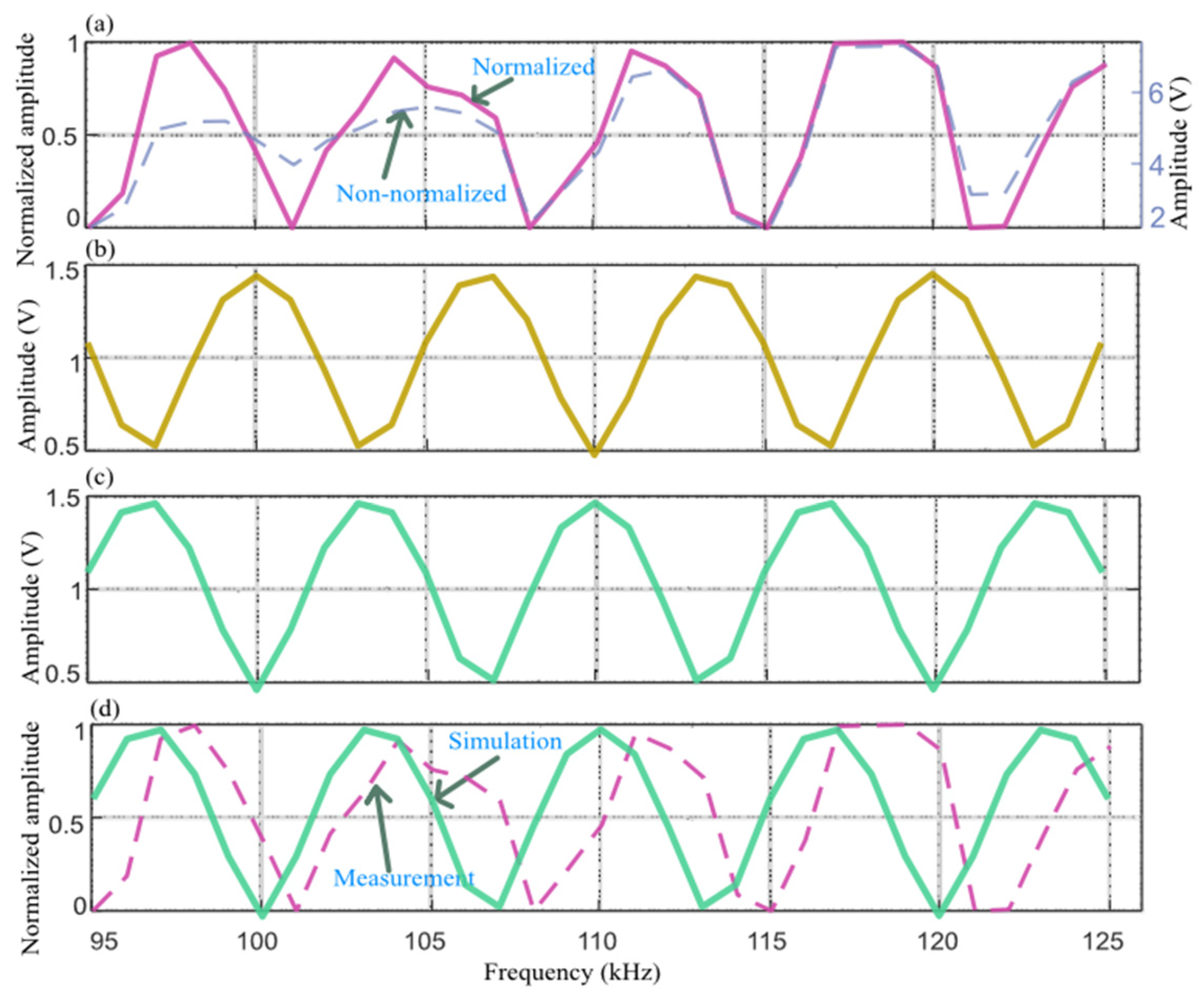
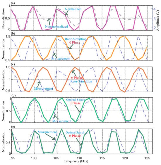
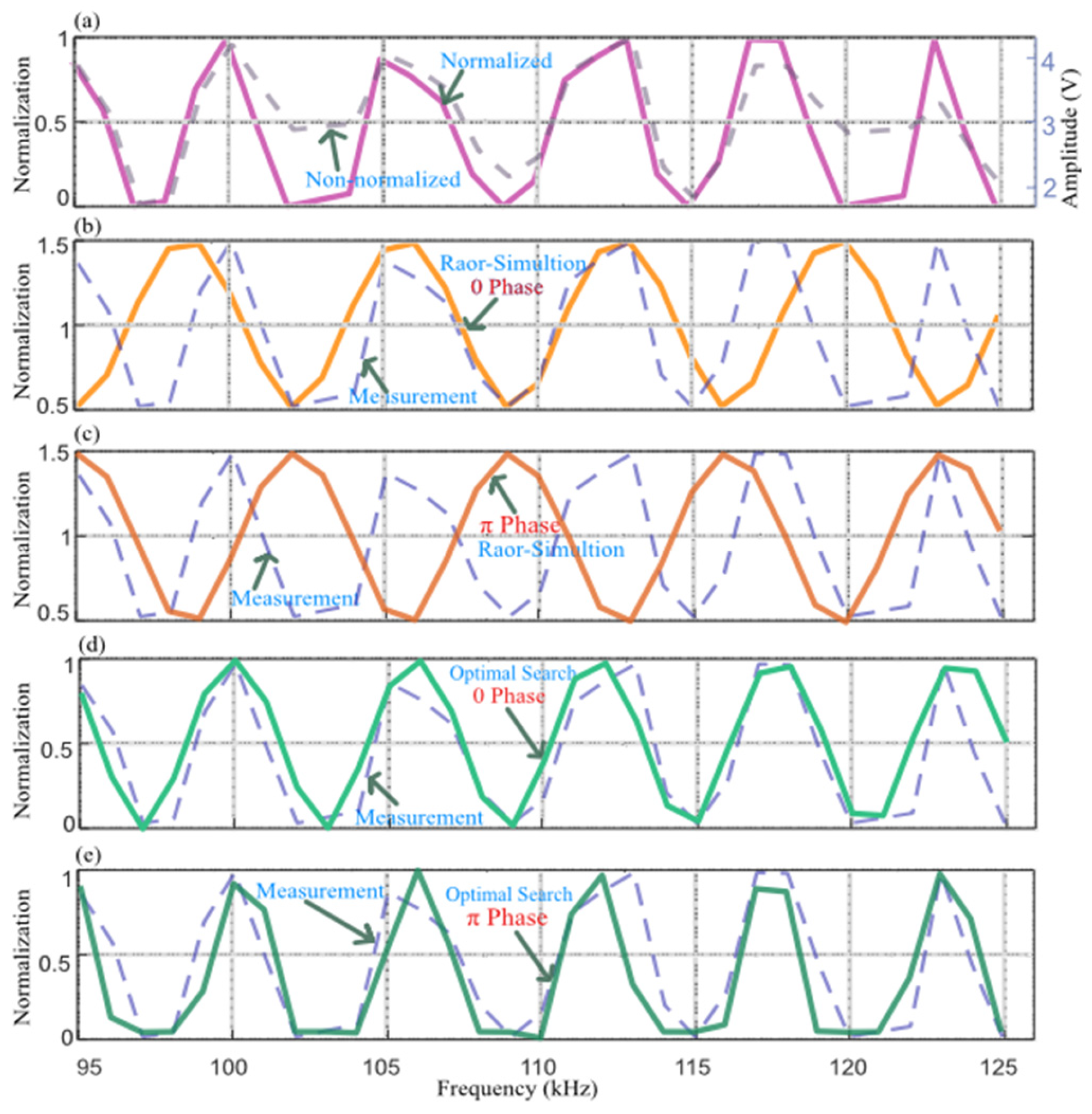
Figure 12a shows the interference-segment amplitudes extracted from the measured stepped-frequency echoes of Sample 3. The dashed curve is the unnormalized amplitude, and the solid curve is the segment-wise normalized amplitude. Figure 12b and Figure 12c show the interference amplitudes extracted from simulated stepped-frequency echoes using the LFM-derived sound speed of 1281.69 m/s as the reference, without and with a π phase reversal, respectively. Both simulated curves deviate substantially from the measurements, and the number of interference oscillation cycles is clearly different. The measured curve contains approximately 5.5 cycles, whereas the simulation based on the LFM sound speed contains only approximately 4.7 cycles. Thus, the LFM-referenced simulations cannot reproduce the observed interference response, demonstrating a marked error in the LFM-derived sound speed.

Figure 12. Interference-amplitude comparison and optimal sound-speed inversion for sediment Sample 3: (a) measured interference amplitude; (b) simulated interference amplitude without π phase reversal; (c) simulated interference amplitude with π phase reversal; (d) comparison between simulation and measurement at the 1070 m/s optimum; (e) comparison between simulation and measurement at the 1098 m/s optimum.

The optimal-sound-speed inversion procedure of Section 4.2.3 was therefore applied, using a search interval centered on the LFM estimate, [c_{S_LFM} − 400, c_{S_LFM} + 400] m/s, with a 1 m/s increment. At each candidate sound speed, the interference amplitude was simulated using the actual HF-SSBP parameters and compared with the measured interference amplitude using the Pearson correlation coefficient. The optimal sound speeds obtained without and with phase reversal were 1070 and 1098 m/s, respectively. Figure 12d,e compare the measured interference amplitude with simulations at these two optima. Relative to Figure 12b,c, the agreement between simulation and measurement is markedly improved. The Pearson correlation coefficient is 0.854 for Figure 12d at 1070 m/s and 0.876 for Figure 12e at 1098 m/s, with the latter providing the better match.

Figure 13 compares the simulated and measured waveforms of Sample 3 at all 31 frequencies for c_{S_SS} = 1098 m/s with the π phase reversal included. The two sets of waveforms show high similarity across the entire frequency set, indicating that the simulation under this condition reproduces the measured echoes well and confirming consistency between the adopted simulation parameters and the observations.

Figure 13. Waveform comparison between simulated and measured echoes for sediment Sample 3 at 31 frequencies for the 1098 m/s solution including the π phase reversal.

To independently validate the optimal sound speed of Sample 3, a 110 kHz burst signal consisting of 10 cosine cycles was also transmitted and the inter-interface delay was estimated using correlation. Because the mud layer in Sample 3 was relatively thick (91.0 mm), however, the mud–sand reflection was weak and its main lobe was strongly coupled to sidelobes of the upper-interface echo. A valid and stable correlation peak could not be obtained, and an independent burst-based sound speed was therefore unavailable. This failure is physically consistent with the layer-drift diagnosis described above: the weak lower-interface reflection and its susceptibility to distortion by upper-interface sidelobes are precisely the conditions that cause the LFM envelope peak to shift substantially. To compensate for the lack of an independent burst measurement, the point-by-point comparison in Figure 13 between simulated and measured echoes at all 31 frequencies under the 1098 m/s, π-reversal condition was used as evidence of internal consistency. The observed number of interference cycles (approximately 5.5 in the measurements compared with approximately 4.7 in the simulation referenced to the LFM sound speed) provides an additional independent constraint. It should nevertheless be noted that the optimal sound-speed estimate for Sample 3 is currently supported primarily by interference self-consistency and lacks conventional independent cross-validation. Future measurements should increase transmit power, extend the integration time, or improve the burst-mode signal-to-noise ratio to provide such validation.

Considering the simulation comparisons together with the facts that Samples 2 and 3 were prepared simultaneously under identical conditions, that the upper layer impedance is lower than that of water, and that a π phase reversal is therefore physically plausible, we conclude that the upper-interface echo of Sample 3 undergoes a π phase reversal and that the optimal upper layer sound speed is 1098 m/s. This value differs from the LFM-derived estimate of 1281.69 m/s by approximately 184 m/s, far exceeding the sound-speed deviation corresponding to a half-wavelength phase error (approximately 35 m/s). The LFM pulse-compression peak has therefore undergone substantial displacement, confirming pronounced layer drift in the LFM interpretation of Sample 3.

5. Discussion

5.1. LFM Layer Drift and Pseudo-Layer

According to Equation (4), the LFM pulse-compressed echo from a two-layer sediment can be regarded as the coherent superposition, in the time domain, of two Sa(·)-type components corresponding to the upper and lower layers. The resulting envelope depends not only on the amplitudes and time delays of the two echoes, but also on the phase difference between the two components, which is governed by the layer thickness. When the echo from the lower layer (or the upper layer) is relatively weak and its main lobe lies close in time to the sidelobe of the other layer echo, the sidelobe of the stronger echo can distort the main-lobe shape of the weaker echo. On the one hand, the compressed-peak position of the weak layer is shifted, producing layer drift; on the other hand, in-phase superposition of the two sidelobes can increase the sidelobe energy and generate a false local extremum, thereby forming a pseudo-layer.

The simulations in Section 4.1 (Figure 5) show that these two phenomena are not accidental, but depend on specific combinations of layer spacing, relative amplitude, and sound speed, and they often occur together. It should be emphasized that such deviations constitute a systematic coherent bias rather than random measurement noise. Importantly, whether a peak shift occurs is not determined simply by whether the layer spacing is smaller than the temporal resolution δ_t = 1/B = 33.3 μs. In the two samples investigated here, the echo-delay differences (approximately 142–150 μs) were both substantially larger than δ_t, and the two layers should therefore have been clearly resolvable according to the conventional resolution criterion; nevertheless, appreciable peak shifts could still occur. Consequently, errors arising from interpretation of the layer structure solely on the basis of LFM envelope peaks cannot, in principle, be eliminated merely by increasing the signal-to-noise ratio, and a phase-sensitive observable must be introduced for discrimination.

5.2. Discrimination of LFM Bias Using the Interference-Amplitude Method

Unlike LFM envelope detection, the frequency-swept amplitude method extracts, point by point along the frequency axis, the steady-state amplitude in the overlap region of the echoes from the first and lower layer. Because this observable is the steady-state amplitude resulting from the coherent superposition of two monochromatic signals, it does not involve the sidelobe coupling inherent in LFM pulse compression and is therefore, in principle, unaffected by the interference of layer drift and pseudo-layers with peak-position identification. This constitutes the physical basis of its discrimination capability.

It should be emphasized that whether peak displacement occurs is fundamentally determined by the relative amplitudes of the two components together with their relative phase Δφ (with an additional π phase reversal for a low-acoustic-impedance upper layer). When these quantities fall within an unfavorable coherent-superposition regime in which a sidelobe interferes adversely with a main lobe, the weak-layer peak can be displaced or even replaced by a pseudo-peak; otherwise, the correct peak position is retained. It is precisely this phase dependence that makes the LFM peak position highly sensitive to small perturbations in layer thickness and sound speed. The two samples investigated in this study show that a layer-thickness difference of only about 4.6 mm (86.4 mm versus 91.0 mm) can cause the LFM peak position to change abruptly from being essentially correct to exhibiting drift, because a change in D₀ simultaneously changes both the time delay Δt and the relative phase Δφ. Even a small perturbation may therefore move the observation condition from a favorable to an unfavorable interference regime, resulting in a step-like rather than gradual response to sound-speed perturbations. In contrast, the interference-amplitude method uses the oscillation period and peak–trough phase of the interference pattern as its observables; these quantities are independent of sidelobe coupling and can therefore provide a comparatively robust sound-speed inversion, while also enabling a more objective validation of the LFM peak interpretation.

5.3. Low-Impedance Criterion

Another key finding in the experiment is that, when the upper layer is highly porous fluid or soft mud containing microbubbles, its sound speed and acoustic impedance can be lower than those of water. The reflection coefficient at the water–sediment interface is then negative, causing the upper-interface echo to undergo a π phase reversal, whereas the phase of the mud–sand reflection remains unchanged. In the interference-amplitude-versus-frequency response, this behavior appears as a global interchange of peaks and troughs.

Mechanistically, introducing the π reversal is not a minor correction; it changes the sign of the interference term and therefore determines the direction of the optimum solution. If the effect is ignored, the peak–trough phase is shifted by half a cycle and the estimated sound speed acquires a directional systematic bias. Such a bias does not vanish through averaging or the addition of more data but remains consistently displaced to one side of the true solution. The π phase reversal must therefore be explicitly included in the interference model. Otherwise, an apparently good fit can represent a pseudo-solution generated by an incorrect physical model. Here, discrimination was achieved by comparing the agreement between measured interference amplitudes and models with and without π reversal. After the phase reversal was included, the simulated and measured peak–trough phases oscillated in the same direction, the correlation coefficient changed from negative to positive, and the optimal sound speed shifted toward the physically plausible range. Peak–trough inversion itself therefore provides direct evidence that the upper layer is a low-acoustic-impedance medium.

This criterion also has clear geological significance. Low-acoustic-impedance zones commonly correspond to highly porous, gas-bearing (microbubble-containing) fluid or soft muds whose acoustic properties contradict the conventional assumption that sediment impedance exceeds water impedance. Applying a conventional positive-polarity model to such materials can therefore introduce systematic interpretational errors. By identifying peak–trough inversion, the proposed interference-amplitude method not only improves the sound-speed estimate but also directly indicates whether the upper layer is a low-impedance medium, providing a new observational constraint for identifying and resolving ambiguities in fluid mud, unconsolidated soft mud, and related special sedimentary units.

5.4. Applicability and Limitations of the Method

The proposed method is intended primarily for measurements of shallow thin sediment layers. Its central purpose is to diagnose the layer structure inferred from LFM pulse compression (specifically, to identify layer drift and pseudo-layer) and then to refine the upper layer sound speed. Because the interference-amplitude method uses phase-sensitive information and is not affected by sidelobe coupling, its advantage is most pronounced when the LFM envelope approaches its resolution limit. It is particularly suited to thin bilayers consisting of surficial soft mud over sand, where the impedance contrast is strong and the upper layer impedance may fall below that of water. In such settings, conventional LFM envelope interpretation is prone to layer drift and pseudo-layer, whereas the interference method can still provide a reliable sound-speed estimate and identify the low-acoustic-impedance zone. The method therefore directly targets a regime in which LFM pulse compression is intrinsically vulnerable.

From an instrumentation perspective, the method benefits from the coherent reception and high amplitude/phase fidelity of the HF-SSBP and does not impose demanding data-acquisition or storage requirements. Nevertheless, stepped-frequency measurements are acquired sequentially, so the relative position of the transmitter–receiver platform must remain stable throughout the sweep. The approach is therefore most appropriate for fixed-station or low-speed survey operation; otherwise, platform displacement between frequency samples will distort the interference amplitude. This requirement differs from the single-pulse continuous-survey imaging mode of conventional LFM operation and constitutes an important practical boundary condition. The method also assumes that layer thickness is independently available. If thickness is completely unknown, both stepped-frequency interference and LFM travel-time measurements constrain only a thickness-to-sound-speed ratio, and one of the two variables must be supplied by prior information. In addition, the present model does not account for sediment attenuation, dispersion, or the frequency-dependent effective acoustic impedance of gas-bearing media. Dispersion may be non-negligible in microbubble-bearing low-impedance muds, and future work should therefore incorporate frequency-dependent attenuation and dispersion corrections.

6. Conclusions

This study addressed acoustic measurement of shallow low-acoustic-impedance two-layer sediments, typified by a soft-mud upper layer overlying sand. Using the self-developed HF-SSBP, we proposed a sound-speed inversion and layer-drift discrimination framework based on interference-phase self-consistency. The main conclusions are as follows:

(1)

LFM pulse compression can exhibit systematic errors in identifying thin two-layer structures because of coherent sidelobe superposition. These errors cannot be eliminated simply by increasing the signal-to-noise ratio. A layer-thickness difference of only approximately 4.6 mm caused the LFM peak interpretation to change from essentially correct to severely drifted, with the sound-speed discrepancy increasing from approximately 15 m/s to approximately 184 m/s. This result demonstrates that LFM-based layer identification can operate near a critical and inherently unstable regime. The proposed method effectively diagnoses the resulting layer drift and pseudo-layer.

(2)

The stepped-frequency interference-amplitude method is not affected by LFM sidelobe coupling and can accurately invert the upper layer sound speed when the layer thickness is independently known. For Sample 2, consistent results were obtained by the LFM, interference, and burst methods. Self-consistency between the interference-derived and LFM-derived sound speeds therefore provides an objective criterion for diagnosing layer drift.

(3)

When the upper layer acoustic impedance is lower than that of water, the reflected echo undergoes a π phase reversal that must be explicitly incorporated into the interference inversion. The resulting peak–trough inversion of the interference response itself provides a direct criterion for identifying a low-acoustic-impedance zone.

Overall, the proposed approach expands the measurement dimension from a single LFM waveform to a combined multifrequency observation and provides a new quantitative route for diagnosing LFM layer drift and inverting sound speed in thin low-acoustic-impedance sediments.

References

- Pan, F.; Wang, B.; Zhang, Y.; Zhang, X.; Cai, Y.; Liu, H.; Guo, Z.; Wang, X. Bioavailability, (im)mobilization kinetics, and spatiotemporal patterns of arsenic and cadmium in surficial sediments of a river–estuary–coast system. J. Hydrol. 2022, 612, 128140. [Google Scholar] [CrossRef] [Scilit]
- Zhao, B.; Wei, Q.; Han, Y.; Wang, X.; Zhang, Y.; Yi, M.; Wang, N.; Zhao, Z.; Wang, B.; Yao, P. Effects of oxygen penetration and iron redox shuttling on the preservation of reactive iron-bound organic carbon in a large-river-dominated estuary. Geochim. Cosmochim. Acta 2026, 417, 281–295. [Google Scholar] [CrossRef] [Scilit]
- Guilhermic, C.; Mouret, A.; Howa, H.; Metzger, E.; Couasnet, G.; Nardelli, M.P. Effects of frequent or massive sediment supplies on sediment redox dynamics: A microcosm simulation. Estuar. Coast. Shelf Sci. 2025, 324, 109472. [Google Scholar] [CrossRef] [Scilit]
- Kim, H.; Kawakatsu, H.; Akuhara, T.; Takeuchi, N. Characterizing the seafloor sediment layer using teleseismic body waves recorded by ocean bottom seismometers. J. Geophys. Res. Solid Earth 2023, 128, e2023JB027616. [Google Scholar] [CrossRef] [Scilit]
- Zhu, J.; Zhou, T.; Li, T.; Chen, B.; Meng, X.; Mazhar, S. High-resolution sub-bottom profiling technology using parametric array and vector hydrophone. Appl. Acoust. 2024, 223, 110077. [Google Scholar] [CrossRef] [Scilit]
- Zhang, X.; Yang, P.; Sun, M. Experiment results of a novel sub-bottom profiler using synthetic aperture technique. Curr. Sci. 2022, 122, 461–464. [Google Scholar] [CrossRef] [Scilit]
- Li, T.; Huang, Z.; Zhang, X.; Meng, F.; Pei, Y.; Guo, J. Application of pseudo-3D sub-bottom profile imaging technology in small submarine target detection. Acta Geophys. 2024, 73, 393–405. [Google Scholar] [CrossRef] [Scilit]
- Reis, G.C.; Santos, K.A.; Latrubesse, E.M.; Silva, G.M.; Zhou, F.; Formiga, K.T.M. Analysis of sub-bottom profile application to estimate sediment thickness over Itumbiara and Batalha HPP reservoirs, Brazil. CATENA 2025, 261, 109385. [Google Scholar] [CrossRef] [Scilit]
- Wang, L.; Li, J.; Zhao, J.; Bai, F.; Hu, B.; Dou, Y.; Song, W.; Zou, L. Sedimentation of tidal sand ridges off the Liuguhe River mouth in the Liaodong Bay, Bohai Sea. Mar. Geol. 2025, 480, 107473. [Google Scholar] [CrossRef] [Scilit]
- Hua, Q.; Wang, J.; Li, G.; Zhang, L.; Sun, L.; Dong, W. Time difference auto-extraction methods for in situ sound speed measurements in seafloor sediments. Geophys. Prospect. 2024, 72, 2261–2273. [Google Scholar] [CrossRef] [Scilit]
- Pfenninger, P.; Lin, Y.-T. Geoacoustic inversion of sub-bottom profile data using an autonomous underwater vehicle equipped with a sound source and towed hydrophone array. J. Acoust. Soc. Am. 2025, 158, 2602–2614. [Google Scholar] [CrossRef] [Scilit]
- Christopher, M.O.; DeCourcy, B.J.; Lavery, A.C.; Braun, C.D.; Bonnel, J. Low-frequency geoacoustic inversion of abyssal plain deep sediment properties near the Atlantis II Seamount. J. Acoust. Soc. Am. 2026, 160, 1147–1158. [Google Scholar] [CrossRef] [Scilit]
- Zhang, L.; Li, X.; Liu, L.; Meng, X.; Zhou, Q.; Liu, K.; Hua, Q.; Wang, J. Impedance inversion of high-frequency Chirp sub-bottom profiles constrained by borehole data. Mar. Georesour. Geotechnol. 2026, 44, 170–181. [Google Scholar] [CrossRef] [Scilit]
- Lima, A.L.M.; Neto, A.A.; Gallea, C.G.; de Freitas, B.L.; Clua, E.W.G.; Carvalho, L.F.R. Acoustic inversion of high-resolution seismic data applied to geotechnical characterization of marine sediments in the Campos Basin. Eng. Geol. 2026, 368, 108761. [Google Scholar] [CrossRef] [Scilit]
- Knobles, D.P.; Koch, R.A.; Thompson, L.A.; Focke, K.C.; Eisman, P.E. Broadband sound propagation in shallow water and geoacoustic inversion. J. Acoust. Soc. Am. 2003, 113, 205–222. [Google Scholar] [CrossRef] [Scilit]
- Knobles, D.P.; Wilson, P.S.; Goff, J.A.; Cho, S.E. Seabed acoustics of a sand ridge on the New Jersey continental shelf. J. Acoust. Soc. Am. 2008, 124, EL151–EL156. [Google Scholar] [CrossRef] [Scilit]
- Ma, Y.; Zhang, X.; Jiang, F.; Wei, Z.; Liu, C. Near-field geoacoustic inversion using bottom reflection signals via self-attention mechanism. IEEE J. Sel. Top. Appl. Earth Obs. Remote Sens. 2024, 17, 10545–10558. [Google Scholar] [CrossRef] [Scilit]
- Li, Z.; Zhang, J.; Yuan, Y.; Zhu, P.; Xu, Z.; Cai, W. Static-constrained first-arrival traveltime tomography for near-surface velocity estimation. Geophysics 2025, 90, U71–U82. [Google Scholar] [CrossRef] [Scilit]
- Fan, J.; Liu, X.; Yao, X.; Yang, Y. High-quality MIMO sonar imaging using cross correlation suppression. IEEE Geosci. Remote Sens. Lett. 2025, 22, 1–5. [Google Scholar] [CrossRef] [Scilit]
- Zhang, J.; Song, J.; Zhao, S. A high-resolution post-stack inversion method constrained by seismic waveform characteristics. IEEE Trans. Geosci. Remote Sens. 2025, 63, 1–10. [Google Scholar] [CrossRef] [Scilit]
- Dahlin, A.; Lecomte, I.; Senger, K.; Smyrak-Sikora, A.; Braathen, A.; Stemmerik, L. Analysing lithological complexity in outcrop-scale seismic models of interbedded siliciclastics and carbonates from Svalbard. Mar. Pet. Geol. 2025, 181, 107494. [Google Scholar] [CrossRef] [Scilit]
- Olsen, M.L.; Bredesen, K.; Nielsen, L.; Jusri, T.A.; Boldreel, L.O. Reliability of acoustic impedance inversion for seismic monitoring of gas in thin stacked reservoir zones: A case study from the Gassum Formation, Denmark. J. Appl. Geophy. 2026, 253, 106434. [Google Scholar] [CrossRef] [Scilit]
- Naseer, M.T. Spectral decomposition-based static reservoir simulations of gas-bearing cretaceous deep-water resources, SE-Indus delta. J. Appl. Geophy. 2025, 239, 105706. [Google Scholar] [CrossRef] [Scilit]
- Tian, Y.; Gao, J.; Wang, D.; Li, Z. Super-resolution optimal basic wavelet transform and its application in thin-bed thickness characterization. IEEE Trans. Geosci. Remote Sens. 2022, 60, 1–12. [Google Scholar] [CrossRef] [Scilit]
- Tian, Y.; Gao, J.; Chen, M.; Tao, C.; Meng, C. The fine characterization method of multiscale sedimentary cycles in phase space. IEEE Trans. Geosci. Remote Sens. 2025, 63, 1–13. [Google Scholar] [CrossRef] [Scilit]
- Lu, G.; Wang, C.; Zhang, X.; Lu, X.; Tang, R.; Zhang, S.; Wang, Z. High-resolution prediction of thin-layer reservoirs based on seismic sedimentology: A case study of the Penglaizhen Formation, Western Sichuan Basin, China. Nat. Resour. Res. 2025, 34, 2579–2598. [Google Scholar] [CrossRef] [Scilit]
- Katsman, R. Mechanics of methane bubbles in consolidated aquatic muds. Earth Sci. Rev. 2024, 257, 104908. [Google Scholar] [CrossRef] [Scilit]
- Katsnelson, B.; Uzhansky, E.; Lunkov, A.; Ostrovsky, I. Characterization of the gassy sediment layer in shallow water using an acoustical method: Lake Kinneret as a case study. Limnol. Oceanogr. Methods 2022, 20, 581–593. [Google Scholar] [CrossRef] [Scilit]
- Yi, B.-Y.; Kang, N.-K.; Hong, S.-H.; Kim, S.-R.; Choi, J.; Yoo, D.-G. Characterization of weak layers in the Southwestern slope of Ulleung Basin with seismic data merging and inversion. Mar. Geophys. Res. 2023, 44, 16. [Google Scholar] [CrossRef] [Scilit]
- Cao, X.; Qu, Z.; Shen, B.; Zhang, H. Illuminating centimeter-level resolution stratum via developed high-frequency sub-bottom profiler mounted on Deep-Sea Warrior deep-submergence vehicle. Mar. Georesour. Geotechnol. 2020, 39, 1296–1306. [Google Scholar] [CrossRef] [Scilit]
- Qu, Z.; Zou, D.; Shan, M.; Cao, X.; Xie, Y. Measuring the sound speed in deep-sea first sediment layer using a high-frequency submersible sub-bottom profiler: Method and sea trial application. Mar. Georesour. Geotechnol. 2022, 40, 1424–1434. [Google Scholar] [CrossRef] [Scilit]
- Zhen, H.; Cao, X.; Qu, Z.; Zou, D.; Xiong, S.; Song, J.; Guo, H. Sediment classification in the paleo-oceanic environment based on multi-acoustic reflectance characteristics in the Southern Tianshan Mountains. Front. Mar. Sci. 2024, 11, 1370274. [Google Scholar] [CrossRef] [Scilit]
- Qu, Z.; Shan, M.; Zou, D.; Cao, X.; Zhong, Z.; Xie, Y. Sampling guidance of deep-sea surficial sediment using acoustic faces CNN-BLSTM fusion. IEEE Geosci. Remote Sens. Lett. 2024, 21, 1–5. [Google Scholar] [CrossRef] [Scilit]
Disclaimer/Publisher’s Note: The statements, opinions and data contained in all publications are solely those of the individual author(s) and contributor(s) and not of MDPI and/or the editor(s). MDPI and/or the editor(s) disclaim responsibility for any injury to people or property resulting from any ideas, methods, instructions or products referred to in the content. |
© 2026 by the authors. Licensee MDPI, Basel, Switzerland. This article is an open access article distributed under the terms and conditions of the Creative Commons Attribution (CC BY) license.