


Abstract
Extracting instantaneous waterlines on tidal flats is challenging because spectral confusion among turbid water, wet bare tidal flats, and residual channel water can cause misclassification and boundary displacement. This study proposes a Topography-Guided Boundary U-Net (TGB-UNet) for Hangzhou Bay using Gaofen-1 and Gaofen-6 multispectral imagery. The model incorporates slope and local relative elevation through dual-scale topographic gating and topography-guided auxiliary boundary learning. Compared with FCN-8s, vanilla U-Net, and HED-UNet, TGB-UNet achieved the best mean performance across six evaluation metrics. Its F1 and boundary F1 scores reached 98.44% and 83.52%, respectively, while the average symmetric surface distance (ASSD) was 50.13 m, a reduction of 44.41% relative to vanilla U-Net. Ablation experiments showed that direct terrain concatenation did not yield consistent gains, whereas gated fusion and topography-guided boundary learning improved waterline localization. Tidal-level-stratified comparisons showed the largest absolute reductions in ASSD and the 90th-percentile boundary distance under low-tidal-level conditions. A spatial holdout test in an adjacent coastal sector further showed that TGB-UNet retained its advantage over vanilla U-Net across all six metrics. These results indicate that incorporating static topographic priors through dual-scale gating and topography-guided auxiliary boundary learning helps improve instantaneous waterline localization at complex water–land interfaces on tidal flats.
1. Introduction
Tidal flats occupy the dynamic interface between land and sea and provide important ecological and protective functions, including habitat provision, material cycling, and coastal protection, while being jointly influenced by tides, sediment transport, sea-level variations, and human activities [1]. Hangzhou Bay is a typical macrotidal and turbid bay, where broad and shallow tidal flats, tidal channels, islands and reefs, and artificial shorelines collectively form a complex water–land transition environment. In recent years, both the extent and morphology of the tidal flats in Hangzhou Bay have undergone pronounced changes [2]. Therefore, accurately delineating the instantaneous boundary between water and non-water at the time of image acquisition is essential for characterizing tidal-flat inundation and exposure patterns and for supporting coastal-zone management [3].
Early waterline extraction primarily relied on single-band thresholding, water indices, edge detection, and conventional classification methods; however, the performance of these methods was highly sensitive to tidal level, turbid water, wet bare tidal flats, and residual water in tidal channels, often necessitating scene-specific parameter tuning or manual correction [4,5,6,7]. In recent years, deep learning and multisource time-series imagery have substantially improved the automation of water-body extraction on tidal flats [8,9,10,11]. Semantic segmentation networks, such as fully convolutional networks (FCNs) and U-Net, can learn multiscale features and have been widely applied to water–land segmentation and coastline extraction [12,13,14,15,16,17,18]. However, these methods primarily optimize region-level overlap for water bodies, whereas waterline pixels account for only a small proportion of all pixels; consequently, high region-level F1-score or intersection-over-union (IoU) values do not necessarily guarantee continuous boundaries or accurate spatial localization [19].
To improve boundary quality, methods such as Gated-SCNN, HED-UNet, and SEANet have strengthened boundary learning through shape branches, edge detection, or multi-task supervision [20,21,22]. These approaches can reduce boundary smoothing and fragmentation; however, boundary discrimination still relies primarily on semantic, textural, and gradient cues derived from the imagery. When turbid water, wet bare tidal flats, and residual water in tidal channels exhibit similar spectral characteristics, these boundary-aware models may still misclassify pixels and displace the predicted water–land boundary. Terrain data can provide relatively stable spatial and geomorphological context; nevertheless, previous multimodal studies have shown that the benefit of auxiliary information depends strongly on the selected variables and fusion strategy [23,24,25,26,27,28]. Moreover, static terrain data cannot represent the actual tidal-flat elevation at the image acquisition time and are therefore unsuitable as a direct basis for water-body discrimination. Slope and local relative elevation characterize the local terrain gradient and the elevation of a pixel relative to its surroundings, respectively, providing auxiliary topographic context for discrimination based on optical imagery. Previous studies have incorporated slope and other terrain variables to support water-body extraction [25] and used topographic position indices based on elevation differences from the neighborhood mean to identify low-lying terrain and predict wetland distribution [29,30]. The contribution of auxiliary spatial variables depends on their physical meaning, spatial scale, integration strategy, and validation design. Geographic information system (GIS)-based multicriteria analysis provides a methodological context for combining spatial information [31], while research on spatial prediction emphasizes accounting for spatial dependence in predictor selection and validation to distinguish the reproduction of existing spatial patterns from transfer to unseen areas [32,33]. These studies inform the selection, integration, and spatial validation of auxiliary terrain information.
Previous studies have investigated water–land segmentation, boundary supervision, and terrain-information fusion. However, controlled comparisons have not sufficiently examined whether a static topographic prior can improve instantaneous waterline extraction or how terrain information should be integrated with optical features for segmentation and boundary discrimination. To address this gap, we use 44 Gaofen-1 (GF-1) and Gaofen-6 (GF-6) multispectral images of Hangzhou Bay and propose a Topography-Guided Boundary U-Net (TGB-UNet), in which slope and local relative elevation within a 330 m neighborhood (RE330) are employed as static topographic priors shared across acquisition dates. TGB-UNet selectively fuses terrain and optical features through dual-scale topographic gating and strengthens learning in water–land interface areas using a topography-guided auxiliary boundary head. The dataset was independently split by image acquisition date, and model performance was evaluated through model comparisons, ablation experiments, full-scene waterline evaluation, tidal-level-stratified analysis, and spatial generalization testing.
The remainder of this paper is organized as follows. Section 2 introduces the study area, data sources, and preprocessing procedures. Section 3 describes the architecture of TGB-UNet. Section 4 presents the experimental design and evaluation methods. Section 5 presents and discusses the experimental results, and Section 6 summarizes the main conclusions.
2. Study Area and Data
2.1. Study Area
Hangzhou Bay is located along the eastern coast of China, south of the Yangtze River Estuary, and constitutes an important estuarine bay connecting the Qiantang River Estuary with the East China Sea. The study area has a funnel-shaped morphology, with a wide bay mouth, a narrow upstream reach, shallow water depths, and strong tidal dynamics; these characteristics make Hangzhou Bay a typical macrotidal estuarine bay in China [34]. Under the combined influence of tidal dynamics, runoff from the Qiantang River, sediment transport, and human shoreline-development activities [35], extensive tidal flats have developed along the coast of Hangzhou Bay [36]. Moreover, the water–land transition zone contains spatially interspersed water bodies, exposed tidal flats, tidal channels, and artificial shorelines [37,38].
This study focused on the distribution of water and non-water areas across the tidal flats along the northern and southern shores of Hangzhou Bay. The data coverage of the main experiments is delineated by the red outline in the right-hand panel of Figure 1. Tidal-level variations, turbid water, and wet bare tidal flats contribute to weak spectral contrast and diffuse water–land boundaries in remote sensing imagery, posing challenges for water–land segmentation and instantaneous waterline localization. Accordingly, this study combined multitemporal GF multispectral imagery with terrain information derived from Copernicus GLO-30 to evaluate the contributions of topographic gating and topography-guided auxiliary boundary learning to water–land segmentation and instantaneous waterline extraction on tidal flats. In addition, an adjacent coastal sector southeast of the main experimental area was designated for spatial generalization testing, with its data coverage delineated by the green outline in the right-hand map of Figure 1. This coastal sector was not used for model training or validation and provided a supplementary assessment of spatial transfer performance in an unseen coastal sector.
Figure 1.
Location of the study area and spatial coverage of the experimental data. The (left)-hand map shows the location of Hangzhou Bay within China. In the (right)-hand map, the red and green outlines indicate the spatial coverage of the main experimental data and the data used for spatial generalization testing in an additional coastal sector, respectively.
2.2. Data Sources
2.2.1. Gaofen-Series Multispectral Imagery
Wide-field-of-view (WFV) multispectral imagery from Gaofen-1 (GF-1) and Gaofen-6 (GF-6), both with a nominal revisit period of approximately 4 days, was selected as the primary optical remote sensing data source. The data were obtained from the National Remote Sensing Data and Application Service Platform at https://www.cpeos.org.cn (accessed on 5 July 2026). Image selection was based primarily on complete coverage of the study area and low cloud cover. Images with cloud cover below 10% and without extensive cloud obstruction over the study area were selected, with preference given to images exhibiting minimal cloud and haze obstruction and relatively clear textures in the shoreline and tidal-flat areas. All Gaofen data were obtained as Level-1A products with a spatial resolution of 16 m. To ensure a consistent four-band input configuration for images from the two satellites, the spectral bands shared by GF-1 and GF-6—blue, green, red, and near-infrared (NIR)—were used for model training, whereas the additional red-edge, violet, and yellow bands of GF-6 were excluded from the model inputs [39,40].
2.2.2. Copernicus DEM GLO-30
To incorporate topographic background information beyond optical imagery, Copernicus DEM GLO-30 was selected as the baseline elevation dataset. The product was primarily generated from observations acquired by the TanDEM-X mission between 2011 and 2015 and provides globally continuous surface elevation information at a spatial resolution of approximately 30 m. Unlike a bare-earth digital elevation model (DEM), GLO-30 is a digital surface model (DSM), and its elevation values may be influenced by vegetation, artificial structures, and the treatment of water bodies [41]. Therefore, this study used only the coarse-scale elevation differences and spatial terrain patterns represented by GLO-30. The dataset was treated as a relatively stable topographic prior rather than as a precise, contemporaneous observation of tidal-flat topography at the GF image acquisition dates. The data covering the study area were obtained from the public Copernicus DEM data source, with World Geodetic System 1984 (WGS 84) used as the horizontal datum and Earth Gravitational Model 2008 (EGM2008) as the vertical datum [42,43].
2.2.3. Tidal-Level Data
To analyze the influence of tidal-level variations on waterline extraction, hourly tidal-level data from the Zhapu tidal gauge station were obtained from the National Marine Science Data Center. According to the acquisition time of each GF image, the corresponding tidal level at the image acquisition time was matched, and the test images were subsequently divided into high-, intermediate-, and low-tidal-level groups. The tidal-level data were used solely to analyze model performance across tidal-level groups and were not involved in model training.
2.3. Data Preprocessing
To construct a multisource dataset with strict pixel-level correspondence among optical imagery, terrain variables, and water-body labels, GF image preprocessing, terrain feature construction, and synchronized patch extraction were performed. All data were transformed to the WGS 84/UTM Zone 51N projected coordinate system (EPSG:32651), and the geometrically corrected GF imagery was used as the spatial reference, with all datasets standardized to a spatial resolution of 15 m. Terrain variables and labels were co-registered according to the spatial extent, grid origin, and pixel size of the GF imagery, ensuring identical numbers of rows and columns and consistent pixel locations across all data sources. Continuous optical and terrain variables were resampled using bilinear interpolation, whereas binary labels were resampled using the nearest-neighbor method to avoid introducing new label classes. Pixels outside the study area or lacking valid reference labels were assigned a value of 255 and were excluded from model training and performance evaluation.
2.3.1. GF Image Preprocessing
GF-1 and GF-6 Level-1A multispectral images were sequentially subjected to radiometric calibration, atmospheric correction, and orthorectification to reduce the influence of differences in sensor response, atmospheric conditions, and imaging geometry on image spectra and spatial positioning. Subsequently, the four spectral bands shared by GF-1 and GF-6—blue, green, red, and near-infrared (NIR)—were selected, and the images were cropped and spatially aligned according to the study-area extent to generate full-scene GF images with consistent band composition, projected coordinate system, and pixel grid. The additional red-edge, violet, and yellow bands of GF-6 were excluded from model training to maintain the same four-band input configuration for both satellite sensors.
2.3.2. Terrain Feature Construction and Spatial Alignment
Copernicus DEM GLO-30 was first transformed to the projected coordinate system of the study area, and outliers and invalid values were subsequently processed. Slope and local relative elevation within a 330 m neighborhood were then calculated from the original 30 m terrain grid. The local relative elevation was denoted as RE330 and was defined as the difference between the elevation of the center pixel and the mean elevation of valid pixels within its 11 × 11 pixel neighborhood:
In the equation, denotes the elevation of the center pixel, denotes the 11 × 11 pixel neighborhood centered on that pixel, and denotes the number of valid pixels within . Because the spatial resolution of GLO-30 was 30 m, this neighborhood corresponded to a spatial extent of approximately 330 m × 330 m. A positive RE330 value indicated that the center pixel was higher than the local mean terrain elevation, whereas a negative RE330 value indicated that it was lower than the local mean terrain elevation. Invalid pixels were excluded from the neighborhood averaging. After RE330 was calculated on the original terrain grid, it was resampled to 15 m and spatially co-registered with the GF imagery.
2.3.3. Sample Patch Extraction and Label Generation
Because existing public datasets could not provide water-body labels and instantaneous waterline reference data that matched the GF imagery used in this study in terms of acquisition time, spatial extent, and spatial resolution, reference labels were constructed by combining machine-assisted interpretation with manual revision, and waterline vectors were generated simultaneously. The preprocessed GF-1 and GF-6 multispectral imagery was used as the primary basis for interpretation. Subsequently, the imagery was cropped into 512 × 512 image patches using a sliding-window approach with a stride of 256 pixels, and a total of 3099 samples containing both water and land areas were selected within the main experimental area.
Initial water-body masks were generated using the Segment Anything Model [44,45]. The resulting water-body boundaries were then inspected and corrected pixel by pixel with reference to GF multispectral composite imagery [46]. The main water bodies and tidal flats inundated at the image acquisition time were labeled as water, whereas exposed tidal flats, vegetation, artificial structures, and other land areas were labeled as non-water. Areas with ambiguous boundaries, shadow interference, or a high proportion of mixed pixels were repeatedly inspected. Manual annotation followed a two-person workflow in which one annotator performed the initial delineation and a second reviewed and corrected it to identify and rectify evident interpretation errors in the reference waterlines. Finally, label values of 1, 0, and 255 were assigned to water, non-water, and invalid regions, respectively.
After the image patches were annotated, the labels were reconstructed over the entire main experimental area for each acquisition date, and the patch boundaries and overlapping regions were subsequently inspected. The boundary between water and non-water areas was then extracted from the full-scene reference labels for each date, yielding instantaneous waterline reference data for 44 acquisition dates. Finally, the dataset was split by acquisition date [33], with 26, 9, and 9 complete acquisition dates assigned to the training, validation, and test sets, respectively. Data from the coastal sector designated for spatial generalization testing, outlined in green in the right-hand map of Figure 1, were separate from the main experimental dataset and were not included in model training or validation. The detailed test configuration is described in Section 4.5.
3. Methodology
3.1. Workflow
To address the pronounced spectral confusion between water bodies and wet bare tidal flats in Hangzhou Bay, as well as the ambiguous boundaries in water–land transition areas, this study focused on multisource data construction, topography-guided water–land segmentation, full-scene waterline extraction, and performance evaluation. The overall technical workflow is illustrated in Figure 2. Specifically, the research workflow comprised three main stages: multisource data preprocessing and training-sample construction; training and experimental design of the topography-guided water–land segmentation model; and full-scene reconstruction, waterline extraction, and performance evaluation for each acquisition date.
Figure 2.
Technical workflow of the proposed method.
3.2. TGB-UNet Architecture
The contracting–expanding architecture of U-Net enables the recovery of pixel-level spatial details while extracting contextual information and has become one of the commonly used approaches for sea–land segmentation. However, in the tidal-flat areas of Hangzhou Bay, strong spectral confusion exists among water bodies, wet bare tidal flats, and turbid water. Consequently, relying solely on GF imagery can lead to local misclassification and boundary displacement, resulting in inaccurate segmentation predictions and poorly defined boundaries.
On the other hand, standalone edge-detection methods can enhance gradient and contour information in imagery; however, edges themselves do not convey the class semantics of water and non-water and are therefore susceptible to interference from non-target linear features such as tidal channels, aquaculture ponds, roads, and tidal-flat surface textures. Consequently, relying solely on edge detection makes it difficult to determine the land-cover classes on both sides of an edge and to directly derive a continuous tidal-flat waterline with explicit geographic meaning.
To address the aforementioned issues, an improved U-Net model that jointly accounted for water-body region segmentation and water–land boundary learning was developed, as illustrated in Figure 3. GF multispectral imagery served as the primary information source, while slope and local relative elevation served as auxiliary topographic priors. Dual-scale topographic gating used these priors to modulate optical features at the shallow and intermediate encoder stages. A topography-guided auxiliary boundary head was then added to strengthen feature learning at water–land interfaces, while water–land segmentation remained the primary task. Patch-level water-body probability maps were first generated and then mosaicked into a full-scene water–land segmentation map for each acquisition date using coordinate-based spatial weighting. The waterline was then extracted and vectorized from the full-scene water-body extent. Overall, region-level semantics, topographic priors, and boundary constraints were integrated to establish a complete workflow from water–land segmentation to geospatial waterline extraction.
Figure 3.
Architecture of the proposed TGB-UNet. Blue represents encoder and decoder feature maps, and red represents bottleneck feature maps. Yellow represents the topographic gating modules G1 and G2 at the first and second encoder stages, respectively. Green represents water–land segmentation, and purple represents topography-guided auxiliary boundary learning.
3.3. Dual-Scale Topographic Gating
Water–land boundaries on tidal flats are primarily identified from optical imagery based on spectral differences, although their spatial distribution is also influenced by local terrain conditions. Slope characterizes local relief of the tidal-flat surface, whereas RE330 reflects the elevation relationship of a pixel relative to its local background and can therefore provide supplementary information for discriminating spectrally confused areas such as wet bare tidal flats, shallow-water areas, and tidal channels. Previous studies have shown that terrain information can support shoreline identification when digital elevation models (DEMs) and remote sensing imagery are jointly incorporated into segmentation networks [47]. However, static terrain does not directly represent water-body distribution at the image acquisition time, and its spatial resolution and error characteristics differ from those of optical imagery. Direct channel concatenation may not adequately control the relative contributions of spectral and terrain inputs, allowing terrain errors or spatial mismatches to propagate into the backbone network.
Gated fusion was adopted as a more appropriate strategy for controlling the contribution of auxiliary information [48,49]. Considering the limited number of terrain variables used in this study and their intended role in assisting optical feature discrimination, an independent deep terrain encoder was not constructed. Instead, lightweight topographic gating modules were incorporated into the first two encoder stages of U-Net [50,51], corresponding to G1 and G2 in Figure 3.
Slope and local relative elevation within a 330 m neighborhood were used to construct the terrain input. At the first scale, topographic gating was applied to high-resolution shallow features, where local slope variations and relative elevation differences were primarily used to supplement boundary details. At the second scale, the terrain input was downsampled by a factor of 2 using average pooling and was then used to generate a gating map for the intermediate encoder features; the pooling operation reduced local variation and provided a more spatially continuous representation of the topographic background. For each scale, the terrain features were transformed through convolutional mapping, and a bounded modulation map was generated using the hyperbolic tangent function (tanh):
Subsequently, residual gating was applied to modulate the optical features:
where represented the learnable gating strength constrained by the sigmoid function. This formulation allowed terrain information to enhance or suppress optical responses in a spatially adaptive manner while preserving the original optical feature pathway, thereby preventing low-quality or mismatched terrain information from exerting a dominant influence on the segmentation results.
After conditional topographic modulation at the first two encoder stages, the gated optical features were propagated through the remaining encoder stages. The modulated features also entered the decoder through skip connections, allowing the topographic priors to influence the main segmentation representation.
3.4. Topography-Guided Auxiliary Boundary Head
Although successive downsampling in U-Net expands the receptive field and facilitates the extraction of high-level semantic features, it can also remove spatial detail, leading to boundary displacement or excessive smoothing at water–land interfaces [52,53]. To alleviate the insufficient constraint imposed on boundary pixels by region segmentation loss, previous studies have introduced independent shape branches or auxiliary supervision for semantic boundaries. Ishikawa and Aoki [54] incorporated semantic boundary detection as an auxiliary task to improve boundary feature learning in the segmentation backbone. For remote sensing imagery, BGSC-Net further fused multiscale decoder features and applied explicit boundary supervision [55]. Collectively, these studies indicate that introducing a dedicated learning task for sparse boundary pixels can compensate for the weak boundary supervision provided by region-level segmentation losses [56].
Conventional auxiliary boundary heads typically predict boundaries directly from decoder features. However, in tidal-flat imagery, wet bare tidal flats, turbid water, and residual water in tidal channels exhibit similar spectral responses, and relying solely on decoder semantics or local textures can easily produce spurious boundaries. Therefore, a topography-guided auxiliary boundary head was incorporated after the final decoder features, allowing slope and RE330 to participate directly in boundary discrimination. This module consisted of three components: terrain feature mapping, decoder–terrain feature fusion, and boundary prediction.
The module simultaneously received the features output by the final decoder stage of U-Net and the terrain features spatially aligned with the imagery. The terrain input was transformed into 16-channel terrain features using a 3 × 3 convolution, followed sequentially by batch normalization (BN) and rectified linear unit (ReLU) activation:
Subsequently, was concatenated with the decoder feature along the channel dimension to obtain the joint feature representation . The boundary prediction head then fused spectral semantics and terrain information using a 3 × 3 convolution, followed by a 1 × 1 convolution to output a single-channel boundary response:
where represents the boundary probability map. Only a small number of convolutional operations were added at the final decoder stage, and therefore the network complexity was not substantially increased. Compared with a conventional auxiliary boundary head that relied solely on the decoder feature , the proposed structure allowed boundary prediction to depend jointly on water–land semantic information and local terrain conditions, thereby helping to suppress spurious boundaries caused by tidal-flat surface textures, turbid water, and residual water in tidal channels.
During training, the topography-guided auxiliary boundary head was supervised using single-pixel-wide inner water-boundary labels, and its gradients contributed to the optimization of the main network through the shared decoder features. This branch enhanced the network’s boundary representation and produced a boundary-probability map, whereas the final water–land segmentation map was generated by the main segmentation head.
3.5. Loss Function
For water–land segmentation on tidal flats, both the integrity of water-body regions and accurate localization of the water–land interface were required. Because interior pixels greatly outnumbered boundary pixels, a conventional region-level segmentation loss was dominated by large homogeneous regions and provided relatively weak supervision for the sparse boundary pixels. Therefore, a main segmentation loss and an auxiliary boundary loss were separately defined in this study.
The main segmentation task employed Dice loss and binary cross-entropy (BCE) loss [57]. Dice loss was used to maximize overlap between the predicted and reference water-body masks and to reduce the influence of class imbalance, whereas BCE loss provided pixel-wise probabilistic supervision for water/non-water classification [58,59]. The main segmentation loss was defined as follows:
The auxiliary boundary task employed class-balanced BCE loss and boundary Dice loss. The class-balanced BCE loss separately computed the mean errors over boundary and non-boundary pixels, thereby preventing the substantially larger number of non-boundary pixels from dominating the training process. In addition, boundary Dice loss was used to improve the overlap between the predicted and ground-truth boundaries. The auxiliary boundary loss was defined as follows:
The total loss was composed of the main segmentation loss and the auxiliary boundary loss:
where , the auxiliary boundary loss weight, was set to 0.1. This weighting ensured that the main segmentation task remained dominant during training while boundary supervision was used to improve the response of the shared features to the water–land interface. Invalid regions with a label value of 255 were excluded from the loss calculation.
4. Experimental Setup and Evaluation
4.1. Experimental Environment
All experiments were conducted on a Windows 10 workstation equipped with an NVIDIA GeForce RTX 3090 graphics processing unit (GPU; NVIDIA Corporation, Santa Clara, CA, USA). The models were implemented in Python 3.8.20 using PyTorch 2.4.1, with CUDA 11.8 and cuDNN 9.1.0 providing GPU acceleration. All models were trained for 150 epochs with a batch size of 8 using the AdamW optimizer [60]; the initial learning rate and weight-decay coefficient were both set to 1 × 10⁻⁴. During training, a cosine annealing schedule [61] was adopted to progressively reduce the learning rate.
Because M0 was identical to vanilla U-Net and M5 was identical to TGB-UNet, the same trained checkpoints and test results were reused in the model-comparison and ablation analyses. The same dataset split and training parameters were used for all runs, and the best-performing model weights were selected based on validation-set performance and subsequently evaluated on the test set. Finally, the results were reported as the mean ± standard deviation over the three independent runs.
4.2. Experimental Setup for Model Comparisons
To evaluate the effectiveness of the proposed method for water–land segmentation and instantaneous waterline extraction on tidal flats, three representative semantic segmentation networks—FCN-8s, vanilla U-Net, and HED-UNet—were selected for comparison. These three models used four-band GF imagery as input, whereas TGB-UNet additionally incorporated slope and RE330. All models followed the same dataset split, training strategy, and model selection criteria. Model performance was evaluated in terms of patch-level water-body segmentation and full-scene waterline localization, using the metrics described in Section 4.6.
FCN-8s: VGG16 was used as the encoder, and spatial resolution was progressively restored through feature fusion across different hierarchical levels followed by transposed convolution. This model was used to evaluate the performance of a representative fully convolutional semantic segmentation method for water-body extraction on tidal flats.
Vanilla U-Net: A symmetric encoder–decoder architecture was adopted, with shallow spatial information propagated through skip connections. Vanilla U-Net served as both the backbone of the proposed model and the primary comparison baseline.
HED-UNet: Based on the shared features, region segmentation and edge detection were jointly performed, and multiscale edge supervision was used to improve water–land boundary extraction. This model served as a boundary-aware baseline combining region segmentation and edge detection, enabling evaluation of the proposed method against an existing boundary-aware network.
TGB-UNet: The proposed model added dual-scale topographic gating and a topography-guided auxiliary boundary head to U-Net. Four-band GF imagery, slope, and RE330 were used as inputs, and the gating modules adaptively fused topographic information with optical features. The auxiliary boundary branch further used topographic features to strengthen representation learning at the water–land interface.
4.3. Ablation Study Design
To evaluate the effects of terrain-fusion schemes and auxiliary boundary learning on model performance, six ablation configurations (M0–M5) were designed. M0 used vanilla U-Net with only four-band GF imagery as input and served as the baseline. M1 concatenated slope and RE330 with the four GF bands at the input level, forming a six-channel input, to examine whether direct terrain concatenation improved performance. M2 replaced input-level concatenation with dual-scale topographic gating: the four-band GF imagery entered the main encoder, while slope and RE330 modulated optical features at the first two encoder stages through gating. This configuration enabled a comparison between the two terrain-fusion schemes. M3 added a conventional auxiliary boundary head to M2. This head received only the final decoder features and was used to evaluate the contribution of auxiliary boundary supervision. M4 incorporated a topography-guided auxiliary boundary head into vanilla U-Net, jointly using decoder and terrain features for boundary prediction without topographic gating in the encoder. M5 was the complete TGB-UNet, combining dual-scale topographic gating with the topography-guided auxiliary boundary head. Comparing M3 with M5 evaluated the contribution of the topography-guided auxiliary boundary head relative to the conventional auxiliary boundary head. Comparing M4 with M5 assessed the additional contribution of encoder-stage topographic gating when topography-guided boundary learning was already present. All configurations used the same dataset split, training settings, and model selection criteria.
4.4. Tidal-Level Grouping and Stratified Evaluation
According to the image acquisition times recorded in the GF image metadata, the nine test images were matched with hourly tidal-level data from the Zhapu tidal gauge station to obtain the tidal level corresponding to each image acquisition time. For images acquired at non-hourly times, the tidal level was interpolated from the values at the two adjacent full hours. Considering the limited number of images in the test set, the nine images were ranked from low to high tidal level and sequentially divided into low-, intermediate-, and high-tidal-level groups, with three images assigned to each group to ensure an equal number of samples among the groups. On this basis, the evaluation metrics of vanilla U-Net and the proposed model were separately calculated for the different tidal-level groups to analyze variations in model performance under different tidal-level conditions. The tidal levels and tidal phases corresponding to the test images are presented in Table 1.
Table 1.
Tidal-level grouping of the test dataset.
4.5. Spatial Generalization Test Setup
To evaluate model performance in a coastal sector not used for training or validation, spatial generalization testing was conducted in the area outlined in green in the right-hand map of Figure 1. This coastal sector is located southeast of the main experimental area, with no spatial overlap between their image-patch footprints. The test used GF imagery from six acquisition dates included in the main experimental test set, with twelve 512 × 512-pixel patches per date, yielding 72 samples in total.
Vanilla U-Net and TGB-UNet were compared using the best-performing model weights selected in the main experiments for each of the three random seeds. Inference was performed directly, without additional training or fine-tuning. The input configurations, preprocessing, and prediction postprocessing procedures were consistent with those used in the main experiments. Both models were evaluated over the same valid spatial extent using the metrics described in Section 4.6, and the results were reported as the mean and standard deviation across the three random seeds.
4.6. Evaluation Metrics
Model performance was evaluated at two levels: patch-level water-body segmentation and full-scene waterline localization [62,63]. Water–land segmentation metrics were calculated at the scale of 512 × 512 image patches to quantify the accuracy of water-body region identification. In contrast, waterline metrics were calculated after the probability image patches from the same acquisition date were mosaicked using spatial weighting, thereby evaluating boundary matching and distance errors at the full-scene scale.
For all evaluation metrics, the water class was treated as the positive class, with water labeled as 1 and non-water as 0. The predicted water-body probability maps were binarized using a fixed threshold of 0.5. The validation set was used solely for model selection, whereas the final performance metrics were calculated on the independent test set.
4.6.1. Segmentation Metrics
Water–land segmentation performance was evaluated using intersection over union (IoU) and the F1-score. Here, true positives (TP), false positives (FP), and false negatives (FN) were defined as correctly identified water pixels, non-water pixels incorrectly classified as water, and water pixels that were not identified, respectively. The metrics were calculated as follows:
IoU quantified the degree of overlap between the predicted and reference water-body regions, whereas the F1 jointly accounted for false positives and false negatives. These metrics were first calculated independently for each image patch and were then arithmetically averaged over all valid image patches in the test set.
4.6.2. Waterline Evaluation Metrics
Waterline boundary agreement was evaluated using the boundary F1-score (BF1) [64]. Considering that raster labeling, image co-registration, and boundary extraction could introduce small pixel-level deviations, a matching tolerance of 3 pixels was adopted for the calculation. Boundary precision was defined as the proportion of predicted boundary pixels that matched the reference boundary, whereas boundary recall was defined as the proportion of reference boundary pixels covered by the predicted boundary. A BF1 value closer to 100% indicated a higher degree of agreement between the predicted waterline and the reference waterline within the specified tolerance. BF1 was defined as follows:
Waterline positional errors were calculated from the bidirectional nearest-neighbor distances between the predicted and reference boundaries, with distances expressed in meters [65]. The average symmetric surface distance (ASSD) and the 90th-percentile distance (P90) were adopted for evaluation. ASSD was calculated as the mean bidirectional distance between the predicted waterline and the reference waterline and was used to characterize the overall mean positional deviation of the waterline [63,66]. P90 represented the distance below which 90% of the bidirectional boundary distances fell, thereby characterizing the control of relatively large positional deviations along the waterline. Lower ASSD and P90 values indicated greater spatial agreement between the predicted waterline and the reference waterline. Furthermore, the waterline length relative error (WLRE) was introduced to evaluate the difference in total length between the predicted and reference waterlines. Within the same valid evaluation extent, the total lengths of the predicted and reference waterlines were calculated separately, and WLRE was defined as follows:
where and denote the total lengths of the predicted and reference waterlines, respectively. A lower WLRE value indicated a smaller difference in total length between the two waterlines.
5. Results and Discussion
5.1. Performance Comparison of Different Models
Table 2 presents the water-body segmentation and waterline extraction results of the models on the test set. All values are reported as the mean ± standard deviation of results obtained from three independent training runs with different random seeds. TGB-UNet achieved the best mean performance across all six metrics, with F1, IoU, and BF1 values of 98.44%, 97.17%, and 83.52%, respectively, and ASSD, P90, and WLRE values of 50.13 m, 85.67 m, and 5.56%, respectively. Compared with the primary baseline, vanilla U-Net, TGB-UNet improved F1, IoU, and BF1 by 3.03, 2.49, and 3.13 percentage points, respectively, while reducing ASSD, P90, and WLRE by 44.41%, 32.16%, and 28.35%, respectively. These improvements covered both water-body region identification and waterline spatial localization.
Table 2.
Water–land segmentation and waterline extraction results of different models. Bold values indicate the best performance for each metric.
FCN-8s and vanilla U-Net exhibited similar region-level segmentation performance. Although vanilla U-Net achieved a higher BF1 and a lower ASSD, its P90 did not improve correspondingly. In contrast, HED-UNet, which jointly performs region segmentation and edge detection, further reduced ASSD to 55.19 m and P90 to 100.16 m, indicating that boundary learning helps alleviate localization errors associated with relying solely on region segmentation. Compared with HED-UNet, TGB-UNet further reduced ASSD and P90 by 5.06 m and 14.49 m, respectively, improving waterline-localization accuracy beyond that achieved by the existing boundary-aware model.
Full-scene waterline evaluation results for the individual test dates are provided in Table S1 of the Supplementary Materials. TGB-UNet achieved lower mean ASSD and P90 values than both Vanilla U-Net and HED-UNet on all nine dates, while its mean BF1 was higher than those of Vanilla U-Net and HED-UNet on nine and seven dates, respectively. To further examine the consistency of these improvements across the test dates, the nine dates were treated as paired statistical units. Two-sided Wilcoxon signed-rank tests were used to evaluate the differences between TGB-UNet and the baseline models, and the resulting p-values were adjusted for multiple comparisons using the Holm method. The 95% confidence intervals of the mean improvements were estimated by date-level bootstrapping, and the complete results are reported in Table S2 of the Supplementary Materials. After adjustment, the improvements of TGB-UNet over Vanilla U-Net were statistically significant for BF1, ASSD, and P90. Compared with HED-UNet, the improvements in ASSD and P90 were statistically significant, whereas the difference in BF1 did not reach statistical significance. These results indicate that the improvements in waterline localization over Vanilla U-Net were reasonably consistent across the test dates and were not driven primarily by large gains on only a few dates. Compared with the boundary-aware HED-UNet, the advantage of TGB-UNet was expressed mainly as reductions in the mean positional error and relatively large positional deviations, whereas the additional improvement in boundary matching within the three-pixel tolerance was comparatively limited. This finding further suggests that the principal benefit of topographic guidance lies in reducing the spatial positional errors of the extracted waterlines rather than merely increasing the number of boundary matches within the specified tolerance.
To examine the sensitivity of boundary-matching results to the tolerance setting, BF1 was further compared across models at tolerances of 1–5 pixels. As shown in Figure 4, BF1 increased progressively for all models as the matching tolerance increased. TGB-UNet consistently achieved the highest mean BF1, with a more pronounced advantage under the strict matching tolerances of 1–2 pixels. This supports its improved boundary agreement at smaller allowable deviations, rather than an advantage dependent solely on the 3-pixel tolerance adopted in the main evaluation.
Figure 4.
Comparison of BF1 values among different models under different boundary matching tolerances.
Figure 5 further illustrates where the models differed. Along regular shoreline segments, the predictions of all models were close to the reference labels. In the wharf–building scene, FCN-8s and vanilla U-Net produced discontinuities in some elongated non-water structures, whereas HED-UNet and TGB-UNet preserved these structures and their adjacent water–land boundaries more completely. This was consistent with the improvements achieved by the boundary-aware models in the quantitative evaluation: the main water-body regions occupy a large proportion of the image, whereas narrow structures and boundary pixels contribute relatively little to region overlap, and additional boundary learning helps strengthen constraints at these locations. In the natural-shoreline scene, all three competing models incorrectly connected the small island adjacent to the main island to the main island, whereas TGB-UNet preserved the water separating them and the boundary surrounding the small island.
Figure 5.
Segmentation results for representative regions. White and black represent water and non-water areas, respectively. Red dashed circles highlight local regions for comparing structural details and water–land boundaries among the models.
However, preserving structural details does not necessarily ensure correct classification in spectrally confused regions. In the turbid-water example, all models predicted some reference water areas as non-water, with larger omission regions in vanilla U-Net and HED-UNet. Although HED-UNet preserved elongated structures relatively well, substantial water omission remained in this example, indicating that classification errors caused by spectral confusion may persist even with boundary learning. TGB-UNet reduced the corresponding omission regions, consistent with its design rationale of supplementing spectral discrimination with topographic context, although residual misclassification remained.
Wet bare tidal flats also exhibit spectral confusion and diffuse water–land transitions. The overall predictions were similar across models, all of which recovered the main elongated non-water structure traversing the image patch. Differences were concentrated primarily at its junction with the water–land boundary and around the local non-water patch on the right. TGB-UNet largely preserved the structures and boundary geometry at these locations. Its improvements were localized and did not take the form of extensive segmentation differences in every challenging scene.
These results indicate that waterline extraction on tidal flats requires both the recovery of boundary details and the correct discrimination of spectrally similar water and non-water areas. Boundary supervision improved the preservation of some structures, while topographic guidance provided supplementary cues for discrimination at ambiguous interfaces. Nevertheless, wharves and small islands and reefs may be smaller than the effective spatial resolution of GLO-30. Recovering their details still depends on optical features and cannot be attributed entirely to the terrain data.
5.2. Model Performance Under Different Tidal-Level Conditions
To examine differences in water-body segmentation and waterline extraction performance across tidal-level conditions, vanilla U-Net and TGB-UNet were evaluated within the tidal-level groups defined in Section 4.4, using the same dataset split, training settings, and model selection criteria. The results are presented in Table 3.
Table 3.
Performance comparison under different tidal-level conditions.
Waterline extraction performance generally deteriorated for both models from the high- to the low-tidal-level group. Changes in the boundary-related metrics were more pronounced than those in F1 and IoU, with BF1 decreasing and ASSD, P90, and WLRE increasing. The ASSD of vanilla U-Net increased from 51.60 m in the high-tidal-level group to 93.21 m in the intermediate-tidal-level group and reached 125.69 m in the low-tidal-level group. The corresponding ASSD values for TGB-UNet were 20.60, 60.86, and 68.93 m, respectively. This trend was associated with the complexity of water–land interfaces under low-tidal-level conditions. The selected low-tidal-level images contained extensive wet bare tidal flats, residual water in tidal channels, and shallow-water areas, where spectrally similar water and non-water areas were interspersed and instantaneous waterlines were more sinuous and fragmented. Local misclassification in these areas may occupy only a small proportion of the image but can generate line segments that deviate from the reference boundary, increasing waterline distance errors and length deviations. Consequently, waterline extraction performance may deteriorate considerably even when the main water-body regions remain well identified.
TGB-UNet outperformed vanilla U-Net across all evaluation metrics in the three tidal-level groups and achieved the largest absolute reductions in ASSD and P90 in the low-tidal-level group, at 56.76 m and 56.31 m, respectively. Compared with regular water–land boundaries, interfaces in spectrally confused regions are more difficult to locate using image features alone. Topographic context can provide supplementary information on relative position and local relief. Incorporating these cues through dual-scale topographic gating and topography-guided auxiliary boundary learning may help reduce classification errors at some ambiguous interfaces. Nevertheless, the errors of TGB-UNet remained higher in the low-tidal-level group than in the high-tidal-level group, indicating that topographic guidance alleviated the extraction difficulties in these scenes but did not eliminate the effects of complex water–land distributions on tidal flats.
5.3. Ablation Results of Topographic Gating and Boundary Head
Following the ablation configurations described in Section 4.3, the quantitative performance and local predictions of M0–M5 were compared to examine the effects of terrain-fusion schemes and auxiliary boundary learning. The results are presented in Table 4 and Figure 6.
Table 4.
Ablation results under different module configurations. Bold values indicate the best performance for each metric.
Figure 6.
Water–land segmentation results of different module configurations in representative complex tidal-flat scenes. White and black indicate correctly classified water and non-water areas, respectively, whereas red and blue indicate water false positives and false negatives, respectively. The numbers below the panels indicate the mean average symmetric surface distance (ASSD) across three random-seed runs, in meters. Bold numbers indicate the lowest ASSD among the configurations for each scene.
M1, which directly concatenated terrain information with the optical imagery, did not achieve consistent performance gains. Compared with M0, M1 had a slightly higher mean IoU and slightly lower P90 and WLRE, but lower F1 and BF1, while ASSD increased from 90.17 m to 94.13 m. This indicates that adding terrain inputs does not necessarily improve water-body segmentation or waterline localization. Static terrain data and optical imagery differ in spatial resolution, acquisition time, and the information they represent. Although direct concatenation increases the available input information, the model must still learn which topographic cues support water–land discrimination in the current image.
After input-level concatenation was replaced with dual-scale topographic gating, M2 outperformed M1 across all six mean metrics. Compared with direct concatenation, gating preserves the main optical feature pathway while using terrain-derived modulation signals to adjust feature responses at corresponding locations, allowing terrain information to support discrimination as an auxiliary input. Nevertheless, relative to M0, the ASSD of M2 decreased only from 90.17 m to 90.06 m, and BF1 did not improve. Thus, although gated fusion outperformed direct concatenation, terrain modulation at the encoder stages alone provided limited improvement in waterline localization.
Adding a conventional auxiliary boundary head to M2 improved all six mean metrics in M3, with BF1 increasing from 80.37% to 81.82% and ASSD decreasing from 90.06 m to 80.27 m. Topographic gating acts on feature representations, whereas auxiliary boundary supervision directly constrains water–land interface locations; the two therefore serve different roles. With the topography-guided auxiliary boundary head, M5 further increased BF1 to 83.52%, reduced ASSD to 50.13 m, and lowered P90 from 101.96 m in M3 to 85.67 m, achieving the best mean performance across all six metrics. The differences between M3 and M5 indicate that explicitly supplying terrain features to the boundary branch provides additional improvements even when the shared decoder features have already been influenced by topographic gating. The contribution of terrain information therefore depends not only on whether it is introduced, but also on how it participates in region feature learning and boundary discrimination.
M4, which incorporated terrain information only through the topography-guided auxiliary boundary branch, outperformed M0 across all six mean metrics. Compared with M4, the complete model M5 increased BF1 from 81.51% to 83.52%, reduced ASSD from 75.88 m to 50.13 m, lowered P90 from 106.06 m to 85.67 m, and reduced WLRE from 6.26% to 5.56%. These results indicate that encoder-stage topographic gating further improves waterline extraction when topography-guided boundary learning is already present.
Figure 6 presents predictions for five representative local scene types. White and black indicate correctly identified water and non-water areas, respectively, while red and blue indicate water false positives and false negatives. All configurations used the same spatial extent within each scene. The values below the subfigures represent the mean ASSD across the three random-seed runs, expressed in meters.
In the natural-shoreline scene, errors were concentrated mainly along locally curved boundary segments, and M5 achieved an ASSD of 46.51 m. In the reclaimed-shoreline scene, ASSD ranged from 14.50 to 17.92 m across configurations, with relatively small differences. In contrast, the boundary heads exhibited more pronounced differences in the weak-boundary scene. Adding conventional auxiliary boundary supervision to M2 enlarged the local false-positive region in M3, with ASSD increasing from 125.33 m to 139.02 m. M4 and M5 reduced the corresponding false positives, with ASSD values of 67.32 m and 58.81 m, respectively. Conventional auxiliary boundary supervision improved performance across the overall test set but did not provide the same benefit in this local example, indicating that stronger boundary constraints do not guarantee more accurate boundary discrimination. At locations with weak spectral contrast, boundary prediction based on decoder features may retain or reinforce incorrect responses, whereas explicitly supplying topographic cues may help improve discrimination at these locations.
In the turbid-water example, M0–M3 all exhibited large local water-omission regions, with ASSD ranging from 357.19 to 404.45 m, while M4 achieved an ASSD of 348.57 m. M5 reduced the extent of the main omission region and lowered ASSD to 248.42 m, although residual omission remained. In the wet bare tidal-flat example, M0–M3 produced extensive bands of misclassification along the water–land transition zone, with ASSD values of 253.21, 192.01, 195.57, and 176.49 m, respectively. M4 also exhibited pronounced bands of misclassification, with an ASSD of 219.74 m. M5 reduced false positives within the transition zone and local water omission, lowering ASSD to 74.70 m.
Overall, topographic gating improved the use of terrain information, auxiliary boundary supervision strengthened constraints at water–land interfaces, and the topography-guided boundary head further supplemented the features used for boundary discrimination. The comparison between M4 and M5 further indicates that encoder-stage terrain fusion provides a complementary contribution when topography-guided boundary learning is already present. These results support using static terrain as an auxiliary cue for optical discrimination in conjunction with boundary learning, rather than expecting consistent improvements simply from adding input channels.
5.4. Full-Scene Waterline Extraction Results
To compare the spatial patterns of waterline extraction under different tidal-level conditions, images acquired on 13 January, 11 February, and 21 February 2026, were selected from the high-, intermediate-, and low-tidal-level groups, respectively. The full-scene waterlines extracted by vanilla U-Net and TGB-UNet are shown in Figure 7. The red dashed line represents the reference waterline, and the orange solid line represents the predicted waterline.
Figure 7.
Full-scene waterline extraction results under different tidal-level conditions. (a) Vanilla U-Net at high tidal level on 13 January 2026; (b) Vanilla U-Net at intermediate tidal level on 11 February 2026; (c) Vanilla U-Net at low tidal level on 21 February 2026; (d) TGB-UNet at high tidal level on 13 January 2026; (e) TGB-UNet at intermediate tidal level on 11 February 2026; (f) TGB-UNet at low tidal level on 21 February 2026. Red dashed lines indicate the reference waterlines, and orange solid lines indicate the predicted waterlines.
In the high-tidal-level scene, both models recovered the main waterline segments relatively completely, and their predictions were generally close to the reference waterline. Differences were concentrated mainly along locally curved shoreline segments and near artificial structures. In the intermediate-tidal-level scene, vanilla U-Net exhibited positional deviations and local spurious line segments around embayments, islands and reefs, and complex shoreline segments. TGB-UNet reduced these deviations, achieving greater spatial agreement with the reference waterline.
Differences between the two models were more pronounced in the low-tidal-level scene. Vanilla U-Net produced substantial boundary displacement and spurious closed line segments in wet bare tidal flats and complex water–land interface areas. These errors not only altered local waterline positions but also introduced boundaries absent from the reference, reflecting incorrect identification of the spatial distribution of water and non-water in some areas. TGB-UNet reduced local predictions that deviated from the reference waterline and largely preserved irregular shoreline geometry and the contours of islands and reefs, although deviations remained at some complex interfaces.
Consistent with the quantitative results in Table 3, Figure 7 shows that differences in distance errors between the models were mainly associated with local displacement and additional line segments along complex shorelines, whereas their predictions were similar along regular shoreline segments. The improvements achieved by TGB-UNet included both closer agreement with reference waterline positions and fewer spurious boundaries resulting from local misclassification, indicating that improvements in region discrimination and boundary localization can jointly contribute to the final full-scene waterline results.
5.5. Spatial Generalization Test Results
Following the test configuration described in Section 4.5, the quantitative performance and full-scene waterline extraction results of vanilla U-Net and TGB-UNet were compared to assess spatial transfer performance in an adjacent coastal sector not used for training or validation. The results are presented in Table 5 and Figure 8.
Table 5.
Water–land segmentation and waterline extraction results in the spatial generalization test. Bold values indicate the best performance for each metric.
Figure 8.
Full-scene waterline extraction results in the spatial generalization test area on three acquisition dates. (a) Vanilla U-Net on 22 February 2020; (b) Vanilla U-Net on 11 February 2026; (c) Vanilla U-Net on 14 March 2026; (d) TGB-UNet on 22 February 2020; (e) TGB-UNet on 11 February 2026; (f) TGB-UNet on 14 March 2026. Red dashed lines indicate the reference waterlines, and orange solid lines indicate the predicted waterlines.
TGB-UNet achieved better mean performance across all six metrics. Compared with vanilla U-Net, F1, IoU, and BF1 increased by 1.98, 2.23, and 4.63 percentage points, respectively. ASSD decreased from 122.30 m to 79.47 m, P90 from 156.80 m to 105.58 m, and WLRE from 24.18% to 13.61%. These improvements were reflected in water-body identification, boundary matching, and waterline localization.
Figure 8 further illustrates the spatial distribution of the differences between the models. In Figure 8a,d, both models recovered the main waterline segments relatively completely, with limited overall differences. In Figure 8b,e, TGB-UNet reduced the localized spurious line segments produced by vanilla U-Net over land. The differences were more pronounced in Figure 8c,f: vanilla U-Net produced numerous irregular and closed line segments that deviated from the reference waterline in the nearshore area on the left, whereas TGB-UNet reduced these predictions, although some local discrepancies remained.
Compared with the main test-set results in Section 5.1, both models exhibited lower BF1 and higher ASSD, P90, and WLRE in the spatial generalization test, indicating reduced extraction accuracy in the adjacent unseen coastal sector. This difference may be associated with the scene conditions in the test sector and on the selected acquisition dates. Under these conditions, TGB-UNet retained its performance advantage over vanilla U-Net, with improved boundary matching accompanied by reductions in positional error and relative waterline-length error. The quantitative results, together with the reduction in localized spurious line segments observed in the figure, support the application of topographic guidance and boundary learning to waterline extraction in adjacent unseen coastal sectors of Hangzhou Bay.
5.6. Limitations and Applicability
The Copernicus GLO-30 used in this study is a static DSM. The slope and RE330 derived from it represent topographic context at the spatial and temporal scales of the source data and may differ from local tidal-flat topography at the time of GF image acquisition. DSM elevations may also be affected by vegetation, artificial structures, and water-body processing. Resampling the terrain data from 30 m to 15 m aligned the grid with the optical imagery but did not add actual topographic detail. A one-pixel terrain-shift sensitivity analysis conducted within the common valid spatial extent indicated that the model outputs were generally stable under the tested shifts, with detailed results provided in Supplementary Table S4. Overlap statistics between reference waterlines and GLO-30 water- and shoreline-related processing domains are provided in Supplementary Table S3. GLO-30-derived features may contain both terrain-relief information and water/shoreline information retained through product processing, and the present analysis cannot fully distinguish their contributions to the observed performance improvements. Future studies could use tidal-flat topographic data with higher spatial resolution and acquisition dates closer to those of the imagery to further assess how terrain data quality affects waterline extraction performance.
The reference waterlines were initially delineated by one annotator and reviewed and corrected by another to improve annotation quality. However, interpretation differences may remain in areas with weak boundaries, and the positional uncertainty of the reference waterlines has not been independently quantified. Therefore, the reported waterline accuracy reflects agreement between the predictions and the manually refined reference waterlines, and interpretation of absolute positional accuracy should account for the positional uncertainty of the reference data.
This study evaluated cross-date performance within Hangzhou Bay using a dataset partitioned by image acquisition date. Spatial generalization testing extended the evaluation to an adjacent coastal sector within the same bay that was not used for training or validation, providing additional empirical evidence of the model’s spatial transfer performance. Regional differences in tidal-flat geomorphology, sediment conditions, and artificial shoreline distribution may alter the relationship between topographic features and water-body distribution. Accordingly, the current results primarily characterize model performance in the main experimental area and the adjacent test sector within Hangzhou Bay. Applicability to other regions and different coastal environments requires further validation.
The instantaneous waterlines extracted in this study represent the water–land boundaries at the time of image acquisition, and their positions are jointly influenced by tidal level, coastal topography, and hydrodynamic conditions. When multi-date extraction results are used to analyze tidal-flat evolution, tidal level and coastal slope should be further considered, and the applicability of positional correction or normalization should be assessed to distinguish waterline displacement caused by water-level variations from that caused by geomorphological changes. Previous coastal vulnerability studies have integrated multiple variables, including shoreline change, regional elevation, coastal slope, tidal range, wave conditions, and geomorphology, within GIS-based spatial analysis frameworks to identify coastal areas with different levels of vulnerability [67]. Accordingly, instantaneous waterlines can provide dynamic water–land boundary information that may be combined with DEMs, slope, land cover, and other environmental data to support assessments of coastal inundation, exposure, and environmental vulnerability. Further application to regional risk mapping should be validated using field observations, hazard inventories, or finer-scale local spatial data appropriate to the assessment scale [68].
6. Conclusions
To address spectral confusion and waterline-localization errors at tidal-flat water–land interfaces, this study proposed TGB-UNet, which integrates dual-scale topographic gating with topography-guided auxiliary boundary learning, and evaluated it using 44 GF-1 and GF-6 multispectral images of Hangzhou Bay. The main conclusions are as follows:
(1) TGB-UNet achieved the best mean performance across all six evaluation metrics over three independent runs with different random seeds. F1, IoU, and BF1 reached 98.44%, 97.17%, and 83.52%, respectively, while ASSD, P90, and WLRE were 50.13 m, 85.67 m, and 5.56%, respectively. Compared with vanilla U-Net, ASSD decreased by 44.41%, demonstrating improved waterline matching and spatial localization alongside better water-body region segmentation.
(2) The contribution of terrain information depends on how it is fused and incorporated into boundary learning. Direct concatenation of slope and RE330 did not yield consistent performance gains, whereas dual-scale topographic gating achieved better mean performance than direct concatenation. Adding conventional auxiliary boundary supervision to the topographically gated backbone further improved overall performance, and the complete model with the topography-guided auxiliary boundary head achieved the best results. Compared with the configuration that incorporated terrain information only through the auxiliary boundary branch, the complete model further reduced waterline distance errors, indicating an additional contribution from encoder-stage terrain fusion. These findings support using static terrain as auxiliary information to supplement optical discrimination in conjunction with boundary learning.
(3) In the tidal-level-stratified comparison on the Hangzhou Bay test set, TGB-UNet outperformed vanilla U-Net across all evaluation metrics in the high-, intermediate-, and low-tidal-level groups. The largest absolute reductions in ASSD and P90 occurred in the low-tidal-level group, at 56.76 m and 56.31 m, respectively. Local and full-scene results further showed that the improvements were mainly reflected in reduced misclassification, better preservation of structural details, and smaller waterline positional deviations in some complex water–land interface areas.
(4) In the spatial holdout test, TGB-UNet outperformed vanilla U-Net across all six metrics in an adjacent coastal sector excluded from training and validation, demonstrating its ability to generalize spatially to an unseen sector within Hangzhou Bay.
Supplementary Materials
The following supporting information can be downloaded at: https://www.mdpi.com/article/10.3390/jmse14211982/s1, Table S1: Per-date full-scene waterline extraction performance on the main test dataset; Table S2: Paired date-level statistical comparisons of full-scene waterline metrics between TGB-UNet and the baseline models across the nine test dates; Table S3: Proportions of reference-waterline length overlapping the GLO-30 shoreline class and combined water–shoreline domain for each test date; Table S4: Mean full-scene waterline metrics under one-pixel terrain-input shifts across the nine test dates.
Author Contributions
W.D.: conceptualization, research methodology, and technical workflow design and implementation, including data acquisition and curation, data preprocessing, model development and training, experimental design and implementation, result post-processing and analysis, visualization, and writing—original draft. Y.Z.: discussion of the research methodology and technical workflow, data acquisition and curation, validation and analysis of the experimental results, and writing—review and editing. H.D.: data curation, validation of the experimental results, visualization, and writing—review and editing. H.S.: conceptualization, methodological guidance, project administration, supervision, funding acquisition, and writing—review and editing. Z.B.: resources, research guidance, validation, and writing—review and editing. All authors have read and agreed to the published version of the manuscript.
Funding
This research was funded by the Guang Chuan Joint Fund of the Zhejiang Provincial Natural Science Foundation of China (Grant No. LGEY25E090002) and the National Natural Science Foundation of China (Grant No. 52171278).
Data Availability Statement
The GF-1 and GF-6 multispectral imagery used in this study are subject to licensing and redistribution restrictions imposed by the data providers and therefore cannot be publicly shared. The processed data and reference labels supporting the findings of this study are available from the corresponding author upon reasonable request, subject to the applicable licensing terms of the original data. The original GF imagery should be requested through the official data provider. The Copernicus DEM GLO-30 dataset is publicly available through the Copernicus Data Space Ecosystem.
Acknowledgments
During the preparation of this manuscript, the authors used OpenAI Codex (GPT-5.6; OpenAI, San Francisco, CA, USA) for English translation, language refinement, editorial restructuring, and the formatting and assembly of selected figures from author-provided materials. The authors reviewed and edited all AI-assisted output and take full responsibility for the content of this publication.
Conflicts of Interest
The authors declare no conflict of interest.
References
- Murray, N.J.; Phinn, S.R.; DeWitt, M.; Ferrari, R.; Johnston, R.; Lyons, M.B.; Clinton, N.; Thau, D.; Fuller, R.A. The Global Distribution and Trajectory of Tidal Flats. Nature 2019, 565, 222–225. [Google Scholar] [CrossRef] [Scilit] [PubMed]
- Li, L.; Shen, F.; Xia, Y.; Shi, H.; Wang, N.; He, Z.; Gao, K. Geomorphological Evolution in the Tidal Flat of a Macro-Tidal Muddy Estuary, Hangzhou Bay, China, over the Past 30 Years. Remote Sens. 2024, 16, 1702. [Google Scholar] [CrossRef] [Scilit]
- Boak, E.H.; Turner, I.L. Shoreline Definition and Detection: A Review. J. Coast. Res. 2005, 21, 688–703. [Google Scholar] [CrossRef] [Scilit]
- Li, Y.; Leng, J.; Lu, C. Review of Waterline Extraction Methods Based on Remote Sensing Images. J. Mar. Inf. Technol. Appl. 2024, 39, 129–134. (In Chinese) [Google Scholar] [CrossRef]
- Ryu, J.; Won, J.; Min, K. Waterline Extraction from Landsat TM Data in a Tidal Flat: A Case Study in Gomso Bay, Korea. Remote Sens. Environ. 2002, 83, 442–456. [Google Scholar] [CrossRef] [Scilit]
- Tsai, Y.-L.S.; Tseng, K.-H. Monitoring Multidecadal Coastline Change and Reconstructing Tidal Flat Topography. Int. J. Appl. Earth Obs. Geoinf. 2023, 118, 103260. [Google Scholar] [CrossRef] [Scilit]
- Yang, H.; Chen, M.; Xi, X.; Wang, Y. A Novel Approach for Instantaneous Waterline Extraction for Tidal Flats. Remote Sens. 2024, 16, 413. [Google Scholar] [CrossRef] [Scilit]
- Zhang, S.; Xu, Q.; Wang, H.; Kang, Y.; Li, X. Automatic Waterline Extraction and Topographic Mapping of Tidal Flats From SAR Images Based on Deep Learning. Geophys. Res. Lett. 2022, 49, e2021GL096007. [Google Scholar] [CrossRef] [Scilit]
- Chen, C.; Zhang, C.; Tian, B.; Wu, W.; Zhou, Y. Mapping Intertidal Topographic Changes in a Highly Turbid Estuary Using Dense Sentinel-2 Time Series with Deep Learning. ISPRS J. Photogramm. Remote Sens. 2023, 205, 1–16. [Google Scholar] [CrossRef] [Scilit]
- Li, C.; Kim, D.-J.; An, S.; Lee, D.; Jin, J.; Kim, J. An Enhanced Tidal Flat Waterline Extraction Algorithm Based on Curated Sentinel-2 Training Data and Its Applications. IEEE J. Sel. Top. Appl. Earth Obs. Remote Sens. 2025, 18, 27430–27452. [Google Scholar] [CrossRef] [Scilit]
- Tang, P.; Guo, S.; Qie, L.; Zhang, X.; Fang, H.; Wan, L.; Chanussot, J.; Du, P. Tidal Flat Topography Mapping with Sentinel Time Series Using Cross-Modal Sample Transfer and Deep Learning. ISPRS J. Photogramm. Remote Sens. 2025, 225, 69–87. [Google Scholar] [CrossRef] [Scilit]
- Long, J.; Shelhamer, E.; Darrell, T. Fully Convolutional Networks for Semantic Segmentation. In Proceedings of the 2015 IEEE Conference on Computer Vision and Pattern Recognition (CVPR), Boston, MA, USA, 7–12 June 2015; pp. 3431–3440. [Google Scholar] [CrossRef] [Scilit]
- Ronneberger, O.; Fischer, P.; Brox, T. U-Net: Convolutional Networks for Biomedical Image Segmentation. In Medical Image Computing and Computer-Assisted Intervention—MICCAI 2015; Navab, N., Hornegger, J., Wells, W.M., Frangi, A.F., Eds.; Lecture Notes in Computer Science; Springer: Cham, Switzerland, 2015; Volume 9351, pp. 234–241. [Google Scholar] [CrossRef] [Scilit]
- Chen, L.-C.; Zhu, Y.; Papandreou, G.; Schroff, F.; Adam, H. Encoder-Decoder with Atrous Separable Convolution for Semantic Image Segmentation. In Computer Vision—ECCV 2018; Springer: Cham, Switzerland, 2018; pp. 833–851. [Google Scholar] [CrossRef] [Scilit]
- Li, R.; Liu, W.; Yang, L.; Sun, S.; Hu, W.; Zhang, F.; Li, W. DeepUNet: A Deep Fully Convolutional Network for Pixel-Level Sea-Land Segmentation. IEEE J. Sel. Top. Appl. Earth Obs. Remote Sens. 2018, 11, 3954–3962. [Google Scholar] [CrossRef] [Scilit]
- Shamsolmoali, P.; Zareapoor, M.; Wang, R.; Zhou, H.; Yang, J. A Novel Deep Structure U-Net for Sea-Land Segmentation in Remote Sensing Images. IEEE J. Sel. Top. Appl. Earth Obs. Remote Sens. 2019, 12, 3219–3232. [Google Scholar] [CrossRef] [Scilit]
- Aghdami-Nia, M.; Shah-Hosseini, R.; Rostami, A.; Homayouni, S. Automatic Coastline Extraction through Enhanced Sea-Land Segmentation by Modifying Standard U-Net. Int. J. Appl. Earth Obs. Geoinf. 2022, 109, 102785. [Google Scholar] [CrossRef] [Scilit]
- Xiong, X.; Wang, X.; Zhang, J.; Huang, B.; Du, R. TCUNet: A Lightweight Dual-Branch Parallel Network for Sea–Land Segmentation in Remote Sensing Images. Remote Sens. 2023, 15, 4413. [Google Scholar] [CrossRef] [Scilit]
- Cheng, B.; Girshick, R.; Dollár, P.; Berg, A.C.; Kirillov, A. Boundary IoU: Improving Object-Centric Image Segmentation Evaluation. In Proceedings of the 2021 IEEE/CVF Conference on Computer Vision and Pattern Recognition (CVPR), Nashville, TN, USA, 20–25 June 2021; pp. 15329–15337. [Google Scholar] [CrossRef] [Scilit]
- Takikawa, T.; Acuna, D.; Jampani, V.; Fidler, S. Gated-SCNN: Gated Shape CNNs for Semantic Segmentation. In Proceedings of the 2019 IEEE/CVF International Conference on Computer Vision (ICCV), Seoul, Republic of Korea, 27 October–2 November 2019; pp. 5228–5237. [Google Scholar] [CrossRef] [Scilit]
- Heidler, K.; Mou, L.; Baumhoer, C.; Dietz, A.; Zhu, X.X. HED-UNet: Combined Segmentation and Edge Detection for Monitoring the Antarctic Coastline. IEEE Trans. Geosci. Remote Sens. 2022, 60, 1–14. [Google Scholar] [CrossRef] [Scilit]
- Li, M.; Long, J.; Stein, A.; Wang, X. Using a Semantic Edge-Aware Multi-Task Neural Network to Delineate Agricultural Parcels from Remote Sensing Images. ISPRS J. Photogramm. Remote Sens. 2023, 200, 24–40. [Google Scholar] [CrossRef] [Scilit]
- Audebert, N.; Le Saux, B.; Lefèvre, S. Beyond RGB: Very High Resolution Urban Remote Sensing with Multimodal Deep Networks. ISPRS J. Photogramm. Remote Sens. 2018, 140, 20–32. [Google Scholar] [CrossRef] [Scilit]
- Wang, Y.; Wan, Y.; Zhang, Y.; Zhang, B.; Gao, Z. Imbalance Knowledge-Driven Multi-Modal Network for Land-Cover Semantic Segmentation Using Aerial Images and LiDAR Point Clouds. ISPRS J. Photogramm. Remote Sens. 2023, 202, 385–404. [Google Scholar] [CrossRef] [Scilit]
- Kim, J.; Kim, H.; Jeon, H.; Jeong, S.-H.; Song, J.; Vadivel, S.K.P.; Kim, D. Synergistic Use of Geospatial Data for Water Body Extraction from Sentinel-1 Images for Operational Flood Monitoring across Southeast Asia Using Deep Neural Networks. Remote Sens. 2021, 13, 4759. [Google Scholar] [CrossRef] [Scilit]
- Chang, L.; Chen, Y.-T. Performance Evaluation and Improvement of Shoreline Detection Using Sentinel-1 SAR and DEM Data. IEEE J. Sel. Top. Appl. Earth Obs. Remote Sens. 2024, 17, 8139–8152. [Google Scholar] [CrossRef] [Scilit]
- Yin, Z.; Wu, P.; Li, X.; Hao, Z.; Ma, X.; Fan, R.; Liu, C.; Ling, F. Super-Resolution Water Body Mapping with a Feature Collaborative CNN Model by Fusing Sentinel-1 and Sentinel-2 Images. Int. J. Appl. Earth Obs. Geoinf. 2024, 134, 104176. [Google Scholar] [CrossRef] [Scilit]
- Wang, R.; Zhang, C.; Chen, C.; Hao, H.; Li, W.; Jiao, L. A Multi-Modality Fusion and Gated Multi-Filter U-Net for Water Area Segmentation in Remote Sensing. Remote Sens. 2024, 16, 419. [Google Scholar] [CrossRef] [Scilit]
- Hird, J.N.; DeLancey, E.R.; McDermid, G.J.; Kariyeva, J. Google Earth Engine, Open-Access Satellite Data, and Machine Learning in Support of Large-Area Probabilistic Wetland Mapping. Remote Sens. 2017, 9, 1315. [Google Scholar] [CrossRef] [Scilit]
- Halabisky, M.; Miller, D.; Stewart, A.J.; Yahnke, A.; Lorigan, D.; Brasel, T.; Moskal, L.M. The Wetland Intrinsic Potential Tool: Mapping Wetland Intrinsic Potential through Machine Learning of Multi-Scale Remote Sensing Proxies of Wetland Indicators. Hydrol. Earth Syst. Sci. 2023, 27, 3687–3699. [Google Scholar] [CrossRef] [Scilit]
- Malczewski, J. GIS-Based Multicriteria Decision Analysis: A Survey of the Literature. Int. J. Geogr. Inf. Sci. 2006, 20, 703–726. [Google Scholar] [CrossRef] [Scilit]
- Meyer, H.; Reudenbach, C.; Wöllauer, S.; Nauss, T. Importance of Spatial Predictor Variable Selection in Machine Learning Applications—Moving from Data Reproduction to Spatial Prediction. Ecol. Model. 2019, 411, 108815. [Google Scholar] [CrossRef] [Scilit]
- Roberts, D.R.; Bahn, V.; Ciuti, S.; Boyce, M.S.; Elith, J.; Guillera-Arroita, G.; Hauenstein, S.; Lahoz-Monfort, J.J.; Schröder, B.; Thuiller, W.; et al. Cross-Validation Strategies for Data with Temporal, Spatial, Hierarchical, or Phylogenetic Structure. Ecography 2017, 40, 913–929. [Google Scholar] [CrossRef] [Scilit]
- Pan, C.; Zheng, J.; Chen, G.; He, C.; Tang, Z. Spatial and Temporal Variations of Tidal Characteristics in Hangzhou Bay and Cause Analysis. Ocean Eng. 2019, 37, 1–11. (In Chinese) [Google Scholar] [CrossRef]
- Li, L.; Ren, Y.; Ye, T.; Wang, X.H.; Hu, J.; Xia, Y. Positive Feedback Between the Tidal Flat Variations and Sediment Dynamics: An Example Study in the Macro-Tidal Turbid Hangzhou Bay. J. Geophys. Res. Oceans 2023, 128, e2022JC019414. [Google Scholar] [CrossRef] [Scilit]
- Zheng, X.; Zhou, B.; Lei, H.; Huang, Q.; Ye, H. Extraction and Spatio-Temporal Change Analysis of the Tidal Flat in the Cixi Section of Hangzhou Bay Based on Google Earth Engine. Remote Sens. Nat. Resour. 2022, 34, 18–26. (In Chinese) [Google Scholar]
- Huang, J.; Yuan, R.; Zhu, J. Numerical Simulation and Analysis of Water and Suspended Sediment Transport in Hangzhou Bay, China. J. Mar. Sci. Eng. 2022, 10, 1248. [Google Scholar] [CrossRef] [Scilit]
- Chen, X.; Shen, H.; Yuan, J.; Li, L. Suspended Sediment Concentration and Fluxes in the High-Turbidity Zone in the Macro-Tidal Hangzhou Bay. J. Mar. Sci. Eng. 2023, 11, 2004. [Google Scholar] [CrossRef] [Scilit]
- Zhang, G.; Xu, K.; Huang, W. Auto-Calibration of GF-1 WFV Images Using Flat Terrain. ISPRS J. Photogramm. Remote Sens. 2017, 134, 59–69. [Google Scholar] [CrossRef] [Scilit]
- Wang, M.; Cheng, Y.; Guo, B.; Jin, S. Parameters Determination and Sensor Correction Method Based on Virtual CMOS with Distortion for the GaoFen6 WFV Camera. ISPRS J. Photogramm. Remote Sens. 2019, 156, 51–62. [Google Scholar] [CrossRef] [Scilit]
- Hawker, L.; Uhe, P.; Paulo, L.; Sosa, J.; Savage, J.; Sampson, C.; Neal, J. A 30 m Global Map of Elevation with Forests and Buildings Removed. Environ. Res. Lett. 2022, 17, 024016. [Google Scholar] [CrossRef] [Scilit]
- Guth, P.L.; Geoffroy, T.M. LiDAR Point Cloud and ICESat-2 Evaluation of 1 Second Global Digital Elevation Models: Copernicus Wins. Trans. GIS 2021, 25, 2245–2261. [Google Scholar] [CrossRef] [Scilit]
- Franks, S.; Rengarajan, R. Evaluation of Copernicus DEM and Comparison to the DEM Used for Landsat Collection-2 Processing. Remote Sens. 2023, 15, 2509. [Google Scholar] [CrossRef] [Scilit]
- Kirillov, A.; Mintun, E.; Ravi, N.; Mao, H.; Rolland, C.; Gustafson, L.; Xiao, T.; Whitehead, S.; Berg, A.C.; Lo, W.-Y.; et al. Segment Anything. In Proceedings of the 2023 IEEE/CVF International Conference on Computer Vision (ICCV), Paris, France, 1–6 October 2023; pp. 3992–4003. [Google Scholar] [CrossRef] [Scilit]
- Osco, L.P.; Wu, Q.; De Lemos, E.L.; Gonçalves, W.N.; Ramos, A.P.M.; Li, J.; Marcato, J. The Segment Anything Model (SAM) for Remote Sensing Applications: From Zero to One Shot. Int. J. Appl. Earth Obs. Geoinf. 2023, 124, 103540. [Google Scholar] [CrossRef] [Scilit]
- Wang, D.; Zhang, J.; Du, B.; Xu, M.; Liu, L.; Tao, D.; Zhang, L. SAMRS: Scaling-up Remote Sensing Segmentation Dataset with Segment Anything Model. Adv. Neural Inf. Process. Syst. 2023, 36, 8815–8827. [Google Scholar] [CrossRef] [Scilit]
- Xia, H.; Tonooka, H. Extraction of Coastal Levees Using U-Net Model with Visible and Topographic Images Observed by High-Resolution Satellite Sensors. Sensors 2024, 24, 1444. [Google Scholar] [CrossRef] [Scilit] [PubMed]
- Perez, E.; Strub, F.; De Vries, H.; Dumoulin, V.; Courville, A. FiLM: Visual Reasoning with a General Conditioning Layer. Proc. AAAI Conf. Artif. Intell. 2018, 32, 3942–3951. [Google Scholar] [CrossRef] [Scilit]
- Zhao, C.; Li, L.; Wang, Y.; Li, X.; Xu, C.; Song, Y.; Ren, D.; Xiao, C. D2FLS-Net: Dual-Stage DEM-Guided Fusion Transformer for Landslide Segmentation. PLoS ONE 2025, 20, e0337412. [Google Scholar] [CrossRef] [Scilit] [PubMed]
- Lu, W.; Hu, Y.; Zhang, Z.; Cao, W. A Dual-Encoder U-Net for Landslide Detection Using Sentinel-2 and DEM Data. Landslides 2023, 20, 1975–1987. [Google Scholar] [CrossRef] [Scilit]
- Chen, H.; He, Y.; Zhang, L.; Yang, W.; Liu, Y.; Gao, B.; Zhang, Q.; Lu, J. A Multi-Input Channel U-Net Landslide Detection Method Fusing SAR Multisource Remote Sensing Data. IEEE J. Sel. Top. Appl. Earth Obs. Remote Sens. 2024, 17, 1215–1232. [Google Scholar] [CrossRef] [Scilit]
- Xie, S.; Tu, Z. Holistically-Nested Edge Detection. In Proceedings of the 2015 IEEE International Conference on Computer Vision (ICCV), Santiago, Chile, 7–13 December 2015; pp. 1395–1403. [Google Scholar] [CrossRef] [Scilit]
- Marmanis, D.; Schindler, K.; Wegner, J.D.; Galliani, S.; Datcu, M.; Stilla, U. Classification with an Edge: Improving Semantic Image Segmentation with Boundary Detection. ISPRS J. Photogramm. Remote Sens. 2018, 135, 158–172. [Google Scholar] [CrossRef] [Scilit]
- Ishikawa, H.; Aoki, Y. Boosting Semantic Segmentation by Conditioning the Backbone with Semantic Boundaries. Sensors 2023, 23, 6980. [Google Scholar] [CrossRef] [Scilit] [PubMed]
- Wang, X.; Lu, Z.; Yang, Q.; Lu, J.; Yang, H.; Qin, Q.; Lian, G.; Wang, J. BGSC-Net: Boundary-Guided Semantic Compensation Network for Remote Sensing Image Segmentation. PLoS ONE 2026, 21, e0345762. [Google Scholar] [CrossRef] [Scilit] [PubMed]
- Wang, C.; Zhang, Y.; Cui, M.; Ren, P.; Yang, Y.; Xie, X.; Hua, X.-S.; Bao, H.; Xu, W. Active Boundary Loss for Semantic Segmentation. Proc. AAAI Conf. Artif. Intell. 2022, 36, 2397–2405. [Google Scholar] [CrossRef] [Scilit]
- Yeung, M.; Sala, E.; Schönlieb, C.-B.; Rundo, L. Unified Focal Loss: Generalising Dice and Cross Entropy-Based Losses to Handle Class Imbalanced Medical Image Segmentation. Comput. Med. Imaging Graph. 2022, 95, 102026. [Google Scholar] [CrossRef] [Scilit] [PubMed]
- Liu, B.; Dolz, J.; Galdran, A.; Kobbi, R.; Ben Ayed, I. Do We Really Need Dice? The Hidden Region-Size Biases of Segmentation Losses. Med. Image Anal. 2024, 91, 103015. [Google Scholar] [CrossRef] [Scilit]
- Taghanaki, S.A.; Zheng, Y.; Kevin Zhou, S.; Georgescu, B.; Sharma, P.; Xu, D.; Comaniciu, D.; Hamarneh, G. Combo Loss: Handling Input and Output Imbalance in Multi-Organ Segmentation. Comput. Med. Imaging Graph. 2019, 75, 24–33. [Google Scholar] [CrossRef] [Scilit] [PubMed]
- Loshchilov, I.; Hutter, F. Decoupled Weight Decay Regularization. In Proceedings of the 7th International Conference on Learning Representations (ICLR), New Orleans, LA, USA, 6–9 May 2019. [Google Scholar] [CrossRef] [Scilit]
- Loshchilov, I.; Hutter, F. SGDR: Stochastic Gradient Descent with Warm Restarts. In Proceedings of the 5th International Conference on Learning Representations (ICLR), Toulon, France, 24–26 April 2017. [Google Scholar] [CrossRef] [Scilit]
- Maier-Hein, L.; Reinke, A.; Godau, P.; Tizabi, M.D.; Buettner, F.; Christodoulou, E.; Glocker, B.; Isensee, F.; Kleesiek, J.; Kozubek, M.; et al. Metrics Reloaded: Recommendations for Image Analysis Validation. Nat. Methods 2024, 21, 195–212. [Google Scholar] [CrossRef] [Scilit] [PubMed]
- Reinke, A.; Tizabi, M.D.; Baumgartner, M.; Eisenmann, M.; Heckmann-Nötzel, D.; Kavur, A.E.; Rädsch, T.; Sudre, C.H.; Acion, L.; Antonelli, M.; et al. Understanding Metric-Related Pitfalls in Image Analysis Validation. Nat. Methods 2024, 21, 182–194. [Google Scholar] [CrossRef] [Scilit] [PubMed]
- Perazzi, F.; Pont-Tuset, J.; McWilliams, B.; Van Gool, L.; Gross, M.; Sorkine-Hornung, A. A Benchmark Dataset and Evaluation Methodology for Video Object Segmentation. In Proceedings of the 2016 IEEE Conference on Computer Vision and Pattern Recognition (CVPR), Las Vegas, NV, USA, 27–30 June 2016; pp. 724–732. [Google Scholar] [CrossRef] [Scilit]
- Vos, K.; Splinter, K.D.; Palomar-Vázquez, J.; Pardo-Pascual, J.E.; Almonacid-Caballer, J.; Cabezas-Rabadán, C.; Kras, E.C.; Luijendijk, A.P.; Calkoen, F.; Almeida, L.P.; et al. Benchmarking Satellite-Derived Shoreline Mapping Algorithms. Commun. Earth Environ. 2023, 4, 345. [Google Scholar] [CrossRef] [Scilit]
- Taha, A.A.; Hanbury, A. Metrics for Evaluating 3D Medical Image Segmentation: Analysis, Selection, and Tool. BMC Med. Imaging 2015, 15, 29. [Google Scholar] [CrossRef] [Scilit]
- Kunte, P.D.; Jauhari, N.; Mehrotra, U.; Kotha, M.; Hursthouse, A.S.; Gagnon, A.S. Multi-Hazards Coastal Vulnerability Assessment of Goa, India, Using Geospatial Techniques. Ocean Coast. Manag. 2014, 95, 264–281. [Google Scholar] [CrossRef] [Scilit]
- van Westen, C.J.; Castellanos, E.; Kuriakose, S.L. Spatial Data for Landslide Susceptibility, Hazard, and Vulnerability Assessment: An Overview. Eng. Geol. 2008, 102, 112–131. [Google Scholar] [CrossRef] [Scilit]
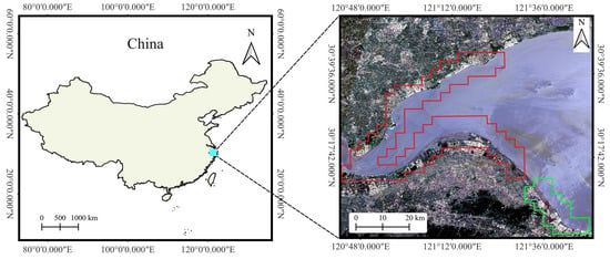
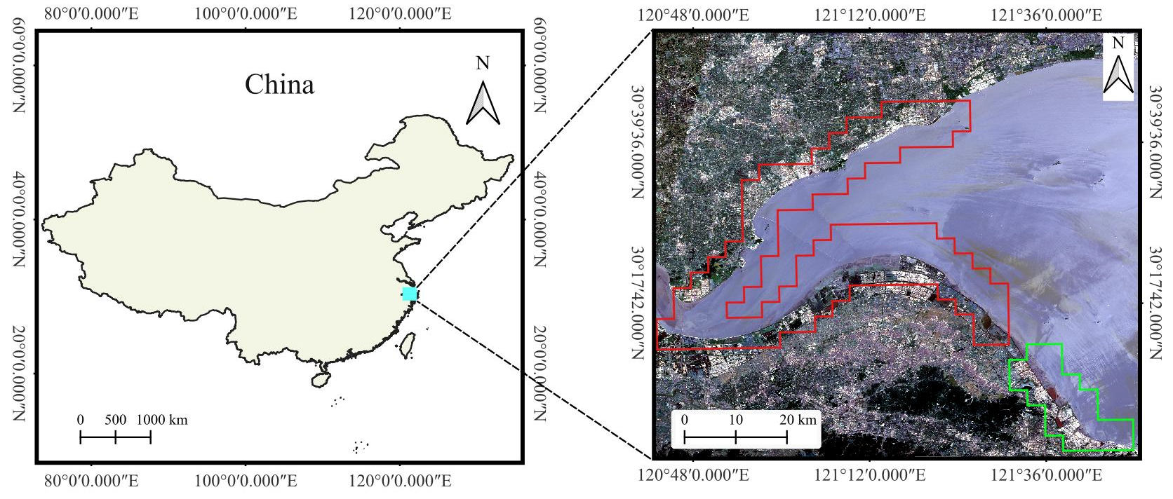
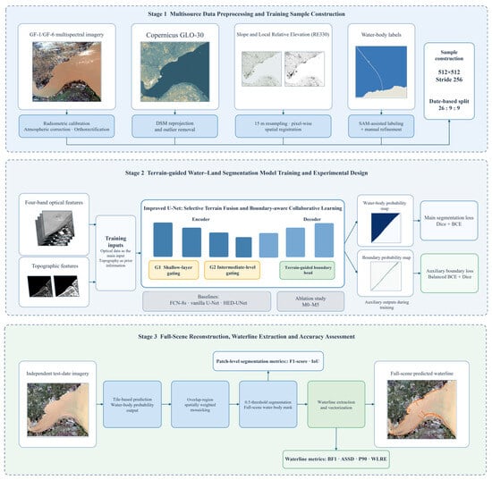
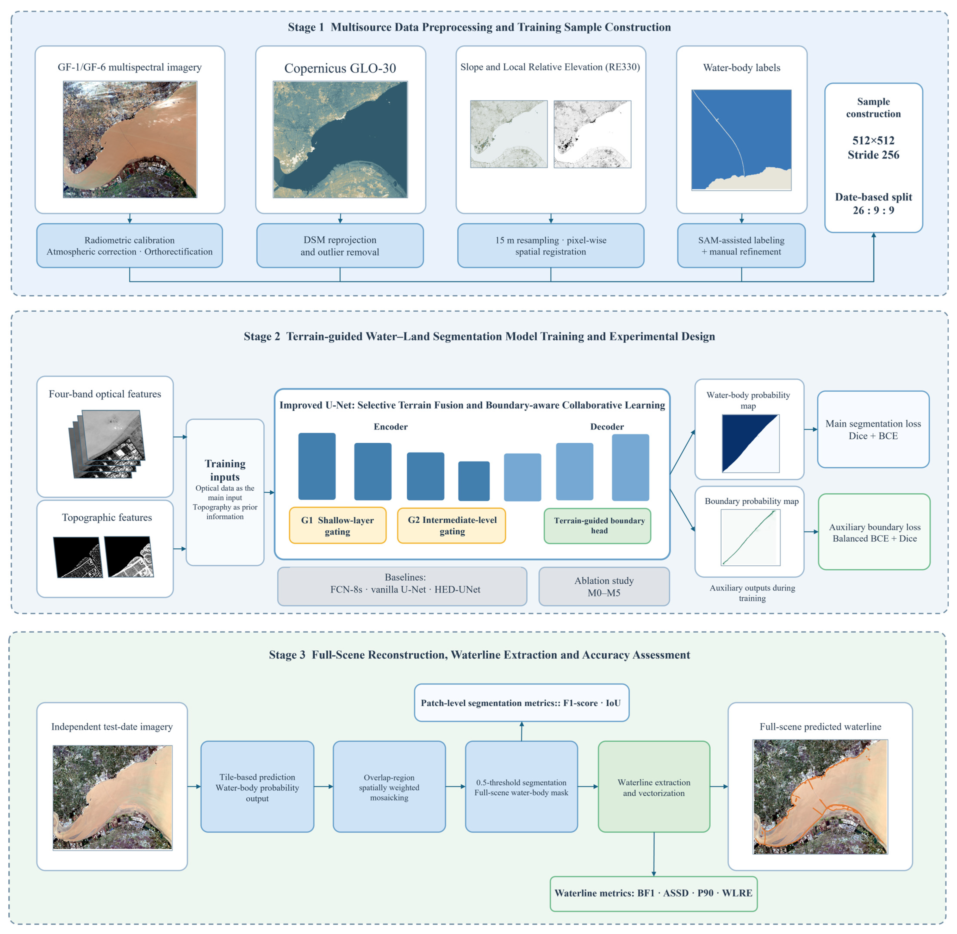
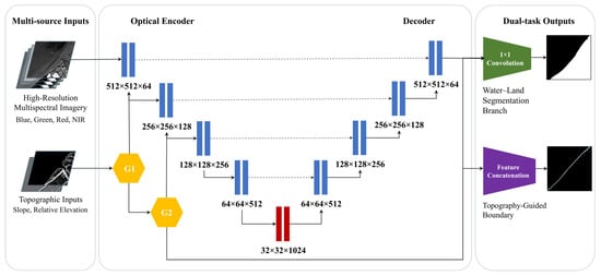
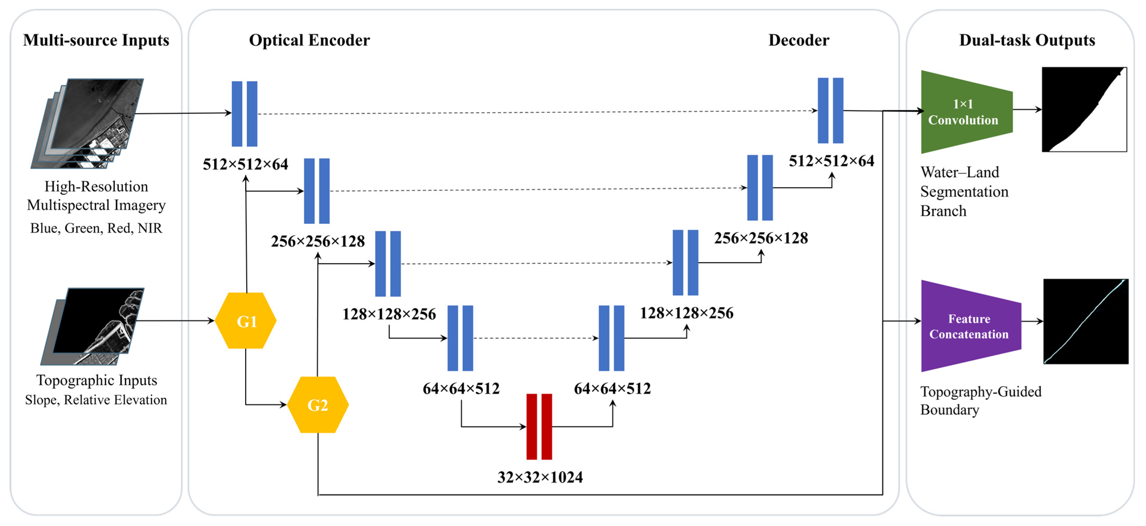
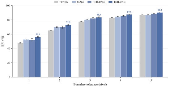
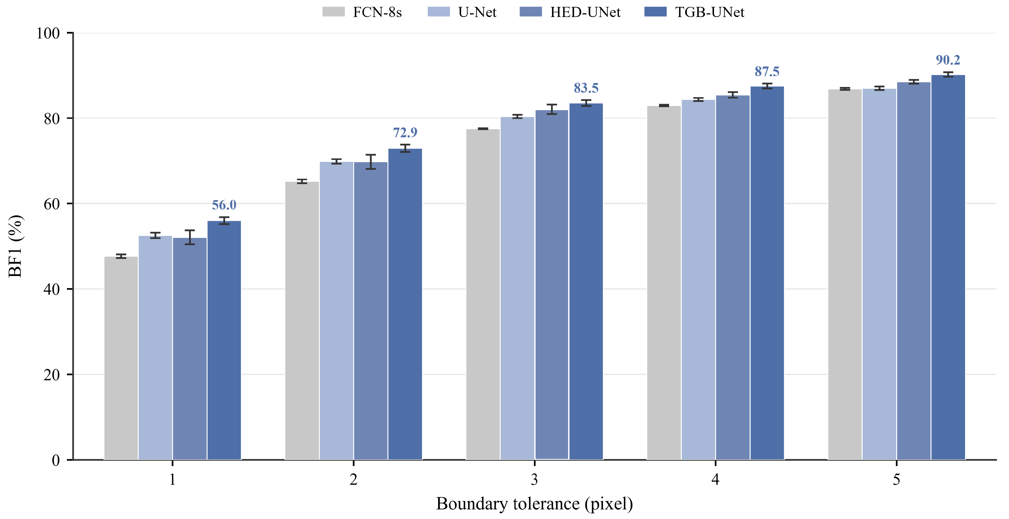
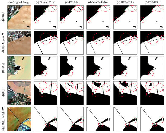
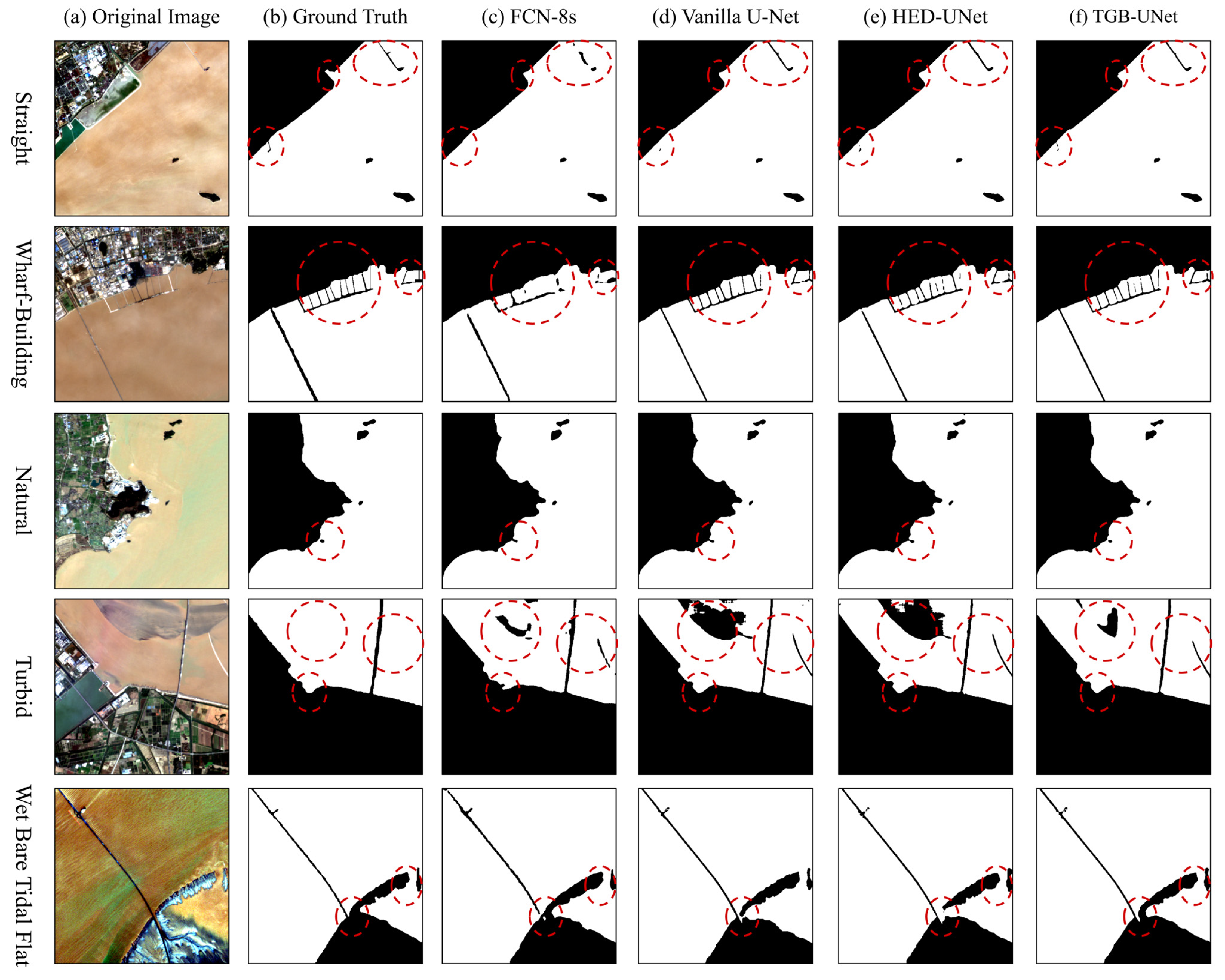
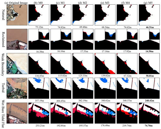
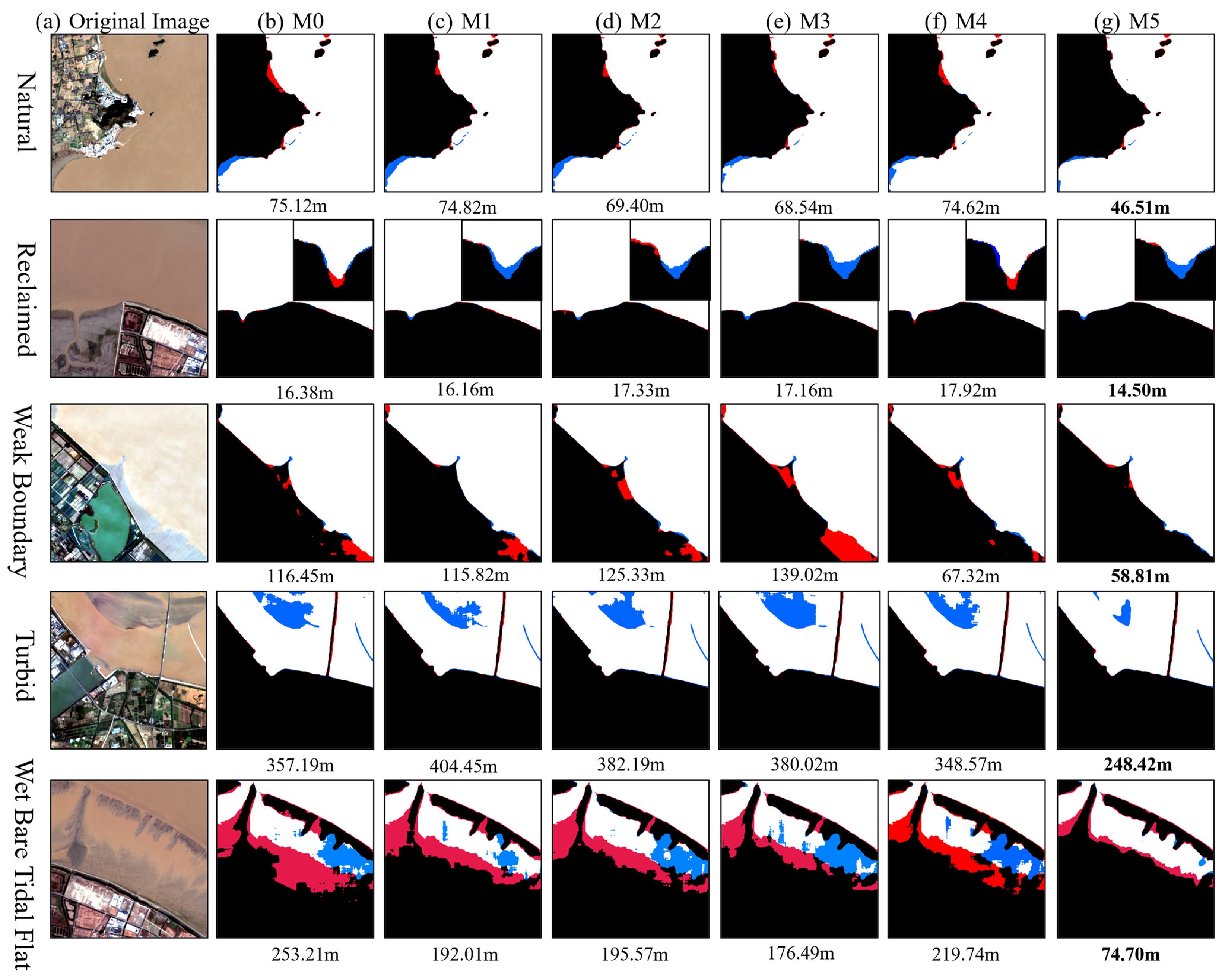
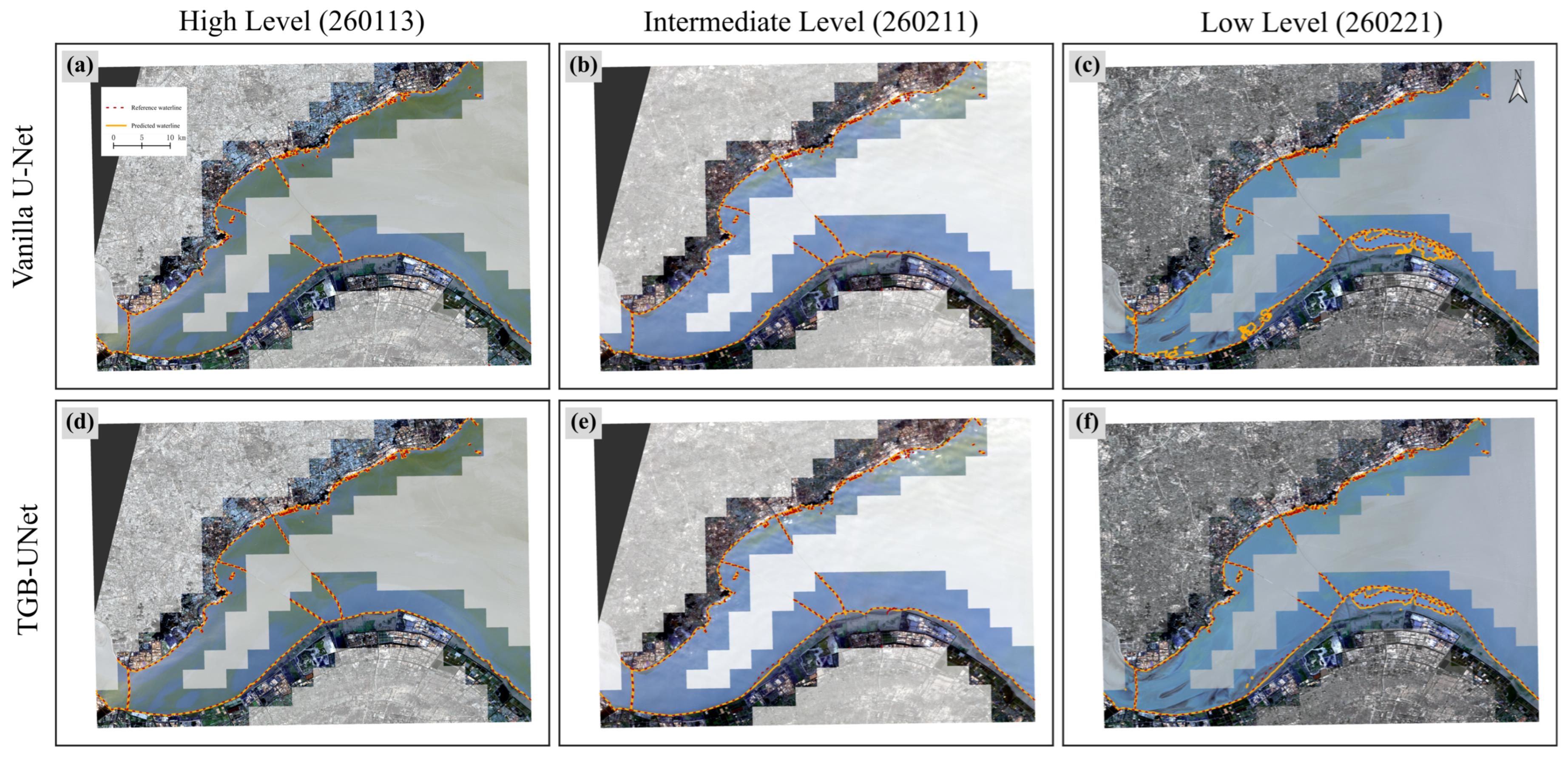
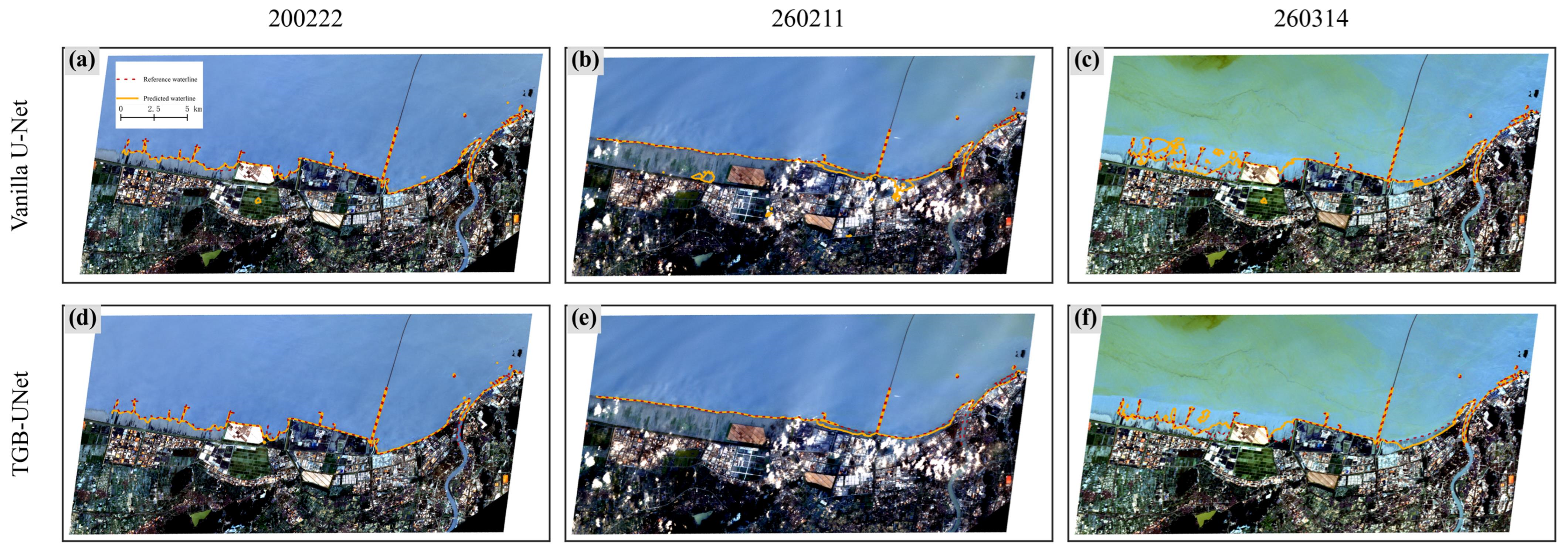

Disclaimer/Publisher’s Note: The statements, opinions and data contained in all publications are solely those of the individual author(s) and contributor(s) and not of MDPI and/or the editor(s). MDPI and/or the editor(s) disclaim responsibility for any injury to people or property resulting from any ideas, methods, instructions or products referred to in the content. |
© 2026 by the authors. Licensee MDPI, Basel, Switzerland. This article is an open access article distributed under the terms and conditions of the Creative Commons Attribution (CC BY) license.