


Abstract
A transient numerical model is developed for air-assisted recovery of methane hydrate through a vertical pipe. The author’s earlier gas-lift approach is extended with conservative solid transport, separate solid momentum, transported particle number, liquid cooling and distinct air and methane budgets. A moving wet domain represents startup to an outlet above sea level. Air–water measurements assess the hydraulic submodel. Hydrate dissociation, shrinkage and cooling remain predictions conditional on closures requiring hydrate-specific validation. A Japan Sea temperature profile from World Ocean Atlas 2023 supplies the external thermal boundary. For a 500 m intake, a 2 m pipe and 13.2 Nm3 s−1 air injection at 300 m, predicted developed liquid delivery is approximately 38.5 m3 s−1, with 1069.4 kg s−1 of hydrate and 103.3 kg s−1 of methane gas. Dissociation increases liquid delivery by approximately 21.9% relative to the nonreactive case and cools the upper liquid by approximately 1.6 K. External stratification produces no appreciable delivery change in this configuration. Freezing-limited sensitivity, profile refinement checks and an explicitly assumed compressor work calculation qualify the thermal, numerical and engineering interpretation. The framework distinguishes startup, throughput and methane product form with explicit air and methane accounting.
1. Introduction
Methane hydrate recovery must accommodate the simultaneous transport and transformation of solid hydrate, water and methane gas. Resource assessments distinguish hydrate occurrence from the amount recoverable by an engineering process [1,2], while hydrate stability links recovery to methane retention and release [3]. For exposed or shallow deposits, fragmented material can be conveyed through a vertical pipe. Matsukuma et al. [4] discuss gas lift as a recovery method in which externally supplied gas and methane released by dissociation jointly support upward transport. The resulting problem requires coupled hydraulic and thermal descriptions.
Air-lift delivery is determined by the balance between the surrounding hydrostatic pressure and the internal multiphase column, including phase slip and pressure losses. Shimizu et al. [5] applied a drift flux model to rare earth-rich mud lifting, and Pougatch and Salcudean [6] developed a numerical model for deep-sea air-lift. Experimental and analytical work by Kassab et al. [7] and the review by Hanafizadeh and Ghorbani [8] establish how gas supply and geometry affect performance. In such systems, the gas input is prescribed and the liquid transport rate is a coupled output.
Cross-section-averaged models are useful for long pipes and operating studies. The distribution parameter and drift velocity introduced by Zuber and Findlay [9] represent nonuniform phase motion. Ishii [10], Hibiki and Ishii [11] and Bhagwat and Ghajar [12] extended relative motion closures across flow conditions and pipe scales. The author’s previous gas-lift study [13] incorporated void fraction-dependent drift, dimensionless pipe diameter, inclined flow and mud rheology. It provides the modelling lineage for the present extension to a dissociating solid phase, specialised here to a vertical pipe and a constant-property liquid.
Recent air-lift research has demonstrated the sensitivity of predictions to flow representation. Bukhari et al. [14] assessed a flow pattern-dependent performance model; Du et al. [15] investigated gas state relations and axial gas–liquid flow; and Gray et al. [16] resolved unsteady three-dimensional structures. Geometry and injection history also matter: Kassab et al. [17] examined bent risers, Wang et al. [18] analysed variable-diameter pipelines, and Li et al. [19] compared continuous and oscillatory injection. These studies motivate explicit specification of compressibility, relative motion and gas supply history when delivery rates are compared.
Solid particles add another inventory and momentum exchange. Takano et al. developed a pressure drop correlation [20] and measured phase velocities [21] for vertical three-phase resource transport. Höhn et al. [22] examined upward air–water–solid flows containing buoyant particles. Their work supports an explicit solid balance: gas holdup alone cannot determine whether hydrate remains. The present formulation therefore retains solid transport even when the gas–liquid closure changes at a high gas fraction.
Hydrate-specific models connect phase change to gas-lift performance. Kidaka and Sugiyama studied three-phase hydrate recovery [23] and subsequently tapered pipes with multiple injection locations [24]. Shimizu and Sugihara combined drift flux transport with hydrate phase change [25] and extended the system treatment to air and methane [26]. These studies establish the relevance of self-generated gas. The present investigation focuses on the sequencing of startup, separate air and methane budgets and the division of recovered methane between gas and solid products under controlled operating changes.
The dissociation closure must identify the mechanism limiting phase change. Kim et al. [27] and Clarke and Bishnoi [28] investigated intrinsic dissociation kinetics, whereas recent coupled modelling also resolved heat transfer and multiphase response [29]. For transported particles, Matsukuma et al. [4] describe a heat transfer-controlled decomposition framework. The Ranz–Marshall [30] and Whitaker [31] correlations, together with established particle flow descriptions [32], relate transfer to particle size and relative velocity. Here, that framework is implemented with an explicitly stated particle heat transfer coefficient. The enhanced transfer observed for HCFC141b hydrate in [4] motivates a sensitivity calculation, rather than an undocumented empirical fit.
External ocean temperature and internal dissociation cooling have different roles. World Ocean Atlas 2023 [33] provides an observationally based thermal boundary for a representative Japan Sea column. Comparing this profile with a uniform exterior, while preserving the same inlet temperature, isolates the wall boundary effect. Startup additionally requires a moving wet domain because the outlet extends above sea level. Geometrical conservation [34] and refinement assessment [35] are therefore included alongside component budgets.
The contribution comprises the transient conservative coupling and its controlled assessment. Matsukuma et al. [4] already described phasewise mass and momentum, heat-controlled dissociation, shrinking particles and engineering wall heat exchange; these are not claimed as new physical laws. Relative to the author’s earlier gas–liquid approach [13], the present implementation introduces an explicitly transported and moving solid inventory, particle shrinkage and conservative decomposition sources. Its distinctive features relative to the thermal framework in [4] are a transported number density linking particle size to solid inventory, separate injected air and generated methane budgets, a geometrically conservative moving wet boundary for startup to an elevated outlet and a matched thermal boundary comparison that isolates external stratification from changes in inlet temperature. Their coupled use resolves the sequence of overflow and product arrival and distinguishes recovered free methane from hydrate-bound methane, without presuming a universal operating optimum.
Section 2 specifies the formulation and numerical procedure. Section 3 separates the hydraulic experimental assessment from thermal and numerical checks. Section 4 compares startup, dissociation, injection, particles and depth, then examines compressor work and engineering constraints. Appendix A reports profile-level refinement.
2. Numerical Model
2.1. Physical Configuration and Modelling Framework
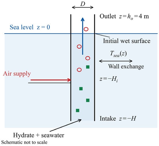
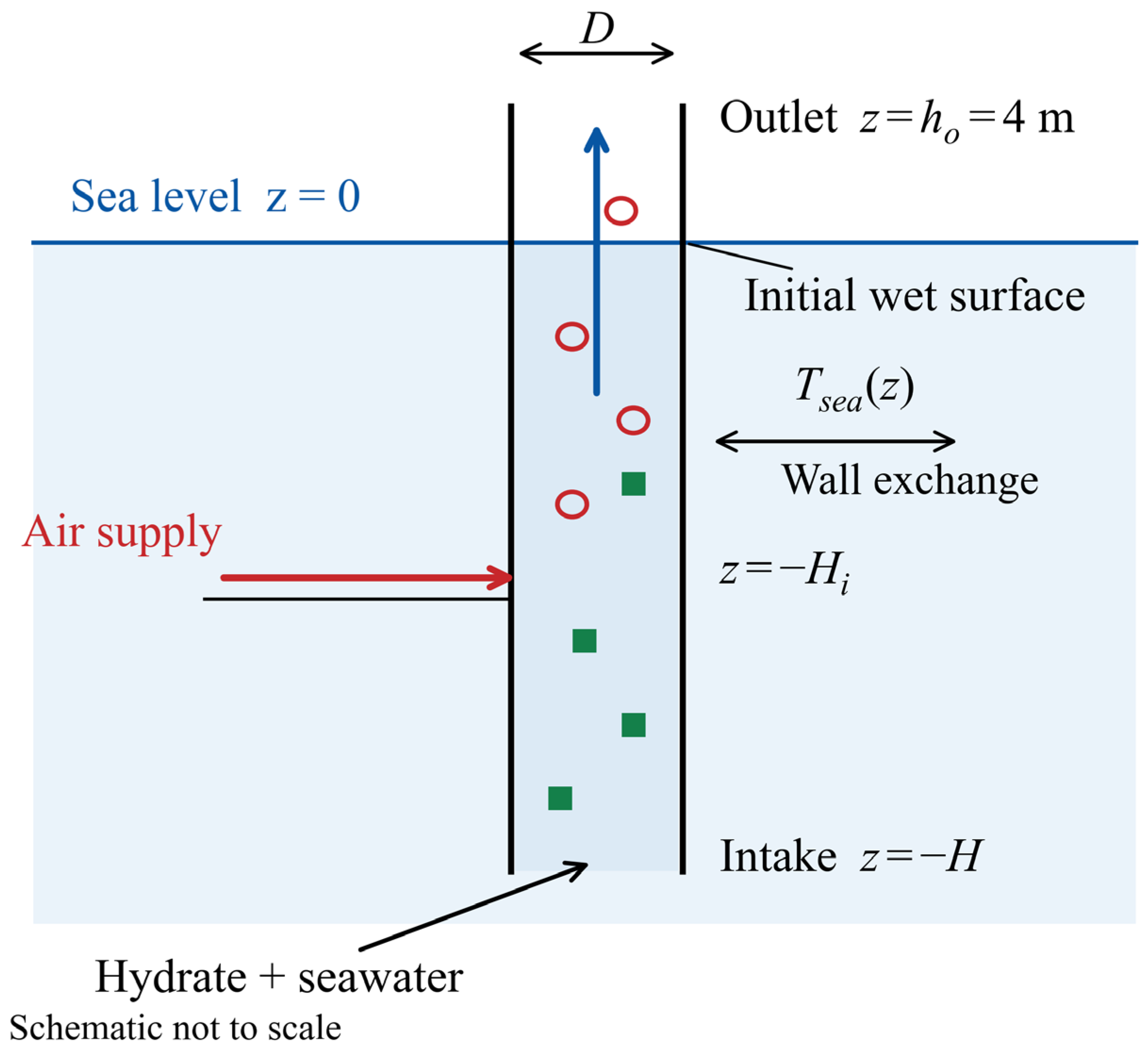
Figure 1 defines a vertical pipe with intake depth H, diameter D and outlet elevation ho = 4 m. The air port is at depth Hi. The coordinate z increases upwards from mean sea level. Initially, clear water fills the pipe to h0 = 0. The bottom opening communicates with the hydrostatic sea and the upper wet boundary with the atmosphere. Hydrate is available at the bottom boundary from the start, but its entering flux is determined by the solved inflow: it is zero during the hydrostatic 0–100 s interval and begins as upward inflow develops after air injection starts. Table 1 lists the reference conditions.
Figure 1.
Physical configuration, initial wet surface, side port air injection and external thermal boundary. The diagram is not to scale.
Table 1.
Reference geometry, material properties and operating conditions.
Normal-volume gas supply is defined at 273.15 K and 101,325 Pa. Latent heat is expressed per unit mass of hydrate.
The phases g, l and s have separate velocities uk and volume fractions αk with a common pressure p. Spherical particles contain pure methane hydrate. Liquid and solid properties are constant; gas follows an ideal air–methane mixture law. Liquid temperature determines gas density and particle heat transfer. Separate gas/solid sensible energy balances, salt transport, dissolved methane, hydrate reformation and an ice phase are not solved. The model is a framework-level transport study; its hydrate-specific closures require validation and its operating cases are not an engineering design.
Air-assisted hydrate lifting follows an existing research route. Matsukuma et al. [4] combined laboratory gas-lift pumping with recovery pipe modelling, while Shimizu and Sugihara [26] explicitly simulated air and dissociation-generated methane in the same hydrate/slurry riser. These studies motivate the present compressed-air configuration and separate gas accounting. Its engineering implementation must manage the potentially flammable inventory through controlled collection and gas–liquid–solid separation at the outlet, methane/oxygen composition monitoring, ignition source control, pressure protection and interlocked isolation and shutdown. These design requirements follow the prevention, detection and control principles used in offshore gas handling [36] and apply across startup, developed flow and shutdown. A gas–liquid–solid separator removes entrained liquid and solids; it does not by itself separate methane from air. Water in the riser and mean outlet composition are therefore not credited as explosion barriers [37]. The calculated gas flow and inventory histories provide the transport inputs for sizing the gas-handling equipment and assessing the operating sequence.
The earlier modelling line [13] is extended with solid inventory and momentum, particle shrinkage, conservative decomposition sources, liquid cooling and gas component accounting. Its inclination and mud rheology terms are not invoked in these vertical, constant-property cases. The current implicit finite-volume implementation is specified below. The thermal source structure follows [4], with an explicit particle heat transfer closure.
2.2. Phase Mass and Gas Component Balances
The cross-sectional area is , and the phase fractions satisfy
For a stationary coordinate, the local mass balances are
Let be the mass of hydrate decomposed per unit bulk volume and time, and let be the corresponding volumetric source of injected air mass. The hydrate formula is taken as , with . Its methane mass fraction is
The mass sources then become
Thus, the dissociation sources sum to zero, and only the imposed air supply adds total mass within the pipe. For a narrow side port, is distributed between adjacent cells with nonnegative weights whose sum is one. Its integral satisfies
Within the total gas fraction, denotes the air partial volume fraction, so that is the methane partial volume fraction. Under the common-pressure, common-temperature ideal-mixture approximation,
where and are gas component masses per unit bulk volume. Their conservation equations are
In practice, total gas mass and air mass are advanced; methane follows from their difference. The gas density used in the momentum equation is
Gas holdup maps display air and methane together. Separate component accounting supplies methane partial pressure and product rates.
2.3. Momentum Exchange and High Gas Fraction Closure
Writing , the conservative phase momentum balances are
Here, is interfacial drag, is wall resistance and is the momentum carried by mass transfer or injection. For dispersed gas and hydrate particles, the drag relative to the liquid is
The drag coefficient is evaluated from the Schiller–Naumann-type spherical particle expression, with a constant high-Reynolds-number floor [32],
The Stokes limit is implemented through the product , avoiding division by a vanishing slip velocity. The gas diameter is fixed in the dispersed regime, whereas the hydrate diameter evolves. Liquid wall resistance is , and . The Fanning friction factor uses the laminar value and the turbulent value , with and a smooth interpolation over . An additional inlet loss is used only for the laboratory calibration described in Section 3.1; it is zero in the deep-water cases.
The dispersed gas momentum closure is progressively replaced when the total gas fraction rises from 0.25 to 0.30. Define , the gas fraction within the gas–liquid part, and . The high-holdup relation is
The principal drift parameters are
At very high , an annular-form extension following the drift flux modelling tradition [10] regularises the gas-rich limit. With ,
Both transitions use , with clipped to . Equations (13) and (14) are blended over . These bounds are engineering choices. The combined gas–liquid momentum balance is retained, and solid mass and momentum remain active at every gas fraction.
The mass transfer momentum terms use the solid velocity for material released by decomposition:
The axial injection velocity is set to zero for the side port input. At a vanishing solid inventory, its otherwise indeterminate auxiliary velocity is set to the liquid velocity when the previous accepted face mass is below kg m−3. This treatment regularises the momentum equation without deleting solid mass or suppressing transport of newly entering hydrate.
2.4. Heat-Controlled Hydrate Dissociation and Particle Shrinkage
The decomposition model assumes that the hydrate surface is at its local equilibrium temperature and that sensible heat from the surrounding liquid supplies the dissociation enthalpy. This is the heat-controlled framework discussed in [4]. Because the injected gas is air, the implemented equilibrium pressure is the methane partial pressure, . The empirical equilibrium–temperature relation is
Temperature is in kelvin and pressure in pascals. The methane partial-pressure substitution is an ideal-mixture approximation for the air-assisted case; it does not treat injected air as methane. The 100 Pa floor regularises the logarithm in nearly methane-free gas. This correlation is not a salinity-dependent hydrate/ice equilibrium calculation, and its use in the coldest cells is a modelling assumption rather than validated saline phase behaviour.
For a local spherical particle population, the interfacial area per unit bulk volume is . The heat flux consumed by dissociation and the mass source are
Here, kJ kg−1 is defined per unit mass of decomposed hydrate, not per unit methane mass. The effective diameter is . The particle heat transfer coefficient is specified by
Equation (18) is the Ranz–Marshall form [30], with Ch = 1. Its Reynolds number uses the regularised slip [(us − ul)2 + (10−4 m s−1)2]1ᐟ2. The enhanced HCFC141b transfer discussed in [4] is not used as a fitted methane–hydrate correlation; Ch = 2 is tested separately. Equation (17) prescribes a finite heat transfer-limited rate, not instantaneous equilibrium of the bulk mixture. Cooling reduces its driving force, but intrinsic reaction resistance, an ice-layer barrier and morphology-dependent self-preservation are absent. Experiments show that low-temperature dissociation depends on salinity as well as temperature [27,28,38,39]; these results motivate qualification of the closure, not an uncalibrated kinetic correction.
Particle shrinkage is obtained from a transported number density ,
The inlet number density is 6αs,in/(πds,03). Fragmentation, aggregation and size distributions are excluded. Solid mass and number determine particle shrinkage independently of the gas closure transition. For pure hydrate, Equations (17) and (19) give Dsds/Dt = −2hs[Tl − Teq]+/(ρsLh), consistent with the diameter loss relation in [4]. Here, Ds/Dt = ∂/∂t + us∂/∂z is the material derivative following a solid particle, and [x]+ = max(x, 0) is the positive part; the subscript “+” does not denote a phase or an additional derivative.
2.5. Liquid Temperature and External Heat Exchange
The liquid temperature is advanced using the constant-property approximation
Equation (20) includes liquid advection, wall exchange and latent cooling, following the constant-property liquid temperature approximation in [4]. It is not a conservative total-mixture enthalpy equation; phase-specific sensible enthalpy transfer, gas expansion work and dissolved methane enthalpy are excluded. Consequently, comparisons of its source magnitudes are not presented as a closed plant or mixture energy budget. For the submerged wall,
The inside heat transfer coefficient uses , with and . The external coefficient uses , and . These pipe wall closures follow the engineering heat transfer treatment in [4]. The wall thickness and conductivity are 0.012 m and 16 W m−1 K−1, respectively, and the external water speed is 0.1 m s−1.
Above the sea surface, , with W m−2 K−1. Cells crossing receive a length-weighted combination of water-side and air-side exchange. The sea surface temperature is used as a common air temperature proxy in the controlled comparison. The external temperature profile is sampled at the instantaneous physical depth, so that the thermal boundary does not move with the mesh.
Equation (20) neglects axial molecular conduction because longitudinal heat transport is dominated by advection at the present scales. This is consistent with the hydrate gas-lift liquid temperature equation of Matsukuma et al. ([4], Equation (3)). Using the stated liquid properties, the thermal diffusivity is al = kl/(ρlcp,l) ≈ 1.4 × 10⁻⁷ m2 s−1. The reference superficial liquid velocity Ql/A ≈ 12.3 m s−1 gives PeD = (Ql/A)D/al ≈ 1.8 × 10⁸ and PeH = (Ql/A)H/al ≈ 4.5 × 10¹⁰. The axial conduction-to-advection ratio scales as Pe−1; it is approximately 5.5 × 10⁻⁹ even when the shorter pipe diameter is used as the temperature variation length. During startup, the prescribed initial liquid temperature is uniform, and the molecular diffusion distance over the first 100 s is only approximately 3.7 mm. Thermal conductivity is retained in the particle and wall heat transfer coefficients in Equations (18) and (21). Thus, the approximation concerns axial bulk conduction, while the wall heat input and particle-scale heat transfer remain explicitly represented.
For the additional freezing-limited sensitivity, the original heat transfer demand q* from Equation (17) is bounded by the heat available above an assumed fixed threshold Tf = −1.9 °C. Write the discrete liquid temperature row as Tj − Tjn + Δt{aj(Tj − Tᵤp,j) − (qw,j − qdec,j)/(ρlcp,l)} = 0, with aj = |ul,j − wj|/Δz and the upwind temperature Tᵤp,j evaluated at the new time level. The consistent source limitation is
qav,j = ρlcp,l[(Tjn − Tf)/Δt + aj(Tᵤp,j − Tf)] + qw,j,
qdec,j = min(q*j, max(qav,j, 0)), Γj = qdec,j/Lh.
When the cap is active with qav,j ≥ 0, substitution into the temperature row gives (1 + Δt aj)(Tj − Tf) = 0. Thus, the threshold follows from the solved thermal equation, without overwriting the accepted temperature or adding artificial heat. The same limited Γ is used for hydrate loss, methane and water generation and mass transfer momentum. Particle shrinkage still follows the remaining mass and transported number. This construction is consistent with Equation (20), not a new total-mixture enthalpy balance. The fixed threshold is a diagnostic sea-water-scale assumption [40], not an inlet salinity measurement or a local pressure- and salinity-dependent freezing calculation.
2.6. Boundary Conditions and Numerical Procedure
The bottom pressure is pb = patm + ρsea gH. The wet surface pressure is atmospheric, including the small air column hydrostatic correction between sea level and h. Inlet liquid temperature, hydrate volume fraction and particle diameter specify the incoming material, whereas the velocities and mass fluxes are solved from the pressure-coupled system. For positive bottom inflow, the hydrate mass flux is Aρsαs,inus,in. The inlet is not a prescribed solid feed rate boundary. Upwinding selects the reservoir composition on inflow and the interior composition on outflow. The pre-injection hydrostatic state has zero net intake. During surface rise, liquid moves with the wet boundary and solids remain below it. Liquid and solid outflow are permitted after the surface reaches the outlet; gas can vent earlier. The uncomputed headspace is not assigned a liquid or solid volume fraction.
For a standard-volume air supply ,
The normal state is TN = 273.15 K and pN = 101,325 Pa. The reference supply is 13.2 Nm3 s−1, equivalent to approximately 17.1 kg s−1 of air, and t0 = 100 s and τᵣ = 60 s. The supply is motivated by the scale of the 300 m injection depth case in Figure 10 of [4] and is a reference input, not a previously established optimum for this three-phase model.
The wet column uses a staggered finite-volume arrangement: pressure, fractions, temperature and particle number are cell-centred, while velocities are face-centred. The mesh coordinate is z = −H + ξ[H + h(t)], and its velocity is w = ξ dh/dt. For phase mass density mk = αkρk, Equation (25) applies the backward Euler method (also called the implicit Euler method):
Here, and . Retaining the old and new cell volumes enforces geometric conservation [34]. Upwind phase fractions and particle number densities are used in the advective fluxes. Gas molar density is interpolated to interior faces and evaluated at the imposed reservoir pressure on boundary faces. Momentum is discretised on staggered dual volumes, while temperature advection uses the liquid velocity relative to the mesh. The wet surface update is .
The coupled nonlinear equations are solved by damped Newton iterations using a sparse finite-difference Jacobian. The reference maximum time step is 1 s, the target advective Courant number is 1.5 and the scaled nonlinear residual tolerance is . Time steps are reduced after an unsuccessful iteration and aligned with injection events and output times. The injection mass is integrated exactly over each step of the linear ramp. Profiles are stored every 2 s; this output interval is independent of the internal adaptive time step.
Within the 0.25–0.30 gas fraction interval, the discrete gas row is blended between its scaled momentum residual and the drift residual. Specifically, the row is , with s and face-averaged fractions. The combined gas–liquid momentum row remains . This documents the actual discrete transition, including its residual scaling, instead of assigning an abrupt physical transition at 30% gas.
2.7. Transport and Recovery Indicators
The phase delivery rates are obtained from boundary mass fluxes, not from a prescribed outlet velocity. Liquid delivery is . Hydrate and gaseous methane delivery are reported separately. Their combined methane-equivalent delivery is
This indicator counts methane crossing the upper boundary in free-gas or hydrate-bound form. It assumes both outlet streams are available for collection and does not represent downstream separation efficiency. At a developed state, the solid retention ratio is Rs = ṁs,oᵤt/ṁs,in and the gaseous product share is fm = ṁm,oᵤt/ṁeq. Specific air use is defined by
Specific air use has units Nm3 kg−1 of methane-equivalent product. It is distinct from compressor energy per unit product, estimated separately in Section 4.5. The transient decomposition fraction is
with the solid inventory included when checking the corresponding mass budget. Developed-state averages use the final 200 s of each completed run. Liquid settling time is the first saved time after which delivery remains within 2% of its final window mean for the rest of the run. These definitions separate the beginning of overflow from the later establishment of a stable transport rate.
3. Hydraulic Assessment and Thermal Model Checks
3.1. Comparison with Air–Water Experiments
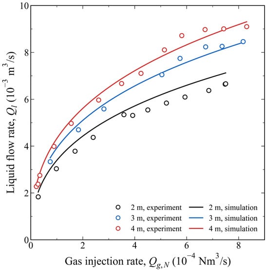
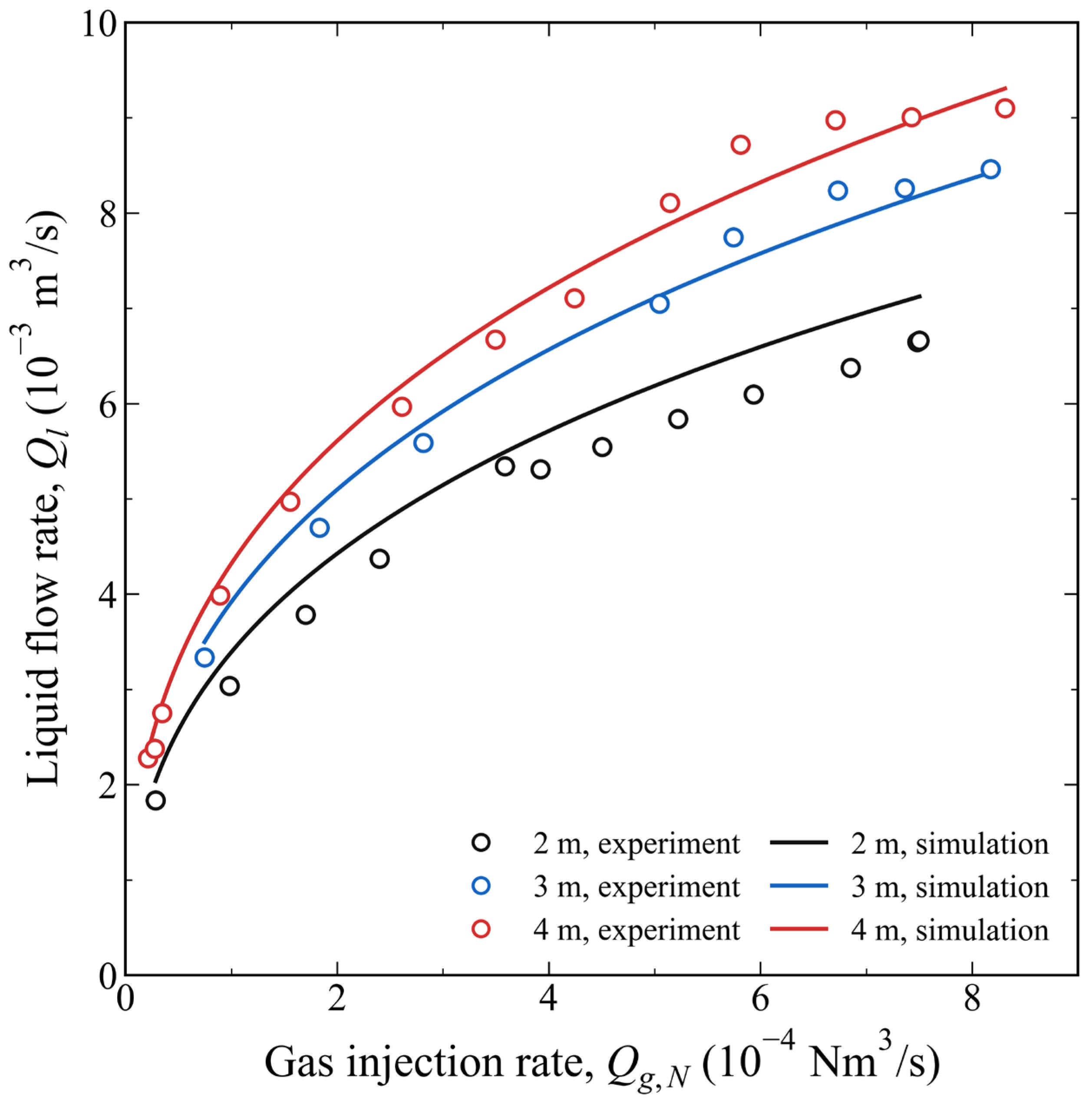
Figure 2 compares the model predictions with the experiments. The hydraulic comparison uses digitised liquid delivery measurements from Figure 4 of [4]: 12 points at 2 m injection depth, 8 at 3 m and 13 at 4 m. An unresolved near-origin 3 m marker is excluded before comparison. Each retained experimental air input and injection depth is supplied to the model; measured liquid delivery is not imposed.
Figure 2.
Comparison of numerical predictions with experimental liquid delivery measurements at injection depths of 2, 3 and 4 m. Hollow circles: experimental data digitised from Figure 4 of Matsukuma et al. [4], published by The Japanese Society for Multiphase Flow, 2022. Solid curves: numerical predictions from the present study. The common loss coefficient was calibrated using the 4 m experimental series.
The laboratory calculation uses a 5.5 m water column, 0.1 m pipe diameter, 293.15 K temperature, liquid density 998.2 kg m−3 and viscosity 0.001002 Pa s. The 3 mm diameter is the assumed dispersed gas bubble diameter used in the gas–liquid drag closure; it is not an injection nozzle diameter and is not a measured evolving bubble size distribution. Gas supply is converted at 273.15 K and 101325 Pa. With hydrate and decomposition disabled, a steady reduction retains the dispersed gas–liquid momentum equations. The boundary assumes an ideal fully submerged hydrostatic supply.
An effective loop loss coefficient K ≈ 2.36 is calibrated using only the 4 m series and then held fixed for the 2 and 3 m comparisons. Thus, 4 m is calibration and the other depths are held-out checks. This coefficient is not transferred to the deep-water pipe. The experiments assess laboratory air–water pumping, not methane hydrate dissociation, particle shrinkage, liquid cooling or full-scale high-holdup flow. The hydrate-related results below are model predictions conditional on assumptions requiring hydrate-specific validation.
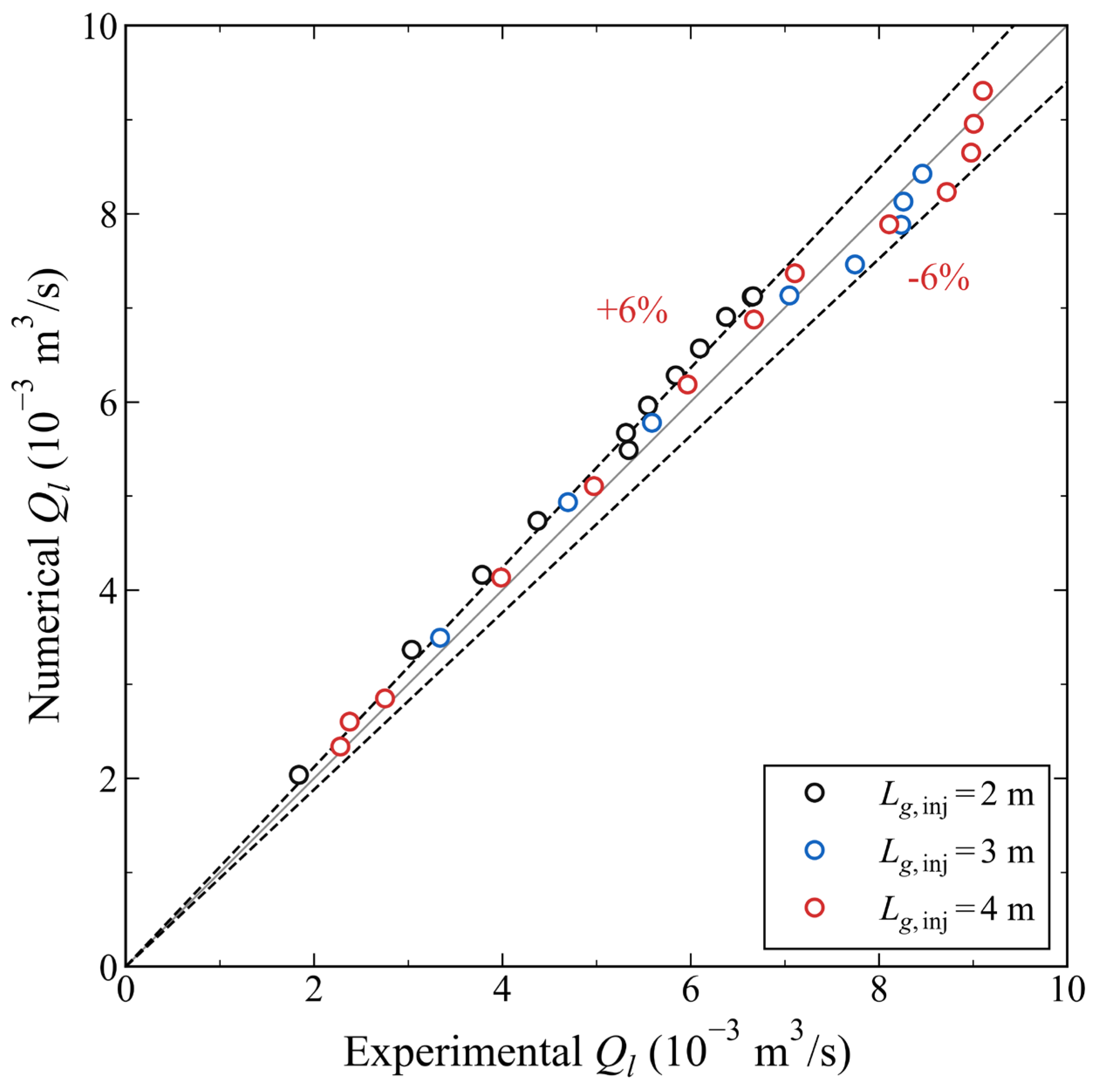
Figure 3 compares each measured liquid delivery with the prediction for the same input. Equality and reference lines show pointwise discrepancies. At 3 m, all 8 points lie within the reference band. At 4 m, 12 of 13 points do so. At 2 m, only 1 of the 12 points is inside the band, with the model overpredicting liquid delivery by approximately 2.8–11.0%. Thus, the comparison captures the depth dependence but retains a systematic shallow injection bias. Digitisation and boundary assumptions contribute uncertainty, but their separate effects cannot be identified from these data.
Figure 3.
Pointwise predicted and measured liquid delivery at matched air inputs, with hollow markers for experimental cases, dashed ±6% discrepancy lines and the 4 m series identified as calibration.
The heat transfer and dissociation literature motivates the chosen closure but supplies no matched experimental validation of the full present system. In particular, the HCFC141b particle measurements discussed in [4] are not methane hydrate flow data. Recent hydrate gas-lift studies [23,24,25,26] provide numerical context, not independent experimental confirmation of the present product rates. A discriminating validation would measure hydrate mass loss or particle size evolution, methane release and liquid temperature together with the hydraulic response under matched pressure, salinity and feed conditions.
3.2. Japan Sea Temperature Data and Controlled Comparison
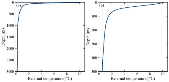
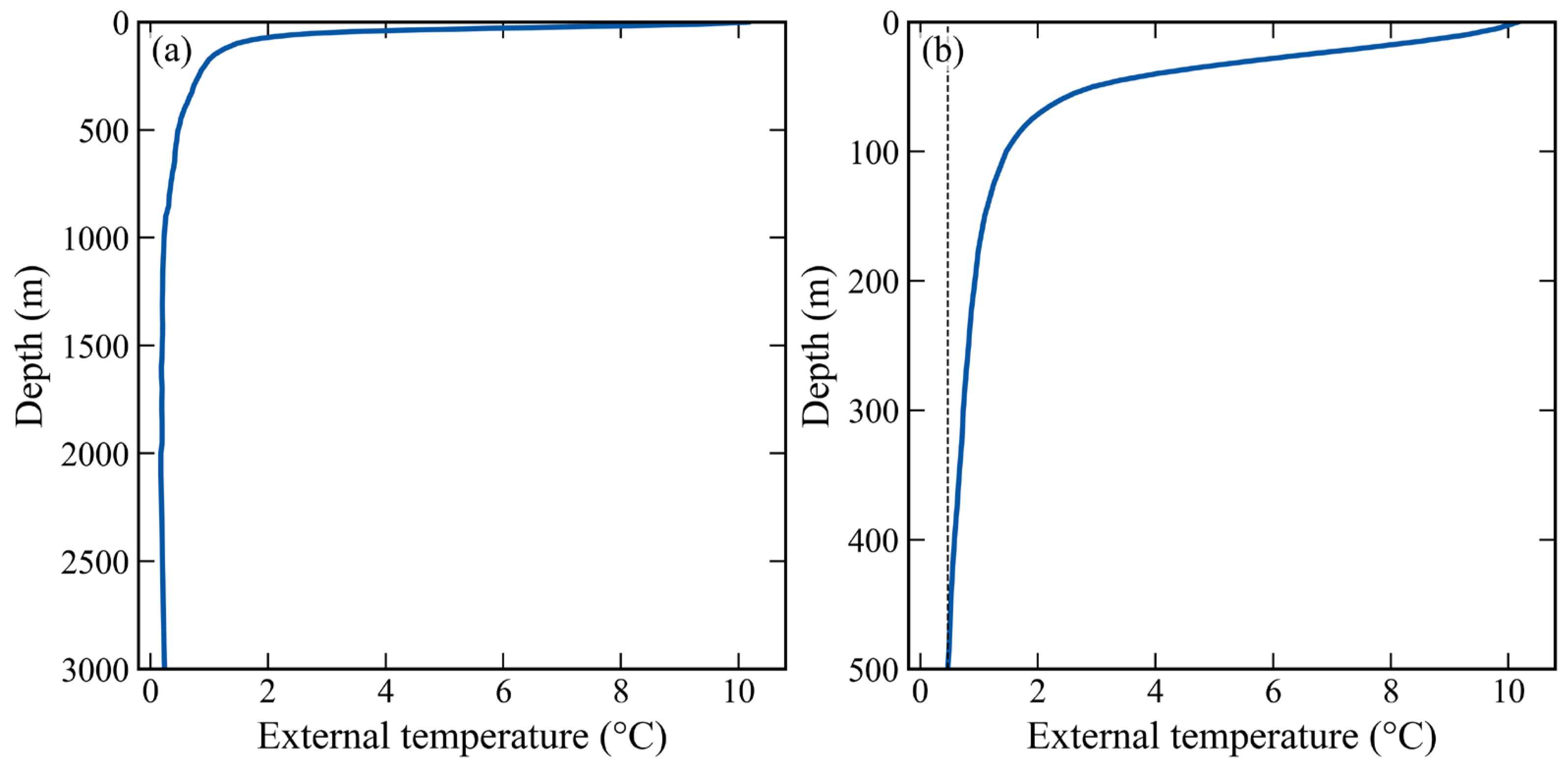
The external boundary uses the annual WOA23 objectively analysed in situ temperature field [33] at 0.25-degree resolution for the 1955–2022 decadal average climatology. A Japan Basin column at 41.125° N, 135.125° E supplies 77 valid depths between 0 and 3000 m. Temperatures are linearly interpolated without deeper extrapolation.
Figure 4 shows a warm upper ocean and cold deep water. Temperatures are approximately 10.2 °C at the surface, 0.7 °C at 300 m, 0.5 °C at 500 m, 0.2 °C at 1000 m and 0.2 °C at 2000 m. The small deep-water inversion is retained in the WOA23 input data. This is a representative environmental profile, not a production site survey; truncation at 500 m does not identify the actual seabed depth at these coordinates.
Figure 4.
Annual WOA23 temperature at 41.125° N, 135.125° E for (a) the available 0–3000 m column and (b) the baseline 0–500 m interval, with the uniform exterior temperature shown by a dashed line.
The controlled pair uses identical geometry, injection, particles and wall properties. In both calculations, the liquid initially inside the pipe and the liquid subsequently entering at the bottom have the same specified temperature of approximately 0.5 °C. Only the submerged external temperature differs: the WOA23 profile or a uniform exterior at the intake temperature. Above-water exchange is identical. The initially uniform internal temperature is an imposed startup condition.
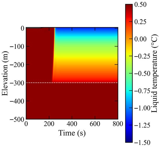
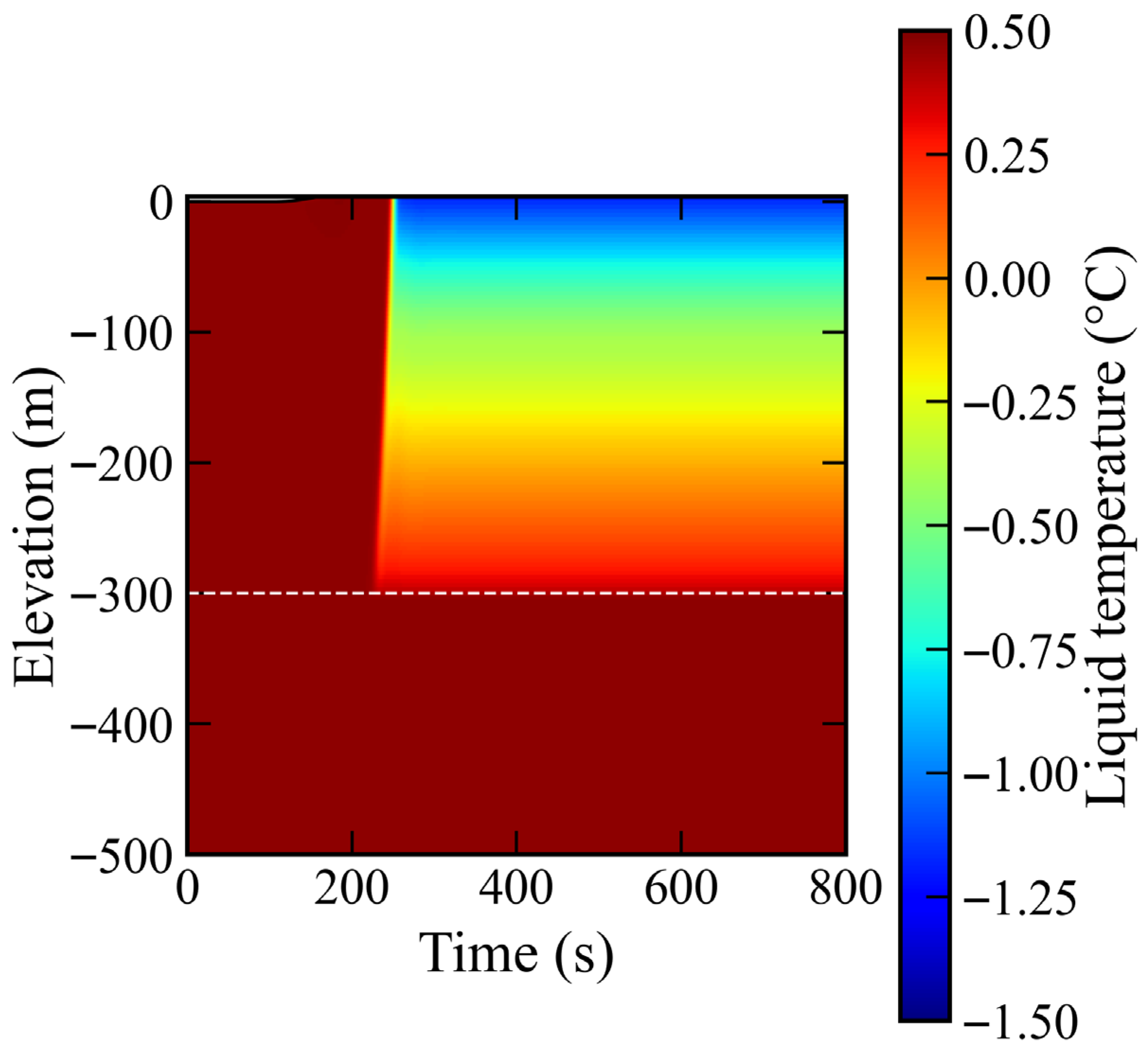
In Figure 5, a cooling region follows the advancing hydrate inventory. The minimum saved liquid temperature and developed top-cell temperature are both approximately −1.2 °C, about 1.6 K below the inlet temperature. These are ice-free model predictions. A negative Celsius temperature alone does not imply sea-water freezing; the onset depends on salinity and pressure [40]. Bulk temperature above a nominal sea-water freezing point also does not exclude local icing at a colder, freshened particle surface.
Figure 5.
Liquid temperature evolution for the 500 m baseline with the Japan Sea exterior, the −300 m air port marked by a dashed line and the wet surface marked by the upper black line.
Table 2 shows no appreciable operating response to the external temperature profile. Both calculations give the same liquid delivery, hydrate and methane deliveries and top-cell temperature when reported to one decimal place. Specific air use changes negligibly.
Table 2.
Controlled external temperature comparison. Delivery and top-cell temperature are averaged over 600–800 s.
Calculated results are reported to one decimal place; scaled units are used for small quantities.
The heat quantities in Table 2 are integrated wall heat transfer rates (powers), not local heat flux densities. WOA23 increases wall input from 99.5 to 316.9 kW, a factor of 3.2. The additional 217.4 kW is approximately 6.3 × 10⁻²% of the 346.7 MW latent sink. Advected liquid sensible cooling supplies the dominant thermal contribution in Equation (20), explaining the weak throughput response to external stratification in this large-diameter, high-throughput case.
3.3. Conservation and Discretisation Checks
Inventories are checked against integrated boundary fluxes and sources for each phase and gas component. The moving-domain scheme preserves hydrostatic liquid before injection and prevents liquid discharge before overflow. For both thermal control cases, the maximum cumulative phase mass discrepancy divided by initial pipe mass is approximately , with volume fractions close to unity at roundoff.
Table 3 compares the 80-, 160- and 320-cell solutions at the same post-startup time of 300 s. Relative to 320 cells, the 160-cell liquid and methane-equivalent deliveries differ by approximately 0.5%, and top-cell temperature differs by about 1.1 × 10⁻² K. Halving both the maximum time step and target Courant number on 160 cells changes liquid delivery by approximately 0.3% and methane-equivalent delivery by less than 1.0 × 10⁻²% at that time; over 0–300 s, the integrated absolute liquid flow difference is approximately 1.1% of the baseline cumulative liquid delivery. Appendix A adds full axial profile comparisons and norms so that the assessment does not rely only on outlet quantities. Although domain-mean profile discrepancies decrease on refinement, the maximum gas fraction discrepancy remains approximately 0.1 in the outlet cell for 160 versus 320 cells. The narrowing outlet holdup feature is therefore still mesh-sensitive, and the throughput comparison does not establish uniform pointwise convergence. These checks quantify discretisation sensitivity; they do not establish depth-specific grid independence or physical accuracy at the displayed number of digits.
Table 3.
Spatial and temporal refinement: the common post-startup state at 300 s.
The time-refined calculation halves the maximum time step and target Courant number. All comparisons use identical physical inputs and the same time; these are not final window averages.
First-order upwind transport and the backward Euler method are formally first order in space and time for smooth solutions. The clipped cubic smoothstep is continuously differentiable at its transition endpoints; it does not introduce a jump in the blended closure. Positive part/max operations are continuous but have derivative changes, while the vanishing inventory velocity regularisation and overflow event are active set changes. These features and the cell-distributed injection can reduce smoothness and affect Newton convergence. Coupled adaptive space/time refinements are reported as sensitivity checks, and profile comparisons are provided in Appendix A. Cell-scale fronts are not interpreted as resolved physical interfaces.
4. Numerical Results and Discussion
4.1. Transient Evolution of the Reference Case
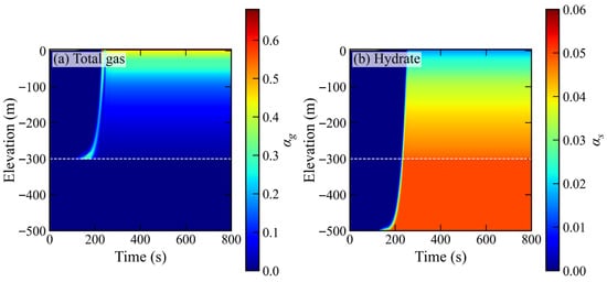
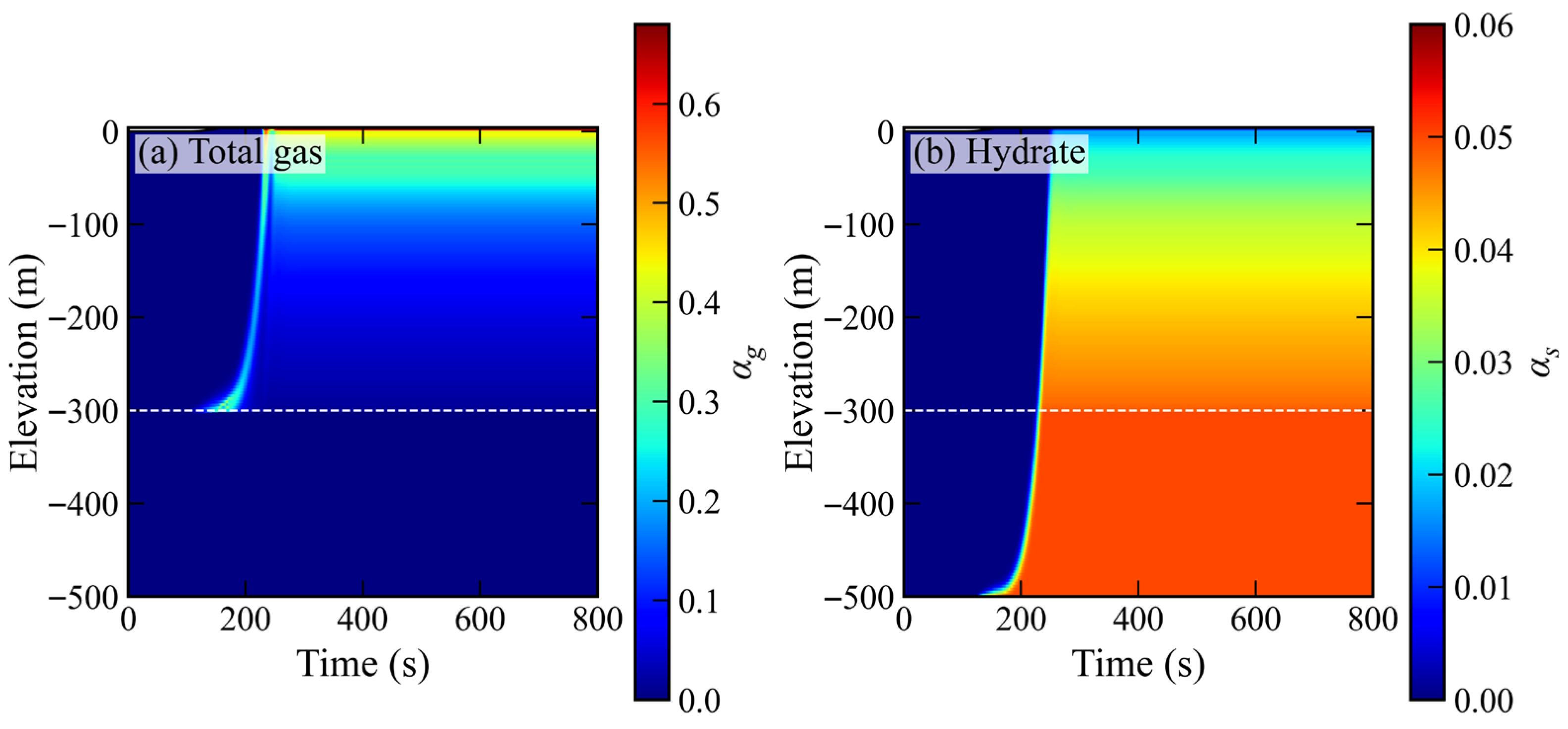
The reference calculation separates hydraulic startup from the arrival of recoverable hydrate. Initially, the pipe contains clear water up to sea level. Air injection begins at 100 s, and the prescribed supply increases linearly until 160 s. Figure 6 shows the subsequent propagation of gas and solid inventories. The total gas fraction includes both injected air and methane generated inside the pipe. A gas-rich band develops above the air port, while the incoming solid population travels from the bottom opening towards the outlet. The increasing gas fraction towards the upper end reflects the combined effects of gas addition, pressure reduction and phase slip.
Figure 6.
Baseline evolution of (a) total gas fraction (air plus methane) and (b) solid hydrate fraction, with the air port dashed and the wet surface elevation shown in black.
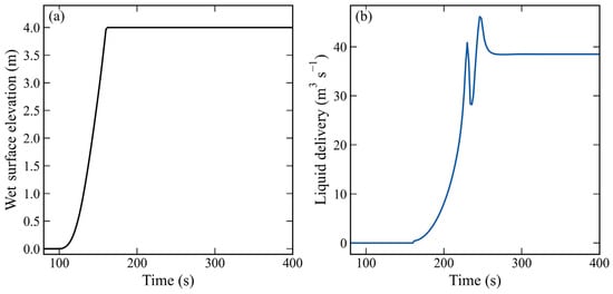
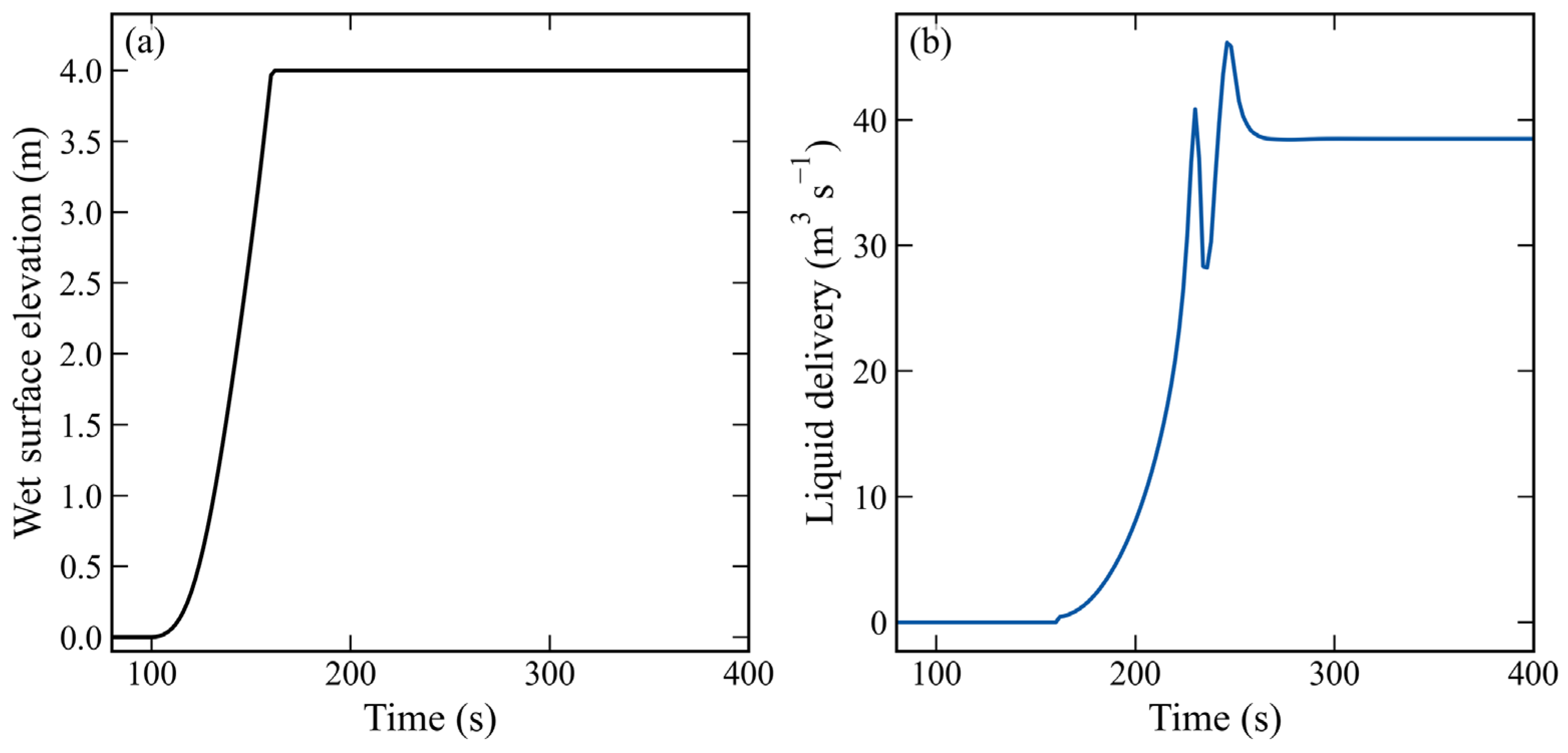
Figure 7 shows wet surface rise and liquid delivery establishment. Overflow begins at approximately 160 s after the surface rises through the 4 m section above sea level. Using 1% of each final window component delivery as the arrival threshold, air, methane and solid hydrate appear at the outlet at approximately 226, 244 and 246 s, respectively. These diagnostics use profiles saved every 2 s. Liquid delivery remains within 2% of its final mean after approximately 258 s. Thus, overflow of the initial water inventory precedes significant hydrate production. A fixed, already liquid-filled pipe extending to the elevated outlet would omit this part of startup.
Figure 7.
Baseline (a) wet surface elevation and (b) liquid delivery histories for air injection starting at 100 s and reaching its prescribed plateau at 160 s.
Initial overflow primarily discharges water already present near the upper end. Incoming hydrate arrives later because of transit and reaction along the wet column. Product accounting therefore accumulates only methane and hydrate that cross the outlet, distinguishing startup storage from recovered material.
The developed reference flow delivers approximately 38.5 m3 s−1 of liquid, 1069.4 kg s−1 of hydrate and 103.3 kg s−1 of methane gas. Methane-equivalent delivery is approximately 246.7 kg s−1, with about 41.9% in free-gas form. Approximately 58.1% of entering hydrate remains solid at the outlet. During 0–800 s, the integrated decomposition fraction is approximately 39.9%; its difference from the developed fraction reflects startup and hydrate still stored in the pipe. The prescribed inlet fraction fixes the entering composition, while solid mass intake remains coupled to the predicted velocity.
Axial pressure reduction, gas expansion and particle shrinkage jointly determine the outlet response. The top-cell hydrate diameter is approximately 8.4 mm, compared with 10 mm at entry. Since particle mass scales with diameter cubed, this reduction represents substantial dissociation while retaining a solid product.
4.2. Coupling of Dissociation, Cooling and Gas Lift
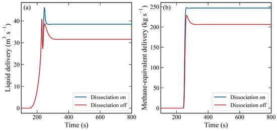
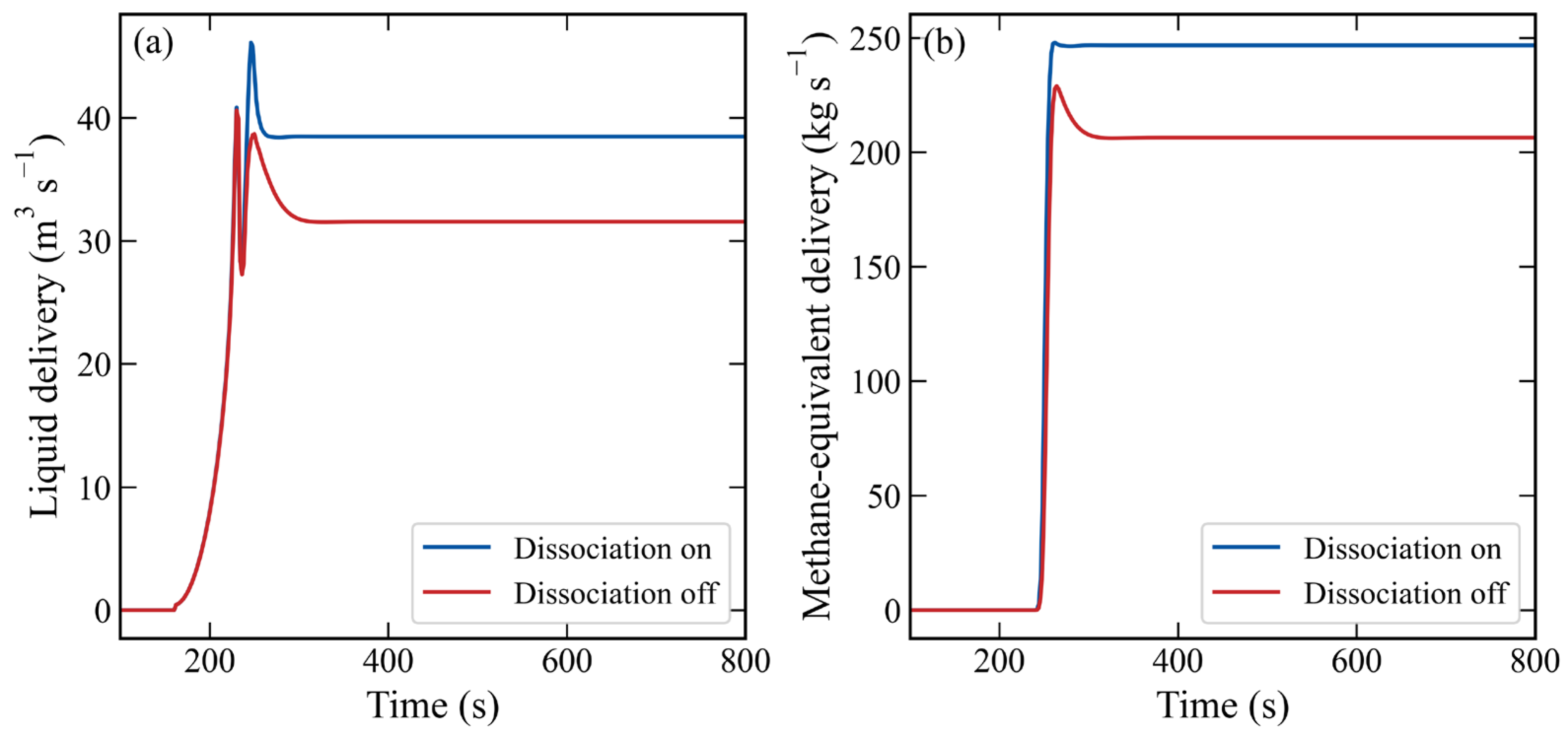
Figure 8 compares the reference calculation with dissociation disabled, keeping geometry, inlet fraction, wall treatment and injected air history unchanged. The nonreactive case delivers approximately 31.6 m3 s−1 of liquid and 1539.1 kg s−1 of solid hydrate. Enabling dissociation raises liquid delivery by approximately 21.9% and methane-equivalent delivery by approximately 19.5% while reducing the outlet solid mass. Specific air use decreases from approximately 6.4 × 10⁻² to 5.4 × 10⁻² Nm3 kg−1 of methane equivalent. These changes describe the modelled contribution of decomposition-generated gas at this operating point.
Figure 8.
Effect of enabling dissociation with unchanged inlet hydrate fraction and external air supply: (a) liquid delivery and (b) methane-equivalent delivery, including both free and hydrate-bound methane.
The methane-equivalent gain accompanies increased intake: the prescribed inlet fraction permits a higher solid feed when liquid transport strengthens. Decomposition redistributes the supplied methane between phases without creating additional methane mass. Both cases retain external air, so this comparison does not establish compressor-free self-lift.
Decomposition-generated methane changes column density, slip and pressure losses, assisting lift. Latent cooling simultaneously reduces the temperature difference driving decomposition. Shrinking particles increase interfacial area per unit remaining solid volume, while residence time also changes. The product split is consequently a coupled hydraulic and thermal response.
The axial source terms identify the active dissociation region. Using a threshold of 0.1% of the maximum local latent sink to identify the active region, its lower edge in the reference case is approximately 303 m below sea level, close to the air port. Within the implemented partial-pressure closure, injection dilutes methane and lowers the equilibrium temperature. The change near the port thus contains a gas composition effect as well as the axial pressure change. The sharp local variation should be interpreted in the context of a cell-averaged injection source and an ideal-mixture equilibrium approximation.
The integrated final latent sink is approximately 346.7 MW, compared with approximately 316.9 kW of wall input, a ratio of about 1.1 × 10³. In Equation (20), liquid advection and sensible cooling therefore dominate the thermal response. These are source magnitudes within the adopted liquid temperature approximation, not a demonstration of total-mixture enthalpy closure. The cooling should not be attributed solely to gas expansion because expansion work is not included.
Doubling the particle heat transfer coefficient increases methane gas delivery from approximately 103.3 to 157.1 kg s−1 and cools the top cell from approximately −1.2 to −1.9 °C, while liquid delivery increases by approximately 4.0%. Insulating the wall gives approximately 38.5 m3 s−1 of liquid and 103.3 kg s−1 of methane, essentially the baseline values. The particle closure is therefore more influential than wall exchange in this case. Its multiplier is a sensitivity parameter, not a validated conversion from HCFC141b experiments to methane hydrate. The cold state also remains subject to the thermodynamic qualifications in Section 4.4.
4.3. Influence of Gas Injection on Transport and Recovery Form
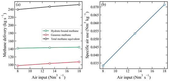
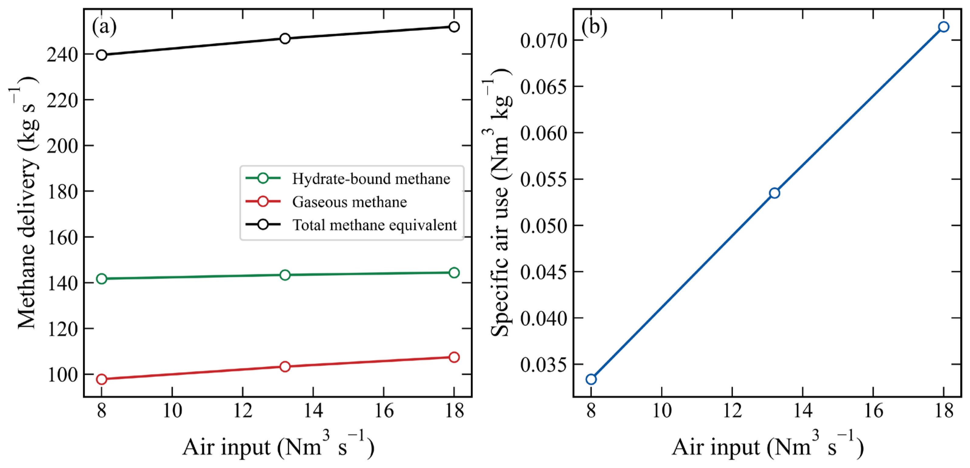
Figure 9 and Table 4 compare air supplies of 8, 13.2 and 18 Nm3 s−1 at a fixed 300 m port, separating free methane, hydrate-bound methane and their sum. Liquid delivery increases from approximately 37.3 to 39.3 m3 s−1. Thus, a 125.0% increase in air supply gives only about a 5.3% throughput gain. Specific air use increases because methane-equivalent output grows much less than the supplied air. Section 4.5 converts the same comparison into an explicitly assumed compressor work estimate.
Figure 9.
Directly simulated (a) gas, hydrate-bound and total methane delivery and (b) specific air use versus normal-volume air supply, with connecting segments used only as guides.
Table 4.
Developed delivery and product split under different injection conditions.
The sampled range shows diminishing transport gains where hydrate-generated gas already assists lift. Holdup, slip and friction prevent a linear input–output extrapolation. Three points do not locate a continuous optimum; an operating target and compressor model are needed for an economic choice.
At fixed 13.2 Nm3 s−1 air supply, moving the port from 150 to 450 m increases predicted liquid delivery from approximately 34.5 to 39.8 m3 s−1. Methane gas output increases from approximately 91.8 to 103.9 kg s−1, and solid output also increases. A deeper port changes the gas-assisted length, pressure and particle residence history; it does not simply convert an unchanged solid feed into more gas. The pressure cost of deeper injection is assessed separately in Section 4.5.
Specific air use decreases with injection depth, but compression pressure increases. These are distinct performance measures [4,25,26]. The compressor screening calculation in Section 4.5 quantifies their opposing effects rather than interpreting lower specific air use as an energy optimum.
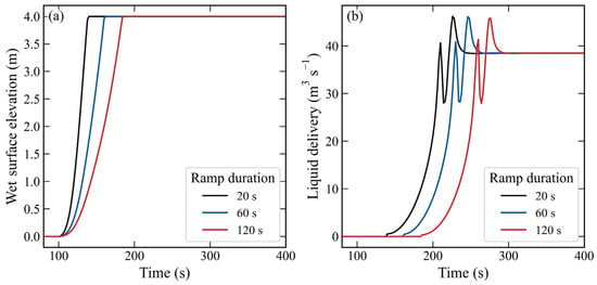
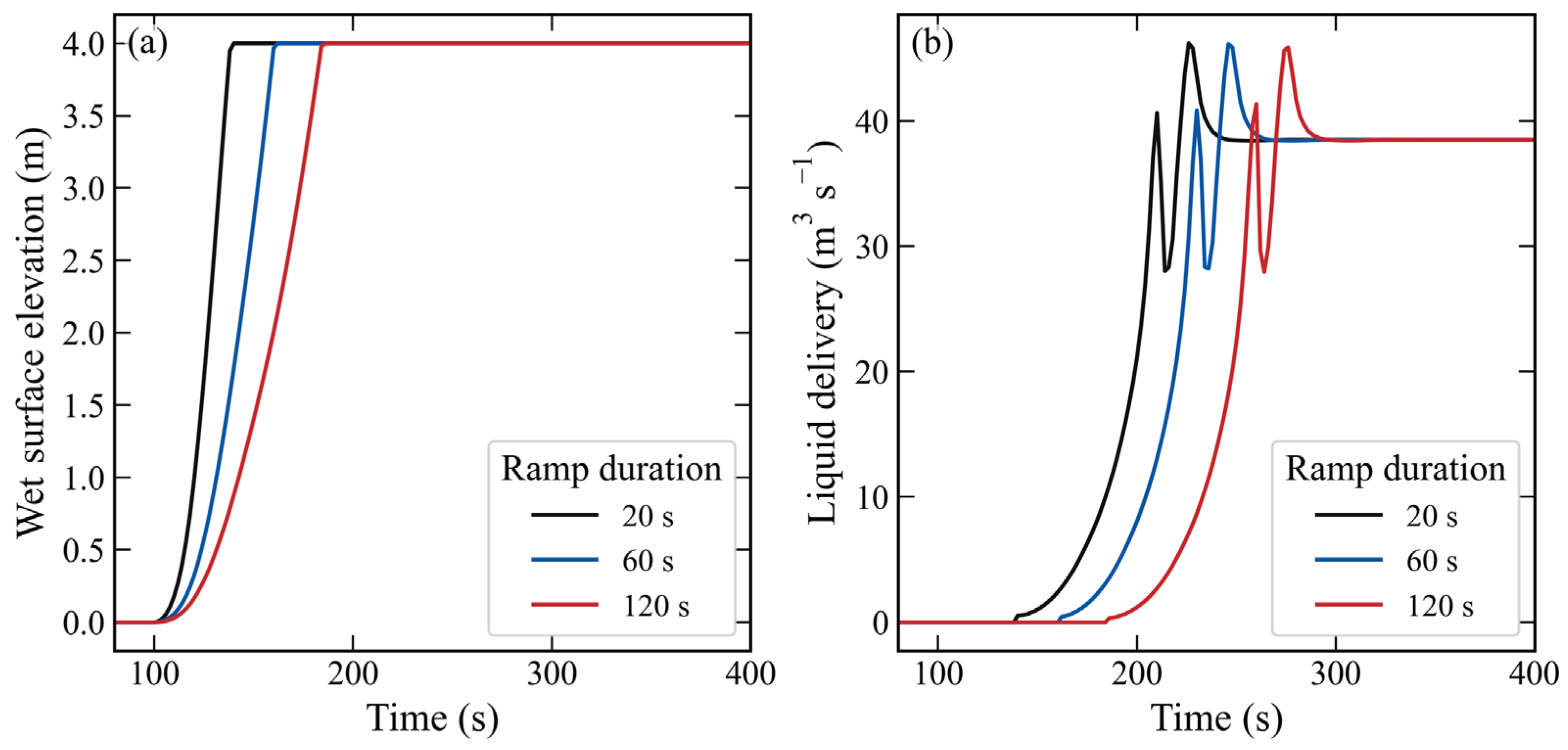
Figure 10 compares 20, 60 and 120 s ramps to the same final air supply. Overflow begins at approximately 138.4, 160.3 and 184.3 s, and liquid settling occurs at approximately 238.0, 258.0 and 286.0 s. Developed deliveries approach the same operating state, while cumulative methane-equivalent products by 800 s are approximately 140.4, 135.5 and 128.5 tonnes. Ramp duration changes startup delay and finite-time product recovery. Because cumulative injected air also differs, these totals alone do not rank compressor energy performance.
Figure 10.
(a) Wet surface elevation and (b) liquid delivery for different air supply ramps starting at 100 s and reaching the same final normal-volume rate.
4.4. Particle Parameters and Intake Depth
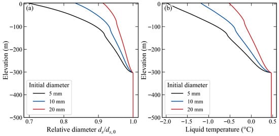
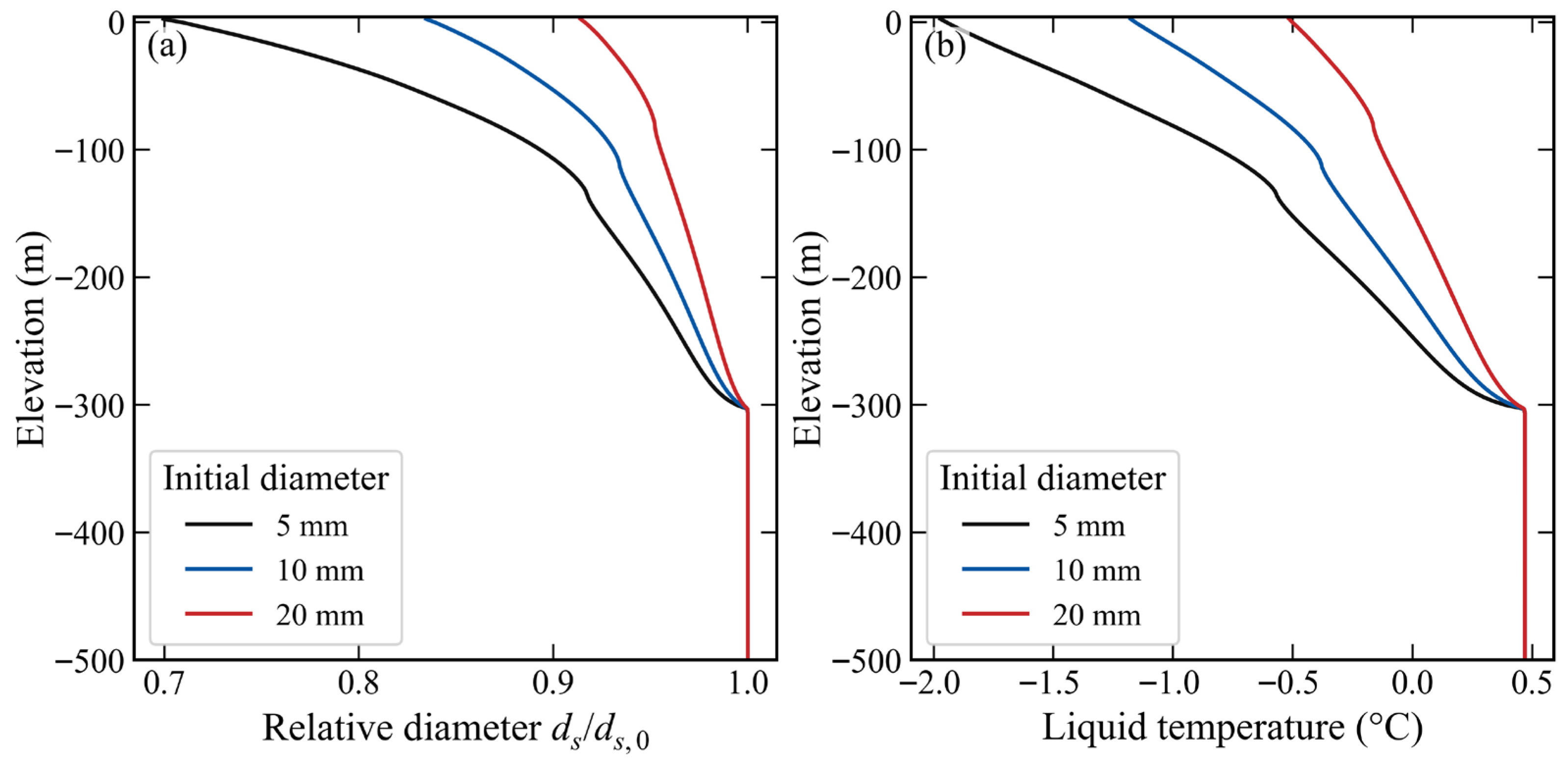
Figure 11 compares 5, 10 and 20 mm particles at the same 5% inlet solid fraction in the original ice-free calculation. Developed solid retention is approximately 34.2%, 58.1% and 76.4%, respectively. Methane gas delivery decreases from approximately 167 kg s−1 for 5 mm particles to 59 kg s−1 for 20 mm particles. Smaller particles provide greater interfacial area per solid volume and undergo greater fractional shrinkage; larger particles retain more hydrate-bound methane.
Figure 11.
Ice-free particle size sensitivity of (a) remaining relative particle diameter and (b) liquid temperature at 800 s with a common inlet solid fraction of 5%.
The corresponding top-cell temperatures are approximately −2.0, −1.2 and −0.5 °C. Stronger decomposition accompanies stronger cooling, which reduces the driving force for further dissociation. Liquid deliveries are 40.3, 38.5 and 38.5 m3 s−1, showing a weaker size dependence than the methane product split. The freezing-limited calculation below quantifies the thermal constraint response of the coldest 5 mm case.
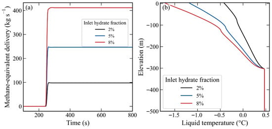
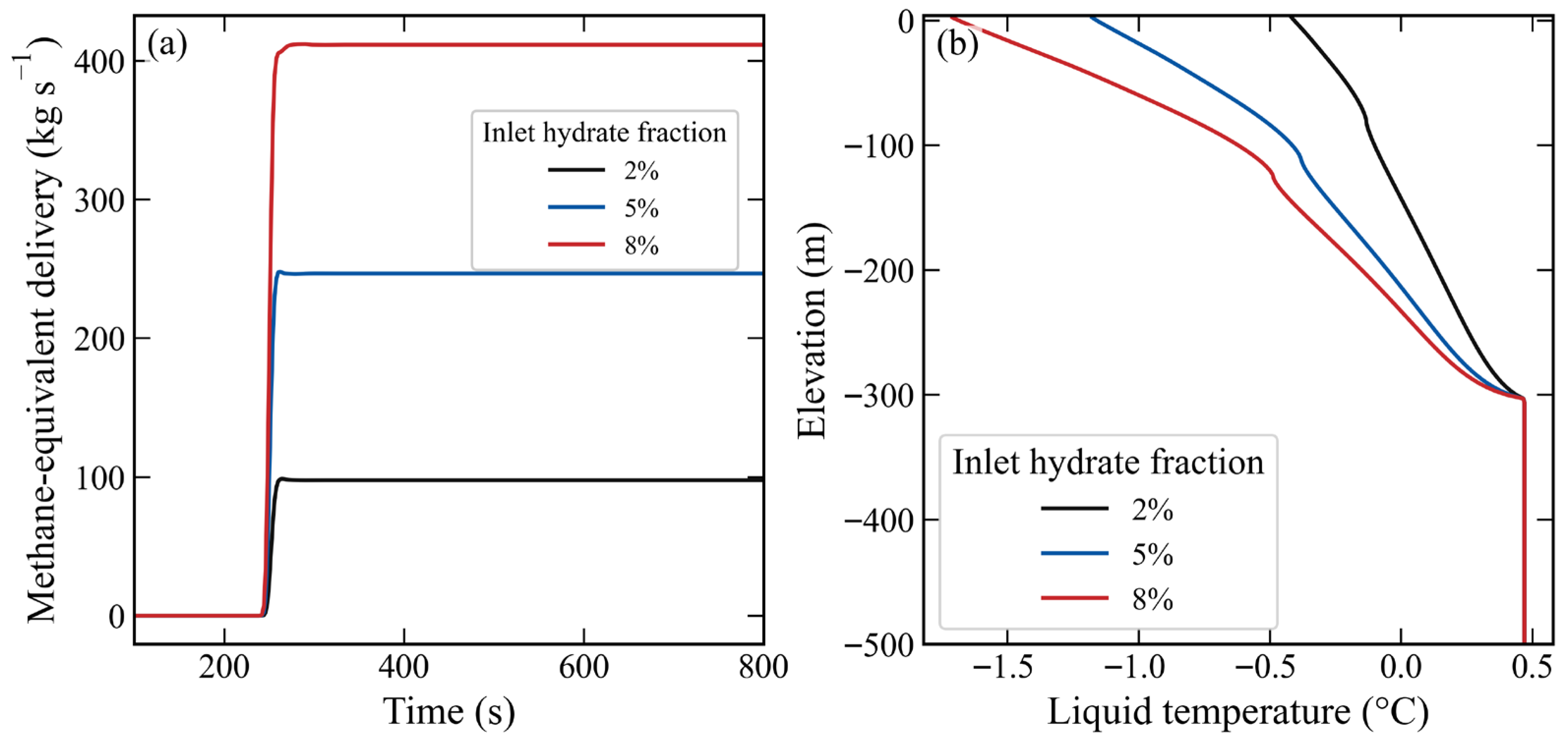
Increasing inlet loading from 2% to 8% increases methane-equivalent delivery from 97.7 to 411.5 kg s−1 (Figure 12), while liquid delivery remains approximately 39.0 m3 s−1 in both cases. The product gain mainly reflects the larger entering hydrate inventory. Solid retention increases from 47.2% to 63.9%, while top-cell temperature decreases from −0.4 to −1.7 °C. Thus, greater total methane input does not require a proportional increase in the fraction recovered as free gas. Table 5 reports the ice-free results; the additional freezing-limited comparison is given at the end of this section.
Figure 12.
Ice-free inlet loading sensitivity of (a) methane-equivalent delivery and (b) final liquid temperature profile at fixed particle diameter and external air supply.
Table 5.
Ice-free particle size and inlet loading predictions at 500 m intake depth.
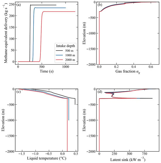
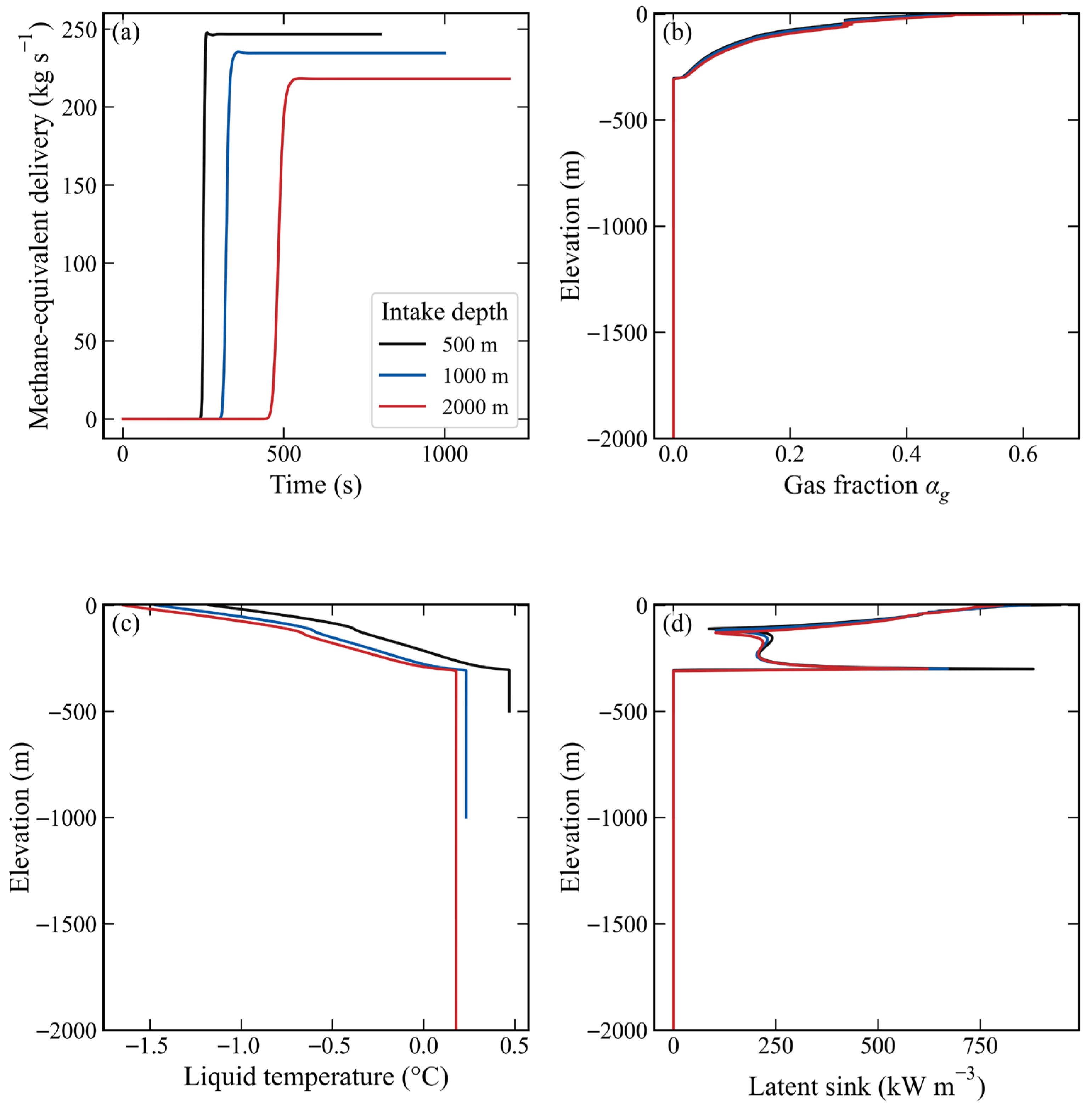
Figure 13 and Table 6 compare intake depths of 500, 1000 and 2000 m, retaining the air port at 300 m, the 2 m diameter and the 13.2 Nm3 s−1 supply. Initial and inlet liquid temperatures are sampled from WOA23 at each intake. These are depth scenarios with their associated cold-water inputs, rather than a strictly isothermal variation of pipe length. The 1000 and 2000 m runs extend to 1000 and 1200 s to include the longer startup.
Figure 13.
Depth scenario (a) methane-equivalent delivery history and final profiles of (b) gas fraction, (c) liquid temperature and (d) latent source density for a fixed 300 m port and WOA23-based intake temperatures.
Table 6.
Depth scenarios with a fixed 300 m air port and 13.2 Nm3 s−1 air supply.
Liquid deliveries at 500, 1000 and 2000 m are approximately 38.5, 36.6 and 34.1 m3 s−1, and methane-equivalent deliveries are approximately 246.7, 234.6 and 218.2 kg s−1. The longer un-injected lower section changes friction, inventory and transit before hydrate enters the strongly gas-assisted region. Significant solid arrival occurs at approximately 246, 310 and 464 s. Methane gas output remains near 103–105 kg s−1, so its share of the methane-equivalent product rises from approximately 41.9% to 48.0%. These scenarios change product form as well as total delivery.
Final top-cell temperatures are approximately −1.2, −1.5 and −1.6 °C. The latent source profiles identify the active upper region; greater deep length is not automatically an equally active dissociation region. These are ice-free predictions for a fixed absolute injection depth. Deepening the port together with the intake would define a different operating series.
The prescribed inlet and initial temperatures at 500, 1000 and 2000 m are reported as 0.5, 0.2 and 0.2 °C, respectively; the WOA23 values are used internally without rounding. Delivery averages use each run’s final 200 s.
The experiments constrain laboratory air–water pumping. Hydrate dissociation, shrinkage, cooling, deep-pipe high-holdup behaviour and the absolute production rates remain model predictions requiring hydrate-specific validation. Salt transport, dissolved methane, reformation, sediment entrainment, fragmentation and an ice inventory are absent. The freezing-limited comparison tests the sensitivity of selected outputs within those limitations and does not replace a multiphase thermodynamic validation.
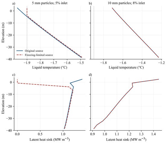
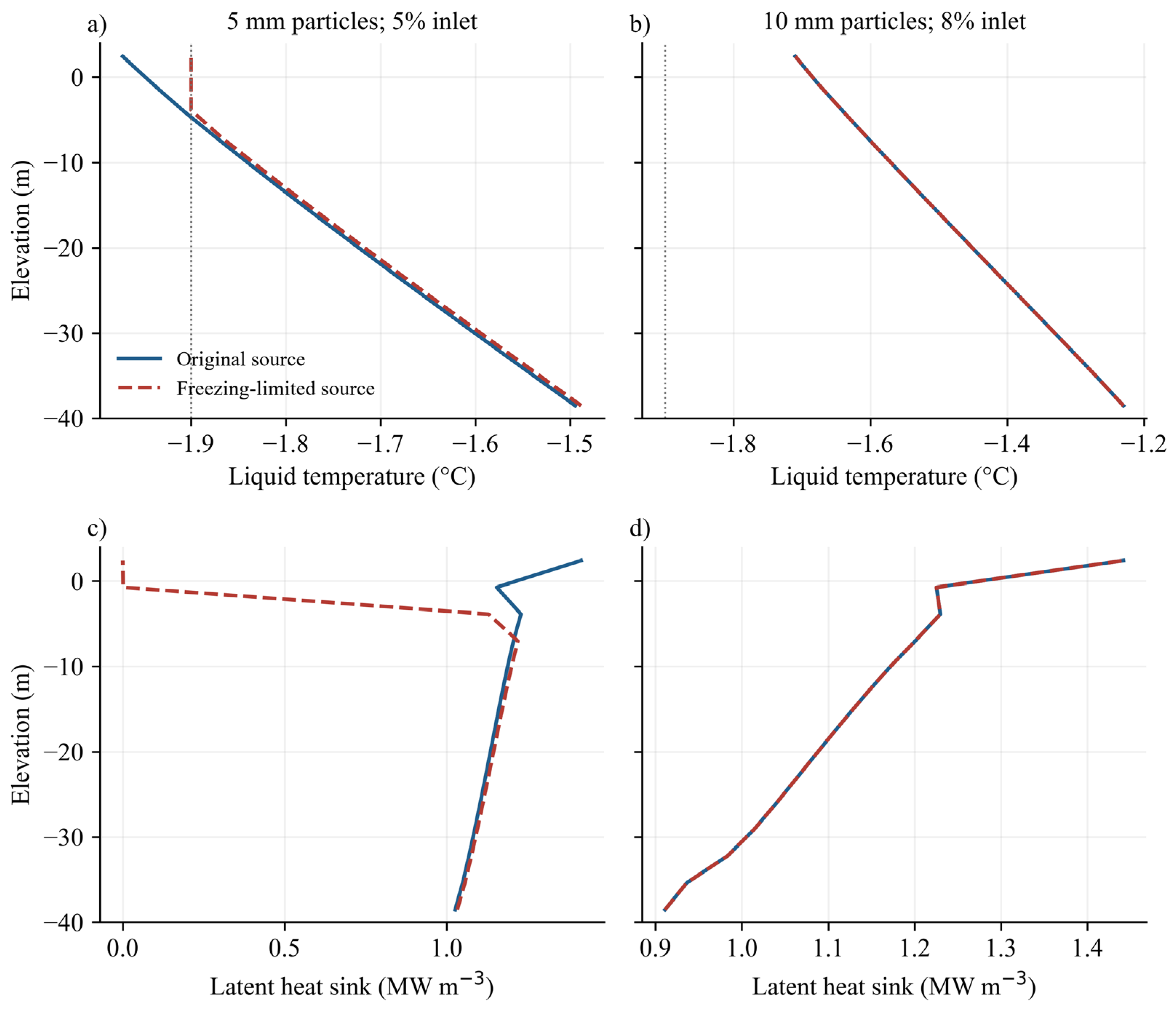
The additional sensitivity applies Equations (22) and (23) to two cold operating cases: 5 mm particles at 5% inlet solid fraction and 10 mm particles at 8% inlet solid fraction. Each constrained case is paired with an original source calculation on 160 cells through 800 s using identical geometry, air injection, thermal boundary and numerical controls. Table 7 gives arithmetic means of the common 2 s outputs over 600–800 s; solid retention is the ratio of the mean solid outlet and inlet mass rates over the same window. Figure 14 resolves the upper pipe from −40 to +4 m elevation, where the threshold affects the coldest case.
Table 7.
Coupled freezing-limited sensitivity at 160 cells with developed averages over 600–800 s and a fixed −1.9 °C threshold.
Figure 14.
Temperature (a,b) and dissociation latent source density (c,d) from −40 to +4 m elevation at 800 s for the original and freezing-limited 5 mm (a,c) and 8% loading (b,d) cases, with grey dotted lines indicating −1.9 °C and overlapping curves for the 8% pair.
For 5 mm particles, the constraint changes developed methane gas delivery from approximately 167.2 to 160.0 kg s−1 (a 4.3% decrease) and solid hydrate delivery from approximately 648.8 to 714.1 kg s−1 (an approximately 10.1% increase). The top-cell temperature changes from approximately −2.0 to −1.9 °C. At 800 s, the cap acts in the upper three cells, whose centres extend from approximately −3.9 to +2.4 m. Liquid delivery changes by approximately 0.5%, comparable to the 0.5% reference-case spatial sensitivity. This small change is not interpreted as a resolved hydraulic gain. The product partition responds more strongly than liquid throughput. For the 8% loading pair, the minimum saved liquid temperature is approximately −1.7 °C, above the prescribed threshold, and the reported developed outputs are unchanged by the constraint. This case demonstrates that a negative Celsius temperature does not by itself activate the selected sea-water-scale bound.
The 8% ice-free top-cell temperature of approximately −1.7 °C is warmer than the nominal −1.9 °C threshold, whereas the 5 mm value of approximately −2.0 °C is colder. Neither comparison determines the true local ice content. Dissociation releases freshwater, salinity and pressure alter the freezing curve [40], and the particle surface can be colder than the bulk liquid. The present constraint does not include ice mass, fusion enthalpy, salt rejection, dissolved methane, reformation or an ice-layer kinetic resistance. These omissions can affect both gas generation and lift: dissolution retains methane outside the free-gas inventory, reformation reverses mass/heat transfer and ice changes latent heat and particle transport. A phase-consistent extension requires coupled salt, ice and enthalpy balances and saline hydrate equilibrium. Table 7 therefore quantifies a defined model sensitivity; it does not validate subzero dissociation or demonstrate absence of interfacial ice.
The 5 mm cases use 5% inlet solid fraction; the 8% cases use 10 mm particles. ‘Capped’ denotes the fixed −1.9 °C source constraint, with all other inputs unchanged. Across the paired cases and the repeated reference run, maximum cumulative mass budget discrepancies normalized by initial liquid mass remain below 3 × 10⁻⁸. The corresponding upper bound on the unscaled discrete temperature row residual is 2 × 10⁻⁷ K. These are solver consistency checks, not experimental accuracy or a total-enthalpy closure test. Temperature minima refer to profiles saved every 2 s.
4.5. Compressor Work Estimate and Engineering Interpretation
To connect specific air use with energy, Table 8 applies the same transparent compressor calculation to the five cases in Table 4. The assumed suction state is p0 = pN = 101325 Pa and Tc = 293.15 K. The reference discharge pressure is pd = p0 + ρsea gHi, with r = pd/p0. This external hydrostatic pressure is an explicit screening assumption, not a recovered internal port pressure or a complete supply line model. The reversible isothermal reference power is
Piso = pN Qa,N (Tc/TN) ln(r).
Table 8.
Compressor screening estimates using the Table 4 operating cases and the stated pressure and equipment assumptions.
For three equal-pressure-ratio stages, perfect intercooling to Tc, ideal gas heat capacity ratio κ = 1.4 and selected stage isentropic efficiency ηs = 0.75, the shaft power estimate is
P3 = [3κ/(κ − 1)] pN Qa,N (Tc/TN) [r(κ − 1)/(3κ) − 1]/ηs.
The specific compressor work is e3 = P3/(3.6 × 106 ṁeq), in kWh kg−1 of methane-equivalent product when P3 is in watts and ṁeq is in kg s−1. It counts methane in both gas and hydrate products, as does Equation (26). These are calculated steady screening values, not measured equipment performance or a complete startup energy integral. Motor losses, line losses, intercooler auxiliaries, excavation, separation and product conditioning are excluded. The isothermal value is a reversible reference at the assumed pressure, not a demonstrated lower bound for a complete plant.
At a 300 m port, increasing air supply from 8 to 18 Nm3 s−1 increases the estimated three-stage power from approximately 4.7 to 10.6 MW and specific work from approximately 5.4 to 11.7 Wh kg−1. With air supply fixed at 13.2 Nm3 s−1, moving the port from 150 to 450 m raises estimated specific work from approximately 7.6 to 9.6 Wh kg−1, despite the lower specific air use. Thus, the sampled throughput gain does not imply an energy improvement under these assumptions. Actual port pressure histories, gas line losses and compressor maps are needed for equipment selection or a plant optimum. The numerical studies [25,26] likewise show the relevance of compression power, but their different pipe and operating scales preclude direct performance matching.
The reference liquid delivery corresponds to a superficial velocity Ql/A ≈ 12.3 m s−1. A single-liquid screening calculation with the adopted smooth-pipe Fanning relation gives Re ≈ 1.7 × 10⁷, fF ≈ 1.2 × 10⁻³ and Δpf = 2fFρl(Ql/A)2L/D ≈ 0.1 MPa over L = 504 m. The external 500 m hydrostatic head is approximately 5.0 MPa. This friction estimate is only an order-of-magnitude reference; actual multiphase losses depend on holdup, slip and the local liquid velocity, which exceeds the superficial velocity. Particle impact and erosion, bends and fittings, wall roughness, structural loading, gas handling and the air–methane hazard require separate engineering assessment. The assumed 2 m diameter and high delivery are therefore a framework-level case, not a feasibility-qualified production design.
5. Conclusions
A transient gas–liquid–hydrate model has been developed from the author’s gas-lift modelling approach incorporating conservative dissociation, particle shrinkage, liquid cooling and separate air/methane accounting. Its principal findings are as follows:
- (1)
- The air–water comparison captures injection depth dependence while retaining a positive shallow injection bias. The 4 m series is used for calibration. Hydrate dissociation, particle shrinkage and cooling are conditional model predictions requiring experimental validation; numerical conservation is not a substitute for that evidence.
- (2)
- Reference-case overflow starts at approximately 160.3 s, before significant methane and hydrate arrival. Developed liquid and methane-equivalent deliveries are approximately 38.5 m3 s−1 and 246.7 kg s−1, with approximately 41.9% of methane in free-gas form. Startup water discharge and hydrate production are distinct events.
- (3)
- Under the adopted closures, dissociation increases liquid delivery by approximately 21.9% and methane-equivalent output by approximately 19.5% relative to the nonreactive case at the same inlet fraction and air supply. The gain accompanies stronger intake: generated gas assists lift, while latent cooling reduces further dissociation.
- (4)
- The selected Japan Sea exterior gives no appreciable delivery change relative to the matched uniform exterior. Wall input is approximately 316.9 kW versus a modelled latent sink of approximately 346.7 MW. This scale comparison is specific to the large-diameter, high-throughput case and is not a total-mixture enthalpy closure.
- (5)
- Increasing air supply from 8 to 18 Nm3 s−1 raises throughput by approximately 5.3% while increasing specific air use and estimated compressor work per unit product. Deeper injection increases throughput and lowers specific air use but increases the screened compressor work per product under the stated hydrostatic pressure and efficiency assumptions. Particle size primarily changes the methane product split. Cold-case comparisons require the freezing qualification in Section 4.4. With a fixed 300 m port, the 2000 m intake gives approximately 218.2 kg s−1 of methane equivalent and delays significant hydrate arrival to approximately 464 s.
The framework supports controlled comparisons of startup, product form, specific air use and compression work. Near-outlet phase fractions remain sensitive to mesh refinement even when delivery rates vary slightly. Hydrate-specific measurements are needed to assess absolute recovery rates and low-temperature kinetics. Engineering application should combine these transport predictions with phase behaviour verification and controlled gas handling.
The freezing-limited 5 mm calculation reduces methane gas output by approximately 4.3% and raises recovered solid hydrate by approximately 10.1%, while the liquid throughput change is comparable to the demonstrated spatial sensitivity. The 8% loading outputs are unchanged at the stated −1.9 °C threshold. These paired calculations quantify the effect of a declared thermal constraint and identify the cold-case product split as assumption-sensitive. A complete ice/salt enthalpy model requires additional phase balances and experimental evidence.
Funding
This research was funded by the Japan Science and Technology Agency, grant number JPMJSP2108.
Data Availability Statement
The data presented in this study are available on request from the corresponding author.
Acknowledgments
Thanks are given for the financial support of the WINGS-QSTEP (Quantum Science and Technology Fellowship Program) project of the University of Tokyo.
Conflicts of Interest
The author declares no conflicts of interest.
Appendix A. Axial Profile Refinement at a Common Physical Time
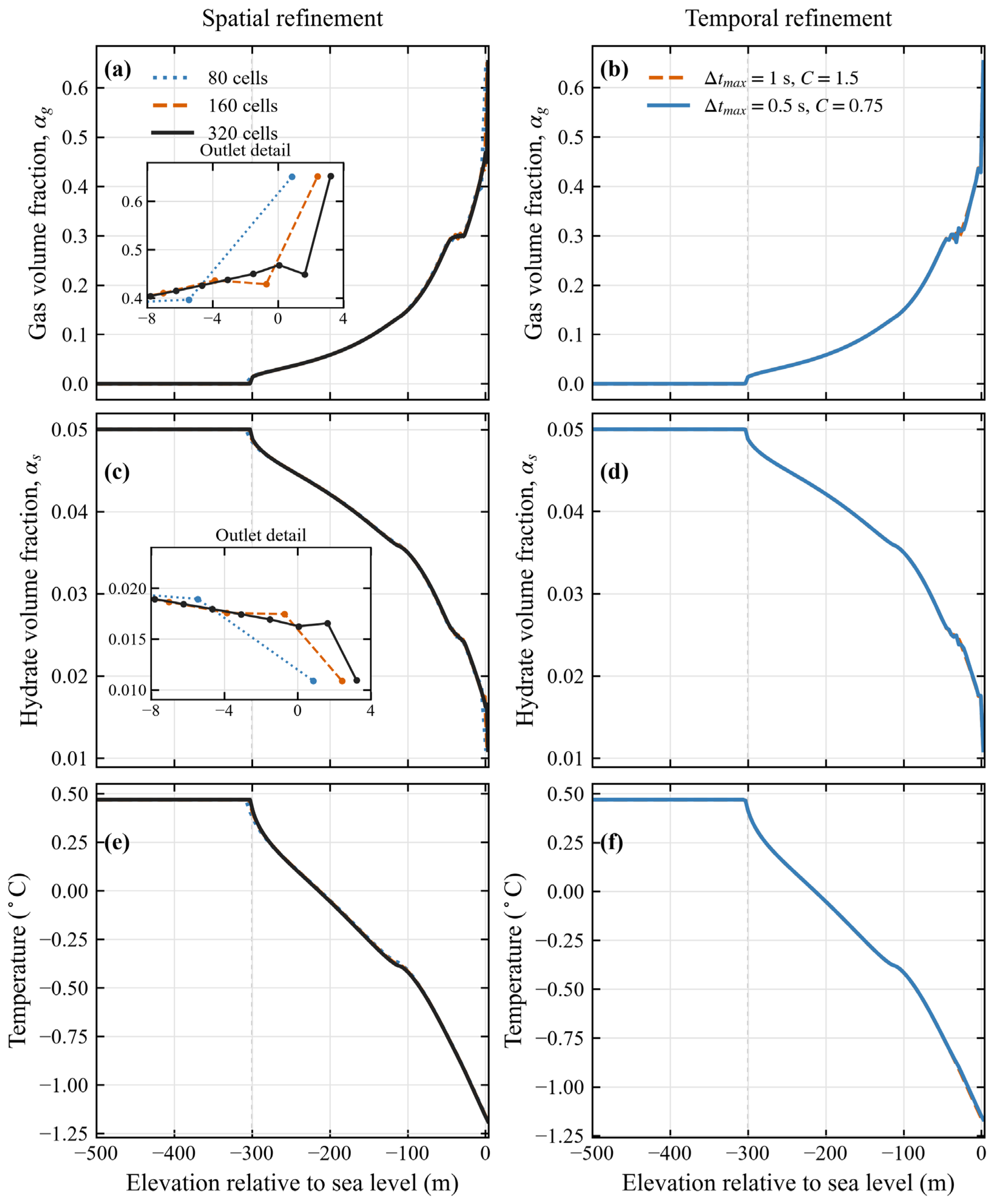
The original 80-, 160- and 320-cell spatial cases and an additional 160-cell temporal control refinement are compared at the common physical time of 300 s, after the wet surface reaches the 4 m outlet. Geometry, composition, closures and boundary histories are identical. The temporal comparison changes the maximum time step from 1 to 0.5 s and the target Courant number from 1.5 to 0.75, retaining the same 0.1 s initial step. Spatial refinement also changes the adaptive Courant-limited time steps; these are coupled numerical sensitivities, not an isolated experimental measurement of spatial convergence order.
For each field, the finer solution is conservatively averaged onto the coarser cells by exact cell overlap integration of its piecewise-constant values. Let δφj be the difference between the coarse value and this restricted reference. The reported L1 discrepancy is Σj|δφj|Δzj/ΣjΔzj and L∞ is maxj|δφj|. Same-grid temporal comparisons require no spatial transfer. Gas and solid discrepancies are absolute volume fraction differences; temperature discrepancies are in kelvin. No percent normalization of absolute kelvin temperatures is used. The profiles include the entire wet column from −500 to +4 m.
Successive spatial refinement approximately halves the domain-mean L1 discrepancies in gas fraction, solid fraction and temperature (Table A1). For 160 versus 320 cells, they are 1.2 × 10⁻³, 4.8 × 10⁻⁵ and 1.4 × 10⁻³ K, respectively. The maximum gas and solid differences remain concentrated in the outlet cell, at approximately 0.1 and 2.9 × 10⁻³. This narrowing feature is not uniformly pointwise converged. The maximum temperature difference is approximately 1.4 × 10⁻² K near the air port. Halving the temporal controls gives L1 discrepancies of 5.0 × 10⁻⁴, 2.1 × 10⁻⁵ and 8.7 × 10⁻⁴ K, with a maximum temperature difference of approximately 1.0 × 10⁻² K. The startup liquid flow peak differs by approximately 5% between 160 and 320 cells and by approximately 2% under temporal refinement, although the 300 s deliveries are less sensitive. Thus, the final delivery, startup peak and local outlet holdup have different numerical sensitivities. The 0–300 s integral of the absolute temporal liquid flow difference is approximately 1.1% of the baseline cumulative delivery, evaluated by trapezoidal integration of common 2 s output samples. These diagnostics support reporting controlled numerical trends with explicit uncertainty; they do not establish a grid-independent outlet peak or validate the physical closures.
Table A1.
Profile discrepancies at 300 s after conservative fine-to-coarse axial averaging.
Norms are absolute volume fraction differences for gas and solid and absolute temperature differences in K. The temporal comparison uses 160 cells with both the maximum time step and target Courant number halved. Figure A1 shows the corresponding unaveraged cell centre profiles.
Figure A1.
Gas fraction (a,b), solid fraction (c,d) and liquid temperature (e,f) at 300 s under spatial (a,c,e) and temporal (b,d,f) refinement with identical physical inputs and common physical coordinates with spatial panel insets resolving the outlet region and markers denoting cell centres.
References
- Boswell, R.; Collett, T.S. Current perspectives on gas hydrate resources. Energy Environ. Sci. 2011, 4, 1206–1215. [Google Scholar] [CrossRef] [Scilit]
- Sloan, E.D., Jr.; Koh, C.A. Clathrate Hydrates of Natural Gases, 3rd ed.; CRC Press: Boca Raton, FL, USA, 2008. [Google Scholar] [CrossRef] [Scilit]
- Ruppel, C.D.; Kessler, J.D. The interaction of climate change and methane hydrates. Rev. Geophys. 2017, 55, 126–168. [Google Scholar] [CrossRef] [Scilit]
- Matsukuma, Y.; Hamaguchi, R.; Minemoto, M. Methane Hydrate Recovery Technology from the Deep Seabed. Jpn. J. Multiph. Flow 2022, 36, 398–406. [Google Scholar] [CrossRef] [Scilit]
- Shimizu, Y.; Hatakeyama, N.; Masuyama, T. Numerical Analysis on Air-Lift Pumping System for Mining Rare-Earth Rich Mud. J. MMIJ 2018, 134, 142–150. [Google Scholar] [CrossRef] [Scilit]
- Pougatch, K.; Salcudean, M. Numerical modelling of deep sea air-lift. Ocean Eng. 2008, 35, 1173–1182. [Google Scholar] [CrossRef] [Scilit]
- Kassab, S.Z.; Kandil, H.A.; Warda, H.A.; Ahmed, W.H. Air-lift pumps characteristics under two-phase flow conditions. Int. J. Heat Fluid Flow 2009, 30, 88–98. [Google Scholar] [CrossRef] [Scilit]
- Hanafizadeh, P.; Ghorbani, B. Review study on airlift pumping systems. Multiph. Sci. Technol. 2012, 24, 323–362. [Google Scholar] [CrossRef] [Scilit]
- Zuber, N.; Findlay, J.A. Average Volumetric Concentration in Two-Phase Flow Systems. J. Heat Transf. 1965, 87, 453–468. [Google Scholar] [CrossRef] [Scilit]
- Ishii, M. One-Dimensional Drift-Flux Model and Constitutive Equations for Relative Motion Between Phases in Various Two-Phase Flow Regimes; Report ANL-77-47; Argonne National Laboratory: Lemont, IL, USA, 1977. [Google Scholar] [CrossRef] [Scilit]
- Hibiki, T.; Ishii, M. One-dimensional drift–flux model for two-phase flow in a large diameter pipe. Int. J. Heat Mass Transf. 2003, 46, 1773–1790. [Google Scholar] [CrossRef] [Scilit]
- Bhagwat, S.M.; Ghajar, A.J. A flow pattern independent drift flux model based void fraction correlation for a wide range of gas–liquid two phase flow. Int. J. Multiph. Flow 2014, 59, 186–205. [Google Scholar] [CrossRef] [Scilit]
- Liu, Y. Development of a wide range numerical model for gas-lift pump system in deep sea mining based on void fraction correlated drift flux model. Ships Offshore Struct. 2025, 1–19. [Google Scholar] [CrossRef] [Scilit]
- Bukhari, S.S.; Abed, R.; Holagh, S.G.; Ahmed, W.H. Flow pattern dependent model for airlift pumps performance: Analytical simulation and experimental verification. Chem. Eng. Res. Des. 2024, 201, 67–81. [Google Scholar] [CrossRef] [Scilit]
- Du, Y.; Zhu, J.; Han, X.; Fu, M.; Li, M.; Shen, Y. Gas state equation and flow mechanism of gas–liquid two-phase flow in airlift pump system. Phys. Fluids 2024, 36, 055142. [Google Scholar] [CrossRef] [Scilit]
- Gray, G.S.; Ormiston, S.J.; Soliman, H.M. Detailed 3D URANS analysis of two-phase flow in an airlift pump. Eur. J. Mech.-B/Fluids 2024, 108, 134–150. [Google Scholar] [CrossRef] [Scilit]
- Kassab, S.Z.; Abdelrazek, A.A.; Lotfy, E.R. Performance and Hydrodynamics of a Bent Riser Airlift Pump. J. Appl. Fluid Mech. 2025, 18, 2453–2464. [Google Scholar] [CrossRef] [Scilit]
- Wang, Y.; Zhang, R.; Liu, Y.; Yin, J.; Yu, L. Flow pattern prediction and structural optimization of variable-diameter air-lift pipelines in deep-sea mining. Ocean Eng. 2026, 362, 126273. [Google Scholar] [CrossRef] [Scilit]
- Li, Y.; Wang, S.; Yang, F.L.; Hu, D.; Lin, P. Numerical investigation of the effect of air injection modes on the hydraulic performance of airlift pump systems. J. Mech. 2026, 42, 193–207. [Google Scholar] [CrossRef]
- Takano, S.; Masanobu, S.; Kanada, S.; Ono, M. Correlation for calculating frictional pressure drops in vertical three-phase flows for subsea-resource production. Ocean Eng. 2023, 275, 114121. [Google Scholar] [CrossRef] [Scilit]
- Takano, S.; Masanobu, S.; Kanada, S.; Ono, M. Experimental studies on velocities of gas- and solid-phases in gas-liquid-solid three-phase flow for subsea resource productions. Multiph. Sci. Technol. 2023, 35, 35–54. [Google Scholar] [CrossRef] [Scilit]
- Höhn, R.L.; Arabi, A.; Ballesta, S.V.V.; Sassi, P.J.; Pallarès, J.; Stiriba, Y. Analysis of flow regimes and volumetric phase fraction of vertical upward gas–liquid–solid three-phase flow. Can. J. Chem. Eng. 2025, 103, 4513–4539. [Google Scholar] [CrossRef] [Scilit]
- Kidaka, Y.; Sugiyama, K. Three-phase flow analysis of rising shallow methane hydrate in gas lift system. Ocean Eng. 2024, 303, 117738. [Google Scholar] [CrossRef] [Scilit]
- Kidaka, Y.; Sugiyama, K. Flow analysis of rising shallow methane hydrate in gas-lift system with a tapered pipe and multiple gas injections. Multiph. Sci. Technol. 2025, 37, 1–19. [Google Scholar] [CrossRef] [Scilit]
- Shimizu, Y.; Sugihara, M. A Numerical Approach to Transporting Shallow-type Methane Hydrate from Deep Sea Using a Gas-lift Pump. J. MMIJ 2025, 141, 115–124. [Google Scholar] [CrossRef] [Scilit]
- Shimizu, Y.; Sugihara, M. Multi-Task Type Vertical Transport System Using Air-Lift Pump for Mineral and Energy Resources in Deep Sea-A Numerical Analysis on the System for Shallow-Type Methane Hydrate-. J. MMIJ 2026, 142, 38–45. [Google Scholar] [CrossRef] [Scilit]
- Kim, H.C.; Bishnoi, P.R.; Heidemann, R.A.; Rizvi, S.S.H. Kinetics of methane hydrate decomposition. Chem. Eng. Sci. 1987, 42, 1645–1653. [Google Scholar] [CrossRef] [Scilit]
- Clarke, M.; Bishnoi, P.R. Determination of the activation energy and intrinsic rate constant of methane gas hydrate decomposition. Can. J. Chem. Eng. 2001, 79, 143–147. [Google Scholar] [CrossRef] [Scilit]
- Zhang, L.; Wu, B.; Li, Q.; Hao, Q.; Zhang, H.; Nie, Y. A fully coupled thermal–hydro–mechanical–chemical model for simulating gas hydrate dissociation. Appl. Math. Model. 2024, 129, 88–111. [Google Scholar] [CrossRef] [Scilit]
- Ranz, W.E.; Marshall, W.R. Evaporation from drops, Parts I and II. Chem. Eng. Prog. 1952, 48, 141–146, 173–180. [Google Scholar]
- Whitaker, S. Forced convection heat transfer correlations for flow in pipes, past flat plates, single cylinders, single spheres, and for flow in packed beds and tube bundles. AIChE J. 1972, 18, 361–371. [Google Scholar] [CrossRef] [Scilit]
- Clift, R.; Grace, J.R.; Weber, M.E. Bubbles, Drops, and Particles; Academic Press: New York, NY, USA, 1978. [Google Scholar]
- Locarnini, R.A.; Mishonov, A.V.; Baranova, O.K.; Reagan, J.R.; Boyer, T.P.; Seidov, D.; Wang, Z.; Garcia, H.E.; Bouchard, C.; Cross, S.L.; et al. World Ocean Atlas 2023, Volume 1: Temperature; Mishonov, A., (Technical Ed.); NOAA Atlas NESDIS 89; National Centers for Environmental Information (NCEI): Asheville, NC, USA, 2024. [Google Scholar] [CrossRef]
- Thomas, P.D.; Lombard, C.K. Geometric Conservation Law and Its Application to Flow Computations on Moving Grids. AIAA J. 1979, 17, 1030–1037. [Google Scholar] [CrossRef] [Scilit]
- Roache, P.J. Perspective: A Method for Uniform Reporting of Grid Refinement Studies. J. Fluids Eng. 1994, 116, 405–413. [Google Scholar] [CrossRef] [Scilit]
- Health and Safety Executive. Prevention of Fire and Explosion, and Emergency Response on Offshore Installations. Approved Code of Practice and Guidance, L65, 3rd ed.; HSE Books: Sudbury, UK, 2016. Available online: https://www.hse.gov.uk/pubns/books/l65.htm (accessed on 15 October 2026).
- Oran, E.S.; Gamezo, V.N.; Zipf, R.K., Jr. Large-Scale Experiments and Absolute Detonability of Methane/Air Mixtures. Combust. Sci. Technol. 2015, 187, 324–341. [Google Scholar] [CrossRef] [Scilit]
- Stern, L.A.; Circone, S.; Kirby, S.H.; Durham, W.B. Anomalous preservation of pure methane hydrate at 1 atm. J. Phys. Chem. B 2001, 105, 1756–1762. [Google Scholar] [CrossRef] [Scilit]
- Zhu, Y.-J.; Chen, Y.-Z.; Xie, Y.; Zhong, J.-R.; Wang, X.-H.; Xiao, P.; Sun, Y.-F.; Sun, C.-Y.; Chen, G.-J. Microscopic experimental study on the effects of NaCl concentration on the self-preservation effect of methane hydrates under 268.15 K. Chin. J. Chem. Eng. 2024, 73, 1–14. [Google Scholar] [CrossRef] [Scilit]
- IOC; SCOR; IAPSO. The International Thermodynamic Equation of Seawater–2010: Calculation and Use of Thermodynamic Properties, Intergovernmental Oceanographic Commission; Manuals and Guides No. 56; UNESCO: Paris, France, 2010; Available online: https://www.teos-10.org/pubs/TEOS-10_Manual.pdf (accessed on 15 October 2026).

Disclaimer/Publisher’s Note: The statements, opinions and data contained in all publications are solely those of the individual author(s) and contributor(s) and not of MDPI and/or the editor(s). MDPI and/or the editor(s) disclaim responsibility for any injury to people or property resulting from any ideas, methods, instructions or products referred to in the content. |
© 2026 by the author. Licensee MDPI, Basel, Switzerland. This article is an open access article distributed under the terms and conditions of the Creative Commons Attribution (CC BY) license.