


Abstract
Shipboard data servers sample many sensor channels at a fixed interval, although many channels repeat their value or vary only within a small tolerance. This study examines how far transmission to shore can be reduced while the received stream remains fit for its intended use. Traces from five liquefied natural gas (LNG) carriers with 1300–1870 channels per vessel were cleaned of no-signal sentinels and profiled by value type and temporal behaviour. Seven policies, from full and compressed transmission to change-only, heartbeat, deadband, spike-aware, and adaptive transmission, were applied and reconstructed at the receiver. Indicators derived from the International Organization for Standardization and International Electrotechnical Commission (ISO/IEC) standards 25012 and 25024 were evaluated against acceptance profiles for alarm monitoring, condition-monitoring dashboards, and aggregate evidence. Applied to all channels, the adaptive policy removed 82.8% of the records, with a normalised error of 0.08% on numeric channels and no missed state transition. Savings ranged from 73.9% on all float channels to 98.7% on quasi-static ones. Gzip reduced bytes by 85.9% but removed no records, and compressing the reduced stream removed a further 51–78% of the compressed bytes. Staleness, rather than reconstruction error, limited the reduction, so heartbeats must be set in elapsed time.
1. Introduction
Maritime digitalisation turns shipboard sensor data into a shore-facing data product used for condition monitoring, energy management, remote diagnosis, operational decision support, and environmental compliance [1,2,3]. The Maritime Single Window (MSW), the International Maritime Organization (IMO) Data Collection System (DCS), the Carbon Intensity Indicator (CII), the European Union (EU) Emissions Trading System (EU ETS), and FuelEU Maritime all raise the value of reliable operational data interfaces between ship and shore [4,5,6,7,8,9,10,11]. The engineering objective is no longer simply to transmit more data. It is to transmit data in a form that remains fit for its intended shore-side use while controlling communication, storage, and processing cost.
An often overlooked property of shipboard sensor data is that repeated acquisition does not necessarily imply repeated information change. A vessel may record hundreds or thousands of channels at a fixed sampling interval, but many channels remain unchanged, change only rarely, or vary only within a small engineering tolerance [12,13]. Alarm flags, equipment statuses, operating modes, counters, setpoints, and some floating-point measurements can be static, quasi-static, event-driven, slowly varying, or monotonic over long periods. Transmitting every sampled value at the acquisition frequency can therefore create a large number of records whose information value is small relative to their communication cost. General-purpose compression can reduce wire bytes after records have been generated, but it does not reduce message generation, queue growth, ingestion burden, or the recovery load created by unnecessary updates [14,15]. Reducing the records themselves is the older industrial tradition of exception reporting and deadband-based historian methods and of more recent event- and self-triggered transmission designs [16,17,18,19,20,21].
This paper frames the problem as a data-quality trade-off rather than as a pure compression problem. The International Organization for Standardization/International Electrotechnical Commission (ISO/IEC) Systems and software Quality Requirements and Evaluation (SQuaRE) series provides a useful basis for this framing because it treats data quality as a set of measurable characteristics rather than as a single notion of correctness [22,23,24]. In this paper, selected SQuaRE-inspired characteristics are mapped to shipboard transmission metrics. Efficiency is represented by byte and message reduction. Accuracy is represented by reconstruction error. Completeness is represented by event miss and spike recall. Currentness is represented by receiver-side staleness. Consistency is represented by the preservation of aggregate and temporal behaviour. This mapping allows change-aware transmission policies to be evaluated not only by how much traffic they save, but also by what kind of data quality they preserve or sacrifice. In this paper, a balance between efficiency and data quality is therefore not a single optimum. It is defined operationally as the policy that transmits the fewest records while satisfying an explicit, service-specific acceptance profile, namely, bounds on reconstruction error, event and excursion preservation, receiver-side staleness, and aggregate error that are stated before the policies are compared (Section 3.7).
This study evaluated change-aware transmission using operational traces from five liquefied natural gas (LNG) carriers sampled on a sub-minute grid. The dataset contains 9.8 million timestamped rows and 1300–1870 sensor channels per vessel after sentinel cleanup. Each channel was first profiled by value type and temporal behaviour, including boolean, enumeration, counter, string, and floating-point channels and static, quasi-static, event-driven, slowly varying, continuously varying, monotonic, and noisy behaviours. We then compared full transmission, compressed full transmission, exact change-only transmission, change transmission with heartbeat, deadband transmission, spike-aware deadband transmission, and a type-and-behaviour adaptive policy. The receiver reconstructed the shore-side time series, and each policy was evaluated using both communication metrics and SQuaRE-inspired data-quality metrics.
The study is organised around three research questions (RQs), each answered by a defined set of indicators and analyses (Table 1).
Table 1.
RQs, indicators, and where they are answered.
- RQ1. How much of a repeatedly sampled shipboard stream is exactly or quasi-constant once no-signal sentinels are removed, and how does this differ by value type, vessel, missing-data level, and operating phase?
- RQ2. Which parts of the transmission cost do compression and change-aware record suppression each remove, when both are measured on the same channel population, record format, and codec?
- RQ3. Which policy transmits the fewest records while staying within an explicit, service-specific data-quality acceptance profile, and how robust is that choice to the deadband, heartbeat, sampling interval, and transport disturbances?
The study builds on established mechanisms, namely, exception reporting, deadbands, heartbeats, and compression, and its contribution is empirical and methodological. It is threefold. First, it provides a cross-vessel profile of value type and temporal behaviour for five shipboard data servers, including the effect of no-signal sentinels, missing data, and operating phase on the apparent stability of the channels. Second, it turns selected ISO/IEC SQuaRE data-quality characteristics into transmission-level indicators and acceptance criteria so that a reduced stream can be accepted or rejected for a stated shore-side service rather than judged by bytes alone. Third, it compares compression, change-only, heartbeat, deadband, spike-aware, and adaptive policies on identical channel populations and identical record formats and reports where each policy meets or fails those criteria.
The remainder of this paper is organised as follows. Section 2 reviews shipboard data standards, SQuaRE data-quality concepts, and related work on time-series compression and change-based telemetry. Section 3 describes the dataset, cleanup, profiling, transmission policies, reconstruction methods, and evaluation metrics. Section 4 presents the cross-vessel results. Section 5 discusses implications and limitations. Section 6 concludes the paper.
2. Background and Related Work
2.1. Maritime Data Standards and Regulatory Reporting
Shipboard sensor data are no longer a local on-board signal. They are an addressable asset in a standardised ship–shore information exchange that is increasingly tied to regulatory reporting and verification. Two complementary layers govern that exchange. The semantic layer is set by ISO 19847, which specifies the requirements for a shipboard data server that collects and shares field data safely and efficiently, and by ISO 19848, which standardises the naming, units, quality codes, and update cycles of sensor channels through a hierarchical data-channel identifier and an accompanying data-channel list [12,13]. These standards make a vessel’s sensor inventory machine-readable, but they do not prescribe a transmission rate or a data-reduction policy for the channels that they catalogue.
The service and regulatory layer is set by IMO and regional frameworks that consume those channels. The MSW institutionalises digital ship–shore information exchange for harbour-clearance and compliance workflows, while the IMO Compendium harmonises message and declaration data across maritime services and has been recently extended to safety-information channels such as Navigational Telex (NAVTEX) [4,5,25]. In the EU, the European Maritime Single Window environment links national single windows and the SafeSeaNet system for electronic port-call data exchange [26]. Environmental and carbon-intensity regimes add operational reporting and aggregate-evidence requirements that depend on shipboard data, including the IMO DCS, the CII, the EU Monitoring, Reporting and Verification regulation, the EU ETS extension to maritime transport, and FuelEU Maritime [6,7,8,9,10,11]. The transport link itself is rarely a uniform pipe as surveys of maritime communication networks emphasise that satellite, aerial, terrestrial, and short-range maritime channels coexist with widely different latency and capacity constraints [27,28]. The downstream services that consume these data range from real-time monitoring and dashboarding to periodic compliance evidence and long-term audit archives, each with different freshness, fidelity, and traceability requirements.
A shipboard sensor stream is typically retained on board in raw archival form, often a columnar file written at the acquisition cadence, while a separate operational stream is transmitted to shore for active monitoring and reporting. The two purposes are different. The raw archive is the system of record and must preserve every recorded value for audit. The operational stream is a derived data product whose granularity should be matched to the downstream service. Conflating the two leads either to over-transmission, in which the operational stream carries every recorded value at the acquisition cadence, or to under-archival, in which the raw record is discarded once a reduced operational view has been sent. This paper assumes that the raw archive is retained on board and focuses on the operational stream.
The standards define what each channel means, and the service and regulatory frameworks define what evidence the shore side must obtain from those channels. Neither layer prescribes whether every sampled value must travel to shore at the acquisition cadence. That decision sits in the shipboard gateway and is an architectural and data-quality problem rather than a standardisation problem.
2.2. ISO/IEC SQuaRE Data Quality Model
The ISO/IEC SQuaRE series provides a structured way to reason about data quality [22]. ISO/IEC 25012 defines a data quality model in which data quality is decomposed into measurable characteristics such as accuracy, completeness, consistency, credibility, currentness, accessibility, compliance, confidentiality, efficiency, precision, traceability, and understandability [23]. The model further distinguishes between inherent quality, which is a property of the data themselves, and system-dependent quality, which depends on the system in which the data are used. ISO/IEC 25024 provides a corresponding set of measurement functions for these characteristics [24]. Although these standards are intended for software and information systems in general rather than for maritime telemetry, the underlying view that data quality is multi-dimensional and measurable applies directly to shipboard sensor transmission.
For change-aware shipboard transmission, the relevant characteristics can be operationalised as communication and reconstruction metrics. Table 2 summarises the mapping used in this paper. Efficiency corresponds to how much of the original byte and message volume is avoided. Accuracy is the closeness between the receiver-side reconstructed series and the original sampled series. Completeness is the preservation of meaningful changes and excursions that the receiving service needs to observe. Currentness is the freshness of the most recent value available at the receiver. Consistency is the preservation of aggregate and temporal behaviour, such as cumulative sums, state transitions, and counter monotonicity, that downstream calculations rely on.
Table 2.
SQuaRE data-quality characteristics mapped to study metrics.
This mapping defines the evaluation lens used here. A transmission policy is not better merely because it sends fewer bytes. It is better when it achieves a favourable balance between efficiency and the data-quality characteristics required by the receiving service.
The indicators are narrower than the corresponding ISO/IEC 25012 definitions, and the difference matters for interpretation. ISO/IEC 25012 describes the quality of data with respect to the real-world entity they represent, partly as an inherent property of the data and partly as a property that depends on the system that stores and delivers them [23]. In this study the reference is not the physical process but the cleaned archived stream recorded on board. Every indicator therefore measures the degradation introduced by transmission, which is a system-dependent property, and none of them certifies the inherent quality of the sensor data. Three characteristics are used in a deliberately restricted sense. Completeness in ISO/IEC 25012 concerns whether required attribute values are present. Here it concerns whether the changes and excursions present in the archive are also present at the receiver, so an event miss is a completeness defect introduced by the policy, while values missing in the archive itself are reported separately as null and sentinel ratios. Currentness in ISO/IEC 25012 concerns whether data are of the right age for the task. Here it is the age of the receiver-side value at the moments when a fresh value exists on board, measured in grid steps and in elapsed seconds. Consistency in ISO/IEC 25012 concerns freedom from contradiction and coherence with other data. Here it is the agreement between aggregates, state sequences, and counter monotonicity computed from the reduced stream and from the archive. ISO/IEC 25024 measurement functions are used as a template for expressing each indicator as a ratio or bounded quantity [24], not as a claim of conformance to the standard.
2.3. Change-Aware Reporting and Time-Series Compression
Reducing the cost of transmitting repeatedly sampled data has a long industrial history. Two related traditions have developed independently. The historian tradition decides which samples are informative enough to retain or report. The time-series compression and columnar storage tradition compresses the samples that have already been generated. The two address different layers of the same cost model and combine cleanly.
The historian tradition is the older of the two. Industrial process historians have long used exception reporting and deadband-like rules to retain only those samples that deviate from the previously reported value by more than an engineering threshold. Vendor implementations such as the AVEVA PI System separate exception reporting at the interface from compression testing at the archive, transmitting only meaningful changes and storing only the points needed to reconstruct the trend within a tolerance [29]. The same logic is formalised at the subscription layer by OPC Unified Architecture (OPC UA), whose DataChangeFilter suppresses value-change notifications within an absolute or percent deadband while preserving status changes [30]. The swinging-door trending algorithm extended this idea to a piecewise-linear envelope that preserves trend slope while discarding intermediate samples [16]. Subsequent work assessed the practical accuracy and downstream impact of process-data compression and showed that the window-size parameter of box-car back-slope compression could be tuned automatically rather than fixed [17,31]. More recent work on statistical deadband reframes the threshold as an event-based reporting rule whose parameter is set from the signal’s own variability, while Zhang et al. propose an adaptive threshold that responds to concept drift to balance reduction rate and reconstruction accuracy in Internet of Things (IoT) settings [18,32]. The common pattern is to suppress non-informative updates at the source, transmit a heartbeat or checkpoint so that the receiver can distinguish silence from steady state, and reconstruct the signal at the receiver by holding the last observation or by interpolating between received points [33].
Heartbeats add a bounded liveness contract so that the receiver can distinguish an unchanged sensor from a silent or disconnected sensor. Spike-aware variants add an exception that forces transmission when the inter-sample step exceeds a larger threshold so that fast excursions are preserved even for wide deadbands. Counter channels can be reduced further by transmitting deltas with periodic checkpoints. On the receiving side, the operational stream is reconstructed for display, alerting, and aggregation purposes by last-observation-carried-forward (LOCF) for state-like channels, by linear or piecewise interpolation for slowly varying floats, and by checkpoint-plus-delta reconstruction for counters.
The compression and columnar-storage tradition operates after records have already been generated. Time-series database systems such as Gorilla apply delta-of-delta encoding on timestamps and exclusive-or (XOR)-based encoding on values to compress monitoring streams in memory [14]. Lightweight integer codecs such as Sprintz target the same problem for IoT-class devices [34]. Recent floating-point codecs such as ACTF further improve the lossless ratio achievable on sensor traces, while dynamic bit-packing exploits per-channel bit-depth variation [35,36]. Bounded-error piecewise-linear approximation generalises this trade-off to multi-fidelity output streams, and evolving multivariate codecs exploit correlation across channels for IoT settings [37,38]. A recent survey of time-series compression catalogues lossless, error-bounded lossy, online, and segment-based variants of these techniques [15]. Columnar transport formats such as Apache Parquet apply column-wise encodings, including run-length, dictionary, delta, and bit-packing, to repeated and similar values within a column. An empirical evaluation of columnar storage formats shows that the achievable compression ratio depends heavily on dictionary encoding, integer decoding, and block compression [39]. The general-purpose codecs used in transport, such as gzip and zstd, exploit byte-level redundancy in serialised payloads. All of these techniques compress the records that the application chooses to emit. They do not decide whether a record should be emitted, and they do not affect message count, queue length, broker fan-out, or per-record processing cost downstream of the compressor. This per-record cost is significant on constrained collectors and a recent survey of the IoT-edge-cloud continuum identifies it as a first-class concern alongside payload size [40,41].
Industrial historian methods and time-series compression therefore reduce different parts of the communication cost rather than the same part. The present study does not propose a new compression algorithm. It evaluates whether simple change-aware reporting policies, in the historian tradition, preserve SQuaRE-inspired data-quality dimensions on multi-vessel shipboard traces while keeping general-purpose compression as a baseline for the byte-size layer.
Table 3 summarises the part of the cost model that each technique addresses and the part it does not.
Table 3.
Cost components reduced by compression and change-aware transmission.
The relevant research question is therefore not whether compression or change-aware transmission is superior in general but how they affect different cost and quality dimensions when applied to repeatedly sampled shipboard sensor streams.
2.4. Literature Review
Recent work has refined the change-aware transmission idea along three lines that are closely related to this paper. The first line is event- and self-triggered control, where the trigger rule itself is designed from observed data rather than from a fixed model. De Persis et al. derive a data-based event-triggered controller and trigger rule for unknown continuous-time linear systems while preserving stability [19]. Liu et al. design a data-driven self-triggered law based on trajectory prediction to reduce communication overhead while maintaining performance [20]. Wang et al. extend the comparison of model-based and data-driven event/self-triggered designs to discrete-time linear systems [42]. These studies focus on closed-loop stability and on the design of the trigger itself rather than on the data-quality implications of the resulting reduced stream.
The second line is prediction- and estimator-driven transmission for sensor networks. Płaczek proposes prediction-based data reduction with dynamic target-node selection for IoT sensor networks, reporting substantial reductions in transmitted samples while preserving downstream selection accuracy [43]. Lee et al. couple an event-triggered transmission rule with twin hybrid filters to reduce sensor traffic while maintaining state-estimation quality in renewable energy resource management systems [44]. Yang et al. propose a semantic-based multi-packet parallel transmission scheme that performs analysis before transmission to mitigate limited-bandwidth constraints [21]. These works share the present paper’s premise that not every sample needs to be transmitted, but they are oriented toward control loops, sensor-network monitoring, or networked control systems rather than toward multi-channel operational shipboard streams evaluated against external data-quality requirements.
The third line is maritime telemetry and analytics, where the demand for shipboard sensor data is treated as given. Liu et al. survey air-to-sea integrated maritime IoT, including enabling technologies and open challenges [2]. Rigas et al. propose an end-to-end deep-learning framework for fault detection in marine machinery based on shipboard sensor time series [3]. Lee et al. extend the IMO Compendium with NAVTEX safety-information messages and demonstrate transport over Message Queuing Telemetry Transport (MQTT) [5]. Downstream anomaly-detection studies on shipboard machinery underscore that preserving rare excursions is operationally important, and recent work on range-aware time-series anomaly metrics shows that point-wise recall undercounts the cost of missed excursion ranges, motivating excursion-recall measures that operate over the surrounding window [45,46]. These studies confirm that shipboard sensor data are increasingly used as an analytics input and as a digital service across ship and shore, but the question of how aggressively the operational stream can be reduced while keeping the downstream service viable has received comparatively little attention.
A small number of maritime studies address telemetry reduction and edge-gateway processing directly. Surveys of the Internet of Ships list satellite communication, maritime data collection, and data management among its open challenges [47], and identify edge computing as the means of meeting the latency and processing requirements of ships close to the data source [48]. Ferreira and Martins propose an edge computing approach for a fishing-vessel-monitoring system that transmits in real time only data indicative of abnormal behaviour and defers the rest to port, reporting communication savings of 70–90% [49]. Michala et al. propose edge processing of machinery vibration for vessel condition monitoring and, using laboratory measurements and an open bearing dataset, report a reduction in the transmitted volume by about three orders of magnitude without changing the decision-support output [50]. Jurdana et al. propose an adaptive shipboard data compression method based on differential binary encoding for remote voyage monitoring of autonomous ships [51], and Zhang and Zeng combine quantisation, predictive coding, and arithmetic coding to fit ship status data into narrow-band BeiDou short messages [52]. These studies demonstrate the value of reducing data on board, but each addresses a single signal class, such as vibration or vessel position, a single encoding, or a bandwidth target. They do not profile the whole multi-type channel inventory of a shipboard data server, do not separate record suppression from byte compression on the same records, and do not state which data-quality properties the reduced stream must retain for a given shore-side use.
Across all three lines, data quality appears to be a dimension that is seldom named explicitly. Transmission reduction is reported in bytes, packets, or trigger rate, while the implications for accuracy, completeness, currentness, and consistency are typically left implicit. Maritime data standards and reporting frameworks (Section 2.1) define what each channel means and what evidence the shore side must obtain, but they do not specify a transmission policy. The SQuaRE data-quality model (Section 2.2) defines a measurable language for those properties but has, to our knowledge, mainly been applied to general information systems rather than to shipboard telemetry. The industrial historian tradition (Section 2.3) suppresses non-informative updates at the source, often on single signals in a single process, rather than on multi-vessel multi-channel shipboard traces and under an explicit data-quality budget. The gap that this paper seeks to address is therefore the combination, namely, an empirical evaluation of change-aware transmission on real shipboard sensor streams for both the maritime-standard semantic layer and the SQuaRE data-quality layer. Relative to the historian and deadband literature, the difference is in the unit of evaluation rather than in the mechanism. Historian studies tune one rule for one signal and judge it by trend fidelity. Here the same small rule set is applied to every channel of five data servers, the rule is selected from a measured profile of each channel, and the outcome is judged against several data-quality characteristics at once, including staleness in elapsed time, excursion preservation over several samples, and robustness to lost and reordered records, which single-signal studies rarely report together.
Table 4 summarises this position. Each row is a research stream rather than a single paper. Y indicates a dimension that the stream treats explicitly, ∼ indicates partial or implicit treatment, and – indicates that it is outside the stream’s usual scope. The column headings abbreviate shipboard data (Ship. data), compression (Comp.), change-aware reporting (Change), data quality (DQ), and receiver-side reconstruction (Recon.).
Table 4.
Position of this paper relative to related research streams.
This paper seeks to address this gap by profiling repeatedly sampled shipboard sensor channels for ISO 19848-style channel semantics, applying full, compressed, change-only, heartbeat, deadband, spike-aware, and adaptive transmission policies, reconstructing the receiver-side stream, and evaluating each policy through SQuaRE-inspired efficiency, accuracy, completeness, currentness, and consistency metrics.
3. Methodology
This study evaluated change-aware transmission policies for repeatedly sampled shipboard sensor data through a controlled trace-replay and reconstruction study, summarised in Figure 1. The workflow had five stages. Per-vessel Parquet traces were loaded, and no-signal sentinels were replaced with nulls. Each channel was then typed and profiled by temporal behaviour. Seven transmission policies were applied to the cleaned traces. The shore-side time series was reconstructed at the receiver. Finally, the reconstructed and original streams were evaluated with SQuaRE-inspired data-quality characteristics and aggregated across the five vessels.
Figure 1.
Five-stage methodology workflow.
The methodology did not involve the design of a new compression algorithm. It tested whether transmission frequency can be decoupled from acquisition frequency while preserving the data quality required by shore-side services. Compression was treated as a baseline, while change-aware transmission was evaluated as a policy that reduces the generation and transmission of redundant records.
3.1. Dataset and Scope
The dataset consists of operational sensor traces collected from five large LNG carriers of similar class, referred to in the remainder of the paper as V1 through V5 to preserve operator confidentiality. Each vessel was stored as a single Parquet file with a sub-minute sampling cadence whose effective median interval differs per vessel. The traces covered approximately 9.8 million timestamped rows in total, with 1300 to 1870 sensor columns per vessel. Four timestamp and metadata columns were excluded from sensor-channel profiling. The remaining channels included navigation, machinery, cargo, fuel, environmental, alarm, status, counter, and mode-related data.
Table 5 summarises the five-vessel dataset. The reported duration is the calendar span between the first and last recorded timestamps for each vessel. The median inter-row interval ranges from 8 s to 60 s across vessels and reflects the per-vessel acquisition system rather than a uniform 15 s grid. All policy and evaluation metrics in this paper were computed in grid steps, with one row per step, so that the comparison across vessels is independent of the absolute time interval. Because the same number of grid steps corresponds to different elapsed times on different vessels, heartbeat intervals and staleness are additionally reported in elapsed time computed from the recorded timestamps of each vessel, and no nominal cadence is assumed. The precise operator identity and collection period are not disclosed under the data-sharing agreement. The LNG carrier traces are used as a high-complexity shipboard sensor workload rather than as a claim that the proposed method applies only to LNG carriers.
Table 5.
Per-vessel dataset summary.
The five vessels share a ship type and an acquisition-system family, but their channel inventories and operating profiles differ. Table 6 gives the functional composition of the channels. V1–V3 carry about 1300 channels each and V4 and V5 about 1870, mainly because of a larger engine-room inventory, and between 234 and 277 channels per vessel are alarm, status, or mode channels according to the catalogue rule. The operating condition is characterised by the Global Positioning System (GPS) speed over ground (SOG). Among the grid steps with a valid speed, the vessels are underway, defined as at least 3 kn, for 56–87% of the time, and the rest covers port stays, anchorage, and manoeuvring. The traces therefore contain both seagoing and stationary operation, and Section 4.1 reports the policy results separately for the two phases. The study does not cover other ship types, other acquisition systems, or sub-second control and vibration data.
Table 6.
Functional composition of the channel inventory and operating profile per vessel.
3.2. Sentinel Cleanup and Numeric Coercion
Removing no-signal sentinel values is a required preprocessing step. The raw export uses values such as -9998 and -9999 to indicate missing samples or communication errors. These are not physical sensor readings. If treated as ordinary values, they create false changes and distort stability metrics such as ZCR and run length. In a representative window of 100,000 rows and 300 columns, sentinel values accounted for approximately 45% of cells, so sentinel cleanup must precede any temporal-behaviour analysis. Over the full traces, the mean sentinel ratio per channel ranges from 0.12 to 0.42 across vessels and the mean null ratio after cleanup from 0.24 to 0.49 (Section 4.1). Because all stability metrics were computed over consecutive valid samples, a high missing-data ratio could in principle make a channel look more stable than it is. Section 4.1 therefore stratifies the policy results by the null ratio.
The cleanup rule replaces a predefined set of string and numeric sentinels with null before type inference, equality checks, or difference calculations. The sentinel set includes -9999, -9998, -9997, -9996, NaN, nan, NULL, null, and empty strings. After cleanup, each column is numerically coerced when at least 95% of its non-null values can be parsed as numeric. This step is necessary because the raw exports store all sensor columns as text, including floating-point values.
3.3. Value-Type Inference and Temporal Profiling
Each cleaned channel is classified by value type and temporal behaviour. Value type describes the form of the recorded values, while temporal behaviour describes how those values evolve over time. The two dimensions need separate treatment. A floating-point channel may be quasi-static, slowly varying, or continuously varying, while an integer channel may be a categorical code or a monotonic counter.
The value-type inference rules are summarised in Table 7. The rules are evaluated in the order listed in the table, and the first rule that matches assigns the type. A column is treated as numeric when at least 95% of its non-null values parse as numbers, and a numeric column is integer-like when every non-null value equals its rounded value. A channel is classified as boolean when it has two or fewer unique non-null values. Numeric integer-like channels with a small number of unique values are treated as enumeration channels, while numeric integer-like channels that are mostly non-decreasing are classified as counters. Remaining numeric channels are classified as floating-point channels. Non-numeric channels with small cardinality are treated as enumeration channels, while other non-numeric channels are classified as string channels. Channels with no usable non-null data after cleanup are marked as empty.
Table 7.
Value-type inference rules.
Because no vendor tag dictionary was available, the inferred types were validated against a semantic label derived from the ISO 19848-style channel path. A channel was labelled state when one of the last path elements named an alarm, trip, fault, warning, shutdown, status, mode, running, open or closed state, a command, or an acknowledgement. It was labelled counter when one of the last elements named run hours, a count, or a total and continuous when one of the last elements named a physical quantity such as temperature, pressure, flow, speed, level, power, current, or position. The labels were checked in that order, and channels without a match remained unlabelled. Table 8 cross-tabulates the semantic label against the inferred type for all 7614 channel instances of the five vessels. Of these, 86.4% receive a semantic label, and the inferred type agrees with the label for 81.6% of the labelled channels. Agreement is 97.7% for state channels and 84.5% for continuous channels.
Table 8.
Validation of value-type inference against path-derived semantic labels for all channel instances.
The disagreements fall into three groups, and their consequence for transmission differs. First, 629 channels named after a physical quantity are interpreted as boolean. Of these, 313 are constant over the whole trace and 308 take only two values in the recorded stream, for example, a generator-engine turbocharger speed or a cylinder combustion pressure that takes only two distinct values over the whole export. These channels receive the lossless change-plus-heartbeat rule of boolean channels, so the misclassification costs some heartbeat traffic but cannot introduce reconstruction error. Second, most channels whose name refers to run hours take only two values in the recorded export and are therefore interpreted as boolean, which again leads to lossless treatment. Conversely, 16 channels with a Mode suffix for a run-hour branch, for example, /Engine/GeneratorEngine1/RunHourGas/Mode, carry several thousand monotonically increasing values and are correctly interpreted as counters even though their last path element suggests a state. Counter and float channels receive the same deadband rule in P6, so confusion between these two types does not change the transmitted stream. Third, 30 of the 1306 state-labelled channels (2.3%) are interpreted as float or counter and would be deadband-coded. For integer state codes, a change of one code unit exceeds the deadband whenever the channel scale is below 100 code units for the 1% threshold, so a transition is still transmitted, but this group is the one in which a metadata-based override is needed. Counters that reset after maintenance or rollover are covered by the monotonicity threshold of 0.95. Of the 129 inferred counters, 116 contain at least one decrease and 29 have a monotonicity score below 0.99, and their reconstruction is evaluated in Section 4.7.
Temporal behaviour was then profiled using the metrics in Table 9. All temporal metrics were computed over consecutive non-null observations rather than over the full timestamp grid. This prevented sensors with sparse but valid reporting from being misclassified as unstable simply because they contain many null grid positions.
Table 9.
Temporal-behaviour profiling metrics.
For floating-point and counter channels, the DSR was computed at five relative thresholds of 0.1%, 0.5%, 1%, 2%, and 5% of an engineering scale. Let denote the cleaned value of channel i at grid step t, and let denote the absolute values of its valid samples. For channel i, the scale is
where and denote the median and the 95th percentile, and the constant prevents division by zero for channels whose cleaned values are all zero or extremely close to zero. The same scale is used for both deadband triggering and NRMSE normalisation, so the reported errors should be interpreted as errors relative to the channel’s observed operational scale rather than relative to a manufacturer-specified physical range. With the valid samples of channel i in time order, the ZCR and the DSR at a relative threshold are
where and applied to a set denotes its number of elements.
3.4. Transmission Policies
Seven transmission policies were evaluated, as shown in Table 10. The policies are designed to separate three mechanisms, namely, full transmission, byte-level compression, and change-aware record suppression. P0 sends every valid non-null sample and serves as the full-transmission baseline. P1 applies gzip compression to the same records as P0, thereby isolating byte-level compression from record reduction. P2 sends only exact changes. P3 adds heartbeat messages to change-only transmission to bound receiver-side staleness. P4 sends floating-point and counter values only when a deadband threshold is exceeded or when a heartbeat interval elapses. P5 adds a spike exception to the deadband policy. P6 applies different policies according to value type and temporal behaviour. Pseudocode for all policies, including the initialisation of the policy state, is given in Appendix B.
Table 10.
Evaluated transmission policies.
For P3, the heartbeat interval is set to 60 grid steps for boolean and enumeration channels and to 240 grid steps for numeric channels. Heartbeats are counted in grid steps, so their elapsed duration depends on the vessel’s sampling interval. With the median intervals of Table 5, the 60-step heartbeat corresponds to 8, 15, 12, 49, and 60 min, and the 240-step heartbeat to 0.53, 1.0, 0.8, 3.3, and 4.0 h for V1–V5. All currentness results are therefore reported in elapsed time per vessel as well as in grid steps (Section 4.6). For P4, the deadband thresholds are 0.1%, 0.5%, 1%, 2%, and 5% of the channel scale, applied with the 240-step numeric heartbeat. For P6, boolean and enumeration channels use change plus the 60-step heartbeat. Floating-point and counter channels are assigned deadband thresholds according to their ZCR, with the 240-step heartbeat. High-ZCR channels with ZCR above 0.9 receive a 1% deadband, medium-ZCR channels with 0.5 < ZCR ≤ 0.9 receive 0.5%, and low-ZCR channels with ZCR ≤ 0.5 receive 0.1%.
Formally, let be the last value of channel i transmitted before step t, and let be the step at which it was transmitted. With a deadband fraction and a heartbeat interval h in grid steps, P4 transmits a valid sample when
P2 and P3 are the special cases without and with a heartbeat, and P5 additionally transmits when , where is the previous valid step and is the spike fraction. For boolean and enumeration channels the deadband condition becomes . The first valid sample of every channel is always transmitted.
P5 sends a sample when the deadband or heartbeat condition of P4 is met, or when the step from the previous valid sample exceeds a spike threshold , here 5% of scale. Whether the spike exception adds anything depends on the base deadband. After every valid sample, a deadband policy with LOCF reconstruction keeps the receiver value within of that sample because otherwise the sample would have been sent. A step larger than therefore moves the new sample at least away from the receiver value, and whenever the deadband condition already fires. The spike exception can only add transmissions when . P5 was therefore evaluated with base deadbands of 0.5% and 2%, below this bound, and 5%, above it, where the spike exception becomes operative.
The deadband ladder spans two orders of magnitude so that the threshold can be selected from the resulting curve (Section 4.4) rather than fixed in advance. The lower end is set by the export resolution of the data. The smallest non-zero step of a float channel is 0.10% of its scale at the median and 0.22% at the upper quartile, so a 0.1% deadband is close to the quantisation step and suppresses mainly repeated or last-digit changes. The upper end, 5%, equals the spike threshold and is where step recall starts to fall. On V1, for a main-engine exhaust-gas temperature, whose recorded resolution is 0.28% of scale, deadbands of 0.5% and 1% correspond to about two and four resolution steps, and for the SOG, whose resolution is 0.56% of scale, to about one and two steps. The P6 assignment uses the wider 1% deadband only where ZCR exceeds 0.9, that is, where the channel repeats its value in more than 90% of consecutive samples and the deadband rarely truncates genuine variation, and uses the tightest 0.1% threshold for low-ZCR channels, where a wide deadband would produce the largest reconstruction error. For a specific deployment the thresholds can be replaced by the measurement uncertainty or alarm hysteresis of each instrument when that information is available from ISO 19848 data-channel properties or vendor documentation.
P6 does not optimise thresholds per channel. It applies a simple reproducible rule that selects the transmission policy from the channel’s measured value type and temporal behaviour, which keeps the policy lightweight enough for a shipboard gateway.
3.5. Receiver-Side Reconstruction
For each policy, the receiver reconstructs the full per-vessel sampling grid from the transmitted samples. The default reconstruction method is LOCF. After the receiver obtains a value, it holds that value until the next value for the same channel is received. LOCF matches the semantics of many operational monitoring systems, in which the latest received sensor value is the current state until updated.
For boolean and enumeration channels, LOCF preserves state semantics when all transitions are transmitted. For counters, reconstruction was evaluated against the transmitted checkpoints or changes. For continuously varying floating-point channels, LOCF is used for three reasons. First, it is causal. The receiver can display a held value as soon as a record arrives, whereas linear interpolation (LERP) between two received samples cannot be computed until the next sample arrives, which for a heartbeat-bounded deadband can be up to one heartbeat interval later. Second, it inherits a hard error bound from the deadband. At every valid step the LOCF value differs from the recorded value by at most , except at steps between a dropped or delayed record and its successor, while interpolation has no such bound across a step change. Third, it is the receiver behaviour assumed by OPC UA data-change subscriptions and by historian exception reporting [29,30]. LERP was evaluated as an alternative in Appendix A, and representative reconstructed series are shown in Section 4.3.
3.6. Evaluation Metrics
The policies were evaluated using communication metrics and SQuaRE-inspired data-quality metrics. Communication metrics quantify the reduction in transmitted records and bytes. Data-quality metrics quantify how well the receiver-side reconstructed stream preserves the original sampled stream.
Let be the original cleaned value of channel i at grid step , let be the receiver-side reconstructed value under a given policy, let be the set of grid steps at which channel i has a valid non-null sample after sentinel cleanup, and let be the set of steps at which the policy transmits a record. Each transmitted record is charged bytes in the logical accounting model. Let be the recorded timestamp of grid step t in seconds. For a set, denotes its number of elements and ∖ the set difference, and denotes the P95 over the valid steps. Table 11 summarises the notation.
Communication metrics. The send ratio, byte rate, and bytes saved for channel i are
The send ratio uses the full timestamp-by-channel grid as the denominator so that null or no-signal positions are not double-counted as transmitted samples, while bytes saved is referenced to the P0 logical baseline that transmits every valid sample. Because every record is charged the same 24 B, logical bytes saved and record reduction are the same quantity for P0 and P2–P6. They differ only for compressed streams. Three levels of cost are therefore kept apart in the results. Logical record reduction counts records and is what a broker, queue, or ingestion service handles. Compressed payload size is measured by serialising the records of each policy into the same text format and passing them through the same codec (Section 4.5). Network overhead, such as per-message headers, topic strings, and Transport Layer Security (TLS) records, is not measured and is discussed qualitatively. The results are reported per channel and then averaged within each vessel, which is the convention of all tables unless stated otherwise. For the whole-stream comparison (Section 4.2), the records of all channels of a vessel are pooled, , so that channels with many valid samples carry proportionally more weight. The 24-byte record model is a logical record-accounting baseline used to compare policies under identical assumptions and should not be interpreted as a packet-level wire-size estimate. Real transport will add per-message protocol headers, topic strings or identifiers, batching framing, and TLS overhead, all of which shift absolute byte counts but not the relative ordering of policies that differ in record count.
Accuracy. Accuracy is measured by RMSE, NRMSE, and the P95 absolute error between the original and reconstructed streams. For channel i, with the engineering scale from Equation (1), these are
RMSE and P95 error are also reported in the recorded engineering unit for representative channels (Section 4.3).
Completeness. For boolean and enumeration channels, let be the set of state-transition steps. The event miss ratio is the fraction of those transitions whose grid step was not transmitted,
For numeric channels, the step recall at threshold , a step size expressed as a fraction of , is defined per channel i as
The spike recall used below is . Because a 5% step exceeds every deadband below 2.5% by the argument of Section 3.4, its value is one by construction for those deadbands, so the step recall is also reported at and , which are comparable to or smaller than the evaluated deadbands. To cover gradual excursions that build up over several samples, the windowed excursion recall counts every step t with and treats it as detected if the receiver series shows a change of the same size, , for some step u within the W steps that follow t, that is, ,
with and grid steps. A receiver-side monitor that applies the same rate-of-change threshold over the same window would therefore raise the same alert within W steps. Events shorter than the sampling interval are not represented in the recorded stream and cannot be evaluated from it. Completeness for lost and reordered records was evaluated separately (Section 4.8).
Currentness. Currentness is the age of the receiver-side value at the moments when a fresh value exists on board. At every valid step , the age is measured both in grid steps and in elapsed time from the recorded timestamps,
and analogously for the elapsed-time age. For P0 the age is zero at every valid step, so the reported values are the staleness added by the policy.
Consistency. Aggregate mean relative error between the reconstructed and original streams serves as a proxy for preserving fuel- and energy-aggregate evidence,
where and are the means of and over . The cumulative-sum error normalised by , is algebraically identical to and is therefore not reported separately. Hourly aggregates of compliance-relevant channels and counter monotonicity are evaluated in Section 4.7.
Transport perturbations. The P6 record stream, and for reference the P0 stream, is replayed under two disturbance conditions. In the first, 1% of records are dropped independently at random. In the second, every record is delayed by an integer number of grid steps drawn uniformly from 0 to 8, so records can arrive out of order within an eight-step window. The receiver either applies records in arrival order, which is plain LOCF, or keeps a per-channel sequence number, here the source step, and discards any record older than the one already applied. The same random draws are used for all channels and policies of a vessel. Table 12 summarises the metrics by data-quality characteristic.
Table 12.
Evaluation metrics by SQuaRE characteristic.
3.7. Data-Quality Acceptance Profiles
To make the efficiency–quality balance explicit, three acceptance profiles are defined for typical shore-side services (Table 13). The thresholds follow common engineering practice, namely, an error well inside the deadband ladder, no lost state transitions, an alert-preserving excursion recall, and staleness of the order of the heartbeat. A policy is accepted for a service on a vessel when at least 95% of the relevant channels satisfy every criterion of the profile. The preferred policy for that service is the accepted policy with the fewest transmitted records. Other thresholds can be substituted for a given service, and the same procedure then selects the operating point.
Table 13.
Data-quality acceptance profiles used to select an operating point.
3.8. Cross-Vessel Aggregation
All policy metrics were first computed per channel and then aggregated within each vessel. Cross-vessel results are reported as the mean and standard deviation over the five vessel-level aggregates. This aggregation strategy prevents vessels with more rows or more channels from dominating the overall result.
Two predefined go criteria were used to determine whether the dataset contains enough quasi-constant behaviour to justify change-aware transmission analysis. First, at least 40% of channels in each vessel should have a ZCR above 0.9. Second, at least 30% of floating-point channels should have a 0.5% DSR above 0.9. These thresholds are not used to tune policies. They are used only to confirm that repeatedly sampled but slowly changing data are sufficiently common across vessels.
Sensitivity analysis was conducted for the deadband threshold by evaluating 0.1%, 0.5%, 1%, 2%, and 5% thresholds. The purpose is to avoid presenting a single arbitrary threshold as universally optimal. Instead, this paper reports the trade-off curve between traffic reduction, reconstruction error, and spike recall. In addition, the heartbeat interval is swept over 4, 20, 60, and 240 steps for boolean and enumeration channels and over 20, 60, 240, and 960 steps for P6 on numeric channels. The results are split by operating phase, using GPS SOG of at least 3 kn as underway and below 3 kn as not underway, and by the null ratio of each channel.
3.9. Implementation
The analysis pipeline was implemented in Python using Polars for columnar data loading and processing, with Numba used for state-propagating loops such as policy simulation and reconstruction. Each vessel was processed in column batches to control memory usage. The profiling stage produces one row per channel, while the policy stage produces one result row per channel-policy combination. All analyses were run on a desktop computer with an AMD Ryzen 7 9800X3D eight-core processor, 32 GB of DDR5-5600 memory, and Windows 11 Education version 10.0.26200, using Python 3.10.6, Polars 1.41.0, Numba 0.65.1, NumPy 2.2.5, zstandard 0.25.0, and the gzip module of the Python standard library. Each vessel was processed as in-memory column batches of 100 to 200 channels read from the Parquet file. The policies were evaluated offline on the stored traces, while the gateway benchmark of Section 4.9 evaluated P6 step by step as a streaming gateway would. The random draws of the stratified samples and of the perturbation experiments used the fixed seeds 20260525 and 20261016. Pseudocode of the policies is given in Appendix B, and pseudocode of the cleanup, profiling, reconstruction, metrics, and perturbation procedures in Appendix C.
All vessels were processed through the same sequence of sentinel cleanup, type inference, temporal profiling, policy simulation, reconstruction, metric calculation, and vessel-level aggregation. Cross-vessel differences therefore reflect the data rather than the implementation.
4. Results
Table 14 summarises the main findings, and the following subsections develop each row. Unless a subset is named, every value refers to the whole channel population to which a policy applies, and values are per-channel means within a vessel averaged over the five vessels and reported as the mean and standard deviation.
Table 14.
Headline results of the evaluation.
4.1. Channel Inventory and Temporal Stability
Table 15 reports the per-vessel value-type inventory and the two go-criterion metrics after sentinel cleanup, and Figure 2 compares the latter with the go criteria. Float DSR is at 0.5% of engineering scale. The four timestamp and metadata columns are excluded from the totals.
Table 15.
Per-vessel value-type inventory and stability after sentinel cleanup.
Figure 2.
Per-vessel stability profile against the two go criteria.
All five vessels pass both predefined criteria. The ZCR > 0.9 fraction is in the 42–60% range, well above the 40% threshold. The float DSR(0.5%) > 0.9 fraction is in the 49–78% range, well above the 30% threshold. Boolean channels are 99.6–100% stable and enumeration channels are 90.9–100% stable in every vessel after sentinel cleanup. The recorded shipboard stream is therefore dominated by exact repeats, quasi-static signals, and slowly varying floats whose update value does not differ meaningfully from the previously sent value.
The number of float channels differs across vessels from 663 to 1192. The two vessels with the largest channel inventories, V4 and V5, have the lowest stability rates, while V2, with the smallest float inventory, has the highest. The variation does not invalidate the framing. Even the lowest-stability vessel V4, at 49.2% float DSR(0.5%) above 0.9, is well above the threshold.
Table 16 reports the per-vessel null and sentinel diagnostics as dimensionless fractions in , giving the mean and P95 across channels. Because ZCR and DSR were computed over consecutive non-null observations (Section 3.3), a channel with a high null ratio may appear stable simply because it reports infrequently. The diagnostics show that null and sentinel ratios vary across vessels but are below 50% on average for every vessel. Stability conclusions in the next subsections should therefore be read together with the channel’s reporting sparsity rather than as claims about the underlying physical process.
Table 16.
Per-vessel null and sentinel ratios.
Table 17 tests whether the missing-data level drives the stability or the policy results. Float channels are grouped by their null ratio after sentinel cleanup. Most channels fall in the 25–50% stratum because on several vessels most channels are written only on part of the grid rows. Across the strata, the P6 bytes saved range from 69.7 to 76.4% without a monotonic trend, and the P6 NRMSE stays between 0.0005 and 0.0009, decreasing slightly as the null ratio increases. The rank correlation between the null ratio and P6 bytes saved is −0.05, and between the null ratio and P6 NRMSE −0.02. The fraction of channels with ZCR above 0.9 is highest in the least-missing stratum, which indicates that missing data do not make channels look artificially stable in this dataset. The extreme strata contain few channels and are reported for completeness rather than as stable estimates.
Table 17.
Float-channel stability and policy results by null-ratio stratum over all vessels.
Table 18 splits the float-channel results by operating phase. Both P4 and P6 save more records when the vessel is not underway because machinery and navigation channels are more often idle in port or at anchor, but the reconstruction error is almost unchanged between the phases. The policies therefore do not trade accuracy for savings when operating conditions change. They only send more records when the signals are more active, which is the intended behaviour of a change-aware rule.
Table 18.
Float-channel results by operating phase averaged over the five vessels.
4.2. Cross-Vessel Policy Comparison
Table 19 reports the cross-vessel policy comparison. Each row is the mean and standard deviation across the five vessels of the per-vessel mean of that metric, and n is the number of channel instances. The send ratio is the fraction of grid positions the policy transmits. Bytes saved is one minus the policy’s transmitted bytes divided by the P0 logical-record baseline at 24 B per record. Event miss is defined only for boolean and enumeration channels, while spike recall, the step recall at 5%, is defined only for numeric channels. The send ratio, event miss, and spike recall are dimensionless fractions in , and NRMSE is reported relative to the engineering scale defined in Equation (1). P6 is reported for all numeric channels to which it applies, together with the row of its 1% sub-rule, which covers the high-ZCR float channels. Figure 3 shows the bytes saved with the standard deviation over the vessels, and its light bar is P6 restricted to the high-ZCR float channels.
Table 19.
Mean and standard deviation of the policy metrics across the five vessels.
Figure 3.
Cross-vessel bytes saved by policy.
P1 gzip in Table 19 and Table 20 compresses a per-channel JSON array of all valid records and is compared with the 24-byte logical record count of P0. Its bytes saved therefore combines a change of format with compression, and Section 4.5 compares all policies with the same format and codec.
Table 20.
Comparison of policies on identical channel populations.
The two P3 rows should not be read as the same policy applied to the same channels. The 60-step heartbeat row applies only to boolean and enumeration channels, where the heartbeat is short and the underlying change rate is low. The 240-step heartbeat row applies only to numeric channels, where the longer heartbeat dominates the send pattern for stable signals. The different send ratios therefore reflect both heartbeat interval and channel-type composition, not a single policy evaluated using two settings.
Table 20 answers the question of which reduction applies to which population on one consistent baseline. For each population, every policy was evaluated on the same channels, and bytes saved are given both as the per-channel mean and pooled over all records of the vessel. On all channels of a vessel, P6 removes 82.8% of the records, P2 70.7%, and P1 gzip none, while P1 reduces the byte volume by 85.9%. On all float channels, P6 saves 73.9% of the bytes at an NRMSE of 0.0008, which is less than P4 at a uniform 0.5% or 1% deadband, which save 84.6% and 89.1%, but at a lower error. Savings close to 99% are confined to the high-ZCR float channels, which make up 17% of the float channel instances.
The five-vessel standard deviation of bytes saved is at most 6.1 percentage points across the reduction policies, and the relative ordering of policies is the same on every vessel.
4.3. Results by Value Type
Table 21 reports the per-value-type aggregates. Each policy row aggregates across vessels using rows = channels_per_vessel × vessels. For boolean and enumeration channels we report event miss, and for numeric channels we report NRMSE and spike recall. NRMSE is expressed relative to the engineering scale, and event miss and spike recall are fractions in .
Table 21.
Per value-type policy results, cross-vessel aggregate.
For boolean and enumeration channels, change-only transmission is lossless and saves 99.9% and 99.2% of the records, and a 60-step heartbeat costs 2.4 percentage points of that saving in exchange for bounded staleness. For counter channels, change-only is lossless and the deadband variants and P6 reach NRMSE in the range. For float channels, P6 combines three sub-rules. The 1% sub-rule on high-ZCR channels saves 98.8%, the 0.5% sub-rule on medium-ZCR channels 90.7%, and the 0.1% sub-rule on low-ZCR channels 51.3%. The low-ZCR channels are about half of all float channels and carry most of the records, so the P6 result on all float channels is dominated by the conservative 0.1% sub-rule.
To relate the normalised errors to engineering quantities, Table 22 lists representative channels for P6 with their physical unit. Absolute values are not reported so that the operating data remain confidential, and the errors are expressed relative to the recorded resolution, that is, the smallest non-zero change of the channel in the export, and relative to the deadband. Because the export carries no unit metadata, the units were determined from physical relations in the V1 trace rather than from the channel names. The recorded shaft power equals times the product of shaft speed and torque, with a median ratio of 0.10472 and a correlation of over 1.46 million running samples, so speed, torque, and power are recorded in rpm, kN m, and kW. The ratio of fuel-gas mass flow to shaft power implies a thermal efficiency of 43% at the median with a methane lower heating value of 50 MJ/kg when the flow is in kg/h, whereas t/h or kg/s would imply efficiencies below 0.1%. The SOG agrees with the speed derived from successive GPS positions to within 0.5% when both are expressed in knots. The cargo tank pressure equals the difference between the absolute vapour-header pressure and the atmospheric pressure, both recorded in hPa, with a slope of 0.99 and , so it is a gauge pressure in mbar. Finally, the condensate liquid header reaches , the boiling temperature of LNG in degrees Celsius, which fixes the temperature convention of the data server. The same relations hold on V2 and V4, with power-to-speed-times-torque ratios of 0.10473 and 0.10483, implied thermal efficiencies of 44.6% and 43.9%, and minimum condensate-header temperatures of and . For channels recorded with a coarse resolution, the error is of the order of one resolution step. The median RMSE of the main-engine exhaust-gas outlet temperatures is 0.66 resolution steps, with a P95 error of 1.0 step, and that of the SOG is 0.54 steps. For finely resolved channels such as the shaft speed, the error is set by the deadband rather than by the resolution, and in every group the P95 error stays below 0.87 of the deadband. In both cases the error remains below the variation that an operator would act on in condition monitoring. Figure 4 shows reconstructed series for a six-hour window on V1 that contains an engine start-up and departure, with values divided by the channel scale and dots marking the transmitted records. During the steady and idle periods, P6 sends almost nothing. During the transient it sends almost every sample so that the LOCF series follows the ramp. LERP lies close to LOCF on the ramp but deviates from it ahead of each step because it anticipates a change that has not yet happened.
Table 22.
Normalised reconstruction errors of representative channels with P6.
Figure 4.
Recorded and receiver-side series of three V1 channels for P6: (a) main-engine exhaust-gas outlet temperature, (b) speed over ground, and (c) cargo tank pressure.
4.4. Deadband Sensitivity and Spike-Aware Deadband
Table 23 reports the float-channel deadband sweep. The 240-step numeric heartbeat is applied in all cases. NRMSE and P95 absolute error are reported relative to the engineering scale , and recall values are fractions in . Besides the 5% step recall, the table gives the step recall at 1% and 2%, the windowed excursion recall, and the three P5 settings.
Table 23.
Deadband sensitivity and spike-aware deadband for float channels.
The curve in Figure 5 is monotonic and smooth. NRMSE rises near-linearly with the deadband threshold and remains below the deadband itself, which is the expected behaviour of a deadband-quantised LOCF reconstruction. The 5% step recall is 1.000 for deadbands up to 2% because of the structural argument of Section 3.4, so it says little about excursion preservation. The more informative indicators are the step recall at smaller steps and the windowed recall. Step recall at a 1% step falls from 1.000 at a 0.5% deadband to 0.291 at 5%, that is, small but sudden changes are increasingly absorbed into the deadband. The windowed recall over 20 steps stays at or above 0.944 for every deadband, so gradual excursions of 5% of scale remain visible at the receiver even when individual steps are suppressed.
Figure 5.
Deadband sensitivity for float channels: bytes saved, step and windowed recall (top) and reconstruction error (bottom).
The P5 rows confirm the structural argument. With base deadbands of 0.5% and 2%, P5 transmits exactly the same records as P4 on every channel. With a 5% base deadband, the spike exception adds 12.40 million records on 60% of the float channels, restores the 5% step recall from 0.882 to 1.000, and costs 0.3 percentage points of bytes saved. A spike-aware deadband is therefore useful as a way to run a wide deadband for quasi-static channels while still catching abrupt changes, not as a refinement of a narrow deadband.
The sensitivity curve recasts the choice from “which deadband?” to “which point on the curve is acceptable?”. Against profile B of Table 13, the error criteria alone are met for most channels up to a 1% deadband, and Section 4.10 shows which criterion binds.
4.5. Combined Compression and Change-Aware Transmission
To compare compression and record suppression on equal terms, the records sent by each policy are serialised into the same line-oriented step,channel,value text format and compressed with the same stream-mode gzip compressor at level 6 and zstd compressor at level 3, with identical settings for all policies including P0. Table 24 reports the result on stratified channel samples of 149 channels for V1, 150 channels for V4, 150 channels for V5. The serialised P0 text is 20.6 GB for the V1 sample, so the 24-byte logical model of Section 3.6 understates the uncompressed size of a text format by a factor of about three.
Table 24.
Same-format, same-codec comparison of compression and change-aware transmission on stratified channel samples.
Three observations follow. First, with the format and codec held fixed, compression alone reduces the V1 text stream by 95.6% with gzip and 97.3% with zstd, which is the byte-level redundancy that P1 exploits. Second, applying the same codec to the reduced streams removes a further 51–78% of the compressed bytes for P6 and 74–88% for P4 at 1%. The two mechanisms are therefore complementary and multiply because record suppression removes records that the codec would otherwise have to encode, while the codec removes redundancy within the records that remain. Third, compression shrinks the reduced streams less than the full stream because the records that remain after suppression are the less repetitive ones. Within these samples P4 at 1% sends fewer records than P6 because P6 uses tighter deadbands on low-ZCR channels in order to protect their reconstruction error. Figure 6 places the policies in the plane of bytes saved and NRMSE for all float channels, with the dashed line marking the bytes saved by P1 gzip, which leaves the number of records unchanged.
Figure 6.
Efficiency–quality trade-off on float channels.
The 24-byte logical record model abstracts away protocol framing. To make the policy ordering robust to that abstraction, Table 25 summarises the expected direction in which common transport-overhead sources move the comparison. The pattern is consistent. Per-record overheads such as headers, identifiers, and TLS records penalise high-record-count streams and therefore strengthen the change-aware policies, while batch framing and binary or columnar encodings reduce absolute bytes without affecting the record-count difference. None of the listed overheads invert the ordering between P1 and P6.
Table 25.
Expected sensitivity of policy ordering to common transport-overhead sources.
4.6. Currentness and Staleness
Table 26 reports the measured P95 staleness. For each channel the P95 of the receiver-side age over its valid steps was computed, and the table gives the median over the channels of a vessel, in grid steps averaged over the vessels and in minutes for each vessel from the recorded timestamps.
Table 26.
Median measured P95 staleness over channels.
Three results follow. First, under deadband policies the measured P95 staleness of float channels is below the 240-step heartbeat but close to it, at 209 steps for P6, because most stable channels are refreshed only by the heartbeat. Second, the same grid-step heartbeat gives very different elapsed staleness on different vessels, from 29 min on V1 to 178 min on V5 for P6. Third, when the heartbeat is defined in elapsed time, that is, a record is sent whenever 15 min have passed for state channels or 60 min for numeric channels since the last record according to the recorded timestamps, as in the time-based rows of the table, the staleness is bounded by the same duration on every vessel. This bound holds by construction, so the relevant result is its cost, which is reported in Table 27. Converting a duration into a fixed number of grid steps with the median sampling interval is not sufficient because the actual interval between rows varies within a trace. Change-only transmission without a heartbeat (P2) remains unsuitable as a currentness contract because a static channel can hold its initial value for the entire trace without retransmission.
Table 27.
Bytes saved and median measured P95 staleness for different heartbeat intervals.
Table 27 gives the heartbeat sweep. For state channels, shortening the heartbeat from 240 to four steps reduces bytes saved from 98.7% to 63.6%, with zero event miss throughout because transitions are always sent. For P6 on numeric channels the heartbeat costs much less. Shortening it from 960 to 20 steps changes bytes saved only from 74.7% to 70.5% because most numeric records are triggered by the deadband rather than by the heartbeat. The heartbeat can therefore be set from the currentness requirement of the receiving service at a small efficiency cost for numeric channels and a moderate cost for state channels.
4.7. Consistency and Aggregate Fidelity
Table 28 reports the aggregate mean error, normalised by the engineering scale as in Equation (15), and the state mismatch at the receiver.
Table 28.
Consistency and aggregate-fidelity results, cross-vessel mean.
To make the counter and compliance-aggregate analysis explicit, the consistency evaluation was extended in two directions. First, monotonicity violations, that is, decreases between consecutive valid samples, were counted for all counter channels in the cleaned trace and in the P6 LOCF reconstruction. Second, a compliance-relevant proxy KPI was formed from float channels whose names refer to fuel, power, shaft, flow, consumption, load, or speed of rotation, by comparing calendar-hour means of the original and the reconstructed series at the valid steps. Up to 80 such channels per vessel were sampled with a fixed seed. Table 29 summarises the results, where the KPI errors are medians over channels of the per-channel mean and 95th-percentile hourly error, in percent of scale.
Table 29.
Counter-monotonicity violations and hourly compliance-KPI error with P6.
The P6 reconstruction never has more decreases than the original counter on any channel. The violation rate is lower after reconstruction because the deadband suppresses many of the small decrements present in the raw counter stream so that the reconstruction is not a faithful copy of these decrements. For the KPI channels, the hourly aggregate error is 0.0035% of scale at the median channel, and its 95th percentile over the hours of a channel is 0.014% at the median channel.
The headline results use LOCF because the dominant signal pattern in shipboard channels is a step or plateau, which LOCF reproduces exactly between received samples. A comparison with LERP on float channels, reported in Appendix A (Table A1), shows larger NRMSE, larger P95 error, and larger aggregate error for LERP under all three evaluated policies. Figure 4 shows the mechanism. LERP and LOCF agree on ramps, but before every step LERP starts to move towards the next received value and therefore shows a change before it has happened.
4.8. Robustness to Transport Perturbations
Maritime ship-to-shore transport can drop, reorder, or delay records. Table 30 reports the effect of the perturbations of Section 3.6 on the reconstruction of all float channels and on the state channels of all vessels, with P0 under the same perturbation conditions as the reference. For float channels the table gives the median per-channel NRMSE of each vessel averaged over the vessels, and for state channels the rates over all transitions or valid steps.
Table 30.
Reconstruction under transport perturbation conditions.
A random loss of 1% of the records has a larger effect on the reduced stream than on the full stream. For P0 a lost record is replaced by the next sample one step later. For P6 a lost record is replaced only by the next change or heartbeat, so the receiver holds a wrong value for longer. The median NRMSE with 1% loss is 0.181% for P6, compared with 0.059% for P0. For state channels, 1% loss misses 1% of the transitions for both P0 and P6, but the wrong state persists until the next heartbeat with P6 instead of until the next sample, which raises the state mismatch from 0.00005 to 0.00013. A delay of up to eight grid steps increases the error of both streams by a similar amount, and most of this error is the delay itself because P0 with the same delay shows almost the same NRMSE. The sequence check removes the part of the error caused by reordering, reducing the NRMSE of P6 from 1.96% to 1.33% and the state mismatch from 0.00651 to 0.00562. These results argue for three receiver-side measures in a deployment, namely, a per-channel sequence number or source timestamp so that late records do not overwrite newer ones, acknowledged delivery or a store-and-forward buffer for state transitions, and a shorter heartbeat for channels whose wrong value would be costly. The simulation assumes independent losses and a uniform delay. It does not model the burst losses, multi-hour outages, or bandwidth limits of a satellite link.
4.9. Gateway Resource Footprint
A shipboard gateway has to apply the P6 decision rule to every channel at every grid step in real time. To estimate the per-step cost, the P6 decision was run as a streaming loop. At each grid step the gateway reads the current sample of every channel, updates the per-channel state of Appendix B, and emits the records to be sent, which are then serialised and compressed with gzip level 6 as one batch per step. The benchmark ran in a single Python 3.10.6 process on one core of the AMD Ryzen 7 9800X3D computer described in Section 3.9, using Windows 11, without Numba acceleration of the decision loop. Elapsed times were taken with time.perf_counter around the decision pass and around the compression call of every step, and the resident set size (RSS) was read with psutil before the loop and after every step. The channel samples were loaded into memory before the loop started, so the loop reproduced the computation of a streaming gateway but not its input–output path. For simplicity the deadband threshold in this loop was computed from the current value rather than from the precomputed channel scale, which had the same computational cost. The benchmark used real channel traces taken from V1 onwards, unioning channels across vessels to reach 1000, 2000, and 3000 channels. Each test ran 20,000 grid steps. Table 31 reports the results, where P6 time is the decision pass per step and gzip time is the per-step batch compression.
Table 31.
Gateway resource footprint of the P6 adaptive policy on a single processor core.
Even at 3000 channels, the P6 decision pass takes about 1.8 ms per step on average and 2.5 ms at the P95. The shortest sampling interval in the dataset is 8 s (V1), so the decision and compression together use less than 0.03% of the available time per step. Gzip compression of the emitted batch adds about 0.3 ms per step. The resident memory of 1.1–2.7 GiB is taken up by the preloaded channel samples and the Python and Polars runtime. Within the loop the memory grew by at most 2.5 MiB, the per-channel state of a few values per channel. The decision rule itself is therefore light in both computation and memory. Its integration into a specific gateway, with a live acquisition interface, a messaging stack, and a power budget, is a deployment step beyond the scope of this study.
4.10. Acceptance-Profile Synthesis and Recommended Policy Map
Table 32 applies the acceptance profiles of Table 13 to every policy. For each vessel it gives the share of the relevant channels that meet all criteria of the profile, and a policy is accepted, marked with an asterisk, when this share is at least 95% on every vessel. The last column gives the bytes saved averaged over the vessels. Among the accepted policies, the one with the highest bytes saved is the operating point for that service.
Table 32.
Share of channels meeting each acceptance profile.
For profile A, alarm and state monitoring, no change-based policy misses a transition, so acceptance is decided by staleness alone. Heartbeats counted in grid steps fail on the vessels with long sampling intervals, whereas the time-based heartbeat of 15 min is accepted on every vessel and saves 95.6% of the records. For profile B, the condition-monitoring dashboard, P6 meets the error and recall criteria on at least 99% of the channels of every vessel, but with its 240-step heartbeat only 23–100% of the channels stay within the 60-min staleness bound. With the time-based heartbeat, P6 is accepted on every vessel at 74.3% bytes saved. Uniform deadbands fail for two further reasons. At 1% the windowed excursion recall reaches the bound on only 88–95% of the channels, and at 2% the NRMSE bound is also missed on 29–49% of the channels. For profile C, aggregate evidence, which has no staleness criterion, the accepted policy with the largest saving is P4 1%, which saves 89.3% of the bytes. The criterion that binds therefore differs by service, namely, staleness and excursion preservation for monitoring and the aggregate error for evidence, and the same channel inventory supports different operating points for different services.
Table 33 summarises the recommended transmission policy per channel class, derived directly from the per-class results and the acceptance-profile check. The map is parameter-light because each channel selects its policy from its value type and from its profile-measured ZCR, both of which were computed once from the channel inventory.
Table 33.
Recommended transmission policy per channel class.
Taken together, applied to all channels, the adaptive policy removes 82.8% of the records with an NRMSE of 0.08% on numeric channels and no event miss on state channels, whereas gzip compression of the full stream removes 85.9% of the bytes but none of the records. Savings close to 99% are reached only on the quasi-static float channels, 17% of the float channel instances. Whether a reduced stream is acceptable depends less on the deadband than on the heartbeat because currentness is the criterion that binds first, and the heartbeat must therefore be set in elapsed time for each vessel.
5. Discussion and Limitations
5.1. Discussion
The results support the paper’s premise that repeatedly sampled shipboard sensor data do not necessarily require repeated transmission. Across the five vessels, a large fraction of channels were either exactly stable, state-like, or slowly varying after sentinel cleanup. This separates acquisition frequency from transmission frequency. A shipboard data server may need to acquire and archive values at the original sampling cadence, but a shore-facing operational stream does not always need to carry every recorded sample. The size of the opportunity, however, depends strongly on the channel population. Quasi-static channels can be reduced by about two orders of magnitude, while continuously varying channels, which are the majority of float channels and carry most of the records, can be reduced only by about half if their reconstruction error is to stay at the level of the export resolution. A whole-stream reduction of about four-fifths of the records is therefore a more realistic expectation for a shipboard data server than the figure obtained for its most stable channels.
The acceptance profiles make the efficiency–quality balance explicit, and they show where efficiency starts to cost information. The error criteria are satisfied for almost all channels up to a 1% deadband, and gradual excursions remain visible at the receiver even at 5%. What deteriorates first as the deadband widens is the preservation of small abrupt steps, which falls clearly between 1% and 5% deadband. For a service that must see every abrupt change of a given size, the deadband should be kept below half of that size, or a spike exception should be added. What deteriorates first as the heartbeat lengthens is currentness. On vessels with long sampling intervals a heartbeat counted in grid steps can leave a value several hours old, and this, rather than reconstruction error, is the criterion that rejects otherwise accurate policies.
The results also clarify the relationship between compression and change-aware transmission. Gzip compression is a strong baseline, which confirms that the data contain substantial byte-level redundancy. Compression operates after records have already been generated. It does not reduce record count, queue growth, or ingest load on the receiver. Change-aware policies operate earlier in the cost model by suppressing unnecessary records before transmission. The same-format comparison shows that the two reductions multiply. For a satellite link, where cost scales with bytes, the compressed reduced stream is the relevant quantity. For a broker or a shore-side ingestion service, where cost scales with messages and database writes, the record reduction is the relevant quantity, and compression alone does not help.
The per-value-type results suggest that a single transmission policy is inappropriate for heterogeneous shipboard sensor data. Boolean and enumeration channels behave like state channels. They can be transmitted losslessly with change-only reporting, and a heartbeat can be added to provide a bounded currentness contract. Counter channels require a different interpretation because the value may change monotonically but sparsely, and they can be treated through change, delta, or deadband-like checkpoint policies. Floating-point channels require the most careful handling. Some floats are quasi-static and can tolerate a wider deadband, while others are slowly or continuously varying and require tighter thresholds. The adaptive policy aligns a small set of rules with measured channel behaviour. A shipboard gateway can therefore profile each channel once and then assign a lightweight transmission policy.
The heartbeat should be chosen from the function of the channel and the service that consumes it. For alarm and equipment-status channels, the transition itself is always sent, so the heartbeat only bounds how long the shore side can be unaware that the gateway or the sensor has gone silent. A heartbeat of the order of the alarm-response time expected ashore, for example, 15 min, is appropriate, and an alarm that must be acknowledged should additionally be sent with acknowledged delivery. For machinery-performance assessment, which uses trends over hours, a heartbeat of about one hour is sufficient, and the heartbeat costs little because most records are triggered by the deadband. For aggregate and compliance evidence, staleness matters less than completeness of the aggregate, and a longer heartbeat is acceptable provided the raw archive is retained. In all cases the heartbeat should be specified and evaluated in elapsed time from the timestamps of the samples, not as a number of grid steps. Table 26 shows that the same number of steps can mean minutes on one vessel and hours on another, and that even a step count derived from the median interval does not bound the elapsed time when the interval varies within a trace.
The perturbation results identify the main operational weakness of change-aware transmission. A lost record is not repaired by the next sample, as it would be in a full stream, but only by the next change or heartbeat. A gateway that uses change-aware transmission over an unreliable link should therefore number the records of each channel and send the source timestamp with every record so that the receiver can discard out-of-order records and detect gaps, use acknowledged delivery or a store-and-forward queue at least for state transitions, and resend the current value of every channel after a reconnection, which acts as an immediate heartbeat. These measures restore the guarantees that the analysis assumes, at a cost of a few bytes per record and one burst of records per reconnection.
Operational stream and raw archive must remain distinct. Change-aware transmission does not replace the original sampled record. For audit and regulatory traceability, the raw archive should remain available on board or through a separate archival synchronisation process. The change-aware stream evaluated here is a reduced operational data product intended for shore-side monitoring, dashboarding, alerting, and aggregate evidence generation. Operational users need timely compact updates, while compliance and audit users need full traceability. A shipboard gateway should therefore support both, with raw archival retention for traceability and reduced operational transmission for shore-side use.
The findings also have implications for MSW-related and environmental-compliance data services. MSW, DCS, CII, EU ETS, and FuelEU-related workflows increase the demand for reliable ship-to-shore operational data, but they do not imply that every raw sensor sample must be streamed to shore in real time. Many compliance-related values are ultimately used as aggregates, durations, counters, or evidence derived from multiple channels. For such uses, a reduced stream may be sufficient if its accuracy, completeness, currentness, and consistency are quantified and bounded. The hourly aggregates of fuel-, power-, and flow-related channels reconstructed from the P6 stream differ from those of the archive by 0.0035% of scale at the median channel and by at most 0.06% in the worst hour of the median channel, which is below the recorded resolution of most of these channels. The SQuaRE-inspired evaluation provides one way to make this decision explicit. Rather than treating data reduction as an informal optimisation, the gateway can report which quality dimensions are preserved by a selected policy and which dimensions are traded for efficiency.
The sentinel-cleanup result is also practically important. The raw exports contained no-signal sentinel values that would have distorted the stability profile if treated as real readings. A channel that alternates between a valid value and a sentinel can appear to change frequently even when the physical or operational state is stable. Change-aware transmission therefore depends on correct interpretation of missing values, no-signal codes, and vendor-specific export conventions. Data-quality preparation is a requirement for safe data reduction, not a preprocessing detail. A gateway that applies change detection before sentinel cleanup may transmit false changes or suppress valid behaviour.
The evidence of this study and the recommendations derived from it have different status. The following results are supported directly by the simulations on the recorded traces: the stability profile of the channels, the record and byte reductions of each policy, the reconstruction errors, the step and windowed recall, the measured staleness, the aggregate errors, and the effect of the simulated losses and delays. The following are recommendations that follow from these results but were not tested in a deployment: the acceptance thresholds, the time-based heartbeat values, the receiver-side sequence numbers and acknowledged delivery for state transitions, and the suitability of the decision rule for embedded gateway hardware. The results suggest a practical design guideline: Retain the raw sampled archive. Classify channels by value type and temporal behaviour, and correct the classification with channel metadata where it is available. Transmit state-like channels on change with a heartbeat set in elapsed time. Transmit numeric channels with deadband and heartbeat selected from their stability profile and from the acceptance profile of the receiving service. Protect excursions with spike-aware rules where a wide deadband is used. Compress the reduced stream when wire-byte reduction is needed. The design is not universally optimal but offers a measurable efficiency–quality operating point, in which reduced transmission is acceptable only when the receiving service’s data-quality requirements remain within tolerance.
5.2. Limitations and Future Work
This paper has several limitations. The dataset consists of five LNG carriers of similar class, and the evaluated traces are repeatedly sampled operational streams rather than sub-second control or vibration data. The cross-vessel consistency reduces the risk of a single-vessel artefact, but the conclusions apply to shipboard monitoring, energy management, and aggregate evidence streams, not to high-dynamic control loops or safety-critical channels, which may require fixed-rate transmission or separate raw streaming. Repeating the profiling and policy evaluation on other ship types, acquisition systems, and sensor taxonomies remains future work.
The value-type inference and temporal-behaviour profiling are rule-based and intentionally simple. The validation against path-derived labels in Section 3.3 shows that most disagreements lead to conservative, lossless treatment, while a small group of state channels interpreted as numeric would benefit from a metadata override. The results should therefore be read as properties of the recorded stream after cleanup. Incorporating ISO 19848 metadata, vendor tag dictionaries, and data-channel quality codes would improve classification robustness. The deadband thresholds are tied to the export resolution and the sensitivity curve, and the acceptance thresholds would in practice be set by each receiving service. Reconstruction uses LOCF throughout, and the comparison with LERP in Appendix A supports this choice for the dominant step-like channels, but class-specific reconstruction remains open.
The evaluation relies on message accounting and reconstruction analysis rather than a full communication-stack experiment, and the byte model excludes MQTT topic strings, Hypertext Transfer Protocol (HTTP) or TLS overhead, columnar metadata, and database ingestion cost. These choices shift absolute byte counts without removing the distinction between compressing generated records and suppressing records before generation. The same-format compression comparison covers stratified channel samples of three vessels rather than the full inventories, and the transport perturbations assume independent losses and a bounded uniform delay. A shipboard or local area network (LAN) testbed should compare representative policies with concrete transport formats using end-to-end transfer time, central processing unit (CPU) and memory load, queue growth, and recovery after interruption, and the gateway benchmark should be repeated on embedded gateway hardware.
Finally, the reduced operational stream does not replace the raw archive, which remains necessary for audit and regulatory traceability. Future work should examine two-layer gateways that synchronise the raw archive periodically while streaming the reduced stream continuously and should test whether policy parameters should adapt to the operating phase. The phase split of this study shows that the current rules already send more records when signals are active, without a loss of accuracy in either phase.
6. Conclusions
This study evaluated change-aware transmission for repeatedly sampled shipboard sensor data as a data-quality trade-off rather than a pure compression problem. Operational traces from five LNG carriers were profiled by value type and temporal behaviour, seven transmission policies were applied to the same cleaned traces, the shore-side series was reconstructed with LOCF, and each policy was evaluated through SQuaRE-inspired efficiency, accuracy, completeness, currentness, and consistency metrics, with explicit acceptance profiles for alarm monitoring, condition-monitoring dashboards, and aggregate evidence.
Three conclusions follow. First, the opportunity is real but uneven. Most state channels and many float channels are exactly or quasi-constant, while continuously varying float channels carry most of the records. Applied to all channels, the type-and-behaviour adaptive policy removes 82.8% of the records with an NRMSE of 0.08% on numeric channels and no missed state transition, and it saves 73.9% on float channels as a whole and 98.7% on quasi-static float channels. Second, compression and change-aware transmission address different costs and combine multiplicatively. With the same format and codec, compressing the P6 stream instead of the full stream removes a further 51–78% of the compressed bytes, and only record suppression reduces the number of messages that brokers and ingestion services must handle. Third, currentness is the data-quality characteristic that limits the reduction first. A heartbeat must be specified in elapsed time from the needs of the receiving service, and a deployment needs sequence numbers and acknowledged delivery of state transitions to remain robust to lost and reordered records.
The resulting gateway design retains the raw sampled archive on board, transmits state-like channels on change with a heartbeat, applies a deadband selected from the measured ZCR and, where a wide deadband is used, a spike exception to numeric channels, and optionally compresses the reduced stream. The operator tunes heartbeat and deadband from the reported sensitivity curves and acceptance profiles to match the receiving service’s data-quality requirements. Future work should extend the evaluation to other vessel classes and acquisition systems, validate the decision rule on embedded gateway hardware, and quantify transport, TLS, and broker-queueing costs on a real link. High-rate sampling does not require high-rate transmission, provided the data-quality characteristics that the receiving service depends on remain within tolerance.
Author Contributions
Conceptualization, H.C. and C.L.; methodology, H.C.; software, H.C.; validation, H.C. and S.L.; formal analysis, H.C.; investigation, H.C.; resources, S.L.; data curation, H.C.; writing—original draft preparation, H.C.; writing—review and editing, C.L. and S.L.; visualization, H.C.; supervision, C.L. and S.L.; project administration, C.L. and S.L.; funding acquisition, C.L. and S.L. All authors have read and agreed to the published version of the manuscript.
Funding
This research was supported by the ANCHOR program through Busan Anchor Center, funded by the Ministry of Education (MOE) and the Busan Metropolitan City, Republic of Korea.
Data Availability Statement
The raw vessel sensor traces used in this study are not publicly available because of vessel-operator confidentiality and cannot be shared by the authors.
Acknowledgments
The authors would like to acknowledge the use of Grammarly (web-based service; Grammarly Inc., San Francisco, CA, USA) to improve the language and grammar of this manuscript. Following the use of this tool, the authors reviewed and edited the content as needed and take full responsibility for the final version.
Conflicts of Interest
The authors declare no conflicts of interest.
Abbreviations
The following abbreviations are used in this manuscript:
| BPSS | Bytes Per Synchronised Sample |
| CII | Carbon Intensity Indicator |
| CPU | Central Processing Unit |
| DCS | Data Collection System |
| DSR | Deadband-Stable Ratio |
| EU ETS | European Union Emissions Trading System |
| EU | European Union |
| GPS | Global Positioning System |
| HTTP | Hypertext Transfer Protocol |
| IEC | International Electrotechnical Commission |
| IMO | International Maritime Organization |
| KPI | Key Performance Indicator |
| IoT | Internet of Things |
| ISO | International Organization for Standardization |
| LAN | Local Area Network |
| LERP | Linear Interpolation |
| LNG | Liquefied Natural Gas |
| LOCF | Last Observation Carried Forward |
| MQTT | Message Queuing Telemetry Transport |
| MSW | Maritime Single Window |
| NAVTEX | Navigational Telex |
| NRMSE | Normalised Root-Mean-Square Error |
| RQ | Research Question |
| P95 | 95th Percentile |
| RMSE | Root-Mean-Square Error |
| RSS | Resident Set Size |
| SOG | Speed Over Ground |
| SQuaRE | Systems and software Quality Requirements and Evaluation |
| TLS | Transport Layer Security |
| UR | Unique Ratio |
| XOR | Exclusive-Or |
| ZCR | Zero-Change Ratio |
Appendix A. LOCF Versus LERP Reconstruction
The headline results reconstruct the receiver-side stream with last observation carried forward (LOCF). To check that this is the appropriate choice for shipboard sensor data and not an artefact of a conservative baseline, we also evaluated linear interpolation (LERP) on float channels for three policies and report median per-channel error across a stratified random sample of 100 float channels per vessel. Table A1 compares the two reconstruction methods, averaging the per-vessel medians across the five vessels. NRMSE and P95 absolute error are reported relative to the engineering scale, and aggregate error is the relative error of the series mean.
Across the three evaluated policies, LERP produces larger NRMSE, larger 95th-percentile error, and larger aggregate error than LOCF. The dominant signal pattern in shipboard channels is a step or plateau, where alarms toggle, modes switch, and setpoints change. LERP interpolates linearly between consecutive received samples and creates ramp-shaped errors at every step transition, while LOCF holds the previous value exactly until the next sample arrives. The headline LOCF choice therefore matches the signal structure of the dominant patterns in this dataset rather than serving as a worst-case conservative baseline.
Table A1.
LOCF versus LERP reconstruction on float channels.
Appendix B. Pseudocode of the Transmission Policies
The policies operate per channel on the cleaned series , where a missing value is null. Each channel keeps a state of three variables, namely, the last sent value last, the grid step of the last sent value li, and, for P5, the previous valid value prev. At start-up last and prev are undefined and li is , so the first valid sample of every channel is always sent. Missing samples are skipped without changing the state, and heartbeats are counted in grid steps. Listing A1 gives the decision rule of every policy. The engineering scale s was computed once per channel by Equation (1), and the ZCR used by P6 once per channel by profiling.
| Listing A1. Pseudocode of the transmission policies P0–P6 and of the receiver. |
| parameters: HB_EVENT = 60, HB_NUM = 240 grid steps eps in {0.001, 0.005, 0.01, 0.02, 0.05}, sigma = 0.05 function SEND(t, x_t, rule): # returns True if x_t is transmitted if x_t is null: return False if last is undefined: send elif rule == P0 or P1: send # P1 = P0 records + gzip elif rule == P2: send if x_t != last elif rule == P3: send if x_t != last or t - li >= HB elif rule == P4(eps): send if |x_t - last| > eps*s or t - li >= HB_NUM elif rule == P5(eps, sigma): send if |x_t - last| > eps*s or (prev defined and |x_t - prev| > sigma*s) or t - li >= HB_NUM prev <- x_t # P5 only, every valid sample if send: last <- x_t; li <- t; return True return False rule P6(channel): if type in {boolean, enumeration, string}: P3 with HB = HB_EVENT elif ZCR > 0.9: P4(eps = 0.010) elif ZCR > 0.5: P4(eps = 0.005) else: P4(eps = 0.001) receiver (LOCF): on record (t, v): if not seq_check or t > t_applied: value <- v; t_applied <- t |
Appendix C. Pseudocode of Profiling, Reconstruction, and Evaluation
The procedures below operate per channel on one vessel trace with grid steps and recorded timestamps . All thresholds are fractions of the engineering scale s of Equation (1), and Listing A2 summarises the procedures.
| Listing A2. Pseudocode of the cleanup, profiling, reconstruction, evaluation metrics, time-based heartbeat, and transport perturbations. |
| # --- cleanup and typing (Section 3.2 and Section 3.3) --------------- SENTINELS = {-9999, -9998, -9997, -9996, "NaN", "nan", "NULL", "null", ""} for each column c: replace values in SENTINELS by null numeric <- (share of non-null values parsable as numbers >= 0.95) type <- first matching value-type rule of Section 3.3 (empty, boolean, enumeration, counter, float, enumeration, string) over consecutive non-null values only: ZCR <- share of pairs with v_t == v_{t-1} DSR(e) <- share of pairs with |v_t - v_{t-1}| < e*s, e in {0.1,...,5}% resolution <- min positive |v_t - v_{t-1}| / s # --- receiver-side reconstruction (Section 3.5) ---------------------------- LOCF: x_hat_t <- value of the last record with step <= t LERP: x_hat_t <- linear interpolation between the received records that enclose t (LOCF before the first and after the last record) # --- metrics (Section 3.6); V = valid steps, S = sent steps ---------------- bytes_saved <- 1 - |S| / |V| NRMSE <- sqrt(mean_{t in V} (x_hat_t - x_t)^2) / s event_miss <- share of state transitions t in V with t not in S step_recall(theta) <- share of t with |x_t - x_{t-1}| > theta*s and t in S win_recall(W, theta) <- share of t with |x_t - x_{t-W}| > theta*s for which some u in [t, t+W] has |x_hat_u - x_hat_{u-W}| > theta*s age_steps_t <- t - last sent step <= t (for t in V) age_sec_t <- tau_t - tau(last sent step <= t) (for t in V) P95 staleness <- 95th percentile of age over V AggErr <- |mean_V(x_hat) - mean_V(x)| / s phase <- underway if GPS speed over ground >= 3 kn, else not underway # --- time-based heartbeat (Section 4.6) ----------------------------------------------- send x_t if rule condition holds or tau_t - tau_last >= H, with H = 15 min (boolean, enumeration) and H = 60 min (float, counter) # --- transport perturbations (Section 4.8); fixed seed ------------------------------ loss: drop each sent record with probability 0.01 (first record kept) delay: record sent at step s arrives at s + d, d ~ U{0,...,8} receiver plain LOCF: apply records in arrival order receiver sequence check: apply a record only if its step > last applied step |
References
- Hwang, H.; Joe, I. Enhancing IoT connectivity and services for worldwide ships through multi-region fog cloud architecture platforms. Electronics 2023, 12, 4250. [Google Scholar] [CrossRef] [Scilit]
- Liu, S.; Zhu, L.; Huang, F.; Hassan, A.; Wang, D.; He, Y. A survey on air-to-sea integrated maritime Internet of Things: Enabling technologies, applications, and future challenges. J. Mar. Sci. Eng. 2024, 12, 11. [Google Scholar] [CrossRef] [Scilit]
- Rigas, S.; Tzouveli, P.; Kollias, S. An end-to-end deep learning framework for fault detection in marine machinery. Sensors 2024, 24, 5310. [Google Scholar] [CrossRef] [Scilit] [PubMed]
- International Maritime Organization. Maritime Single Window. 2024. Available online: https://www.imo.org/en/ourwork/facilitation/pages/maritimesinglewindow-default.aspx (accessed on 4 May 2026).
- Lee, C.; Lee, S. Expanding IMO Compendium with NAVTEX messages for Maritime Single Window. J. Mar. Sci. Eng. 2024, 12, 2328. [Google Scholar] [CrossRef] [Scilit]
- International Maritime Organization. IMO Data Collection System (DCS). 2024. Available online: https://www.imo.org/en/ourwork/environment/pages/data-collection-system.aspx (accessed on 7 May 2026).
- International Maritime Organization. EEXI and CII—Ship Carbon Intensity and Rating System (FAQ). 2024. Available online: https://www.imo.org/en/mediacentre/hottopics/pages/eexi-cii-faq.aspx (accessed on 7 May 2026).
- International Maritime Organization. The IMO Net-Zero Framework (FAQs). 2025. Available online: https://www.imo.org/en/mediacentre/hottopics/pages/faqs-the-imo-net-zero-framework.aspx (accessed on 7 May 2026).
- European Maritime Safety Agency. Reducing GHG Emissions: ETS Extension to Maritime. 2024. Available online: https://www.emsa.europa.eu/reducing-emissions/extension-ets.html (accessed on 7 May 2026).
- European Commission. Regulation (EU) 2015/757 on the Monitoring, Reporting and Verification of Carbon Dioxide Emissions from Maritime Transport, as Amended by Regulation (EU) 2023/957. 2023. Available online: https://eur-lex.europa.eu/eli/reg/2015/757/oj (accessed on 4 May 2026).
- European Maritime Safety Agency. FuelEU Maritime: Full Application 1 January 2025. 2025. Available online: https://emsa.europa.eu/newsroom/latest-news/item/5385-fueleu-maritime-full-application-1-january-2025.html (accessed on 7 May 2026).
- ISO 19847:2024; Ships and Marine Technology—Shipboard Data Servers for Sharing Field Data at Sea. ISO: Geneva, Switzerland, 2024.
- ISO 19848:2024; Ships and Marine Technology—Standard Data for Shipboard Machinery and Equipment. ISO: Geneva, Switzerland, 2024.
- Pelkonen, T.; Franklin, S.; Teller, J.; Cavallaro, P.; Huang, Q.; Meza, J.; Veeraraghavan, K. Gorilla: A fast, scalable, in-memory time series database. Proc. VLDB Endow. 2015, 8, 1816–1827. [Google Scholar] [CrossRef] [Scilit]
- Chiarot, G.; Silvestri, C. Time series compression survey. ACM Comput. Surv. 2023, 55, 198. [Google Scholar] [CrossRef] [Scilit]
- Bristol, E.H. Swinging door trending: Adaptive trend recording? In Advances in Instrumentation and Control, Proceedings of the ISA National Conference; Instrument Society of America: Research Triangle Park, NC, USA, 1990; Volume 45, pp. 749–754. [Google Scholar]
- Watson, M.J.; Liakopoulos, A.; Brzakovic, D.; Georgakis, C. A practical assessment of process data compression techniques. Ind. Eng. Chem. Res. 1998, 37, 267–274. [Google Scholar] [CrossRef] [Scilit]
- Torrisi, N.M. Statistical deadband: A novel approach for event-based data reporting. Informatics 2019, 6, 5. [Google Scholar] [CrossRef] [Scilit]
- De Persis, C.; Postoyan, R.; Tesi, P. Event-triggered control from data. IEEE Trans. Autom. Control 2024, 69, 3780–3795. [Google Scholar] [CrossRef] [Scilit]
- Liu, W.; Sun, J.; Wang, G.; Bullo, F.; Chen, J. Data-driven self-triggered control via trajectory prediction. IEEE Trans. Autom. Control 2023, 68, 6951–6958. [Google Scholar] [CrossRef] [Scilit]
- Yang, H.; Peng, C.; Cao, Z.; Zhang, X.M. A novel semantic-based multi-packet parallel transmission scheme for networked control systems. Automatica 2025, 174, 112120. [Google Scholar] [CrossRef] [Scilit]
- ISO/IEC 25000:2014; Systems and Software Engineering—Systems and Software Quality Requirements and Evaluation (SQuaRE)—Guide to SQuaRE. ISO/IEC: Geneva, Switzerland, 2014.
- ISO/IEC 25012:2008; Software Engineering—Software Product Quality Requirements and Evaluation (SQuaRE)—Data Quality Model. ISO/IEC: Geneva, Switzerland, 2008.
- ISO/IEC 25024:2015; Systems and Software Engineering—Systems and Software Quality Requirements and Evaluation (SQuaRE)—Measurement of Data Quality. ISO/IEC: Geneva, Switzerland, 2015.
- International Maritime Organization. The IMO Compendium on Facilitation and Electronic Business. 2024. Available online: https://www.imo.org/en/OurWork/Facilitation/Pages/IMOCompendium.aspx (accessed on 7 May 2026).
- European Commission. Regulation (EU) 2019/1239 Establishing a European Maritime Single Window Environment (EMSWe). 2019. Available online: https://eur-lex.europa.eu/eli/reg/2019/1239/oj (accessed on 25 May 2026).
- Xylouris, G.; Nomikos, N.; Kalafatelis, A.; Giannopoulos, A.; Spantideas, S.; Trakadas, P. Sailing into the future: Technologies, challenges, and opportunities for maritime communication networks in the 6G era. Front. Commun. Netw. 2024, 5, 1439529. [Google Scholar] [CrossRef] [Scilit]
- Bose, P.; Rafiq, G.; Orten, P. Maritime communications—A review of potential wireless communication technologies. Ocean Eng. 2025, 341, 122527. [Google Scholar] [CrossRef] [Scilit]
- Bregenzer, B. Exception, Compression, and Their Impacts on PI System Performance. In Proceedings of the AVEVA World 2023, San Francisco, CA, USA, 23–26 October 2023; Available online: https://cdn.osisoft.com/osi/presentations/2023-AVEVA-San-Francisco/UC23NA-3PGK04-AVEVA_Bregenzer_Brent-Exception-Compression-and-their-Impacts-On-PI-System-Performance.pdf (accessed on 18 October 2026).
- OPC Foundation. OPC 10000-4: OPC Unified Architecture—Part 4: Services. 2024. Available online: https://reference.opcfoundation.org/Core/Part4/v105/docs/ (accessed on 25 May 2026).
- Pettersson, J.; Gutman, P.O. Automatic tuning of the window size in the box car back slope data compression algorithm. J. Process Control 2004, 14, 431–439. [Google Scholar] [CrossRef] [Scilit]
- Zhang, H.; Na, J.; Zhang, B. Autonomous Internet of Things (IoT) data reduction based on adaptive threshold. Sensors 2023, 23, 9427. [Google Scholar] [CrossRef] [Scilit] [PubMed]
- Niako, N.; Melgarejo, J.D.; Maestre, G.E.; Vatcheva, K.P. Effects of missing data imputation methods on univariate blood pressure time series data analysis and forecasting with ARIMA and LSTM. BMC Med. Res. Methodol. 2024, 24, 320. [Google Scholar] [CrossRef] [Scilit] [PubMed]
- Blalock, D.; Madden, S.; Guttag, J. Sprintz: Time series compression for the Internet of Things. Proc. ACM Interact. Mob. Wearable Ubiquitous Technol. 2018, 2, 93. [Google Scholar] [CrossRef] [Scilit]
- Wang, W.; Chen, W.; Lei, Q.; Li, Z.; Zhao, H. ACTF: An efficient lossless compression algorithm for time series floating point data. J. King Saud Univ.—Comput. Inf. Sci. 2024, 36, 102246. [Google Scholar] [CrossRef] [Scilit]
- Hwang, S.H.; Kim, K.M.; Kim, S.; Kwak, J.W. Lossless data compression for time-series sensor data based on dynamic bit packing. Sensors 2023, 23, 8575. [Google Scholar] [CrossRef] [Scilit] [PubMed]
- Lin, J.W.; Liao, S.W.; Tsai, Y.H.; Huang, C.C. Progressive bounded error piecewise linear approximation with resolution reduction for time series data compression. Sensors 2025, 25, 145. [Google Scholar] [CrossRef] [Scilit] [PubMed]
- Costa, H.; Silva, M.; Sánchez-Gendriz, I.; Viegas, C.M.D.; Silva, I. An evolving multivariate time series compression algorithm for IoT applications. Sensors 2024, 24, 7273. [Google Scholar] [CrossRef] [Scilit] [PubMed]
- Zeng, X.; Hui, Y.; Shen, J.; Pavlo, A.; McKinney, W.; Zhang, H. An empirical evaluation of columnar storage formats. Proc. VLDB Endow. 2023, 17, 148–161. [Google Scholar] [CrossRef] [Scilit]
- Alhamed, F.; Scano, D.; Castoldi, P.; Vegas Olmos, J.J.; Vershkov, I.; Paolucci, F.; Cugini, F. P4 telemetry collector. Comput. Netw. 2023, 227, 109727. [Google Scholar] [CrossRef] [Scilit]
- Kreković, D.; Krivić, P.; Podnar Žarko, I.; Kušek, M.; Le-Phuoc, D. Reducing communication overhead in the IoT-edge-cloud continuum: A survey on protocols and data reduction strategies. Internet Things 2025, 31, 101553. [Google Scholar] [CrossRef] [Scilit]
- Wang, X.; Berberich, J.; Sun, J.; Wang, G.; Allgöwer, F.; Chen, J. Model-based and data-driven control of event- and self-triggered discrete-time linear systems. IEEE Trans. Cybern. 2023, 53, 6066–6079. [Google Scholar] [CrossRef] [Scilit] [PubMed]
- Płaczek, B. Prediction-based data reduction with dynamic target node selection in IoT sensor networks. Future Gener. Comput. Syst. 2024, 152, 225–238. [Google Scholar] [CrossRef] [Scilit]
- Lee, S.; Oh, H.M.; Pak, J.M. Event-triggered transmission of sensor measurements using twin hybrid filters for renewable energy resource management systems. Energies 2024, 17, 5651. [Google Scholar] [CrossRef] [Scilit]
- Kim, H.; Joe, I. Enhancing anomaly detection in maritime operational IoT time series data with synthetic outliers. Electronics 2024, 13, 3912. [Google Scholar] [CrossRef] [Scilit]
- Boniol, P.; Krishna, A.K.; Bruel, M.; Liu, Q.; Huang, M.; Palpanas, T.; Tsay, R.S.; Elmore, A.; Franklin, M.J.; Paparrizos, J. VUS: Effective and efficient accuracy measures for time-series anomaly detection. VLDB J. 2025, 34, 32. [Google Scholar] [CrossRef] [Scilit]
- Aslam, S.; Michaelides, M.P.; Herodotou, H. Internet of Ships: A survey on architectures, emerging applications, and challenges. IEEE Internet Things J. 2020, 7, 9714–9727. [Google Scholar] [CrossRef] [Scilit]
- Chen, H.; Wen, Y.; Huang, Y.; Xiao, C.; Sui, Z. Edge computing enabling Internet of Ships: A survey on architectures, emerging applications, and challenges. IEEE Internet Things J. 2025, 12, 1509–1528. [Google Scholar] [CrossRef] [Scilit]
- Ferreira, J.C.; Martins, A.L. Edge computing approach for vessel monitoring system. Energies 2019, 12, 3087. [Google Scholar] [CrossRef] [Scilit]
- Michala, A.L.; Vourganas, I.; Coraddu, A. Vibration edge computing in maritime IoT. ACM Trans. Internet Things 2022, 3, 1–18. [Google Scholar] [CrossRef] [Scilit]
- Jurdana, I.; Lopac, N.; Wakabayashi, N.; Liu, H. Shipboard data compression method for sustainable real-time maritime communication in remote voyage monitoring of autonomous ships. Sustainability 2021, 13, 8264. [Google Scholar] [CrossRef] [Scilit]
- Zhang, C.; Zeng, J. An attention-averaging-based compression algorithm for real-time transmission of ship data via Beidou navigation system. J. Mar. Sci. Eng. 2024, 12, 300. [Google Scholar] [CrossRef] [Scilit]
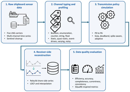
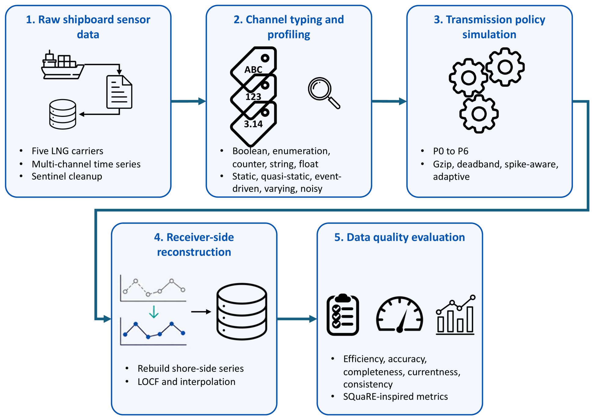
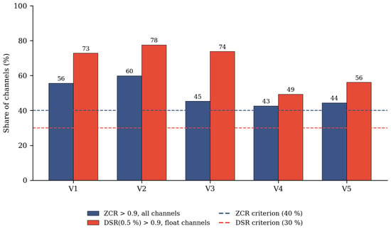
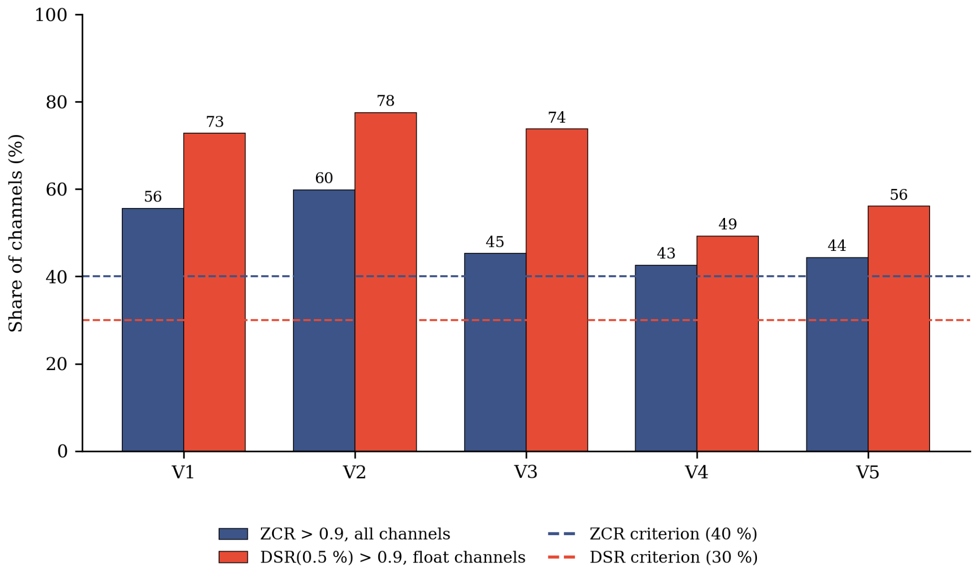
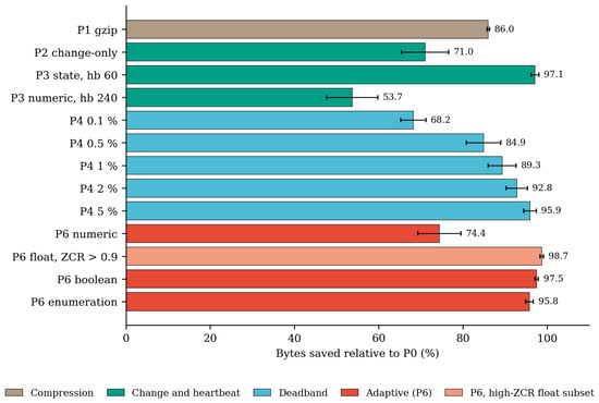
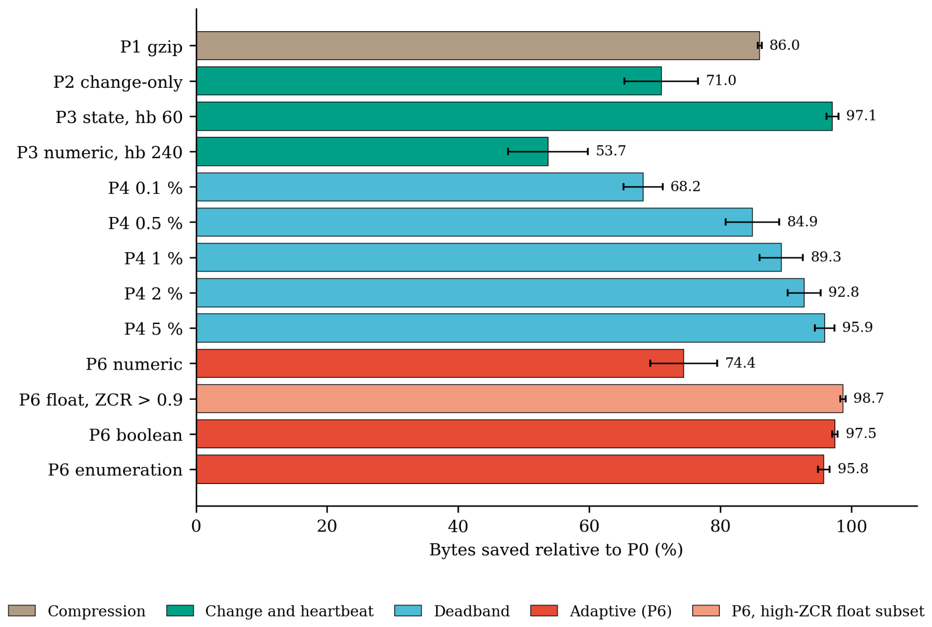
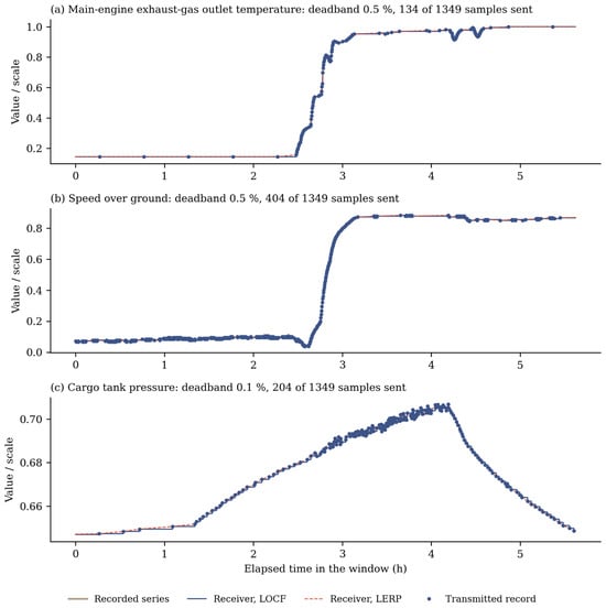
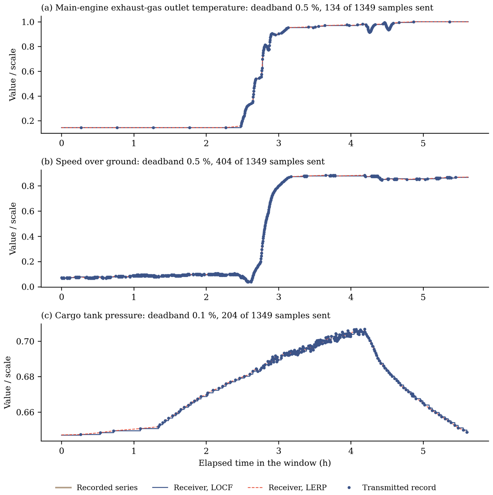
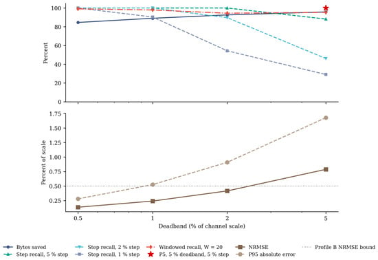
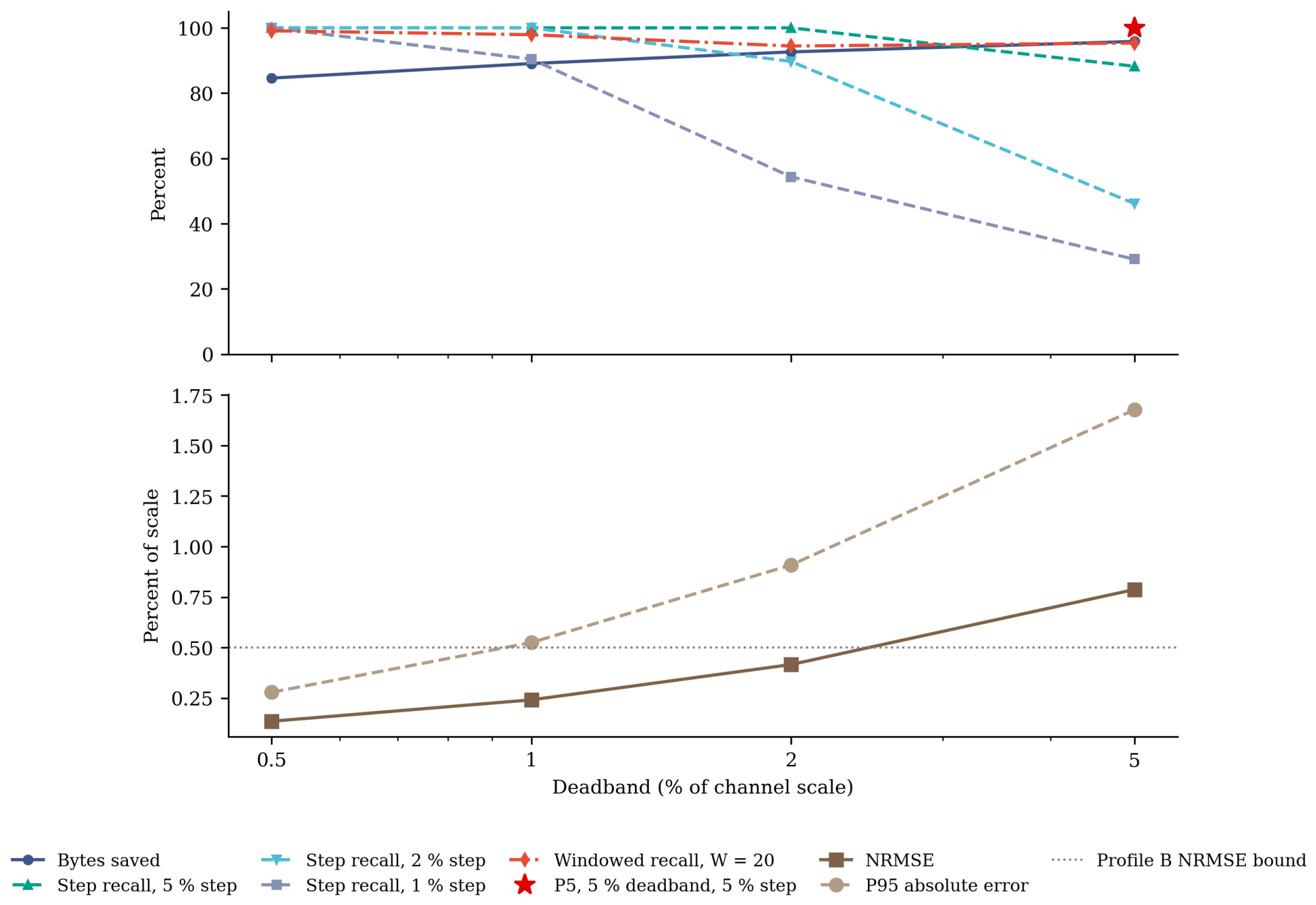
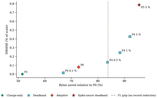
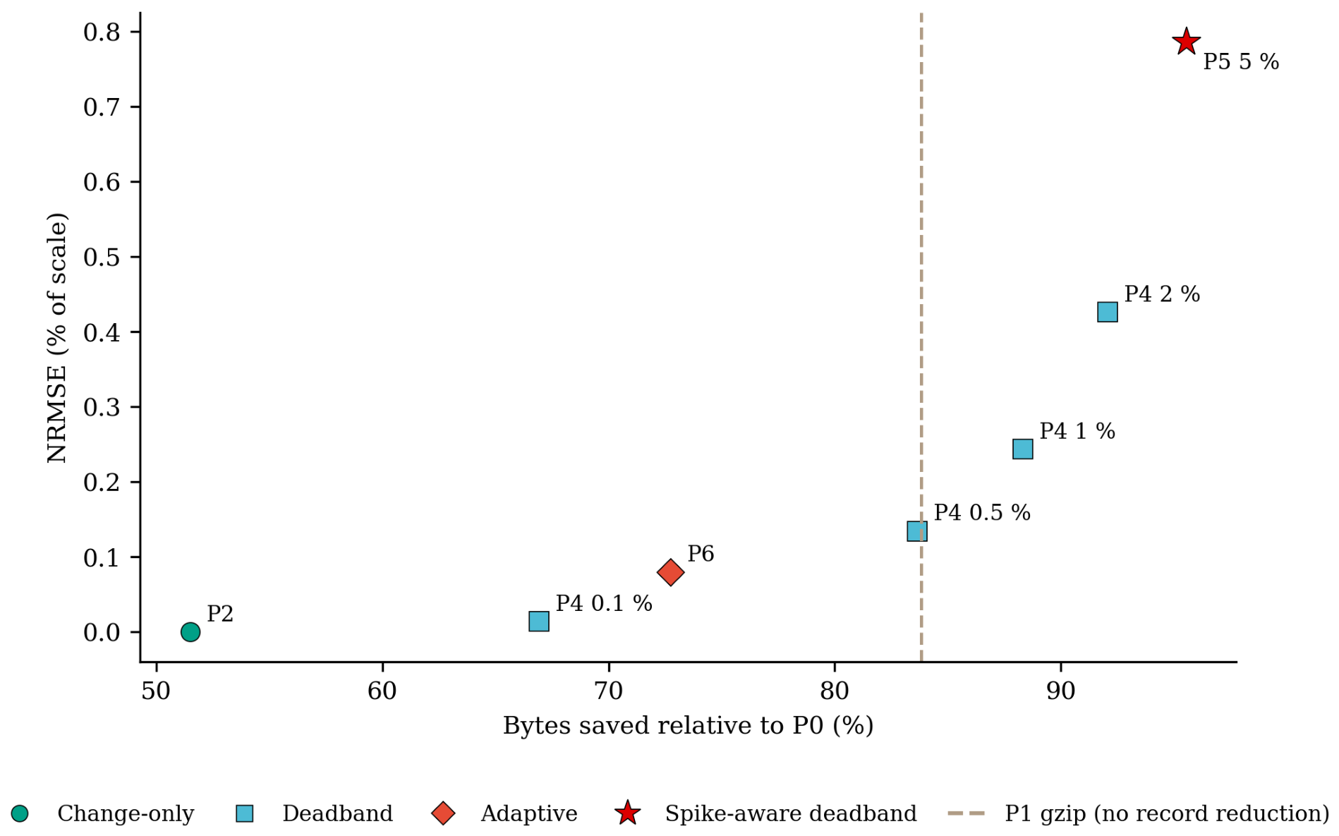

Disclaimer/Publisher’s Note: The statements, opinions and data contained in all publications are solely those of the individual author(s) and contributor(s) and not of MDPI and/or the editor(s). MDPI and/or the editor(s) disclaim responsibility for any injury to people or property resulting from any ideas, methods, instructions or products referred to in the content. |
© 2026 by the authors. Licensee MDPI, Basel, Switzerland. This article is an open access article distributed under the terms and conditions of the Creative Commons Attribution (CC BY) license.