Near-Offset Gap Reconstruction in Marine Seismic Data Using Global Amplitude Balancing Operator-Enhanced Seismic Interferometry

Abstract

Near-offset acquisition gaps are a common limitation in marine seismic surveys, where practical source–receiver configurations leave part of the short-offset wavefield unrecorded. The resulting loss of near-offset information can degrade wavefield continuity and reduce the reliability of subsequent seismic processing, subsurface imaging, and geological interpretation. Seismic interferometric reconstruction provides a data-driven approach to recovering the missing near-offset information by generating virtual traces from the recorded wavefield. However, conventional implementations generally rely on local matching filters to compensate for discrepancies between virtual and observed traces, which can introduce amplitude distortions and artifacts in the reconstructed data. To enhance reconstruction accuracy in the presence of near-offset gaps, we propose a novel global amplitude balancing operator (GABO)-enhanced interferometric reconstruction method. The GABO employs focal transformation to globally balance the wavefield along the offset direction by integrating and localizing reflection energy. A projection onto convex sets (POCS)-like iterative framework is further incorporated to improve reconstruction accuracy and robustness. Tests on both synthetic and field marine seismic datasets demonstrated that the proposed method outperforms conventional interferometric reconstruction, particularly in terms of amplitude fidelity, reconstruction accuracy, and offset continuity. The synthetic example showed that the mean correlation coefficient (CC) increased from 0.677 to 0.960, while the mean normalized root-mean-square error (NRMSE) decreased from 0.828 to 0.370 compared with conventional interferometric reconstruction. Furthermore, the method involves physically interpretable parameter selection and exhibits consistent iterative improvement in the synthetic tests.

1. Introduction

Marine seismic surveying is an important geophysical approach for imaging subseafloor structures and supporting marine geological investigations. In practical marine seismic acquisition, however, source–receiver geometry, acquisition configuration, and operational constraints can result in incomplete spatial sampling [1,2]. A typical example is the near-offset acquisition gap, in which part of the short-offset wavefield cannot be directly recorded because of the finite separation between the seismic source and the nearest available receiver [3,4]. Such incomplete sampling reduces wavefield continuity and spatial sampling integrity and may affect amplitude-variation-with-offset (AVO) analysis [5,6], geological attribute extraction, and subsequent seismic imaging [7,8]. Reliable reconstruction of missing near-offset information is therefore important for improving the completeness of marine seismic observations as well as the reliability of subsequent subsurface imaging and geological interpretation [9,10,11].

Diverse seismic data reconstruction methods have been developed, including predictive filtering approaches [12], compressive-sensing-based methods [13,14,15], wavefield propagation-based approaches [16] and transform-domain methods [17,18], and more recently, deep-learning-based reconstruction approaches [19,20,21]. These methods can broadly be considered in terms of interpolation and extrapolation [22]. In conventional interpolation problems, missing traces are generally surrounded by available observations, so the local kinematic or transform-domain structure of seismic events can be inferred from data on both sides of the missing positions. In contrast, a near-offset acquisition gap represents a boundary-extrapolation problem: no observations are available toward the zero-offset side of the missing region, and the reconstruction must extend event kinematics and amplitudes beyond the available acquisition support [23]. Consequently, the performance of transform- or sparsity-based methods depends more strongly on the available aperture, event curvature, and the ability of the chosen representation to extrapolate the observed wavefield toward shorter offsets. This makes near-offset reconstruction different from conventional interpolation of isolated or internally missing traces and motivates reconstruction approaches specifically designed for short-offset extrapolation [24].

Interferometric reconstruction presents significant advantages for data extrapolation, being fully data-driven and capable of utilizing multiple reflections for extra illumination, thereby correcting reconstruction results more effectively [25,26,27]. This method fills near-offset trace gaps in two stages: initially, virtual traces are generated through the cross-correlation of the existing dataset. This is then followed by aggregating these correlated results across various shot positions [28]. However, due to limitations such as the limited source–receiver aperture and restricted illumination [29,30], the reconstructed virtual traces may exhibit wavelet distortions, low signal-to-noise ratios (SNR), and non-physical events. These issues can render subsequent data processing methods less effective, potentially leading to decreased resolution and the emergence of false geological layers in imaging results.

To solve the challenges identified in interferometric reconstruction, most interferometric reconstruction methods employ a matching filter, known for its amplitude correction and noise suppression capabilities. As described by Hanafy [31], this filter is usually derived by trial-and-error within a time-space window, which generally extends over several wavelet lengths and covers a few traces. This approach suggests that the matching filter mainly attenuates reconstruction errors within a localized window. Its effectiveness hinges on the assumption of continuity (in terms of travel time, amplitude, etc.) between the original and virtual data in the offset direction within this window [32]. When facing large trace gaps, the limited source–receiver aperture required by seismic interferometry is more challenging [33,34,35]. This difficulty can damage, or even break, the continuity between virtual and original trace, resulting in the final reconstruction still suffering from amplitude distortion and artifacts.

To address this limitation, we propose a global amplitude balancing operator (GABO)-enhanced seismic interferometric reconstruction method for marine near-offset gaps. The innovation of this method lies in formulating the focusing and energy redistribution properties of the focusing transform into a global amplitude balancing operator and embedding it within an iterative interferometric reconstruction framework. In each iteration, the reconstructed wavefield is transformed into the focal domain, where reflection energy is localized and reconstruction artifacts are separated according to their different focal-domain distributions. The balanced wavefield is then used to update the missing near-offset data in a POCS-like framework [36,37]. In this way, amplitude correction is performed using wavefield information over a broader spatial extent rather than relying solely on local matching between adjacent traces. Synthetic and field marine seismic examples are used to evaluate the reconstruction accuracy, amplitude fidelity, and applicability of the proposed method.

The remainder of this paper is organized as follows. The Methods Section starts with an overview of the traditional interferometric reconstruction and the focal transformation. Following this, we introduce the GABO-based interferometric reconstruction. The Results Section illustrates the effectiveness of our proposed method through both synthetic and field marine seismic dataset. Finally, the paper concludes by providing a discussion of the method’s limitations and concluding remarks.

2. Methods

2.1. Conventional Interferometric Reconstruction Methods

Seismic interferometric reconstruction can transform multiples into missing signals by calculating the cross-correlation of records at different receivers [38,39]. Derived from the reciprocity theorem, the equation of interferometric reconstruction is given as follows [40]:

$$\begin{array}{l}G({\mathit{L}}_B|{\mathit{L}}_A,\omega )-G({\mathit{L}}_A|{\mathit{L}}_B,\omega {)}^{*}\\ ={\int }_{S_0+S_{\infty }}[G({\mathit{L}}_B|\mathit{L},\omega {)}^{*}{\displaystyle \frac{\partial G\left({\mathit{L}}_A|\mathit{L},\omega \right)}{\partial \mathbf{n}}}-G({\mathit{L}}_A|\mathit{L},\omega ){\displaystyle \frac{\partial G({\mathit{L}}_B|\mathit{L},\omega {)}^{*}}{\partial \mathbf{n}}}]d^2\mathit{L}\\ \approx {\int }_{S_0}[G({\mathit{L}}_B|\mathit{L},\omega {)}^{*}{\displaystyle \frac{\partial G\left({\mathit{L}}_A|\mathit{L},\omega \right)}{\partial \mathbf{n}}}-G({\mathit{L}}_A|\mathit{L},\omega ){\displaystyle \frac{\partial G({\mathit{L}}_B|\mathit{L},\omega {)}^{*}}{\partial \mathbf{n}}}]d^2\mathit{L}\\ {\mathit{L}}_A,{\mathit{L}}_B\in S_0^{\prime };\end{array}$$

(1)

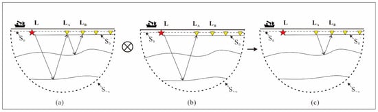
As shown in Figure 1, L_A is the location where source is excited, L_B is the location of receivers, G(L_B|L_A,ω) is the Green’s function in frequency domain, and ω is the angular frequency [41]. S₀ and $S_0^{\prime }$ represent the surface where the source and receivers are distributed, respectively. Here, S₀ and $S_0^{\prime }$ denote the source and receiver surfaces, respectively, whereas S_∞ represents a semicircular boundary at infinity. According to Wappenaar [42], in cases where the medium exhibits sufficient heterogeneity, it becomes feasible to disregard the integration over S_∞. ∗ represents complex conjugate, n is the normal direction.

Figure 1. Ray diagram for transforming multiples into primaries by interferometric reconstruction. This process involves creating virtual traces, as shown in (c), by cross-correlating the records from receiver in (a) with those from receiver in (b).

Through the far-field approximation, Equation (1) can be written as

$$\begin{array}{l}G\left({\mathit{L}}_B\right|{\mathit{L}}_A,\omega )-G({\mathit{L}}_B|{\mathit{L}}_A,\omega {)}^{*}\\ \approx 2\mathit{ik}{\int }_{S_0}\left[G\right({\mathit{L}}_B|\mathit{L},\omega {)}^{*}G\left({\mathit{L}}_A\right|\mathit{L},\omega \left)\right]d^2\mathit{L}\\ {\mathit{L}}_A,{\mathit{L}}_B\in S_0^{\prime };\end{array}$$

(2)

where k is wavenumber. Equation (2) in time-space domain is

$$\begin{array}{l}G\left({\mathit{L}}_B\right|{\mathit{L}}_A,t)+G({\mathit{L}}_A|{\mathit{L}}_B,-t)\\ \approx {\int }_{S_0}\left[G\right({\mathit{L}}_B|\mathit{L},t)\otimes G({\mathit{L}}_A|\mathit{L},t)]d^2\mathit{L}\\ {\mathit{L}}_A,{\mathit{L}}_B\in S_0^{\prime };\end{array}$$

(3)

where ⊗ represents cross-correlation. Figure 1 explains how to use Equation (3) to transform multiples into primaries by the cross-correlation method. By canceling overlapping paths, the virtual primaries G(L_B|L_A,t) are reconstructed, which have similar kinematic characteristics with the original primaries; hence, they can be used for filling the near-offset gap.

However, due to the use of far-field approximation in the calculation process and the limitation of the acquisition aperture, the virtual traces are usually different from the original trace. In order to mitigate these differences, the conventional method is employed using 1D least-squares matching filter to match the virtual trace to the original traces [43]. Specifically, the filter is estimated by matching the virtual trace G^V(L_B|L_A,ω) to an available observed reference trace G^ref(L_B|L_A,ω). The observed reference trace is a known trace and is distinguished from the final reconstructed trace. After the matching filter is estimated, the final reconstructed trace is obtained as

G^R(L_B|L_A,ω) = G^V(L_B|L_A,ω)W(ω),

(4)

where G^R(L_B|L_A,ω) is the final reconstruction trace, G^V(L_B|L_A,ω) is the virtual trace before matching. W(ω) is the matching filter which is defined in Equation (5):

$$W(\omega )={\displaystyle \frac{G^V\left({\mathit{L}}_B\right|{\mathit{L}}_A,\omega {)}^{*}{G}^{\mathit{ref}}\left({\mathit{L}}_B\right|{\mathit{L}}_A,\omega )}{G^V\left({\mathit{L}}_B\right|{\mathit{L}}_A,\omega {)}^{*}{G}^V\left({\mathit{L}}_B\right|{\mathit{L}}_A,\omega )+\epsilon }}$$

(5)

where G^ref(L_B|L_A,ω) denotes the observed reference trace used to estimate the matching filter and ε′ represents the damping factor. Generally, both virtual and original traces are segmented into overlapping patches for the better performance of the matching filter. For each local matching window, the available observed traces adjacent to the missing region are used to define the reference data G^ref(L_B|L_A,ω), so that the matching is constrained by the local continuity between the virtual and observed wavefields. For the datasets considered in this study, the matching-filter length was uniformly set to 101 samples and the time-window length to 220 samples. Adjacent windows were shifted by 201 samples, corresponding to an overlap of 19 samples, and the damping factor ε′ was set to 0.1. These parameter values were used consistently throughout the experiments in this study. In other datasets, they may be adjusted according to the temporal sampling and wavelet characteristics of the data.

In summary, interferometric reconstruction obtains virtual traces by canceling overlapping paths of primaries and multiples. Subsequently, a matching filter is adopted to mitigate the differences. In this paper, we denote this process as follows:

$$G^R=\mathit{WR}(G^{\mathit{obs}},G_p^{\mathit{obs}}),$$

(6)

where $\mathit{R}(G^{\mathit{obs}},G_p^{\mathit{obs}})$ represents the process of interferometric reconstruction using observed data G^obs and the primary of the observed data $G_p^{\mathit{obs}}$. W represents the application of a matching filter.

2.2. Focal Transformation

As mentioned above, traditional interferometric reconstruction methods rely on the matching filter to mitigate the difference between the virtual trace and the original trace within a local window [31]. However, due to the lack of original data, the matching process can only choose adjacent traces as approximate substitutes [32], which means, as the distance between the virtual trace and the reference trace increases, the effectiveness of the matching filter will gradually decrease [44]. It means that, when facing the seismic data with a large offset gap, the quality of the reconstructed trace is still reduced due to the limited acquisition aperture, which decreases the reliability of subsequent seismic data processing and interpretation. The focal transformation can integrate reflection information of the entire wavefield and separate artifacts from signals. This offers the potential to attenuate the difference in the virtual trace, caused by far-field approximation and the limited acquisition aperture. In this section, we review focal transformation in detail.

The focal transformation [45] method necessitates organizing the dataset into a structured data matrix. This involves arranging shot gathers into a three-dimensional data cube, ordered by shot, receiver, and time. By applying a time-domain Fourier transformation, we can transform this data cube into a frequency-domain data matrix as follows:

$$\mathit{D}(\omega )=\left[\begin{array}{ccccc}\mathit{D}\left(L_1\right|L_1,\omega )& ...& \mathit{D}\left(L_1\right|L_j,\omega )& ...& \mathit{D}\left(L_1\right|L_n,\omega )\\ ...& ...& ...& ...& ...\\ \mathit{D}\left(L_i\right|L_1,\omega )& ...& \mathit{D}\left(L_i\right|L_j,\omega )& ...& \mathit{D}\left(L_i\right|L_n,\omega )\\ ...& ...& ...& ...& ...\\ \mathit{D}\left(L_n\right|L_1,\omega )& ...& \mathit{D}\left(L_n\right|L_j,\omega )& ...& \mathit{D}\left(L_n\right|L_n,\omega )\end{array}\right],$$

(7)

where D(ω) denotes the data cube’s frequency slice ω, with L_i and L_j indicating the positions of receivers and sources, respectively. Additionally, n is the total count of shot gathers. The data matrix structure, as illustrated in Equation (7), is organized such that each row corresponds to a receiver gather and each column corresponds to a shot gather.

In the focal domain, effective signals can be compressed to the focal point, making a significant difference between the distribution areas of effective signals and noise. The forward and inverse transformation pair are

Q = FD(ω)

(8)

D(ω) = PQ

(9)

where Q is focal domain coefficients, F = P⁻¹. In practice, the focal operator F is not obtained through a direct matrix inverse. Instead, a regularized least-squares pseudoinverse is used to stabilize the transformation:

F ≈ P^H[PP^H + ε²I]⁻¹

(10)

where ε denotes the stabilization parameter used in the regularized least-squares inversion of the focal transformation. In the experiments presented in this study, ε is set to 0.1. P can be chosen as the primary. By substituting Equation (10) into Equation (8), Equation (11) is obtained as

$$\mathit{Q}={\mathit{P}}^H{\left[\mathit{P}{\mathit{P}}^H+{\epsilon }^2\mathit{I}\right]}^{-1}\mathit{D}\left(\omega \right)$$

(11)

For convergence acceleration, the weighted least-squares problem can be reformulated into an optimization problem [46]. In this way, a linear system for focal transformation is defined as follows:

Ax = f^HBlockDiag_ω(P⊗I)fx = f^Hd(ω) = d

(12)

where x represents the focal coefficient vector, f^H and f are the Fourier transform pair, ⊗ is the Kronecker product, I is the identity matrices, and d is the vector of data D in the physical domain. In this way, A is the linear operator which can transform the data from the focal domain into the physical domain; it can be considered as a combination operator of inverse focal transformation operator P and the Fourier transform pair.

Based on Equation (12), the seismic wavefield in the focal domain can be further expressed through the following sparsity-constrained formulation:

$$\widehat{x}=\mathit{arg}\underset{x}{\mathit{min}}{‖x‖}_1\mathrm{s}.\mathrm{t}.{‖\mathit{A}x-d‖}_2\le \sigma$$

(13)

where ‖‖₁, ‖‖₂ represent the determination of L1 and L2 norms and σ denotes the tolerance used in the sparse focal-domain inversion. In this study, σ was fixed at 10% of the L2 norm of the data.

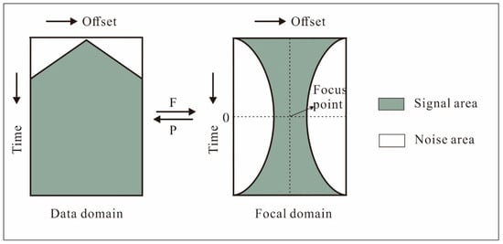
The focal transformation technique employs spatial phase reduction of reflection events to integrate and localize the reflection data from the entire wavefield [47]. This transformation can be regarded as a weighted auto-correlation, effectively removing the spatial phase while concentrating the spatial amplitude. After the application of the forward focal transformation, it results in the effective signals being amassed at the focal point. This characteristic is fundamental in decomposing the focused signal from noise, as depicted in Figure 2. Furthermore, during the forward and inverse focal transformation process, the amplitude of the reflection events is concentrated and then redistributed; this can be considered as the amplitude balancing process.

Figure 2. Demonstration of focal domain: The focal transform localizes the non-aliased signal energy around its focus point and disperses the aliased signal and coherent noise away from its focal area.

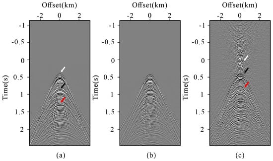
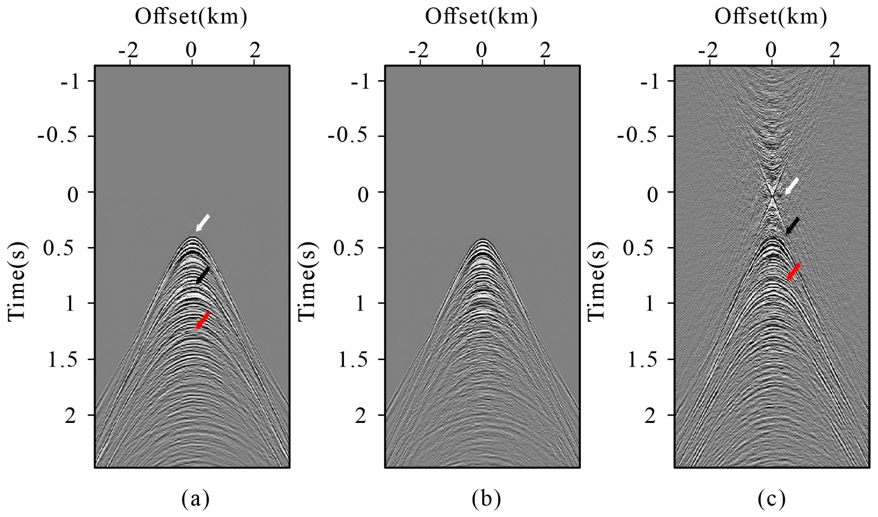
For better understanding of this process, we performed a focal transformation shown in Figure 3, demonstrating the differences between the same data in the physical domain and the focal domain. Figure 3a shows the physical domain; in order to better demonstrate the transformation of the reflection events, in Figure 3a, primaries are marked by a white arrow, first-order multiples are marked by a black arrow, and a red arrow is used to indicate the second-order multiples. Figure 3b shows the focal operator used in the transformation which is the primary of the data in Figure 3a obtained by the surface-related multiple elimination (SRME) method [48]. Figure 3c shows the data in the focal domain, and events are highlighted using identical colors as those in Figure 3a. By comparing Figure 3a and Figure 3c, it is evident that reflection information matches the spatial phase of the operator, leading to phase reduction in the focal domain: primary is concentrated as a focal point, the first-order multiples are reordered as primaries, and the second-order multiples are transformed into first-order multiples, respectively. In conclusion, the focal transformation has two main features [44]. First, it can separate effective signals from artifacts through phase reduction. Second, the energy concentration and redistribution process can balance event amplitudes and reduce amplitude distortion. These features provide the basis to solve the problem of inconsistency between the virtual trace and the original trace.

Figure 3. Demonstration of the mechanism of focal transformation: (a) original data; (b) focal operator; (c) focal domains of the data associated with (a).

2.3. GABO-Enhanced Iterative Interferometric Reconstruction

As in the demonstration, the complete seismic data D are related to the observed data D^obs and observation matrix O:

D^obs = OD.

(14)

The acquisition operator O is a binary sampling mask, whose elements equal 1 at the recorded source–receiver positions and 0 within the missing near-offset region. The observed data are therefore expressed by using the conventional interferometric reconstruction defined in Equation (6) together with the observation model in Equation (14). The reconstructed data can be expressed as

D = D^obs + (I − O)D^R

(15)

D^R represents the conventional interferometric reconstructed trace, and it is defined in Equation (6) that ${\mathit{D}}^R=\mathit{WR}({\mathbf{D}}^{\mathit{obs}},{\mathit{D}}_p^{\mathit{obs}})$. I represents the identity matrix. As for the advantages of focal transformation, we build a global amplitude balancing operator (GABO) and refer to the POCS algorithm to establish an iterative framework. Equation (15) is rewritten as

$${\tilde{\mathit{D}}}^n={\mathit{D}}^{\mathit{obs}}+(\mathit{I}-\mathit{O}){\mathit{B}}^n{\mathit{u}}^n$$

(16)

$${\mathit{u}}^n=\mathit{WR}[{\mathit{D}}^{n-1},{\mathit{D}}_p^{n-1}]$$

(17)

where ${\tilde{\mathit{D}}}^n$ represents the final reconstruction result, uⁿ denotes the interferometric prediction generated from the reconstructed full-wavefield data Dⁿ⁻¹ and primary-wave data ${\mathit{D}}_p^{n-1}$ of the previous iteration, W represents the matching filter, $\mathit{R}[{\mathit{D}}^{n-1},{\mathit{D}}_p^{n-1}]$ represents the interferometric reconstruction using the n − 1 iteration of the reconstruction full data and primary data. To improve the stability of the iterative update, a relaxation-based data-consistency step is applied after each interferometric prediction. Let ${\tilde{\mathit{D}}}^n$ denote the reconstructed wavefield obtained at the n-th iteration before data-consistency relaxation. The updated wavefield is then expressed as

$${\mathit{D}}^n={\tilde{\mathit{D}}}^n+{\alpha }_n({\mathit{D}}^{\mathit{obs}}-{\tilde{\mathit{D}}}^n),{\alpha }_n={\displaystyle \frac{n}{N+1}}$$

(18)

where Dⁿ represents the updated reconstruction result, n is the current iteration index, and N is the prescribed total number of iterations. Therefore, the data-consistency weight at a given iteration depends on both the current iteration index and the prescribed total number of iterations. In Equation (16), Bⁿ is the GABO, and to attenuate the reconstruction error of artifacts and amplitude distortion, it is defined as

$${\mathit{B}}^n=\mathit{A}{\mathit{T}}_n{\mathit{A}}_{\gamma }^{†}$$

(19)

where A denotes the synthesis operator introduced in Section 2.2, T_n is a threshold operator, and ${\mathit{A}}_{\gamma }^{†}$ denotes the corresponding regularized analysis operator. The subscript γ indicates that the transformation from the physical domain to the focal domain is stabilized by the regularization parameter γ. Accordingly, the GABO first maps the physical-domain wavefield into focal-domain coefficients through ${\mathit{A}}_{\gamma }^{†}$, applies the threshold operator T_n to attenuate the dispersed artifact energy, and then maps the processed coefficients back to the physical domain through A. In the numerical implementation, ${\mathit{A}}_{\gamma }^{†}$, is not explicitly assembled as a dense pseudo-inverse matrix. Instead, its action is evaluated independently for each frequency slice through a stabilized least-squares solution. Specifically, the focal-domain coefficient vector is obtained by solving

$$(G_{\omega }^H{G}_{\omega }+\mu n^r\mathbf{I})x_{\omega }=G_{\omega }^H{d}_{\omega }$$

(20)

where G_ω denotes the focal operator at frequency ω, the superscript H denotes the conjugate transpose, d_ω is the corresponding data at that frequency, n^r is the number of receivers, I is the identity matrix, and μ is the stabilization factor. In this study, μ is set to 0.1. Solving Equation (20) yields the focal-domain coefficients x_ω without explicitly forming the inverse matrix. These coefficients are subsequently processed by T_n and mapped back to the physical domain through A.

Accordingly, the focal-domain threshold operator T_n is implemented using a discrete sector mask. Let i and j denote the horizontal and vertical sample indices in the focal domain, respectively, and let (i_c,j_c) denote the focal center. The signal-preserving sector is then defined as

$${\mathit{T}}_n(i,j)=\left\{\begin{array}{cc}1,& \left|i-i_c\right|\le {\omega }_0+{\varsigma }_n\left|j-j_c\right|\\ 0& \mathit{otherwise}\end{array}\right.,$$

(21)

where ω₀ denotes the minimum half-width of the preserved region at the focal center, and ς_n is a dimensionless parameter controlling the widening rate of the sector away from the focal center. In this study, ω₀ was set to 2 samples. Because the mask is defined directly on discrete focal-domain indices, no division by time or offset is involved and no singularity occurs at zero time. For ς_n = 0.20, the horizontal half-width of the preserved sector increases by 0.20 sample for each one-sample displacement in the vertical focal-domain direction. The value of ς_n was selected by examining the outer boundary of the coherent focused reflection energy in the focal domain. The shallowest coherent reflection provides a physical guide for defining the limiting signal-preserving boundary. For the datasets considered in this study, ς_n = 0.20 was adopted and kept fixed during the corresponding reconstruction. The value adopted in each experiment is specified in the corresponding example.

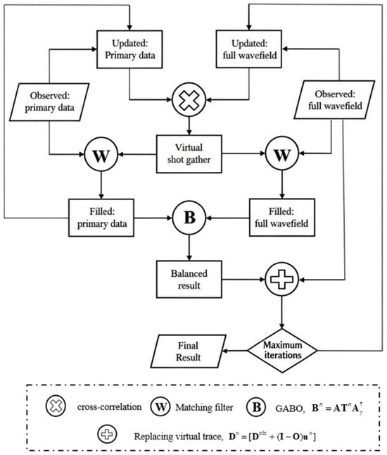
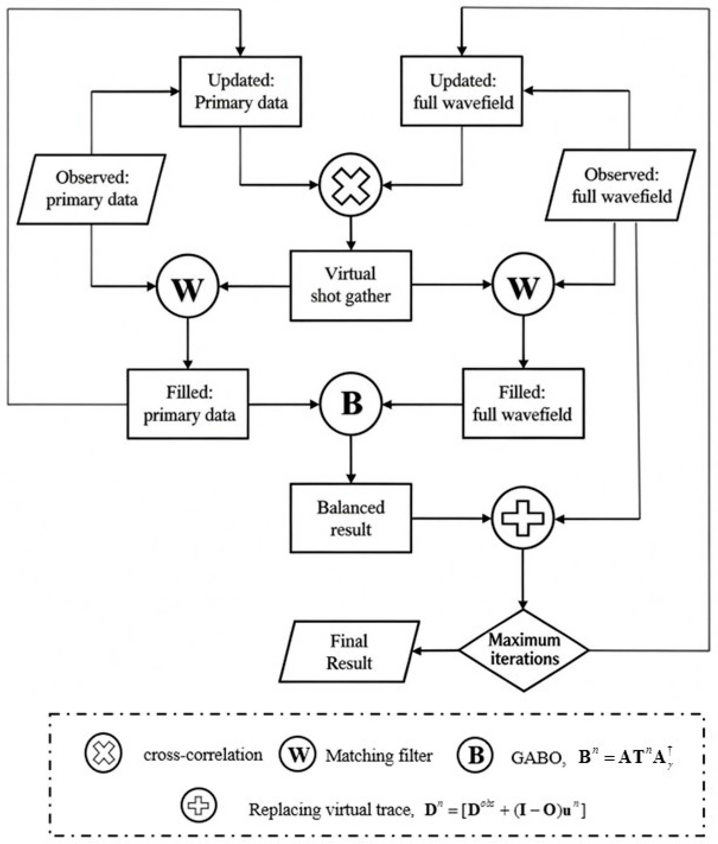
The complete process of the iterative interferometric reconstruction method based on GABO is as shown in Figure 4. For reproducibility, the matching-filter damping factor was set to 0.1, and the focal-transformation stabilization factor was set to 0.1. The dimensionless focal-domain sector-opening parameter ς_n was set to 0.20, with a minimum focal-center half-width ω₀ of 2 samples. The sector boundary was selected with reference to the outer envelope of the coherent focused reflection energy in the focal domain. The main reconstruction used three iterations. For all experiments reported in this study, the sparsity tolerance was consistently set to 10% of the L2 norm of the data.

Figure 4. Basic flow of the global amplitude balancing operator (GABO)-enhanced interferometric reconstruction method.

3. Results

3.1. Synthetic Example

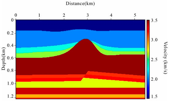
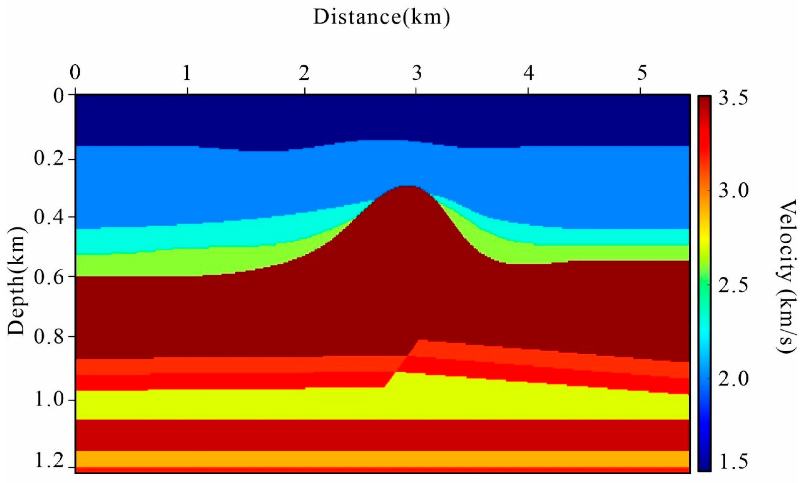
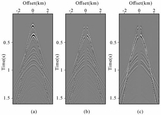
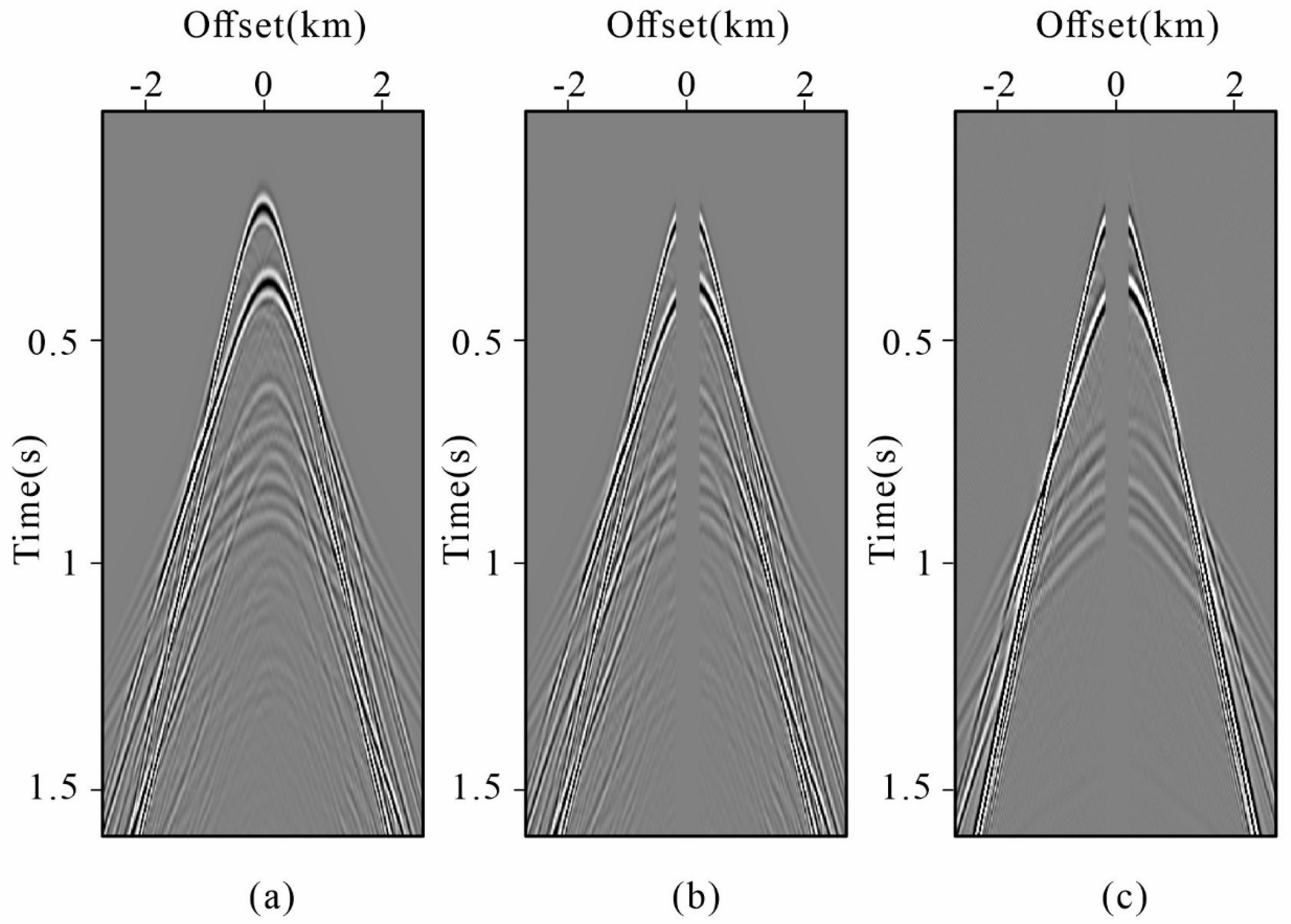
We first evaluate the proposed method using synthetic data generated from the salt dome velocity model [49,50], as shown in Figure 5. The acquisition geometry consists of 271 sources and 271 receivers, both uniformly spaced at 20 m. The recording time is 1.6 s with a temporal sampling interval of 2 ms. The modeled full-wavefield data are shown in Figure 6a, in which surface-related multiples are clearly visible. Subsequently, in order to obtain the near-offset gap, which is typical in streamer marine data, we remove the traces with absolute offsets smaller than 200 m from both modeled data as shown in Figure 6b. Considering the principle of the interferometric reconstruction method, we also found that the primary data contains near-offset gap as shown in Figure 6c.

Figure 5. Salt dome velocity model.

Figure 6. Demonstration of the synthetic data: (a) the original shot gather; (b) the original shot gather with near-offset gap; (c) the primaries with near-offset gap.

The synthetic evaluation consists of four complementary tests. First, the proposed method is compared visually with radon-based reconstruction, curvelet-based sparse reconstruction, and conventional interferometric reconstruction. Second, difference sections and trace-level comparisons are used to examine the waveform and amplitude fidelity. Third, quantitative reconstruction accuracy is evaluated over all deliberately removed near-offset traces using CC [51], mean squared error (MSE) [52], and NRMSE. Finally, the effects of iteration number and near-offset gap size are examined to evaluate the behavior of the proposed method under different reconstruction conditions.

For each deliberately removed trace, CC measures waveform similarity, MSE measures the absolute reconstruction error, and NRMSE normalizes the reconstruction error by the energy of the corresponding reference trace. A higher CC and lower MSE/NRMSE indicate better reconstruction. All three metrics are calculated trace by trace and subsequently summarized using their mean and standard deviation:

$$\mathrm{CC}=\frac{{\sum }_m{\sum }_n\left(A_{\mathit{mn}}-\overline{A}\right)\left(B_{\mathit{mn}}-\overline{B}\right)}{\sqrt{{\sum }_m{\sum }_n(A_{\mathit{mn}}-\overline{A}{)}^2{\left(B_{\mathit{mn}}-\overline{B}\right)}^2}}$$

(22)

$$\text{MSE}=\frac{1}{n}\sum _{i=1}^n(A_i-B_i{)}^2$$

(23)

$$\text{NRMSE}=\frac{{\left||\mathbf{A}-\mathbf{B}|\right|}_2}{{\left|\left|\mathbf{A}\right|\right|}_2}$$

(24)

where A denotes the real trace, and B is the predicted trace. $\overline{A}$ and $\overline{B}$ are the average of A and B.

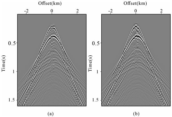
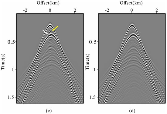
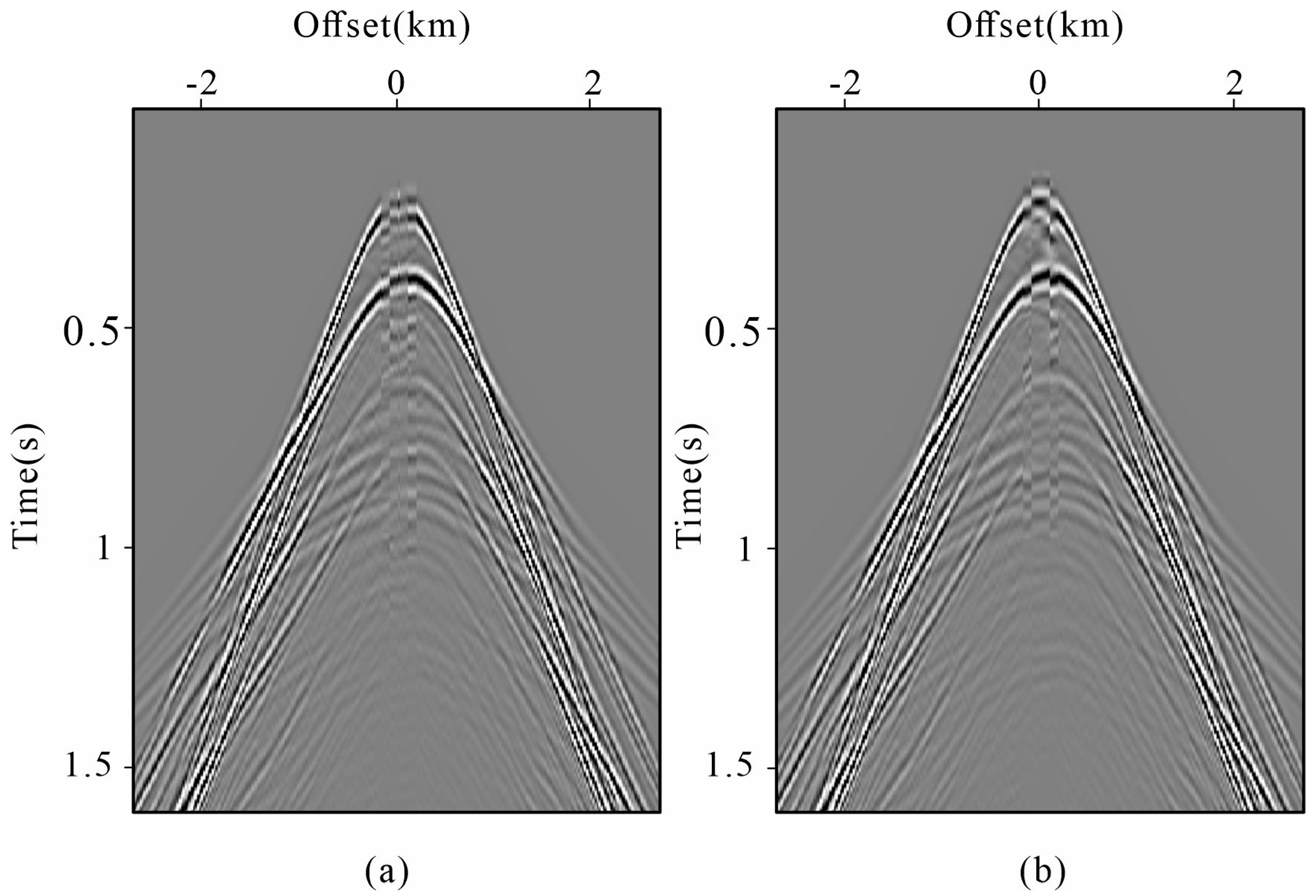
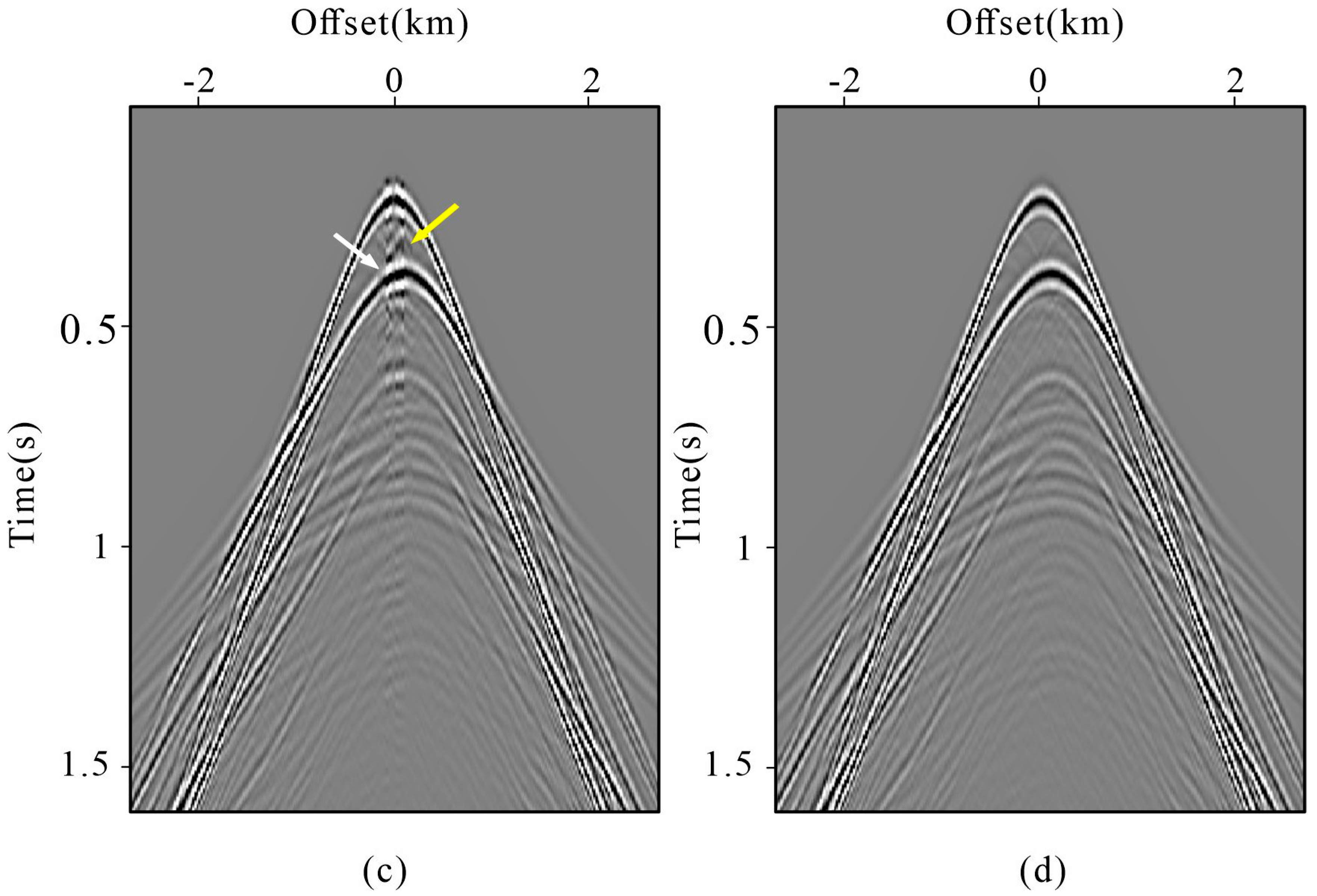
Figure 7 shows the reconstructed result of four different methods. Within the control groups, we picked three classic reconstruction methods for comparison. These included two reconstruction methods: the radon-based reconstruction method [53], and the curvelet-based sparse reconstruction method [54], alongside an extrapolation method, the conventional interferometric reconstruction method [28]. The radon- and curvelet-based baseline methods were implemented using standard formulations with conventional settings. For the parabolic radon reconstruction, the curvature parameter q was uniformly sampled from −0.25 to 0.25 s/km² using 501 samples, whereas the curvelet reconstruction used three decomposition scales with four angular directions. For both methods, the normalized sparsity threshold was set to 0.05 of the maximum transform-coefficient magnitude. All methods were applied to the same input data and missing-trace mask to ensure a consistent comparison. The near-offset gap reconstruction results of two reconstruction methods are shown in Figure 7a,b. When we compare these methods to the interferometric method and proposed method shown in Figure 7c,d, we notice a degradation in the quality and accuracy of the generated reconstruction. Specifically, in Figure 7a,b, a considerable amount of phase distortions along the events is observable in the reconstruction results obtained by the reconstruction methods. These phase distortions result in poor continuity of the reconstructed events, which potentially affect the accuracy of subsequent seismic analysis. The conventional interferometric method provides improved event continuation (Figure 7c), reflecting the advantage of using multiple-reflection information for virtual-wavefield construction. However, an analysis of Figure 7c reveals two distinct problems when comparing the conventional interferometric reconstruction method to the proposed method shown in Figure 7d. Specifically, there is a significant amplitude discrepancy between the reconstructed and original traces, as indicated by the white arrows, alongside the presence of artifacts, as highlighted by the yellow arrows. These observed problems collectively underscore the effectiveness of the proposed method in facing near-offset reconstruction challenges.

Figure 7. Comparison of the synthetic data reconstruction results: (a) using radon-based reconstruction method; (b)using curvelet-based sparse reconstruction method; (c) using conventional interferometric reconstruction method; (d) using the proposed method.

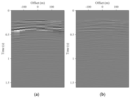
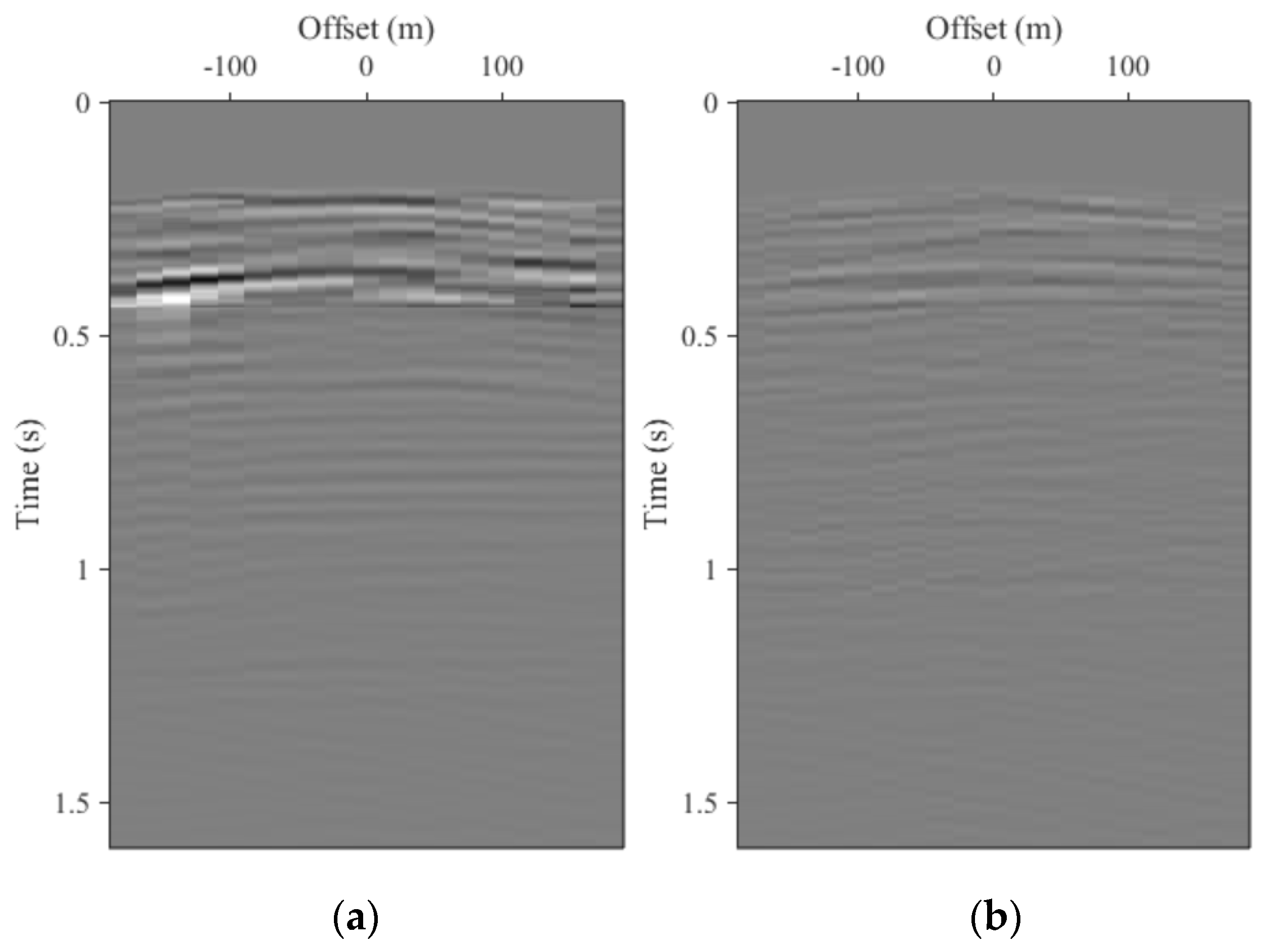
To further examine the reconstruction errors within the missing near-offset region, Figure 8 shows the residual sections obtained by subtracting the reference data from the conventional and proposed reconstruction results. Both residual sections are displayed using the same amplitude scale. The conventional interferometric reconstruction exhibits relatively strong residual energy, particularly around 0.3–0.5 s, indicating noticeable waveform and amplitude mismatch. In contrast, the residual energy of the proposed method is substantially reduced and more uniformly distributed, indicating improved waveform and amplitude fidelity in the reconstructed near-offset region. The additional computational overhead primarily stems from the focal-domain transformation and iterative updates. For this synthetic case, three iterations took 119.32 s, whereas conventional interferometric reconstruction under identical computational conditions took approximately 45.86 s.

Figure 8. Difference sections between the reconstructed and reference data within the missing near-offset region: (a) conventional interferometric reconstruction minus reference data; (b) proposed reconstruction minus reference data. Both panels are displayed using the same amplitude scale.

Quantitative evaluation was performed over all deliberately removed near-offset traces. As summarized in Table 1, the proposed method yields a higher mean CC and a lower standard deviation of CC compared with the conventional method. Meanwhile, both the mean MSE and mean NRMSE are reduced using the proposed method. The standard deviations of MSE and NRMSE are also smaller for the proposed scheme. The reduced standard deviations further indicate that the improvement is consistent across the missing traces rather than being limited to a small subset of the data.

Table 1. Quantitative reconstruction accuracy over all deliberately removed near-offset traces in the synthetic example.

Method	Mean CC	Std CC	Mean MSE	Std MSE	Mean NRMSE	Std NRMSE	Ntrace
Conventional	0.677	0.227	2.01 × 10−4	3.14 × 10−4	0.828	0.349	5059
Proposed	0.960	0.0273	3.52 × 10−5	2.59 × 10−5	0.370	0.181	5059

The iteration-by-iteration evolution of the reconstruction was further examined using a single six-iteration run. As shown in Table 2, the reconstruction accuracy improves progressively from the first to the sixth iteration. Because the relaxation weight α = n/(N + 1) depends on the prescribed total number of iterations N, the third iteration within this six-iteration run is not numerically equivalent to the final third iteration of the main reconstruction performed with N = 3. The mean CC rises from 0.619 after the first iteration to 0.968 after six iterations, accompanied by a reduction in mean NRMSE from 0.866 to 0.285. The performance gain is most pronounced in the early iterations and gradually diminishes as the reconstruction converges. For the main synthetic experiments, N = 3 was adopted as the prescribed total iteration number to balance reconstruction quality and computational cost.

Table 2. Iteration-by-iteration evolution within a six-iteration synthetic near-offset reconstruction.

Iteration	Mean CC	Mean MSE	Mean NRMSE
1	0.619	1.95 × 10−4	0.866
2	0.742	1.36 × 10−4	0.718
3	0.831	9.20 × 10−5	0.589
4	0.894	5.70 × 10−5	0.472
5	0.94	3.10 × 10−5	0.365
6	0.968	1.70 × 10−5	0.285

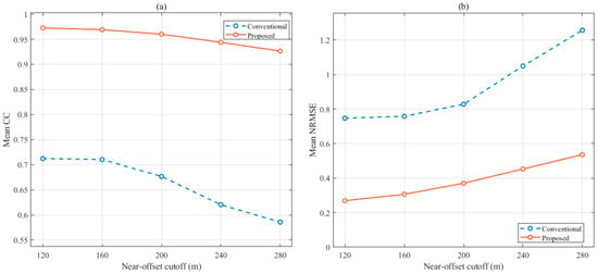
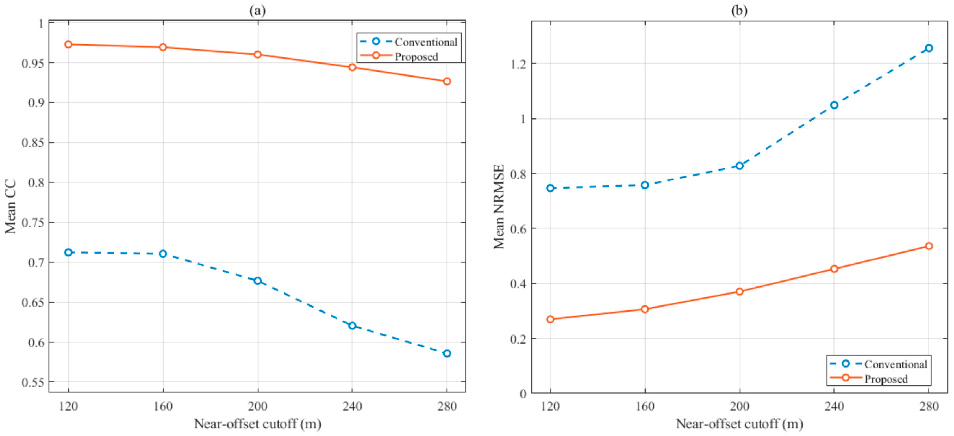
To further evaluate the influence of the missing near-offset range, additional tests were performed using near-offset cutoffs of 120, 160, 200, 240, and 280 m. Figure 9 shows that reconstruction accuracy decreases gradually as the missing region expands, as expected for an increasingly difficult extrapolation problem. Nevertheless, the proposed method consistently maintains higher CC and lower NRMSE than conventional interferometric reconstruction over the tested range. This result indicates that the improvement provided by GABO is not restricted to the 200 m cutoff used in the main synthetic example.

Figure 9. Reconstruction performance for different near-offset cutoffs: (a) mean CC; (b) mean NRMSE.

3.2. Field Marine Seismic Example

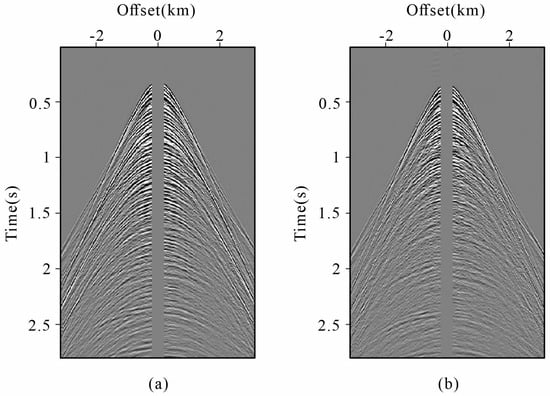
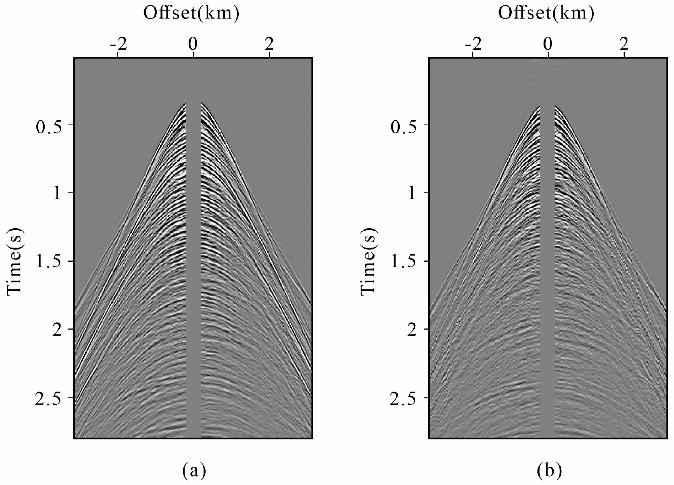
To validate the applicability of the proposed method to marine seismic surveys, we further tested it using a field marine seismic dataset containing a persistent near-offset acquisition gap. Figure 10a shows the 190th shot of the field data. The data were acquired at a water depth of approximately 300 m, with shot and receiver spacings of 25 m and a maximum offset of approximately 3150 m. The temporal sampling interval is 4 ms, the record length is 2.4 s, and the dominant frequency is approximately 20 Hz. A persistent near-offset acquisition gap of approximately 175 m is present throughout the dataset, providing a representative field case for evaluating the reconstruction of missing short-offset wavefield information. Prior to reconstruction, the field data were subjected to basic amplitude-preserving preprocessing, including bad-trace editing, broad band-pass filtering, and attenuation of isolated high-amplitude noise. The original 25 m source–receiver sampling and the approximately 175 m near-offset acquisition gap were retained throughout the processing. The auxiliary primary-wavefield data were then generated using a standard 2D surface-related multiple elimination (SRME) workflow. The adaptive subtraction used a short least-squares matching filter of 11 samples within a 200 ms time windows with 50% overlap. The resulting primary estimate was retained on the same acquisition grid and with the same near-offset gap as the full-wavefield input. These two datasets were subsequently used as the full-wavefield and auxiliary-primary inputs of the proposed reconstruction method. In Figure 10b, we present the primary data corresponding to Figure 10a. This primary data was generated by the SRME method, which is widely used in industry. SRME is widely used in marine seismic processing to predict and attenuate surface-related multiples without requiring detailed subsurface information. In the subsequent reconstruction process, both the original data (Figure 10a) and the corresponding primaries (Figure 10b) are utilized as input data.

Figure 10. Field marine seismic data used for near-offset gap reconstruction: (a) original shot gather containing a 175 m near-offset acquisition gap; (b) corresponding primary-wave data with the same near-offset gap.

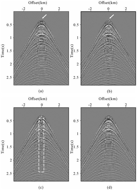
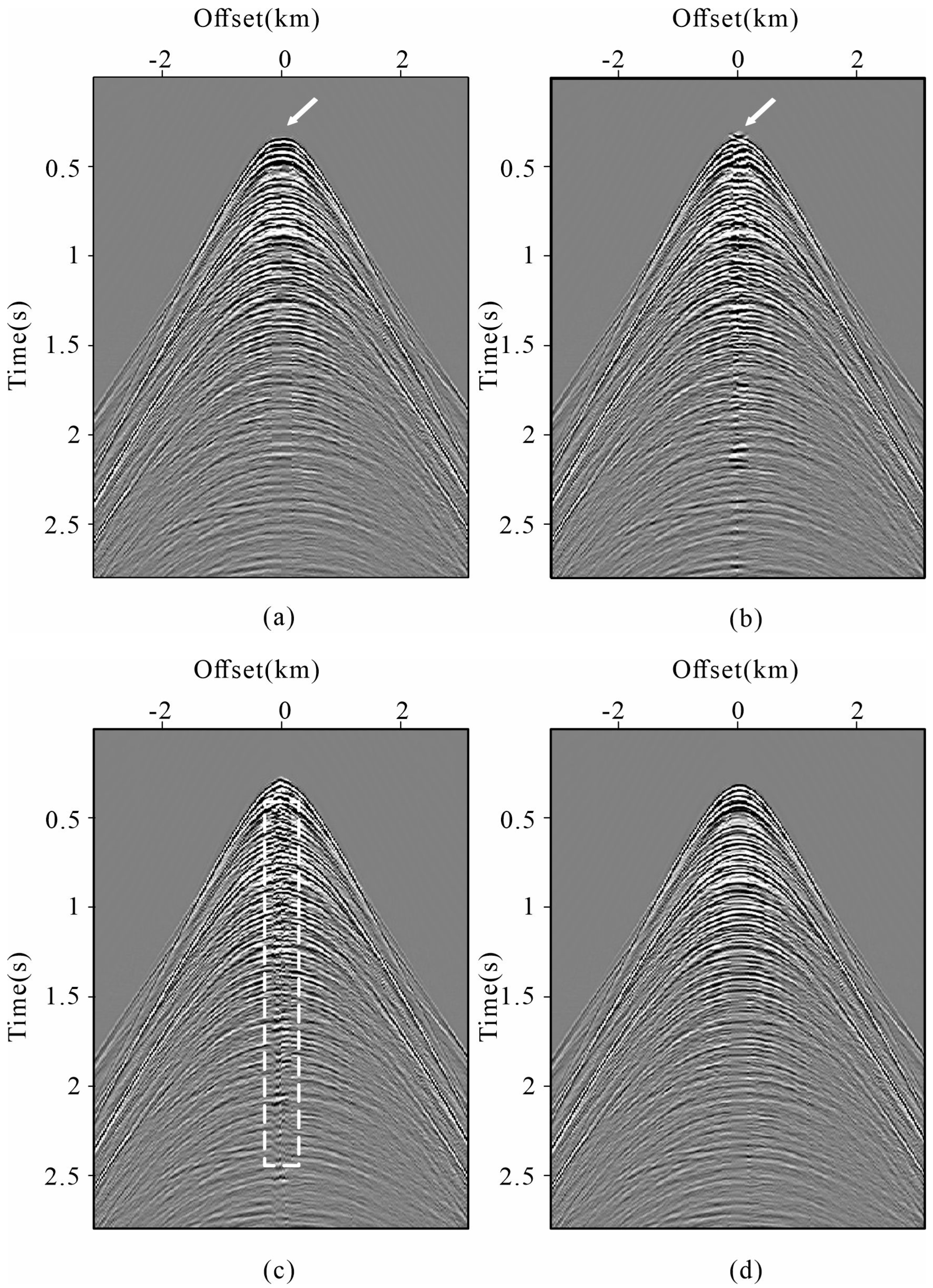
Four reconstruction methods were then applied to the field marine seismic dataset for comparison, as shown in Figure 11. Similar to the results with the synthetic example, we observe that both the radon-based reconstruction method and the curvelet-based reconstruction method exhibit decreased accuracy compared to the interferometric reconstruction methods. Specifically, as shown by the white arrows in Figure 11a,b, the radon-based reconstruction method changed the event curvature in Figure 11a, while the curvelet-based reconstruction method (Figure 11b) caused significant discontinuity in the reconstructed events. In contrast, the interferometric reconstruction methods shown in Figure 11c,d successfully reconstructed the near-offset gap. Yet, it is notable in Figure 11c, as marked by the white dotted box, that some artifacts emerged near the zero offset, leading to a decrease in data quality. Nonetheless, in the proposed method shown in Figure 11d, the reconstructed events exhibit commendable continuity, which proves the effectiveness of the proposed method.

Figure 11. Comparison of the field data reconstruction results: (a) using radon-based reconstruction method; (b) using curvelet-based sparse reconstruction method; (c) using conventional interferometric reconstruction method; (d) using the proposed method.

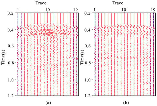
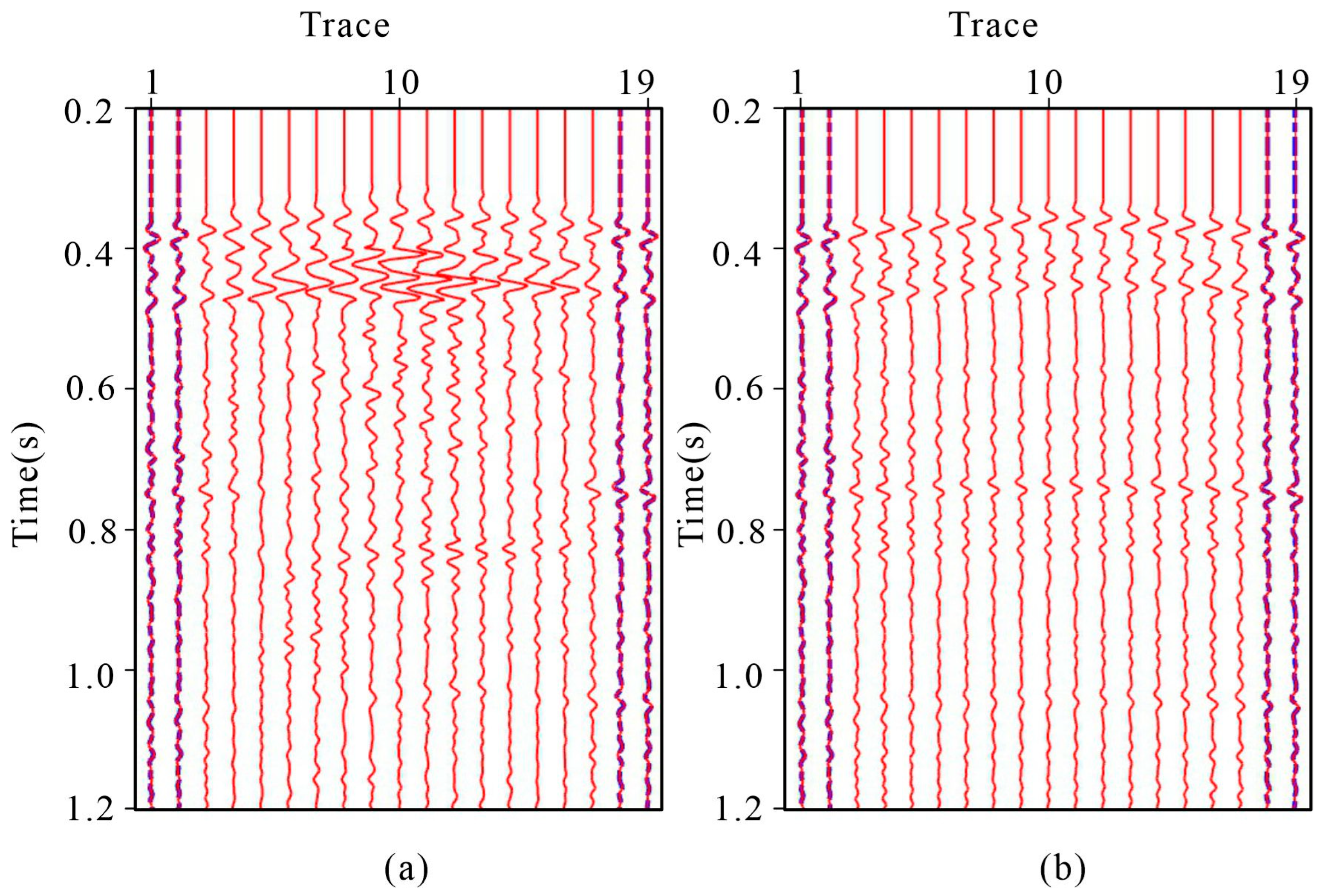
To further examine the local waveform behavior near the acquisition-gap boundary, we compared the reconstructed traces with the nearest available observed traces in Figure 12. It should be emphasized that the adjacent observed trace is not treated as the ground truth of the missing trace. Instead, this comparison is used only to assess waveform continuity and amplitude consistency between the reconstructed region and the neighboring recorded data. The conventional reconstruction shows a more noticeable amplitude mismatch around 0.5 s, whereas the proposed reconstruction exhibits a smoother waveform transition toward the observed data.

Figure 12. Trace-to-trace comparison of the reconstruction results: (a) the reconstructed traces generated by conventional interferometric reconstruction (the red lines) and the original data (the blue lines); (b) the reconstructed traces generated by the proposed method (the red lines) and the original data (the blue lines).

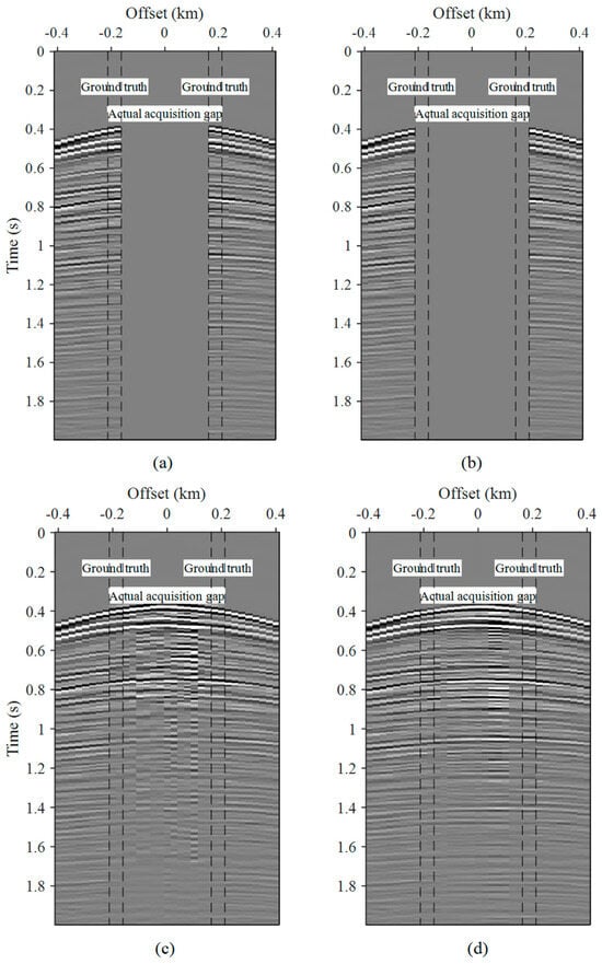
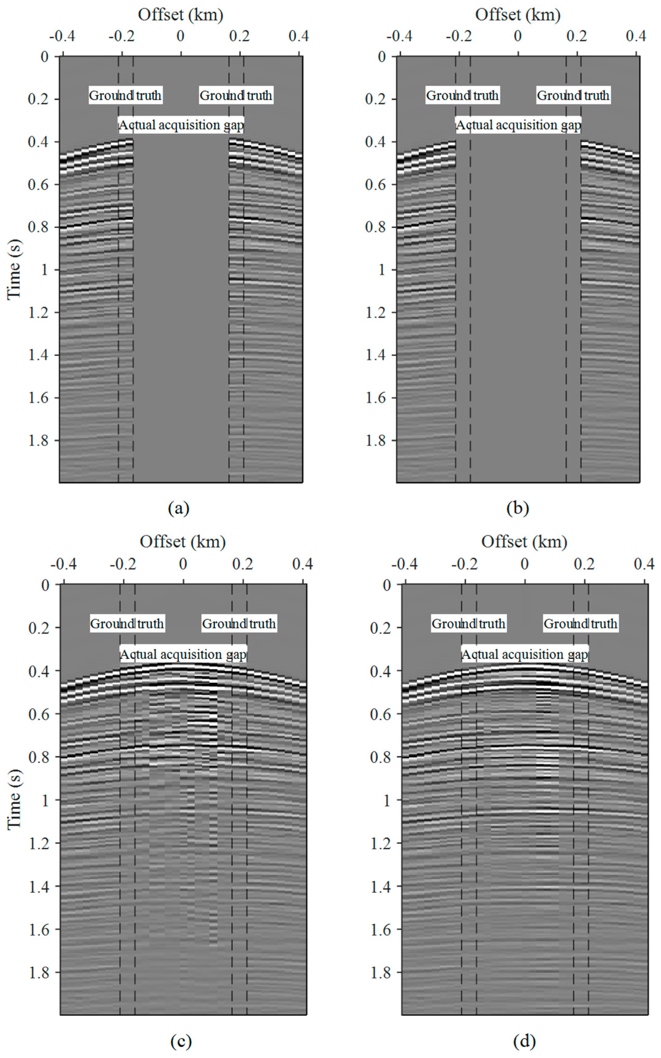
Although Figure 12 illustrates the waveform continuity near the acquisition-gap boundary, the true wavefield inside the actual gap is unavailable and therefore cannot be used for direct accuracy evaluation. To obtain a validation with known ground truth, we further performed a withheld-trace experiment using the recorded field data. Specifically, the validation mask was constructed on the 387 × 387 source–receiver matrix with a spatial interval of 25 m. The actual acquisition gap corresponds to |h| < 175 m. For validation, the two nearest recorded offset classes on each side of the gap, |h| = 175 and 200 m, corresponding to source–receiver lags of 7 and 8, were temporarily withheld and reconstructed, while the original measurements were retained as ground truth. For an N × N source–receiver matrix, each non-zero lag k contains N-k traces for each offset sign. Therefore, the total number of withheld traces is 2 × [(387 − 7) + (387 − 8)] = 1518. The total is slightly smaller than 387 × 4 because the finite acquisition boundaries prevent all shots from contributing traces at both offset signs for both lags.

Figure 13 shows a representative withheld-trace validation result. Both methods recover the artificially removed traces, but the proposed method shows better agreement with the reference data and improved event continuity within the withheld zones. Quantitative evaluation was performed over all 1518 withheld traces (Table 3). The proposed method increases the mean CC from 0.851 to 0.914 and reduces the mean NRMSE from 0.528 to 0.4512, with lower standard deviations for both metrics.

Figure 13. Field-data withheld-trace validation adjacent to the actual near-offset acquisition gap: (a) reference data; (b) input data with artificially withheld traces; (c) conventional interferometric reconstruction; (d) proposed reconstruction.

Table 3. Quantitative evaluation of field-data withheld-trace reconstruction.

Method	Mean_CC	Std_CC	Mean_MSE	Std_MSE	Mean_NRMSE	Std_NRMSE	Ntraces
Conventional	0.851	0.0938	0.0062	0.0045	0.528	0.129	1518
Proposed	0.914	0.0383	0.0043	0.0017	0.4512	0.079	1518

4. Discussion

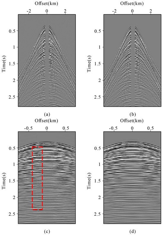
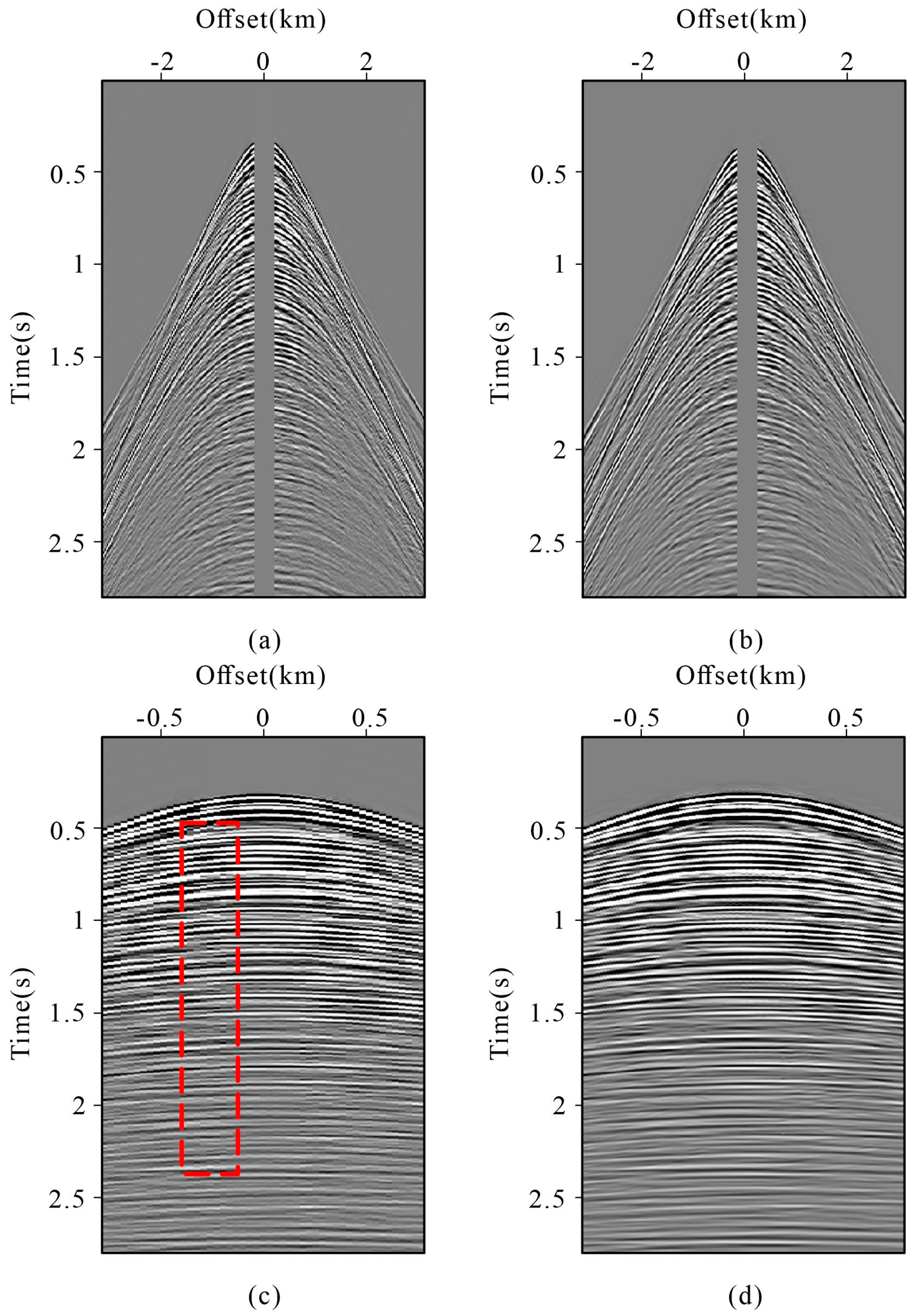
The spatial sampling density can influence interferometric reconstruction because the construction of virtual traces depends on the available source–receiver wavefield. To examine this effect, the field data with an original trace spacing of 25 m were densified to 12.5 m using curvelet-based reconstruction before applying the proposed method. Figure 14c,d compare the near-offset reconstruction results before and after densification. The denser dataset produces improved event continuity in several parts of the reconstructed region. However, because the additional traces are themselves obtained through curvelet-based reconstruction rather than denser physical acquisition, this experiment should be interpreted as an indication that improved spatial sampling can facilitate interferometric reconstruction, rather than as a direct assessment of acquisition-density effects. In practical applications, sufficiently dense and regular spatial sampling is therefore beneficial for the proposed workflow.

Figure 14. Influence of spatial sampling on field-data reconstruction: (a) original data with a 25 m trace spacing; (b) curvelet-densified data with a 12.5 m trace spacing; (c) reconstruction using the original data; (d) reconstruction using the densified data.

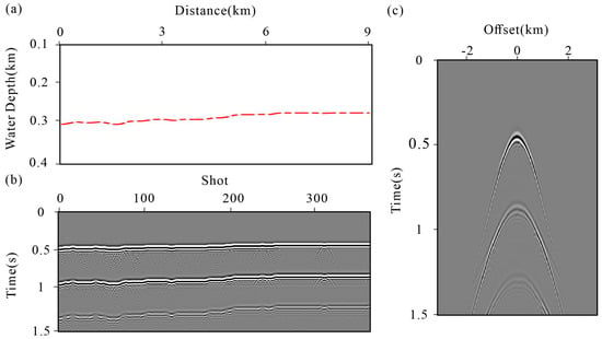
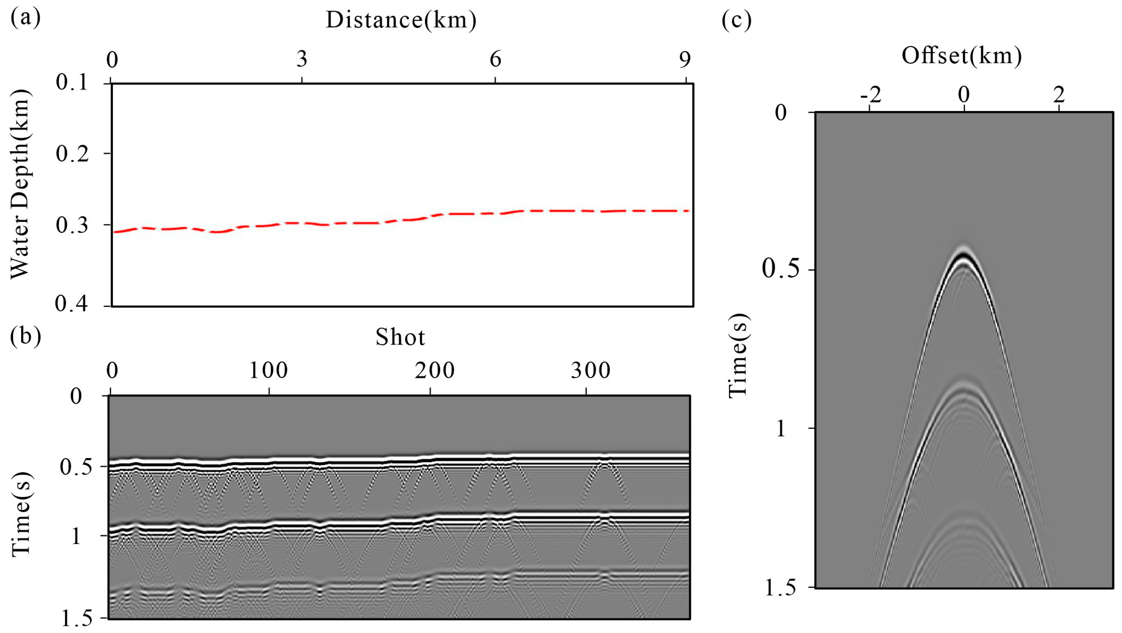
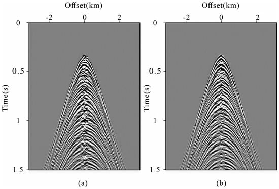
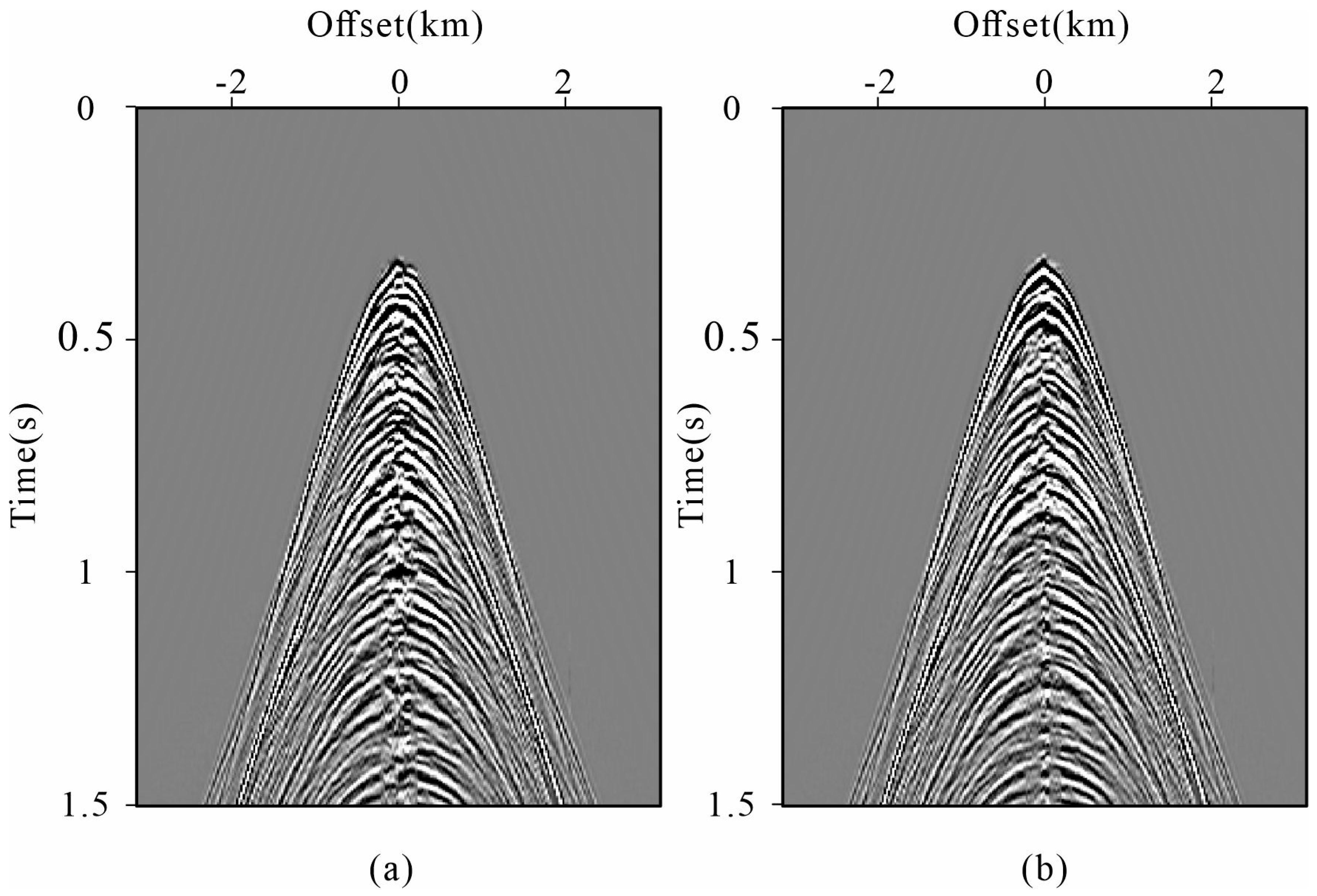
The proposed method requires both the full-wavefield data and an auxiliary primary-wave dataset. In practice, obtaining sufficiently reliable primary data can be difficult, particularly when spatial sampling is incomplete [31]. A possible alternative is to use modeled wavefield information when a sufficiently reliable background model is available [16]. Here, we investigated a simple model-based strategy in which synthetic water-layer-related data are used as the auxiliary input instead of the estimated field primaries. The water-layer model and the corresponding synthetic data are shown in Figure 15. The water-layer model was constructed using a seawater P-wave velocity of 1500 m/s and a density of 1025 kg/m³, while the water-bottom geometry was picked from the stacked seismic section. The corresponding synthetic wavefield was generated using a two-dimensional acoustic finite-difference scheme with second-order temporal and eighth-order spatial accuracy. The spatial grid intervals were 5 m in both horizontal and vertical directions, and the internal modeling time step was 0.5 ms. A 20 Hz Ricker wavelet was used as the source, with source and receiver spacings of 25 m. The modeled data were output at a 4 ms sampling interval. A free-surface boundary was imposed at the top, while 40-grid-point absorbing boundaries were applied along the lateral and bottom edges to suppress artificial boundary reflections.

Figure 15. Demonstration of the data generated using water-layer model within time range of 0–1.5 s: (a) water-layer model; (b) common offset gather; (c) common shot gather.

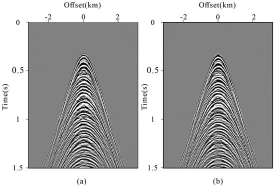
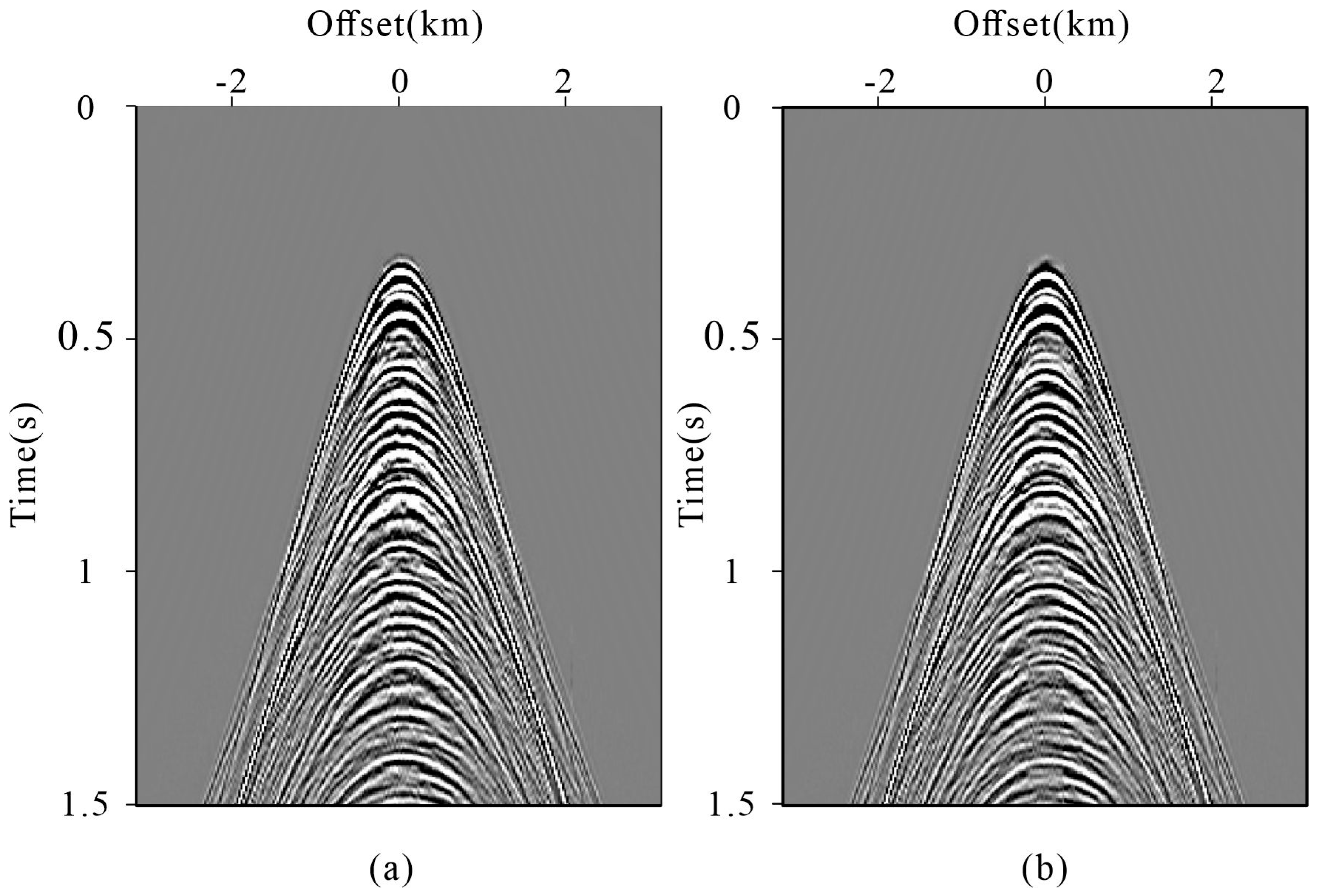
Figure 16 compares the reconstruction after one iteration using the model-based auxiliary data and the field-derived primaries. The model-based result contains stronger shallow artifacts, particularly between approximately 0.3 and 1.0 s, although the principal reconstructed events show comparable continuity. After six iterations (Figure 17), the differences between the two strategies are reduced, and both recover similar major reflection patterns, although local discrepancies remain in the shallow interval. These results suggest that the model-based auxiliary wavefield can serve as a potential alternative when reliable primary-wave estimation is difficult, provided that an adequate background model is available.

Figure 16. Comparison of reconstruction data with single iteration within time range of 0–1.5 s: (a) model-based strategy; (b) control group.

Figure 17. Comparison of final reconstruction result within time range of 0–1.5 s: (a) model-based strategy; (b) control group.

5. Conclusions

In this study, we addressed the reconstruction of near-offset acquisition gaps in marine seismic data using a global amplitude balancing operator (GABO)-enhanced seismic interferometric reconstruction method. By exploiting the focusing characteristics of focal transformation, the proposed GABO enables global amplitude balancing along the offset direction and reduces amplitude inconsistencies and reconstruction artifacts associated with conventional local matching. A projection onto convex sets (POCS)-like iterative framework was further incorporated to progressively refine the reconstructed wavefield and improve reconstruction accuracy. Tests on both synthetic and field marine seismic datasets demonstrated that the proposed method improves near-offset reconstruction in terms of amplitude consistency, artifact suppression, and event continuity. The synthetic tests further showed consistent improvements over different near-offset cutoffs, while the field withheld-trace experiment provided quantitative validation using known measurements.

The results indicate that the proposed method provides an effective approach for recovering missing short-offset information in marine seismic data and has potential for practical marine seismic applications. Nevertheless, its performance remains dependent on the reliability of the auxiliary primary-wave information and the available acquisition geometry. In addition, although the withheld-trace experiment provides direct validation near the acquisition-gap boundary, the reconstructed wavefield inside the actual acquisition gap could not be directly evaluated because no corresponding field measurements are available.

References

- Vermeer, G. Seismic Wavefield Sampling: A Wave Number Approach to Acquisition Fundaments; SEG: Tulsa, OK, USA, 1990. [Google Scholar] [CrossRef] [Scilit]
- Naghizadeh, M.; Sacchi, M.D. Beyond alias hierarchical scale curvelet interpolation of regularly and irregularly sampled seismic data. Geophysics 2010, 75, WB189–WB202. [Google Scholar] [CrossRef] [Scilit]
- Huff, O.R.; Thorkildsen, V.S.; Greiner, T.L.; Lie, J.E.; Evensen, A.K.; Bugge, A.J.; Faleide, J.I. Near offset reconstruction for marine seismic data using a convolutional neural network. Geophys. Prospect. 2024, 72, 2164–2185. [Google Scholar] [CrossRef] [Scilit]
- Widmaier, M.; O’Dowd, D.; Roalkvam, C. Redefining marine towed-streamer acquisition. First Break 2019, 37, 57–62. [Google Scholar] [CrossRef] [Scilit]
- Liu, Y.; Fome, S. Seismic data interpolation beyond aliasing using regularized nonstationary autoregression. Geophysics 2011, 76, V69–V77. [Google Scholar] [CrossRef] [Scilit]
- Gan, S.; Wang, S.; Chen, Y.; Zhang, Y.; Jin, Z. Dealiased Seismic Data Interpolation Using Seislet Transform with Low-Frequency Constraint. IEEE Geosci. Remote Sens. Lett. 2015, 12, 2150–2154. [Google Scholar] [CrossRef] [Scilit]
- Liu, B.; Sacchi, M.D.; Trad, D. Simultaneous interpolation of 4 spatial dimensions. SEG Expand. Abstr. 2004, 23, 2009–2012. [Google Scholar] [CrossRef] [Scilit]
- González, A.S.; Schulte, B.; van der Molen, M.; Oaubel, M.; Dandapani, R.; Detomo, R. Amplitude-Variation-with-Offset Analysis and Interpretation: In Applied Techniques to Integrated Oil and Gas Reservoir Characterization; Elsevier: Amsterdam, The Netherlands, 2021; pp. 301–328. [Google Scholar] [CrossRef] [Scilit]
- Widmaier, M.; Tønnessen, R.; Oukili, J.; Roalkvam, C. Recent advances with wide-tow multi-sources in marine seismic streamer acquisition and imaging. First Break 2020, 38, 75–79. [Google Scholar] [CrossRef] [Scilit]
- Widmaier, M.; Roalkvam, C.; Orji, O. Advanced high-resolution 3D streamer seismic acquisition solutions for new energy applications. In 84th EAGE Annual Conference & Exhibition; European Association of Geoscientists & Engineers: Houten, The Netherlands, 2023; pp. 1–5. [Google Scholar] [CrossRef] [Scilit]
- Joshi, S.; Forjaz, A.; Han, K.S.; Shen, Y.; Queiroga, V.; Selaru, F.A.; Gérard, M.; Xenes, D.; Matelsky, J.; Wester, B.; et al. InterpolAI: Deep learning-based optical flow interpolation and restoration of biomedical images for improved 3D tissue mapping. Nat. Methods 2025, 22, 1556–1567. [Google Scholar] [CrossRef] [Scilit] [PubMed]
- Li, C.; Liu, G.; Hao, Z.; Zu, S.; Mi, F.; Chen, X. Multidimensional Seismic Data Reconstruction Using Frequency-Domain Adaptive Prediction-Error Filter. IEEE Trans. Geosci. Remote Sens. 2018, 56, 2328–2336. [Google Scholar] [CrossRef] [Scilit]
- Yu, S.; Ma, J.; Zhao, B. Off-the-grid vertical seismic profile data regularization by a compressive sensing method. Geophysics 2020, 85, V157–V168. [Google Scholar] [CrossRef] [Scilit]
- Wang, X.; Wang, H.; Zheng, X. High dimensional seismic data interpolation with weighted matching pursuit based on compressed sensing. J. Geophys. Eng. 2014, 11, 0065003. [Google Scholar] [CrossRef] [Scilit]
- Gholami, A. Non-convex compressed sensing with frequency mask for seismic data reconstruction and denoising. Geophys. Prospect. 2014, 62, 1389–1405. [Google Scholar] [CrossRef] [Scilit]
- Trad, D. Interpolation and multiple attenuation with migration operators. Geophysics 2003, 68, 2043–2054. [Google Scholar] [CrossRef] [Scilit]
- Abma, R.; Kabir, N. 3D interpolation of irregular data with a POCS algorithm. Geophysics 2006, 71, E91–E97. [Google Scholar] [CrossRef] [Scilit]
- Wang, Y.; Zhou, H.; Zu, S.; Mao, W.; Chen, Y. Three-Operator Proximal Splitting Scheme for 3-D Seismic Data Reconstruction. IEEE Geosci. Remote Sens. Lett. 2017, 14, 1830–1834. [Google Scholar] [CrossRef] [Scilit]
- Zhou, Z.; Huang, M.; Xu, H.; Yang, X.; Li, Y.; Jia, Z. Deep learning-based interpolation for ground penetrating radar data reconstruction. IEEE J. Sel. Top. Appl. Earth Obs. Remote Sens. 2025, 18, 6329–6335. [Google Scholar] [CrossRef] [Scilit]
- Kaur, H.; Pham, N.; Fomel, S. Seismic data interpolation using deep learning with generative adversarial networks. Geophys. Prospect. 2021, 69, 307–326. [Google Scholar] [CrossRef] [Scilit]
- Saad, O.M.; Fomel, S.; Abma, R.; Chen, Y. Unsupervised deep learning for 3D interpolation of highly incomplete data. Geophysics 2023, 88, WA189–WA200. [Google Scholar] [CrossRef] [Scilit]
- Khoshnavaz, M.J. Oriented extrapolation of common-midpoint gathers in the absence of near-offset data using predictive painting. Geophys. Prospect. 2022, 70, 725–736. [Google Scholar] [CrossRef] [Scilit]
- Wang, B.; Han, D.; Li, J. Missing shots and near-offset reconstruction of marine seismic data with towered streamers via self-supervised deep learning. IEEE Trans. Geosci. Remote Sens. 2022, 60, 1–9. [Google Scholar] [CrossRef] [Scilit]
- Xu, Z.; Sopher, D.; Juhlin, C.; Han, L. Reconstruction of the near-offset gap in marine seismic data using seismic interferometric interpolation. Geophys. Prospect. 2018, 66, 1–26. [Google Scholar] [CrossRef] [Scilit]
- Qiao, B.; Lu, Y.; Li, Q.; Huang, Y.; Liang, S. Data-driven reflection imaging based on seismic interferometry. Geophysics 2022, 87, Q15–Q29. [Google Scholar] [CrossRef] [Scilit]
- Shan, S.; Zhao, F.; Li, Z.; Luo, L.; Li, X. A comprehensive review of optical metrology and perception technologies. Sensors 2025, 25, 6811. [Google Scholar] [CrossRef] [Scilit] [PubMed]
- Huang, Z.; Cao, L. Quantitative phase imaging based on holography: Trends and new perspectives. Light Sci. Appl. 2024, 13, 145. [Google Scholar] [CrossRef] [Scilit] [PubMed]
- Wang, Y.; Luo, Y.; Schuster, G.T. Interferometric interpolation of missing seismic data. Geophysics 2009, 74, SI37–SI45. [Google Scholar] [CrossRef] [Scilit]
- King, S.; Curtis, A. Suppressing nonphysical reflections in Green’s function estimates using source-receiver interferometry. Geophysics 2012, 77, Q15–Q25. [Google Scholar] [CrossRef] [Scilit]
- Wang, Y.; Dong, S.; Luo, Y. Model-based interferometric interpolation method. Geophysics 2010, 75, WB211–WB217. [Google Scholar] [CrossRef] [Scilit]
- Hanafy, S.M.; Schuster, G.T. Interferometric interpolation of sparse marine data. Geophys. Prospect. 2014, 62, 1–16. [Google Scholar] [CrossRef] [Scilit]
- Xu, Z.; Sopher, D.; Juhlin, C.; Han, L.; Gong, X. Radon-domain interferometric interpolation for reconstruction of the near-offset gap in marine seismic data. J. Appl. Geophys. 2018, 151, 125–141. [Google Scholar] [CrossRef] [Scilit]
- Zhou, W.; Butcher, A.; Brisbourne, A.M.; Kufner, S.K.; Kendall, J.M.; Stork, A.L. Seismic noise interferometry and distributed acoustic sensing (DAS): Inverting for the firn layer S-velocity structure on Rutford Ice Stream, Antarctica. J. Geophys. Res. Earth Surf. 2022, 127, e2022JF006917. [Google Scholar] [CrossRef] [Scilit]
- Wang, R.; Hu, B.; Zhang, H.; Zhang, P.; Li, C.; Chen, F. Seismic interferometry for single-channel data: A promising approach for improved offshore wind farm evaluation. Remote Sens. 2025, 17, 325. [Google Scholar] [CrossRef] [Scilit]
- Shirzad, T. High-resolution seismic velocity structure using induced inter-event interferometry at the geothermal sites, Geysers, Eastern California. Geothermics 2024, 116, 102859. [Google Scholar] [CrossRef] [Scilit]
- Stark, H. Image Recovery: Theory and Practice; Academic Press, Inc.: Cambridge, MA, USA, 1978. [Google Scholar]
- Gao, J.; Stanton, A.; Naghizadeh, M.; Sacchi, M.; Chen, X. Convergence improvement and noise attenuation considerations for beyond alias projection onto convex sets reconstruction. Geophys. Prospect. 2013, 61, 138–151. [Google Scholar] [CrossRef] [Scilit]
- Schuster, G.T. Seismic Interferometry; Cambridge University Press: Cambridge, UK, 2009. [Google Scholar]
- Wapenaar, K.; Draganov, D.; Snieder, R.; Campman, X.; Verdel, A. Tutorial on seismic interferometry—Part 1: Basic principles and applications. Geophysics 2010, 75, A195–A209. [Google Scholar] [CrossRef] [Scilit]
- Wapenaar, K. Retrieving the elastodynamic Green’s function of an arbitrary inhomogeneous medium by cross correlation. Phys. Rev. Lett. 2004, 93, 254301. [Google Scholar] [CrossRef] [Scilit] [PubMed]
- Wapenaar, K.; Fokkema, J. Green’s function representations for seismic interferometry. Geophysics 2006, 71, SI33–SI46. [Google Scholar] [CrossRef] [Scilit]
- Wapenaar, K. Green’s function retrieval by crosscorrelation in case of one-sided illumination. Geophys. Res. Lett. 2006, 33, L19340. [Google Scholar] [CrossRef] [Scilit]
- Verschuur, D. Seismic Multiples Removal Technique; EAGE Publications: Houten, The Netherlands, 2006. [Google Scholar]
- Wu, M. Research on optimization of image fast feature point matching algorithm. EURASIP J. Image Video Process. 2018, 2018, 106. [Google Scholar] [CrossRef] [Scilit]
- Berkhout, A.J.; Verschuur, D.J. Focal transformation, an imaging concept for signal restoration and noise removal. Geophysics 2006, 71, A55–A59. [Google Scholar] [CrossRef] [Scilit]
- Hu, B.; Wang, D.; Wang, R. An Iterative Focal Denoising Strategy for Passive Seismic Data. Pure Appl. Geophys. 2020, 177, 4607–4622. [Google Scholar] [CrossRef] [Scilit]
- Yuan, S.; Wang, S.; Luo, C.; Wang, T. Inversion-Based 3-D Seismic Denoising for Exploring Spatial Edges and Spatio-Temporal Signal Redundancy. IEEE Geosci. Remote Sens. Lett. 2018, 15, 1682–1686. [Google Scholar] [CrossRef] [Scilit]
- Verschuur, D.J.; Berkhout, A.J.; Wapenaar, C.P.A. Adaptive surface-related multiple elimination. Geophysics 1992, 57, 1166–1177. [Google Scholar] [CrossRef] [Scilit]
- van Groenestijn, G.J.A.; Verschuur, D.J. Estimating primaries by sparse inversion and application to near-offset data reconstruction. Geophysics 2009, 74, A23–A28. [Google Scholar] [CrossRef] [Scilit]
- Zhang, D.; Verschuur, D.J. Closed-loop surface-related multiple estimation with full-wavefield migration-reconstructed near offsets for shallow water. Geophysics 2021, 86, WC21–WC30. [Google Scholar] [CrossRef] [Scilit]
- Gupta, H.; Kling, H. On typical range, sensitivity, and normalization of Mean Squared Error and Nash-Sutcliffe Efficiency type metrics. Water Resour. Res. 2011, 47, W10601. [Google Scholar] [CrossRef] [Scilit]
- Asuero, A.G.; Sayago, A.; González, A.G. The correlation coefficient: An overview. Crit. Rev. Anal. Chem. 2006, 36, 41–59. [Google Scholar] [CrossRef] [Scilit]
- Ibrahim, A.; Terenghi, P.; Sacchi, M. Simultaneous reconstruction of seismic reflections and diffractions using a global hyperbolic Radon dictionary. Geophysics 2018, 83, V315–V323. [Google Scholar] [CrossRef] [Scilit]
- Lin, T.; Si, Q. Reconstruction of seismic data based on SFISTA and curvelet transform. Front. Earth Sci. 2023, 11, 1176435. [Google Scholar] [CrossRef] [Scilit]
Disclaimer/Publisher’s Note: The statements, opinions and data contained in all publications are solely those of the individual author(s) and contributor(s) and not of MDPI and/or the editor(s). MDPI and/or the editor(s) disclaim responsibility for any injury to people or property resulting from any ideas, methods, instructions or products referred to in the content. |
© 2026 by the authors. Licensee MDPI, Basel, Switzerland. This article is an open access article distributed under the terms and conditions of the Creative Commons Attribution (CC BY) license.