


Abstract
Automatic Identification System (AIS) data are widely used for maritime traffic analysis, vessel monitoring, and intelligent navigation systems. However, missing trajectory segments caused by irregular reporting intervals and communication disruptions can degrade the continuity and reliability of vessel trajectories. This study proposes a vessel-condition-aware AIS trajectory restoration framework that combines Cubic Spline-based preliminary restoration with a Feature-wise Linear Modulation (FiLM)-conditioned Transformer and gated bounded residual correction. For AIS sequences of 200 points, the central 60 points are treated as missing segments, and Cubic Spline interpolation is first applied to generate a preliminary trajectory. The proposed model then predicts residual corrections by incorporating vessel-specific condition information, including hull geometry features, maneuvering-related descriptors, and appendage-related proxy descriptors, into Transformer representations through FiLM modulation. Experimental results show that the proposed method reduces the average Euclidean distance (AED) from 145.43 m to 134.20 m and the maximum displacement error (MDE) from 286.03 m to 269.45 m compared with Cubic Spline interpolation, corresponding to improvements of 7.73% and 5.80%, respectively. The proposed method also achieves lower AED than recurrent residual correction models, including BiLSTM. Condition-shuffling analysis further demonstrates that vessel-specific condition information contributes to improved AIS trajectory restoration performance.
1. Introduction
The Automatic Identification System (AIS) is a maritime communication system that periodically transmits and receives information such as vessel position, speed, course, heading, and time. AIS data have been widely used in various maritime applications, including maritime traffic analysis, vessel traffic monitoring, and port operations. The spatiotemporal movement characteristics and navigation patterns of vessels can be analyzed using AIS data, enabling a wide range of applications such as route inference, abnormal behavior detection, collision risk assessment, and decision support for vessel operations [1,2,3]. In particular, with the recent development of autonomous ships and intelligent maritime traffic management systems, data-driven modeling based on large-scale vessel operation data has become increasingly important, and the availability of reliable AIS trajectory data is one of the key factors affecting the performance of such technologies.
However, AIS data collected in actual operating environments are not always recorded continuously and accurately. Missing data and abnormal observations may occur because of equipment and antenna installation conditions, signal reception environments, uncertainties in message transmission and reception, and human errors [4,5]. Consequently, real-world AIS datasets may contain missing values, outliers, irregular sampling intervals, and abnormal positional changes, which can degrade the continuity and reliability of vessel trajectories. In particular, when vessel position information is consecutively unavailable for a certain period, the missing path must be reconstructed using only the observations available before and after the missing segment. Therefore, an effective restoration method should consider both the overall continuity of the trajectory and the motion characteristics of the vessel.
Missing AIS trajectory information can also have practical and economic consequences in maritime operations. In port and coastal waters with dense vessel traffic, incomplete trajectories may reduce the reliability of traffic monitoring and collision-risk assessment, potentially affecting navigational safety and the efficiency of vessel traffic management. Reliable trajectory restoration can reduce uncertainty in vessel movement analysis and support safer and more efficient port operations, traffic management, and post-event investigation. In addition, continuous vessel movement information is important for maritime surveillance applications, including the detection of suspicious or illegal fishing activities and the monitoring of vessels of interest. Therefore, improving the continuity of AIS trajectories can enhance maritime situational awareness and support decision-making in port management, maritime law enforcement, and maritime security applications [2,3].
Various approaches have been investigated to improve the quality of AIS trajectories, ranging from mathematical interpolation methods such as linear interpolation, Cubic Spline interpolation, and Hermite interpolation to trajectory reconstruction methods that incorporate vessel navigation states and kinematic characteristics [6,7,8]. Studies have also addressed the detection and correction of anomalous AIS observations and the restoration of sparse vessel trajectories [9,10,11]. More recently, the scope of AIS trajectory reconstruction has expanded toward data-driven reconstruction and imputation approaches that exploit historical trajectory patterns, structural similarities among trajectories, and generative models [12,13,14,15].
Meanwhile, the nonlinear temporal modeling capability of neural networks has been increasingly applied to AIS trajectory modeling. RNN-, LSTM-, and Seq2Seq-based models have been used to learn temporal dependencies in AIS sequences [16,17], and methods incorporating multiple types of trajectory information, including position, speed, course, traveled distance, and vessel type, have also been proposed [18]. More recently, Transformer-based approaches have been introduced into AIS trajectory modeling because self-attention enables direct modeling of relationships between temporally distant observations within a sequence [19,20].
However, most existing RNN- and Transformer-based AIS studies have primarily focused on trajectory prediction, in which future vessel positions are estimated from past observations. In trajectory prediction, unobserved future trajectories must be generated using only historical information. In contrast, trajectory restoration aims to reconstruct a missing intermediate segment by exploiting observations available both before and after the missing interval. Therefore, trajectory restoration requires a model capable of simultaneously utilizing bidirectional contextual information while preserving the overall trajectory shape and recovering local motion variations within the missing segment.
In addition, most AIS-based trajectory models primarily rely on dynamic navigation variables such as latitude, longitude, speed, and course. However, the actual motion response of a vessel is influenced not only by its current navigation state but also by its length, breadth, draft, hull-form ratios, and maneuvering characteristics. Even under similar speeds and course changes, vessels with different sizes and geometries may exhibit different turning responses and lateral motion characteristics [21]. Yang et al. demonstrated the potential of vessel-specific information by incorporating vessel attributes such as length, breadth, draft, and vessel type into a trajectory prediction model [22]. However, directly concatenating vessel particulars with dynamic AIS variables may not sufficiently represent the relative physical meaning of individual vessel characteristics, while the roles of static vessel-condition information and dynamic temporal information may also remain insufficiently separated within the model.
In the field of ship maneuvering, various dimensionless variables and hydrodynamic coefficients have been used to describe vessel geometry and maneuvering-related characteristics. The MMG-based maneuvering model represents surge, sway, and yaw motions by separately considering the effects of the hull, propeller, and rudder, and vessel particulars such as length, breadth, draft, block coefficient, and propeller- and rudder-related characteristics are closely associated with vessel motion responses [21]. However, it is generally impractical to obtain accurate hydrodynamic derivatives, maneuvering trial results, and detailed appendage specifications for every vessel contained in large-scale AIS datasets. Therefore, rather than directly applying a complete physics-based maneuvering model to AIS trajectory restoration, a practical alternative is to construct condition variables from available vessel particulars to represent vessel-specific differences in geometry and maneuvering-related characteristics and incorporate them into a data-driven model.
Another important issue is how heterogeneous types of information are incorporated into the learning architecture. Simply concatenating different types of inputs into a single feature vector makes it difficult to explicitly control how condition information affects temporal feature representations. Feature-wise Linear Modulation (FiLM) is a conditional learning approach in which feature-wise scaling and shifting parameters are generated from external condition information and applied to hidden representations within a neural network [23]. By using FiLM, vessel-specific condition information can modulate the internal representations of a Transformer rather than being directly concatenated with the AIS sequence. This structure enables the model to form different internal representations for similar AIS motion patterns according to vessel-specific conditions, making it potentially suitable for trajectory restoration that accounts for differences among vessels.
In this study, we propose a Transformer-based AIS trajectory restoration method that incorporates vessel particulars and maneuvering-related condition information. First, Cubic Spline interpolation is applied to the missing segment to obtain a preliminary trajectory that captures the overall trend of vessel motion. Rather than regenerating the entire trajectory, the Transformer estimates the residual error of this preliminary restoration. Dynamic AIS information and vessel-specific condition information are processed through separate branches. The condition features consist of dimensionless geometric variables, AIS-based motion and maneuvering-related descriptors, and appendage-related proxy descriptors. The Transformer serves as the main sequence modeling backbone, while FiLM acts as a conditioning mechanism that modulates the Transformer hidden representations according to vessel-specific information. In addition, a gated bounded residual correction mechanism is introduced to prevent excessive modification of the preliminary trajectory.
The methodological contribution of this study does not lie in the independent introduction of Cubic Spline interpolation, Transformer self-attention, or FiLM. Rather, it lies in integrating these components into a vessel-condition-aware residual restoration framework specifically designed for intermediate AIS trajectory gaps. In particular, vessel-specific condition information is incorporated through FiLM-based modulation, while the Transformer predicts a bounded residual correction with respect to a stable Cubic Spline preliminary trajectory instead of reconstructing the missing trajectory entirely from scratch.
2. Literature Review
2.1. AIS Trajectory Interpolation and Restoration
Various trajectory interpolation and restoration methods have been investigated to address missing observations, outliers, and sparsity in AIS data. Early studies mainly employed mathematical interpolation techniques, such as linear interpolation, Cubic Spline interpolation, and Hermite interpolation, to continuously connect missing vessel positions. Nguyen et al. proposed an interpolation method for missing AIS data to improve the continuity of AIS state information, including position, speed, course, and heading [6]. Zaman et al. proposed an interpolation-based approach for inferring trajectory waypoints from limited observations in sparse AIS data [10]. These interpolation-based approaches are relatively simple to implement and can provide a stable overall trajectory shape by connecting the observations available before and after a missing segment.
In addition to direct interpolation of missing positions, trajectory reconstruction methods that account for vessel navigation states and abnormal trajectories have also been investigated to improve the quality of AIS trajectories. Zhang et al. proposed a multi-regime trajectory reconstruction approach in which abnormal observations in raw AIS data were first removed, after which vessel navigation states were classified into hoteling, maneuvering, and normal-speed sailing for state-specific trajectory fitting [7]. The study also employed an AIS quality assessment metric considering vessel maneuverability constraints. These results indicate that AIS trajectory reconstruction should account not only for the geometric continuity of coordinates but also for vessel navigation states and motion characteristics.
Guo et al. proposed an improved kinematic interpolation method for AIS trajectory reconstruction that incorporates kinematic information such as vessel speed and acceleration [8]. Compared with conventional position-based interpolation, this approach attempts to construct physically more plausible trajectories by considering vessel motion states. However, interpolation and kinematic reconstruction methods generally depend on the available observations and predefined mathematical relationships. Therefore, they may have limited ability to represent complex nonlinear trajectory variations when long missing intervals, significant turning motions, or substantial speed changes occur. In contrast, the proposed method does not use kinematic variables as direct interpolation constraints, but instead incorporates vessel-specific geometry and maneuvering characteristics as conditioning information to modulate a Transformer-based residual correction model.
Studies have also focused on detecting and correcting abnormal observations in raw AIS trajectories to improve trajectory reliability. Yan et al. proposed an integrated framework that detects trajectory glitches using statistical theory and a sliding window, rectifies the detected abnormal observations using linear interpolation, and subsequently performs trajectory compression [9]. Although this study primarily addressed noise detection, rectification, and compression rather than long-term missing trajectory restoration, it demonstrates the importance of detecting and correcting abnormal positions when constructing reliable AIS trajectories.
More recently, neural networks have been employed to restore missing segments of AIS trajectories by exploiting their nonlinear learning capability. Xue performed AIS trajectory restoration using a radial basis function (RBF) neural network and applied fractional-order gradient descent with momentum to improve training performance [24]. Ye et al. proposed a multi-step restoration method for sparse vessel trajectories by combining Cubic Spline-based preliminary restoration with Seq2Seq-based secondary restoration [11]. This method is meaningful in that it combines the stable initial trajectory provided by Cubic Spline interpolation with the nonlinear temporal learning capability of a neural network. However, the restoration model mainly focuses on correlations among AIS features and does not explicitly incorporate vessel-specific particulars or maneuvering-related characteristics as conditioning information.
Beyond the spatiotemporal information contained within an individual trajectory, recent studies have also exploited historical trajectory patterns and structural relationships among multiple trajectories. Liang et al. proposed AISClean, a framework for trajectory reconstruction under uncertain AIS conditions [12]. AISClean detects noise and missing observations using statistical methods and subsequently combines Geohash and Dynamic Time Warping to reconstruct damaged trajectories based on historical trajectory information. Wu et al. proposed the Customized Tensor-Based Maritime Trajectory Reconstruction (CTMTR) framework, which exploits self-similarity among vessel trajectories and applies low-rank tensor completion to reconstruct trajectories in the presence of missing and abnormal AIS data [13].
Generative modeling approaches have also recently been introduced for trajectory imputation. Wang et al. proposed TrajDiff, which applies a resampled conditional diffusion model to vessel trajectory imputation from a generative modeling perspective [14]. Spiliopoulos et al. proposed HABIT, an H3 aggregation-based imputation framework that utilizes historical AIS movement patterns to restore missing vessel mobility data at scale [15].
Overall, previous AIS trajectory restoration studies have progressed from geometric interpolation toward kinematic reconstruction that incorporates vessel motion states, and more recently toward data-driven imputation and reconstruction using neural networks, historical trajectory patterns, trajectory self-similarity, and generative modeling. However, these approaches primarily rely on the observed AIS sequence itself or on surrounding and historical trajectory patterns. Kinematic reconstruction methods additionally use motion-state variables such as speed and acceleration to constrain or interpolate missing positions, but they generally do not explicitly account for vessel-specific differences in geometry and maneuvering characteristics.
In AIS trajectory restoration, the observations before and after a missing segment already provide information about the overall path continuity, whereas the detailed motion within the missing interval may vary depending on vessel-specific characteristics. Therefore, this study constructs vessel-geometry features and maneuvering-related descriptors from vessel particulars and AIS-derived motion information and uses them as conditioning information rather than as direct interpolation constraints. Specifically, Cubic Spline interpolation first provides a preliminary trajectory representing the overall trajectory trend, while FiLM modulates the Transformer hidden representations according to vessel-specific conditions. The conditioned Transformer then predicts residual corrections to refine the preliminary trajectory. This approach enables vessel-specific information to influence the restoration of local trajectory variations within the missing segment.
2.2. Deep Learning-Based Vessel Trajectory Modeling
AIS trajectories are sequential data in which vessel positions and navigation states vary over time. Accordingly, recurrent neural network-based methods such as RNNs, LSTMs, and Seq2Seq models have been widely applied to vessel trajectory modeling. Capobianco et al. proposed an encoder–decoder RNN-based Seq2Seq model for predicting future vessel trajectories from historical AIS observations [16]. Their study demonstrated the potential of data-driven trajectory prediction by learning temporal dependencies within AIS sequences. Murray and Perera also developed an AIS-based deep learning framework for regional ship behavior prediction and showed that regional vessel movement characteristics can be learned from historical AIS time series [25].
Studies have also investigated the use of multiple navigation variables in addition to vessel position for trajectory prediction. Li et al. compared and analyzed various machine learning- and deep learning-based AIS trajectory prediction models, emphasizing the importance of effectively representing dynamic vessel navigation information in trajectory modeling [17]. Zhang et al. proposed METO-S2S, in which coordinate, speed, course, and sailing distance are processed using a Multiple-semantic Encoder, while vessel type and departure time are used as guidance information in a Type-Oriented Decoder [18]. This approach demonstrates that vessel- and voyage-related auxiliary information, in addition to dynamic AIS variables, can be incorporated into trajectory modeling.
However, RNN- and LSTM-based models process input sequences sequentially, which may limit their ability to efficiently represent relationships between temporally distant observations in long AIS sequences. To overcome this limitation, Transformer-based AIS trajectory models using self-attention have recently been investigated. Jiang et al. proposed TRFM-LS and applied a Transformer-based deep learning architecture to vessel trajectory prediction [19]. Nguyen and Fablet proposed TrAISformer, which combines a sparse augmented data representation with cross-entropy loss to perform long-term vessel trajectory prediction while accounting for the heterogeneous and multimodal characteristics of AIS trajectories [20]. These studies demonstrate that Transformers can effectively model long-term temporal dependencies and complex movement patterns in AIS sequences.
Nevertheless, a substantial proportion of existing deep learning-based AIS studies focus on trajectory prediction, in which future vessel positions are estimated from previously observed AIS sequences. In trajectory prediction, observations after the target prediction time are unavailable, and the model must therefore generate future vessel positions using only historical navigation information. In contrast, trajectory restoration is performed when observations are available both before and after a missing segment, allowing the model to exploit contextual information from both directions. In particular, when a continuous intermediate segment is missing, it is important to simultaneously consider the navigation states before the missing segment and the observations after it in order to preserve the overall trajectory shape.
Therefore, rather than directly applying conventional trajectory prediction models to the restoration problem, the model architecture should reflect the different information structure of trajectory restoration. Interpolation methods such as Cubic Spline can provide a stable preliminary trajectory by using observations before and after the missing segment. A neural network can then be designed to correct only the local errors of this initial restoration rather than regenerating the entire trajectory from scratch. In the present study, the temporal representation capability of Transformer self-attention is utilized while the model is designed to perform residual correction on the Cubic Spline preliminary trajectory. This formulation distinguishes the proposed approach from conventional future trajectory prediction models.
2.3. Vessel Characteristics, Maneuverability, and Conditional Modeling
Most AIS-based trajectory models use dynamic navigation information such as latitude, longitude, speed over ground (SOG), course over ground (COG), and heading as their primary inputs. However, the actual motion response of a vessel is influenced not only by its current navigation state but also by vessel-specific characteristics such as length, breadth, draft, hull-form ratios, and maneuvering characteristics. For example, even under similar speeds and course changes, vessels with different sizes and hull geometries may exhibit different turning radii, lateral motions, and yaw responses [21]. Therefore, incorporating vessel particulars and geometric characteristics into a trajectory model can potentially improve the restoration of motion variations within missing segments in a vessel-specific manner.
Recent trajectory prediction studies have begun to incorporate vessel-specific information into AIS trajectory modeling. Zhang et al. used vessel type and departure time as guidance information in the decoder of METO-S2S to account for differences in vessel and voyage conditions during trajectory prediction [18]. Yang et al. proposed VEPO-S2S, which uses a vessel portrait including vessel length, breadth, draft, and vessel type to perform vessel-specific trajectory prediction [22]. These studies indicate that incorporating vessel-specific information in addition to AIS time-series data can be beneficial for vessel trajectory modeling.
However, directly concatenating the absolute values of vessel particulars with dynamic AIS variables may not adequately represent the relative physical significance of these parameters for vessels of different sizes. Furthermore, when dynamic navigation information and static vessel characteristics are processed as a single input feature vector, it may be difficult to distinguish how each type of information affects the temporal hidden representation. For the trajectory restoration problem considered in this study, a condition representation that captures relative differences in vessel size, geometry, and motion response is more informative than simply providing vessel identification or unprocessed vessel particulars.
In the field of ship maneuvering, various dimensionless variables and maneuvering-related coefficients have been used to describe vessel motion responses. Yasukawa and Yoshimura summarized the MMG standard method, which predicts surge, sway, and yaw motions by separately representing the effects of the hull, propeller, and rudder [21]. In the MMG framework, vessel length, breadth, draft, block coefficient, and appendage-related characteristics are important factors associated with lateral motion and turning response.
However, obtaining accurate hydrodynamic derivatives, maneuvering trial results, and detailed propeller and rudder specifications for every vessel in a large-scale AIS dataset is generally impractical. Therefore, the present study does not directly apply the complete MMG maneuvering equations to AIS trajectory restoration. Instead, vessel geometry- and maneuvering-related descriptors are constructed using available vessel particulars and AIS-derived motion information. In addition, because propeller- and rudder-related information is generally unavailable in AIS datasets, the relative principal-dimension relationships of the KRISO Container Ship (KCS) reference hull are used to construct proxy descriptors that represent relative appendage-related characteristics according to vessel size, rather than to estimate the actual appendage dimensions of individual vessels.
Another important consideration is how such condition information should be incorporated into a neural network. Feature-wise Linear Modulation (FiLM), proposed by Perez et al., is a conditional modulation approach in which feature-wise scaling and shifting parameters are generated from external condition information and applied to the hidden representations of a neural network [23]. Rather than simply adding the condition variables to the original input features, FiLM directly modifies the intermediate feature representations learned by the model according to the given conditions.
In this study, the FiLM conditional modulation concept is applied to AIS trajectory restoration. Dynamic AIS information and vessel-specific condition information are processed through separate branches, and FiLM parameters generated from dimensionless vessel geometry features, AIS-based motion and maneuvering-related descriptors, and appendage-related proxy descriptors are applied to the hidden representations of the Transformer blocks. This enables the model to learn different temporal representations for identical or similar AIS motion patterns according to vessel-specific size, geometry, and maneuvering-related conditions. Unlike simple feature concatenation, the proposed structure allows vessel condition information to directly modulate the hidden representations used in the trajectory restoration process.
3. Problem Description and Methodology
3.1. Data Description
In this study, real-world AIS data collected in the waters near Ulsan Port were used to formulate the missing trajectory restoration problem. The AIS dataset contains dynamic navigation information, including the Maritime Mobile Service Identity (MMSI), timestamp, latitude, longitude, speed over ground (SOG), course over ground (COG), and heading. In addition, vessel particulars such as vessel length, breadth, draft, and gross tonnage were incorporated to construct vessel-specific condition information.
The study area was restricted to 35.3823296–35.5412299° N latitude and 129.3500011–129.5073977° E longitude. Records with invalid geographic coordinates, SOG values outside the range of 0–50 knots, or COG values outside 0–360° were removed. Heading values outside 0–360° were treated as invalid and replaced by the corresponding COG values when available. Records with missing essential variables, including MMSI, latitude, longitude, timestamp, SOG, COG, vessel length, breadth, or draft, were excluded. Vessel-particular records were retained only when the vessel length was between 0 and 500 m, breadth between 0 and 100 m, and draft between 0 and 30 m. The remaining records were sorted by MMSI and timestamp, and consecutive records were divided into separate trajectory segments when the time interval between adjacent observations exceeded 1000 s or was non-positive. Only trajectory segments containing at least 200 AIS points were retained. Finally, segments in which the maximum inter-point speed, calculated from the geographic distance and time interval between consecutive AIS positions, exceeded 60 knots were removed.
The AIS data used in this study were collected in the waters near Ulsan Port from 6 August to 31 August, 2020, within a spatial boundary of 35.3823296–35.5412299° N latitude and 129.3500011–129.5073977° E longitude. After initial preprocessing, 1,226,791 AIS records from 776 unique MMSIs remained. Subsequent trajectory segmentation and quality filtering resulted in a total of 1902 valid trajectory segments comprising 648,250 AIS points. A trajectory-wise data split was then applied, resulting in 1331 trajectories for training, 285 trajectories for validation, and 286 trajectories for testing. Fixed-length windows were subsequently generated from these trajectory segments, yielding 4369 training samples, 1010 validation samples, and 988 test samples. The resulting sequences were used for subsequent missing-segment generation, Cubic Spline-based preliminary restoration, and training of the FiLM-conditioned Transformer model. The data used in this study are available upon reasonable request.
The spatial distribution of the preprocessed AIS records is shown in Figure 1. As illustrated in the figure, AIS points are densely distributed within the inner waters of Ulsan Port and along the major port approach routes, and the principal vessel traffic patterns within the study area are clearly identifiable. This spatial distribution indicates that the dataset used in this study captures representative vessel traffic characteristics in the waters near Ulsan Port.
Figure 1.
Spatial distribution of preprocessed AIS records in the study area near Ulsan port.
3.2. Problem Description
In this study, we consider an AIS trajectory restoration problem in which a continuous missing segment occurs within an AIS trajectory sequence of a fixed length. The objective is to reconstruct the missing vessel positions using the observations available before and after the missing segment. Each trajectory sample is defined as a time series of length (T), and the complete AIS feature sequence of the (i)-th sample is expressed as Equation (1).
where the corresponding variable denotes the AIS feature vector of the (i)-th sample at time step (t). In this study, the AIS feature vector includes latitude, longitude, speed, course, heading, time interval, and change-related features derived from these variables. The direct target of trajectory restoration is the vessel position at each time step, which is defined in Equation (2).
To formulate the missing trajectory restoration problem, the complete set of time steps is divided into an observed set and a missing set. The observed and missing time-step sets are mutually exclusive and together constitute the complete sequence. This relationship is expressed in Equation (3).
For model training and evaluation, a continuous missing segment is artificially generated by masking the central portion of each original AIS trajectory. The total sequence length is set to (T = 200), and the central 30%, corresponding to (M = 60) consecutive AIS points, is treated as the missing segment. The binary mask variable indicating whether each time step belongs to the missing region is defined in Equation (4).
where () indicates that time step (t) of the (i)-th sample belongs to the missing region to be restored, whereas () indicates that the corresponding time step belongs to the observed region () and is used as contextual information by the model. During training, the original AIS position is retained as the ground truth. However, the actual position information corresponding to the missing region () is assumed to be unavailable to the model input.
For the missing interval, the original position coordinates are not directly provided to either the AIS branch or the condition branch. Instead, a preliminary sequence is first constructed using Cubic Spline interpolation. The dynamic variables used at the masked time steps are represented by the corresponding preliminary reconstructed values, and change-related features are subsequently recalculated from this reconstructed sequence. Consequently, the ground-truth positions within the missing interval are retained only as target values for training and performance evaluation, rather than being directly used to construct the position-derived condition features. Thus, the masked interval does not retain the original SOG, COG, heading, or position values as direct dynamic inputs; instead, the corresponding preliminary reconstructed values are used to form the model input sequence. The timestamp information is retained only to preserve the temporal spacing of the artificially masked sequence, and the corresponding time-interval features are used as temporal coordinates rather than as vessel-state observations.
To provide an intuitive illustration of the restoration problem, Figure 2 presents a representative AIS trajectory sample used in this study. The trajectory consists of 200 consecutive AIS observations and is divided into two observed context regions and one central missing region. The 60 consecutive points located in the central 30% of the sequence are artificially masked, whereas the observations before and after the missing interval remain available to the restoration model. For visualization purposes, the original trajectory within the masked region is shown as the ground truth; however, these position values are not provided as model inputs during training or evaluation. The objective of the restoration model is to reconstruct this unobserved intermediate path using the contextual information available on both sides of the missing interval while maintaining positional and directional continuity at the boundaries.
To represent this setting, the model input sequence after preliminary reconstruction is denoted by . In the observed region, retains the original AIS feature vectors, whereas in the missing region, the corresponding dynamic variables are represented using the preliminary reconstructed values. The resulting input sequence is defined as Equation (5).
where denotes the input feature vector constructed using the preliminary reconstructed values within the missing region, while the original ground-truth position values in are not provided to the model.
Accordingly, the model estimates the vessel positions within the missing region () using the masked input sequence () and the corresponding mask sequence (). The objective of AIS trajectory restoration is to estimate the restored positions () such that they are close to the ground-truth positions () for (). This restoration problem can be expressed in a general functional form as Equation (6).
where () denotes the trainable trajectory restoration model, and () denotes the set of restored vessel positions within the missing region. In other words, the model reconstructs the missing vessel positions by exploiting the observations available before and after the missing segment together with the corresponding mask information.
Figure 2.
Representative AIS trajectory showing observed and missing segments.
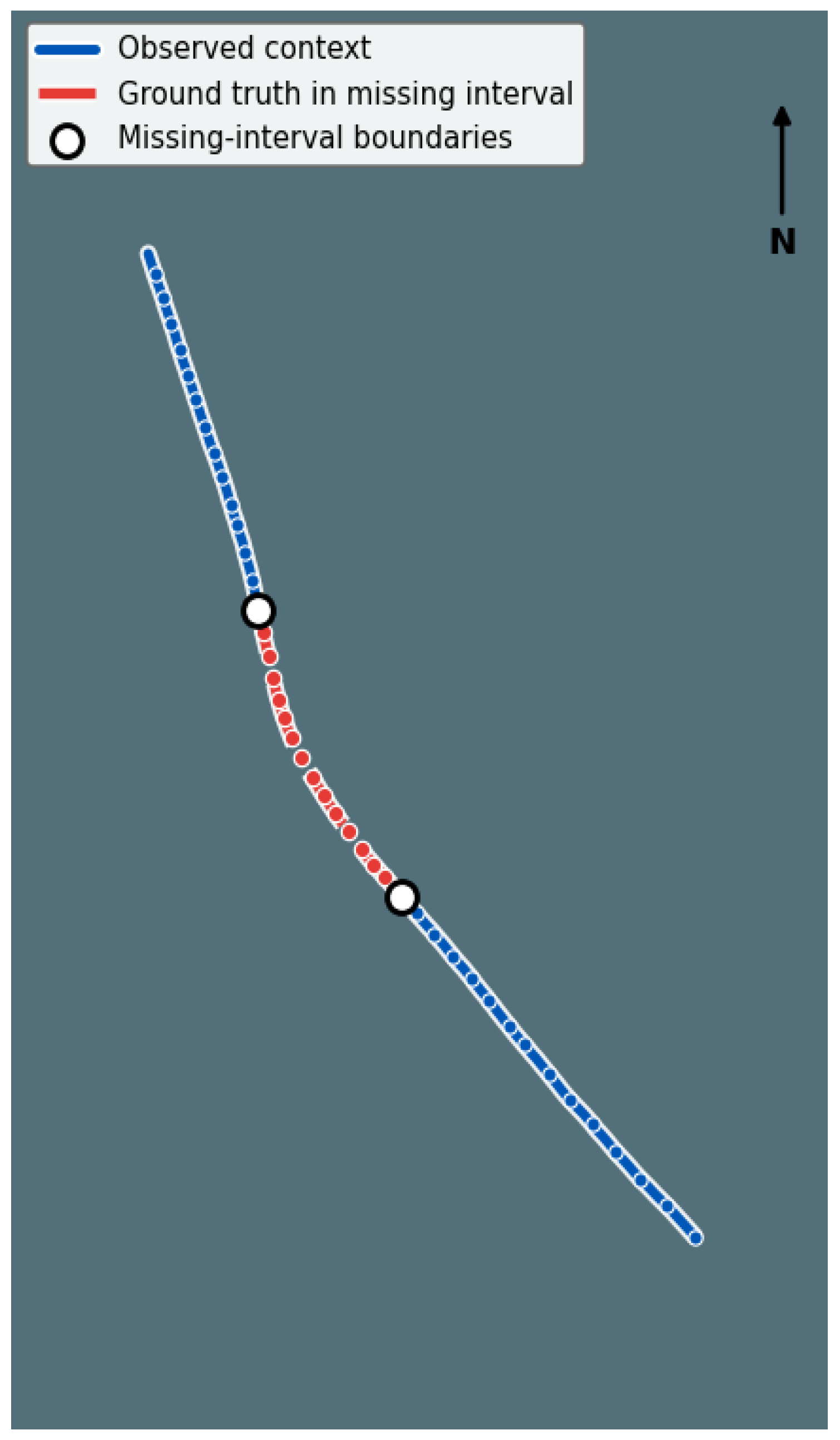
Figure 3 illustrates the AIS trajectory restoration problem formulated in this study and the overall processing framework of the proposed method. First, raw AIS data and vessel particulars are used as inputs, and model input sequences are constructed through spatial filtering, abnormal-data removal, trajectory segmentation, and fixed-length window generation. Subsequently, the central 30% of each 200-point sequence is masked to generate the missing segment to be restored, and Cubic Spline interpolation is applied to construct a preliminary trajectory. Based on this preliminary restoration, the proposed FiLM-conditioned Transformer predicts a bounded residual correction. The final restored trajectory is then obtained by combining the Cubic Spline-based preliminary restoration with the predicted residual correction.
Figure 3.
Overall framework of the proposed vessel-condition-aware AIS trajectory restoration method.
Accordingly, the AIS trajectory restoration problem considered in this study is not limited to geometrically connecting missing points. As illustrated in Figure 3, the proposed framework simultaneously exploits contextual information before and after the missing segment, the Cubic Spline-based preliminary restoration, and Transformer-based residual correction conditioned on vessel-specific information. Through this formulation, the model aims to preserve the overall trajectory shape while recovering local motion variations within the missing segment.
3.3. Preliminary Restoration Using Cubic Spline
In this study, Cubic Spline interpolation is employed as the preliminary restoration step to obtain a stable estimate of the overall trajectory shape within the missing segment. Cubic Spline interpolation constructs piecewise cubic polynomials based on the observed trajectory and generates a smooth curve by maintaining continuity of both the function values and their derivatives at the junctions between adjacent intervals. In the AIS trajectory restoration problem, Cubic Spline interpolation provides an initial estimate of the missing vessel positions using the observations available before and after the missing segment.
For the (i)-th trajectory sample, let () and () denote the sets of observed and missing time steps, respectively. Cubic Spline interpolation is independently applied to the latitude and longitude coordinates using the positions available in the observed region. Specifically, given the observed vessel position
separate spline functions are constructed for latitude and longitude and evaluated at the time steps belonging to the missing region. The preliminary restored position is then calculated as
where () and () denote the Cubic Spline functions constructed for the latitude and longitude coordinates of the (i)-th trajectory sample, respectively.
Using the interpolated positions, the preliminary trajectory over the entire sequence is defined
Accordingly, the original AIS positions are retained in the observed region, whereas the positions estimated by Cubic Spline interpolation are used in the missing region.
The preliminary trajectory constructed using Equation (8) provides a stable initial trajectory connecting the observations before and after the missing segment. Because Cubic Spline interpolation produces smoother curves than simple linear interpolation, it is useful for preserving the overall trend of vessel trajectories. However, Cubic Spline interpolation fundamentally relies on the temporal and geometric continuity between observed points. Consequently, when turning, deceleration, acceleration, or other complex maneuvering motions occur within the missing segment, it may not sufficiently capture the local motion variations in the actual vessel trajectory.
Therefore, the trajectory reconstructed by Cubic Spline interpolation is not used as the final restoration result in this study. Instead, it serves as a preliminary estimate to be further corrected by the subsequent Transformer-based restoration model. In other words, the proposed model is designed not to regenerate the missing trajectory directly from scratch, but to learn and correct the residual errors relative to the stable preliminary trajectory provided by Cubic Spline interpolation.
3.4. Vessel Condition Representation
Although the Cubic Spline-based preliminary restoration can provide a stable estimate of the overall trajectory shape using the observed positions before and after the missing segment, it does not explicitly account for vessel-specific differences in geometry and maneuvering-related conditions. Even when similar speed, course, and positional changes are observed, actual vessel trajectories may exhibit different motion patterns depending on vessel length, breadth, draft, gross tonnage, turning characteristics, and appendage-related characteristics. Therefore, in this study, vessel-specific condition information is constructed separately from the dynamic AIS information and subsequently used as conditional input to the FiLM-based Transformer restoration model.
The primary vessel particulars, AIS-derived motion variables, and derived variables used to construct the condition features are summarized in Table 1. Vessel length, breadth, draft, and gross tonnage are used to represent vessel-specific geometric differences, while displacement and motion-related variables describe local variations in the trajectory. Because detailed propeller and rudder specifications are generally unavailable in AIS datasets, appendage-related proxy descriptors are constructed using vessel-type-specific reference hulls. Cargo-family vessels are associated with the KRISO Container Ship (KCS), whereas conventional tanker vessels are associated with the KRISO Very Large Crude Carrier 2 (KVLCC2). This type-specific assignment avoids applying container-ship-based scaling relationships to tankers with substantially different hull forms and maneuvering characteristics.
Table 1.
Detailed variables used to construct vessel condition features.
Based on the variables listed in Table 1, vessel condition information is represented using dimensionless features. Directly using the absolute values of vessel particulars may introduce scale effects associated with differences in vessel size into the learning process. Therefore, the major variables are non-dimensionalized using vessel length and representative area scales. This allows trajectory variations associated with vessels of different sizes to be represented and compared within a common input space.
In this study, the vessel condition information is defined as a condition sequence constructed for each trajectory sample. For the (i)-th sample, the condition sequence is defined as
where () denotes the condition vector of the (i)-th trajectory sample at time step (t), and (Q) denotes the dimensionality of the condition features. A total of 22 condition features are used in this study. The condition vector consists of geometry-based information, motion- and maneuvering-related information, vessel-type-specific appendage proxy information, and vessel-family indicator information, as expressed in Equation (10):
Here, () denotes the geometry-based condition features constructed from vessel length, breadth, draft, gross tonnage, and displacement changes. The vector () represents the motion- and maneuvering-related condition features constructed from AIS trajectory variations and descriptors derived from the major coefficient concepts used in the MMG maneuvering model. The vector () represents the propeller- and rudder-related proxy features constructed using vessel-type-specific reference-hull relationships. Specifically, KCS-based scaling is applied to cargo-family vessels, whereas KVLCC2-based scaling is applied to tanker vessels. Finally, () represents two binary vessel-family indicators that explicitly distinguish cargo vessels from tankers. Some geometry- and motion-related variables vary over time and are therefore denoted by () and (). In contrast, the appendage-related proxy features and vessel-family indicators are fixed for each vessel and are denoted by () and (), respectively.
First, the geometry-based information is represented in a dimensionless form to account for differences in trajectory characteristics associated with vessel size. In this study, vessel length, breadth, draft, and gross tonnage are used to construct dimensionless geometric variables. In addition, the longitudinal and lateral displacement changes are normalized by vessel length to represent the relative displacement of vessels with different sizes. The geometry-based condition features are defined as
Next, the motion- and maneuvering-related condition features are constructed to represent local directional variations in the AIS trajectory and vessel-specific maneuvering response characteristics. Because AIS data do not directly provide actual control inputs or hydrodynamic coefficients, AIS-derived motion variables are combined with descriptors constructed with reference to the concepts of major coefficients used in MMG maneuvering models. Specifically, the condition features include the non-dimensional yaw rate representing directional changes, drift-angle-related variables representing the difference between the vessel heading and direction of motion, non-dimensional lateral velocity, and an estimated block coefficient reflecting vessel geometric characteristics.
To avoid discontinuities associated with angular variables, the drift angle is represented using its sine and cosine components rather than the raw angular value. This representation alleviates the discontinuity that may occur near and , allowing the model to learn directional differences as continuous inputs. Accordingly, the motion- and maneuvering-related condition features are defined as
Here, () denotes the non-dimensional yaw rate calculated from AIS-derived heading changes, and () denotes the drift angle calculated from the difference between the vessel heading and its direction of motion. () represents the non-dimensional lateral velocity, while () denotes the estimated block coefficient used to represent vessel geometric characteristics. () are descriptors constructed with reference to the concepts of sway-force and yaw-moment derivatives used in the MMG maneuvering model. In addition, () and () are used as correction descriptors associated with sway force and yaw moment. These variables are not intended to directly estimate the actual hydrodynamic derivatives of individual vessels. Accordingly, these variables should be interpreted as MMG-inspired conditioning descriptors rather than as measured vessel-specific maneuvering coefficients or validated hydrodynamic parameters. Instead, they are used as conditioning information to represent vessel-specific differences in maneuvering responses within the learning model.
Finally, the appendage-related condition features are constructed to represent relative differences in propeller- and rudder-related characteristics. Because the actual propeller diameter and rudder area of individual vessels are generally unavailable in AIS datasets, these quantities are not directly estimated. Instead, vessel-type-specific proxy values are constructed using the relative dimensional relationships of representative reference hulls. The KCS is assigned to cargo-family vessels, whereas the KVLCC2 is assigned to tanker vessels.
Let denote the reference hull assigned to the (i)-th vessel, defined as
The propeller- and rudder-related proxy values are obtained by scaling the reference-hull ratios according to the draft of the individual vessel. The resulting appendage-related condition features are defined as
Here, , , and denote the length, breadth, and draft of the (i)-th vessel, respectively. The terms , , and denote the propeller diameter, rudder area, and draft of the assigned reference hull. The reference values used for KCS are () m, () m, and () m2, while those used for KVLCC2 are () m, () m, and () m2.
These values are not intended to provide physical estimates of the actual propeller diameter or rudder area of individual vessels. Rather, they serve as dimensionless proxy descriptors that reflect vessel-family-specific reference relationships while reducing the direct influence of absolute vessel size.
The purpose of using KCS and KVLCC2 is not to approximate the actual propeller and rudder dimensions of individual vessels, but to provide vessel-family-specific normalized reference relationships when such detailed specifications are unavailable in AIS data. Accordingly, these variables are treated solely as auxiliary conditioning proxies rather than as vessel-specific maneuvering measurements or physical estimates of actual appendage dimensions.
Consequently, the final condition vector used in this study consists of 22 features and is expressed as
The condition vector in Equation (14) is arranged as a condition sequence with the same temporal length as the AIS input sequence. Vessel-specific static variables are repeated across all time steps within the same trajectory sample. In contrast, the time-varying condition features are derived after constructing the preliminary AIS sequence for the masked interval. Specifically, the longitudinal and lateral displacement changes are calculated from the Cubic-Spline-filled position sequence, while the yaw-rate- and drift-angle-related descriptors are calculated from the corresponding preliminary dynamic sequences. Therefore, the ground-truth AIS positions within the masked interval are not directly used to calculate these time-varying condition features. The resulting condition sequence, (), is subsequently provided to the condition branch for generating the FiLM parameters. For time steps belonging to the masked interval, the latitude, longitude, SOG, COG, and heading components correspond to the preliminary reconstructed values rather than the original AIS observations, and the associated change-related features are recalculated from this reconstructed sequence.
Unlike restoration approaches that rely solely on AIS coordinate sequences, the proposed vessel condition representation allows vessel size, geometry, maneuvering response, and appendage-related characteristics to be incorporated into the restoration process. In the subsequent stage, the condition branch receives () and generates the FiLM scaling parameter (γ) and shifting parameter (β). These parameters are applied to the Transformer hidden representations, enabling vessel-specific condition information to influence the residual correction process.
3.5. FiLM-Conditioned Transformer-Based AIS Trajectory Restoration
This section describes the FiLM-conditioned Transformer architecture for restoring missing AIS trajectories using the dynamic AIS inputs and vessel condition representation constructed in the preceding sections. The primary objective of the proposed model is not to completely replace the Cubic Spline-based preliminary restoration, but rather to use it as a stable reference trajectory while correcting local errors within the missing segment. Cubic Spline interpolation is effective in preserving the overall trajectory continuity by using observations before and after the missing segment; however, it has limited ability to represent detailed motion differences associated with vessel size, maneuvering response, and turning characteristics. Therefore, the proposed method performs Transformer-based residual correction on the preliminary trajectory generated by Cubic Spline interpolation while incorporating vessel-specific condition features through FiLM modulation.
The proposed model consists primarily of an AIS branch and a condition branch. The AIS branch receives the AIS sequence preliminarily restored by Cubic Spline interpolation and learns temporal motion patterns. The input sequence consists of dynamic AIS features including latitude, longitude, SOG, COG, heading, time intervals, change-related features, and a mask indicator. The mask indicator is used to distinguish whether each time step belongs to the observed or missing region. Through this representation, the Transformer can jointly consider the observations before and after the missing segment together with the preliminary restoration information to learn the temporal continuity of the trajectory.
In contrast, the condition branch receives the condition sequence defined in Equation (14) and represents vessel-specific geometric and maneuvering-related characteristics. Rather than directly reconstructing the AIS coordinate sequence, this branch generates FiLM parameters that modulate the Transformer hidden representations based on vessel condition information. Accordingly, even when similar AIS motion patterns are provided, the internal representation of the model can be adjusted according to vessel length, breadth, draft, gross tonnage, estimated block coefficient, maneuvering-related descriptors, and propeller- and rudder-related proxy features.
Let denote the Transformer hidden representation generated by the AIS branch, and let and denote the FiLM scaling and shifting parameters generated by the condition branch, respectively. The FiLM modulation is then applied as
where denotes the hidden representation modulated by vessel condition information, and ⊙ denotes element-wise multiplication. The term 1 + is used so that the original Transformer representation can be retained when the effect of the condition features is small. Thus, the FiLM layer directly modulates the hidden representation using vessel condition information while providing a stable modulation mechanism that avoids unnecessary changes to the original representation.
The FiLM-modulated hidden representation is subsequently used to predict position corrections within the missing segment. Rather than directly generating the final trajectory coordinates, the proposed model predicts a residual correction to be added to the Cubic Spline-based preliminary trajectory. This residual-learning strategy reduces the burden of reconstructing the entire trajectory from scratch and encourages the model to correct only the components that are insufficiently represented by Cubic Spline interpolation. In AIS trajectory restoration, preserving natural trajectory continuity with the observations immediately before and after the missing segment is particularly important. Therefore, performing local corrections with respect to a stable preliminary interpolation is suitable for the restoration problem considered in this study.
However, excessively large residual corrections may distort the stable trajectory shape provided by Cubic Spline interpolation. To prevent this, a gated bounded residual correction structure is introduced. The raw residual output is constrained using a hyperbolic tangent function, while a residual gate controls the correction intensity. The final residual correction is defined as
where denotes the final residual correction, denotes the raw residual output generated by the output layer, and denotes the sigmoid-activated residual gate, satisfying . The hyperbolic tangent constrains each component of the raw residual output to , and the coefficient determines the maximum component-wise correction range in the normalized coordinate space. In this study, is set to 0.06. Because the latitude and longitude coordinates are standardized using the training-data statistics, the corresponding correction range in the original geographic coordinate space is determined through inverse normalization.
The final restored trajectory is obtained by adding the predicted residual correction to the Cubic Spline-based preliminary trajectory:
Here, denotes the preliminary trajectory generated by Cubic Spline interpolation, denotes the predicted residual correction, and denotes the final trajectory restored by the proposed model. Through this architecture, the proposed method combines the stability of interpolation-based restoration with the temporal representation-learning capability of the Transformer. Furthermore, because vessel-specific condition features are incorporated into the residual correction process through FiLM modulation, the model can more effectively account for vessel-specific differences in trajectory restoration than methods that consider only geometric trajectory continuity.
3.6. Training Objective
The proposed model is trained primarily over the masked region corresponding to the missing trajectory segment. In this study, 60 consecutive AIS points corresponding to the central 30% of each input sequence are treated as the missing segment. The model is trained to minimize the error between the ground-truth AIS positions and the restored positions within this region. Although the observed region is provided as input to supply contextual information before and after the missing segment, the training loss is calculated only over the region requiring restoration.
Let denote the binary mask variable for time step (t) of the (i)-th sample. indicates that the corresponding time step belongs to the missing region, whereas indicates that it belongs to the observed region. Accordingly, the restoration loss is calculated only over the masked region as
where denotes the ground-truth AIS position coordinates and denotes the position coordinates restored by the proposed model. Equation (18) ensures that the model is optimized specifically to improve positional restoration accuracy within the missing segment rather than reconstructing the entire sequence equally.
In addition, a penalty term is introduced for the residual correction to prevent excessive modification of the Cubic Spline-based preliminary trajectory. Because the proposed model predicts a residual correction to be added to the Cubic Spline result rather than directly generating the final vessel position, excessively large corrections may degrade the stability of the preliminary interpolated trajectory. To mitigate this issue, the residual penalty is defined as
where denotes the bounded residual correction. The residual penalty suppresses unnecessary deviations from the Cubic Spline-based preliminary trajectory and encourages the model to perform only local corrections within the required range.
The final training loss is defined as the weighted sum of the restoration loss and the residual penalty:
where is a hyperparameter controlling the contribution of the residual penalty. The final objective function simultaneously minimizes the positional restoration error within the missing segment and constrains the model from excessively modifying the Cubic Spline-based preliminary restoration. Accordingly, the proposed model is trained to restore missing AIS trajectory segments by combining the stability of interpolation-based restoration with the expressive capability of Transformer-based residual correction.
4. Experiment and Result Analysis
4.1. Experimental Data and Implementation Settings
The experiments in this study were conducted using a dataset that combines AIS data collected in the waters near Ulsan Port with vessel particulars. The AIS data contain vessel identification, temporal information, positional information, and dynamic navigation information, while the vessel particulars are used to construct vessel-specific condition features. The major raw data variables used in this study and their corresponding roles in constructing the model inputs are summarized in Table 2.
Table 2.
Raw data variables used in this study.
Among the raw variables listed in Table 2, latitude and longitude are used as the target position coordinates for trajectory restoration. SOG, COG, heading, and the time intervals and change-related variables derived from timestamp information are used as AIS input features to represent the dynamic navigation state of the vessel. Vessel particulars are used to construct vessel-specific condition features. In particular, vessel length, breadth, draft, and gross tonnage are used to derive dimensionless geometric features and maneuvering-related descriptors.
Figure 4 shows representative AIS trajectories of tanker and cargo vessels used in the experiments. The yellow trajectories represent tanker vessels, whereas the blue trajectories represent cargo vessels. Both vessel types exhibit dense traffic patterns around the entrance and departure waters of Ulsan Port and along the major port approach routes. Trajectories extending toward offshore waters are also observed, indicating that the dataset used in this study contains diverse navigation patterns covering inner port waters, port approach routes, and offshore transit areas.
Figure 4.
Spatial distribution of tanker and cargo AIS trajectories in the Ulsan port area.
The entire dataset was divided into training, validation, and test sets at the trajectory level. This trajectory-wise split was applied to prevent windows generated from the same trajectory from being simultaneously included in different datasets and to evaluate restoration performance on held-out trajectories that were not used during training. Following the trajectory-wise split, 1331 trajectories were assigned to the training set, 285 trajectories to the validation set, and 286 trajectories to the test set.
Fixed-length windows of 200 AIS points were subsequently generated from each trajectory segment using a window stride of 50. Each input sequence therefore consists of 200 AIS points, and 60 consecutive points corresponding to the central 30% of the sequence were defined as the missing segment. This procedure resulted in 4369 training samples, 1010 validation samples, and 988 test samples.
The proposed model was implemented using PyTorch (version 2.5.1). The Transformer backbone consisted of two FiLM-conditioned Transformer blocks with a hidden dimension of 64, four self-attention heads, a feed-forward dimension of 128, and a dropout rate of 0.1. The AIS input sequence was projected into the 64-dimensional hidden space and combined with sinusoidal positional encoding. The condition branch mapped the vessel-condition sequence to the FiLM scaling and shifting parameters, and , which were applied after the self-attention and feed-forward operations in each Transformer block. The final hidden representations were passed through separate output and gate heads to generate the residual correction and sigmoid-activated residual gate, respectively. The model was trained using the Adam optimizer with a batch size of 16, a learning rate of , and a total of 80 epochs. Gradient clipping with a maximum norm of 1.0 was applied during training, and the model parameters corresponding to the lowest validation loss were retained for final evaluation on the test set.
To further evaluate vessel-independent restoration performance, an additional MMSI-wise data split was conducted using a subset of 403 MMSIs available for this evaluation. Unlike the trajectory-wise split used in the main experiment, all trajectory segments associated with the same MMSI were assigned exclusively to one of the training, validation, or test subsets. The split was performed at approximately 70%, 15%, and 15% of the available vessels while preserving the cargo–tanker composition. This resulted in 281 MMSIs (882 trajectories) for training, 60 MMSIs (159 trajectories) for validation, and 62 MMSIs (198 trajectories) for testing. No MMSI was shared across the three subsets. Following the same window-generation procedure, 2660 training samples, 431 validation samples, and 642 test samples were generated. All subsequent masking, preprocessing, model architecture, and training settings were kept consistent with those of the main experiment.
4.2. Evaluation Metrics and Performance Comparison
This section presents the comparison methods, evaluation metrics, and quantitative results used to assess the AIS trajectory restoration performance of the proposed model. Rather than directly predicting the missing positions, all learning-based comparison models are designed using a residual correction strategy. Specifically, Cubic Spline-based preliminary restoration is first performed, after which each learning-based model predicts an additional correction to the preliminary restoration. This experimental design enables a direct comparison between the interpolation performance of Cubic Spline itself and the residual correction performance of different sequence models.
Cubic Spline interpolation constructs continuous curves independently for the latitude and longitude coordinates using the observed positions before and after the missing segment, thereby generating a preliminary trajectory within the missing region. For the Cubic Spline-only method, the preliminary trajectory is directly used as the final restoration result without an additional learning process. In contrast, RNN, LSTM, BiLSTM, GRU, and the proposed model predict additional residual corrections with respect to the preliminary trajectory generated by Cubic Spline interpolation. Accordingly, the final restored position of the (k)-th learning-based comparison model is defined as
where denotes the preliminary restoration result generated by Cubic Spline interpolation, and denotes the residual correction predicted by the (k)-th learning-based model. Here, (k) represents one of the RNN, LSTM, BiLSTM, GRU, Seq2Seq, Transformer, and proposed residual-correction methods. The Cubic Spline-only baseline can be regarded as the case in which .
All comparison methods were evaluated using the same test data and missing-segment configuration. Linear interpolation and Cubic Spline were used as interpolation-based baselines. The learning-based comparison methods included RNN, LSTM, BiLSTM, GRU, Seq2Seq, and a Transformer without FiLM conditioning. Except for the interpolation-only baselines, the learning-based models refine the Cubic Spline preliminary trajectory through secondary or residual correction. The proposed method differs from these comparison models by incorporating vessel-condition information into the Transformer hidden representations through FiLM modulation and applying gated bounded residual correction.
The comparison methods used in this study are summarized in Table 3.
Table 3.
Comparison methods for AIS trajectory restoration.
The average Euclidean distance (AED) and maximum displacement error (MDE) were used to evaluate restoration performance within the missing segment.
Before calculating AED and MDE, the inverse-normalized latitude and longitude coordinates were transformed into a local Cartesian coordinate system expressed in meters using an equirectangular approximation. The origin was defined by the mean latitude and longitude of the evaluation trajectories. Specifically, the local coordinates were obtained as and , where m is the Earth radius, and denote latitude and longitude in radians, respectively, and and denote the reference latitude and longitude. AED and MDE were subsequently calculated using Euclidean distances in this local metric coordinate system.
All evaluation metrics were calculated only over the masked region corresponding to the actual restoration target rather than over the entire sequence. In this study, the set of time steps belonging to the missing region is denoted by , which corresponds to the time steps for which the binary mask variable is equal to 1.
where the corresponding variables denote the ground-truth AIS position coordinates of the (i)-th sample at time step (t) and the corresponding restored position coordinates. A lower AED indicates higher average positional restoration accuracy over the entire missing segment.
The MDE represents the largest distance error between the ground-truth and restored positions within the missing segment. Whereas AED measures the average restoration error over the missing region, MDE evaluates the maximum deviation of the restored trajectory from the ground-truth trajectory. The MDE for the (i)-th test sample is defined as
A lower MDE indicates that the restored trajectory is less likely to deviate substantially from the ground-truth trajectory at any point within the missing segment. Therefore, the combined use of AED and MDE allows both the average restoration accuracy and the maximum positional deviation within the missing region to be evaluated.
The overall performance of each model was calculated by averaging the AED and MDE values over all test samples. Let denote the total number of test samples. The mean AED and MDE are calculated as
In addition, an improvement rate was calculated to quantitatively evaluate the extent to which each learning-based correction model improves upon the Cubic Spline baseline. For an evaluation metric (E), corresponding to either AED or MDE, the improvement rate is defined as
where denotes the performance of the Cubic Spline baseline and denotes the performance of the comparison model. A larger improvement rate indicates a greater performance improvement achieved through residual correction relative to the Cubic Spline preliminary restoration.
Table 4 compares the AIS trajectory restoration performance of the interpolation-based baselines, recurrent residual correction models, Seq2Seq-based secondary restoration model, Plain Transformer, and the proposed FiLM-conditioned Transformer in terms of AED and MDE. Cubic Spline interpolation achieved an AED of 145.4336 m and an MDE of 286.0341 m, while Linear interpolation achieved an AED of 139.9979 m and an MDE of 255.3363 m. The learning-based models showed different levels of improvement depending on their architectures and evaluation metrics.
Table 4.
Comparison of AIS trajectory restoration performance.
The additionally evaluated Seq2Seq-based secondary restoration model achieved an AED of 146.0848 m and an MDE of 286.1582 m, whereas the Plain Transformer without FiLM conditioning achieved an AED of 134.3563 m and an MDE of 268.5889 m. The proposed FiLM-conditioned Transformer achieved an AED of 134.1975 m and an MDE of 269.4482 m. Relative to the Cubic Spline baseline, the proposed method improved AED by 7.7259% and MDE by 5.7986%. Compared with the Seq2Seq model, the proposed method reduced both AED and MDE, while compared with the Plain Transformer, it achieved a slightly lower AED but a slightly higher MDE.
These results indicate that the proposed method provides the lowest AED among the evaluated methods, demonstrating an advantage in terms of average positional restoration accuracy. However, the MDE results show a different tendency. Linear interpolation achieved the lowest MDE among the comparison methods, and the Plain Transformer also achieved a slightly lower MDE than the proposed model. Therefore, the proposed method should not be interpreted as uniformly outperforming all comparison methods for every error measure. Rather, its main advantage in the present experiment is the reduction in the average positional error while maintaining a comparable level of maximum displacement error.
The comparison between the Plain Transformer and the proposed FiLM-conditioned Transformer further shows that the difference between the two Transformer-based models is relatively small in the overall AED and MDE metrics. The proposed model achieved a modest improvement in AED, whereas the Plain Transformer showed a slightly lower MDE. This result suggests that the contribution of vessel-condition-aware FiLM modulation cannot be fully characterized by the aggregate performance comparison alone.
To further examine the robustness of the learning-based models to random initialization, additional repeated-training experiments were conducted using five independent random seeds for the BiLSTM, Plain Transformer, and proposed model. The mean, standard deviation, and 95% confidence intervals of AED and MDE across the five runs are summarized in Table 5. The proposed method achieved an AED of 134.6769 ± 1.2577 m and an MDE of 268.9301 ± 1.4206 m. The corresponding values were 135.8526 ± 2.2213 m and 267.1873 ± 1.0709 m for BiLSTM, and 133.9660 ± 0.8599 m and 268.4689 ± 0.4745 m for the Plain Transformer. These results show that the performance differences among the learning-based models are relatively modest and depend on the evaluation metric.
Table 5.
Repeated-run robustness analysis over five independent random seeds.
Because multiple overlapping windows can be generated from the same parent trajectory, statistical comparisons were additionally performed after aggregating the window-level errors within each parent trajectory. For the comparison between the proposed method and BiLSTM, the trajectory-level paired difference in AED (Proposed—BiLSTM) was −3.0328 m, with a 95% bootstrap confidence interval of −5.4236 to −0.7016 m and a Wilcoxon signed-rank test p-value of 0.0064. For MDE, the corresponding difference was −0.5593 m (95% bootstrap CI: −4.2696 to 3.1447 m; p = 0.7410). Compared with the Plain Transformer, the paired AED difference was −0.2278 m (95% bootstrap CI: −1.4892 to 0.9647 m; p = 0.6513), while the MDE difference was −0.7734 m (95% bootstrap CI: −2.7695 to 1.1829 m; p = 0.9301). These results indicate that the proposed method achieved a statistically significant reduction in trajectory-level AED relative to BiLSTM, whereas the corresponding MDE difference was not statistically significant. In addition, neither AED nor MDE differed significantly between the proposed method and the Plain Transformer. Accordingly, the individual contributions of the conditioning information and FiLM modulation are further examined through the ablation analyses presented in the following sections.
As shown in Table 6, a condition-shuffling analysis was first conducted to examine whether restoration performance depends on the correct correspondence between the AIS trajectory and its vessel-specific condition information. When the condition features were randomly shuffled across test samples, while the AIS sequence and Cubic Spline preliminary trajectory were kept unchanged, the AED increased from 134.1975 m to 136.9591 m and the MDE increased from 269.4482 m to 273.0670 m. This result indicates that disrupting the correspondence between trajectory and condition information degrades restoration performance.
Table 6.
Effect of vessel condition features on restoration performance.
A Plain Transformer without FiLM conditioning was additionally evaluated to distinguish the effect of vessel-condition information from that of the Transformer architecture itself. The Plain Transformer achieved an AED of 134.3563 m and an MDE of 268.5889 m. Compared with this configuration, the proposed FiLM-conditioned model achieved a slightly lower AED of 134.1975 m, while the Plain Transformer showed a slightly lower MDE. Thus, the effect of FiLM conditioning was relatively modest when assessed using the overall AED and MDE metrics.
An alternative conditioning strategy based on direct feature concatenation was also evaluated. In this configuration, the AIS and vessel-condition features were directly concatenated before being processed by the Transformer, resulting in an AED of 137.5746 m and an MDE of 274.6849 m. Both errors were higher than those of the proposed model. This result indicates that simply providing the condition variables does not necessarily improve restoration performance and that the manner in which the condition information is incorporated into the model is important.
Overall, the condition-shuffling, no-condition, and direct-concatenation experiments show that restoration performance is affected by both the correspondence of the vessel-condition information and the conditioning mechanism. In the present experiment, FiLM-based conditioning achieved lower average positional error than both the Plain Transformer and the direct-concatenation model, although the Plain Transformer produced a slightly lower MDE.
4.3. Vessel-Independent Evaluation Using MMSI-Wise Splitting
To further assess the vessel-independent generalization capability of the proposed method, an additional evaluation was conducted using the MMSI-wise data split described in Section 4.1. In contrast to the trajectory-wise split used in the main experiment, all trajectory segments associated with a given MMSI were assigned exclusively to one of the training, validation, or test subsets. Consequently, the vessels included in the test set were completely unseen during model training and validation. The MMSI-wise test set consisted of 62 previously unseen vessels, comprising 198 trajectory segments and 642 test windows.
For this additional evaluation, Cubic Spline interpolation, BiLSTM-based residual correction, and the proposed FiLM-conditioned Transformer were compared. BiLSTM was selected as the representative recurrent baseline because it achieved the best performance among the recurrent models in the main trajectory-wise experiment. For the proposed model, hyperparameter selection was performed exclusively on the validation set, without using the test set. The final configuration was selected according to the lowest validation restoration loss, and the test set was evaluated only after the model configuration had been fixed.
As shown in Table 7, Cubic Spline interpolation achieved an AED of 151.0069 m and an MDE of 298.1242 m under the MMSI-wise split. The proposed FiLM-conditioned Transformer reduced the AED to 128.8441 m and the MDE to 267.4611 m, corresponding to improvements of 14.68% and 10.29%, respectively, relative to Cubic Spline interpolation. These results demonstrate that the proposed residual-correction framework maintained its ability to improve the preliminary interpolated trajectory even when applied to vessels that were not observed during training.
Table 7.
Vessel-independent trajectory restoration performance under MMSI-wise splitting.
Compared with the BiLSTM baseline, the proposed method achieved a lower AED of 128.8441 m compared with 130.5519 m, corresponding to an additional reduction of approximately 1.71 m. This indicates that the proposed method provided improved average positional restoration accuracy under the vessel-independent evaluation. In contrast, BiLSTM achieved a slightly lower MDE of 266.4615 m compared with 267.4611 m for the proposed method, a difference of approximately 1.00 m. Thus, the proposed method achieved the best average restoration accuracy, whereas the two learning-based methods exhibited very similar performance in terms of maximum positional deviation.
Overall, the MMSI-wise results indicate that the performance improvement of the proposed method was maintained even after eliminating vessel identity overlap between the training and test sets. In particular, the reduction in AED suggests that the FiLM-conditioned Transformer can transfer the learned trajectory-correction patterns to previously unseen vessels. However, the marginal difference in MDE relative to BiLSTM also indicates that vessel-independent generalization remains challenging, particularly for trajectories containing relatively large local deviations.
4.4. Sensitivity of the Proposed Model to Different Missing Patterns
To further investigate the sensitivity of the proposed model to different missing-segment configurations, additional evaluations were conducted by varying the missing ratio, location, and structure of the masked interval. The proposed model trained under the original central 30% masking condition was used without retraining. Five test conditions were considered: central 20%, central 30%, central 40%, randomly positioned contiguous 30%, and multiple irregular gaps with a total missing ratio of 30%. The central 30% condition corresponds to the main experimental setting, whereas the remaining conditions were used to examine how the trained model responds to missing patterns that differ from those encountered during training.
As shown in Table 8, the restoration performance of the proposed model varied according to the missing-segment configuration. Under the original central 30% condition, the model achieved an AED of 134.1975 m and an MDE of 269.4482 m. When the missing ratio was changed to 20% and 40%, the corresponding AED values were 156.0049 m and 160.9806 m, respectively. This indicates that the length of the missing interval influences restoration performance even when the missing segment remains centered within the sequence.
Table 8.
Sensitivity of the proposed model to different missing-segment configurations.
A further variation in restoration error was observed when the location or structural form of the missing segment was changed. Under the randomly positioned contiguous 30% condition, the model yielded an AED of 177.9109 m and an MDE of 311.0258 m. For the multiple irregular-gap condition, the corresponding values were 91.1091 m and 201.9613 m. Because the spatial and temporal characteristics of the masked regions differ across these conditions, the absolute error values should not be interpreted solely as a direct ranking of task difficulty.
Overall, the results indicate that the proposed model is sensitive to the missing-pattern distribution. Since the model was trained using a fixed central 30% missing segment, its learned residual-correction behavior may be partially specialized to this training configuration. These findings suggest that incorporating variable missing ratios, randomized missing locations, and multiple-gap masking during training could improve robustness to more diverse AIS data-loss patterns.
4.5. Performance According to Missing-Segment Characteristics
Although the same number of AIS points was masked in the main experiment, the actual temporal and navigational characteristics of the missing interval differed among trajectory samples. Therefore, an additional post hoc analysis was conducted to examine the restoration performance of the proposed model according to gap duration, traveled distance, and maneuvering intensity. For each characteristic, the test samples were divided into three groups using the 33.3rd and 66.7th percentiles. Gap duration and traveled distance were categorized into short, medium, and long groups, whereas maneuvering intensity was categorized into low, medium, and high groups. Maneuvering intensity was calculated as the cumulative absolute heading change normalized by the elapsed time of the missing interval. Ground-truth information within the masked interval was used only for this post hoc categorization and was not provided to the model during training or inference.
As shown in Table 9, restoration performance varied substantially across the different missing-segment characteristics. For gap duration, the medium-duration group exhibited the largest errors, with an AED of 175.1022 m and an MDE of 342.8081 m, whereas the short- and long-duration groups showed lower AED values of 113.4358 m and 111.8914 m, respectively. Thus, the restoration error did not increase monotonically with the elapsed duration of the missing interval.
Table 9.
Restoration performance of the proposed model according to missing-segment characteristics.
A similar non-monotonic relationship was observed for traveled distance. The medium-distance group showed the highest AED and MDE values of 183.7999 m and 357.2012 m, respectively. In comparison, the short-distance group achieved an AED of 94.2370 m, while the long-distance group achieved an AED of 124.5555 m. These results indicate that the physical distance traveled during the missing interval alone does not fully determine the difficulty of trajectory restoration.
Restoration performance also differed according to maneuvering intensity. The low-intensity group achieved the lowest AED and MDE values of 81.2665 m and 164.9685 m, respectively, whereas the medium-intensity group exhibited the largest errors, with an AED of 194.7701 m and an MDE of 383.2470 m. The high-intensity group showed intermediate errors of 127.1068 m and 261.1887 m. Therefore, although relatively stable motion was associated with lower restoration errors, the relationship between maneuvering intensity and restoration difficulty was not strictly monotonic.
Overall, these results indicate that restoration difficulty cannot be explained solely by the number of missing AIS points or by a single characteristic such as gap duration, traveled distance, or maneuvering intensity. Instead, restoration performance appears to depend on the combined temporal and navigational characteristics of individual trajectory segments. This stratified analysis therefore complements the overall AED and MDE results by showing that the restoration accuracy of the proposed model varies across different missing-segment conditions.
4.6. Qualitative Analysis of Trajectory Restoration Results
Figure 5 presents representative examples of AIS trajectory restoration results selected from the test dataset. In the figure, the blue points denote the observed AIS points before and after the missing segment, while the red trajectory represents the ground-truth trajectory within the central missing segment. The green dashed line indicates the preliminary restoration result generated by Cubic Spline interpolation, and the yellow trajectory denotes the final restoration result of the proposed FiLM-conditioned Transformer-based model.
Figure 5.
Representative AIS trajectory restoration results of the proposed method.
Because Cubic Spline interpolation smoothly connects the observed positions before and after the missing segment, it generally provides a stable preliminary restoration result. As shown in Figure 5, the Cubic Spline result does not deviate substantially from the overall trajectory trend. However, some local positional discrepancies from the ground-truth trajectory can still be observed within the missing segment. This can be interpreted as a limitation of simple interpolation methods, which primarily rely on geometric continuity between observed points.
In contrast, the proposed model does not completely replace the Cubic Spline preliminary trajectory, but instead performs bounded residual correction with respect to it. In Figure 5, the restoration result of the proposed model preserves the overall path shape of the Cubic Spline result while showing a tendency to be corrected toward the ground-truth trajectory in some parts of the missing segment. This suggests that the proposed model performs local position refinement using the contextual information surrounding the missing segment together with vessel condition features, while retaining the stability of the interpolation-based preliminary restoration.
To complement the qualitative examples in Figure 5, Table 10 presents the restoration performance separately for cargo and tanker vessels. This family-wise evaluation was conducted to examine whether the proposed method provides consistent restoration performance across vessel categories with different geometric and maneuvering characteristics.
Table 10.
Family-wise trajectory restoration performance on the test dataset.
As shown in Table 10, the restoration performance differed between cargo and tanker vessels. For cargo vessels, the proposed method achieved the lowest AED and MDE among all comparison methods, with values of 85.8893 m and 169.6534 m, respectively. Compared with Cubic Spline interpolation, the proposed method reduced the AED by approximately 15.87% and the MDE by approximately 13.06%. It also outperformed the Cubic Spline + Transformer model, which achieved an AED of 87.4062 m and an MDE of 177.9821 m. These results indicate that the proposed vessel-condition-aware correction framework was particularly effective for the cargo-vessel trajectories considered in the test dataset.
For tanker vessels, the proposed method achieved the lowest AED of 146.8156 m, corresponding to an approximately 6.34% reduction relative to the Cubic Spline baseline. The MDE of the proposed method was 295.5147 m, representing an approximately 4.60% reduction from the Cubic Spline baseline. The Cubic Spline + Transformer model achieved a slightly lower tanker MDE of 294.8674 m, although its AED was slightly higher at 147.1420 m. Therefore, the two Transformer-based models showed highly comparable performance for tanker trajectories, with the proposed method providing a small advantage in average positional accuracy.
The Seq2Seq-based model showed comparatively larger errors, with AED/MDE values of 101.8730/194.3945 m for cargo vessels and 157.6327/310.1267 m for tanker vessels. Linear interpolation achieved an AED/MDE of 96.2898/173.7592 m for cargo vessels and 151.4150/296.6451 m for tanker vessels. Although these conventional and sequence-based methods provided competitive results for some metrics, the proposed method consistently achieved lower AED values for both vessel families.
Overall, the family-wise results show that the proposed method improved the average trajectory restoration accuracy for both cargo and tanker vessels relative to the interpolation and recurrent comparison methods. The improvement was more pronounced for cargo vessels, for which the proposed method achieved the lowest values for both AED and MDE. For tanker vessels, the proposed method achieved the lowest AED, whereas the Plain Transformer exhibited a marginally lower MDE. This indicates that the effect of vessel-condition-aware FiLM modulation may vary depending on vessel family and evaluation metric, which is further investigated through the subsequent ablation analysis.
4.7. Ablation Analysis of Model Components
Ablation experiments were conducted to investigate the contribution of the major components of the proposed framework. The Plain Transformer and direct-concatenation configurations were evaluated as alternative conditioning strategies, as described above, while the component-removal experiments included removal of the geometry features, maneuvering-related features, appendage-related proxy features, and the bounded residual correction mechanism. The component-removal results are summarized in Table 10.
As shown in Table 11, removing the vessel-geometry features increased the AED from 134.1975 m to 134.9388 m and the MDE from 269.4482 m to 269.8108 m. A larger degradation was observed when the maneuvering-related features were removed, resulting in an AED of 136.6095 m and an MDE of 270.4138 m. These results indicate that both geometry- and maneuvering-related condition information contribute to restoration performance, with the maneuvering-related descriptors showing a more pronounced contribution under the present experimental setting.
Table 11.
Ablation analysis of the proposed AIS trajectory restoration framework on the test dataset.
The model without the appendage-related proxy features achieved an AED of 134.3100 m and an MDE of 269.3979 m. Compared with the full proposed model, the AED increased slightly, whereas the MDE decreased by only 0.0503 m. Therefore, the incremental contribution of the appendage-related proxy descriptors was relatively limited compared with that of the geometry and maneuvering-related features. This result suggests that these proxy variables may provide supplementary vessel-condition information, while their individual effect on the aggregate restoration metrics remains modest in the present dataset.
The largest performance degradation was observed when the bounded residual correction mechanism was removed. In this configuration, the AED increased to 137.9372 m and the MDE increased to 277.9427 m, corresponding to increases of 3.7397 m and 8.4945 m, respectively, relative to the full proposed model. This result supports the role of the bounded residual mechanism in preventing excessive correction of the Cubic Spline preliminary trajectory and maintaining stable trajectory restoration.
Overall, the component-level ablation results indicate that the maneuvering-related condition features and bounded residual correction mechanism make clear contributions to restoration performance. Geometry features also provided a smaller positive contribution, whereas the additional effect of the appendage-related proxy descriptors was comparatively limited. Together with the conditioning-strategy analyses presented above, these results provide a more detailed assessment of the individual components constituting the proposed framework.
4.8. Discussion on Restoration Performance and Condition-Aware Residual Correction
Taken together, the quantitative and qualitative results indicate that the proposed FiLM-conditioned Transformer-based restoration method is effective in correcting detailed positional errors within the missing segment while preserving the stability of the Cubic Spline-based preliminary restoration. Cubic Spline interpolation has the advantage of smoothly connecting the observations before and after the missing segment, but it has limited capability to directly reflect local motion variations or subtle curvature changes that may occur within the missing interval. In contrast, the proposed model does not use the Cubic Spline result as the final output without modification. Instead, it performs residual correction within a bounded range with respect to the preliminary trajectory, thereby combining the stability of interpolation-based restoration with the expressive capability of learning-based correction.
The comparison with recurrent residual correction models further suggests that Transformer-based contextual representation may be more suitable than simple recurrent temporal structures for capturing the information surrounding the missing segment. Bidirectional recurrent models such as BiLSTM have the advantage of utilizing contextual information from both before and after the missing interval. However, the proposed model can capture relationships among multiple time steps more flexibly through the self-attention mechanism. This structural difference may have contributed to the lower AED and MDE achieved by the proposed method in the restoration of the central missing segment.
The contribution of vessel condition features was also confirmed through the condition-shuffling analysis. The fact that restoration performance deteriorated when only the condition features were randomly shuffled, while the AIS input sequence and Cubic Spline preliminary trajectory were kept unchanged, indicates that the proposed model makes meaningful use of vessel particulars and maneuvering-related information during the restoration process rather than treating them as merely auxiliary inputs. This result suggests that vessel size, geometry, and motion characteristics can influence missing trajectory restoration, and that incorporating such information into the Transformer representation through FiLM modulation is an effective strategy.
Nevertheless, several limitations remain. First, in this study, a continuous missing segment corresponding to the central 30% of each input sequence was artificially generated for training and evaluation. Although this setting is appropriate for comparing model performance under controlled and identical conditions, the missing patterns observed in real AIS data may vary more widely in terms of missing length, missing location, and occurrence pattern. Therefore, further validation under diverse missing ratios and irregular missing patterns is needed in future work. In addition, because this study focused on tanker and cargo vessels operating in the waters near Ulsan Port, the present results should be interpreted within this experimental scope, and external validation using AIS data from other sea areas and a broader range of vessel types is required to further assess generalization capability.
5. Conclusions
This study proposed a FiLM-conditioned Transformer framework for restoring continuous missing segments in AIS trajectories. AIS data collected in the waters near Ulsan Port were divided into sequences of 200 points, and the central 60 points, corresponding to 30% of each sequence, were treated as missing. The proposed method first generated a preliminary trajectory using Cubic Spline interpolation and then applied gated bounded residual correction to refine the missing segment. A 22-dimensional vessel condition sequence was incorporated through FiLM modulation to account for differences in vessel geometry, motion, and maneuvering characteristics. In particular, KCS-based reference-hull proxy features were assigned to cargo-family vessels, whereas KVLCC2-based proxy features were assigned to tanker vessels.
The experimental results showed that the proposed method achieved an AED of 134.20 m and an MDE of 269.45 m, corresponding to improvements of 7.73% and 5.80%, respectively, over the Cubic Spline baseline. The proposed method also achieved lower AED and MDE values than the RNN-, LSTM-, BiLSTM-, and GRU-based residual correction models. These results indicate that combining the stable geometric continuity provided by Cubic Spline interpolation with the contextual representation capability of a Transformer can improve both average restoration accuracy and maximum positional deviation within the missing segment.
The condition-shuffling analysis further showed that disrupting the correspondence between the AIS trajectory and its vessel condition sequence increased both AED and MDE. This result supports the contribution of vessel-specific condition information to the restoration process and indicates that the FiLM layers make meaningful use of vessel particulars, maneuvering-related descriptors, vessel-family indicators, and type-specific reference-hull proxy features. Therefore, the proposed method provides a vessel-aware restoration framework that extends conventional interpolation-based approaches beyond geometric trajectory continuity alone.
Future work should evaluate the proposed method under varying missing ratios, irregularly located gaps, multiple missing intervals, and non-uniform AIS sampling intervals. Its generalization capability should also be examined using trajectories collected from different sea areas and a broader range of vessel types. In particular, systematic ablation experiments are required to separately quantify the effects of vessel-family classification and propulsion- and steering-related proxy features. Comparisons among a model without vessel conditions, a model using a common reference hull for all vessels, and the proposed vessel-type-specific KCS/KVLCC2 configuration would clarify the contribution of the reference-hull assignment. Additional experiments excluding the vessel-family indicators or the propeller- and rudder-related proxy features should also be conducted to identify their individual effects. Finally, incorporating actual vessel-specific parameters, such as propeller diameter, rudder area, engine power, and shaft rotational speed, would enable direct comparison between reference-hull-based proxy descriptors and measured propulsion and maneuvering information.
Author Contributions
Conceptualization, S.K. (Seokho Kang) and H.L.; Methodology, S.K. (Seokho Kang) and H.L.; Validation, S.K. (Seokho Kang); Formal analysis, S.K. (Seokho Kang); Investigation, S.K. (Seokho Kang); Resources, S.K. (Sewon Kim); Data curation, S.K. (Seokho Kang); Writing—original draft, S.K. (Seokho Kang); Writing—review and editing, S.K. (Seokho Kang) and S.K. (Sewon Kim); Visualization, S.K. (Seokho Kang); Supervision, S.K. (Sewon Kim); Project administration, S.K. (Sewon Kim); Funding acquisition, S.K. (Sewon Kim) All authors have read and agreed to the published version of the manuscript.
Funding
This research has received partial support from the Korea Institute of Marine Science & Technology Promotion (KIMST), funded by the Ministry of Oceans and Fisheries (RS-2023-00256127) (65%). This work was also supported by the Ministry of Trade, Industry and Energy (MOTIE) and Korea Institute for Advancement of Technology (KIAT) through the International Cooperative R&D Program (P0028244) (15%). Further support was provided by the Ministry of Science and ICT (MSIT), Republic of Korea, through the ICT Challenge and Advanced Network of HRD (ICAN) program (IITP-2026-RS-2022-00156345), under the supervision of the Institute for Information and Communications Technology, Planning and Evaluation (IITP) (20%).
Data Availability Statement
Data available on request due to restrictions. The data presented in this study are available on request from the corresponding author.
Conflicts of Interest
The authors declare no conflicts of interest.
References
- Pallotta, G.; Vespe, M.; Bryan, K. Vessel pattern knowledge discovery from AIS data: A framework for anomaly detection and route prediction. Entropy 2013, 15, 2218–2245. [Google Scholar] [CrossRef] [Scilit]
- Tu, E.; Zhang, G.; Rachmawati, L.; Rajabally, E.; Huang, G.-B. Exploiting AIS data for intelligent maritime navigation: A comprehensive survey from data to methodology. IEEE Trans. Intell. Transp. Syst. 2018, 19, 1559–1582. [Google Scholar] [CrossRef] [Scilit]
- Yang, D.; Wu, L.; Wang, S.; Jia, H.; Li, K.X. How big data enriches maritime research—A critical review of Automatic Identification System (AIS) data applications. Transp. Rev. 2019, 39, 755–773. [Google Scholar] [CrossRef] [Scilit]
- Harati-Mokhtari, A.; Brooks, P.; Wall, A.; Wang, J. Automatic Identification System (AIS): Data reliability and human error implications. J. Navig. 2007, 60, 373–389. [Google Scholar] [CrossRef] [Scilit]
- Last, P.; Hering-Bertram, M.; Linsen, L. How automatic identification system (AIS) antenna setup affects AIS signal quality. Ocean Eng. 2015, 100, 83–89. [Google Scholar] [CrossRef] [Scilit]
- Nguyen, V.-S.; Im, N.; Lee, S. The interpolation method for the missing AIS data of ship. J. Navig. Port Res. 2015, 39, 377–384. [Google Scholar] [CrossRef] [Scilit]
- Zhang, L.; Meng, Q.; Xiao, Z.; Fu, X. A novel ship trajectory reconstruction approach using AIS data. Ocean Eng. 2018, 159, 165–174. [Google Scholar] [CrossRef] [Scilit]
- Guo, S.; Mou, J.; Chen, L.; Chen, P. Improved kinematic interpolation for AIS trajectory reconstruction. Ocean Eng. 2021, 234, 109256. [Google Scholar] [CrossRef] [Scilit]
- Yan, R.; Mo, H.; Yang, D.; Wang, S. Development of denoising and compression algorithms for AIS-based vessel trajectories. Ocean Eng. 2022, 252, 111207. [Google Scholar] [CrossRef] [Scilit]
- Zaman, B.; Marijan, D.; Kholodna, T. Interpolation-based inference of vessel trajectory waypoints from sparse AIS data in maritime. J. Mar. Sci. Eng. 2023, 11, 615. [Google Scholar] [CrossRef] [Scilit]
- Ye, L.; Chen, X.; Liu, H.; Zhang, R.; Li, J.; Lu, C.; Zhao, Y. A study of multi-step sparse vessel trajectory restoration based on feature correlation. Appl. Sci. 2024, 14, 4057. [Google Scholar] [CrossRef] [Scilit]
- Liang, M.; Su, J.; Liu, R.W.; Lam, J.S.L. AISClean: AIS data-driven vessel trajectory reconstruction under uncertain conditions. Ocean Eng. 2024, 306, 117987. [Google Scholar] [CrossRef] [Scilit]
- Wu, H.; Hu, L.; Li, X.; Wang, C.; Ye, Z. A novel ship trajectory reconstruction approach based on low-rank tensor completion. Ocean Eng. 2024, 310, 118724. [Google Scholar] [CrossRef] [Scilit]
- Wang, W.; Xiong, W.; Chen, L.; Chen, H. TrajDiff: A method for vessel trajectory imputation utilizing resampled conditional diffusion models. Results Eng. 2025, 28, 107279. [Google Scholar] [CrossRef] [Scilit]
- Spiliopoulos, G.; Troupiotis-Kapeliaris, A.; Patroumpas, K.; Liapis, N.; Skoutas, D.; Zissis, D.; Bikakis, N. Data-driven trajectory imputation for vessel mobility analysis. In Proceedings of the 29th International Conference on Extending Database Technology (EDBT 2026), Tampere, Finland, 24–27 March 2026; pp. 659–667. [Google Scholar] [CrossRef]
- Capobianco, S.; Millefiori, L.M.; Forti, N.; Braca, P.; Willett, P. Deep learning methods for vessel trajectory prediction based on recurrent neural networks. IEEE Trans. Aerosp. Electron. Syst. 2021, 57, 4329–4346. [Google Scholar] [CrossRef] [Scilit]
- Li, H.; Jiao, H.; Yang, Z. AIS data-driven ship trajectory prediction modelling and analysis based on machine learning and deep learning methods. Transp. Res. Part E Logist. Transp. Rev. 2023, 175, 103152. [Google Scholar] [CrossRef] [Scilit]
- Zhang, Y.; Han, Z.; Zhou, X.; Li, B.; Zhang, L.; Zhen, E.; Wang, S.; Zhao, Z.; Guo, Z. METO-S2S: A S2S based vessel trajectory prediction method with Multiple-semantic Encoder and Type-Oriented Decoder. Ocean Eng. 2023, 277, 114248. [Google Scholar] [CrossRef] [Scilit]
- Jiang, D.; Shi, G.; Li, N.; Ma, L.; Li, W.; Shi, J. TRFM-LS: Transformer-based deep learning method for vessel trajectory prediction. J. Mar. Sci. Eng. 2023, 11, 880. [Google Scholar] [CrossRef] [Scilit]
- Nguyen, D.; Fablet, R. A Transformer network with sparse augmented data representation and cross entropy loss for AIS-based vessel trajectory prediction. IEEE Access 2024, 12, 21596–21609. [Google Scholar] [CrossRef] [Scilit]
- Yasukawa, H.; Yoshimura, Y. Introduction of MMG standard method for ship maneuvering predictions. J. Mar. Sci. Technol. 2015, 20, 37–52. [Google Scholar] [CrossRef] [Scilit]
- Yang, X.; Han, Z.; Zhang, Y.; Liu, H.; Liu, S.; Ai, W.; Liu, J. VEPO-S2S: A vessel portrait oriented trajectory prediction model based on S2S framework. Appl. Sci. 2024, 14, 6344. [Google Scholar] [CrossRef] [Scilit]
- Perez, E.; Strub, F.; de Vries, H.; Dumoulin, V.; Courville, A. FiLM: Visual reasoning with a general conditioning layer. Proc. AAAI Conf. Artif. Intell. 2018, 32, 3942–3951. [Google Scholar] [CrossRef] [Scilit]
- Xue, H. Fractional-order gradient descent with momentum for RBF neural network-based AIS trajectory restoration. Soft Comput. 2021, 25, 869–882. [Google Scholar] [CrossRef] [Scilit]
- Murray, B.; Perera, L.P. An AIS-based deep learning framework for regional ship behavior prediction. Reliab. Eng. Syst. Saf. 2021, 215, 107819. [Google Scholar] [CrossRef] [Scilit]
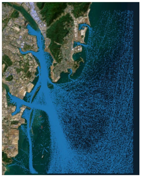
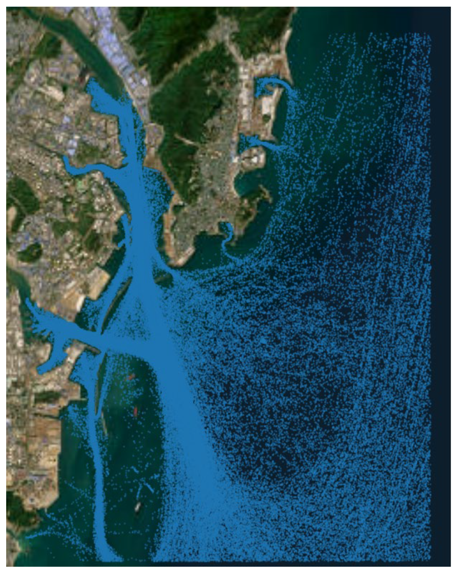
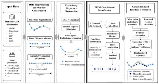
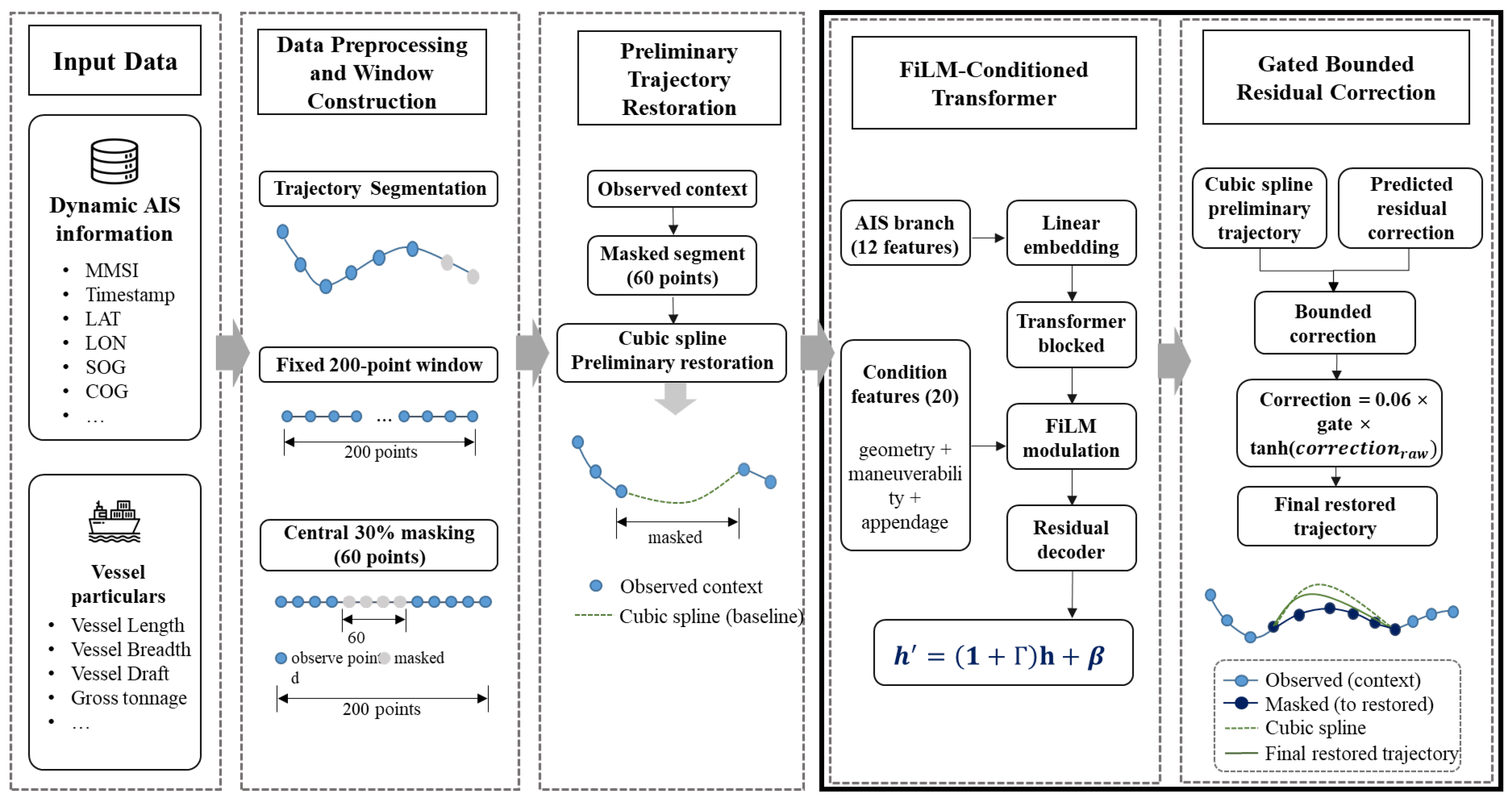
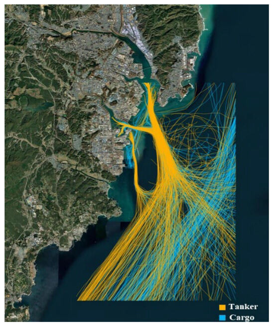
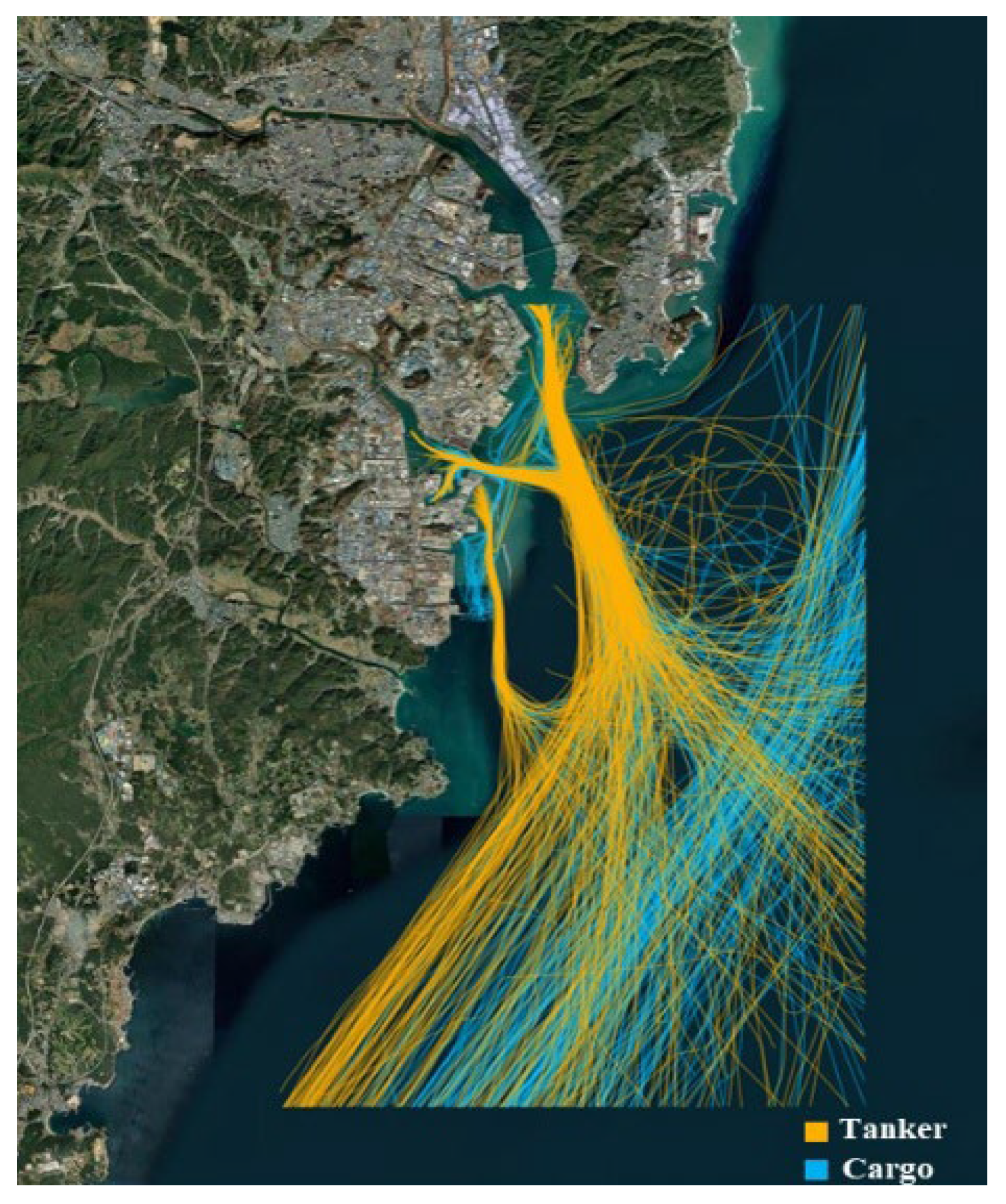
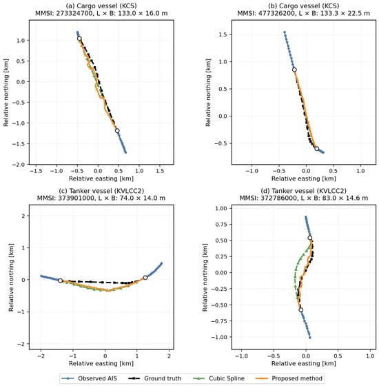
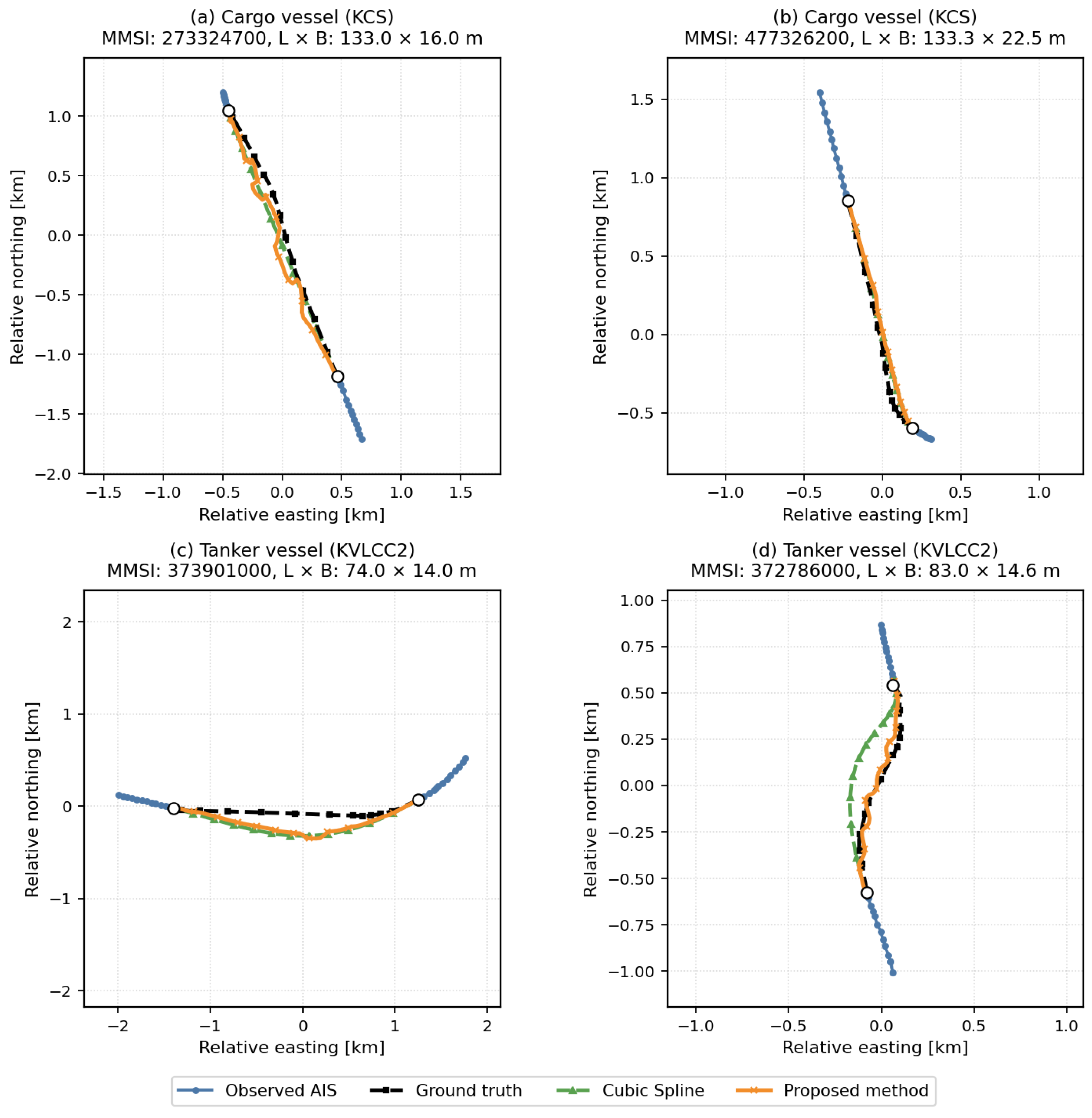

Disclaimer/Publisher’s Note: The statements, opinions and data contained in all publications are solely those of the individual author(s) and contributor(s) and not of MDPI and/or the editor(s). MDPI and/or the editor(s) disclaim responsibility for any injury to people or property resulting from any ideas, methods, instructions or products referred to in the content. |
© 2026 by the authors. Licensee MDPI, Basel, Switzerland. This article is an open access article distributed under the terms and conditions of the Creative Commons Attribution (CC BY) license.