


Abstract
Near-field underwater charging alignment requires six-degree-of-freedom (6-DoF) target pose estimates that remain geometrically stable under optical degradation while meeting onboard computational constraints. Attenuation, backscatter, non-uniform illumination, specular disturbance, and motion blur can weaken the local visual cues required for reliable monocular pose recovery. This paper presents a lightweight degradation-aware perception framework for near-field underwater charging alignment. The framework combines simplified physics-inspired underwater image synthesis, a lightweight high-resolution keypoint network, geometry-aware supervision with paired clean/degraded consistency learning, and quality-aware PnP pose recovery using underwater effective intrinsics. Evaluation includes a public 6-DoF reference benchmark, controlled low-light and motion-blur tests, the task-oriented Charging-UW dataset, and real underwater pool experiments. The controlled tests show substantially higher sensitivity to severe visibility loss than to the tested motion-blur range. In the 174-frame quantitative real-pool evaluation, the complete quality-aware pose-recovery procedure provides valid poses for all reference-valid frames, with median translation and rotation discrepancies of 3.71 cm and 3.08°, respectively, while the embedded inference pipeline operates at approximately 20 FPS on an NVIDIA Orin NX. These results demonstrate the feasibility of the proposed lightweight monocular pose-estimation framework for near-field underwater charging alignment. The present evaluation focuses on the perception stage preceding closed-loop insertion.
1. Introduction
Long-duration underwater operation increasingly depends on reliable subsea energy replenishment. Plug-in charging is attractive because it can provide direct electrical connection and high power-transfer capability for subsea infrastructure and resident robotic systems [1,2,3]. In practice, however, close-range connector operations are still commonly supported by teleoperation using work-class remotely operated vehicles (ROVs) or underwater vehicle–manipulator systems (UVMS), which limits repeatability and increases the operational burden of recurrent charging tasks [4,5].
This work addresses the visual-perception problem that precedes physical insertion: estimating the relative 6-DoF pose of a charging target during near-field alignment. The estimate is intended to serve as an upstream geometric measurement for downstream visual servoing or local alignment control. The present study does not evaluate closed-loop manipulator control, contact interaction, or physical connector insertion. This scope distinction is important because the perception module must first provide sufficiently stable translation and rotation estimates before system-level insertion performance can be meaningfully assessed.
Near-field monocular perception is particularly difficult underwater. Attenuation and scattering reduce contrast and edge strength; non-uniform illumination and specular reflections alter local appearance; suspended particles and background clutter introduce distractors; and vehicle or manipulator motion can produce blur. These effects directly degrade the 2D image evidence from which 3D pose is recovered. At the same time, onboard robotic platforms impose strict limits on model size, computation, power consumption, and latency. The resulting task is therefore an application-constrained perception problem that jointly involves degraded image formation, limited annotated data, geometric reliability, and embedded computational constraints.
Existing underwater intervention systems often reduce perceptual uncertainty through cooperative markers, engineered scene structure, favorable visibility, or additional sensing modalities [6,7,8]. Recent studies on underwater charging alignment and docking guidance further illustrate the importance of stable relative-pose perception during the near-field approach [9,10,11]. These strategies are effective when the environment can be instrumented, but they do not fully address markerless passive monocular perception of a charging target under variable optical conditions. Conversely, modern monocular 6-DoF pose-estimation methods provide strong geometric capabilities on terrestrial benchmarks, yet their computational cost and sensitivity to visual degradation can restrict direct deployment on compact underwater platforms. This motivates a perception design that preserves explicit 2D–3D geometry while incorporating degradation robustness and computational efficiency.
To address this requirement, we develop a lightweight degradation-aware monocular 6-DoF pose-estimation framework for near-field underwater charging alignment. The individual building blocks employed in the framework, including high-resolution backbones, multi-scale feature fusion, feature-wise conditioning, consistency learning, and PnP, are established techniques. The technical contribution of this work therefore does not lie in any one of these components in isolation. Instead, it lies in their task-specific coupling: degradation-aware correspondence prediction is trained together with explicit geometric and correspondence-reliability supervision, and the predicted reliability is subsequently used by the geometric pose-recovery stage to select the 2D–3D evidence supplied to PnP. This formulation preserves an explicit correspondence-to-pose chain while targeting the degradation and embedded-computation constraints of near-field underwater charging alignment. The main contributions are summarized as follows:
- We develop a simplified physics-inspired underwater image-synthesis pipeline with domain randomization for generating annotated training data. The model introduces depth-dependent attenuation and backscatter trends, backscatter noise, and a depth-conditioned blur approximation while preserving exact geometric labels. Because normalized rather than metric depth is used, the synthesis parameters are treated as effective augmentation parameters rather than calibrated optical properties of a specific water body.
- We propose LDA-KNet, a lightweight degradation-aware keypoint network built on Lite-HRNet. The network combines lightweight multi-scale fusion, a center-plus-relative-corner representation, corner-quality estimation, and degradation-context modulation to preserve geometrically meaningful 2D–3D correspondences under degraded visual conditions.
- We introduce geometry-aware supervision together with paired clean/degraded consistency learning. The training objective couples pointwise keypoint accuracy, rigid structural regularization, correspondence-quality estimation, and cross-degradation consistency so that the learned representation remains suitable for PnP-based 6-DoF recovery.
- We integrate the learned correspondence model with quality-aware robust PnP using underwater effective intrinsics and evaluate the resulting perception pipeline through a general public benchmark, controlled degradation tests, the task-oriented Charging-UW dataset, and real underwater pool sequences on an embedded NVIDIA Orin NX platform. The public benchmark is used as a general reference, whereas the principal task-oriented evidence is provided by underwater synthetic and real-pool evaluations.
The remainder of this paper is organized as follows. Section 2 reviews monocular 6-DoF pose estimation and underwater intervention perception, with emphasis on the requirements of near-field charging alignment. Section 3 presents the proposed degradation-aware geometric perception framework. Section 4 describes the public, controlled-degradation, task-oriented underwater, and real-pool experiments. Section 5 discusses the engineering implications and limitations, and Section 6 concludes the paper. Additional implementation and quantitative details are provided in the appendices.
2. Related Work
The present study lies at the intersection of monocular 6-DoF pose estimation, underwater intervention perception, and pose recovery under underwater image degradation. The first area provides the correspondence and geometric-recovery mechanisms used by the method, whereas the latter two define the deployment constraints that motivate the proposed design.
2.1. 6-DoF Pose Estimation from Monocular RGB
Monocular RGB-based 6-DoF pose estimation is commonly formulated either through explicit 2D–3D correspondences followed by geometric recovery or through denser/direct pose prediction. Keypoint-based methods predict predefined object landmarks and recover pose with PnP [12,13,14,15]. Their main advantage for manipulation-oriented perception is that image evidence, correspondence quality, reprojection error, and the final estimate remain geometrically interpretable. Their main weakness is sensitivity to inaccurate or missing keypoints under occlusion, blur, and weak texture.
Direct-regression and dense-correspondence approaches can achieve strong benchmark accuracy through more expressive prediction and refinement mechanisms [16,17,18,19]. However, additional representational capacity and refinement stages generally increase computation and implementation complexity. For underwater embedded deployment, the relevant trade-off is therefore not benchmark accuracy alone, but the balance among geometric reliability, degradation robustness, and inference cost. LINEMOD [20] is retained in this work primarily as a standard reference for general 6-DoF capability rather than as the principal task domain.
2.2. Perception for Underwater Charging Alignment and Intervention
Underwater intervention requires local geometric perception that can support closed-loop motion near a target. UVMS and work-class ROV systems have demonstrated grasping, valve operation, panel interaction, and other manipulation primitives through visual servoing and task-priority control [5,6,7]. In many systems, perception is simplified by fiducials, cooperative fixtures, structured panels, or other engineered cues. Such aids can substantially improve robustness, but they reduce the extent to which the system can rely on passive markerless perception when target appearance, viewpoint, or water conditions vary.
Charging and wet-mate connector operations are especially sensitive to relative geometry because the final approach must bring the vehicle or manipulator into a constrained local configuration before contact [9,21]. Related underwater docking and visual-guidance studies likewise emphasize reliable relative-pose or alignment estimation during terminal approach [10,11]. Beyond vision-only terminal guidance, recent underwater cooperative-positioning studies have also combined navigation and inter-vehicle ranging information to improve localization robustness in complex marine environments [22]. In this context, the perception problem considered here is near-field relative-pose estimation of the charging target for subsequent alignment control.
Recent underwater perception studies increasingly combine learned visual features with explicit geometric recovery so that the output remains an interpretable pose rather than only a detection result [23,24,25]. This formulation is well suited to manipulation-oriented tasks because confidence, reprojection residuals, calibration, and downstream coordinate transforms can be analyzed explicitly. The proposed method follows this direction while placing additional emphasis on lightweight computation and robustness to degraded monocular imagery.
2.3. Object Pose Estimation Under Underwater Image Degradation
Applying terrestrial pose-estimation methods underwater is complicated by attenuation, backscatter, color shift, low contrast, non-uniform illumination, suspended particles, and motion-induced blur. Real underwater data with accurate 6-DoF annotations are costly to acquire, so synthetic rendering and domain-transfer techniques are frequently used to expand the training distribution. DeepURL, for example, trains a keypoint-based pose estimator using rendered data and reduces appearance mismatch through unpaired image-to-image translation [23,26]. Other underwater 6-DoF pipelines combine learned detection with model-based geometric constraints to improve applicability to low-texture or structurally ambiguous targets [25].
A complementary strategy is to introduce additional sensing. Range-gated or other 3D sensors can provide explicit geometric information in turbid water and thereby reduce the ambiguity inherent in monocular RGB imagery [24]. Recent bio-inspired hydrodynamic-perception studies further demonstrate that pressure-sensor arrays can provide underwater-vehicle attitude or flow-relative motion cues when optical perception is limited [27]. Such additional sensing modalities, however, increase hardware, power, synchronization, and integration requirements. For compact underwater platforms, passive monocular sensing remains attractive if sufficient robustness can be obtained computationally.
Existing underwater keypoint-based approaches primarily address the appearance-domain gap through rendered training data, domain translation, or the addition of model-based geometric constraints. In contrast, the present work keeps the correspondence representation explicit throughout the complete pipeline and additionally learns per-correspondence reliability that is consumed by the downstream geometric solver. The distinction is therefore not the use of PnP or degradation augmentation alone, but the coupling between degradation-aware correspondence learning, geometry-aware supervision, per-corner reliability estimation, and reliability-guided pose recovery under an embedded near-field charging-alignment setting.
The gap addressed in this work is therefore specific: markerless monocular 6-DoF pose estimation for near-field underwater charging alignment must remain geometrically interpretable under image degradation while operating within embedded computational limits. We address this gap through a coordinated design that combines simplified physics-inspired synthesis, degradation-aware high-resolution keypoint prediction, geometry-aware training, correspondence-quality filtering, and PnP-based recovery with task-specific underwater calibration.
3. Methodology
This section presents the proposed monocular 6-DoF perception framework for near-field underwater charging alignment. The objective is to estimate the charging-target pose relative to the camera under optical degradation and onboard computational constraints.
The framework consists of four coupled components. First, a simplified physics-inspired underwater synthesis pipeline with domain randomization is used to generate geometrically annotated training data. Second, LDA-KNet predicts the object center, relative corner offsets, and corner-quality estimates while preserving high-resolution visual features. Third, training combines geometry-aware supervision with paired clean/degraded consistency learning. Fourth, the decoded 2D–3D correspondences are converted into a 6-DoF pose through quality-aware robust PnP using underwater effective intrinsics.
As illustrated in Figure 1, the method separates appearance learning from geometric recovery. During offline training, rendered scenes are converted into paired clean and degraded observations while their keypoint and pose annotations are retained. During online inference, LDA-KNet predicts center–corner correspondences and correspondence-quality cues from a monocular underwater frame. The final target pose is recovered by quality-aware robust PnP using the calibrated underwater effective intrinsic matrix . This separation allows the network to remain lightweight while keeping the final pose estimate tied to explicit projective geometry and reprojection-based quality indicators.
Figure 1.
Overview of the proposed framework for offline training and online pose estimation. The learned keypoint estimator is combined with underwater effective intrinsics and quality-aware geometric pose recovery to estimate the target pose required for downstream near-field alignment.
3.1. Problem Formulation
Let denote the camera coordinate frame and the charging-target coordinate frame. Given a monocular RGB image , the objective is to estimate the target pose relative to the camera,
where and . The estimated transform represents the near-field relative geometry supplied to the subsequent alignment stage.
Underwater imaging affects the problem in two distinct ways. First, optical degradation reduces the visibility and localization accuracy of image keypoints. Second, refraction introduced by the camera housing changes the effective projection geometry relative to an in-air calibration. We therefore use a decoupled formulation: the network predicts 2D geometric correspondences, while the final pose is recovered through PnP using underwater effective intrinsics calibrated for the fixed camera–housing–water configuration. This design preserves interpretability and provides reprojection residuals and correspondence statistics that can be retained as pose-quality indicators.
3.2. Physics-Inspired Underwater Image Synthesis with Domain Randomization
Collecting real images with accurate per-frame 6-DoF annotations is expensive and difficult to scale for underwater charging targets. We therefore construct a synthetic-data pipeline that combines BlenderProc 2.8.0 rendering [28] with a simplified physics-inspired degradation model. Blender 4.2.1 LTS is used as the rendering backend. The model introduces depth-dependent attenuation and backscatter trends together with stochastic backscatter variation and blur, while preserving the exact masks, keypoints, and 6-DoF annotations inherited from rendering. It is intended as a controllable training-data augmentation model rather than a full radiometric or refractive simulation of a specific water body.
Domain randomization. Within BlenderProc, we randomize camera pose, camera–object distance, viewpoint perturbation, illumination, background texture, distractor objects, and occlusion patterns. The objective is to broaden the training distribution over viewpoint, lighting, and scene clutter, thereby reducing sensitivity to distribution shift at test time.
Physics-inspired underwater degradation formulation. The synthesis procedure used to generate degraded training images with inherited pose annotations is detailed in Appendix A. For each pixel x and color channel , we use a simplified direct-transmission/backscatter decomposition inspired by classical underwater image-formation models [29,30]:
where is an effective transmittance term, is the normalized rendered depth, is an effective channel-wise synthesis coefficient, and is a background-light term. Because normalized depth is used, is not interpreted as a measured attenuation coefficient in physical units. The formulation preserves the qualitative depth dependence of attenuation and backscatter while allowing broad appearance randomization.
To approximate stochastic background variation associated with suspended particles, Gaussian noise is injected into the background term:
The degraded image with backscatter noise is then given by
Forward-scattering blur. To approximate the low-pass appearance associated with forward scattering, we use a spatially invariant Gaussian blur whose standard deviation is driven by the normalized-depth statistics:
The final channel-wise observation is therefore
To visualize how typical underwater degradation factors are progressively accumulated in the proposed pipeline, we present a “degradation ladder” from ideal rendering to the final underwater observation in Figure 2. The figure sequentially illustrates the effects of absorption/attenuation, backscatter, backscatter noise, and forward-scattering blur. This step-wise presentation provides an interpretable view of how the selected degradation factors are accumulated. The blur term should be understood as a computational surrogate for scattering-induced loss of high-frequency detail rather than as a full spatially varying scattering point-spread function.
Figure 2.
Degradation ladder from clean rendering to underwater observation: (a) clean , (b) attenuation , (c) +backscatter , (d) +backscatter noise, (e) +forward-scattering blur.
To cover typical optical differences between blue water and green water as well as a range of turbidity levels, we employ the parameter ranges listed in Table 1. These settings are used consistently in the dataset construction process.
Table 1.
Parameter ranges used by the simplified physics-inspired underwater synthesis pipeline.
The ranges in Table 1 are selected as augmentation ranges that span representative blue/green appearance changes and degradation severities; they are not claimed to be calibrated optical properties of the pool water used in the real experiments. During training, we further apply global darkening, local illumination perturbation, contrast compression, channel-wise color shifts, motion blur, and residual blur. These image-space perturbations complement the offline synthesis model by extending the range of visibility loss and local appearance variation presented to the network. Training and testing samples are generated from disjoint camera poses, background realizations, random seeds, and occluder configurations to reduce leakage between data construction and evaluation. Figure 3 provides an overview of the LDA-KNet architecture and the paired clean/degraded training scheme.
Figure 3.
Overview of the proposed LDA-KNet-based framework. Panel (A) shows the LDA-KNet architecture built upon a Lite-HRNet backbone and a lightweight bidirectional feature-pyramid network (BiFPN). Panel (B) illustrates paired clean/degraded consistency training with geometric supervision. Panel (C) details the pose-head building blocks. The network predicts the object center, relative corner offsets, and corner-quality estimates for PnP-based pose recovery.
3.3. LDA-KNet: A Lightweight Degradation-Aware Keypoint Network
Design rationale. Underwater pose estimation requires a representation that preserves fine geometric detail while keeping computation moderate. This requirement becomes more stringent under low contrast, non-uniform illumination, and motion blur, where aggressive downsampling can suppress weak local structures needed for stable correspondence estimation. We therefore adopt a lightweight high-resolution design and build LDA-KNet by augmenting Lite-HRNet with degradation-aware conditioning and lightweight multi-scale fusion.
Backbone and lightweight multi-scale fusion. LDA-KNet uses Lite-HRNet [31] as the backbone because its parallel multi-resolution branches retain high-resolution features that are useful for localizing weak geometric structures. Three backbone feature levels are channel-aligned and fused through a lightweight bidirectional feature-pyramid network (BiFPN) with top-down and bottom-up aggregation. This multi-scale fusion combines fine local geometry with higher-level context while maintaining a compact feature hierarchy.
Center-relative pose head and degradation context. The pose head predicts objectness, the 2D object center, eight corner offsets relative to that center, and a quality score for each corner. Prediction is performed on dense feature-grid locations under objectness supervision, but the geometric representation is center-relative rather than eight independent absolute image coordinates. This reduces the coordinate range that must be regressed and couples the corner predictions to a common object reference. A lightweight refinement branch operates on the highest-resolution pose feature, and the predicted corner-quality scores are subsequently used to reject unreliable 2D–3D correspondences before PnP.
A compact degradation-context representation is extracted from intermediate features and used to modulate the pose-regression features through feature-wise linear modulation (FiLM). Rather than estimating a physically calibrated degradation parameter, this branch provides a learned latent context that allows the pose features to adapt to appearance changes such as severe darkening and blur. The context representation is optimized end-to-end through the pose and cross-degradation consistency objectives.
Coordinate decoding. Let the decoded center location be denoted by . For the k-th cuboid corner, the network predicts a relative offset , and the decoded image coordinate is
The object center acts as a common geometric anchor for corner prediction rather than as an additional PnP correspondence. The downstream pose-recovery stage uses the eight decoded cuboid corners together with their predicted quality scores. During training, the center contribution is detached when constructing the corner-related regression path, while the center itself is supervised separately. This prevents accumulated corner residuals from dominating optimization of the shared center prediction.
Compared with direct independent absolute-corner regression, the center-plus-relative-offset parameterization reduces the coordinate range of the corner predictions and explicitly couples them to a common object reference.
3.4. Geometry-Aware Supervision and Paired Clean/Degraded Consistency Learning
The training objective is designed to optimize accurate image-space center–corner geometry while maintaining stable predictions across clean/degraded observations of the same underlying pose. The complete proposed configuration combines decoded corner supervision, center-relative supervision, rigid-structure regularization, correspondence-quality learning, and clean-teacher cross-degradation consistency.
3.4.1. Single-Branch Geometric Supervision
For each input image, the pose head predicts an objectness logit, a 2D object center, eight relative corner offsets, and eight corner-quality logits. The decoded corner coordinates follow Equation (7).
The single-branch geometric objective is written as
In the reported configuration, , , , and .
Decoded absolute-corner supervision. Let
denote the coordinate-averaged absolute error of the k-th decoded corner. To place additional emphasis on difficult correspondences, the two corners with the largest current localization errors are assigned twice the ordinary weight. Let denote the resulting corner weight and let denote the square-root area scale derived from the target bounding box. The decoded-corner regression term is
Here and below, denotes a small numerical constant used to avoid division by zero.
Center-anchor supervision. The 2D center is supervised independently from the corner-related path. Defining
the center-anchor term follows the same saturating regression principle used by the implementation:
When computing the corner-related losses, the decoded center is treated as a stop-gradient anchor so that corner residuals do not directly modify the center prediction.
Relative-corner supervision. Let denote the ground-truth center-to-corner offset, and let denote the mean length of the 12 ground-truth projected cuboid edges. The relative offsets are normalized by and supervised with a Smooth- loss:
This term directly supervises the relative representation used by the pose head, whereas constrains the corresponding decoded image coordinates.
Object-keypoint-similarity supervision. A scale-aware keypoint-similarity term is additionally applied to the decoded corners:
where in the reported configuration.
Objectness supervision. Objectness is optimized using binary cross-entropy with logits. Instead of assigning every positive location a unit target, the positive target is a soft geometric confidence derived from agreement between the predicted and ground-truth keypoint configurations. Background locations retain zero objectness. The objectness contribution is activated after the initial 40-epoch geometric pretraining stage.
3.4.2. Corner-Quality Supervision
For the k-th cuboid corner, let
denote its image-space localization error. A soft quality target is generated from the normalized geometric error:
The quality objective combines soft-target binary cross-entropy and a pairwise ranking constraint:
For a pair of corners , if their normalized errors satisfy
corner i is regarded as geometrically more reliable, and the predicted quality scores are encouraged to satisfy with through a hinge-ranking penalty. The quality target is detached from gradient computation, so the quality branch learns correspondence reliability without feeding its target construction back into the keypoint coordinates.
3.4.3. Rigid-Structure Regularization
Pointwise localization alone does not guarantee a globally coherent cuboid. Let , , and denote the predefined sets of cuboid edges, face diagonals, and body diagonals, respectively. For a point pair , define the predicted and ground-truth image-space vectors as
For a pair set , the normalized length and direction losses are
A corresponding center-to-corner term and is constructed from the eight center–corner vectors. The rigid-structure objective used in the reported model is
Together, these terms constrain both local pairwise geometry and long-range center–corner consistency while remaining normalized with respect to the projected target scale.
3.4.4. Paired Clean/Degraded Consistency Learning
For each training pose, a clean observation and a degraded counterpart share the same geometric annotation. Ordinary single-branch supervision is applied to both observations. In addition, the clean branch acts as a stop-gradient teacher for the degraded branch.
For keypoint consistency, the decoded clean center and clean relative corner offsets are detached and used as teacher targets:
where denotes stop-gradient and collects the eight relative corner offsets.
For quality consistency, the clean quality probabilities are used as soft teacher targets:
Only teacher correspondences satisfying participate in the quality-consistency loss, which is implemented as binary cross-entropy between the degraded quality logits and the clean teacher probabilities.
Both consistency terms are further weighted according to degradation severity. Let denote the maximum recorded degradation severity of sample i; its consistency weight is
The per-sample contributions to both and are multiplied by before minibatch averaging. The cross-degradation objective is therefore
with
3.4.5. Total Training Objective
For the single-class pose-estimation setting considered in this work, the single-branch objective combines the geometric correspondence objective with objectness supervision:
where denotes the indicator function and . The classification loss is inactive in the single-class setting. Hence, the initial training stage emphasizes geometric center–corner learning, while objectness supervision is introduced after the 40-epoch geometric pretraining stage.
Let and denote the resulting single-branch objectives for the paired clean and degraded observations, respectively. The complete objective is
where progressively activates the cross-degradation consistency terms:
Thus, the first 40 epochs emphasize single-image geometric learning. Objectness and paired clean/degraded consistency are subsequently introduced, with the consistency contribution linearly increased to its full weight by epoch 60.
3.5. Quality-Aware Pose Recovery
Native-coordinate recovery and underwater effective intrinsics. LDA-KNet operates entirely in the 2D image domain and does not require camera intrinsics during network training. During inference, the network processes letterboxed images. Before metric pose recovery, the predicted cuboid corners are mapped from the network-input coordinate system back to the native image coordinate system using the recorded resize gain and padding. The corresponding ground-truth keypoints are transformed in the same way during evaluation.
Because the water–housing–air optical path modifies the effective projection geometry relative to an in-air calibration [32,33,34], the camera is calibrated underwater using the same housing configuration as the deployment system. Calibration-board observations are collected over multiple poses and working distances, and standard Zhang calibration [35], followed by nonlinear reprojection-error minimization, is used to estimate the effective projection parameters. The resulting underwater effective intrinsic matrix is
This matrix is treated as a task-specific effective-pinhole approximation for the fixed camera–housing configuration and the tested near-field operating envelope. The formulation is not intended to represent the complete physical refraction of the water–housing–air imaging path. Flat-port underwater imaging is generally not exactly central, and explicit refractive camera models can provide higher geometric fidelity when wider viewing angles, larger working ranges, or stricter metric-accuracy requirements are considered [32,33,34]. In the present work, underwater calibration is therefore used as a practical task-specific projection approximation rather than introduced as a new refractive-calibration contribution. Although conventional lens-distortion coefficients are also obtained during calibration, they are not explicitly included in the reported PnP stage. The numerical values of used in the real-pool experiments are reported in Appendix B (Table A1).
Quality-aware correspondence selection and robust PnP. Let denote the eight predefined 3D cuboid corners and let denote the corresponding predicted 2D corners after inverse-letterbox mapping to the native image coordinate system. Their predicted correspondence-quality scores are denoted by . The predicted object center remains a network anchor and is not used as a PnP correspondence. Figure 4 summarizes the quality-aware pose-recovery procedure.
Figure 4.
Quality-aware pose recovery. Predicted cuboid corners are selected according to correspondence quality and spatial diversity for pose initialization, followed by residual- and quality-aware refinement using all eight corners. The initialization uses RANSAC-PnP with a predefined EPnP + LM fallback when a valid RANSAC solution is unavailable. The predicted object center is used only as a network anchor and is excluded from the PnP correspondences.
We first construct a geometrically diverse high-quality subset . The highest-quality corner is selected first, after which additional corners are chosen greedily according to
where denotes the minimum image-space distance from candidate k to the already selected corners and is the diagonal extent of the predicted corner configuration. Exactly six correspondences are retained for pose initialization.
An initial pose is estimated using RANSAC-based PnP with a 3-pixel reprojection threshold, followed by nonlinear refinement:
If RANSAC does not return a valid pose, the implementation uses the predefined fallback consisting of ordinary EPnP on the same selected correspondences followed by Levenberg–Marquardt (LM) refinement. No correspondence-selection or PnP parameter is changed by this fallback.
Starting from this pose, all eight corners are reconsidered through a quality- and residual-aware refinement procedure. For each corner, the reprojection residual is
where denotes perspective division.
Corners satisfying either pixels or are retained. If fewer than six correspondences satisfy these conditions, the remaining candidates are ranked according to
and the highest-ranked corners are added until six correspondences are available. The pose is subsequently refined without RANSAC, and this residual-based refinement is repeated for at most two iterations.
These values are treated as fixed engineering hyperparameters rather than theoretically optimal constants. The spatial-diversity term is normalized by the diagonal extent of the predicted corner configuration, so controls the trade-off between learned correspondence quality and spatial spread without introducing an additional image-scale unit. The 3-pixel threshold defines the native-image reprojection-consistency criterion, whereas the high-quality condition allows a correspondence with strong learned reliability to remain eligible during re-selection. Six correspondences are retained for initialization so that the selected set remains overdetermined relative to minimal PnP while allowing two of the eight predicted corners to be excluded. These hyperparameters are fixed throughout the reported real-water evaluation and are not adjusted according to the resulting pose errors or success rates. The resulting refined pose is taken as the final estimate .
4. Experiments
The experimental evaluation is organized as a progressive validation chain from general pose-estimation capability to task-specific underwater deployment. First, LINEMOD is used only as a standard terrestrial reference to establish general 6-DoF pose-estimation capability and to facilitate comparison with representative prior methods. Second, controlled low-light/darkness and motion-blur experiments are used to characterize the failure envelope of the proposed model under isolated visual degradations. Third, Charging-UW provides a task-oriented synthetic intermediate domain in which multiple underwater appearance degradations, clutter, and occlusion are combined under controlled ground-truth pose annotations. Finally, the method is evaluated in real underwater pool experiments, where geometric accuracy and temporal stability are assessed using a ChArUco-derived reference pose. Embedded execution on an NVIDIA Orin NX is reported separately as the deployment-side efficiency evidence.
4.1. Datasets and Evaluation Settings
Two benchmark datasets are used for the dataset-based quantitative evaluations. LINEMOD provides a standard non-underwater reference for general 6-DoF pose estimation, whereas Charging-UW is used as a task-oriented synthetic intermediate domain between the controlled degradation tests and real-water validation. The real underwater manipulator acquisitions used for near-field quantitative evaluation are described separately in Section 4.4.5.
4.1.1. LINEMOD as a General 6-DoF Reference
We use the public LINEMOD dataset [20] as a general-reference benchmark rather than as the principal application domain of this study. The dataset contains 13 representative rigid objects with cluttered backgrounds, frequent occlusions, and illumination variations. Each scene may contain multiple objects, while a 6-DoF pose annotation is provided for the target object.
The dataset covers objects with different geometry, texture, symmetry, and specularity, making it useful for verifying that the proposed lightweight representation retains general pose-estimation capability outside the underwater domain.
We follow the commonly adopted LINEMOD training/testing split and evaluation protocol to maintain comparability with prior work. Each object category contains approximately 1200 images. The standard split is used such that the minimum angular distance between test poses is approximately , with about of samples used for training and for testing. ADD-S is used for symmetric objects such as Eggbox and Glue, whereas ADD is used for the remaining objects.
4.1.2. Charging-UW as a Task-Oriented Synthetic Intermediate Domain
We construct a task-oriented synthetic dataset, termed Charging-UW, using BlenderProc [28] together with the simplified physics-inspired underwater synthesis procedure introduced in Section 3.2. Charging-UW contains 3300 images, including 2640 training images and 660 testing images, at a native resolution of . Each sample includes RGB data, depth, an object mask, and 6-DoF pose annotations in the BOP format [36]. The target is the charging-alignment object shown in Figure 5, and distractor objects are sampled from the BOP object pool to increase background complexity and partial occlusion. The charging-target CAD geometry does not exhibit exact geometric symmetry; ordinary ADD is therefore used as the primary model-space pose metric for both the cross-method Charging-UW comparison and the controlled component ablation.
Figure 5.
Target used for the task-oriented underwater evaluation. (a) Near-field underwater charging target used in this work. (b) Corresponding CAD model used for rendering and geometric pose recovery.
Scene and pose sampling protocol. Camera viewpoints are sampled in spherical coordinates centered on the target, with azimuth in , camera–target distance in m, and an additional perturbation of the optical axis. Illumination, background texture, distractor count, and occlusion are randomized to increase variation in viewpoint, lighting, and scene clutter.
Synthetic underwater degradation. Charging-UW uses the same simplified physics-inspired degradation formulation and parameter ranges introduced in Section 3.2 and Table 1. The corresponding degradation ladder is shown in Figure 2. As discussed in the methodology, this formulation is used as a controllable augmentation and data-generation model; its effective degradation parameters are not interpreted as calibrated optical properties of the water used in the real pool experiments.
Training and testing samples are generated using disjoint camera poses, background realizations, random seeds, and occluder configurations. Charging-UW therefore serves as a controlled intermediate domain for evaluating compound underwater appearance degradation before testing the method on real underwater imagery. It is not treated as a substitute for real-water validation.
4.2. Evaluation Metrics
Different metrics are used according to the purpose of each validation stage. LINEMOD is evaluated using the conventional ADD/ADD-S protocol. Charging-UW is evaluated using MCE, 2D reprojection accuracy, threshold-based pose accuracy, translation and rotation errors, and ordinary ADD as the primary model-space pose metric for the cross-method and component-ablation evaluations. The real underwater evaluation distinguishes between ROV-mounted longer-range qualitative trials and manipulator-based near-field quantitative trials. The qualitative trials are used only to assess visual transfer and geometric coherence and are not included in the pose-error statistics. For the near-field quantitative evaluation, pose validity is computed over the complete reference-valid cohort of each acquisition. Because method-specific detection failures can produce different valid subsets, continuous cross-method translation and rotation discrepancies are compared on the exact common-valid frame subset for each acquisition. The joint 5 cm/ criterion is evaluated over the complete reference-valid cohort, with invalid method outputs counted as failures. Accuracy statistics are reported separately for the different near-field acquisitions rather than pooled across them.
Mean corner error. For Charging-UW, mean corner error (MCE) measures the image-space localization accuracy of the eight projected cuboid corners:
where and denote the predicted and ground-truth image coordinates of the k-th cuboid corner, respectively. The object-center prediction is not included in MCE.
ADD/ADD-S. Let M denote the set of 3D model points, the reference pose, and the estimated pose. ADD is defined as
For symmetric objects, ADD-S is computed using the nearest-point distance:
On LINEMOD, ADD-S is used for Eggbox and Glue, whereas ADD is used for the remaining objects. The conventional 10% ADD/ADD-S(*) criterion reports the percentage of test poses whose model-point error is below 10% of the corresponding object diameter.
For the Charging-UW cross-method comparison and the controlled component ablation, the charging-target CAD model does not exhibit exact geometric symmetry. Ordinary ADD is therefore used as the model-space pose metric in both evaluations. The model diameter is defined as the maximum pairwise Euclidean distance between CAD vertices, yielding m. An estimated pose is counted as successful when
This gives a common ADD threshold of approximately m. The ADD success rate is computed over the complete 660-image test set, with samples without a valid recovered pose counted as failures.
2D reprojection and threshold-based pose metrics. For Charging-UW, the 2D projection metric is evaluated from the projected CAD-model geometry, and Proj@5px reports the fraction of test samples satisfying the adopted 5-pixel projection-error threshold. We additionally retain the 5 cm/ pose-success threshold to provide a common scalar comparison between methods.
The 5 cm/ criterion is used solely as a threshold-based pose-estimation metric for method comparison. It is independent of the connector-specific mechanical tolerances that govern physical insertion.
Translation and rotation errors. For an estimated pose and a reference pose , the translation error is
and the rotation error is evaluated using the geodesic distance on :
These metrics retain direct interpretations in translation and orientation space and are used for both Charging-UW and the quantitative real-pool evaluation.
Model complexity and runtime. Model complexity is characterized using the number of trainable parameters and FLOPs. Benchmark-side runtime values are reported as indicative comparisons with prior methods. Unless otherwise specified, these timings correspond to batch size 1 and the timing convention used in the associated benchmark implementation. Deployment-side runtime is evaluated separately on an NVIDIA Orin NX configured for onboard execution of the complete perception pipeline. This directly measured embedded throughput, rather than the benchmark-side reference estimate, is used as the primary evidence of onboard computational feasibility.
4.3. Implementation Details
The training implementation uses Python 3.9.25 and PyTorch 1.13.1+cu117. The proposed network is trained from scratch on a single NVIDIA RTX 3090 GPU (NVIDIA Corporation, Santa Clara, CA, USA) for 1500 epochs with a batch size of 12. Adam is used with , , an initial learning rate of , and a base weight decay of . The learning rate follows a cosine-shaped decay with a final learning-rate factor of 0.01. A nominal 3-epoch optimizer warm-up is configured, with a minimum of 1000 warm-up iterations, an initial warm-up momentum of 0.8, and a warm-up bias learning rate of 0.1. A fixed random seed of 1 is used for the reported single-GPU experiments. The final-epoch checkpoint is retained for the reported evaluation to avoid test-set-driven checkpoint selection.
The native Charging-UW images have a resolution of and are square-letterboxed to for training and network inference. The same geometric preprocessing is applied to the associated 2D keypoint annotations. Camera intrinsics are not part of the network training objective. During metric pose recovery, the decoded keypoints are mapped back to the native image coordinate system before application of the underwater effective intrinsic matrix.
In addition to standard geometric and appearance augmentation, the training pipeline applies explicit underwater-relevant image degradation. The geometric augmentation range includes rotations up to , translation up to 0.2 of the image extent, and scale perturbation of 0.2. Additional augmentation includes color variation, illumination degradation, ordinary blur, motion blur, background replacement, and partial occlusion. Multi-scale training is disabled in the reported configuration so that the network input remains fixed at .
The initial 40 epochs emphasize geometric keypoint learning. Objectness is introduced from epoch 40 onward. Paired clean/degraded consistency is also activated at epoch 40 and linearly ramped to its full weight by epoch 60. For the reported configuration, the effective cross-degradation weights are for center/relative-keypoint consistency and for corner-quality consistency.
The principal geometric-loss hyperparameters are , , , and . The quality-target scale is . The rigid-structure weights for edge length, edge direction, face diagonal, body diagonal, and center-to-corner constraints are 0.008, 0.005, 0.005, 0.005, and 0.008, respectively. For hard-corner emphasis, the two corners with the largest current localization errors receive twice the ordinary point weight. The detector-level geometric and objectness scaling factors and follow the common training configuration and are normalized consistently across prediction levels; the same scaling rule is applied to all reported variants.
Each component-ablation variant is trained independently from random initialization using the same data split, optimization settings, training duration, and checkpoint-selection rule. This controlled protocol ensures that the comparisons in Section 4.4.4 reflect the tested architectural and training blocks under a common optimization protocol.
Inference consists of LDA-KNet prediction, confidence-based detection filtering, inverse-letterbox coordinate recovery, and PnP-based 6-DoF pose estimation. On LINEMOD, the general-reference comparison includes YOLO6D [14], PoseCNN [16], PVNet [37], Gen6D [38], EfficientPose [39], and YOLOv5-6D [40]. On Charging-UW, YOLOv5-6D is retained as the primary reference model under the same synthetic evaluation setting. For the manipulator-based near-field real-water comparison, the same pretrained YOLOv5-6D checkpoint and inference configuration are applied to all quantitative acquisitions without pool-specific fine-tuning, checkpoint selection, threshold tuning, or pose correction. YOLOv5-6D and the complete proposed pipeline use the same underwater effective intrinsics, CAD model, and ChArUco-derived experimental reference poses. The primary cross-method comparison therefore evaluates the complete YOLOv5-6D pipeline against the complete proposed pose-recovery pipeline.
4.4. Results
The results are presented in increasing order of application specificity. Section 4.4.1 first establishes a general terrestrial reference. Section 4.4.2 then characterizes sensitivity to isolated low-light/darkness and motion-blur degradation. This is followed by the task-oriented Charging-UW evaluation in Section 4.4.3, together with the controlled component ablation in Section 4.4.4. The real underwater pool experiments in Section 4.4.5 constitute the principal real-domain validation. Finally, Section 4.4.6 reports the measured embedded execution performance on the NVIDIA Orin NX.
4.4.1. General-Reference Evaluation on LINEMOD
The purpose of the LINEMOD experiment is to establish a standard general-reference point for the proposed lightweight pose-estimation architecture. It is not used as the primary evidence for underwater charging alignment.
As shown in Table 2, the proposed method achieves an average 10% ADD/ADD-S(*) score of 82.19% across the 13 LINEMOD objects. The score is below those of several larger terrestrial methods, particularly EfficientPose and YOLOv5-6D. At the same time, high scores are retained on geometrically regular or structurally distinctive objects such as Benchvise, Eggbox, Glue, Iron, and Lamp.
Table 2.
General-reference comparison on LINEMOD using the conventional 10% ADD/ADD-S metric (%). The superscript asterisk (*) denotes symmetric objects (Eggbox and Glue), for which ADD-S is used; ADD is used for the remaining objects. The purpose of this experiment is to establish comparability with representative terrestrial 6-DoF pose estimators rather than to define the principal application benchmark of this work.
The LINEMOD results establish the general terrestrial 6-DoF capability of the lightweight high-resolution formulation. The subsequent experiments focus on degradation behavior and task-oriented underwater validation.
Table 3 provides an indicative inference-time comparison under the timing conventions of the corresponding implementations.
Table 3.
Indicative inference-time comparison on the LINEMOD cat sequence. The reported values follow the timing conventions of the corresponding implementations and may reflect different hardware and evaluation settings.
4.4.2. Failure-Envelope Analysis Under Controlled Degradation
After establishing general 6-DoF pose-estimation capability on LINEMOD, we use controlled degradation experiments to characterize the conditions under which the current visual estimator begins to lose reliable geometric information. These tests are not intended to reproduce the complete underwater image-formation process. Instead, they independently vary two practically relevant corruption families: low-light/darkness and motion blur.
Six representative LINEMOD objects are evaluated over progressively increasing degradation levels. The exact corruption operators are defined in Appendix C, and the level parameters are listed in Table A2. The average response across the six objects is summarized in Figure 6, while the complete object-wise level results are reported in Table A3 and Table A4.
Figure 6.
Failure-envelope characterization using the average 10% ADD/ADD-S(*) score over six representative LINEMOD objects. (a) Controlled low-light/darkness degradation. (b) Controlled motion-blur degradation. Shaded regions denote ±1 standard deviation across the six objects.
A clear difference appears between the two degradation families. As shown in Figure 6a, pose-estimation accuracy remains comparatively stable under low-to-moderate darkening but deteriorates rapidly once visibility becomes severely reduced. The detailed results in Table A3 show that the onset and severity of this degradation vary among objects, indicating that visible scale, geometric structure, and remaining local image evidence influence the failure point.
By contrast, the average motion-blur curve in Figure 6b remains comparatively stable over the tested range. The corresponding level-wise values in Table A4 show only moderate changes for most evaluated objects.
Under the specific darkening and motion-blur parameter ranges defined in Appendix C, the final estimator exhibits a substantially larger performance reduction under severe darkening than under the tested motion-blur settings. Because the two corruption families use different severity parameterizations, their numerical level indices are not interpreted as perceptually or physically equivalent. These experiments therefore characterize the failure envelope of the complete estimator within the tested corruption ranges rather than establish a universal ordering between low-light and motion-blur severity. This observation motivates the subsequent Charging-UW evaluation, where multiple appearance degradations, clutter, and occlusion are combined within a task-oriented underwater domain.
4.4.3. Task-Oriented Intermediate Validation on Charging-UW
The Charging-UW evaluation moves from isolated degradation factors to a compound synthetic underwater domain. The dataset combines low contrast, color shift, edge blurring, randomized illumination, scene clutter, distractor objects, and occlusion while retaining exact simulated pose annotations. Charging-UW is therefore used as an intermediate validation stage between the controlled failure-envelope experiments and the real underwater pool evaluation.
YOLOv5-6D is used as the primary reference model under the same Charging-UW evaluation protocol. EfficientPose () is additionally included as a lightweight reference to provide complementary context for the accuracy–efficiency comparison. Representative qualitative comparisons on Charging-UW are shown in Figure 7.
Figure 7.
Representative results on Charging-UW. (Top row): YOLOv5-6D reference. (Bottom row): proposed method. Green 3D bounding boxes denote simulated ground-truth poses, and blue boxes denote the estimated poses.
For the proposed method, the Charging-UW accuracy metrics reported in Table 4 are computed using the same fixed eight-corner geometric evaluator adopted in the controlled component ablation. All eight predicted cuboid corners are passed to the common PnP procedure without quality-based correspondence selection or the deployment-specific robust initialization described in Section 3.5. This separation keeps the benchmark comparison focused on the learned correspondence model and avoids confounding network accuracy with deployment-oriented geometric post-processing. The quality-aware PnP procedure is retained for the complete underwater perception pipeline.
Table 4.
Quantitative comparison on the Charging-UW synthetic intermediate domain. All threshold-based success rates are computed over the complete 660-image test set, with samples without a valid recovered pose retained in the denominator and counted as failures. Ordinary ADD is used as the model-space pose metric because the charging-target CAD model does not exhibit exact geometric symmetry. The 5 cm/ column is retained only as a common threshold-based pose-estimation metric and does not represent the mechanical tolerance required for physical connector insertion.
Table 4 shows that the proposed method and the reference methods exhibit different geometric accuracy–efficiency trade-offs on the compound underwater domain.
Under the unified 660-image evaluation protocol, YOLOv5-6D achieves an MCE of 3.28 pixels, a Proj@5px rate of 94.70%, a Pose@5cm/5° rate of 94.39%, mean translation and rotation errors of 0.011 m and 2.29°, and an ordinary-ADD success rate of 93.94%. The corresponding values of the proposed method are 3.92 pixels, 92.73%, 93.03%, 0.014 m, 3.04°, and 93.18%, respectively. EfficientPose yields an ordinary-ADD success rate of 44.55% under the same criterion. The unified comparison therefore does not indicate uniform accuracy dominance by the proposed method and is better interpreted as an accuracy–efficiency trade-off under the task-oriented Charging-UW protocol.
The proposed formulation also remains substantially more compact than the YOLOv5-6D reference, using 8.71 M trainable parameters compared with 116.67 M. The reported computational cost is 80.65 G FLOPs compared with 236.95 G FLOPs for the YOLOv5-6D reference under their respective profiling configurations. These results support the intended accuracy–efficiency balance of the proposed pose-estimation framework and motivate the embedded deployment evaluation reported later in Section 4.4.6.
The aggregate Charging-UW comparison evaluates the complete proposed configuration but does not by itself determine how the individual architectural and training components contribute to the final result. A controlled seven-variant fine-grained ablation is therefore reported next to separately examine lightweight multi-scale fusion, the center-relative/quality-aware correspondence formulation, rigid-structure regularization, degradation-context FiLM modulation, and cross-degradation consistency under the same fixed training and evaluation settings.
4.4.4. Component Ablation Study
To examine the contribution of the principal architectural and training components more explicitly, we conduct a controlled seven-variant fine-grained ablation on Charging-UW. All variants share the same Lite-HRNet backbone, local refinement branch, training data, paired clean/degraded supervised exposure, augmentation, optimization protocol, and evaluation procedure. A0 uses the absolute-corner baseline, and A1 adds lightweight BiFPN. G2 further introduces the center-relative corner representation and corner-quality supervision while leaving rigid-structure regularization disabled. A2 adds rigid-structure regularization to G2. Starting from A2, D1 activates degradation-context FiLM modulation without cross-degradation consistency, whereas C1 activates clean-teacher keypoint/quality consistency without degradation-context FiLM modulation. The Full model activates both degradation-aware mechanisms. The seven evaluated variants and their quantitative results are summarized in Table 5.
Table 5.
Fine-grained seven-variant component ablation of the proposed RGB-based 6-DoF pose-estimation framework on Charging-UW. Rel. + Q. denotes the center-relative corner representation together with corner-quality supervision; Rigid denotes rigid-structure regularization; Deg. denotes degradation-context conditioning with FiLM modulation; and Cons. denotes clean-teacher cross-degradation keypoint/quality consistency. is the number of valid recovered poses used for the continuous pose-error statistics. Proj@5px, Pose@5cm/5°, and ordinary ADD use the complete 660-image denominator, with invalid poses counted as failures. ADD is evaluated using the ordinary corresponding-point criterion at , with m.
All variants are trained independently from scratch using the same fixed 1500-epoch training protocol described in Section 4.3, and the final-epoch checkpoint is retained for evaluation. All variants are evaluated on the complete 660-image Charging-UW test set. Paired clean/degraded ordinary supervision is retained in every variant; “Cons.” therefore denotes only the additional cross-degradation keypoint/quality consistency terms.
For the controlled ablation evaluator, all eight canonical cuboid corners are passed to EPnP followed by Levenberg–Marquardt (LM) refinement. RANSAC, learned-quality correspondence gating, six-correspondence selection, residual-based re-selection, and the P2/P3 pose-recovery procedures are disabled so that all variants share the same fixed geometric post-processing procedure. Proj@5px, Pose@5cm/5°, and ordinary ADD are computed over the complete 660-image test set, with invalid poses counted as failures. The continuous translation and rotation errors are averaged over the valid recovered-pose subset. Ordinary ADD is evaluated at , where m. This fixed evaluator is used only for controlled component attribution; the complete inference pipeline uses the quality-aware initialization and residual-based refinement described in Section 3.5.
The comparison between A0 and A1 is designed to isolate the addition of lightweight bidirectional multi-scale fusion. Adding BiFPN reduces MCE from 7.10 to 5.44 pixels and reduces the mean translation and rotation errors from 0.034 m and 5.64° to 0.024 m and 4.41°, respectively. Proj@5px increases from 88.94% to 89.55%, whereas Pose@5cm/5° remains essentially unchanged (88.48% versus 88.33%). Ordinary ADD changes only slightly, from 88.94% to 89.09%. Thus, the main observed effect associated with BiFPN is reflected in the continuous keypoint and pose-error measures.
The G2 and A2 variants further decompose the original geometry-aware block by separating rigid-structure regularization from the coupled center-relative/quality-aware correspondence formulation. Comparing G2 with A1 evaluates the coupled center-relative corner representation and corner-quality supervision without rigid-structure regularization. This modification does not produce a monotonic gain: MCE increases from 5.44 to 6.47 pixels, while the translation and rotation errors increase from 0.024 m and 4.41° to 0.029 m and 5.00°, respectively. The comparison between G2 and A2 then assesses the additional rigid-structure regularization term. Proj@5px increases slightly from 88.79% to 88.94%, but the remaining reported pose metrics do not improve. We therefore do not interpret either the coupled relative/quality formulation or rigid-structure regularization as an independently additive accuracy term. The observed non-monotonic behavior indicates a trade-off among jointly optimized objectives under the present compact-model training protocol; the current ablation does not identify a unique causal mechanism for this trade-off.
D1 and C1 are sibling variants constructed from the common A2 configuration to separately assess the two degradation-aware mechanisms. Relative to A2, D1 activates degradation-context FiLM modulation while leaving cross-degradation consistency disabled. Under this comparison, MCE decreases from 6.52 to 5.99 pixels, Proj@5px increases from 88.94% to 89.09%, Pose@5cm/5° increases from 87.27% to 88.03%, and the translation and rotation errors decrease from 0.034 m and 5.34° to 0.030 m and 5.05°, respectively. The ordinary ADD rate also increases slightly from 88.48% to 88.64%.
By contrast, C1 activates the clean-teacher cross-degradation keypoint/quality consistency mechanism while leaving degradation-context FiLM modulation disabled. Relative to A2, C1 reduces the translation error to 0.027 m and increases Pose@5cm/5° and ordinary ADD to 87.73% and 89.24%, respectively, whereas MCE and Proj@5px do not improve.
The Full configuration combines degradation-context modulation and cross-degradation consistency. It does not dominate every individual metric: A1 retains the lowest MCE and rotation error and the highest Proj@5px rate. However, Full attains the highest Pose@5cm/5° rate (88.64%) and ties C1 for the highest ordinary ADD rate (89.24%). Relative to A2, Full reduces the mean translation error from 0.034 m to 0.024 m, reduces the rotation error from 5.34° to 5.06°, and increases Pose@5cm/5° by 1.36 percentage points. Compared with D1, adding consistency further improves the thresholded pose and ADD rates and reduces translation error, although MCE increases. Compared with C1, adding degradation-context modulation improves MCE, projection success, pose success, and both continuous pose errors, while the ADD rate remains unchanged. Overall, the expanded ablation shows that the proposed components interact in a metric-dependent and non-additive manner rather than forming a sequence of independently monotonic improvements.
4.4.5. Real Underwater Pool Validation
The real-water validation comprises two complementary configurations: ROV-mounted longer-range trials for qualitative transfer assessment and manipulator-based near-field trials for quantitative pose evaluation. The two are analyzed separately, and the ROV trials are excluded from the near-field quantitative statistics.
ROV-mounted longer-range qualitative evaluation.
The ROV-mounted trials assess qualitative transfer at longer stand-off distances and under representative visual interference, including target-scale variation, partial occlusion, and specular disturbance.
As shown in Figure 8, the predicted keypoints and projected target geometry remain qualitatively coherent across the tested observations, providing visual evidence of transfer to real underwater imagery.
Figure 8.
Qualitative ROV-mounted real-water evaluation at longer working distances. Panels (a–c) show representative observations at different stand-off distances, whereas panels (d–f) illustrate more challenging visual interference including partial occlusion and specular disturbance. The panels show the underwater observation, predicted keypoints, and projected 3D target geometry. Blue wireframes denote the projected 3D target bounding boxes obtained from the estimated poses, and colored point markers denote the predicted keypoints. These ROV trials are used for qualitative assessment only and are not included in the near-field quantitative pose-error statistics.
Manipulator-based near-field quantitative evaluation.
Quantitative pose accuracy is evaluated using three manipulator-based near-field acquisitions collected during the same pool-test session with an unchanged camera–target configuration. The primary acquisition contains 174 reference-valid frames collected in six sequences, a second acquisition provides 117-frame same-session replication, and a third contains 116 frames with visually evident partial-occlusion-like interference. The latter was not designed as a controlled occlusion experiment; therefore, no occlusion-severity labels or causal attribution are introduced. Accuracy is reported separately for the three acquisitions rather than pooled. The ChArUco board serves only as an engineered experimental reference for the quantitative evaluation.
Reference-pose construction.
Because independent per-frame underwater motion-capture ground truth is unavailable, quantitative evaluation uses a ChArUco-derived experimental reference. The rigidly mounted board uses the DICT_5X5_100 dictionary, with 0.04 m squares and 0.03 m markers. Let , , and denote the camera, board, and charging-target frames, respectively.
Their fixed relative pose is represented by the full board-to-target rigid-body transformation
The fixed full- board-to-target transform was estimated independently from a separate 27-frame calibration acquisition using target landmarks with known CAD-frame coordinates and was frozen before quantitative evaluation. Network predictions and evaluation frames were not used in this calibration. The joint fit yields a landmark reprojection RMS of 1.27 px, while a five-fold recalibration check gives P95 transform changes of 0.32 mm in translation and 0.054° in rotation. These quantities characterize the stability of and are distinct from the camera intrinsic calibration reported in Appendix B.
All three near-field acquisitions use the same camera–housing configuration, target, ChArUco fixture, CAD model, underwater effective intrinsic matrix, and fixed . For each frame, interpolated ChArUco corners are refined to subpixel accuracy and the board pose is estimated independently using the same effective-pinhole intrinsic matrix and zero conventional distortion coefficients as the model-side PnP stage.
The resulting per-frame board pose relative to the underwater camera is denoted by . The corresponding reference pose of the charging target is obtained through the fixed rigid-body transformation
Valid ChArUco reference poses are available for all 174 frames in the primary near-field evaluation, all 117 frames in the same-session replication acquisition, and all 116 frames in the partial-occlusion-like acquisition.
The ChArUco-derived pose is treated as an experimental reference rather than independent metrology-grade ground truth. Using the same effective-pinhole projection convention removes differential model bias between the two evaluation paths but does not remove common-mode calibration or approximation error; the reported pool results are therefore estimator-to-reference discrepancies.
Full-pipeline near-field comparison.
The complete proposed pipeline and a frozen YOLOv5-6D baseline are evaluated on the same three near-field acquisitions using the same calibrated camera model, CAD geometry, and ChArUco-derived experimental reference. No real-pool image is used for training, checkpoint selection, synthesis tuning, or pool-specific fine-tuning, and no post-result parameter adjustment is performed. Figure 9 shows representative full-pipeline overlays selected from predefined temporal positions independently of pose error or method success.
Figure 9.
Representative full-pipeline comparisons in the manipulator-based near-field real-water evaluation. (a) Primary acquisition, first predefined temporal sample; (b) same-session replication acquisition, first predefined temporal sample; (c) supplementary acquisition containing visually evident partial-occlusion-like interference, first predefined temporal sample; (d) primary acquisition, second predefined temporal sample; (e) same-session replication acquisition, second predefined temporal sample; (f) supplementary acquisition containing visually evident partial-occlusion-like interference, second predefined temporal sample. Orange, cyan, and blue denote the ChArUco-derived experimental reference, YOLOv5-6D, and the complete proposed method, respectively. Per-frame translation and rotation discrepancies relative to the same experimental reference are reported below each panel. When YOLOv5-6D does not provide a valid detection, the corresponding panel is marked as “No detection”. Frame selection is independent of pose error and method success.
Table 6 shows acquisition-dependent differences. The proposed method maintains full pose availability in all three acquisitions, whereas YOLOv5-6D is particularly limited in the replication acquisition (41/117 valid poses). On the exact common-valid subsets, the proposed method also exhibits smaller upper-tail translation and rotation discrepancies. The partial-occlusion-like result is interpreted descriptively because that acquisition was not designed as a controlled single-factor occlusion study.
Table 6.
Full -pipeline comparison across the manipulator-based near-field real-water acquisitions. Pose validity and the 5 cm/ success rate are evaluated over the complete reference-valid cohort of each acquisition, with invalid outputs counted as failures for the threshold metric. Continuous translation and rotation errors are evaluated on the exact common-valid subsets, containing 91, 41, and 115 frames for the primary, replication, and partial-occlusion-like conditions, respectively. No accuracy metric is pooled across acquisitions.
Pose-recovery ablation on the primary near-field evaluation.
Four PnP policies are compared on the 174-frame primary acquisition using identical frozen network predictions, camera parameters, CAD geometry, and experimental references. P0 uses all eight corners with EPnP+LM; P1 replaces the initialization with RANSAC-EPnP; P2 adds quality/diversity-guided six-correspondence selection; and P3 adds the residual- and quality-aware re-selection and final EPnP+LM refinement described in Section 3.5.
Table 7 shows that RANSAC initialization alone (P1) leaves the 8.6% joint success rate unchanged. The dominant gain appears after quality/diversity-guided correspondence selection in P2, which raises the joint 5 cm/ success rate to 64.9% while reducing both translation and rotation discrepancies. P3 retains this gain but does not further improve the aggregate metrics. The principal pose-recovery benefit is therefore associated with correspondence reliability selection rather than additional solver complexity. Additional fixed-PnP diagnostics are provided in Appendix D.
Table 7.
Ablation of the pose-recovery policy on the 174-frame primary near-field quantitative evaluation. P0–P3 are defined in the preceding text. Translation and rotation errors are measured relative to the same ChArUco-derived experimental reference. The final column denotes the fraction of frames satisfying both the 5 cm and reporting thresholds.
Condition-stratified performance of the complete P3 pipeline.
For the primary acquisition, the reference-derived distance spans 0.689–0.784 m, viewing obliquity 30.70–36.78°, and projected target area 20.9–31.1% of the native image. To characterize the sampled operating envelope, the final P3 results on all 174 primary frames are stratified using two reference-derived descriptors: camera-to-target distance and projected target scale . The predefined distance groups m and m contain 75 and 99 frames, while the scale groups , , and contain 59, 42, and 73 frames. Group definitions are fixed independently of pose error and success/failure outcomes.
Table 8 shows substantial variation between the two sampled distance groups, whose joint 5 cm/ success rates are 38.7% and 84.8%, respectively. The target-scale groups show a strongly non-monotonic pattern (100.0%, 0.0%, and 74.0%). Because distance, viewing obliquity, target scale, and other scene factors were not independently controlled, these differences are interpreted descriptively rather than as isolated causal effects. Viewing obliquity is not separately stratified because it is strongly coupled with distance (Spearman ); the association between distance and projected target scale is comparatively weak ().
Table 8.
Condition-stratified performance of the complete P3 pose-recovery pipeline on the 174-frame primary near-field quantitative evaluation. Distance and projected target-scale groups are defined from the frozen experimental reference independently of pose error. The final column denotes the fraction of frames satisfying both the 5 cm and reporting thresholds.
4.4.6. Embedded Deployment on NVIDIA Orin NX
The final evaluation concerns onboard computational feasibility of the complete perception pipeline. The trained PyTorch 1.13.1+cu117 model is first exported to ONNX format (https://onnx.ai/) and then converted on the deployment device into an FP16 TensorRT engine (https://developer.nvidia.com/tensorrt, accessed on 26 September 2026). Online inference is executed using the TensorRT Python runtime in Python 3.9.25 together with cuda-python (https://nvidia.github.io/cuda-python/, accessed on 26 September 2026), without requiring PyTorch at deployment time. The embedded implementation uses a fixed input resolution and batch size 1.
During the recorded online deployment test, the complete perception application operates at approximately 20–21 FPS, with displayed per-frame processing times of approximately 50 ms. These observations demonstrate that the TensorRT-based perception pipeline can execute online on the Jetson Orin NX under the tested deployment configuration. The reported values characterize the observed application-level execution rather than a standardized latency distribution, and therefore should not be interpreted as hardware-independent timing results.
The benchmark-side 9.2 ms estimate in Table 3 and the embedded result in Table 9 serve different purposes. The former is an implementation-side reference obtained under a different hardware and timing protocol, whereas the latter reflects execution of the complete TensorRT deployment pipeline on the target embedded platform. Consequently, the two values are not used as a direct hardware-normalized speed comparison.
Table 9.
Embedded deployment configuration and observed online execution performance of the complete perception pipeline on the NVIDIA Jetson Orin NX (NVIDIA Corporation, Santa Clara, CA, USA).
5. Discussion
The experiments evaluate the proposed method as a lightweight monocular pose-estimation framework for near-field underwater charging alignment. Taken together, the results emphasize an application-oriented balance among geometric accuracy, robustness to visual degradation, and onboard computational feasibility rather than performance on a single terrestrial benchmark alone.
5.1. Accuracy–Robustness–Efficiency Trade-Off
The LINEMOD results show that the lightweight formulation retains general 6-DoF pose-estimation capability, although it does not match the highest clean-scene accuracy of larger terrestrial methods. On Charging-UW, YOLOv5-6D achieves stronger absolute accuracy under the unified evaluation protocol, whereas the proposed method uses substantially fewer trainable parameters and lower computation while retaining task-oriented pose-estimation performance. Ordinary ADD is used in the cross-method comparison because the charging-target CAD model does not exhibit exact geometric symmetry. The result is therefore better interpreted as an accuracy–efficiency trade-off than as uniform benchmark dominance.
The expanded fine-grained component ablation further shows that the proposed blocks interact non-monotonically and in a metric-dependent manner. BiFPN provides the clearest isolated improvement in continuous keypoint and pose accuracy. In contrast, the center-relative/quality-aware formulation and rigid-structure regularization do not independently produce monotonic gains, which is consistent with a multi-objective trade-off between structural regularization and direct localization accuracy in the compact network. The separated degradation-aware variants provide a clearer interpretation of the final transition: degradation-context FiLM modulation improves all reported metrics relative to A2, whereas cross-degradation consistency primarily improves translation, thresholded pose success, and ordinary ADD while not improving MCE or projection success. Their joint Full configuration yields the highest Pose@5cm/5° rate and ties the highest ordinary ADD rate, but does not dominate every intermediate metric. The component effects should therefore be interpreted as interacting and non-additive rather than as a sequence of independently monotonic gains.
The real-water PnP ablation indicates that most of the pose-recovery gain is associated with correspondence reliability selection rather than RANSAC or additional solver complexity. The condition-stratified primary-pool analysis further shows that aggregate accuracy alone does not fully describe the sampled operating envelope. Substantial differences are observed between the two sampled distance regimes, whereas the projected target-scale groups exhibit a non-monotonic performance pattern. Because the pool acquisition does not independently control distance, viewing angle, target scale, and other scene factors, these differences are interpreted descriptively rather than causally. The stratified results therefore characterize where the complete P3 pipeline is more or less accurate within the sampled near-field conditions, rather than establishing an isolated dependence on any single factor.
5.2. Synthetic-to-Real Validation and Failure Characteristics
Within the specific corruption ranges evaluated in the controlled LINEMOD protocol, the final estimator degrades more sharply under severe darkening than under the tested motion-blur settings. These curves characterize the failure envelope of the complete estimator and do not isolate the causal contribution of the individual degradation-aware training components. The results further show that the estimator remains usable while sufficient geometric image evidence is retained, whereas severe visibility loss eventually removes the correspondence evidence required for monocular pose recovery. Such cases may ultimately require adaptive illumination, temporal estimation, uncertainty-based rejection, or complementary sensing.
Charging-UW provides a useful intermediate domain because it combines degradation, clutter, illumination variation, and occlusion while retaining exact synthetic pose annotations. However, synthetic evaluation alone cannot demonstrate transfer to the real underwater domain.
The real-water validation separates qualitative transfer from quantitative near-field accuracy. The primary acquisition provides the main metric result, while the replication and partial-occlusion-like acquisitions test whether the frozen pipeline remains operational beyond the original cohort. The cross-method comparison further shows that pose availability and upper-tail error are important complements to median pose error; acquisition differences are interpreted descriptively rather than attributed to an uncontrolled single factor.
The pool results remain estimator-to-reference measurements rather than independent metrology-grade ground-truth errors. The reference and evaluated pipelines now use the same underwater effective-pinhole projection convention, removing the previous differential model inconsistency, although common-mode calibration and reference uncertainty remain. Independent pose metrology is therefore an important direction for future absolute-accuracy validation.
5.3. Engineering Implications for Underwater Charging Alignment
The proposed framework provides the relative pose required by a subsequent near-field alignment controller. Translation and rotation accuracy at this stage directly affect the initial geometric conditions presented to the alignment and insertion system. The mechanical feasibility of insertion additionally depends on connector geometry, clearance, manipulator accuracy, compliance, and closed-loop control.
The underwater effective-intrinsic calibration used in this work provides a task-specific projection approximation for the fixed camera–housing configuration and the tested near-field operating envelope. It is distinct from the board-to-target extrinsic calibration used to construct the experimental reference. The current PnP implementation uses the calibrated effective intrinsic matrix without an explicit residual conventional distortion model. Moreover, flat-port refraction is not exactly represented by a central perspective camera [32,33,34]. Explicit distortion or refractive modeling may therefore become necessary for wider viewing angles, larger working ranges, or tighter metric-accuracy requirements.
The measured throughput of approximately 20 FPS on the NVIDIA Orin NX indicates that the complete perception pipeline is computationally feasible for the intended onboard setting. This direct embedded measurement provides a more application-relevant runtime characterization than benchmark-side timings obtained under different hardware and timing conventions.
5.4. Limitations and Future Work
The present validation uses one representative charging-target geometry and a pool-scale real-water environment. Generalization to other connector geometries, textures, illumination conditions, water types, and field environments remains to be established. The physics-inspired synthesis model uses normalized depth and effective degradation parameters rather than calibrated inherent optical properties, while the effective-pinhole model simplifies the true refractive geometry.
The study is also limited to perception. Closed-loop visual servoing, contact interaction, connector compliance, and physical insertion are not evaluated. Future work will therefore focus on stronger low-visibility robustness, broader real-water validation, more accurate refractive modeling where required, independent pose-reference measurement, and integration with closed-loop alignment and insertion control.
6. Conclusions
This study presented a lightweight degradation-aware monocular 6-DoF pose-estimation framework for the perception stage of near-field underwater charging alignment. The method combines degradation-oriented training with explicit 2D–3D correspondence prediction, correspondence-reliability estimation, and quality-aware geometric pose recovery using underwater effective intrinsics.
The experimental evaluation progresses from a terrestrial reference benchmark and controlled degradation characterization to the task-oriented Charging-UW domain and real underwater pool tests. On Charging-UW, the results indicate an accuracy–efficiency trade-off relative to the larger YOLOv5-6D baseline. In the primary 174-frame near-field real-water evaluation, the complete pose-recovery procedure provides valid poses for every reference-valid frame, with median translation and rotation discrepancies of 3.71 cm and 3.08°, respectively. Two additional same-session near-field acquisitions provide replication and supplementary evidence under partial-occlusion-like visual interference, while the complete TensorRT deployment executes online at approximately 20–21 FPS on an NVIDIA Jetson Orin NX.
These results support the feasibility of the proposed perception framework within the tested near-field, pool-scale operating conditions. The present study does not establish connector-level closed-loop insertion performance, field-scale generalization, or independent metrology-grade absolute pose accuracy. Future work will therefore focus on broader real-water validation, stronger low-visibility operation, explicit refractive modeling when tighter metric accuracy is required, independent pose-reference measurement, and integration with closed-loop alignment and physical insertion.
Author Contributions
Conceptualization, Q.Z. and G.W.; methodology, G.W., Y.Z., and X.Y.; software, G.W.; validation, G.W., Y.Z., and D.L.; formal analysis, G.W. and Y.Z.; investigation, G.W. and D.L.; resources, Y.Z., Y.C., and Q.Z.; data curation, G.W.; writing—original draft preparation, G.W. and Y.C.; writing—review and editing, Q.Z., X.Y., and Y.Z.; visualization, G.W.; supervision, Q.Z.; project administration, Q.Z.; funding acquisition, Q.Z. All authors have read and agreed to the published version of the manuscript.
Funding
This work was supported by the National Major Special Project of China; the National Natural Science Foundation of China (Grant No. 62403455); the Fundamental Research Project of Shenyang Institute of Automation, Chinese Academy of Sciences (Grant No. 2023JC3K05); and the Independent Research Project of the State Key Laboratory of Robotics and Intelligent Systems, Shenyang Institute of Automation, Chinese Academy of Sciences (Grant No. 2024-Z06).
Data Availability Statement
Data are available from the corresponding author upon reasonable request.
Conflicts of Interest
The authors declare no conflicts of interest.
Abbreviations
The following abbreviations are used in this manuscript:
| 6-DoF | Six-degree-of-freedom |
| ADD | Average distance of model points |
| ADD-S | Symmetry-aware average distance of model points |
| AUV | Autonomous underwater vehicle |
| BiFPN | Bidirectional feature-pyramid network |
| BOP | Benchmark for 6D object pose estimation |
| FiLM | Feature-wise linear modulation |
| FLOPs | Floating-point operations |
| FPS | Frames per second |
| LDA-KNet | Lightweight degradation-aware keypoint network |
| MCE | Mean corner error |
| PnP | Perspective-n-Point |
| RGB | Red–green–blue image |
| ROV | Remotely operated vehicle |
| UVMS | Underwater vehicle–manipulator system |
Appendix A. Physics-Inspired Underwater Image-Synthesis Procedure
This appendix provides the implementation procedure corresponding to the simplified physics-inspired synthesis model introduced in Section 3.2. The procedure is designed for controlled data augmentation with inherited geometric labels. Because normalized rendered depth is used, the parameters below are effective synthesis parameters and are not interpreted as calibrated inherent optical properties of a specific water body.
Inputs: clean rendered RGB image ; raw rendered depth ; effective channel coefficients ; turbidity scale s; background-noise standard deviation ; blur bounds and ; and blue-water prior probability .
Output: degraded image with the same inherited 6-DoF pose, object mask, and keypoint labels as the original rendering.
Synthesis procedure.
- Compute robust depth bounds using the first and ninety-ninth percentiles:
- Normalize the rendered depth:
- Apply the randomly sampled turbidity scale to the effective channel-wise coefficients:
- Sample a background-light prior. With probability , useand otherwise useA small stochastic perturbation in the blue-channel effective coefficient is additionally allowed in the implementation to increase appearance variation:
- Compute the effective channel-wise transmittance:
- Add stochastic variation to the background term:
- Generate the attenuated/backscattered observation:
- Compute the median normalized depth,and determine the blur scale,
- Apply spatially invariant Gaussian blur:
- Retain the original 6-DoF pose, object mask, and keypoint labels because the synthesis process modifies image appearance but not scene geometry.
The Gaussian-blur step serves as a computational surrogate for scattering-induced high-frequency loss rather than a full depth-varying forward-scattering point-spread-function model.
Appendix B. Calibrated Underwater Effective Intrinsics
The camera used in the real-pool experiments was calibrated underwater with the same camera–housing configuration used during deployment. Table A1 reports the effective intrinsic parameters explicitly used by the PnP pose-recovery stage. Conventional distortion coefficients obtained during calibration are not included here because the reported PnP implementation does not explicitly use a distortion model.
The underwater calibration contains 31 valid calibration views spanning camera-to-board distances of 1.043–1.984 m and viewing obliquities of 4.77–37.30°. The overall calibration reprojection RMS is 0.417 px. Across the individual calibration views, the median and P95 reprojection RMSE values are 0.193 px and 0.426 px, respectively.
These parameters should be interpreted as effective-pinhole intrinsics for the calibrated experimental configuration and working envelope. They are not a physical parameterization of the complete air–housing–water refractive geometry.
Table A1.
Calibrated underwater effective intrinsic parameters used in the real-pool experiments.
Appendix C. Detailed Controlled-Degradation Results
This appendix reports the level-wise results used in the controlled failure-envelope analysis of Section 4.4.2. Only Levels 1–8 are reported in the quantitative tables below. Level 0 denotes the undegraded reference image within the controlled degradation protocol and is distinct from the standard clean LINEMOD evaluation reported in the main text.
The controlled corruptions are applied to normalized RGB inputs .
For the low-light/darkness benchmark, degradation Level l applies a global multiplicative intensity rescaling,
Thus, increasing the level progressively reduces the image intensity while leaving the image geometry unchanged.
For the motion-blur benchmark, Level l applies a spatially invariant horizontal averaging filter with length
The filter is implemented as a convolution kernel whose central horizontal row contains the constant value and whose remaining entries are zero. Zero padding is used to preserve the input image dimensions.
Table A2 lists the exact parameters used for Levels 0–8. The numerical level indices are specific to each corruption family and are not intended to represent perceptually or physically equivalent degradation severity between darkness and motion blur.
Table A2.
Exact degradation parameters used in the controlled low-light/darkness and motion-blur protocols.
Table A3.
Level-wise results under the controlled low-light/darkness evaluation on six representative LINEMOD objects using the 10% ADD/ADD-S(*) metric (%).
Table A4.
Level-wise results under the controlled motion-blur evaluation on six representative LINEMOD objects using the 10% ADD/ADD-S(*) metric (%).
The detailed values reinforce the aggregate trends shown in Figure 6. Within the exact parameter ranges defined in Table A2, severe low-light/darkness eventually causes large performance losses for several objects, whereas the tested horizontal motion-blur range produces substantially smaller changes for most categories. Because the two corruption families use different parameterizations, the numerical level indices are not interpreted as matched perceptual or physical severity.
Appendix D. Controlled Fixed-PnP Diagnostics for the Near-Field Pool Evaluation
The main text compares the complete proposed pose-recovery pipeline with YOLOv5-6D. This appendix retains the controlled fixed-PnP diagnostic on the 174-frame primary near-field evaluation in order to separate the learned correspondence model from the contribution of the quality-aware pose-recovery stage. In this diagnostic, the proposed network uses the fixed all-eight-corner EPnP+LM evaluator (P0), while YOLOv5-6D retains its predefined pose-recovery procedure. Both methods are evaluated against the same ChArUco-derived experimental reference. Table A5 reports the controlled comparison, with continuous pose discrepancies evaluated on the exact 91-frame common-valid subset.
Table A5.
Controlled comparison on the 174-frame primary near-field evaluation using the fixed eight-corner P0 evaluator for the proposed network. Continuous translation and rotation discrepancies are evaluated on the exact 91-frame common-valid subset.
On the exact common-valid subset, YOLOv5-6D has a lower median translation discrepancy, whereas Ours (P0) has a substantially smaller translation P95 and smaller median and P95 rotation discrepancies. This controlled result is not used as the primary full-pipeline comparison; its purpose is to isolate the correspondence model before the quality-aware pose-recovery contribution quantified in Table 7.
Table A6 provides additional distributional statistics for all 174 reference-valid frames under the same fixed eight-corner P0 evaluator.
Table A6.
Expanded error statistics for all 174 reference-valid frames under the fixed eight-corner P0 evaluator. IQR denotes the interquartile range .
Figure A1 shows frame-indexed pose discrepancies and their aggregate distributions for the proposed network under the fixed eight-corner P0 evaluator.
Figure A1.
Distributional diagnostics for the proposed network under the fixed eight-corner P0 evaluator on the 174-frame primary near-field evaluation. (a) Frame-indexed translation and rotation discrepancies. (b) Aggregate box plots. These diagnostics are retained only as a controlled fixed-PnP reference; the complete pose-recovery results are reported in Table 7.
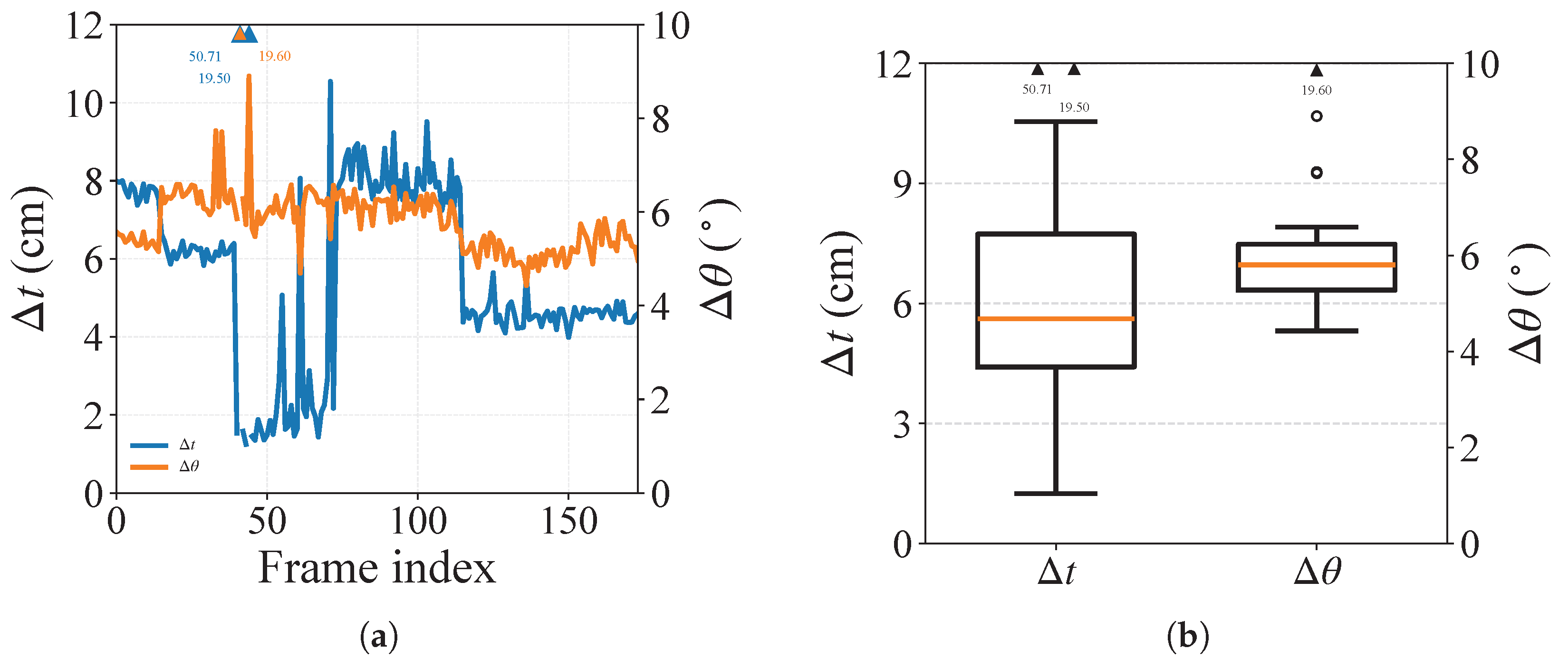
References
- Rémouit, F.; Ruiz-Minguela, P.; Engström, J. Review of Electrical Connectors for Underwater Applications. IEEE J. Ocean. Eng. 2018, 43, 1037–1047. [Google Scholar] [CrossRef] [Scilit]
- Zhao, L.; Wu, G.; Yan, Z.; Wang, D.; Hang, D. Current Status and Trends of Wet-Mate Connectors. Intell. Mar. Technol. Syst. 2025, 3, 4. [Google Scholar] [CrossRef] [Scilit]
- Teeneti, C.R.; Truscott, T.T.; Beal, D.N.; Pantic, Z. Review of Wireless Charging Systems for Autonomous Underwater Vehicles. IEEE J. Ocean. Eng. 2021, 46, 68–87. [Google Scholar] [CrossRef] [Scilit]
- Petillot, Y.R.; Antonelli, G.; Casalino, G.; Ferreira, F. Underwater robots: From remotely operated vehicles to intervention-autonomous underwater vehicles. IEEE Robot. Autom. Mag. 2019, 26, 94–101. [Google Scholar] [CrossRef] [Scilit]
- Sivčev, S.; Coleman, J.; Omerdić, E.; Dooly, G.; Toal, D. Underwater manipulators: A review. Ocean Eng. 2018, 163, 431–450. [Google Scholar] [CrossRef] [Scilit]
- Marani, G.; Choi, S.K.; Yuh, J. Underwater Autonomous Manipulation for Intervention Missions AUVs. Ocean Eng. 2009, 36, 15–23. [Google Scholar] [CrossRef] [Scilit]
- Simetti, E.; Casalino, G.; Wanderlingh, F.; Aicardi, M. Task Priority Control of Underwater Intervention Systems: Theory and Applications. Ocean Eng. 2018, 164, 40–54. [Google Scholar] [CrossRef] [Scilit]
- Sivčev, S.; Rossi, M.; Coleman, J.; Dooly, G.; Omerdić, E.; Toal, D. Fully Automatic Visual Servoing Control for Work-Class Marine Intervention ROVs. Control Eng. Pract. 2018, 74, 153–167. [Google Scholar] [CrossRef] [Scilit]
- Yu, A.; Wang, Y.; Li, H.; Qiu, B. Automatic Alignment Method of Underwater Charging Platform Based on Monocular Vision Recognition. J. Mar. Sci. Eng. 2023, 11, 1140. [Google Scholar] [CrossRef] [Scilit]
- Ni, T.; Sima, C.; Zhang, W.; Wang, J.; Guo, J.; Zhang, L. Vision-Based Underwater Docking Guidance and Positioning: Enhancing Detection with YOLO-D. J. Mar. Sci. Eng. 2025, 13, 102. [Google Scholar] [CrossRef] [Scilit]
- Wang, X.; Yang, M.; Liu, H.; Tang, Y.; Xiao, P. Two-Stage Pose Estimation for AUV Visual Guidance Using PnP and Binocular Constraints. J. Mar. Sci. Eng. 2026, 14, 405. [Google Scholar] [CrossRef] [Scilit]
- Pavlakos, G.; Zhou, X.; Chan, A.; Derpanis, K.G.; Daniilidis, K. 6-dof object pose from semantic keypoints. In Proceedings of the 2017 IEEE International Conference on Robotics and Automation (ICRA); IEEE: New York, NY, USA, 2017; pp. 2011–2018. [Google Scholar]
- Rad, M.; Lepetit, V. Bb8: A scalable, accurate, robust to partial occlusion method for predicting the 3d poses of challenging objects without using depth. In Proceedings of the IEEE International Conference on Computer Vision (ICCV); IEEE: New York, NY, USA, 2017; pp. 3828–3836. [Google Scholar]
- Tekin, B.; Sinha, S.N.; Fua, P. Real-time seamless single shot 6d object pose prediction. In Proceedings of the IEEE Conference on Computer Vision and Pattern Recognition (CVPR); IEEE: New York, NY, USA, 2018; pp. 292–301. [Google Scholar]
- Hu, Y.; Hugonot, J.; Fua, P.; Salzmann, M. Segmentation-driven 6d object pose estimation. In Proceedings of the IEEE/CVF Conference on Computer Vision and Pattern Recognition (CVPR); IEEE: New York, NY, USA, 2019; pp. 3385–3394. [Google Scholar]
- Xiang, Y.; Schmidt, T.; Narayanan, V.; Fox, D. Posecnn: A convolutional neural network for 6d object pose estimation in cluttered scenes. arXiv 2017, arXiv:1711.00199. [Google Scholar]
- Li, Z.; Wang, G.; Ji, X. Cdpn: Coordinates-based disentangled pose network for real-time rgb-based 6-dof object pose estimation. In Proceedings of the IEEE/CVF International Conference on Computer Vision (ICCV); IEEE: New York, NY, USA, 2019; pp. 7678–7687. [Google Scholar]
- Wang, G.; Manhardt, F.; Tombari, F.; Ji, X. Gdr-net: Geometry-guided direct regression network for monocular 6d object pose estimation. In Proceedings of the IEEE/CVF Conference on Computer Vision and Pattern Recognition (CVPR); IEEE: New York, NY, USA, 2021; pp. 16611–16621. [Google Scholar]
- Labbé, Y.; Carpentier, J.; Aubry, M.; Sivic, J. Cosypose: Consistent multi-view multi-object 6D pose estimation. In Proceedings of the European Conference on Computer Vision; Springer: Cham, Switzerland, 2020; pp. 574–591. [Google Scholar]
- Hinterstoisser, S.; Lepetit, V.; Ilic, S.; Holzer, S.; Bradski, G.; Konolige, K.; Navab, N. Model based training, detection and pose estimation of texture-less 3d objects in heavily cluttered scenes. In Proceedings of the Asian Conference on Computer Vision; Springer: Berlin/Heidelberg, Germany, 2013; pp. 548–562. [Google Scholar]
- Painter, H.; Flynn, J. Current and Future Wet-Mate Connector Technology Developments for Scientific Seabed Observatory Applications. In Proceedings of the OCEANS 2006; IEEE: New York, NY, USA, 2006; pp. 1–6. [Google Scholar] [CrossRef] [Scilit]
- Fan, S.; Chang, J.; Wang, Z.; Ding, M.; Sun, H.; Zhao, Y. Research on Adaptive Cooperative Positioning Algorithm for Underwater Robots Based on Dolphin Group Cooperative Mechanism. Biomimetics 2026, 11, 82. [Google Scholar] [CrossRef] [Scilit] [PubMed]
- Joshi, B.; Modasshir, M.; Manderson, T.; Damron, H.; Xanthidis, M.; Li, A.Q.; Rekleitis, I.; Dudek, G. Deepurl: Deep pose estimation framework for underwater relative localization. In Proceedings of the 2020 IEEE/RSJ International Conference on Intelligent Robots and Systems (IROS); IEEE: New York, NY, USA, 2020; pp. 1777–1784. [Google Scholar]
- Mohammed, A.; Kvam, J.; T. Thielemann, J.; Haugholt, K.H.; Risholm, P. 6d pose estimation for subsea intervention in turbid waters. Electronics 2021, 10, 2369. [Google Scholar] [CrossRef] [Scilit]
- Sapienza, D.; Govi, E.; Aldhaheri, S.; Bertogna, M.; Roura, E.; Pairet, È.; Verucchi, M.; Ardón, P. Model-based underwater 6D pose estimation from RGB. IEEE Robot. Autom. Lett. 2023, 8, 7535–7542. [Google Scholar] [CrossRef] [Scilit]
- Zhu, J.Y.; Park, T.; Isola, P.; Efros, A.A. Unpaired image-to-image translation using cycle-consistent adversarial networks. In Proceedings of the IEEE International Conference on Computer Vision (ICCV); IEEE: New York, NY, USA, 2017; pp. 2223–2232. [Google Scholar]
- Wei, H.; Zhang, M.; Wang, C.; Wang, J.; Xie, Z.; Hu, H.; Du, P. A Novel Interpretable Intelligent Attitude Perception System for Underwater Vehicles Based on Pulsating Pressure Sensor Array. Ocean Eng. 2026, 364, 127176. [Google Scholar] [CrossRef] [Scilit]
- Denninger, M.; Sundermeyer, M.; Winkelbauer, D.; Zidan, Y.; Olefir, D.; Elbadrawy, M.; Lodhi, A.; Katam, H. BlenderProc. arXiv 2019, arXiv:1911.01911. [Google Scholar]
- McGlamery, B.L. A Computer Model for Underwater Camera Systems. In Proceedings of the Ocean Optics VI; SPIE: Bellingham, WA, USA, 1980; Volume 208, pp. 221–231. [Google Scholar]
- Jaffe, J.S. Computer Modeling and the Design of Optimal Underwater Imaging Systems. IEEE J. Ocean. Eng. 1990, 15, 101–111. [Google Scholar] [CrossRef] [Scilit]
- Yu, C.; Xiao, B.; Gao, C.; Yuan, L.; Zhang, L.; Sang, N.; Wang, J. Lite-hrnet: A lightweight high-resolution network. In Proceedings of the IEEE/CVF Conference on Computer Vision and Pattern Recognition (CVPR); IEEE: New York, NY, USA, 2021; pp. 10440–10450. [Google Scholar]
- Jordt-Sedlazeck, A.; Koch, R. Refractive Structure-from-Motion on Underwater Images. In Proceedings of the IEEE International Conference on Computer Vision (ICCV); IEEE: New York, NY, USA, 2013; pp. 57–64. [Google Scholar]
- Pedersen, M.; Bengtson, S.H.; Gade, R.; Madsen, N.; Moeslund, T.B. Camera Calibration for Underwater 3D Reconstruction Based on Ray Tracing Using Snell’s Law. In Proceedings of the IEEE Conference on Computer Vision and Pattern Recognition (CVPR) Workshops; IEEE: New York, NY, USA, 2018; pp. 1410–1417. [Google Scholar]
- Seegräber, F.; She, M.; Woelk, F.; Köser, K. A Calibration Tool for Refractive Underwater Vision. In Proceedings of the IEEE/CVF International Conference on Computer Vision (ICCV) Workshops; IEEE: New York, NY, USA, 2025; pp. 2087–2095. [Google Scholar]
- Zhang, Z. A Flexible New Technique for Camera Calibration. IEEE Trans. Pattern Anal. Mach. Intell. 2000, 22, 1330–1334. [Google Scholar] [CrossRef] [Scilit]
- Hodan, T.; Sundermeyer, M.; Labbe, Y.; Nguyen, V.N.; Wang, G.; Brachmann, E.; Drost, B.; Lepetit, V.; Rother, C.; Matas, J. Bop challenge 2023 on detection segmentation and pose estimation of seen and unseen rigid objects. In Proceedings of the IEEE/CVF Conference on Computer Vision and Pattern Recognition (CVPR); IEEE: New York, NY, USA, 2024; pp. 5610–5619. [Google Scholar]
- Peng, S.; Liu, Y.; Huang, Q.; Zhou, X.; Bao, H. Pvnet: Pixel-wise voting network for 6dof pose estimation. In Proceedings of the IEEE/CVF Conference on Computer Vision and Pattern Recognition (CVPR); IEEE: New York, NY, USA, 2019; pp. 4561–4570. [Google Scholar]
- Liu, Y.; Wen, Y.; Peng, S.; Lin, C.; Long, X.; Komura, T.; Wang, W. Gen6d: Generalizable model-free 6-dof object pose estimation from rgb images. In Proceedings of the European Conference on Computer Vision; Springer: Cham, Switzerland, 2022; pp. 298–315. [Google Scholar]
- Bukschat, Y.; Vetter, M. EfficientPose: An efficient, accurate and scalable end-to-end 6D multi object pose estimation approach. arXiv 2020, arXiv:2011.04307. [Google Scholar]
- Viviers, C.G.; Filatova, L.; Termeer, M.; de With, P.H.; van der Sommen, F. Advancing 6-DoF instrument pose estimation in variable X-ray imaging geometries. IEEE Trans. Image Process. 2024, 33, 2462–2476. [Google Scholar] [CrossRef] [Scilit] [PubMed]
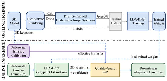
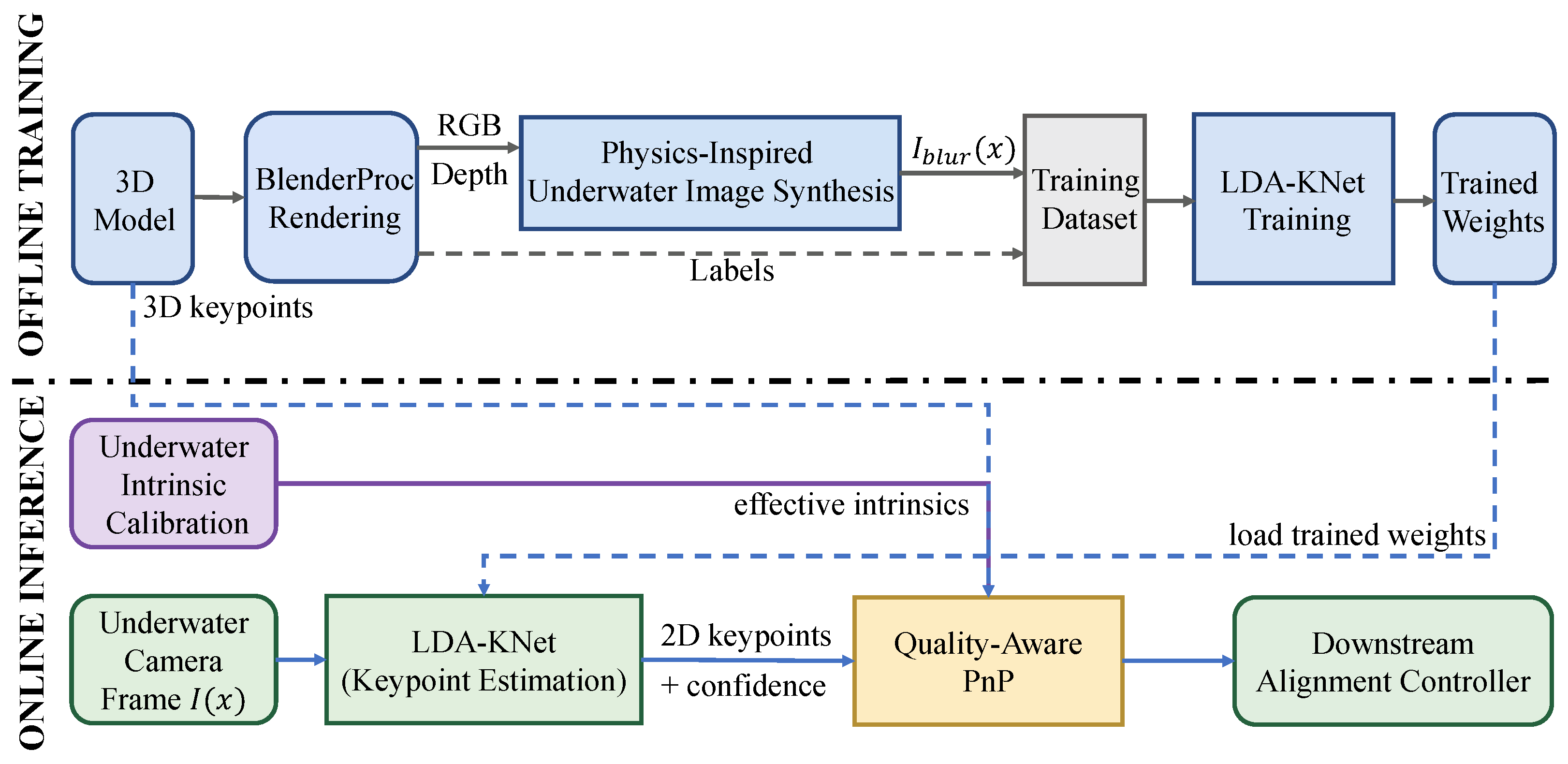
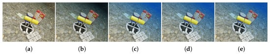
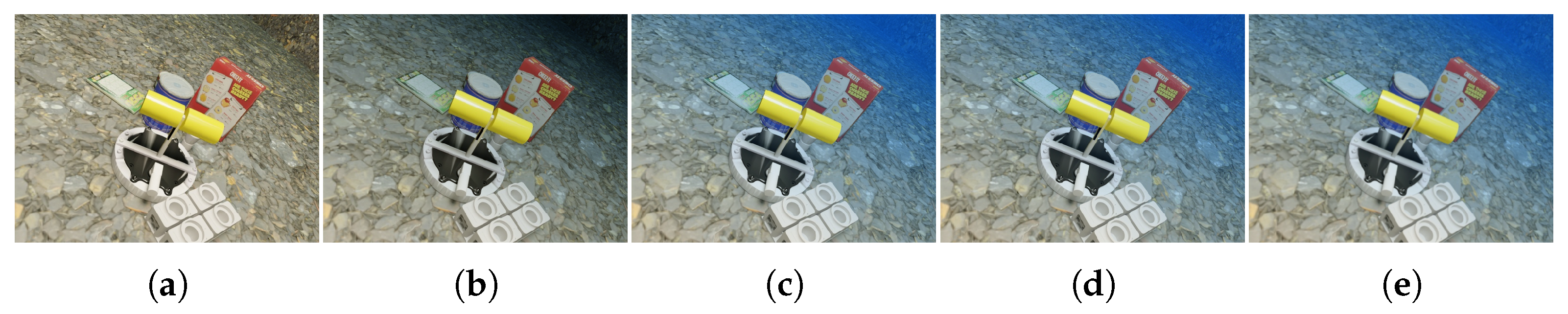
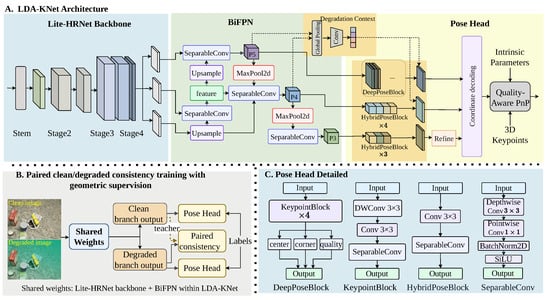
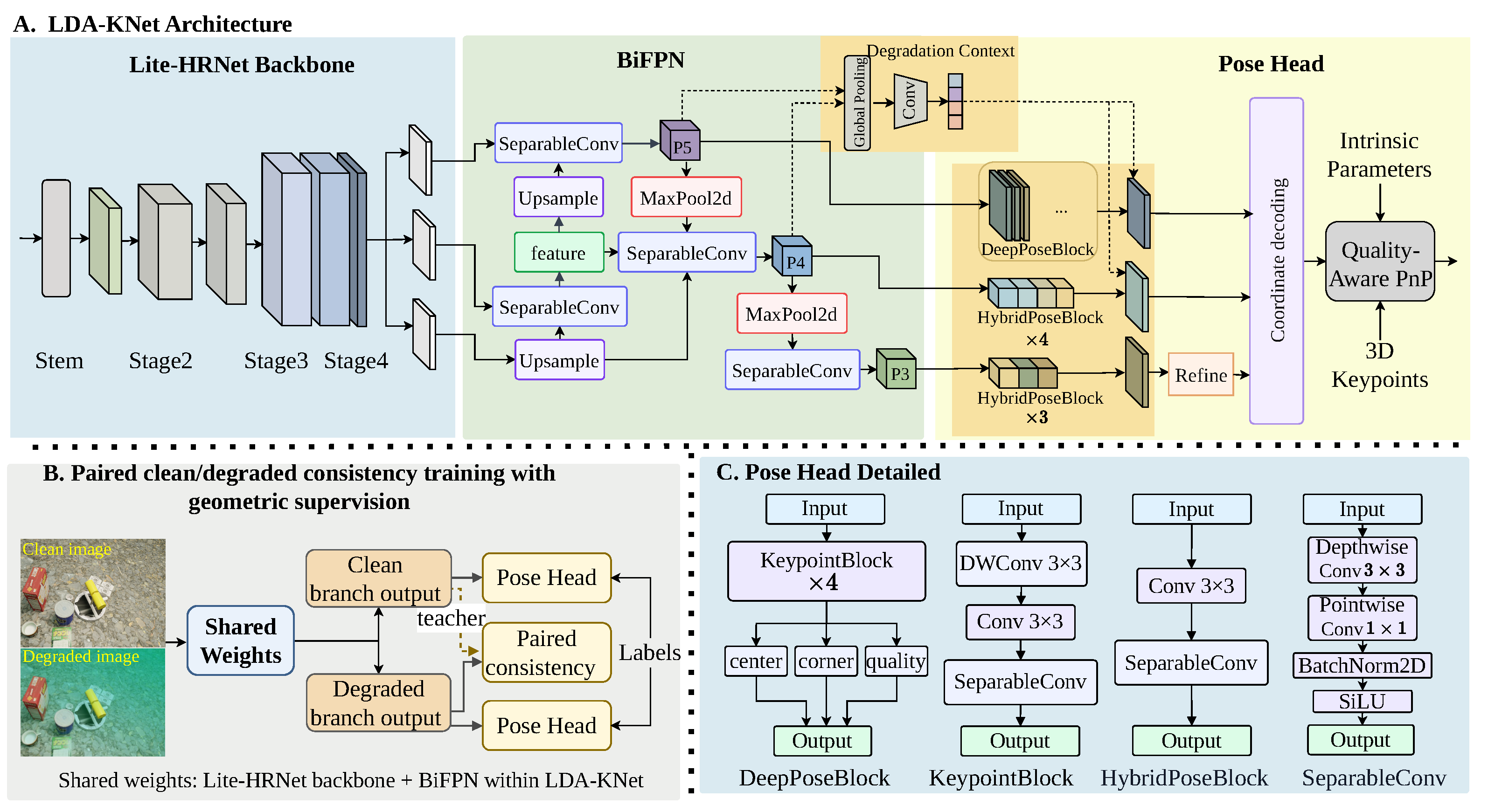
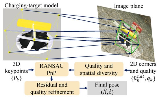
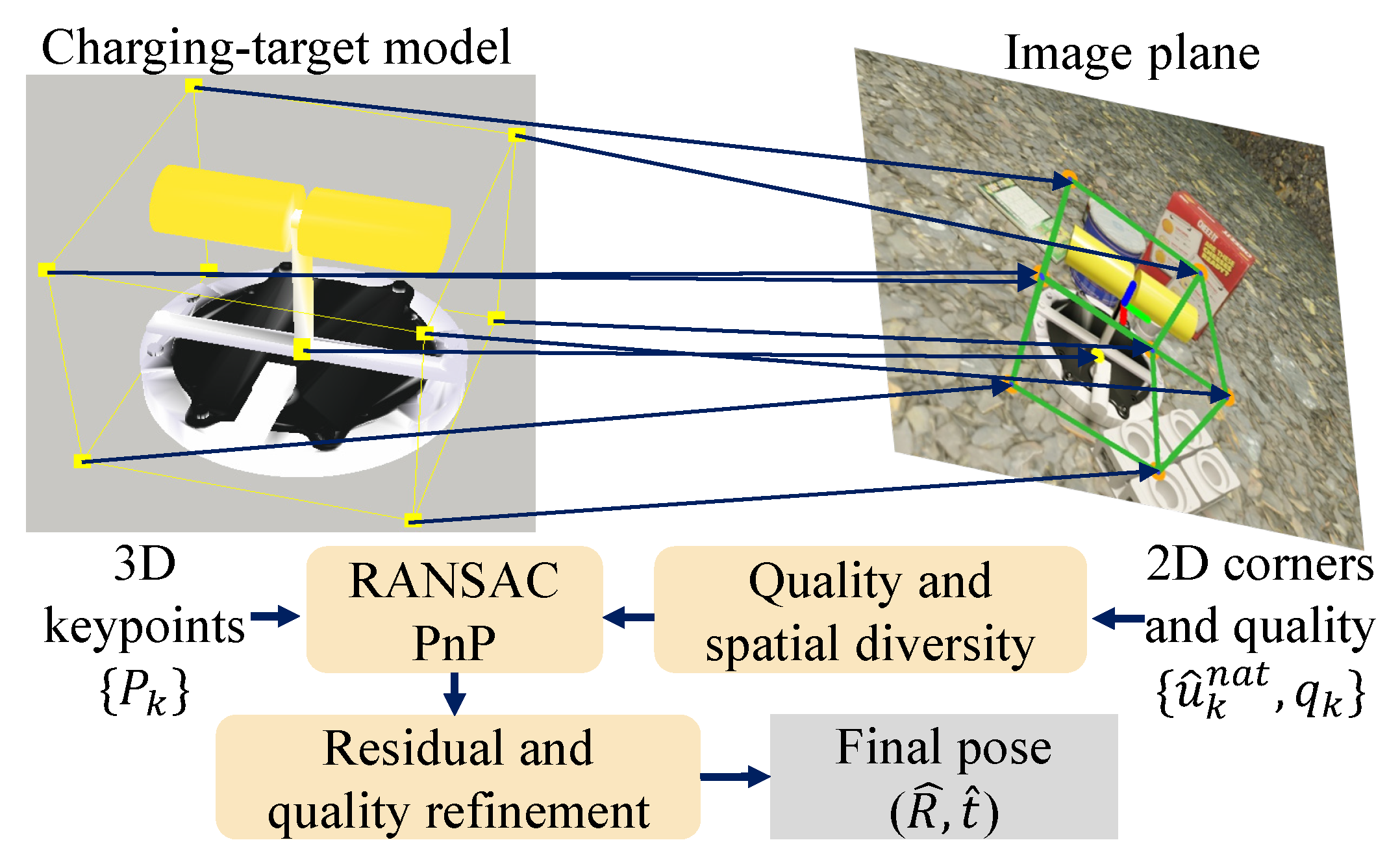
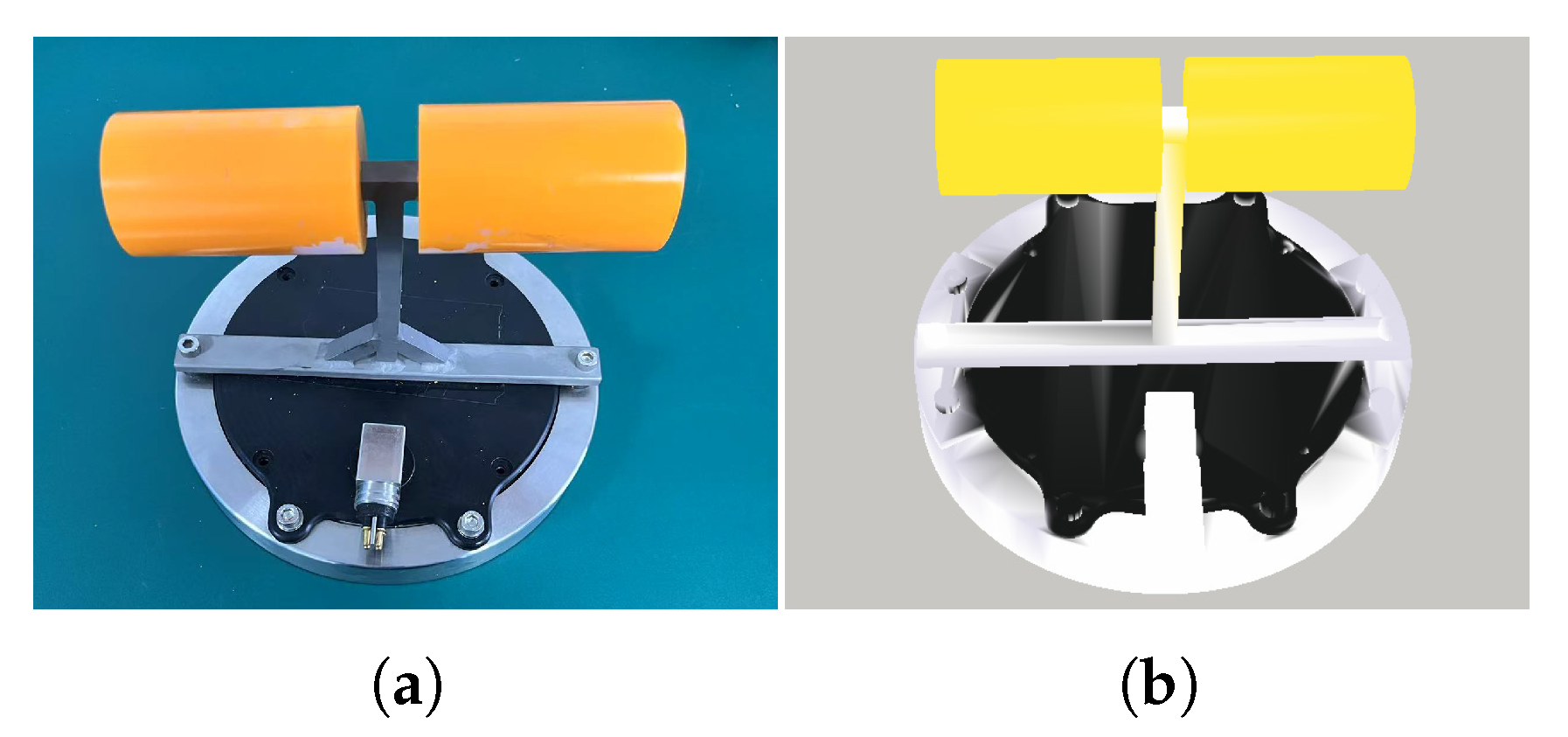
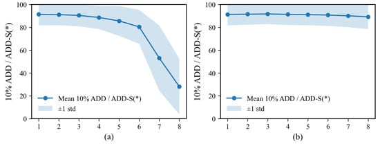
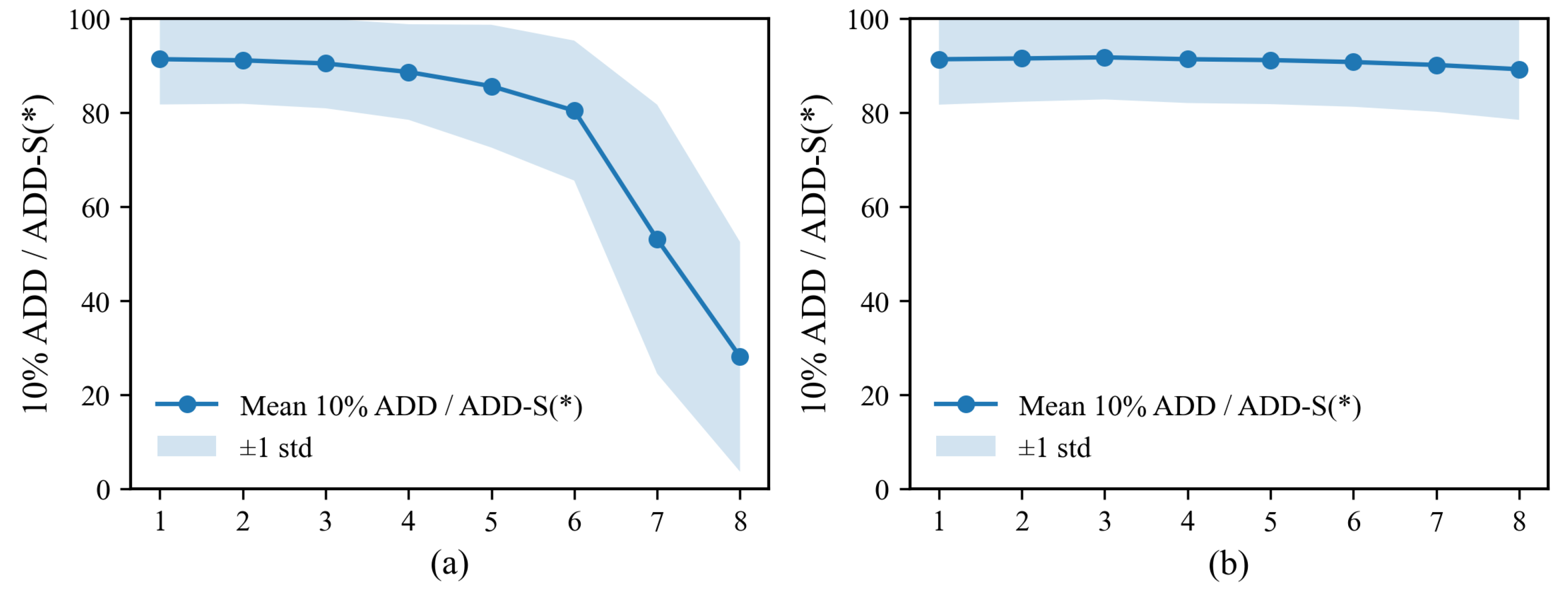
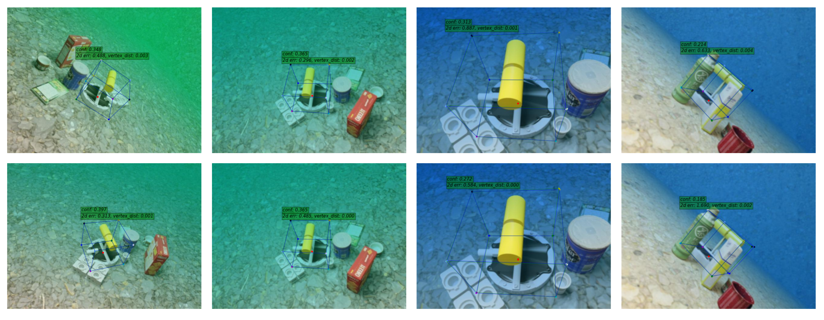
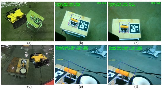
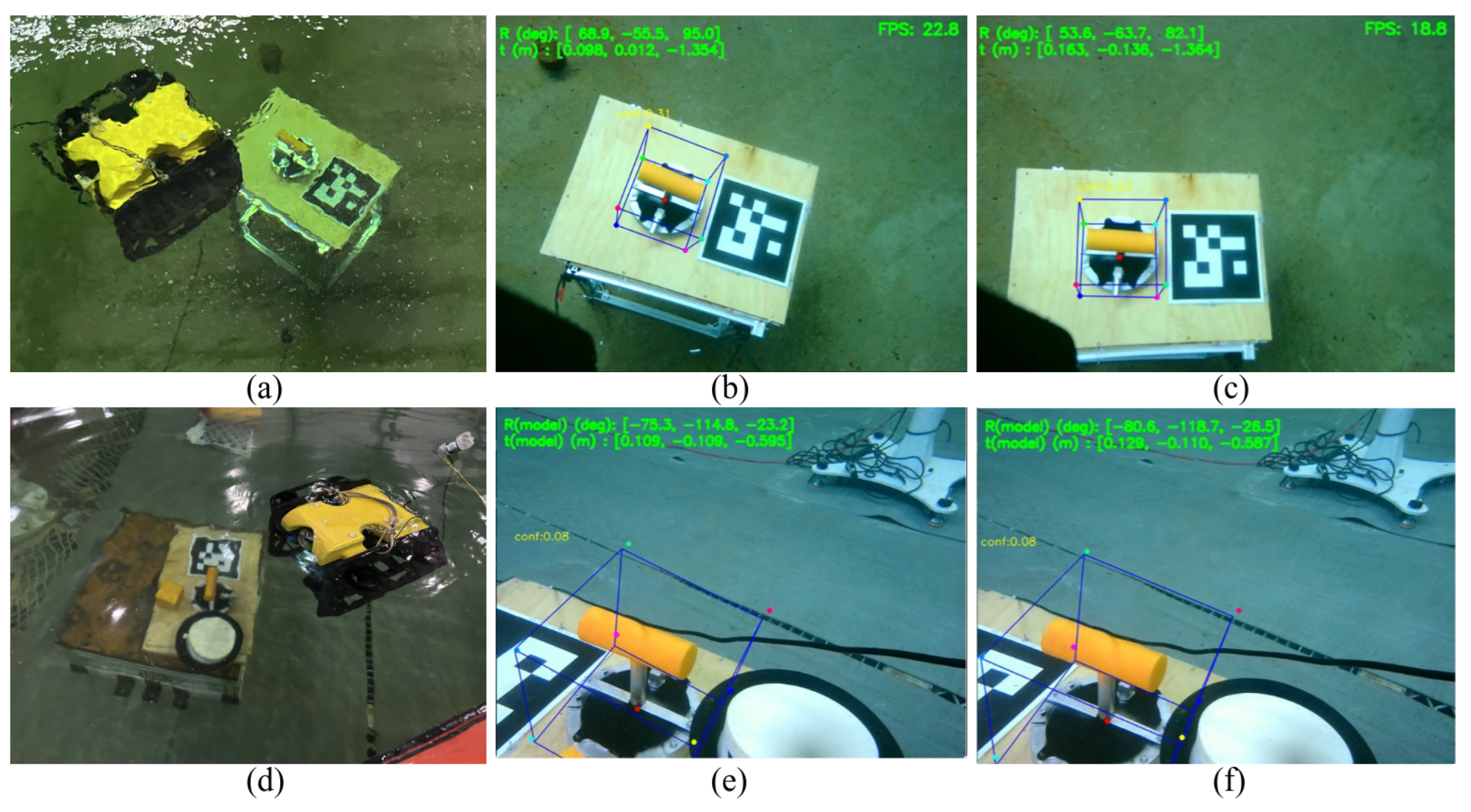
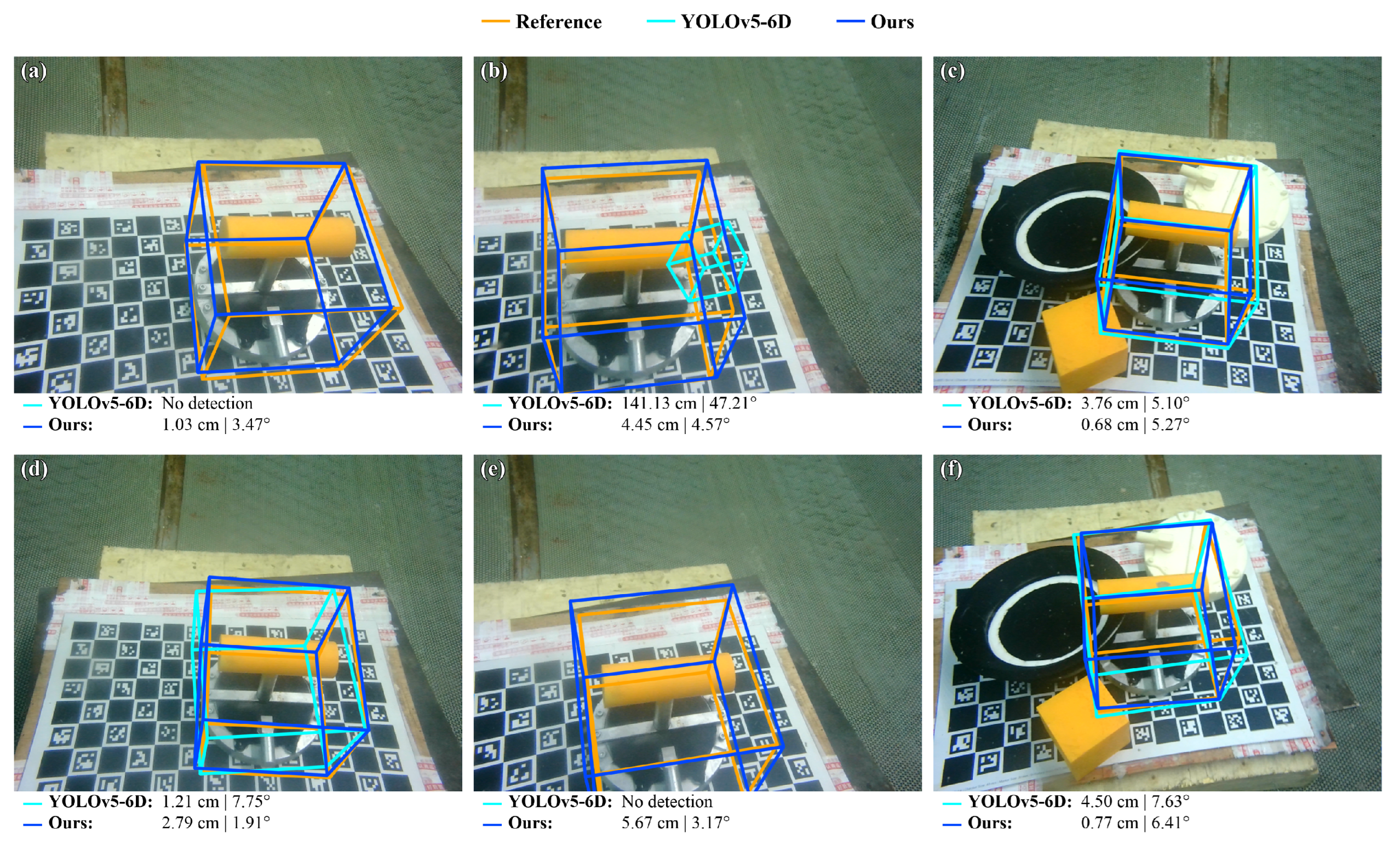

Disclaimer/Publisher’s Note: The statements, opinions and data contained in all publications are solely those of the individual author(s) and contributor(s) and not of MDPI and/or the editor(s). MDPI and/or the editor(s) disclaim responsibility for any injury to people or property resulting from any ideas, methods, instructions or products referred to in the content. |
© 2026 by the authors. Licensee MDPI, Basel, Switzerland. This article is an open access article distributed under the terms and conditions of the Creative Commons Attribution (CC BY) license.