Missingness-Aware Heterogeneous Ensemble Learning for Compression Index Prediction Across Predefined Incomplete-Input Scenarios and Unseen Marine-Clay Sites

Abstract

Reliable estimation of the compression index (Cc) is essential for settlement assessment, yet geotechnical databases often contain incomplete soil-index measurements. This study developed a missingness-aware heterogeneous ensemble that combined masked variables with binary availability indicators to predict Cc across eight predefined incomplete-input scenarios. The database comprised 1524 marine-clay specimens from eight coastal sites in South Korea. Five sites were used for model development and internal testing, while three sites were reserved for independent testing. A 12-dimensional representation allowed five artificial neural network seed models and four tree-based learners to process all scenarios using validation-derived weights. The proposed model achieved mean root mean square errors of 0.166 and 0.177 in the internal and independent tests, with corresponding coefficients of determination of 0.772 and 0.723. In the internal test, the proposed model produced more favorable point-estimate metric values than the case-specific artificial neural network and random forest baselines in all 32 comparisons and than XGBoost in 30 comparisons. The corresponding differences were less consistent in the independent test, and only six of the 24 unadjusted bootstrap confidence intervals remained entirely below zero. The framework provides a unified tool for preliminary Cc screening under the predefined incomplete-input scenarios evaluated in this study.

1. Introduction

Accurate prediction of consolidation settlement is essential for the design and maintenance of infrastructure constructed on soft ground. Excessive settlement can reduce serviceability and cause long-term performance problems in coastal facilities, reclaimed lands, and port structures [1]. The engineering behavior of structured marine clays is further complicated by installation-induced disturbance, reconsolidation, and cyclic degradation, which can substantially affect the long-term settlement and bearing performance of offshore pile foundations [2]. In conventional geotechnical design, primary consolidation settlement is commonly estimated using one-dimensional consolidation theory, in which the compression index (Cc) is one of the key parameters governing the magnitude of primary consolidation settlement [3]. However, Cc is generally obtained from oedometer consolidation tests that require high-quality undisturbed specimens and considerable testing time [4,5,6]. Therefore, empirical correlations and data-driven models are frequently used to estimate Cc from simpler index properties during preliminary design and regional ground assessment.

Empirical correlations have long been used to estimate Cc from natural water content (w_n), liquid limit (LL), plasticity index (PI), initial void ratio (e_o), and their combinations. Representative equations have been proposed using single- and multi-parameter regression forms based on w_n, LL, e_o, and related index properties [7,8,9,10,11,12,13,14,15]. For Korean coastal deposits, Yoon et al. [16] developed empirical Cc correlations using more than 1200 consolidation-test results for marine clays, providing an important regional basis for evaluating equations derived from water content, void ratio, liquid limit, and related index properties. These equations are attractive in practice because they are simple and interpretable. Nevertheless, their prediction accuracy can vary substantially when they are applied to soils from depositional environments different from those used in their derivation.

Recent studies have applied machine-learning (ML) techniques to improve Cc prediction. Neural-network-based models, including artificial neural networks (ANNs), deep neural networks, extreme learning machines, and hybrid neural models, have been used to capture nonlinear relationships between soil index properties and Cc [4,17,18,19,20,21,22]. Tree-based and ensemble-learning models, such as random forests (RFs), gradient boosting, XGBoost, stacking, and super-learner frameworks, have also been introduced to enhance prediction accuracy and robustness [23,24,25,26,27,28]. Recent civil-engineering applications have further combined multiple machine-learning models with cross-validation, interpretable feature analysis, and optimization to predict material performance and support engineering design decisions [29]. Related geotechnical applications have demonstrated optimized, interpretable, and explicit data-driven approaches across different prediction problems. Nguyen et al. [30] integrated an optimization algorithm with XGBoost to predict the seismic racking response of rectangular tunnels, while Won et al. [31] developed explicit GEP-based equations for soil-nail bond strength. Won et al. [32] further compared multiple machine-learning algorithms and used SHAP to interpret slope-stability predictions. Together, these studies demonstrate the broader potential of data-driven methods in civil and geotechnical engineering, although their performance remains strongly influenced by database composition, regional variability, and input-variable availability.

One practical limitation of existing Cc prediction models is that many of them assume a complete set of input parameters. In actual site investigations, however, a consistent suite of laboratory tests is not always performed for every specimen. Missing values may occur because of limited sampling, incomplete testing programs, or project-specific testing priorities. Incomplete records may be discarded, imputed, or processed using methods that explicitly represent missingness. Complete-case deletion can reduce the available sample size and introduce bias, whereas imputation introduces additional assumptions and uncertainty when the missingness mechanism is not adequately represented [33]. Therefore, a framework that retains the available measurements while explicitly identifying unavailable inputs is valuable under realistic geotechnical investigation conditions.

Another important limitation is the evaluation of spatial generalization. Many previous models were trained and tested using random splits from a single compiled database [4,17,21,22,28]. For spatially structured data, specimen-level random splitting can yield optimistic performance estimates because observations from the same site or region are not fully independent across the training and test sets [34]. In engineering practice, prediction models are often applied to project sites that were not included during model development. Therefore, independent-site evaluation is necessary to determine whether a model can be transferred to unseen coastal deposits.

Recent Cc studies have moved from conventional regression toward broader machine-learning frameworks, including global super learners, explainable ensemble models, variable-combination screening, and feature-missingness approaches incorporating geographical information [26,27,28,35,36]. Hamdaoui et al. [37] recently combined gradient-boosting models, hyperparameter optimization, cross-validation, and SHAP analysis to develop an interpretable Cc-prediction framework for clays. Among studies addressing unavailable inputs and geographical variability, Pang et al. [36] incorporated latitude, longitude, and climatic variables directly as predictive inputs and used a mutual prediction procedure to reconstruct unavailable soil properties before routing the reconstructed inputs to trunk and branch models. Together, these advances indicate that prediction accuracy depends not only on the model type, but also on input availability, the treatment of unavailable variables, and regional variability. Nevertheless, the combined use of explicit availability encoding, shared learning across predefined input configurations, and location-based independent testing remains insufficiently examined.

To address this gap, this study proposes a missingness-aware prediction framework for estimating Cc of Korean marine clay deposits. A database of 1524 soil specimens was compiled from eight coastal geotechnical investigation sites. Eight predefined missing-input scenarios, denoted C1–C8, were constructed to represent practical cases in which selected soil parameters were unavailable. Unlike Pang et al. [36], the proposed framework does not use geographical variables as predictive inputs or reconstruct unavailable soil properties. Location information is used exclusively for data partitioning and independent-site evaluation, whereas unavailable inputs are represented through zero masking and binary availability indicators. The scaled soil parameters and availability indicators are then processed within a shared heterogeneous ensemble, enabling the model to learn the available values and their corresponding input-availability patterns simultaneously.

The objectives of this study are to (1) compile and harmonize a multi-site database for Cc prediction, (2) construct predefined missing-input scenarios representing selected practical input-availability conditions, (3) develop a missingness-aware heterogeneous ensemble that can use incomplete input combinations, and (4) compare the proposed model with empirical correlations and case-specific machine-learning baselines. The main contribution of this study is the integration of explicit missingness encoding, validation-derived global blending, location-based independent testing, and empirical and data-driven benchmark comparisons within a unified Cc-prediction framework.

2. Database Development and Preprocessing

2.1. Study Sites and Laboratory Testing Standards

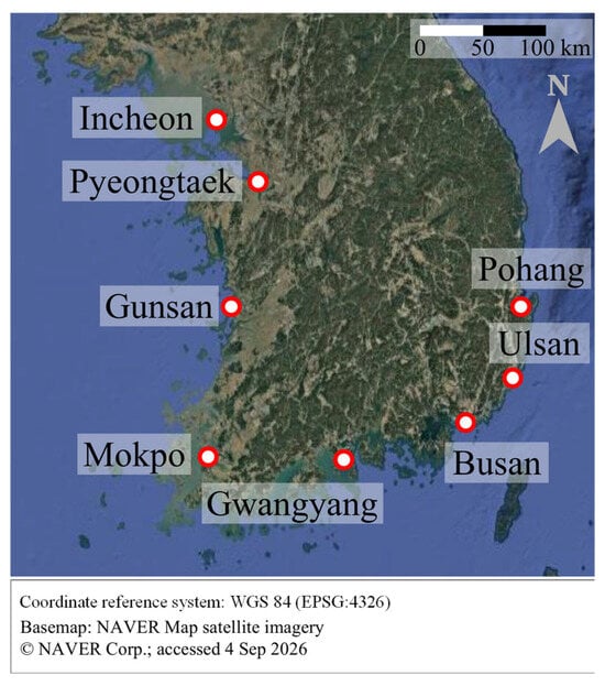
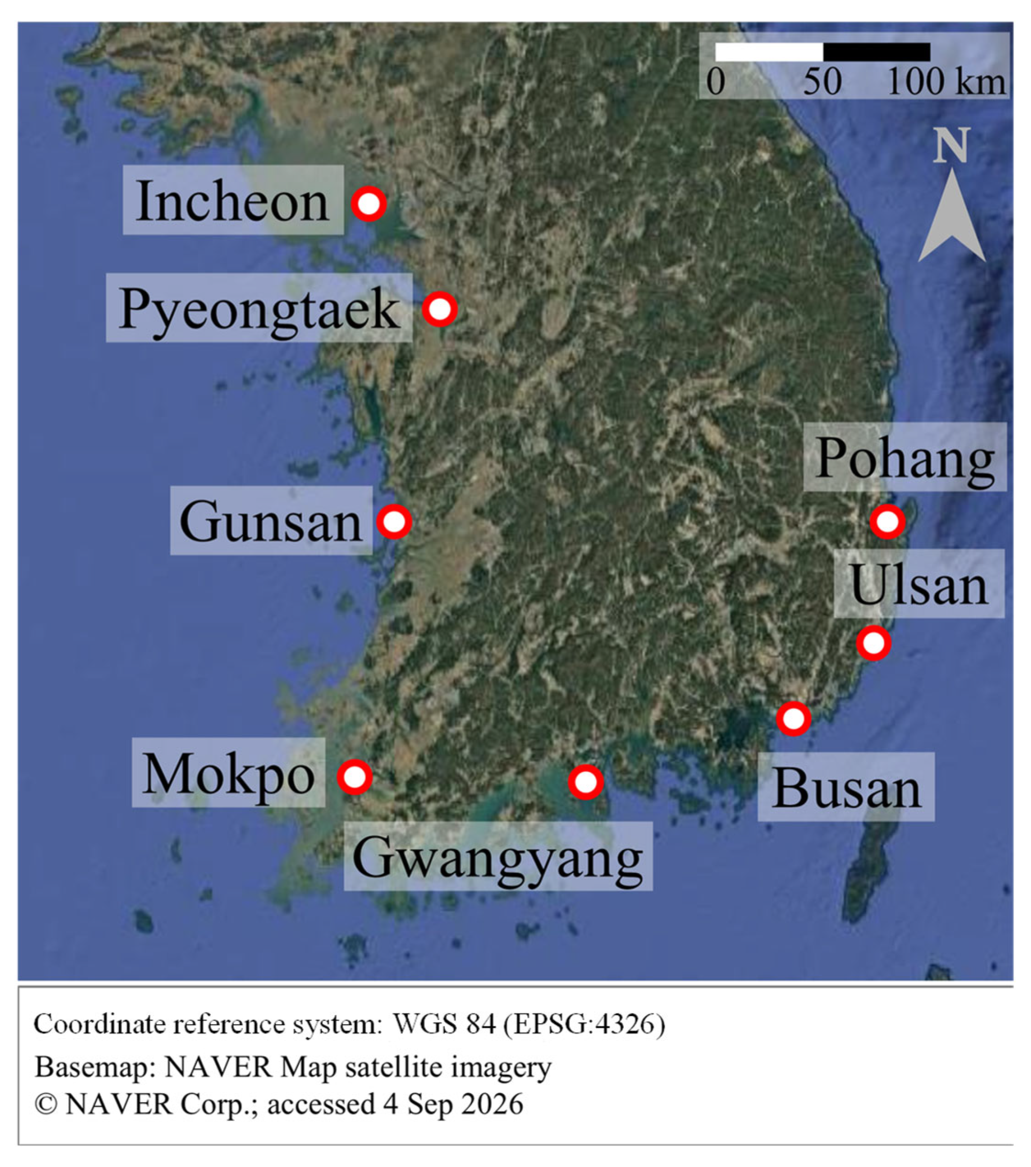
As shown in Figure 1, the geotechnical database used in this study was compiled from field investigations conducted at eight coastal development sites in South Korea. The sites were associated with port infrastructure, harbor construction, reclamation, and soft-ground improvement projects. Because they are distributed along the western, southern, and eastern coastal regions of the Korean Peninsula, the database includes marine clay deposits formed under different regional and depositional conditions.

Figure 1. Locations of the eight coastal marine-clay study sites in South Korea.

The western coastal sites, including Pyeongtaek, Incheon, Mokpo, and Gunsan, are generally associated with Holocene estuarine or tidal-flat deposits formed under macrotidal conditions [38,39,40]. The eastern and southeastern sites of Pohang and Ulsan are associated with marine deposits influenced by terrigenous sediment supply, postglacial sea-level change, and local sediment reworking and redeposition [41,42]. The Busan deposits are located predominantly within the Nakdong River delta and include tidal-flat, inner-shelf, and shallow-marine depositional units [43]. The Gwangyang deposits comprise highly compressible marine sediments whose characteristics have also been influenced by extensive dredging and reclamation activities [39,44]. These descriptions provide regional geological and depositional context rather than borehole-specific stratigraphic interpretations.

High-quality undisturbed samples were retrieved from marine clay layers using thin-walled tube samplers, and laboratory tests were performed to characterize their physical, index, and compressibility properties. Table 1 summarizes the number of specimens, investigation year(s), number of boreholes, and sampling depth for each study site. Exact specimen-specific sampling dates were not retained in the compiled database; therefore, the investigation year(s) represent project-level periods determined from the corresponding geotechnical investigation projects and source records. The database contains 1524 specimens collected from 680 identifiable boreholes during projects conducted between 1995 and 2024.

Table 1. Summary of specimens, investigation periods, boreholes, and sampling depths.

Site	Number of Specimens	Investigation Year(s)	Number of Boreholes	Sampling Depth (Mean)
Pohang	22	2011	6	7.8–21.8 m (13.82 m)
Ulsan	92	2008–2016	39	2.0–27.0 m (10.62 m)
Pyeongtaek	101	2005–2014	42	0.9–16.4 m (6.19 m)
Mokpo	101	2008–2022	35	0.8–20.3 m (6.97 m)
Gunsan	107	2004–2015	80	1.0–22.8 m (8.28 m)
Incheon	191	2001–2020	104	0.0–22.8 m (6.37 m)
Busan	356	1995–2023	126	0.9–56.4 m (15.56 m)
Gwangyang	554	1997–2024	248	1.0–30.0 m (8.39 m)
Total	1524	1995–2024	680	0.0–56.4 m (9.94 m)

The sampling depths ranged from 0.0 to 56.4 m, with an overall mean of 9.94 m. When a sampling depth was reported as an interval, the midpoint of that interval was used to calculate the site-level mean sampling depth. Differences in spacing and hyphenation within borehole identifiers were standardized before the number of boreholes was determined.

The laboratory testing program followed standardized test methods. Natural water content (w_n) was determined by oven drying in accordance with ASTM D2216-19 [45]. The liquid limit (LL) and plasticity index (PI) were obtained from Atterberg limit tests following ASTM D4318-17e1 [46]. The clay-size fraction (CF), defined as the percentage by mass of particles finer than 2 μm, was determined by sedimentation analysis in accordance with ASTM D7928-21e1 [47]. The initial void ratio (e_o) was obtained from the source investigation records or determined from the initial specimen condition using the available mass–volume and physical-property information. When the water content, specific gravity, and degree of saturation were available, e_o could be calculated from e_o = wGs/Sr, where w is the water-content ratio, Gs is the specific gravity, and Sr is the degree of saturation. For a saturated specimen with w_n expressed as a percentage, this relationship reduces to e_o ≈ (w_n/100)Gs. Accordingly, determination of e_o does not necessarily require completion of the incremental-loading consolidation test. Soil activity (Act.) was calculated as the ratio of PI to CF following Skempton [48] and was therefore treated as a derived feature rather than an independent measurement.

According to the available project reports and source records, the one-dimensional consolidation tests were conducted in accordance with ASTM D2435/D2435M-25 [49]. Depending on the source geotechnical investigation project, one of two nominal vertical-stress schedules was used: (i) 12, 25, 50, 100, 200, 400, and 800 kPa or (ii) 5, 10, 20, 40, 80, 160, 320, 640, and 1280 kPa. In both schedules, the applied vertical stress was approximately doubled at each successive loading stage, corresponding to a load increment ratio (LIR) of approximately 1.

The Cc values used in the present database were obtained from historical site-investigation records and source datasets rather than being uniformly recalculated by the present authors from the original consolidation curves. According to the documented practices of the source investigations, preconsolidation stress was determined using the Casagrande method in most projects, the virgin-compression range was selected manually, and Cc was generally estimated as the absolute slope of a linear regression fitted to three or more loading points. Although the reported testing procedures were consistent with ASTM D2435, the original consolidation curves and specimen-level calculation records were not retained for every specimen. Consequently, compliance with every procedural detail and the uniformity of Cc interpretation across all 1524 specimens could not be retrospectively confirmed. This limitation concerns the traceability and uniformity of the historical specimen-level calculations rather than evidence that the tests were conducted using nonstandard procedures. Information required to consistently classify the specimens as normally consolidated or overconsolidated was unavailable for most records; therefore, consolidation state was not used as an input variable or specimen-selection criterion.

The selected variables were used because they are closely related to the compressibility of fine-grained soils [4,8,12,19,28,35,50]. w_n and e_o describe the initial moisture and void state of the soil, whereas LL and PI reflect plasticity and clay-mineral effects. CF describes the clay-size fraction, whereas Act. explicitly represents plasticity relative to CF. Because Act. is mathematically derived from PI and CF, it does not constitute an additional independent measurement. The variables were selected based on their established physical relevance and availability across the compiled database. In practical applications, w_n, LL, PI, CF, and e_o may be obtained from routine physical and index characterization or existing geotechnical investigation records without completing the full incremental-loading procedure required to determine Cc. The resulting physically relevant feature set therefore supports preliminary Cc screening and data-driven prediction when complete consolidation-test results are unavailable.

During database compilation, the records were checked for the availability and numerical validity of the variables required for model development. Site names, borehole identifiers, variable definitions, and measurement units were standardized across the source projects. No statistical outlier-removal procedure or additional value-based quality-control threshold was applied, because the natural variability of the multi-site marine-clay database, including relatively rare high-Cc specimens, was retained. Potential duplicate records were screened programmatically using the study site, standardized borehole identifier, sampling depth, input variables, and Cc, and were cross-checked against the original project information and source records. This examination confirmed that no duplicate records were present in the final database. To the best of the authors’ knowledge, the database was not directly obtained from or intentionally combined with specimen-level databases used in previous Korean compression index studies. Nevertheless, incidental overlap cannot be conclusively excluded because some previous studies were also based on Korean coastal geotechnical investigation projects and did not provide publicly accessible record-level identifiers.

2.2. Database Characterization

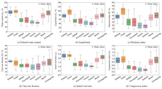
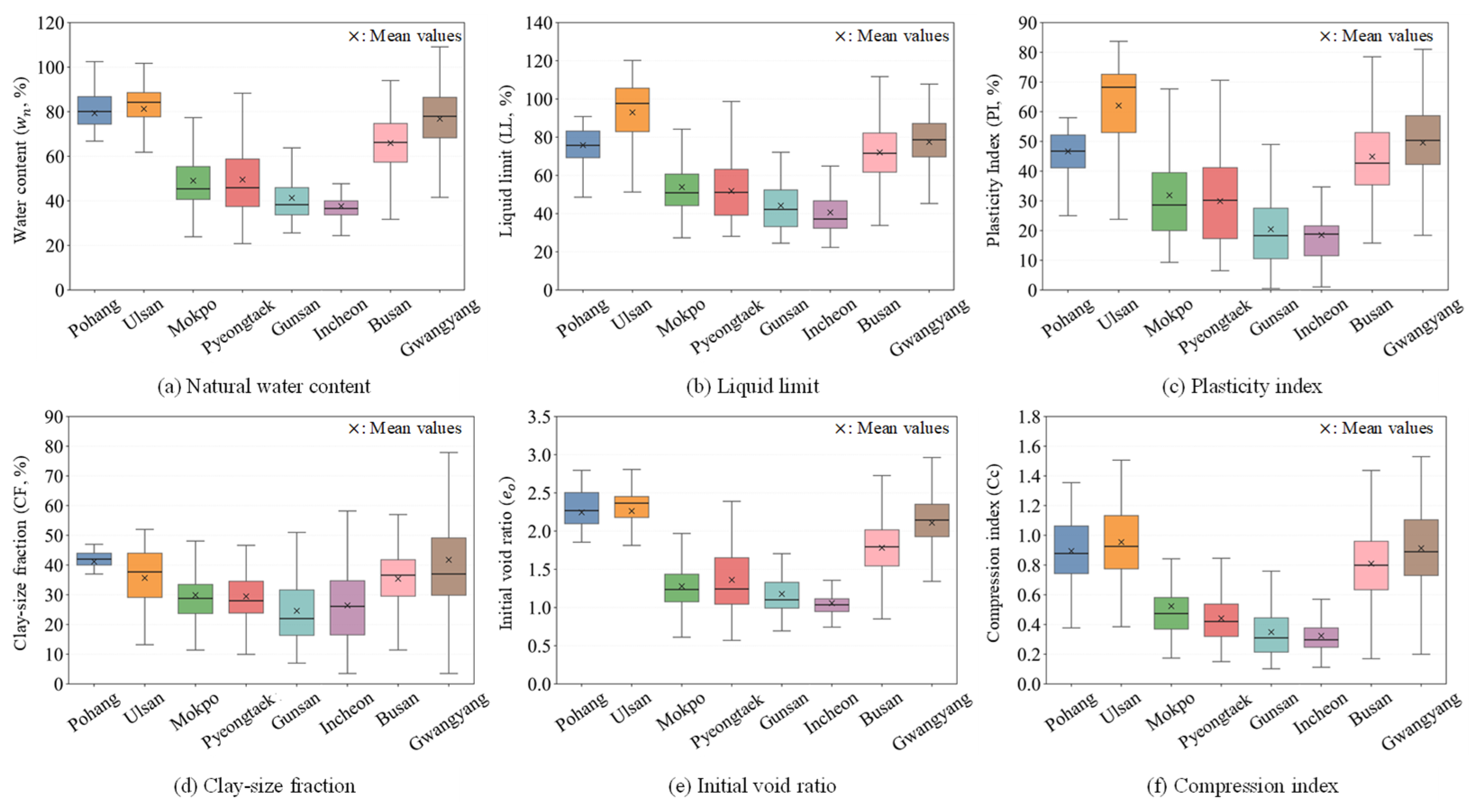
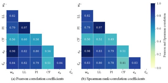
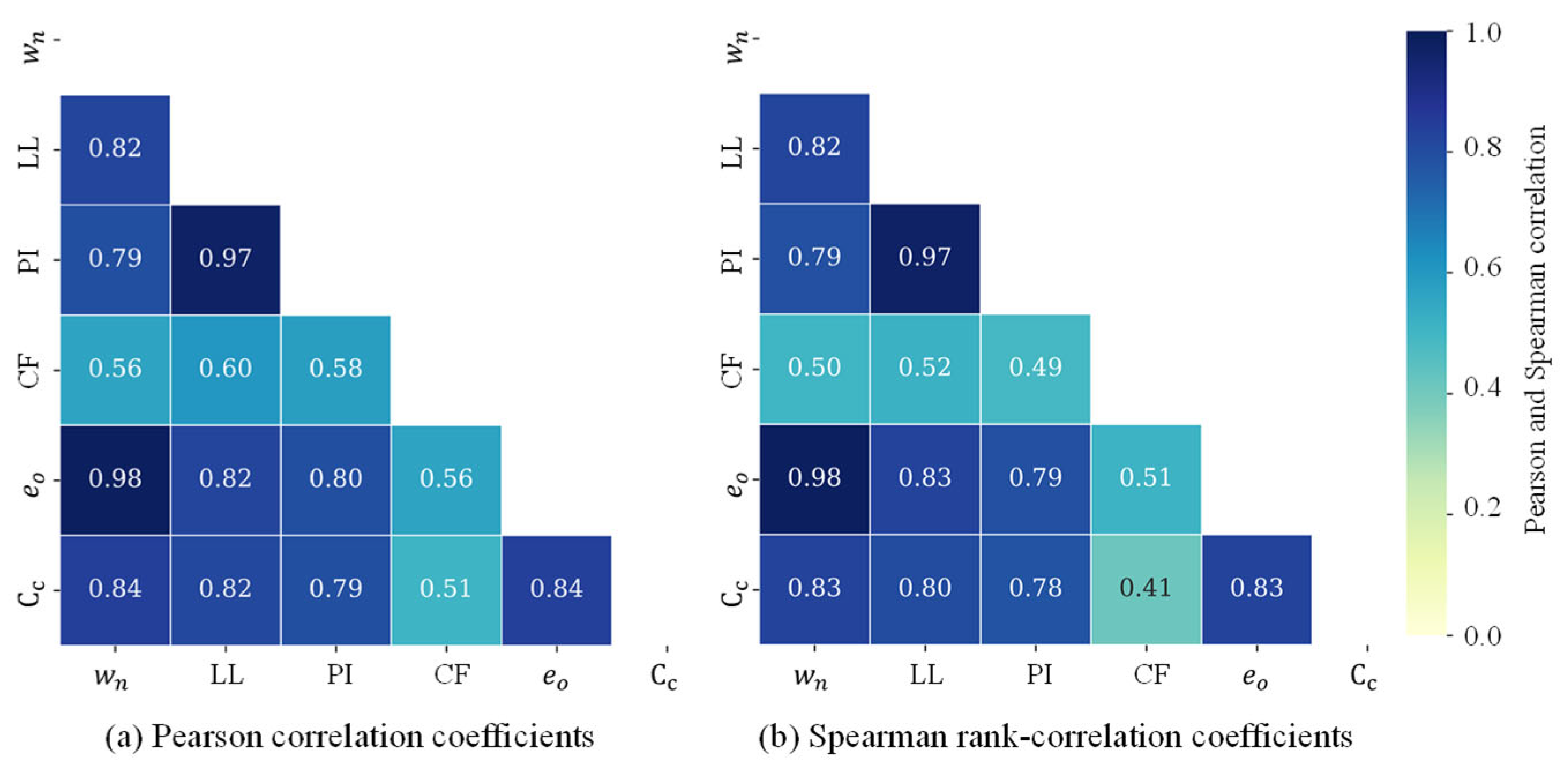
Table 2 and Figure 2 summarize the descriptive statistics and site-wise distributions of the database, respectively. Table 2 lists the mean and standard deviation for each study site, whereas Figure 2 presents the distributions of the measured soil parameters. Activity was reported in Table 2 but excluded from Figure 2 to keep the graphical comparisons focused on directly measured variables. Activity was also excluded from the correlation matrix in Figure 3 because it is mathematically determined by PI and CF rather than independently measured. Including Act. alongside PI and CF could cause correlations arising from this deterministic relationship to be interpreted as independent correlation evidence. Act. was nevertheless retained as a model input because it provides an established engineered descriptor of plasticity relative to the clay-size fraction.

Table 2. Site-wise mean and standard deviation of the soil index and compressibility properties.

Site	N	wn (%)	LL (%)	PI (%)	CF (%)	Act.	eo	Cc
Pohang	22	79.32 ± 14.19	75.84 ± 13.21	46.65 ± 10.08	41.18 ± 4.63	1.13 ± 0.18	2.25 ± 0.41	0.89 ± 0.26
Ulsan	92	81.29 ± 13.99	92.99 ± 17.70	62.06 ± 15.89	35.67 ± 9.29	1.79 ± 0.46	2.26 ± 0.36	0.95 ± 0.26
Mokpo	101	49.07 ± 12.62	53.87 ± 14.71	31.89 ± 14.38	29.90 ± 9.67	1.07 ± 0.33	1.28 ± 0.40	0.52 ± 0.23
Pyeongtaek	101	49.54 ± 15.10	66.91 ± 21.21	40.79 ± 18.60	35.17 ± 14.81	1.21 ± 0.51	1.74 ± 0.55	0.72 ± 0.34
Gunsan	107	45.08 ± 12.13	48.89 ± 14.60	26.01 ± 14.26	27.18 ± 11.24	0.97 ± 0.38	1.23 ± 0.35	0.43 ± 0.22
Incheon	191	37.63 ± 7.23	40.62 ± 11.62	18.50 ± 10.03	26.43 ± 12.08	0.71 ± 0.24	1.06 ± 0.20	0.32 ± 0.13
Busan	356	65.97 ± 11.53	72.04 ± 15.59	44.90 ± 14.59	35.39 ± 9.52	1.32 ± 0.44	1.78 ± 0.31	0.81 ± 0.25
Gwangyang	554	76.84 ± 15.47	77.50 ± 14.36	49.59 ± 13.49	41.77 ± 17.76	1.34 ± 0.51	2.11 ± 0.41	0.91 ± 0.29

Figure 2. Site-wise distributions of the soil index and compressibility properties.

Figure 3. Pearson and Spearman correlations among the soil properties and compression index (Cc).

The database showed clear regional variability in the index and compressibility properties. Incheon had the lowest mean values of w_n (37.6%), LL (40.6%), PI (18.5%), e_o (1.06), and Cc (0.32). These values represented the lowest plasticity and compressibility among the study sites. In contrast, Ulsan had the highest mean values of LL (93.0%), PI (62.1%), Act. (1.79), e_o (2.26), and Cc (0.95). These values represented the highest plasticity and compressibility among the study sites.

Pohang and Gwangyang also exhibited relatively high w_n, e_o, and Cc. These characteristics were consistent with soft and highly compressible soil conditions. Busan and Pyeongtaek showed intermediate characteristics, with average Cc values of 0.81 and 0.72, respectively. These trends indicate that the database covers a broad range of marine clay conditions suitable for model development and validation.

Figure 3 illustrates the relationships among the soil parameters and Cc. In the figure, the Pearson correlation was used to quantify linear association, whereas Spearman rank correlation was used to evaluate monotonic association based on ranked data [51,52,53]. These two measures are commonly used to identify influential variables before statistical or machine-learning-based Cc prediction models are developed [28,35].

The correlation analysis showed that w_n, LL, PI, and e_o were more strongly related to Cc. This trend is consistent with the physical roles of water content, plasticity, and void ratio in controlling compressibility [12,14,15,50]. In contrast, CF showed a weaker direct correlation with Cc. Nevertheless, CF was retained because it provides complementary information on the clay-size fraction and enables soil activity to be calculated [48].

2.3. Location-Based Data Partitioning and Missing-Input Scenario Construction

A location-based partitioning strategy was applied to assess model performance at both represented and unseen sites. Pyeongtaek, Pohang, and Ulsan were designated as independent test sites before model development. Busan and Gwangyang, which together contributed approximately 59.7% of the specimens, were retained in the model-development dataset to provide sufficient sample size and coverage of the input-property and Cc ranges. The independent sites provided complementary conditions: Pyeongtaek represented transfer to a new western coastal site, whereas Pohang and Ulsan represented eastern and southeastern coastal settings not directly included in model development. All specimens from these three sites were excluded from training, validation, and hyperparameter optimization. The remaining five sites were used to construct the training, validation, and internal test sets through a 7:1:2 allocation. The models were trained at the specimen level, with each specimen contributing equally to the training objective. Site-balanced weighting was not applied, and site identifiers were not included as model inputs.

Within each of the five model-development sites, the Cc range was divided into 10 intervals. The specimens in each interval were then randomly allocated to the training, validation, and internal test sets at proportions of 70%, 10%, and 20%, respectively. The resulting specimen assignments were fixed and applied consistently throughout all subsequent analyses, as summarized in Table 3.

Table 3. Location-based partitioning of the database.

Site	Train	Validation	Internal Test	Independent Test
Pohang	-	-	-	22
Ulsan	-	-	-	92
Pyeongtaek	-	-	-	101
Mokpo	69	10	22	0
Gunsan	73	10	24	0
Incheon	132	17	42	0
Busan	247	35	74	0
Gwangyang	382	52	120	0

Because the allocation was performed at the specimen level, physically distinct specimens collected from different depths of the same borehole could be assigned to different subsets. These specimens were treated as separate observational units because they may represent different soil layers and stress histories. Nevertheless, specimens from the same borehole may share local stratigraphic and depositional characteristics.

The internal test set therefore evaluated new specimens from locations represented during model development under the existing borehole sampling structure, rather than strict generalization to entirely unseen boreholes. In contrast, the independent test set evaluated transfer to three geographically distinct sites that were not involved in model development. This design provided a more spatially separated assessment than a conventional random specimen-level split.

Table 4 summarizes the eight input scenarios constructed to simulate practical incomplete-input conditions. C1 represents the complete-input condition; C2 excludes w_n; C3 excludes LL, PI, and Act.; C4 excludes CF and Act.; C5 excludes e_o; C6 excludes w_n and e_o; C7 excludes w_n, LL, PI, and Act.; and C8 excludes LL, PI, CF, and Act. Activity was treated as unavailable whenever PI or CF was missing because it was calculated from these two parameters.

Table 4. Input configurations for the eight incomplete-input scenarios.

Case	wn	LL	PI	CF	Act.	eo	Description
C1	✓	✓	✓	✓	✓	✓	All input variables available
C2	-	✓	✓	✓	✓	✓	Water content unavailable
C3	✓	-	-	✓	-	✓	Atterberg limits unavailable
C4	✓	✓	✓	-	-	✓	Clay-size fraction unavailable
C5	✓	✓	✓	✓	✓	-	Initial void ratio unavailable
C6	-	✓	✓	✓	✓	-	Water content and initial void ratio unavailable
C7	-	-	-	✓	-	✓	Water content and Atterberg limits unavailable
C8	✓	-	-	-	-	✓	Atterberg limits and clay-size fraction unavailable

Note: ✓ indicates an available input variable; - indicates an unavailable input variable.

These scenarios were generated by withholding predefined groups of variables from otherwise complete specimen records. They therefore represent structured incomplete-input configurations rather than naturally occurring missingness patterns. The present evaluation was not designed to distinguish among missing completely at random, missing at random, and missing not at random mechanisms. The same eight input-availability configurations were represented across the training, validation, internal-test, and independent-test sets. Accordingly, the evaluation examined predictions for unseen specimens and sites under known missingness configurations rather than generalization to previously unseen missingness patterns.

The location-based data split was kept identical across all missing-input scenarios. The training, validation, internal-test, and independent-test specimens therefore remained unchanged across C1–C8. The validation set contained 124 unique specimens and generated 992 scenario-specific rows across C1–C8. These rows represented correlated incomplete-input versions of the same specimens and were not treated as independent observations. All eight versions of each specimen remained within the same data partition.

This consistent partitioning allowed scenario-level performance differences to be attributed primarily to input availability rather than variation in the specimens used for model development and evaluation. In addition, all preprocessing parameters were estimated using only the training data. The fitted parameters were subsequently applied without refitting to the validation, internal-test, and independent-test sets, thereby preventing validation or test information from entering model development through preprocessing.

3. Methods and Model Development

3.1. Missingness-Aware Heterogeneous Ensemble Framework

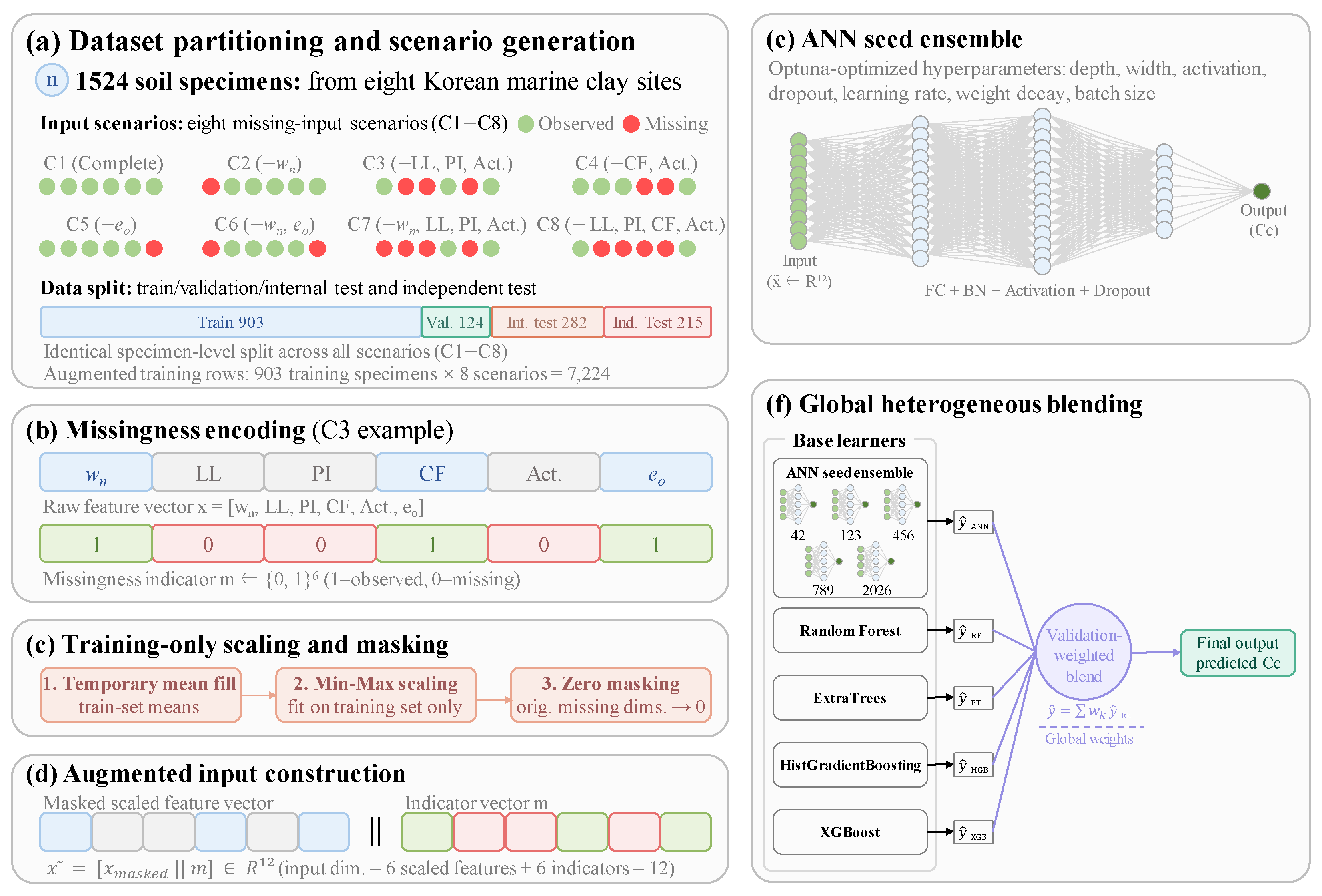
Figure 4 presents the proposed missingness-aware heterogeneous ensemble framework for Cc prediction. Here, missingness-aware refers to the explicit representation of unavailable inputs through zero masking and binary availability indicators rather than statistical inference of the missing-data mechanism. The framework comprises dataset partitioning and scenario generation, missingness encoding, training-only scaling and masking, augmented input construction, ANN seed ensembling, and validation-weighted global heterogeneous blending.

Figure 4. Workflow of the missingness-aware heterogeneous ensemble framework.

Figure 4a summarizes dataset partitioning and scenario generation. The database comprised 1524 specimens from eight marine-clay sites, and the eight predefined missing-input scenarios C1–C8 were generated according to Table 4. Five sites supplied 903 training, 124 validation, and 282 internal-test specimens, whereas the three geographically distinct sites supplied 215 independent-test specimens. The specimen-level split was kept identical across C1–C8. Accordingly, the 903 training specimens produced 7224 scenario-specific training rows. These rows represented eight correlated incomplete-input versions of the same 903 unique specimens and were not interpreted as an increase in the independent sample size. All versions of each specimen remained within the same data partition.

Figure 4b illustrates missingness encoding using C3 as an example. The raw feature vector was x = [w_n, LL, PI, CF, Act., e_o], and a corresponding indicator vector m ∈ {0, 1}⁶ identified observed and unavailable entries. In C3, LL, PI, and Act. were unavailable and assigned indicators of zero, whereas w_n, CF, and e_o were retained and assigned indicators of one.

Figure 4c shows the training-only scaling and masking sequence. Unavailable entries were temporarily filled using feature means estimated from the training data so that the six-variable array could be transformed by a min–max scaler fitted only to the training set. After scaling, entries that were originally unavailable were overwritten with zero. The temporary fill values therefore enabled numerical transformation but were never presented to the learners as observed soil properties.

Figure 4d presents augmented input construction. The masked and scaled feature vector was concatenated with the indicator vector to form $\tilde{\mathrm{x}}=[{\mathrm{x}}_{\mathrm{m}\mathrm{a}\mathrm{s}\mathrm{k}\mathrm{e}\mathrm{d}}\parallel \mathrm{m}]\in {\mathbb{R}}^{12}$. The first six elements contained the scaled soil properties with zeros at unavailable positions, and the remaining six elements described feature availability. This common representation allowed all learners to process C1–C8 while distinguishing zero-masked missing entries from observed values. The availability indicators were therefore used as deterministic descriptors of input state, and their isolated contribution to predictive performance was not evaluated in this study.

Figure 4e illustrates the ANN seed ensemble. The 12-dimensional augmented vector was processed by a fully connected ANN whose depth, width, activation function, normalization, dropout, learning rate, weight decay, loss settings, and batch size were selected through the optimization procedure described in Section 3.2. Five models were then trained using random seeds 42, 123, 456, 789, and 2026. Their predictions were combined using nonnegative validation-derived seed weights, producing one ANN seed-ensemble prediction for each specimen.

$$w_s={\left({\mathrm{r}}_{\mathrm{s}}+\epsilon \right)}^{-2}/{\displaystyle \sum _j^S}{\left(r_j+\epsilon \right)}^{-2}$$

(1)

where r_s denotes the RMSE calculated for the s-th seed model over the validation samples pooled across C1–C8, ε = 10⁻⁸ is a numerical stability constant, and S is the total number of ANN seed models (S = 5). The resulting nonnegative weights sum to one.

Figure 4f shows the global heterogeneous blending stage. The ANN seed ensemble, Random Forest [54], ExtraTrees [55], HistGradientBoosting [56], and XGBoost [57], was trained using the common 12-dimensional representation. Their predictions were combined, and a single global weight vector was selected from the validation predictions pooled across C1–C8. The same weights were subsequently applied to every scenario in the internal and independent tests, preventing test information from influencing the blend.

The same fixed validation set provided a consistent basis for hyperparameter selection, early stopping, ANN seed-weight determination, and global blending-weight optimization. The internal and independent test sets remained completely excluded from all of these model-selection procedures and were evaluated only after the model configurations and ensemble weights had been fixed.

3.2. Hyperparameter Optimization and Validation-Based Weight Determination

Hyperparameters were optimized using the tree-structured Parzen estimator sampler implemented in Optuna [58]. The ANN search comprised 5000 trials. Each trial was trained for a maximum of 500 epochs with an early stopping patience of 50 epochs. The search covered eight hidden-layer configurations, ReLU, LeakyReLU, and ELU activation functions, no normalization, batch normalization, and layer normalization. Dropout was varied from 0.0 to 0.4, the learning rate from 1.0 × 10⁻⁴ to 5.0 × 10⁻³, the weight decay from 1.0 × 10⁻⁶ to 1.0 × 10⁻³, and the batch size among 32, 64, and 128.

The Cc target was standardized using the mean and standard deviation of the expanded training target and was returned to its original scale before validation scoring. Trials were ranked using the case-balanced root mean square error, defined as the average RMSE across the eight missing-input scenarios (C1–C8), so that each scenario contributed equally to model selection. Case-balanced RMSE was also used as the primary metric for the main performance comparison. Training used a weighted Huber loss, and the Huber threshold was selected from 0.1, 0.2, 0.5, and 1.0, while each observation received the weight 1 + αCc. The coefficient α was selected from 0, 0.1, 0.25, 0.5, 0.75, and 1.0 to reduce systematic underprediction for specimens with relatively high Cc.

Table 5 summarizes the optimized hyperparameter configurations of the ANN and four tree-based learners used in the proposed framework. The selected ANN contained three hidden layers with 512, 256, and 128 neurons, LeakyReLU activation, batch normalization, and a dropout rate of 0.0003. The optimized learning rate and weight decay were 2.80 × 10⁻⁴ and 3.61 × 10⁻⁶, respectively. The selected configuration used a Huber threshold of 0.5, uniform observation weights, and a batch size of 64. The five ANN seed models were then trained for up to 1000 epochs using Adam and OneCycleLR, with early stopping after 100 epochs without sufficient validation-loss improvement.

Table 5. Optimized hyperparameters of the ANN and tree-based learners.

Model	Category	Item	Configuration
ANN	Architecture	Input dimension	12
		Hidden layers	[512, 256, 128]
		Network depth	3 hidden layers
		Activation function	LeakyReLU
		Dropout rate	0.0003
		Normalization	Batch norm.
	Optimization	Optimizer	Adam
		Learning rate	2.80 × 10−4
		Weight decay	3.61 × 10−6
		Batch size	64
		LR scheduler	OneCycleLR
	Loss function	Loss type	Huber loss
		Huber delta	0.5
		Loss weight	Uniform (1.0)
	Training regime	Max epochs	1000
		Early stopping patience	100
Random Forest	Tree configuration	Number of trees	400
		Maximum depth	None
		Minimum samples split	4
		Minimum samples leaf	1
		Maximum features	sqrt
		Bootstrap	TRUE
ExtraTrees	Tree configuration	Number of trees	900
		Maximum depth	18
		Minimum samples split	4
		Minimum samples leaf	1
		Maximum features	0.5
		Bootstrap	FALSE
HistGradientBoosting	Boosting configuration	Maximum iterations	200
		Learning rate	0.0423
		Maximum leaf nodes	28
		Minimum samples leaf	39
		L2 regularization	0.0368
XGBoost	Boosting configuration	Number of trees	800
		Maximum depth	8
		Learning rate	0.0061
		Subsample ratio	0.6655
		Column subsample ratio	0.7967
		Minimum child weight	0.5153
		L1 regularization	4.01 × 10−4
		L2 regularization	1.33 × 10−6

The four tree-based learners were optimized separately using 150 Optuna trials per model under the case-balanced validation criterion described above. After the optimized base learners were trained, global heterogeneous blending weights were determined from their validation predictions pooled across C1–C8. Optuna evaluated 1000 nonnegative candidate weight vectors generated using a multivariate tree-structured Parzen estimator sampler. Each vector was normalized to sum to one, and the vector with the lowest pooled validation RMSE was retained. The validation set was used only for hyperparameter and blending-weight selection; the internal and independent test sets were not used during optimization.

Table 6 reports the pooled validation RMSE and normalized global weight of each ANN seed model. The weights were calculated using Equation (1) from validation rows pooled across C1–C8. They were then fixed before evaluation on the internal and independent test sets.

Table 6. Pooled validation RMSE and normalized global weights of the ANN seed models.

Seed	Pooled Validation RMSE	Normalized Global Weight
42	0.1496	0.2006
123	0.1500	0.1997
456	0.1495	0.2009
789	0.1505	0.1983
2026	0.1497	0.2005
Sum	-	1.0000

Table 7 presents the pooled validation RMSE and global blending weight of each heterogeneous base learner. ExtraTrees received the largest optimized weight of 0.299, followed by the ANN seed ensemble at 0.258 and Random Forest at 0.212. HistGradientBoosting and XGBoost received weights of 0.142 and 0.089, respectively. All five learners received nonzero weights; however, these weights alone do not establish the incremental contribution of any individual learner or of the blending procedure.

Table 7. Pooled validation RMSE and global blending weights of the heterogeneous base learners.

Base Learner	Pooled Validation RMSE	Global Blending Weight
ANN seed ensemble	0.1487	0.2581
Random Forest	0.1500	0.2120
ExtraTrees	0.1451	0.2991
HistGradientBoosting	0.1550	0.1420
XGBoost	0.1518	0.0888
Sum	-	1.0000

3.3. Case-Specific Machine-Learning and Empirical Baselines

Three conventional machine-learning algorithms were implemented as data-driven baselines: ANN, Random Forest (RF), and XGBoost. These algorithms were selected since they represent neural-network, bagging, and boosting approaches that have been widely applied to nonlinear geotechnical prediction problems [4,23,25,27,36]. The inclusion of these models allowed the unified missingness-aware framework to be compared with conventional models.

Each baseline model was trained independently for C1–C8 using only the variables available in the corresponding scenario. Missingness indicators and zero-masked variables were not included. For example, the C1 models used all six soil parameters, whereas the C7 and C8 models used [CF, e_o] and [w_n, e_o], respectively. This procedure produced 24 case-specific models, comprising eight independently trained models for each of the three baseline algorithms. In contrast, the proposed framework shared five ANN seed models and four tree-based learners across all eight input configurations through a common 12-dimensional representation and one global blending-weight vector. Thus, the comparison evaluated a jointly trained shared framework against separately optimized case-specific baselines rather than imposing equal model counts or optimization budgets.

Although each shared learner was trained using all 7224 scenario-specific rows, these rows represented eight correlated versions of 903 unique specimens rather than 7224 independent observations. Each case-specific baseline model used the 903 versions corresponding to its scenario, while the full case-specific baseline strategy used all eight scenario-specific datasets through eight separately fitted models. Accordingly, the comparison concerns the complete implemented modeling strategies and was not designed to isolate the individual contributions of zero masking, availability indicators, shared training, ANN seed ensembling, heterogeneous learners, or optimized blending.

To ensure data-level comparability, the specimen assignments used in the proposed framework were retained for all baseline models. Case-specific preprocessing parameters, when required, were estimated only from the corresponding training subset and then applied to the validation, internal-test, and independent-test sets without refitting.

Hyperparameters were optimized separately for every combination of scenario and algorithm through Optuna using 500 trials, resulting in 12,000 optimization trials. ANN optimization covered hidden-layer dimensions, activation function, dropout, learning rate, weight decay, and batch size. Each ANN trial was trained for up to 500 epochs with an early stopping patience of 50 epochs. The selected networks were subsequently trained for up to 1000 epochs with a patience of 100 epochs and a minimum validation-loss improvement of 1.0 × 10⁻⁵. The configured Huber loss used a threshold of 0.5 with uniform observation weights.

For RF, the number of trees, maximum depth, minimum samples required for node splitting and terminal leaves, and number of candidate features were optimized. For XGBoost, the search included the number and depth of trees, learning rate, row and column subsampling ratios, minimum child weight, L1 and L2 regularization, and minimum loss reduction. Hyperparameter selection was based on the validation RMSE for the corresponding scenario, consistent with the validation-based model-selection strategy used for the proposed framework. The optimized models were then evaluated without further fitting using the internal and independent test sets.

All analyses were conducted in Python 3.12.9 on Windows 11. NumPy 2.3.5 and pandas 2.3.3 were used for numerical computation and data handling. Scikit-learn 1.8.0 implemented RF, ExtraTrees, and HistGradientBoosting, as well as preprocessing and evaluation routines. XGBoost 3.2.0 implemented the XGBoost models. TensorFlow 2.20.0 was used for the ANN models, while Optuna 4.8.0 performed hyperparameter optimization.

Table 8 summarizes the 15 empirical correlation equations and their original references. These equations were included as conventional engineering baselines. For representative-benchmark selection, all 15 equations were first evaluated using the same 124 complete-input validation specimens. After the representative equation had been selected, the equations were evaluated descriptively using the same 497 specimens comprising 282 internal-test and 215 independent-test observations for which all required variables were available. The test-set results were not used for representative-benchmark selection. Each equation was treated as an independent benchmark, and its predictive performance was evaluated using the same metrics applied to the machine-learning models.

Table 8. Empirical correlation equations used as conventional prediction baselines.

ID	Inputs	Equation	References
EC-1	wn	Cc = 0.01 wn − 0.05	[7]
EC-2		Cc = 0.01 wn	[8]
EC-3		Cc = 0.01 wn − 0.075	[9,10]
EC-4		Cc = 0.013 wn − 0.115	[4]
EC-5	eo	Cc = 0.49 eo − 0.11	[4]
EC-6		Cc = 0.4(eo − 0.25)	[7]
EC-7		Cc = 0.287 eo − 0.015	[7]
EC-8	LL	Cc = 0.009(LL − 10)	[3]
EC-9		Cc = 0.014LL − 0.168	[4]
EC-10	wn, LL	Cc = 0.009 wn + 0.005LL	[8]
EC-11		Cc = 0.009 wn + 0.002LL − 0.1	[7]
EC-12	eo, wn	Cc = 0.4(eo + 0.001 wn − 0.25)	[7]
EC-13	eo, LL	Cc = −0.156 + 0.411 eo + 0.00058LL	[11]
EC-14		Cc = −0.023 + 0.271 eo + 0.001LL	[59]
EC-15	eo, wn, LL	Cc = 0.37(eo + 0.003LL + 0.0004 wn − 0.34)	[7]

4. Compression Index (Cc) Prediction Results and Analysis

4.1. Prediction Performance of the Proposed Model

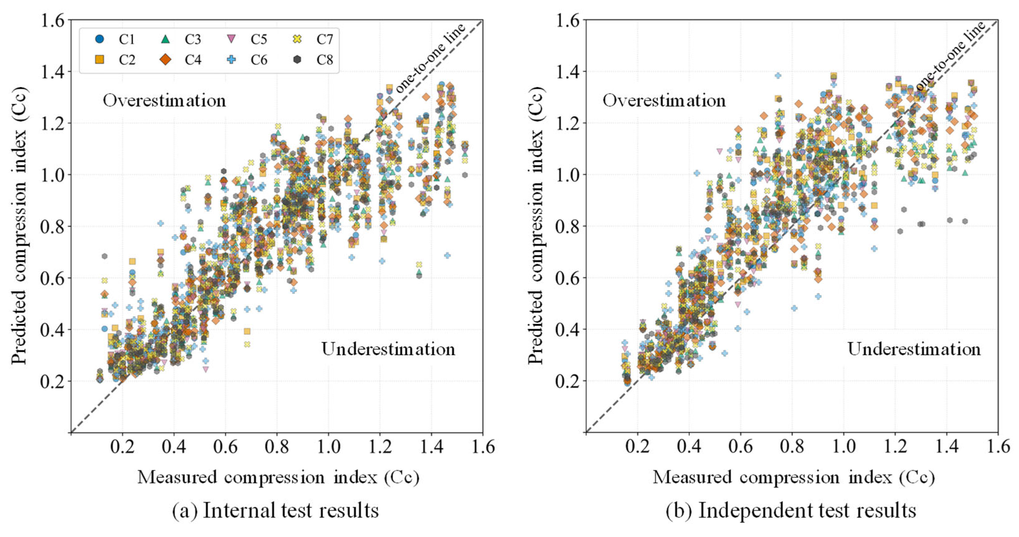
Figure 5 compares the measured Cc values with predictions obtained from the proposed missingness-aware heterogeneous ensemble for the internal and independent test datasets. Prediction accuracy was evaluated using the root mean square error (RMSE), mean absolute error (MAE), mean absolute percentage error (MAPE), and coefficient of determination (R²), defined as follows:

$$\mathrm{R}\mathrm{M}\mathrm{S}\mathrm{E}=\surd [(1/\mathrm{n}){\displaystyle \sum _{i=1}^n}{\left(y_i-\widehat{y_i}\right)}^2]$$

(2)

$$\mathrm{M}\mathrm{A}\mathrm{E}=(1/\mathrm{n}){\displaystyle {\sum }_{i=1}^n}\left|y_i-\widehat{y_i}\right|$$

(3)

$$\mathrm{M}\mathrm{A}\mathrm{P}\mathrm{E}=(100/\mathrm{n}){\displaystyle {\sum }_{i=1}^n}\left|(y_i-\widehat{y_i})/y_i\right|$$

(4)

$$R^2=1-[{\displaystyle {\sum }_{i=1}^n}{\left(y_i-\widehat{y_i}\right)}^2/{\displaystyle {\sum }_{i=1}^n}{\left(y_i-\overline{y}\right)}^2]$$

(5)

where n is the number of observations, y_i and $\widehat{y_i}$ are the measured and predicted Cc values, respectively, and $\overline{y}$ is the mean measured Cc. Lower RMSE, MAE, and MAPE and higher R² indicate better predictive performance.

Figure 5. Measured versus predicted compression index (Cc) across C1–C8 for the proposed model.

As shown in the figure, the predictions generally followed the 1:1 reference line over the measured range, and scatter increased as Cc increased. For the internal-test dataset shown in Figure 5a, the proposed model achieved mean RMSE, MAE, MAPE, and R² values of 0.166, 0.120, 20.19%, and 0.772, respectively, across C1–C8 (Table 9). C2 produced the lowest RMSE (0.153) and highest R² (0.807), closely followed by C1 and C5. C6 was the most difficult internal scenario, with an RMSE of 0.179 and R² of 0.735.

Table 9. Prediction performance of the proposed missingness-aware heterogeneous ensemble.

Case	Prediction Error
	Internal Test				Independent Test
	RMSE	MAE	MAPE	R2	RMSE	MAE	MAPE	R2
C1	0.154	0.109	18.213	0.806	0.172	0.130	20.478	0.737
C2	0.153	0.110	18.899	0.807	0.167	0.129	20.755	0.753
C3	0.173	0.125	20.274	0.755	0.183	0.141	22.317	0.703
C4	0.163	0.117	19.504	0.781	0.173	0.136	21.121	0.736
C5	0.153	0.110	18.744	0.807	0.174	0.130	20.428	0.733
C6	0.179	0.131	22.444	0.735	0.173	0.135	22.821	0.736
C7	0.175	0.127	21.516	0.749	0.187	0.147	22.854	0.689
C8	0.179	0.131	21.943	0.738	0.186	0.144	22.755	0.693
Average	0.166	0.120	20.192	0.772	0.177	0.137	21.691	0.723

For the independent-test dataset, the corresponding mean RMSE, MAE, MAPE, and R² values were 0.177, 0.137, 21.69%, and 0.723, respectively. C2 again produced the lowest RMSE (0.167) and highest R² (0.753), whereas C7 produced the highest RMSE (0.187), MAE (0.147), and MAPE (22.85%) and the lowest R² (0.689).

Compared with the internal-test results, the independent-test mean RMSE and MAE increased by 0.011 and 0.016, respectively, while mean R² decreased from 0.772 to 0.723. MAPE increased by 1.50 percentage points, from 20.19% to 21.69%. For the complete-input scenario C1, R² decreased from 0.806 to 0.737, indicating a measurable spatial-generalization gap even when all six variables were available.

4.2. Performance of Comparative Models

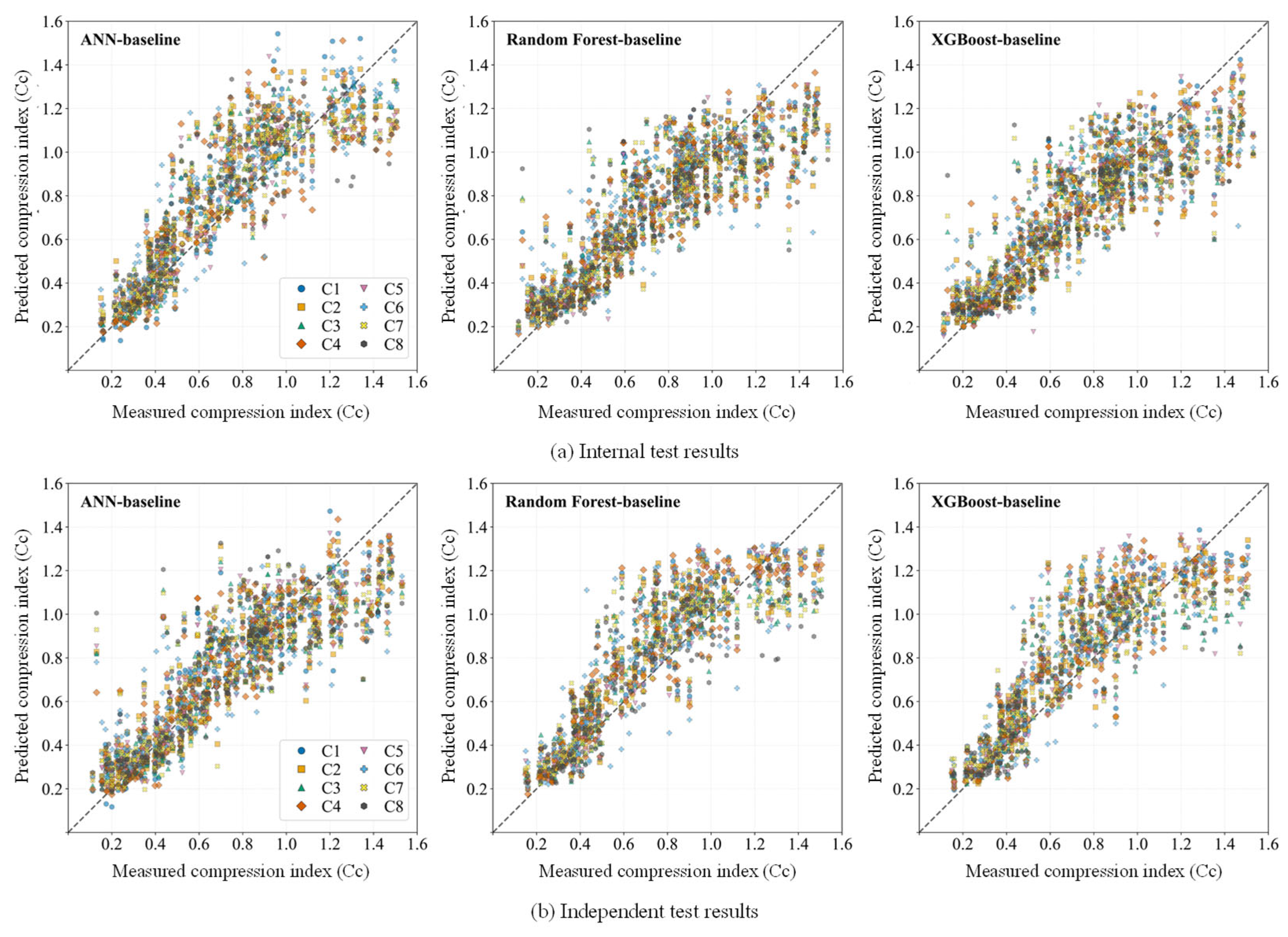
Figure 6 presents the measured and predicted Cc values obtained using the case-specific ANN, RF, and XGBoost baselines. Each baseline was trained independently for C1–C8 using only the variables available in the corresponding scenario. The internal and independent test results are summarized in Table 10 and Table 11, respectively.

Figure 6. Measured versus predicted compression index (Cc) across C1–C8 for the case-specific baselines.

Table 10. Prediction performance of the case-specific ANN, RF, and XGBoost baselines for the internal-test dataset.

Case	Prediction Error
	ANN-Baseline				Random Forest-Baseline				XGBoost-Baseline
	RMSE	MAE	MAPE	R2	RMSE	MAE	MAPE	R2	RMSE	MAE	MAPE	R2
C1	0.164	0.118	20.035	0.779	0.166	0.120	19.847	0.772	0.162	0.114	18.056	0.784
C2	0.166	0.123	21.993	0.773	0.162	0.116	19.147	0.784	0.165	0.119	19.106	0.777
C3	0.181	0.130	21.235	0.731	0.184	0.133	22.018	0.723	0.181	0.132	21.491	0.731
C4	0.164	0.119	19.551	0.779	0.171	0.124	20.152	0.759	0.173	0.125	19.923	0.754
C5	0.162	0.119	21.065	0.783	0.162	0.117	19.147	0.783	0.160	0.115	18.279	0.790
C6	0.193	0.147	26.670	0.695	0.188	0.138	23.769	0.711	0.191	0.146	25.544	0.699
C7	0.187	0.137	23.610	0.713	0.185	0.135	22.735	0.719	0.186	0.136	23.236	0.716
C8	0.190	0.137	23.609	0.703	0.191	0.139	23.463	0.700	0.195	0.143	23.785	0.688
Average	0.176	0.129	22.221	0.745	0.176	0.128	21.285	0.744	0.177	0.129	21.177	0.742

Table 11. Prediction performance of the case-specific ANN, RF, and XGBoost baselines in the independent test.

Case	Prediction Error
	ANN-Baseline				Random Forest-Baseline				XGBoost-Baseline
	RMSE	MAE	MAPE	R2	RMSE	MAE	MAPE	R2	RMSE	MAE	MAPE	R2
C1	0.174	0.129	20.158	0.732	0.169	0.131	20.609	0.746	0.179	0.134	20.831	0.717
C2	0.187	0.146	23.266	0.690	0.172	0.133	21.293	0.739	0.176	0.134	21.296	0.727
C3	0.179	0.136	21.964	0.716	0.186	0.144	22.414	0.694	0.201	0.150	23.047	0.644
C4	0.203	0.156	23.260	0.634	0.174	0.136	21.199	0.731	0.177	0.136	21.030	0.723
C5	0.181	0.140	21.824	0.710	0.172	0.131	20.997	0.737	0.187	0.141	21.894	0.691
C6	0.186	0.145	25.198	0.694	0.193	0.150	25.588	0.669	0.192	0.147	24.860	0.676
C7	0.190	0.147	23.091	0.682	0.193	0.148	23.464	0.671	0.185	0.144	23.535	0.698
C8	0.196	0.149	23.241	0.661	0.189	0.144	22.481	0.684	0.182	0.142	22.484	0.706
Average	0.187	0.144	22.750	0.690	0.181	0.139	22.255	0.709	0.185	0.141	22.372	0.698

For the internal-test dataset, ANN, RF, and XGBoost produced mean RMSE values of 0.176, 0.176, and 0.177 and mean R² values of 0.745, 0.744, and 0.742, respectively. Their mean MAE values were approximately 0.128–0.129, while mean MAPE ranged from 21.18% for XGBoost to 22.22% for ANN. The similarity of these average values indicates that no single baseline learner was uniformly optimal across the missing-input scenarios.

For the independent-test dataset, RF provided the strongest mean baseline performance, with RMSE, MAE, MAPE, and R² values of 0.181, 0.139, 22.26%, and 0.709, respectively (Table 11). ANN yielded the highest mean RMSE (0.187) and lowest mean R² (0.690), while XGBoost was intermediate with an RMSE of 0.185 and R² of 0.698.

To prevent test-set information from influencing the selection of the representative empirical benchmark, all 15 empirical correlations were first evaluated using the same 124 complete-input validation specimens. The correlations were ordered according to validation RMSE, which was used to select the representative empirical benchmark. MAE, MAPE, and R² were retained as complementary performance measures to provide a broader description of prediction accuracy. For descriptive comparison, the correlations were ranked separately by RMSE, MAE, and MAPE in ascending order. The three metric-specific ranks were assigned equal weight and averaged to obtain a supplementary mean rank. R² was excluded from this calculation because its ranking is mathematically equivalent to the RMSE ranking for a fixed dataset. The supplementary mean rank was reported descriptively and was not used for benchmark selection. As summarized in Table 12, EC-4 achieved the lowest unrounded validation RMSE of 0.1619, followed closely by EC-5 with an RMSE of 0.1621. EC-4 was therefore selected as the representative empirical benchmark before evaluation on the internal and independent test sets.

Table 12. Validation performance of the 15 empirical correlations ordered by RMSE.

RMSE Rank (Mean Rank)	ID	Inputs	Prediction Error
			RMSE	MAE	MAPE	R2
1 (1.33)	EC-4	wn	0.1619	0.128	23.32	0.763
2 (3.00)	EC-5	eo	0.1621	0.127	25.90	0.762
3 (5.67)	EC-9	LL	0.2023	0.158	29.49	0.630
4 (4.67)	EC-12	eo, wn	0.2053	0.162	25.22	0.619
5 (5.67)	EC-2	wn	0.2062	0.161	26.14	0.616
6 (4.67)	EC-11	wn, LL	0.2116	0.164	23.83	0.595
7 (5.67)	EC-15	eo, wn, LL	0.2142	0.168	24.53	0.586
8 (6.67)	EC-13	eo, LL	0.2150	0.170	24.85	0.582
9 (8.33)	EC-6	eo	0.2224	0.176	26.01	0.553
10 (12.33)	EC-10	wn, LL	0.2285	0.199	45.18	0.528
11 (10.00)	EC-1	wn	0.2332	0.183	26.41	0.509
12 (11.00)	EC-3	wn	0.2494	0.198	27.58	0.438
13 (13.00)	EC-14	eo, LL	0.2928	0.235	31.31	0.225
14 (13.33)	EC-8	LL	0.3029	0.236	31.07	0.171
15 (14.67)	EC-7	eo	0.3207	0.262	34.44	0.071

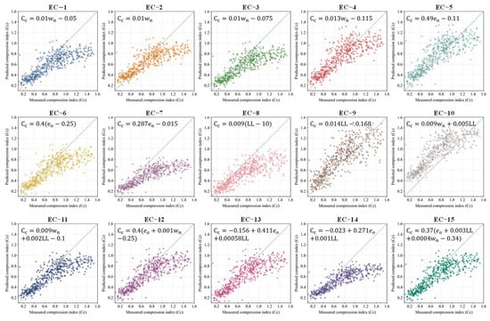
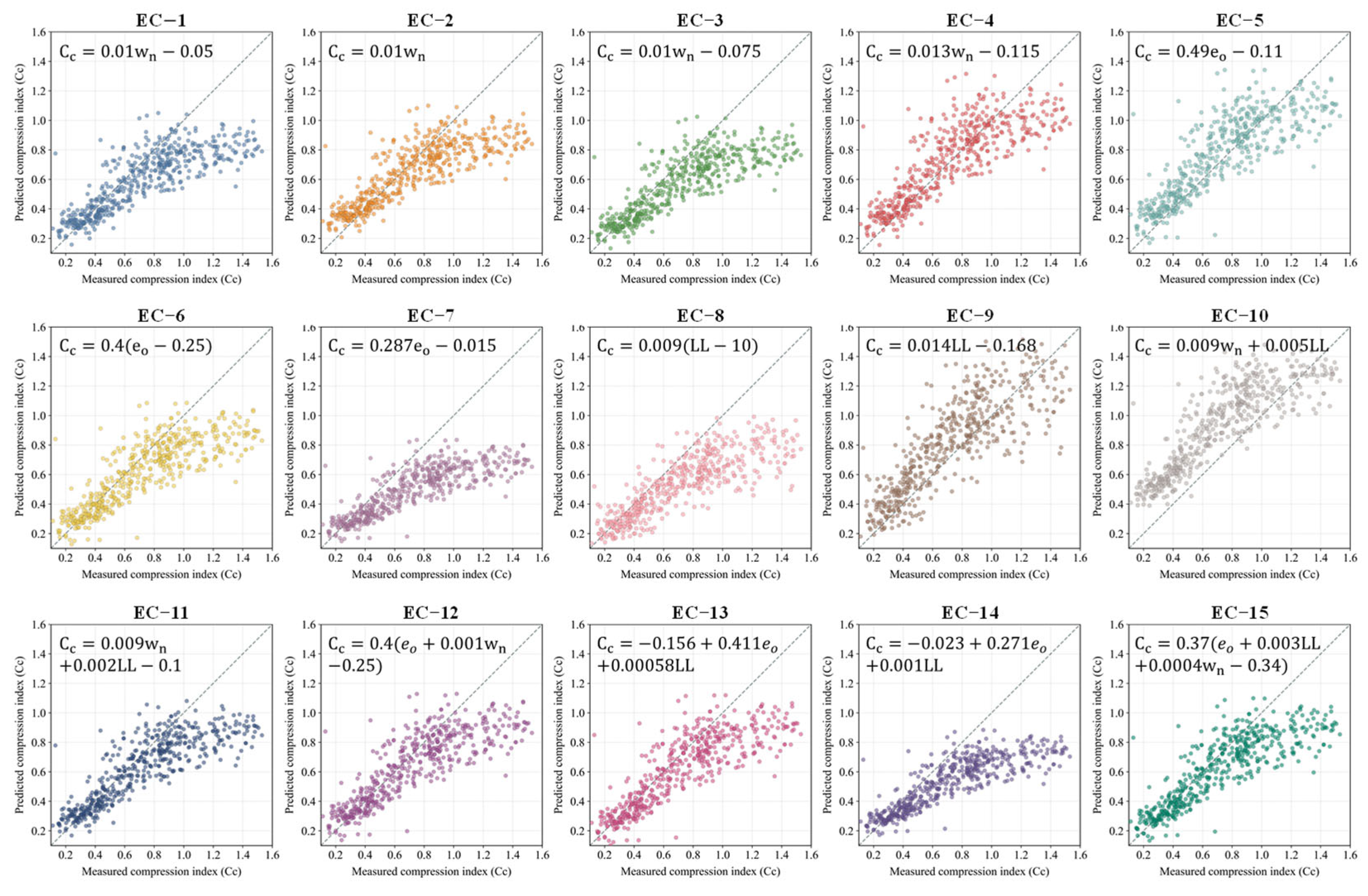
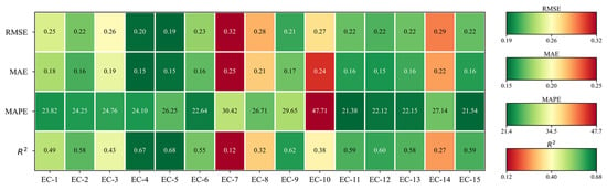
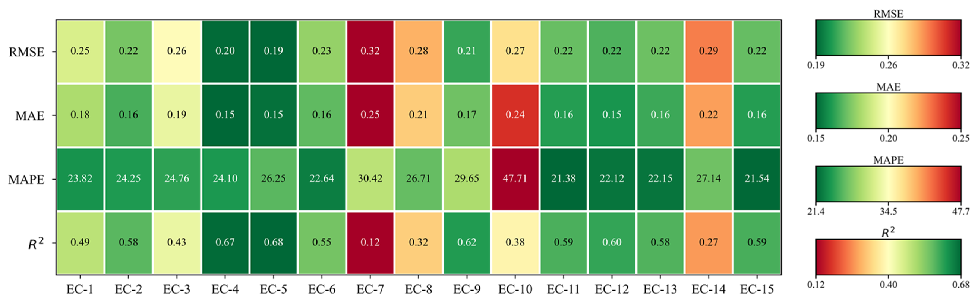
After the representative empirical benchmark had been selected, the test-set results for all 15 equations were examined descriptively in Figure 7 and Figure 8. Figure 7 shows the measured-versus-predicted distributions for the combined internal- and independent-test datasets, whereas Figure 8 compares the corresponding RMSE, MAE, MAPE, and R² values. These test-set results were not used to select EC-4 but were retained to provide a complete out-of-sample comparison of the empirical correlations. The distributions showed marked differences in scatter and deviation from the 1:1 line across the equations. Distinct prediction patterns were also observed among correlations based on an individual soil parameter. The metric comparison further showed that equations with relatively low RMSE and high R² did not necessarily produce the lowest MAE or MAPE.

Figure 7. Measured versus predicted compression index (Cc) for the 15 empirical correlations using the combined internal- and independent-test datasets.

Figure 8. Performance of the 15 empirical correlations across four evaluation metrics using the combined internal- and independent-test datasets.

In the combined test-set evaluation, EC-5 achieved the lowest RMSE of 0.194 and the highest R² of 0.680, whereas EC-4 yielded slightly lower MAE and MAPE values of 0.145 and 24.099%, respectively. EC-12, EC-15, and EC-11 produced lower MAPE values than EC-4 and EC-5 but had higher RMSE and lower R² values. These differences demonstrate that the relative test-set performance depended on the selected metric. Nevertheless, the representative empirical benchmark remained EC-4 because its selection had been determined exclusively from the validation RMSE rather than retrospectively from the internal- or independent-test results.

4.3. Comparative Performance, Uncertainty, and Error Characteristics

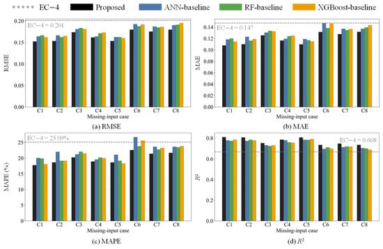
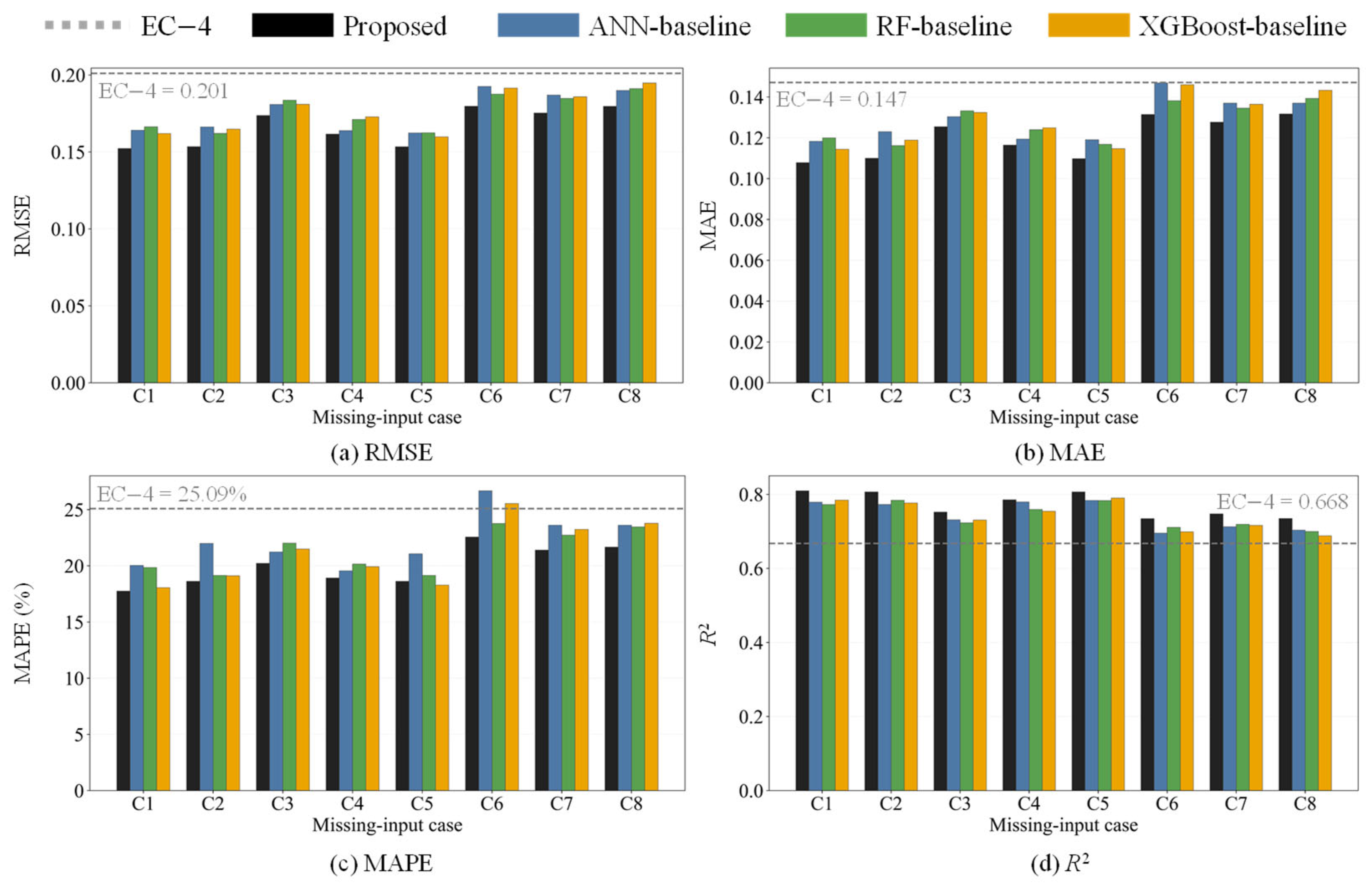
Figure 9 and Figure 10 compare the proposed model with the case-specific machine-learning baselines and EC-4 across the eight missing-input scenarios. Because EC-4 requires w_n, it was evaluated independently of the scenario-specific input configurations. In the internal test shown in Figure 9, the proposed model produced more favorable point-estimate metric values than ANN and RF in all 32 case-metric comparisons. It also produced more favorable values than XGBoost in 30 of 32 comparisons, with the MAPE results for C1 and C5 as the only exceptions.

Figure 9. Comparison of the proposed model with the case-specific baselines and EC-4 in the internal test.

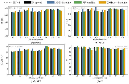
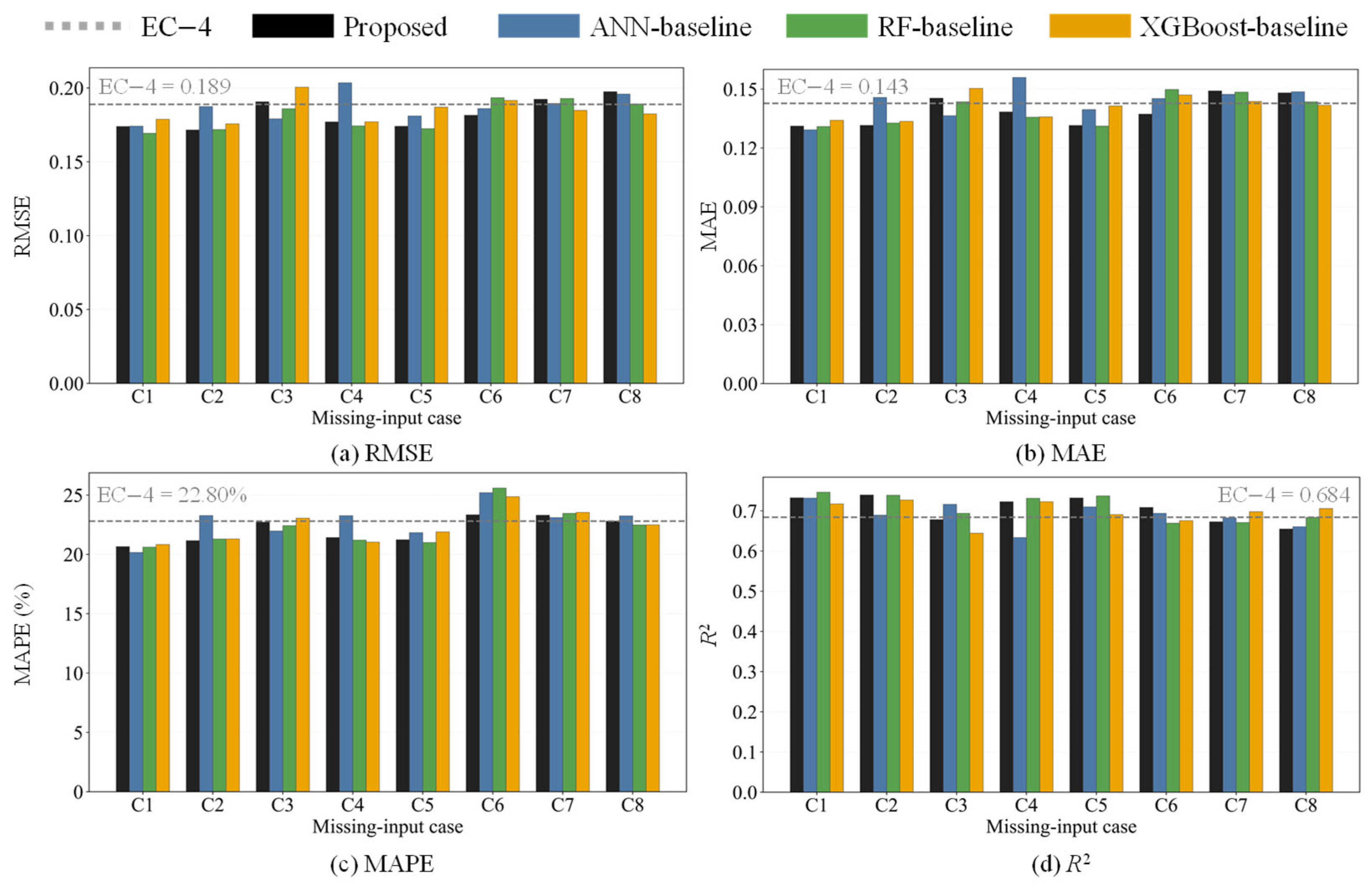
Figure 10. Comparison of the proposed model with the case-specific baselines and EC-4 in the independent test.

This broad internal-test pattern became less consistent at the independent sites shown in Figure 10. The proposed model produced more favorable point-estimate metric values than ANN and RF in 25 of 32 comparisons for each baseline and than XGBoost in 23 comparisons. These counts describe point-estimate differences and should not be interpreted as evidence of uniform superiority. The greater variation in model ranking reflected the more demanding evaluation at sites excluded from model development. Nevertheless, the unified framework remained competitive across all eight missing-input configurations.

The scenario-level results further showed why performance should be considered in relation to input identity rather than input count alone. C2 produced the lowest or near-lowest errors in both tests, although its small difference from C1 does not indicate that removing w_n improved prediction. This distinction was reinforced by C7 and C8. Both scenarios retained two inputs, yet C7 consistently produced larger errors. The pattern agreed with the correlation analysis in Figure 3, where w_n and LL as well as PI and e_o showed stronger relationships with Cc than CF and Act.

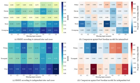
Figure 11 illustrates the site-wise RMSE of the proposed model together with its difference from the best case-specific baseline at each independent site. The site-wise presentation was used to prevent the pooled independent-test metrics from obscuring performance differences among sites with unequal sample sizes. The best case-specific baseline was defined retrospectively for each site and scenario as the model with the lowest test-set RMSE among ANN, RF, and XGBoost. It was therefore used only as a descriptive oracle benchmark and not as a deployable model-selection rule. The results should be interpreted as site-specific comparisons rather than as evidence of uniform performance across unseen geological regions.

Figure 11. Site-wise RMSE and its difference from the best case-specific baseline.

Negative values in Figure 11b,d favor the proposed model, whereas positive values favor the baseline. In the internal test, Mokpo and Incheon showed similar RMSE ranges of 0.075–0.115 and 0.076–0.101. In contrast, Gwangyang produced the highest range of 0.187–0.223. At the independent sites, RMSE ranged from 0.131–0.171 for Pyeongtaek and 0.139–0.211 for Pohang, while Ulsan showed the highest independent-test range of 0.195–0.242.

These site-level differences were accompanied by changes in the most difficult missing-input scenario. C6 produced the highest RMSE at Mokpo and Gunsan as well as Incheon and Gwangyang. At Busan, the highest value occurred under C3 and C8. A different pattern emerged at the independent sites. C7 was most difficult for Pohang, while C6 and C8 were most difficult for Pyeongtaek and Ulsan. Thus, no scenario produced the highest error at every site.

The location dependence also appeared in comparisons with the best case-specific baseline. In the internal test, the largest RMSE reductions were observed at Busan under C5 (−0.032) and C1 (−0.026). Gwangyang under C8 showed a smaller reduction of −0.020. In the independent test, the largest reductions occurred at Pohang under C3 (−0.031) and C2 (−0.021). However, the baseline performed better at Ulsan under C3 (+0.035) and C8 (+0.026). It also performed better at Pohang under C7 (+0.019).

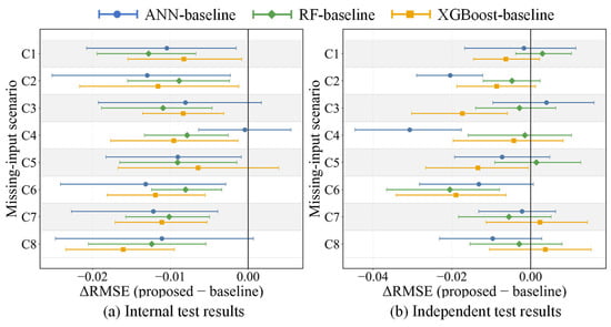
Figure 12 evaluates the stability of the model comparisons through bootstrap estimates of ΔRMSE. Uncertainty was quantified through paired specimen-level bootstrap resampling. For each split, scenario, and baseline, the proposed and baseline predictions for the same specimen were resampled together with replacement. A total of 5000 bootstrap samples were generated using random seed 20260721. Each sample contained 282 specimens for the internal test or 215 specimens for the independent test. The 2.5th and 97.5th percentiles of the resulting RMSE differences defined the 95% confidence interval. ΔRMSE was calculated by subtracting the RMSE of each baseline from that of the proposed model. Negative values therefore favor the proposed model, and an interval entirely below zero indicates a stable RMSE reduction under resampling. Because individual specimens were used as the resampling units, these intervals quantify specimen-level uncertainty conditional on the fixed composition of the observed test sites. They do not account for clustering within sites or boreholes and should not be interpreted as estimates of between-site uncertainty for transfer to an arbitrary new geological region.

Figure 12. Bootstrap estimates and 95% confidence intervals of ΔRMSE between the proposed model and the case-specific baselines.

In the internal test, 20 of the 24 confidence intervals remained below zero. The remaining four intervals crossed zero. All three baseline comparisons were below zero under C1 and C2 as well as C6 and C7. The independent test retained the same overall tendency but showed greater uncertainty. The bootstrap mean ΔRMSE was negative in 19 of the 24 comparisons, indicating that the proposed model generally tended to produce lower RMSE than the baselines. Among these comparisons, six confidence intervals remained entirely below zero in the unadjusted exploratory analysis. The remaining 18 intervals included zero and therefore did not consistently support an RMSE difference under specimen-level resampling. Notably, no confidence interval remained entirely above zero. These results describe uncertainty within the fixed test datasets and should not be interpreted as confirmatory evidence of superiority or as an estimate of between-site transfer uncertainty.

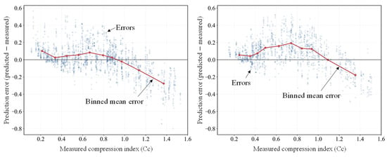
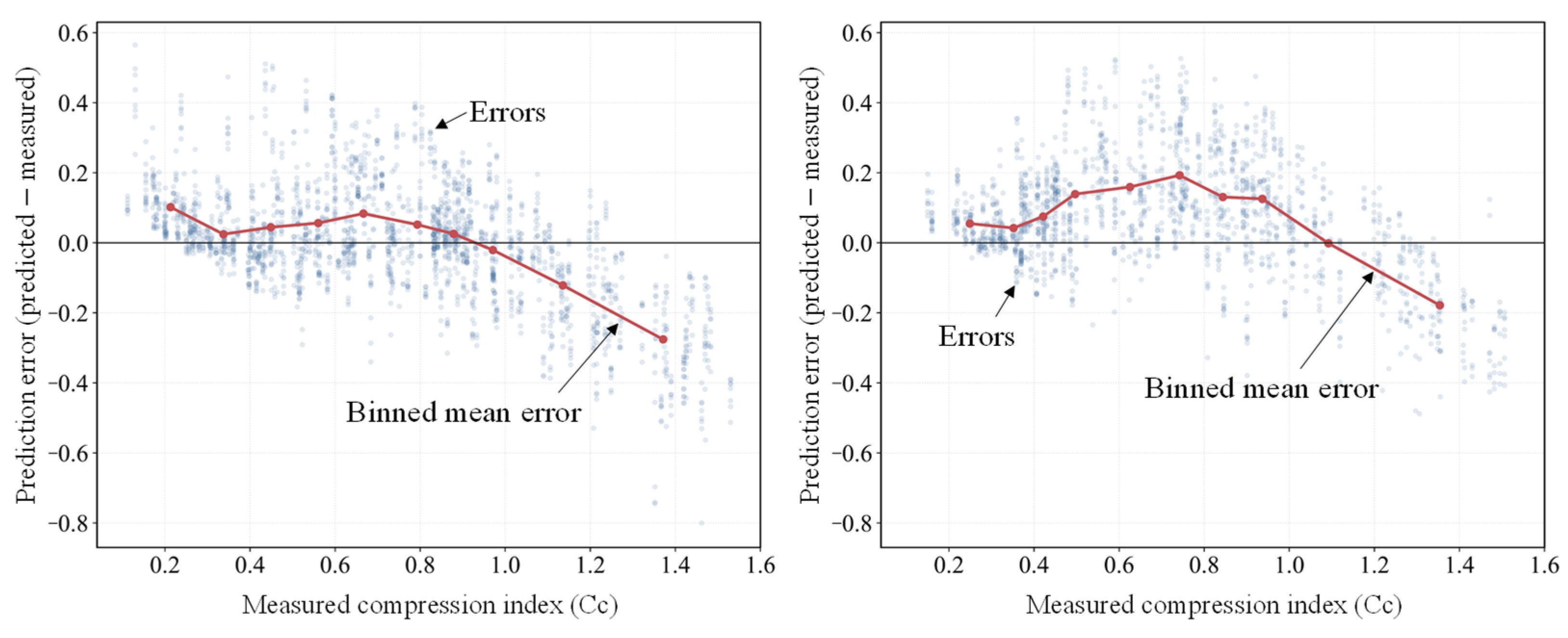
Figure 13 shows how the signed prediction error changed with measured Cc. Scenario-specific prediction rows were pooled across C1–C8 within each test split. Measured Cc was divided into ten equal-frequency bins separately for the internal and independent tests, and the mean signed error was calculated in each bin. The signed error was defined as predicted Cc minus measured Cc. Although individual predictions were dispersed around zero, the binned mean followed a nonlinear trend. Mean error was generally positive across the low-to-intermediate Cc range. It then became negative as measured Cc approached and exceeded approximately 1.0.

Figure 13. Signed prediction error as a function of measured compression index (Cc).

The negative trend strengthened toward the upper end of the measured range and indicated systematic underprediction for highly compressible specimens. In the independent test, the positive mean error was also more pronounced in the intermediate range before crossing zero. This magnitude-dependent pattern was not apparent from the average performance metrics alone. Accordingly, the average performance metrics should not be interpreted as evidence of uniform accuracy across the measured Cc range.

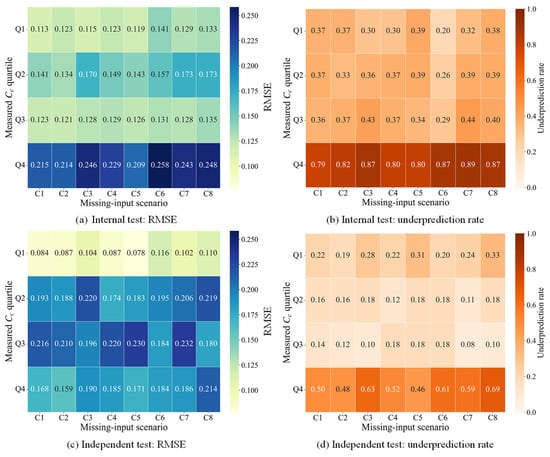
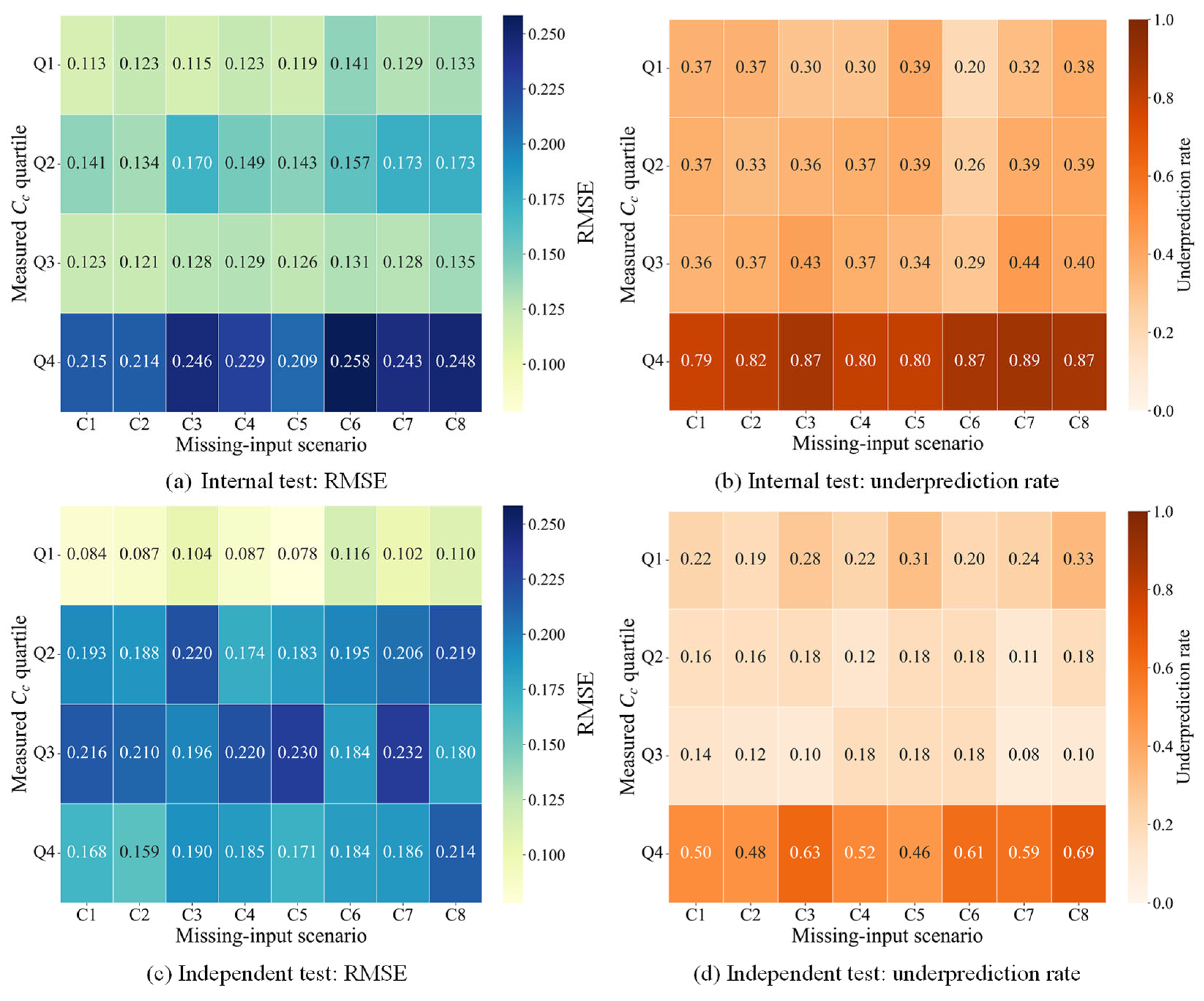
Figure 14 examines the residual pattern across measured-Cc quartiles. Measured Cc was divided into quartiles separately within the internal and independent tests, and the resulting boundaries were applied consistently to C1–C8 within each split. RMSE and underprediction rate were calculated separately for each scenario and quartile. Underprediction was defined as a prediction lower than the corresponding measured Cc.

Figure 14. RMSE and underprediction rate across measured-Cc quartiles and incomplete-input scenarios.

In the internal test, Q4 produced the largest RMSE in every scenario with values of 0.209–0.258. Its underprediction rate ranged from 0.79 to 0.89, whereas Q1–Q3 showed RMSE values of 0.075–0.173 and rates of 0.20–0.44. The independent test showed a less uniform RMSE pattern because Q2 and Q3 were also difficult under several scenarios. Even so, Q4 retained the highest underprediction rate at 0.46–0.69. The corresponding rates for Q1–Q3 were 0.08–0.33, confirming that high-Cc specimens were more frequently underestimated at the independent sites. These quartile-specific results provide magnitude-conditioned error and directional-bias information but do not constitute a formal calibration or prediction-interval analysis. This systematic high-Cc underprediction may lead to unconservative preliminary settlement estimates for highly compressible soils.

4.4. Discussion

Taken together, the scenario-level results show that the identity of the available inputs mattered more than their number. C2 performed as well as or slightly better than C1 for several metrics, but this small difference does not imply that removing water content improved prediction. Instead, LL and PI together with e_o may have provided overlapping information within the present database. The contrast between C7 and C8 supports this interpretation. Although both scenarios contained two inputs, they produced clearly different prediction errors.

The importance of input identity was accompanied by a clear spatial effect. The location-based split provided a more spatially separated evaluation than a random specimen-level split because the independent sites were excluded from model development. Performance declined in the independent test, and RMSE varied substantially among sites. These site-level differences were associated with variation in prediction accuracy. Ulsan was the most challenging independent site, whereas Pyeongtaek generally produced lower RMSE values. The site-specific reversals against the best baseline further show that no model dominated under every geological condition.

Because the training, validation, and internal-test sets were partitioned at the specimen level, borehole-level dependence may remain in the internal evaluation and could produce more favorable performance than a borehole-grouped split. This limitation does not apply to the independent-site test because Pyeongtaek, Pohang, and Ulsan, including all boreholes and specimens from these sites, were completely excluded from model development.

The site-specific sample sizes were imbalanced, with Gwangyang and Busan together accounting for approximately 59.7% of the complete database. Because the models were trained using equally weighted specimens, the property distributions of these major model-development sites may have exerted greater influence on model fitting. Although site identifiers were not used as model inputs, an indirect site-related influence cannot be excluded because the soil-property distributions differed among locations. Site-balanced training was not adopted because it would assign greater weight to individual specimens from smaller sites and could amplify sampling variability. Future studies should compare specimen-weighted and site-balanced training across rotating site-based partitions.

The spatial-transfer results are specific to the predefined combination of Pyeongtaek, Pohang, and Ulsan. In particular, the Pohang result, based on 22 specimens, should be interpreted as an exploratory site-level assessment with limited precision. Moreover, the paired bootstrap confidence intervals reflect specimen-level uncertainty within the fixed test-site composition and do not quantify uncertainty associated with transfer to a new geological region. Because only three independent sites were available, between-site uncertainty could not be estimated precisely. The multiple scenario- and baseline-specific intervals were unadjusted for multiplicity and should therefore be interpreted as exploratory. Rotating leave-one-site-out or leave-multiple-sites-out analysis would provide a broader assessment of sensitivity to site selection and should be considered in future research. Future multi-site studies should also apply grouped or hierarchical resampling across a larger number of independent sites and boreholes.

The present findings agree with prior evidence that ensemble learning can improve Cc prediction. Diaz and Spagnoli [26] combined tree learners in a global super-learner framework, while Ge et al. [27] reported that stacking outperformed individual learners in a 1080-sample database. However, Ge et al. addressed incomplete records through K-nearest-neighbor imputation, and Diaz and Spagnoli provided separate symbolic equations for reduced input sets. Pang et al. [36] more directly incorporated geographical information and feature missingness. The present framework differed by encoding availability indicators within one shared model and testing transfer to three sites excluded from model development. Its less stable advantage at those sites reinforces the need for location-based validation when spatial generalization is claimed.

The spatial variation was not the only limitation revealed by the detailed error analyses. Residuals became more negative as measured Cc increased, and Q4 showed the highest underprediction rate in both tests. This pattern may reflect regression toward the center of the training distribution because the upper tail was sparsely represented in the training data (Cc ≥ 1.2: 87 of 903 specimens, 9.6%). Such underestimation can lead to unconservative settlement screening. Predictions for highly compressible clays should therefore be verified through targeted laboratory testing. Future studies should evaluate formal calibration and develop prediction intervals with conditional coverage assessed across Cc ranges, input scenarios, and independent sites.

The bootstrap analysis places these average trends in a more cautious context. Most internal-test intervals supported a stable RMSE reduction, whereas many independent-test intervals crossed zero. The proposed model therefore achieved favorable average accuracy without showing a uniform advantage at unseen sites. The independent-test point estimates generally favored the proposed model, but most corresponding confidence intervals did not exclude zero. This distinction defines its appropriate practical role. The model can support preliminary screening, but it should not replace site-specific characterization.

These findings also define the present scope of application. The study considered eight predefined missing-input scenarios and three independent sites, whereas field datasets may contain irregular missingness or measurement errors. Such datasets may also include input combinations not represented by C1–C8. Further work should therefore evaluate the framework in additional geological regions and under irregular specimen-level missingness and previously unseen input combinations. Improved calibration for high-Cc soils should also be examined together with prediction intervals for individual estimates.

A further consideration concerns the comparison design. The present analysis reflects the practical distinction between one shared framework and multiple case-specific models. Joint training across C1–C8 may have allowed the proposed framework to use information shared among the input scenarios. The proposed framework and the case-specific baselines differed in model structure, model count, joint versus separate training, and optimization budget. Consequently, the observed performance differences characterize the complete implemented systems and cannot be attributed exclusively to zero masking, availability indicators, shared training, ANN seed ensembling, heterogeneous learners, or optimized blending. The present comparison was therefore not intended as a controlled component-attribution study. Future studies should conduct matched-budget ablation experiments comparing zero masking without availability indicators, shared training without availability indicators, a shared model with availability indicators but without heterogeneous blending, the best single shared learner, an equal-weight ensemble, case-specific ensembles of comparable complexity, and the complete framework. A separate feature-ablation analysis is also needed to determine whether the derived activity feature provides incremental predictive value beyond PI and CF.

The model-selection procedure repeatedly used the same fixed set of 124 validation specimens across hyperparameter optimization, early stopping, ANN seed-weight determination, and global blending. Although the internal and independent test sets remained completely excluded from these procedures, the repeated adaptive use of the same validation specimens may have favored configurations tailored to this particular validation set. Accordingly, validation performance was not interpreted as an independent estimate of final predictive performance, and the conclusions were based on the untouched internal and independent test results. Variability associated with ANN initialization was partially addressed through the five-seed ANN ensemble, whereas variability across alternative validation sets and site partitions was not examined in the present study. Future studies should examine the stability of the selected configurations through site-aware nested or repeated validation and repeated training with additional random seeds.

5. Conclusions

This study developed a missingness-aware heterogeneous ensemble for predicting Cc under predefined incomplete-input conditions. The analysis used 1524 marine-clay specimens from eight coastal sites and considered eight predefined missing-input scenarios. Masked and scaled soil variables were combined with explicit availability indicators, which allowed one model structure to process every scenario. Validation-derived global weights then combined the ANN seed ensemble with four tree-based learners.

The proposed model achieved mean RMSE values of 0.166 and 0.177 in the internal and independent tests, with corresponding R² values of 0.772 and 0.723. In the internal test, it produced more favorable metric values than ANN and RF in all 32 case-metric comparisons and than XGBoost in 30 comparisons. The corresponding point-estimate differences were less consistent in the independent test, where the proposed model produced more favorable values in 25 comparisons against each of ANN and RF and in 23 comparisons against XGBoost. However, only six of the 24 independent-test bootstrap confidence intervals remained entirely below zero, indicating that the RMSE reductions were not consistently supported across the comparisons. These comparisons characterize the performance of the complete implemented framework and do not establish either uniform superiority over the baselines or the contribution of any individual framework component.

Beyond the average performance differences, prediction accuracy depended on both the available soil properties and the test location. Input count alone did not explain the scenario-level differences, and Ulsan produced the largest errors among the independent sites. The residual and quartile analyses also revealed systematic underprediction at high measured Cc. Accordingly, the framework is intended for preliminary Cc screening and should not replace laboratory consolidation testing. Predictions for highly compressible soils require laboratory confirmation because underprediction may lead to unconservative settlement estimates.

Overall, the proposed framework handled all eight predefined input scenarios within one shared ensemble framework, whereas the baselines required 24 case-specific models. Its broader use will require validation in additional geological regions as well as tests with irregular specimen-level missingness and previously unseen input combinations.

References

- Hong, S.; Kim, S.R. Physics-informed neural networks for back-analysis and consolidation settlement prediction using field measurements. Acta Geotech. 2026, 21, 2309–2342. [Google Scholar] [CrossRef] [Scilit]
- Zhou, P.; Dai, F.; Yang, S.; Liu, Y.; Yan, Z.; Wei, M. Long-term cyclic performance of offshore jacked piles in structured clays: Insights from model testing. Mar. Struct. 2025, 101, 103769. [Google Scholar] [CrossRef] [Scilit]
- Terzaghi, K.; Peck, R.B.; Mesri, G. Soil Mechanics in Engineering Practice, 3rd ed.; John Wiley & Sons: New York, NY, USA, 1996. [Google Scholar]
- Park, H.I.; Lee, S.R. Evaluation of the compression index of soils using an artificial neural network. Comput. Geotech. 2011, 38, 472–481. [Google Scholar] [CrossRef] [Scilit]
- Mayne, P.W.; Kootahi, K. Index test method for estimating the effective preconsolidation stress in clay deposits. J. Geotech. Geoenviron. Eng. 2016, 142, 04016044. [Google Scholar] [CrossRef] [Scilit]
- Jayalekshmi, S.; Elamathi, V. A review on correlations for consolidation characteristics of various soils. IOP Conf. Ser. Mater. Sci. Eng. 2020, 1006, 012007. [Google Scholar] [CrossRef] [Scilit]
- Azzouz, A.S.; Krizek, R.J.; Corotis, R.B. Regression analysis of soil compressibility. Soils Found. 1976, 16, 19–29. [Google Scholar] [CrossRef] [Scilit]
- Koppula, S.D. Statistical estimation of compression index. Geotech. Test. J. 1981, 4, 68–73. [Google Scholar] [CrossRef] [Scilit]
- Rendon-Herrero, O. Universal compression index equation. J. Geotech. Eng. Div. 1980, 106, 1179–1200. [Google Scholar] [CrossRef] [Scilit]
- Rendon-Herrero, O. Closure to universal compression index equation. J. Geotech. Eng. 1983, 109, 755–761. [Google Scholar] [CrossRef] [Scilit]
- Al-Khafaji, A.W.N.; Andersland, O.B. Equations for compression index approximation. J. Geotech. Eng. 1992, 118, 148–153. [Google Scholar] [CrossRef] [Scilit]
- Sridharan, A.; Nagaraj, H.B. Compressibility behaviour of remoulded, fine-grained soils and correlation with index properties. Can. Geotech. J. 2000, 37, 712–722. [Google Scholar] [CrossRef]
- Bae, W.; Heo, T.Y. Prediction of compression index using regression analysis of transformed variables method. Mar. Georesour. Geotechnol. 2011, 29, 76–94. [Google Scholar] [CrossRef] [Scilit]
- Spagnoli, G.; Shimobe, S. Statistical analysis of some correlations between compression index and Atterberg limits. Environ. Earth Sci. 2020, 79, 532. [Google Scholar] [CrossRef] [Scilit]
- Shimobe, S.; Spagnoli, G. A general overview on the correlation of compression index of clays with some geotechnical index properties. Geotech. Geol. Eng. 2022, 40, 3689–3708. [Google Scholar] [CrossRef] [Scilit]
- Yoon, G.L.; Kim, B.T.; Jeon, S.S. Empirical correlations of compression index for marine clay from regression analysis. Can. Geotech. J. 2004, 41, 1213–1221. [Google Scholar] [CrossRef] [Scilit]
- Kalantary, F.; Kordnaeij, A. Prediction of compression index using artificial neural network. Sci. Res. Essays 2012, 7, 2835–2848. [Google Scholar] [CrossRef] [Scilit]
- Kurnaz, T.F.; Kaya, Y. The comparison of the performance of ELM, BRNN, and SVM methods for the prediction of compression index of clays. Arab. J. Geosci. 2018, 11, 779. [Google Scholar] [CrossRef] [Scilit]
- Saisubramanian, R.; Murugaiyan, V. Prediction of compression index of marine clay using artificial neural network and multilinear regression models. J. Soft Comput. Civ. Eng. 2021, 5, 114–124. [Google Scholar]
- Asteris, P.G.; Mamou, A.; Ferentinou, M.; Tran, T.T.; Zhou, J. Predicting clay compressibility using a novel manta ray foraging optimization-based extreme learning machine model. Transp. Geotech. 2022, 37, 100861. [Google Scholar] [CrossRef] [Scilit]
- Kim, M.; Senturk, M.A.; Tan, R.K.; Ordu, E.; Ko, J. Deep learning approach on prediction of soil consolidation characteristics. Buildings 2024, 14, 450. [Google Scholar] [CrossRef] [Scilit]
- Uzer, A.U. Accurate prediction of compression index of normally consolidated soils using artificial neural networks. Buildings 2024, 14, 2688. [Google Scholar] [CrossRef] [Scilit]
- Mamudur, K.; Kattamuri, M.R. Application of boosting-based ensemble learning method for the prediction of compression index. J. Inst. Eng. Ser. A 2020, 101, 577–587. [Google Scholar] [CrossRef] [Scilit]
- Zhang, P.; Yin, Z.Y.; Jin, Y.F.; Chan, T.H.T.; Gao, F.P. Intelligent modelling of clay compressibility using hybrid meta-heuristic and machine learning algorithms. Geosci. Front. 2021, 12, 441–452. [Google Scholar] [CrossRef] [Scilit]
- Tsang, L.; He, B.; Ghorbani, A.; Khatami, S.M.H. Tree-based techniques for predicting the compression index of clayey soils. J. Soft Comput. Civ. Eng. 2023, 7, 52–67. [Google Scholar]
- Diaz, E.; Spagnoli, G. A super-learner machine learning model for a global prediction of compression index in clays. Appl. Clay Sci. 2024, 249, 107239. [Google Scholar] [CrossRef] [Scilit]
- Ge, Q.; Xia, Y.; Shu, J.; Li, J.; Sun, H. Explainable ensemble learning approaches for predicting the compression index of clays. J. Mar. Sci. Eng. 2024, 12, 1701. [Google Scholar] [CrossRef] [Scilit]
- Yoo, B.S.; Han, J.T.; Park, H.I.; Yang, E. Prediction of compression index using diverse regression models and variable combinations: Insight from a large geotechnical information database. J. Geotech. Geoenviron. Eng. 2026, 152, 04026039. [Google Scholar] [CrossRef] [Scilit]
- Dai, F.; Gai, W.; Yang, S.; Wei, M.; Liu, Y.; Zhou, P. Machine learning-driven multi-objective optimization and dynamic performance prediction of geopolymer concrete. J. Clean. Prod. 2026, 540, 147501. [Google Scholar] [CrossRef] [Scilit]
- Nguyen, V.Q.; Tran, V.L.; Nguyen, D.D.; Sadiq, S.; Park, D. Novel hybrid MFO-XGBoost model for predicting the racking ratio of rectangular tunnels subjected to seismic loading. Transp. Geotech. 2022, 37, 100878. [Google Scholar] [CrossRef] [Scilit]
- Won, M.S.; Sadiq, S.; Joung, Y.S.; Kim, H.J. GEP-based empirical models for estimation of soil nail bond strength in weathered soil. KSCE J. Civ. Eng. 2025, 29, 100115. [Google Scholar] [CrossRef] [Scilit]
- Won, M.S.; Sadiq, S.; Wang, J.B.; Gao, Y.C. Predicting slope stability potential failure surface using machine learning algorithms. Arab. J. Geosci. 2025, 18, 24. [Google Scholar] [CrossRef] [Scilit]
- Schafer, J.L.; Graham, J.W. Missing data: Our view of the state of the art. Psychol. Methods 2002, 7, 147–177. [Google Scholar] [CrossRef]
- Roberts, D.R.; Bahn, V.; Ciuti, S.; Boyce, M.S.; Elith, J.; Guillera-Arroita, G.; Hauenstein, S.; Lahoz-Monfort, J.J.; Schroder, B.; Thuiller, W.; et al. Cross-validation strategies for data with temporal, spatial, hierarchical, or phylogenetic structure. Ecography 2017, 40, 913–929. [Google Scholar] [CrossRef] [Scilit]
- Lee, S.; Kang, J.; Kim, J.; Baek, W.; Yoon, H. A study on developing a model for predicting the compression index of the South Coast clay of Korea using statistical analysis and machine learning techniques. Appl. Sci. 2024, 14, 952. [Google Scholar] [CrossRef] [Scilit]
- Pang, Y.E.; Li, X.; Xin, J.P.; Wang, J.T.; Cai, H. A framework for compression index prediction considering geographical information and feature missing. Eng. Appl. Artif. Intell. 2025, 145, 110192. [Google Scholar] [CrossRef] [Scilit]
- Hamdaoui, K.; Benzaamia, A.; Sari Ahmed, B.; Guellil, M.E.; Ghrici, M. Interpretable machine learning for predicting compression index of clays using SHAP and gradient boosting models. J. Eng. Appl. Sci. 2025, 72, 148. [Google Scholar] [CrossRef] [Scilit]
- Jun, C.P.; Yi, S.; Lee, S.J. Palynological implication of Holocene vegetation and environment in Pyeongtaek wetland, Korea. Quat. Int. 2010, 227, 68–74. [Google Scholar] [CrossRef] [Scilit]
- Kim, S.G.; Yeo, G.K.; Kim, G.S.; Kim, H.Y. Consideration of physical and compression characteristics among western and southern coastal marine clays—Incheon, Mokpo, Gwangyang, and Busan. J. Korean GEO-Environ. Soc. 2011, 12, 43–51. [Google Scholar]
- Choi, K. Morphology, sedimentology and stratigraphy of Korean tidal flats—Implications for future coastal managements. Ocean Coast. Manag. 2014, 102, 437–448. [Google Scholar] [CrossRef] [Scilit]
- You, H.S.; Lee, Y.D.; Kim, S.Y.; Koh, Y.K.; Kim, J.Y. A study on the marine depositional environment of Pohang to Ulsan. J. Korean Earth Sci. Soc. 1997, 18, 401–419. [Google Scholar]
- Min, D.K.; Hwang, K.M.; Kang, M.K. Chemical and mineralogical properties of the Ulsan marine deposited clay. J. Korean Geotech. Soc. 2000, 16, 51–58. [Google Scholar]
- Chung, S.G.; Ryu, C.; Min, S.C.; Lee, J.M.; Hong, Y.P.; Odgerel, E. Geotechnical characterisation of Busan clay. KSCE J. Civ. Eng. 2012, 16, 341–350. [Google Scholar] [CrossRef] [Scilit]
- Jun, S.H.; Kwon, H.J. Constitutive relationship proposition of marine soft soil in Korea using finite strain consolidation theory. J. Mar. Sci. Eng. 2020, 8, 429. [Google Scholar] [CrossRef] [Scilit]
- ASTM D2216-19; Standard Test Methods for Laboratory Determination of Water (Moisture) Content of Soil and Rock by Mass. ASTM International: West Conshohocken, PA, USA, 2019.
- ASTM D4318-17e1; Standard Test Methods for Liquid Limit, Plastic Limit, and Plasticity Index of Soils. ASTM International: West Conshohocken, PA, USA, 2017.
- ASTM D7928-21e1; Standard Test Method for Particle-Size Distribution (Gradation) of Fine-Grained Soils Using the Sedimentation (Hydrometer) Analysis. ASTM International: West Conshohocken, PA, USA, 2021.
- Skempton, A.W. The colloidal activity of clays. In Proceedings of the Third International Conference on Soil Mechanics and Foundation Engineering, Zurich, Switzerland, 16–27 August 1953; Volume 1, pp. 57–61. [Google Scholar]
- ASTM D2435/D2435M-25; Standard Test Methods for One-Dimensional Consolidation Properties of Soils Using Incremental Loading. ASTM International: West Conshohocken, PA, USA, 2025.
- Nakase, A.; Kamei, T.; Kusakabe, O. Constitutive parameters estimated by plasticity index. J. Geotech. Eng. 1988, 114, 844–858. [Google Scholar] [CrossRef] [Scilit]
- Pearson, K. Notes on regression and inheritance in the case of two parents. Proc. R. Soc. Lond. 1895, 58, 240–242. [Google Scholar] [CrossRef] [Scilit]
- Spearman, C. The proof and measurement of association between two things. Am. J. Psychol. 1904, 15, 72–101. [Google Scholar] [CrossRef] [Scilit]
- Rodgers, J.L.; Nicewander, W.A. Thirteen ways to look at the correlation coefficient. Am. Stat. 1988, 42, 59–66. [Google Scholar] [CrossRef] [Scilit]
- Breiman, L. Random forests. Mach. Learn. 2001, 45, 5–32. [Google Scholar] [CrossRef] [Scilit]
- Geurts, P.; Ernst, D.; Wehenkel, L. Extremely randomized trees. Mach. Learn. 2006, 63, 3–42. [Google Scholar] [CrossRef] [Scilit]
- Friedman, J.H. Greedy function approximation: A gradient boosting machine. Ann. Stat. 2001, 29, 1189–1232. [Google Scholar] [CrossRef] [Scilit]
- Chen, T.; Guestrin, C. XGBoost: A scalable tree boosting system. In Proceedings of the 22nd ACM SIGKDD International Conference on Knowledge Discovery and Data Mining, San Francisco, CA, USA, 13–17 August 2016; pp. 785–794. [Google Scholar] [CrossRef] [Scilit]
- Akiba, T.; Sano, S.; Yanase, T.; Ohta, T.; Koyama, M. Optuna: A next-generation hyperparameter optimization framework. In Proceedings of the 25th ACM SIGKDD International Conference on Knowledge Discovery and Data Mining, Anchorage, AK, USA, 4–8 August 2019; pp. 2623–2631. [Google Scholar] [CrossRef] [Scilit]
- Mitchell, J.K.; Gardner, W.S. In situ measurement of volume change characteristics. In In Situ Measurement of Soil Properties; American Society of Civil Engineers: New York, NY, USA, 1975. [Google Scholar]
Disclaimer/Publisher’s Note: The statements, opinions and data contained in all publications are solely those of the individual author(s) and contributor(s) and not of MDPI and/or the editor(s). MDPI and/or the editor(s) disclaim responsibility for any injury to people or property resulting from any ideas, methods, instructions or products referred to in the content. |
© 2026 by the authors. Licensee MDPI, Basel, Switzerland. This article is an open access article distributed under the terms and conditions of the Creative Commons Attribution (CC BY) license.