


Abstract
Ocean Thermal Energy Conversion (OTEC) could provide baseload power for tropical islands and reefs, but its thermal-resource suitability depends on the surface–deep seawater temperature difference (ΔT). This study assessed four South China Sea (SCS) sites—Yongshu Reef, Meiji Reef, Yongxing Island, and Huangyan Island—using monthly Copernicus Marine Environment Monitoring Service (CMEMS) reanalysis data for 2010–2023 within two site-centered averaging windows (±2° and ±0.5°), termed the large and small windows. CMEMS results were validated against in situ profiles from the Argo autonomous profiling-float network, yielding correlation coefficients of 0.66–0.94 and mean absolute errors of 0.44–0.59 °C. Mean ΔT changed little between windows, whereas differences in minimum ΔT ranged from 0.07 to 0.31 °C, with the large window generally producing slightly higher minima and a smoother lower tail. Meiji Reef showed the most stable thermal-resource conditions, whereas Yongxing Island had the highest monthly low-ΔT persistence. At the 22 °C threshold, the persistence index R was 1.429 and 1.339 at Yongxing Island for the large and small windows, respectively, but only 0.006 at Meiji Reef in both windows. Preliminary OTEC screening should therefore consider minimum ΔT and monthly low-ΔT persistence in addition to mean ΔT.
1. Introduction
Providing stable and sustainable baseload power for islands and reefs remote from continental power grids remains a critical challenge for regional development and strategic security [1,2]. Although renewable energy sources such as solar and wind power have been increasingly deployed in islanded regions, their intermittency and variability limit their ability to independently support continuous electricity supply [3,4]. Against this background, OTEC has attracted growing attention as a potential baseload energy technology for tropical and subtropical islands, reefs, and off-grid regions [5]. OTEC utilizes the temperature difference (ΔT) between warm surface seawater and cold deep seawater as its thermodynamic driving force [6,7], thereby offering the potential for continuous power generation under suitable thermal-resource conditions [8,9,10].
In tropical oceans, seawater temperatures at depths of approximately 1000 m are generally maintained at 4–6 °C, while surface waters remain substantially warmer, typically generating ΔT values exceeding 20 °C [11,12,13]. From an engineering perspective, the net power output of an OTEC system is governed by the balance between the thermodynamic driving force provided by ΔT and the parasitic energy consumption associated with pumping and cycle operation. Although recent advances in heat exchanger design and system integration have improved low-ΔT operating capability, ΔT ≈ 20 °C is commonly used as a basic thermal-resource screening criterion rather than a universal operational cutoff [14,15,16]. Actual net power also depends on system design, seawater flow rates, heat-exchanger performance, and pumping losses. As ΔT decreases, thermodynamic efficiency and gross power output generally decline, while pumping and auxiliary loads may account for a larger fraction of the generated power; whether net power becomes negative depends on the specific system configuration [17,18,19]. Consequently, OTEC resource assessment should not rely solely on mean ΔT conditions but must also consider the frequency and persistence of monthly low-ΔT conditions and their potential implications for system performance [20].
In recent years, OTEC resource assessments based on reanalysis datasets and in situ observations have gradually evolved along two main pathways. One focuses on the large-scale spatial distribution and climatic characteristics of ΔT resources, while the other further incorporates simplified thermodynamic or energy system models to evaluate technical and economic feasibility. For example, Soto Calvo and Lee [21] systematically compared OTEC resource availability and economic viability across 32 regions in the Caribbean Sea. Majumder et al. [22] evaluated ΔT characteristics and development feasibility in the Bay of Bengal and highlighted the importance of bathymetric constraints for seawater-intake engineering. Saadha et al. [15] integrated OTEC resource assessment into a broader energy planning framework to investigate techno-economic feasibility and grid integration potential. More recent studies have examined OTEC off-design performance using multi-year temperature series, global techno-economic potential based on spatially and temporally resolved resource data, and high-resolution thermal-resource variability around individual islands [23]. These studies have promoted OTEC assessment from resource identification toward engineering-oriented evaluation. Recent island-focused studies have also applied GIS-based multi-criteria methods to OTEC siting in the Xisha Sea Area and multi-indicator screening frameworks to marine renewable-energy assessment in Caribbean Small Island Developing States [24,25]. These studies illustrate the distinction between preliminary resource screening and final site selection involving bathymetric, environmental, infrastructure, and socio-economic criteria.
Nevertheless, assessments based on broad spatial averaging may not fully represent smaller-window conditions around islands and reefs. Spatial averaging suppresses smaller-scale variability and smooths the lower tail of ΔT distributions, whereas OTEC thermal-resource suitability depends not only on mean ΔT but also on low-ΔT conditions. As a result, large-window assessments may produce modestly higher minimum ΔT estimates. They also underrepresent monthly low-ΔT persistence. This issue is particularly relevant in island and reef regions, where topography, mesoscale circulation, vertical mixing, and nearshore dynamics may influence spatial thermal structures [26]. Although the importance of spatial resolution has been recognized, systematic quantitative comparisons of how averaging-window size affects the frequency and persistence of monthly low-ΔT conditions remain limited [23].
The South China Sea (SCS), a typical tropical–subtropical marginal sea characterized by high sea surface temperatures, deep cold water, and numerous islands and reefs, is widely regarded as a promising region for OTEC development [27,28]. Existing studies in the SCS have generally reported favorable thermal-resource conditions using broad spatial analyses. Among the four sites considered here, Yongxing Island has previously been assessed for OTEC resources and candidate plant locations using temperature, bathymetry, offshore distance, and net-power indicators. However, differences in geographical setting, bathymetry, and ocean dynamics among islands and reefs may lead to differences in smaller-window ΔT variability and monthly low-ΔT persistence. To the authors’ knowledge, unified comparisons of minimum ΔT and monthly low-ΔT persistence among Yongshu Reef, Meiji Reef, Yongxing Island, and Huangyan Island remain limited.
To address these gaps, this study develops a multi-scale OTEC thermal-resource assessment framework using a ±2° large window and a ±0.5° site-centered small window for representative island and reef sites in the South China Sea. The small window is used only as a site-centered averaging domain relative to the large window and does not represent an individual reef or seawater-intake scale. The specific objectives are to:
- (1)
- validate the applicability of CMEMS reanalysis data for surface–deep temperature-difference assessment using in situ Argo temperature-profile observations;
- (2)
- quantify how changing the spatial averaging window affects multi-year mean ΔT, minimum ΔT, and the lower-tail structure of the ΔT distributions, and evaluate the statistical associations of mesoscale activity and upper-ocean mixing with small-window spatial ΔT variability;
- (3)
- characterize the frequency and persistence of monthly low-ΔT conditions under selected thermal-resource thresholds;
- (4)
- compare the monthly scale low-ΔT persistence characteristics of typical island and reef sites and illustrate the relative sensitivity of normalized net-power and net-energy proxies to ΔT and assumed parasitic-load fractions; and
- (5)
- provide a screening-scale assessment of local bathymetry and the proximity of the 1000 m isobath using ETOPO1 data.
The results are expected to clarify window-dependent differences in threshold-sensitive thermal-resource indicators and provide a refined basis for preliminary OTEC thermal-resource screening in island and reef environments.
The remainder of this paper is organized as follows. Section 2 describes the study area and datasets. Section 3 presents the spatial-window framework, statistical indicators, validation methods, the simplified thermodynamic sensitivity model, and the proxy-based statistical attribution method. Section 4 reports the validation results, window-dependent comparisons, monthly low-ΔT persistence characteristics, simplified thermodynamic sensitivity, relative thermal-resource assessment, screening-scale bathymetric analysis, and proxy-based process-association results.
2. Study Area and Data Sources
2.1. Study Area Overview
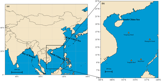
This study focuses on the SCS region (Figure 1). As one of the largest marginal seas in the western Pacific, the SCS lies in tropical–subtropical waters and exhibits a typical vertical structure characterized by high-temperature surface water and low-temperature deep water. The persistently high sea surface temperature and the widespread deep-sea basins that provide a stable supply of cold deep water offer the fundamental thermodynamic conditions for OTEC development [29].
Figure 1.
Study area and selected island and reef sites: (a) location of the South China Sea in the western Pacific; (b) locations of Yongxing Island, Huangyan Island, Yongshu Reef, and Meiji Reef.
In terms of spatial configuration, the SCS contains both vast deep-water basins and numerous isolated islands and reefs. In island and reef settings, OTEC resource characteristics are influenced by the regional background thermodynamic structure and large-scale circulation. Island and reef topography, mixing processes and nearshore dynamics may also affect these characteristics. It is therefore useful to compare the large and small windows within a unified framework. Accordingly, this study constructs a dual-scale spatial description framework centered on typical island and reef sites:
- (1)
- Large window: a domain extending ±2° in both latitude and longitude from the center of each island or reef, used to characterize the broader thermodynamic background of the surrounding waters;
- (2)
- Small window: a domain extending ±0.5° in both latitude and longitude from the center of the target site, used to characterize site-centered ΔT variations relative to the large window.
The small window still covers an area on the order of 100 km and should therefore be interpreted only as a smaller site-centered averaging domain relative to the large window, rather than as an individual reef or seawater-intake-scale domain.
2.1.1. Background Temperature Field of the South China Sea
To provide the overall thermodynamic background for the study area, temperature data for the SCS region (5° N–25° N, 105° E–120° E; Figure 1) are selected and their spatial distribution is descriptively analyzed. This domain covers the main deep-water basins and continental slope of the SCS. Shallow-water grid cells are subsequently excluded using the bathymetric mask described in Section 2.2.2, because a water depth of approximately 1000 m is generally required to obtain a stable cold water source [30,31]. Against this background, spatial averaging is used to reduce the smaller-scale variability represented in the reanalysis data and to provide a large-window reference state for comparison with the site-centered small-window results.
2.1.2. Selection of Typical Island and Reef Sites
To systematically analyze spatial differences in OTEC resources under different marine environmental conditions, four representative island and reef sites in the SCS are selected as study objects: Yongshu Reef, Meiji Reef, Yongxing Island and Huangyan Island (Figure 1). The site-center coordinates used for data extraction are Yongshu Reef (9.6° N, 113.0° E), Meiji Reef (9.9° N, 115.5° E), Yongxing Island (16.8° N, 112.3° E), and Huangyan Island (15.1° N, 117.8° E). These sites differ significantly in geographical location, bathymetric conditions and marine dynamic environment, and can represent different types of marine environments in the SCS. Among them, Yongxing Island, as the main island of the Xisha Islands, has been relatively systematically assessed for OTEC resources in its surrounding waters in a previous study [32], providing a comparable reference for the present work.
- Deep-basin setting (Yongshu Reef and Meiji Reef): located in the deep-water basin region of the south-central SCS, with large water depths in adjacent waters.
- Shelf-transitional setting (Yongxing Island): located in the Xisha Islands near the transition from relatively shallow surrounding waters to the deep-sea basin.
- Open-ocean setting (Huangyan Island): located in the open waters of the northeastern SCS, with a geographical setting distinct from the deep-basin and shelf-transition sites.
By selecting typical island and reef sites with different environmental characteristics, the ΔT resource characteristics and stability differences can be compared within a unified analysis framework.
2.2. CMEMS Reanalysis Data
2.2.1. Data Product Description
This study uses the global reanalysis dataset GLOBAL_MULTIYEAR_PHY_001_030 provided by the Copernicus Marine Environment Monitoring Service (CMEMS) [33]. This product integrates multiple satellite observations and in situ data through data assimilation techniques, providing a long-term, globally consistent time series of ocean physical parameters. The dataset has a horizontal spatial resolution of 0.083° × 0.083° and includes multiple standard depth levels in the vertical, enabling a good representation of the vertical thermal structure of the ocean. At this resolution, however, the product does not resolve individual reef structures, nearshore circulation, or seawater-intake-scale conditions. The data are accessible at https://marine.copernicus.eu/resources (accessed on 23 July 2026).
Monthly eastward and northward surface-current components (uo and vo) and mixed-layer depth (MLD) from the same CMEMS physical reanalysis product were additionally used for the process-proxy analysis. These variables were extracted for January 2010–December 2023 within the ±0.5° small windows around the four sites. Surface temperature was taken from the shallowest model layer, and deep temperature was taken from the model level nearest to 1000 m, corresponding to 902.34 m in the downloaded product.
2.2.2. Data Preprocessing Methods
Monthly mean potential temperature (thetao) data covering the SCS region (5° N–25° N, 105° E–120° E) for the period from January 2010 to December 2023 (a total of 14 years) are selected. This period was selected to maintain temporal consistency between the CMEMS reanalysis and the quality-controlled Argo observations used for validation. The resulting statistics therefore characterize the 2010–2023 study period rather than a 30-year climatological standard normal or multidecadal climate trend. The sea surface temperature is taken from the model layer closest to the sea surface, and the deep-water temperature is taken from the model layer closest to 1000 m depth. To meet the requirement of OTEC systems for a stable deep cold-water source (typically at a water depth of around 1000 m), a land–shallow-water mask is constructed based on the ETOPO1 global bathymetric model, flagging grid cells where the water depth is significantly less than 1000 m as invalid. This mask is applied to the temperature fields to eliminate the influence of shallow-water areas on the analysis. This bathymetric screening ensures that the nominal 1000 m temperature layer is available within the analyzed grid cells, but it does not constitute an engineering assessment of cold-water pipeline feasibility. After spatial screening, the monthly mean temperature difference ΔT = Ts − Td is calculated at each valid grid cell, generating a 168-month (2010–2023) time series of the ΔT field. All data processing was implemented in Python 3.9.21, primarily using xarray and NumPy.
To provide a screening-scale assessment of deep-water accessibility, local ETOPO1 bathymetry was further extracted within the ±0.5° small window around each site. The 200, 500, and 1000 m isobaths were identified, and bathymetric profiles were extracted from each nominal site center along eight fixed directions at 45° intervals. The presence of ETOPO1-resolved shallow-water grid cells within 10 km of each site center was also examined. Where both shallow-water cells and the 1000 m isobath were resolved, their minimum grid-scale horizontal separation was calculated. This analysis characterizes bathymetric accessibility only and does not represent an optimized cold-water pipeline route or establish engineering feasibility.
2.3. Argo Profile Data
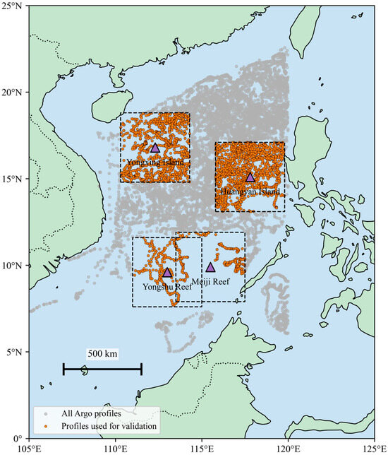
To assess the reliability of the CMEMS ocean reanalysis data in representing the vertical temperature structure in the SCS, in situ profile observations provided by the global Argo float network are introduced as an independent validation reference [23]. These data are used for subsequent comparison with the reanalysis product, providing an observation-constrained basis. The Argo profile data are obtained from the Global Argo Data Assembly Center (GDAC, IFREMER), and delayed-mode temperature profiles are selected. These data have undergone complete quality control and post hoc consistency corrections and possess a high level of credibility in climate and ocean reanalysis validation studies [34]. Considering the uneven distribution of Argo floats in the SCS and the limited number of profiles within the small window at some island and reef sites (e.g., Meiji Reef and Yongxing Island), a spatial neighborhood is used for validation to improve sample coverage and statistical stability. For validation only, valid Argo profiles are selected within a ±2° range around each site. To maintain temporal consistency with the CMEMS reanalysis data, Argo profiles from January 2010 to December 2023 are selected. The data are acquired in NetCDF format and read and preprocessed using the Python environment. Only observations with temperature and pressure quality flags set to “Good” are retained to ensure the objectivity and reliability of the validation results [35]. The spatial distribution of the filtered Argo temperature profiles is shown in Figure 2.
Figure 2.
Spatial distribution of Argo temperature profiles in the South China Sea during the 2010–2023 study period. The dashed boxes indicate the ±2° validation domains centered on the four representative sites.
3. Methods
3.1. Definition of Key Parameters for OTEC
OTEC exploits the temperature difference between warm surface seawater and cold deep seawater as its thermodynamic driving force. In this study, the ocean temperature difference is defined as:
where Ts and Td denote the monthly mean surface and deep-water temperatures, respectively, and ΔT denotes the monthly mean surface–deep temperature difference. These temperatures are calculated as spatial averages over analysis windows centered on each island or reef. For the large window, averages are calculated within a ±2° domain, whereas for the small window, they are calculated within a ±0.5° domain.
Previous studies commonly use a ΔT of approximately 20 °C as a basic thermal-resource screening criterion for OTEC [36,37]. However, preliminary analysis indicates that most islands and reefs in the SCS satisfy this condition for the majority of the study period, making the conventional threshold insufficient for distinguishing differences in resource quality and thermal-resource stability among sites. In addition, previous studies have suggested that an increase of approximately 2 °C above the baseline threshold can improve thermodynamic performance and net power generation efficiency [38].
Accordingly, this study adopts a dual-threshold framework. The criterion ΔT ≥ 20 °C is used for basic thermal-resource screening, while ΔT ≥ 22 °C is introduced as a preferred-resource threshold to enhance discrimination among islands and reefs. Subsequent analyses of resource stability and monthly low-ΔT persistence mainly use the 22 °C threshold. To assess the sensitivity of the results to threshold selection, ΔTcrit values from 18 to 23 °C were tested. Because no or only negligible low-ΔT occurrence was identified at 18 and 19 °C, the graphical comparison focuses on the more discriminative range of 20–23 °C.
3.2. Multi-Scale Analysis Framework
To compare broader background conditions with site-centered smaller-window characteristics around islands and reefs, a two-window assessment framework is established, consisting of a large window and a small window. The large window represents the broader thermodynamic background of the surrounding sea area, whereas the small window provides a smaller site-centered spatial average relative to the large window. Comparing the two windows enables quantification of window-dependent differences in OTEC resource assessment.
3.2.1. Large-Window Assessment
A large analysis window extending ±2° around each target island or reef is defined. Within this domain, valid grid cells with sufficient water depth to include the nominal 1000 m temperature layer are selected. Monthly mean surface and deep temperatures are spatially averaged to calculate the large-window temperature difference:
where Ts,L(t), Td,L(t), and ΔTL(t) denote the monthly mean surface temperature, deep-water temperature, and temperature difference for the large window at month t, respectively.
This spatial averaging reduces the smaller-scale variability represented in the reanalysis data and provides a broader thermal reference for the surrounding sea area.
3.2.2. Small-Window Assessment
A small analysis window extending ±0.5° around each island or reef is further defined. Using the same depth-selection criteria, monthly mean surface and deep temperatures are spatially averaged to calculate the small-window temperature difference:
where Ts,S(t), Td,S(t) and ΔTS(t) denote the monthly mean surface temperature, deep-water temperature, and temperature difference for the small window at month t, respectively.
Compared with single-grid extraction, this method reduces sensitivity to individual grid cells while retaining the smaller-window spatial variability represented in the reanalysis data.
3.2.3. Scale Deviation
To quantify the difference between the small- and large-window estimates, the monthly window deviation is defined as:
where ΔTS(t) and ΔTL(t) denote the small- and large-window temperature differences at month t, respectively, and ΔTdev(t) denotes their monthly difference.
The multi-year mean scale deviation is then calculated as:
where denotes the mean window deviation over the study period.
This indicator describes whether the small-window ΔT estimate is higher or lower than the corresponding large-window estimate and identifies differences that may be smoothed by broader spatial averaging.
3.3. Comprehensive Evaluation Indicators for OTEC Resources
To comprehensively characterize OTEC thermal-resource conditions and their screening implications, a multi-indicator evaluation framework is established. The selected indicators describe three aspects: thermal intensity, temporal stability, and monthly low-ΔT occurrence and persistence.
3.3.1. Multi-Year Mean Temperature Difference
The multi-year mean temperature difference during the study period is defined as:
where NM is the total number of months within the study period.
3.3.2. Minimum Temperature Difference
The minimum temperature difference during the study period is defined as:
This indicator represents the lowest monthly thermal-resource condition during the study period.
3.3.3. Coefficient of Variation
The coefficient of variation (CV) is used to quantify temporal variability:
where and denote the sample mean and sample standard deviation of the monthly ΔT series, respectively. This indicator reflects the relative temporal variability of the ΔT. A smaller CV indicates lower relative variability and greater thermal-resource stability during the study period.
3.3.4. Frequency of Low-ΔT Months
At the monthly time scale, when the monthly mean ΔT falls below the selected thermal-resource threshold ΔTcrit, that month is defined as a low-ΔT month, i.e.,:
where refers to the temperature-difference threshold.
The occurrence frequency is calculated as:
where is the number of low-ΔT months. This indicator represents the proportion of months during which the monthly mean ΔT is below the selected threshold.
3.3.5. Persistence Indicators for Consecutive Low-ΔT Months
Continuous low-ΔT months are grouped into low-ΔT periods with lengths di (unit: months). Based on these periods, two persistence indicators are defined.
- (1)
- Mean length of consecutive low-ΔT periods
where N is the total number of continuous low-ΔT segments.
- (2)
- Maximum length of consecutive low-ΔT periods
This indicator characterizes the maximum number of consecutive low-ΔT months during the study period.
3.3.6. Monthly Low-ΔT Persistence Index
To quantify the combined effect of occurrence frequency of low-ΔT months and the length of consecutive low-ΔT periods, a monthly low-ΔT persistence index is defined as:
This indicator is used for relative comparison of monthly low-ΔT persistence among different sites and averaging windows. When no low-ΔT month occurs under a selected threshold, no consecutive low-ΔT period is identified, and R is assigned a value of zero for comparative purposes.
Here f is the frequency of low-ΔT months, dmean is the mean length of consecutive low-ΔT periods, and R is the monthly low-ΔT persistence index. A higher R indicates that low-ΔT months occur more frequently and form longer consecutive periods. The index is intended only for relative monthly scale resource comparison and does not represent the probability or duration of an actual plant outage.
3.4. Validation Method Based on Argo Data
Argo delayed-mode profile data are used as independent observations to evaluate the reliability of CMEMS reanalysis data in representing vertical thermal structures in the SCS.
3.4.1. Spatiotemporal Matching and Parameter Extraction
For each quality-controlled Argo profile, the corresponding spatiotemporal position in the CMEMS reanalysis dataset is determined based on its precise observation time and location. In the temporal dimension, each Argo profile is matched to the CMEMS monthly field corresponding to its observation month. In the spatial dimension, the nearest-neighbor matching method is used to determine the corresponding grid cell, thereby constructing one-to-one sample pairs of observation and reanalysis data.
3.4.2. Extraction of Temperature Difference Parameters
Based on the matched data, the parameters required for ΔT calculation are extracted separately:
- Argo-observed ΔT: For each Argo profile, temperatures representing the surface layer (0–10 m) and the 1000 m depth are extracted by linear interpolation where necessary, and the observed temperature difference, denoted as , is calculated.
- CMEMS reanalysis ΔT: For the matched CMEMS grid cell, the monthly mean surface and deep-water temperatures are directly extracted, and the reanalysis ΔT, denoted as , is calculated.
By processing all Argo profiles that satisfy the quality control and matching conditions, a validation set containing N paired observations , is ultimately constructed, where N is the total number of successfully matched profiles.
3.4.3. Error Evaluation Indicators and Visualization
Using the paired validation set described above, this study employs multiple statistical indicators to evaluate the agreement between the CMEMS reanalysis and Argo observations [39,40]:
- (1)
- Mean Bias Error (MBE):
- (2)
- Mean Absolute Error (MAE):
- (3)
- Root Mean Square Error (RMSE):
- (4)
- Pearson Correlation Coefficient:
In addition, a scatter plot of versus is generated with a 1:1 reference line (y = x) to visualize data agreement, error dispersion, and any potential systematic bias.
3.5. Simplified Thermodynamic Sensitivity Analysis
To illustrate the relative influence of monthly thermal fluctuations and parasitic consumption on net energy generation, a simplified normalized thermodynamic model was applied. The ideal upper-bound efficiency proxy for month t was calculated as
A common reference thermal condition of Ts,ref = 28.06 °C and ΔTref = 22 °C was adopted. The corresponding reference efficiency proxy and normalized gross-power proxy were defined as
Assuming that gross-power potential varies proportionally with the ideal-efficiency proxy and that parasitic consumption is a fixed fraction λ of the reference gross-power level, the normalized net-power proxy was calculated as
The mean normalized net-energy proxy during the study period was calculated as
Parasitic-load fractions of λ = 0.20, 0.30, and 0.40 were examined, and was also evaluated for the month containing ΔTmin at each site and averaging window. These dimensionless proxies are used only to illustrate relative thermodynamic sensitivity and do not represent plant-specific power or energy production.
3.6. Proxy-Based Statistical Attribution of Small-Window ΔT Variability
For each site and month, the spatial sample standard deviation of ΔT within the ±0.5° small window was calculated as
where n is the number of valid ocean grid cells and j denotes an individual grid cell. Eddy kinetic energy was used as a proxy for mesoscale activity:
where u′ and v′ are surface-current anomalies relative to their corresponding 2010–2023 calendar-month means. The small-window mean MLD was used as a proxy for upper-ocean mixing intensity.
To reduce covariance associated with the common seasonal cycle, the corresponding calendar-month means were removed from σΔT, EKE, and MLD. The resulting anomaly series were standardized, and a multiple linear regression was fitted separately for each site:
The independent statistical association of each proxy was quantified using its standardized coefficient and incremental explained variance:
Statistical significance was evaluated using heteroskedasticity- and autocorrelation-consistent standard errors with a maximum lag of 12 months. This analysis quantifies proxy-based statistical associations rather than direct causal contributions of individual eddies or turbulent mixing.
4. Results and Discussion
4.1. Validation of CMEMS Reanalysis Data Against Argo Observations
To evaluate the reliability of the CMEMS ocean reanalysis data in representing the vertical seawater temperature structure and surface–deep temperature difference in the SCS, the reanalysis results were validated against Argo in situ profile observations at the four representative island and reef sites. The validation was conducted through spatiotemporal and depth matching to ensure physical consistency between the observational and reanalysis datasets.
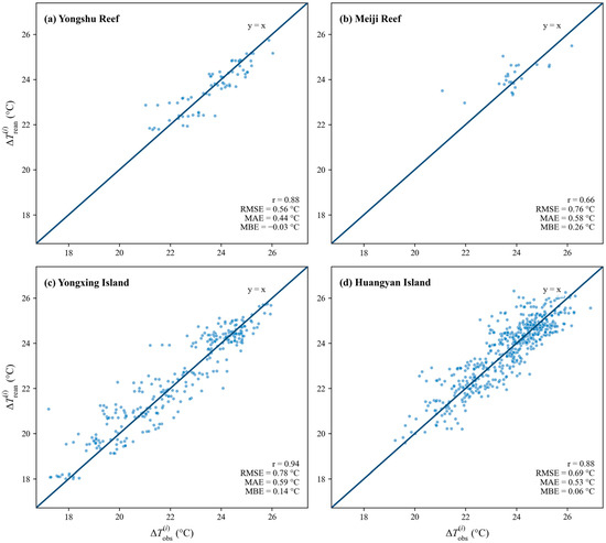
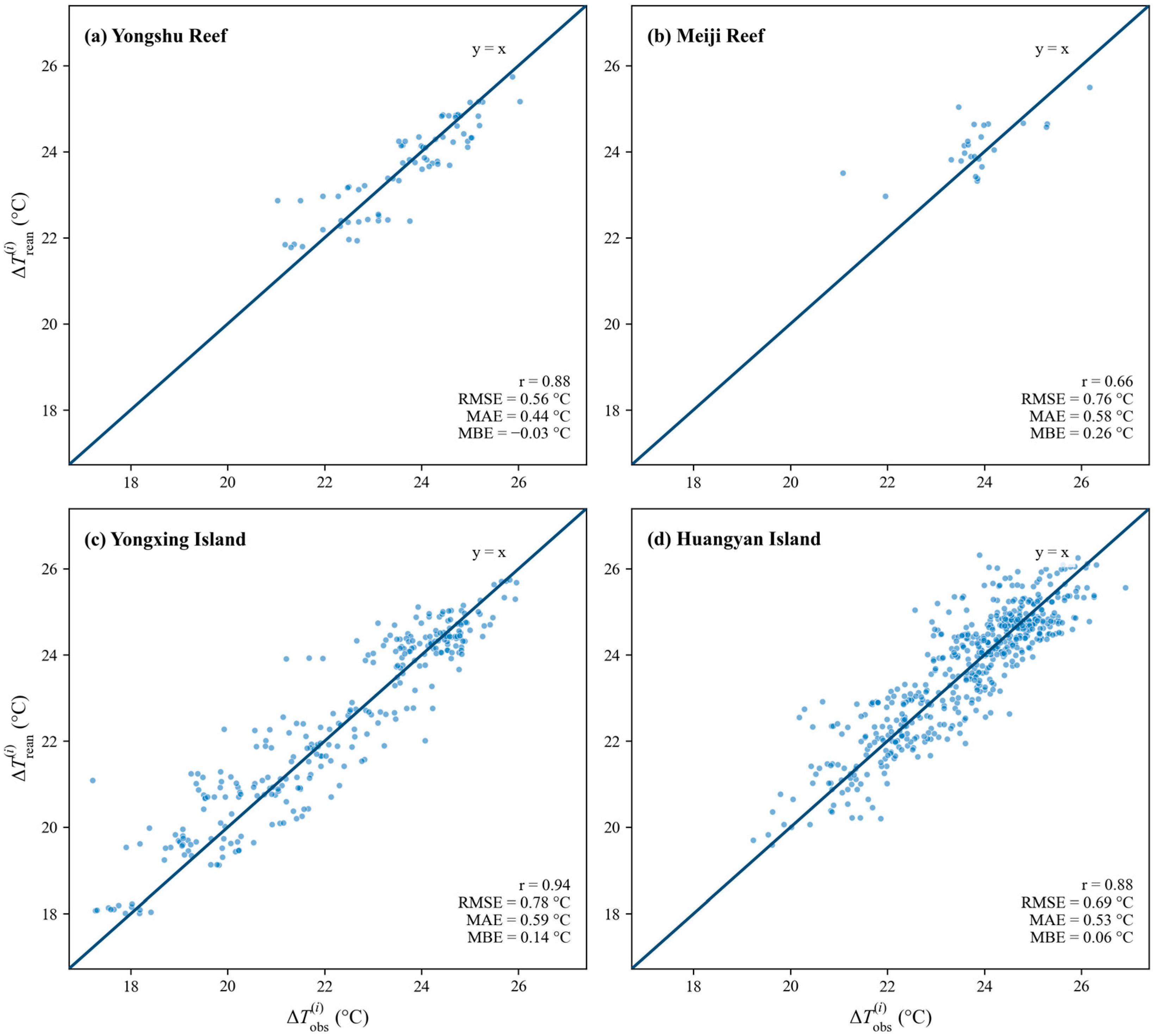
As shown in Figure 3, the CMEMS-reanalyzed ΔT values are generally distributed close to the 1:1 reference line, indicating that the reanalysis data can reasonably reproduce the main ΔT characteristics observed by Argo profiles. Quantitative validation further reveals site-dependent differences. Yongshu Reef exhibits the smallest systematic bias, with an MBE of −0.03 °C and an RMSE of 0.56 °C, indicating close agreement between the two datasets. Yongxing Island shows the highest correlation coefficient (r = 0.94), indicating that CMEMS effectively captures the observed temporal variation in ΔT at this site. Huangyan Island also shows stable validation performance, with r = 0.88 and an MAE of 0.53 °C. In comparison, Meiji Reef exhibits a relatively lower correlation coefficient (r = 0.66), although the systematic error remains moderate, with an MBE of 0.26 °C. This lower correlation may reflect spatial variability that is not fully represented by the monthly reanalysis data, although the validation comparison alone does not identify the underlying processes responsible for this discrepancy.
Figure 3.
Scatter plots comparing Argo-observed and CMEMS reanalysis ΔT at (a) Yongshu Reef, (b) Meiji Reef, (c) Yongxing Island, and (d) Huangyan Island.
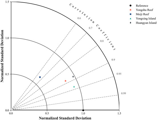
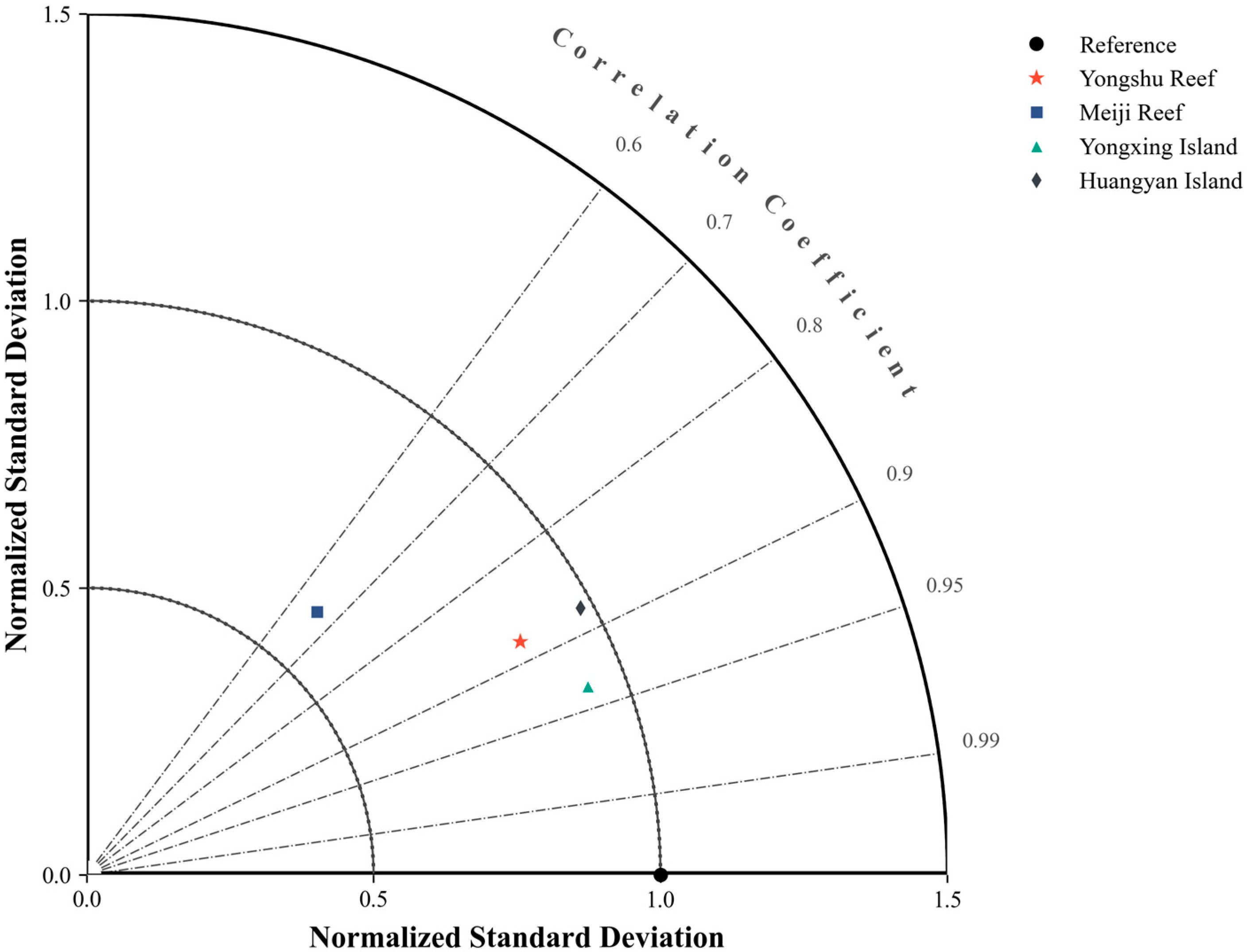
The Taylor diagram in Figure 4 further evaluates the correlation coefficient, normalized standard deviation, and centered root-mean-square difference in ΔT at each site. The normalized standard deviations of all sites fall within the range of 0.5–1.0 and are generally lower than those of the observations. This indicates that the CMEMS reanalysis data can reproduce the mean ΔT state relatively well but tend to smooth part of the observed variability. This smoothing effect is most evident at Meiji Reef, although its underlying causes cannot be inferred from the validation comparison alone. In contrast, Yongxing Island is closest to the observational reference point in the Taylor diagram, confirming its best overall agreement with Argo observations.
Figure 4.
Taylor diagram of CMEMS reanalysis ΔT relative to Argo-observed ΔT.
Overall, the CMEMS reanalysis data provide a reasonable basis for assessing the multi-year ΔT structure and its main temporal variability in the SCS during the 2010–2023 study period. However, the validation also indicates that part of the observed variability may be underestimated. Therefore, CMEMS data are suitable for broad-area and multi-year OTEC thermal-resource assessment, while the site-centered small-window analysis provides additional information on lower-tail ΔT conditions and monthly low-ΔT persistence.
4.2. Regional Thermal-Resource Background of the South China Sea
Based on the validation results, the SCS-wide thermal-resource background was further characterized to provide a broad reference for preliminary OTEC resource screening.
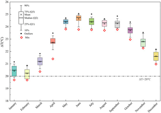
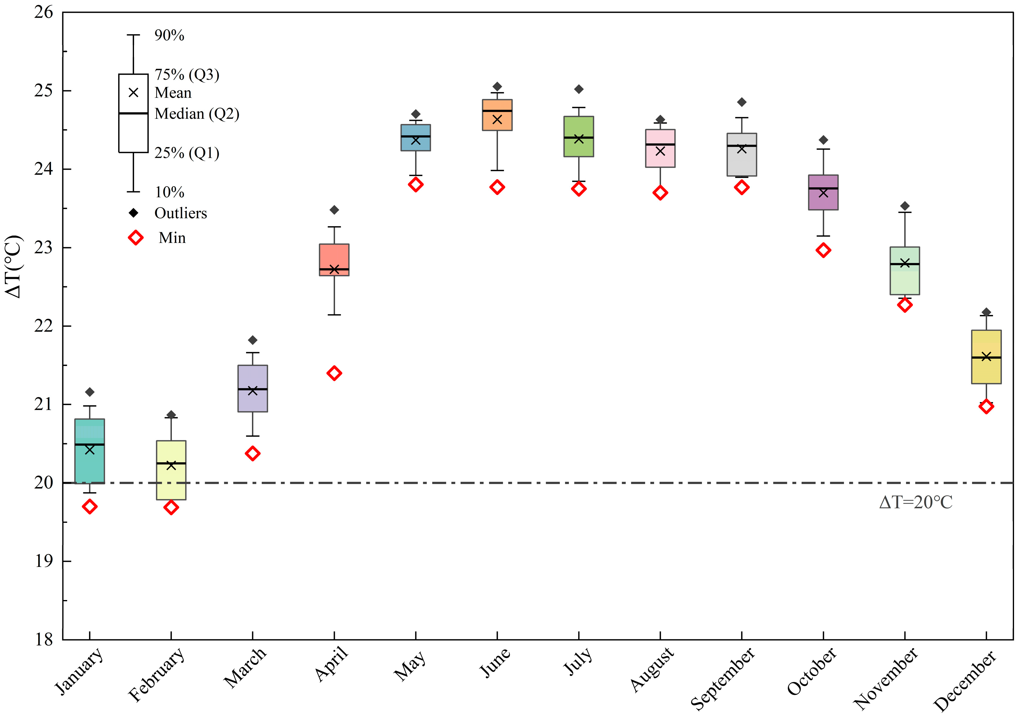
As shown in Figure 5, the SCS-wide monthly ΔT remains generally above the commonly used basic thermal-resource screening threshold of approximately 20 °C during most months. The median values show relatively stable seasonal behavior, indicating favorable multi-year thermal-resource conditions during the study period. This resource advantage is associated with the persistent tropical ocean stratification in the SCS, where warm surface seawater coexists with relatively stable deep cold water.
Figure 5.
Monthly distribution of the SCS-wide ΔT during 2010–2023 relative to the 20 °C basic thermal-resource screening threshold; the boxplot symbols are defined in the inset legend.
Nevertheless, clear seasonal variability can still be observed. During winter, particularly in January and February, the lower quartile (Q1) and minimum (Min) values decrease, and monthly low-ΔT conditions occur more frequently. These monthly low-ΔT conditions are important for thermal-resource assessment because threshold-sensitive resource characteristics cannot be fully represented by annual mean ΔT alone.
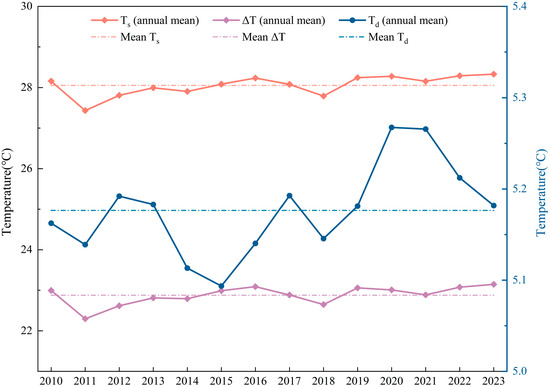
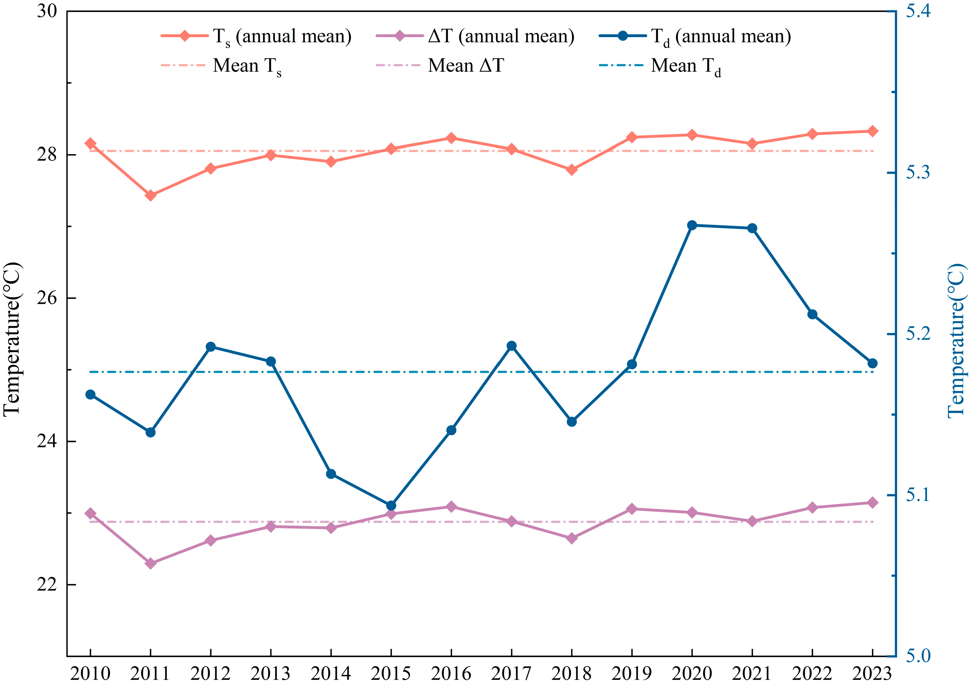
On the interannual scale (Figure 6), the annual mean Ts, Td, and ΔT values fluctuate slightly around their respective 2010–2023 study-period means of 28.06, 5.18, and 22.88 °C. No obvious directional change or abrupt shift in ΔT is observed during 2010–2023, indicating relatively stable conditions within the selected study period. This result describes variability within the 2010–2023 study period and should not be interpreted as evidence of multidecadal climatic stability. However, annual aggregation can obscure monthly low-ΔT conditions and their persistence, which are not represented by annual mean ΔT alone.
Figure 6.
Interannual variability in the SCS-wide annual Ts, Td, and ΔT during the 2010–2023; the dash-dotted lines indicate their respective study-period means.
In summary, the SCS exhibits favorable multi-year thermal-resource conditions during the 2010–2023 study period. However, monthly low-ΔT conditions remain non-negligible, especially during winter. SCS-wide statistics are useful for identifying broad resource potential but are insufficient for characterizing site-dependent lower-tail conditions and monthly low-ΔT persistence. Therefore, site-centered small-window analysis provides additional information on spatial differences in thermal-resource variability among the selected sites.
4.3. Window-Dependent Variations in ΔT Characteristics at Representative Sites
After establishing the SCS-wide thermal background, the influence of averaging-window size on ΔT characteristics was further examined at the four representative island and reef sites. The analysis focused on differences between the large- and small-window results, especially in the lower tail of the ΔT distributions, which is relevant to threshold-sensitive thermal-resource assessment.
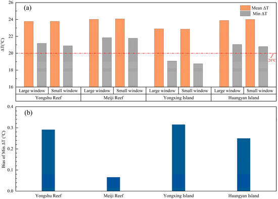
As shown in Figure 7, the multi-year mean temperature difference (ΔTmean ) remains highly consistent between the large and small windows at all sites. This indicates that averaging-window size has limited influence on the representation of the mean thermal-resource level. In contrast, the minimum temperature difference (ΔTmin) shows modest inter-window differences. In most cases, the large-window ΔTmin values are higher than corresponding small-window values, indicating that broader spatial averaging tends to smooth the lower tail of the ΔT distribution.
Figure 7.
Comparison of ΔT characteristics between the two averaging windows: (a) multi-year mean and minimum ΔT; (b) large-window minus small-window difference in minimum ΔT.
The observed inter-window differences in ΔTmin are smaller than the site-specific CMEMS–Argo validation errors reported in Section 4.1. Therefore, these differences should be interpreted as directional evidence of the spatial-averaging effect rather than as precise engineering-scale gains or losses.
Compared with the 20 °C basic thermal-resource screening threshold, Yongxing Island remains below the threshold in both windows, with the small-window result showing a further reduction in ΔTmin. For the other sites, ΔTmin remains above the threshold, but the small-window values are consistently closer to the threshold. Therefore, window-dependent differences are concentrated mainly in threshold-sensitive lower-bound conditions rather than in mean thermal-resource levels.
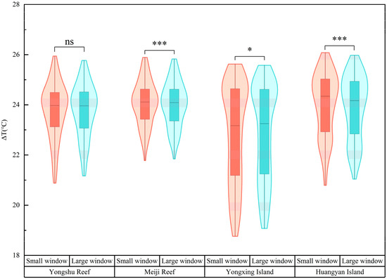
Differences between the two averaging windows are more evident in the temporal statistical distributions shown in Figure 8. For all sites, the distribution centers represented by the median values remain similar between the two windows, confirming that averaging-window size has limited influence on typical thermal conditions. However, differences appear in the lower-tail portions of the distributions. Meiji Reef shows nearly identical large- and small-window distributions, indicating weak scale sensitivity. In contrast, Yongxing Island and Huangyan Island exhibit a more extended lower tail in the small-window distributions, indicating greater sensitivity of their lower-tail estimates to averaging-window size.
Figure 8.
Temporal ΔT distributions under the small and large averaging windows at the four sites. “ns” indicates no statistically significant difference; * and *** indicate p < 0.05 and p < 0.001, respectively.
These results indicate that the primary effect of spatial averaging is not to substantially alter the mean or median ΔT, but to modify the lower-tail structure associated with threshold-sensitive thermal-resource conditions. The large window tends to smooth low-ΔT values in the distributions. However, the present analysis provides only proxy-based statistical associations and does not directly partition the inter-window differences into causal contributions from mesoscale circulation, upper-ocean mixing, short-term air–sea interactions, and other processes.
The proxy-based statistical attribution results are summarized in Supplementary Table S3. After removal of the mean seasonal cycle, EKE showed significant positive associations with small-window σΔT at Yongshu Reef, Meiji Reef, and Yongxing Island, with standardized coefficients of 0.159, 0.247, and 0.137, respectively (p < 0.05). The corresponding association at Huangyan Island was weak and not statistically significant.
MLD showed a significant negative association with σΔT only at Meiji Reef ( = −0.210, p = 0.040); the associations at the other sites were not statistically significant. The incremental explained variance associated with EKE ranged from 0.24% to 6.02%, whereas that associated with MLD ranged from 0.23% to 4.36%. The full model showed the highest adjusted R2 at Meiji Reef (0.108), while the explanatory power at the other sites was limited. These results indicate weak and site-dependent statistical associations of mesoscale activity and upper-ocean mixing with local ΔT heterogeneity, with substantial variability remaining unexplained.
Overall, changing the averaging-window size has limited influence on mean or median ΔT but modifies the representation of lower-tail conditions. For preliminary thermal-resource screening, the large-window results are suitable for representing broader multi-year mean conditions, whereas the small-window results provide additional information on site-centered lower-tail conditions. Neither window should be interpreted as representing seawater-intake-scale engineering conditions.
4.4. Monthly Low-ΔT Occurrence and Persistence Characteristics
To quantify the combined frequency and persistence of monthly low-ΔT conditions, the composite monthly low-ΔT persistence index, R = f × dmean, is used. This indicator characterizes the relative persistence of unfavorable monthly thermal-resource conditions rather than isolated low-ΔT months. A higher R indicates that low-ΔT months occur more frequently and form longer consecutive periods. It does not represent the probability or duration of an actual plant outage.
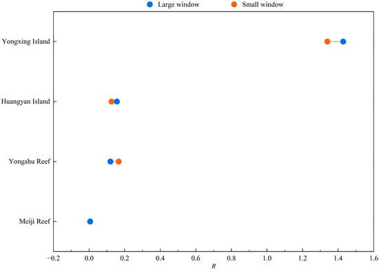
As shown in Figure 9, the monthly low-ΔT persistence index differs among the four representative sites. Yongxing Island consistently shows the highest index value in both windows, indicating relatively frequent and persistent monthly low-ΔT conditions. In contrast, Meiji Reef maintains consistently low index values, suggesting that monthly ΔT generally remains above the selected threshold. Yongshu Reef and Huangyan Island occupy intermediate positions, but their responses to averaging-window size differ, indicating site-dependent window sensitivity of monthly low-ΔT persistence.
Figure 9.
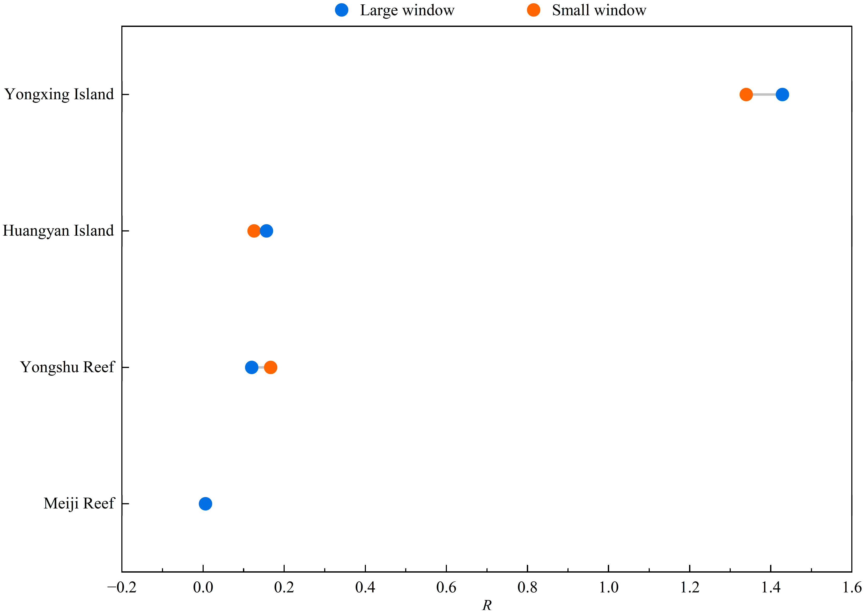
Monthly low-ΔT persistence index (R) under the large and small averaging windows at the four sites.
The influence of spatial averaging on monthly scale low-ΔT persistence is site-dependent. At Yongshu Reef, the large-window index is lower than the small-window index, indicating that broader averaging reduces the calculated frequency and/or persistence of low-ΔT months at this site. In contrast, Huangyan Island and Yongxing Island show slightly higher large-window index values. These results demonstrate that the direction and magnitude of window dependence differ among sites.However, they do not by themselves identify the spatial organization or underlying dynamic causes of the low-ΔT conditions.
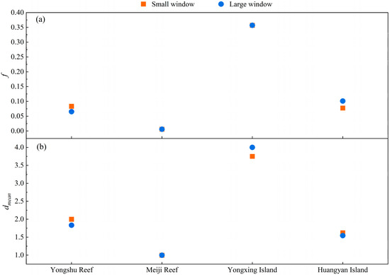
To examine the contributions of the two components to differences in R, Figure 10 presents the frequency of low-ΔT months (f) and the mean length of consecutive low-ΔT periods (dmean). Yongxing Island is characterized by both a high occurrence frequency and a long mean period length, indicating that low-ΔT months occur frequently and form relatively long consecutive periods. Yongshu Reef exhibits a moderate occurrence frequency, while its R value is also influenced by the mean length of consecutive low-ΔT periods. Huangyan Island is characterized more strongly by the frequency of low-ΔT months. In contrast, Meiji Reef maintains low values for both indicators, corresponding to relatively stable monthly thermal-resource conditions.
Figure 10.
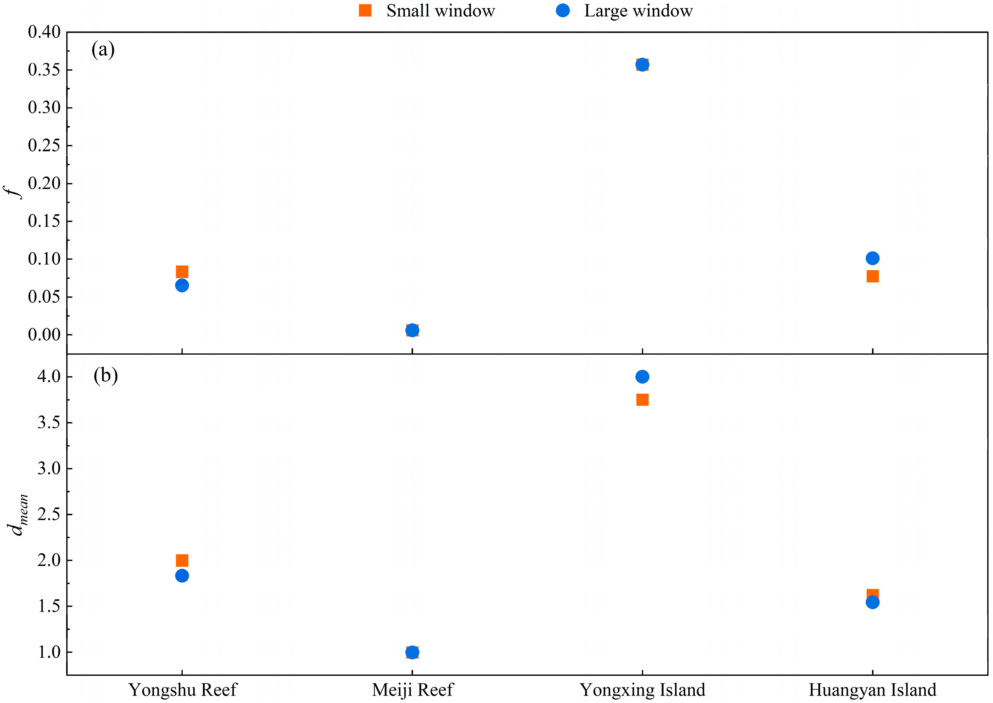
Components of the monthly low-ΔT persistence index (R): (a) frequency of low-ΔT months (f); (b) mean length of consecutive low-ΔT periods (dmean).
The maximum length of consecutive low-ΔT periods (dmax ) shows relatively limited consistency with the composite monthly low-ΔT persistence index across sites. This indicates that R reflects the combined frequency and mean period length more directly than a single maximum period.
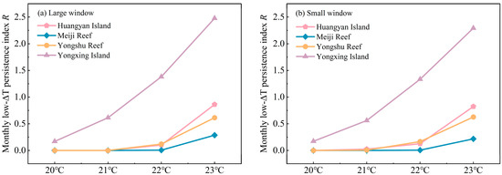
To assess the sensitivity of the monthly low-ΔT persistence index to threshold selection, ΔTcrit values from 18 to 23 °C were examined. At the 18 and 19 °C thresholds, no or only negligible low-ΔT occurrence was identified, resulting in R values of zero or close to zero and providing little discrimination among the sites. Therefore, Figure 11 focuses on the more informative range of 20–23 °C.
Figure 11.
Sensitivity of the monthly low-ΔT persistence index (R) to thresholds from 20 to 23 °C for (a) the large window and (b) the small window.
As shown in Figure 11, R generally increases as the threshold rises from 20 to 23 °C, although the magnitude of increase differs among sites. Yongxing Island consistently exhibits the highest R values in both windows, with a marked increase at the 22 and 23 °C thresholds. Meiji Reef maintains the lowest values across the tested thresholds, whereas Yongshu Reef and Huangyan Island show intermediate values. Although the absolute magnitude of RRR is sensitive to threshold selection, the broad inter-site pattern remains generally consistent. These results support the use of 20 °C as a basic thermal-resource screening threshold and 22 °C as a preferred-resource threshold, while the 23 °C result provides a supplementary assessment under a stricter resource criterion. None of these thresholds should be interpreted as a universal operational cutoff.
Overall, the monthly low-ΔT persistence index is jointly determined by the frequency of low-ΔT months and the mean length of consecutive low-ΔT periods. The relative contributions of these two components differ among sites, and changing the averaging-window size can increase or decrease the calculated index depending on the site. Threshold selection affects the absolute magnitude of R, but the broad inter-site pattern remains generally consistent. These findings indicate that preliminary OTEC thermal-resource screening should consider both lower-tail conditions and monthly low-ΔT persistence rather than relying only on large-window mean conditions.
4.5. Monthly Thermal-Resource State Classification and Margin–Persistence Characteristics
Based on the window-dependent ΔT characteristics and monthly low-ΔT persistence analysis, this section further evaluates the distribution of threshold-sensitive thermal-resource conditions. A time-fraction-based monthly state classification and a margin–persistence framework are used for this purpose.
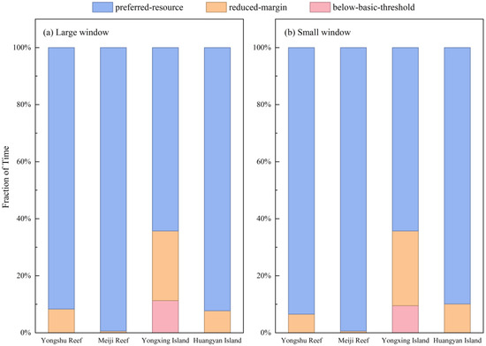
Using the two thresholds of 20 °C and 22 °C, s monthly ΔT conditions are classified into three categories: below-basic-threshold (ΔT < 20 °C), reduced-margin (20 °C ≤ ΔT < 22 °C), and preferred-resource (ΔT ≥ 22 °C). The temporal proportions of these states are shown in Figure 12. The results indicate that most sites remain at or above the basic thermal-resource screening threshold during most months of the study period. However, reduced-margin states occupy a non-negligible proportion, showing that monthly ΔT frequently lies between the basic and preferred-resource thresholds. This pattern is most evident at Yongxing Island, where transitions among the three monthly thermal-resource states occur more frequently, indicating greater threshold sensitivity.
Figure 12.
Temporal proportion of the three monthly thermal-resource states at the four sites: (a) large-window results; (b) small-window results.
Spatial averaging alters the representation of monthly thermal-resource states. The large window tends to smooth lower-tail ΔT values, which can reduce the apparent proportion of below-basic-threshold states and increase the proportion of reduced-margin states. This change reflects a redistribution among threshold-based categories caused by spatial averaging rather than an actual improvement in site conditions.
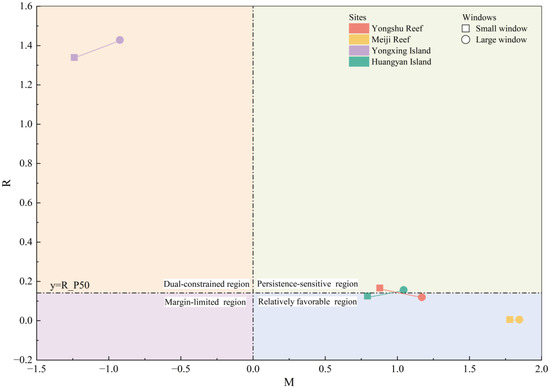
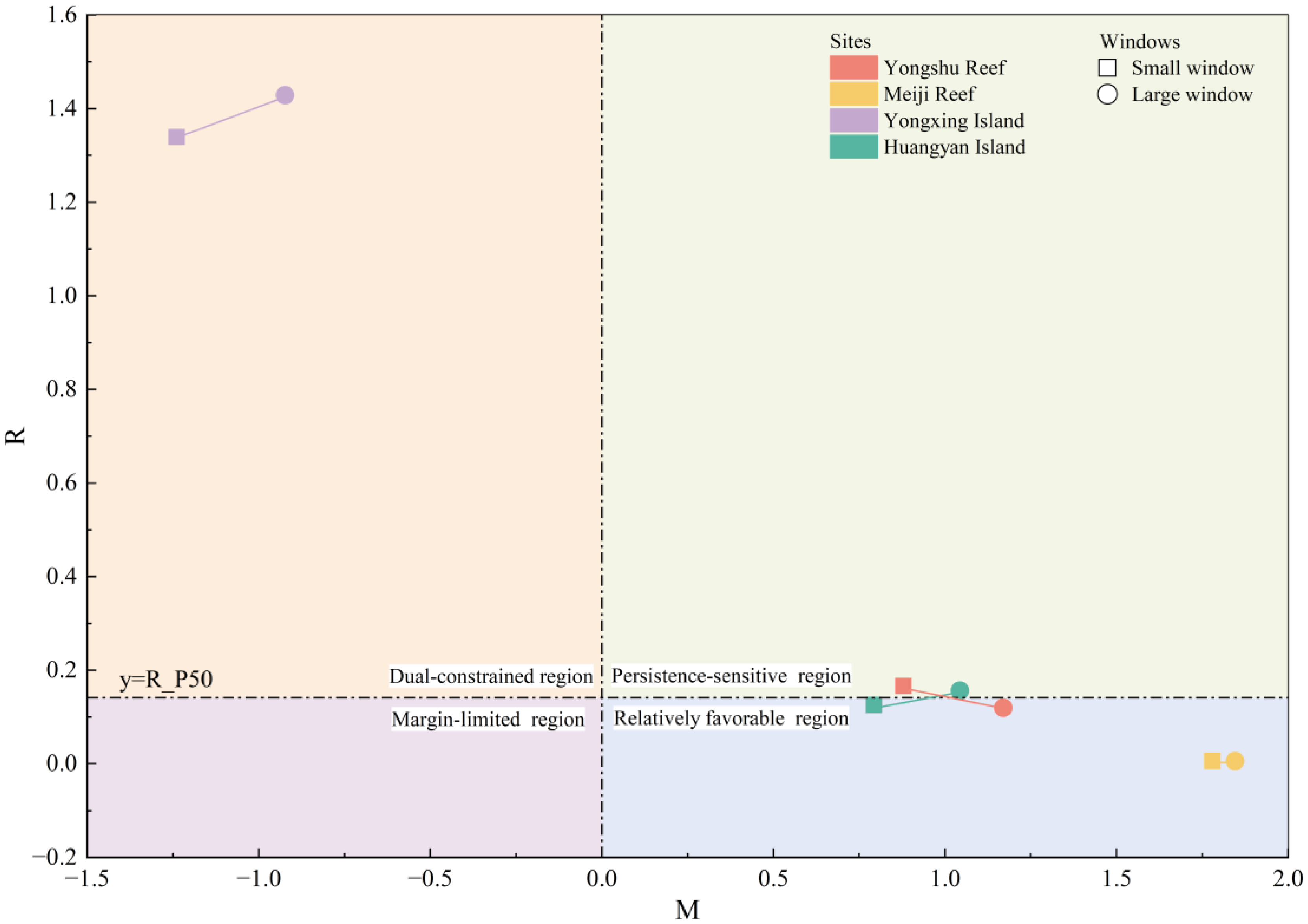
To further relate the lower thermal boundary to monthly low-ΔT persistence, the thermal-resource margin (M = ΔTmin − 20 °C) and persistence index (R) are used to construct a margin–persistence diagram (Figure 13). Sites with positive M and low R have a greater thermal-resource margin and lower monthly low-ΔT persistence, whereas sites with small M and elevated R lie closer to the basic threshold and experience more persistent monthly low-ΔT conditions. A negative M indicates that the minimum monthly ΔT during the study period falls below the 20 °C basic thermal-resource screening threshold.
Figure 13.
Thermal-resource margin–persistence space under the large and small averaging windows. Colors denote sites and symbols denote windows.
The positions of the selected sites in the M − R framework reveal distinct thermal-resource characteristics. Meiji Reef is located in the high-margin and low-persistence region, indicating a relatively favorable combination of thermal-resource margin and monthly stability. Yongxing Island occupies the negative-margin and high-persistence region, indicating the least favorable combination among the four sites. Yongshu Reef and Huangyan Island fall between these two end-members, while the relative contributions of low-ΔT frequency and mean consecutive-period length differ as discussed in Section 4.4.
The simplified thermodynamic sensitivity results are presented in Supplementary Figure S3 and Table S2. The normalized net-power proxy increases monotonically with ΔT, whereas a higher assumed parasitic-load fraction shifts the proxy to lower values. Under the common reference surface temperature of 28.06 °C, the values at ΔT = 20 °C are 0.709, 0.609, and 0.509 for λ = 0.20, 0.30, and 0.40, respectively. At the preferred-resource threshold of ΔT = 22 °C, the corresponding values are 0.800, 0.700, and 0.600. Site- and window-specific values for the months containing ΔTmin together with the study-period mean , are summarized in Supplementary Table S2. These results illustrate that lower-tail ΔT conditions reduce the relative thermodynamic driving force and increase the importance of parasitic consumption in net-generation assessment. The proxies are dimensionless sensitivity indicators rather than predictions of plant-specific net power.
Overall, monthly thermal-resource conditions are jointly characterized by the minimum thermal boundary and monthly low-ΔT persistence. The thermal-resource margin indicates whether the minimum monthly ΔT during the study period remains above the 20 °C basic screening threshold, whereas R describes the combined frequency and mean consecutive-period length of low-ΔT months. Therefore, preliminary thermal-resource screening should jointly consider ΔTmin, monthly low-ΔT persistence, and averaging-window dependence.
4.6. Comprehensive Evaluation and Relative Site Ranking for Preliminary OTEC Thermal-Resource Screening
To compare the relative thermal-resource suitability of the four representative island and reef sites, a comprehensive evaluation method was developed based on ΔT characteristics and monthly low-ΔT persistence. Three indicators were selected: multi-year mean temperature difference (ΔTmean), minimum temperature difference (ΔTmin), and monthly low-ΔT persistence index (R). These indicators represent the multi-year thermal-resource level, the lower thermal boundary, and monthly low-ΔT persistence, respectively.
For the positive indicators (ΔTmean and ΔTmin):
For the negative indicator (R):
Min–max normalization was performed separately within each averaging window using the four selected sites. Therefore, the normalized values support relative comparison among sites within the same window, and their absolute magnitudes should not be directly compared between the large and small windows.
On this basis, a composite scoring model was constructed:
The weighting reflects the relative emphasis placed on each indicator in the preliminary thermal-resource screening. The lower thermal boundary represented by ΔTmin is assigned the highest weight (w2 = 0.4), while ΔTmean and R, representing the multi-year resource level and monthly low-ΔT persistence, respectively, are assigned equal weights (w1 = w3 = 0.3).
Because these weights are judgment-based, the robustness of the site ranking was further examined using five weighting schemes: the baseline scheme, an equal-weight scheme, and three alternative schemes emphasizing ΔTmean, ΔTmin, and R, respectively.
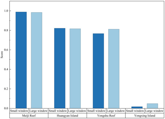
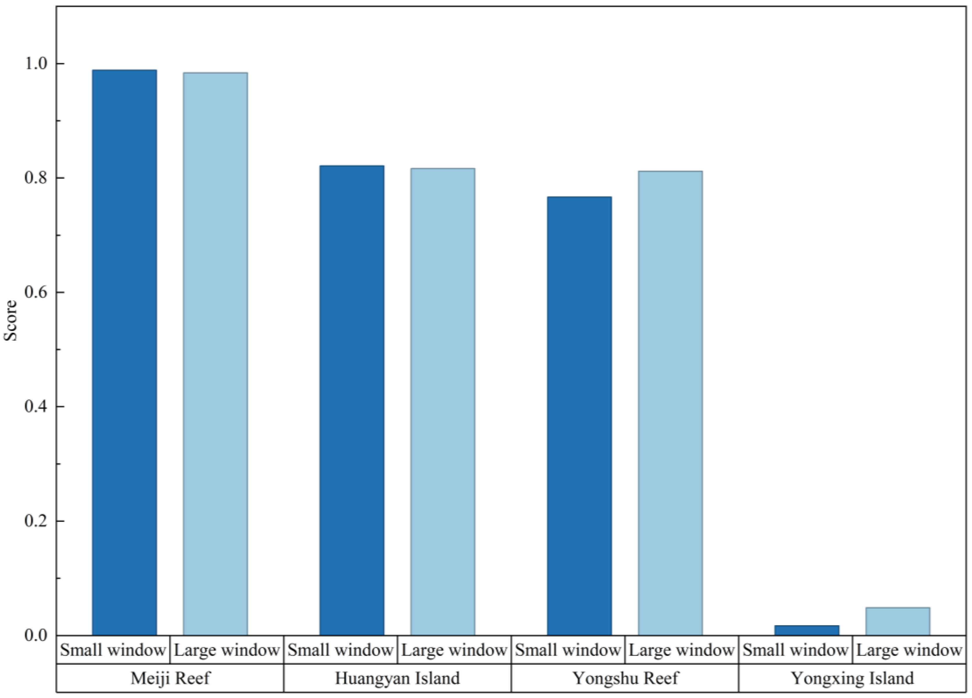
The composite evaluation results under the baseline weighting scheme are shown in Figure 14. The ranking pattern remains generally consistent between the two averaging windows. Meiji Reef achieves the highest relative thermal-resource score among the four sites, followed by Huangyan Island and Yongshu Reef, whereas Yongxing Island ranks lowest. These results indicate that the relative thermal-resource score depends not only on mean ΔT but also on the lower thermal boundary and monthly low-ΔT persistence.
Figure 14.
Composite thermal-resource scores of the four sites under the large and small averaging windows using the baseline weighting scheme.
The sensitivity of the relative site ranking to indicator weights is summarized in Table 1. Across all five weighting schemes, Meiji Reef consistently ranks first and Yongxing Island ranks last in both averaging windows. The small-window ranking remains unchanged under all weighting schemes, following the order Meiji Reef > Huangyan Island > Yongshu Reef > Yongxing Island. For the large window, the same ranking is maintained under the baseline, equal-weight, mean-ΔT-emphasis, and persistence-emphasis schemes. Only when greater weight is assigned to ΔTmin do Yongshu Reef and Huangyan Island exchange positions, while the highest- and lowest-ranked sites remain unchanged. These results indicate that the overall ranking is generally robust to weight selection, although the relative positions of the two intermediate sites in the large window show some sensitivity to the emphasis placed on minimum ΔT. Therefore, the baseline ranking should be interpreted as a generally robust relative thermal-resource ordering, while the middle-ranking positions remain conditional on the weighting preference.
Table 1.
Sensitivity of relative site rankings to different indicator-weighting schemes under large and small averaging windows.
Compared with the small-window results, the large-window evaluations generally exhibit slightly higher ΔTmin values and different monthly low-ΔT persistence index values. These differences reflect the influence of spatial averaging on lower-tail conditions and consecutive low-ΔT months. Although they mainly affect indicator values rather than the broad ranking pattern, the small-window results provide complementary information on site-centered lower-tail characteristics. Neither window represents seawater-intake-scale engineering conditions.
To further synthesize the preliminary screening implications of the assessment results, Table 2 summarizes the dominant thermal characteristics, monthly low-ΔT features, window sensitivities, and relative thermal-resource implications of the four sites. The comparison highlights that relative OTEC thermal-resource suitability depends not only on the mean thermal-resource level but alsoon monthly low-ΔT persistence and averaging-window sensitivity.
Table 2.
Thermal-resource characteristics and preliminary screening implications for the four representative sites.
Overall, Meiji Reef shows the highest relative thermal-resource suitability among the four sites under the indicators and baseline weights adopted in this study, whereas Yongxing Island obtains the lowest relative score. These results confirm that mean ΔT alone is insufficient for characterizing relative OTEC thermal-resource suitability, particularly when lower-bound conditions and monthly low-ΔT persistence differ among sites.
The local ETOPO1 bathymetry and eight-direction profiles are presented in Supplementary Figures S1 and S2, and the screening results are summarized in Supplementary Table S1. The 1000 m isobath is present within the ±0.5° window around all four sites, indicating the regional availability of deep water. The minimum ETOPO1-resolved separations between shallow-water cells and the 1000 m isobath were 3.69 km for Yongshu Reef, 4.09 km for Meiji Reef, 10.82 km for Yongxing Island, and 3.69 km for Huangyan Island (Supplementary Table S1). The bathymetric profiles show clear directional differences in the shallow-to-deep transition. Yongxing Island exhibits a relatively broad and direction-dependent transition, whereas Huangyan Island reaches water depths greater than 1000 m over shorter horizontal distances in most directions. Yongshu Reef and Meiji Reef also show pronounced directional variability. These results provide screening-scale information on deep-water accessibility rather than cold-water pipeline routes or engineering feasibility.
It should be noted that the present evaluation reflects relative thermal-resource suitability among the four sites rather than the predicted performance or final siting feasibility of a specific OTEC plant. Additional factors, including seawater-intake conditions, cold-water pipe routing, seabed characteristics, pumping power, hydrodynamic and environmental constraints, system configuration, infrastructure availability, and techno-economic performance, should be incorporated in future site-specific assessments.
4.7. Research Limitations and Future Work
This study identifies window-dependent differences in OTEC thermal-resource assessment and monthly low-ΔT persistence in the SCS. However, several limitations remain.
- (1)
- The monthly CMEMS reanalysis dataset at 0.083° resolution cannot resolve individual eddies, internal waves, submesoscale processes, or turbulent mixing rates. The EKE–MLD regression provides a quantitative proxy-based assessment of their statistical associations with small-window σΔT, but it does not establish direct causal process contributions. The generally limited adjusted R2 values also indicate that other unresolved processes and data-resolution effects remain important. Higher-resolution velocity and turbulence fields, moored observations, and site-specific measurements are required for process-resolving attribution and intake-scale assessment.
- (2)
- A higher CV indicates greater relative monthly thermal-resource variability and may imply greater balancing requirements for a fixed plant and load profile. However, storage capacity cannot be derived from CV alone; it additionally requires time-resolved net-power deficits, load demand, storage efficiency, allowable depth of discharge, and reliability criteria.
- (3)
- The supplementary ETOPO1 analysis provides screening-scale information on local bathymetry and the proximity of the 1000 m isobath. However, its one-arc-minute resolution does not fully resolve narrow reef platforms, detailed seabed slopes, or candidate cold-water pipeline corridors. Therefore, the results should not be interpreted as actual pipeline lengths or engineering feasibility; site-specific design requires high-resolution multibeam bathymetry, geotechnical data, and route optimization.
- (4)
- The 2010–2023 record characterizes the selected study period rather than a 30-year climatological standard normal and may not fully capture decadal variability. Future climate extensions should bias-correct CMIP6 surface- and 1000 m-temperature projections against CMEMS over a common historical period. For climate model k and scenario s, the projected temperature difference may be calculated as , and its projected change is . The same ΔTmin, monthly low-ΔT persistence, and normalized net-power indicators could then be evaluated under scenarios such as SSP2–4.5 and SSP5–8.5 to assess long-term thermal-resource and technical resilience. A full CMIP6 ensemble analysis is beyond the historical CMEMS–Argo scope of the present study.
Overall, the two-window framework supports preliminary OTEC thermal-resource screening, but the small window should not be interpreted as an individual reef- or seawater-intake-scale engineering domain.
5. Conclusions
This study developed a two-window assessment framework to evaluate OTEC thermal resources and monthly low-ΔT persistence at four representative island and reef sites in the South China Sea. By integrating large- and small-window analyses with Argo-based validation, the window-dependent characteristics of the surface–deep temperature difference, lower-tail conditions, and monthly low-ΔT persistence were examined. The main conclusions are as follows:
- (1)
- Changing the averaging-window size primarily affects the lower-tail structure of the ΔT distributions rather than the multi-year mean thermal-resource level. The large window has limited influence on ΔTmean but tends to produce slightly higher ΔTmin values and a smoother lower tail. Because the inter-window differences in ΔTmin are smaller than the CMEMS–Argo validation errors, they should be interpreted as directional evidence of spatial-averaging effects rather than as precise engineering-scale differences.
- (2)
- Monthly low-ΔT persistence is jointly determined by the frequency of low-ΔT months and the mean length of consecutive low-ΔT periods. The threshold-sensitivity analysis shows that R is zero or close to zero at 18 and 19 °C and generally increases as the threshold rises from 20 to 23 °C, while the broad inter-site pattern remains consistent. These results support the use of 20 °C as a basic thermal-resource screening threshold and 22 °C as a preferred-resource threshold rather than universal operational cutoffs.
- (3)
- The four representative sites exhibit distinct monthly low-ΔT persistence characteristics. Yongxing Island has the highest frequency and longest consecutive low-ΔT periods, resulting in the highest persistence index. Meiji Reef maintains relatively high and stable ΔT conditions and the lowest persistence index. Yongshu Reef and Huangyan Island occupy intermediate positions, although the relative contributions of low-ΔT-month frequency and consecutive-period length differ between the two sites.
- (4)
- Mean ΔT alone is insufficient for relative OTEC thermal-resource assessment. The proposed framework combines the multi-year resource level, minimum thermal boundary, and monthly low-ΔT persistence. Under the baseline weights, Meiji Reef has the highest relative thermal-resource suitability among the four sites, whereas Yongxing Island has the lowest relative score. The weight-sensitivity analysis shows that the highest- and lowest-ranked sites remain unchanged under all five weighting schemes, while the relative positions of Yongshu Reef and Huangyan Island change only when greater emphasis is placed on ΔTmin in the large window.
Overall, preliminary OTEC thermal-resource screening in island and reef environments should combine large-window mean conditions with small-window information on lower-tail ΔT, ΔTmin, and monthly low-ΔT persistence. Neither window represents individual reef- or seawater-intake-scale engineering conditions. Final OTEC siting and design therefore require additional assessment of bathymetry, cold-water pipe routing, pumping power, hydrodynamic and environmental conditions, infrastructure, and techno-economic performance.
Supplementary Materials
The following supporting information can be downloaded at https://www.mdpi.com/article/10.3390/jmse14151396/s1.
Author Contributions
Conceptualization, B.D. and Y.C.; methodology, B.D.; software, B.D.; validation, B.D.; formal analysis, B.D.; investigation, B.D.; data curation, B.D.; writing—original draft preparation, B.D.; writing—review and editing, B.D. and Y.C.; visualization, B.D.; supervision, Y.C.; project administration, Y.C.; funding acquisition, Y.C. All authors have read and agreed to the published version of the manuscript.
Funding
This research was funded by the National Natural Science Foundation of China, grant number 52206246; the Natural Science Foundation of Hebei Province, grant number E2023502104; and the Fundamental Research Funds for the Central Universities, grant number 2024MS144.
Institutional Review Board Statement
Not applicable.
Informed Consent Statement
Not applicable.
Data Availability Statement
The CMEMS reanalysis data used in this study are publicly available from the Copernicus Marine Service. Argo profile data are publicly available from the Global Data Assembly Centre, and ETOPO1 bathymetric data are publicly available from NOAA. The processed data and Python scripts supporting the findings of this study are available from the corresponding author upon reasonable request.
Conflicts of Interest
The authors declare no conflicts of interest.
Nomenclature
| Symbols | |
| di | length of the ith consecutive low-ΔT period [months] |
| dmax | maximum length of consecutive low-ΔT periods [months] |
| dmean | mean length of consecutive low-ΔT periods [months] |
| mean normalized net-energy proxy | |
| G | normalized gross-power proxy |
| M | Thermal-resource margin [°C] |
| NM | total number of months within the study period |
| the number of months in which low-ΔT events occur | |
| normalized net-power proxy | |
| R | the monthly low-ΔT persistence index |
| Td | monthly deep seawater temperature [°C] |
| small-window deep-water temperature [°C] | |
| large-window deep-water temperature [°C] | |
| Ts | monthly surface seawater temperature [°C] |
| small-window mean surface temperature [°C] | |
| large-window mean surface temperature [°C] | |
| incremental variance explained by EKE | |
| incremental variance explained by MLD | |
| the temporal mean of all monthly ΔT [°C] | |
| the selected thermal-resource threshold [°C] | |
| the deviation of monthly basis [°C] | |
| the multi-year mean of the deviation [°C] | |
| small-window monthly ΔT [°C] | |
| the multi-year mean ΔT [°C] | |
| minimum ΔT [°C] | |
| the observed ΔT [°C] | |
| the reanalysis ΔT [°C] | |
| large-window monthly ΔT [°C] | |
| small-window spatial sample standard deviation of ΔT | |
| standardized regression coefficient for EKE | |
| standardized regression coefficient for MLD | |
| the mean value of ΔT | |
| standard deviation of ΔT | |
| ideal upper-bound efficiency proxy | |
| reference ideal-efficiency proxy | |
| λ | assumed parasitic-load fraction relative to the reference gross-power level |
| Abbreviations | |
| CV | Coefficient of Variation |
| EKE | Eddy Kinetic Energy proxy |
| MAE | Mean Absolute Error |
| MBE | Mean Bias Error |
| MLD | Mixed-Layer Depth |
| OTEC | Ocean Thermal Energy Conversion |
| RMSE | Root Mean Square Error |
| SCS | South China Sea |
References
- Chen, Y.; Dai, B.; Ren, W.; Niu, H.; Chen, Z. A Comprehensive Review of Energy Security in Islanded Regions: Challenges, Strategies, and Sustainable Development Pathways. Renew. Sustain. Energy Rev. 2025, 220, 115879. [Google Scholar] [CrossRef] [Scilit]
- Jithendranath, J.; Das, D.; Guerrero, J.M. Probabilistic Optimal Power Flow in Islanded Microgrids with Load, Wind and Solar Uncertainties Including Intermittent Generation Spatial Correlation. Energy 2021, 222, 119847. [Google Scholar] [CrossRef] [Scilit]
- Roy, D.; Taghavifar, H.; Shivaprasad, K.V.; Wang, Y.; Das, B.K.; Roskilly, A.P. Multi-Criteria Decision-Making and Uncertainty Analyses of off-Grid Hybrid Renewable Energy Systems for an Island Community. Energy Convers. Manag. 2025, 343, 120120. [Google Scholar] [CrossRef] [Scilit]
- Vicente, M.; Imperadore, A.; Correia Da Fonseca, F.X.; Vieira, M.; Cândido, J. Enhancing Islanded Power Systems: Microgrid Modeling and Evaluating System Benefits of Ocean Renewable Energy Integration. Energies 2023, 16, 7517. [Google Scholar] [CrossRef] [Scilit]
- Rojas-Jerez, J.F.; T., L.T.V.; López-Castrillón, W.; Sanabria-Sanabria, J.E.; A., E.F.N.; A., A.D.P. Employing the Ocean Thermal Gradient for Green Hydrogen Production: An Analysis of Closed- and Open-Cycle Ocean Thermal Energy Conversion in the Colombian Caribbean Sea. Energy Convers. Manag. 2026, 350, 120980. [Google Scholar] [CrossRef] [Scilit]
- Faizatama, A.M.; Firdaus, N.; Adiputra, R.; Prabowo, A.R.; Ghanbari-Ghazijahani, T.; Fazeres-Ferradosa, T.; Melnyk, O.; Salamena, G.G. Hydrodynamic Impact of Cold-Water Pipes and Mooring Systems on KVLCC2 for Floating OTEC Platforms. Ocean Eng. 2025, 341, 122491. [Google Scholar] [CrossRef] [Scilit]
- Adiputra, R.; Rasgianti; Nugraha, A.D.; Puryantini, N.; Salamena, G.G.; Prabowo, A.R. Comprehensive Assessment of Working Fluid Selection for Ocean Thermal Energy Conversion. Results Eng. 2025, 28, 108086. [Google Scholar] [CrossRef] [Scilit]
- Guo, H.; Liu, M.; Xiao, L.; Jia, Z.; Li, J. Review of Fluid Mechanics Problems on Ocean Thermal Energy Conversion (OTEC) Pipeline Systems. Sustain. Energy Technol. Assess. 2025, 83, 104569. [Google Scholar] [CrossRef] [Scilit]
- Feng, X.; He, G.; Ma, Q.; Li, J.; Wu, Z.; Lu, H.; Wang, C.; Wang, S. Design Optimization and Similarity Analysis of Non-Azeotropic Organic Radial Inflow Turbine for OTEC Power and Water Cogeneration. Appl. Therm. Eng. 2025, 270, 126176. [Google Scholar] [CrossRef] [Scilit]
- Taroual, K.; Nachtane, M.; Adeli, K.; Boulzehar, A.; Saifaoui, D.; Faik, A. Marine Renewable Energy for Hydrogen Production: Advancing towards a Sustainable Future through Technological, Economic, and Environmental Frontiers– a Review. Renew. Sustain. Energy Rev. 2026, 226, 116304. [Google Scholar] [CrossRef] [Scilit]
- Hall, K.; Kelly, S.; Henry, L. Site Selection of Ocean Thermal Energy Conversion (OTEC) Plants for Barbados. Renew. Energy 2022, 201, 60–69. [Google Scholar] [CrossRef] [Scilit]
- Li, D.; Fan, C.; Zhang, C.; Chen, Y. Control Strategy of Load Following for Ocean Thermal Energy Conversion. Renew. Energy 2022, 193, 595–607. [Google Scholar] [CrossRef] [Scilit]
- Lutfi, Y.M.; Adiputra, R.; Prabowo, A.R.; Utsunomiya, T.; Erwandi, E.; Muhayat, N. Assessment of the Stiffened Panel Performance in the OTEC Seawater Tank Design: Parametric Study and Sensitivity Analysis. Theor. Appl. Mech. Lett. 2023, 13, 100452. [Google Scholar] [CrossRef] [Scilit]
- Saadha, A.; Ishihara, K.N.; Ogawa, T.; Okumura, H. Climate-Driven Resource, Cost and Resilience Assessment of Ocean Thermal Energy Conversion Systems. Energy Convers. Manag. 2026, 347, 120599. [Google Scholar] [CrossRef] [Scilit]
- Saadha, A.; Ishihara, K.N.; Ogawa, T.; Okumura, H. Optimizing Energy Futures in the Maldives: A Study of Ocean Thermal Energy Conversion Technology Energy Mixes. Renew. Energy 2026, 256, 124204. [Google Scholar] [CrossRef] [Scilit]
- Herrera, J.; Sierra, S.; Hernández-Hamón, H.; Ardila, N.; Franco-Herrera, A.; Ibeas, A. Economic Viability Analysis for an OTEC Power Plant at San Andrés Island. J. Mar. Sci. Eng. 2022, 10, 713–730. [Google Scholar] [CrossRef] [Scilit]
- Ou, F.; Ning, B.; Li, J.; Tian, Y.; Qiu, D.; Geng, L.; Jin, X. Design, Construction and Sea Trials of the 20 kW Ocean Thermal Energy Conversion in the South China Sea. Energy 2026, 342, 139641. [Google Scholar] [CrossRef] [Scilit]
- Langer, J.; Infante Ferreira, C.; Quist, J. Is Bigger Always Better? Designing Economically Feasible Ocean Thermal Energy Conversion Systems Using Spatiotemporal Resource Data. Appl. Energy 2022, 309, 118414. [Google Scholar] [CrossRef] [Scilit]
- Langer, J.; Blok, K. The Global Techno-Economic Potential of Floating, Closed-Cycle Ocean Thermal Energy Conversion. J. Ocean Eng. Mar. Energy 2024, 10, 85–103. [Google Scholar] [CrossRef] [Scilit]
- Jing, F.; Wang, X.; Mei, Y.; Tian, R. A Comprehensive Review on Ocean Thermal Energy Conversion Technology: Thermodynamic Optimization, Multi-Energy Integration, and Byproduct Utilization. Energy Convers. Manag. X 2025, 27, 101188. [Google Scholar] [CrossRef] [Scilit]
- Soto Calvo, M.; Lee, H.S. Ocean Thermal Energy Conversion (OTEC) Potential in Central American and Caribbean Regions: A Multicriteria Analysis for Optimal Sites. Appl. Energy 2025, 394, 126182. [Google Scholar] [CrossRef] [Scilit]
- Majumder, M.Z.H.; Shampa, M.T.A.; Islam, M.A.; Deowan, S.A.; Hafiz, F. Marine Renewable Energy Harnessing for Sustainable Development in Bangladesh: A Technological Review. Energy Rep. 2024, 11, 1342–1362. [Google Scholar] [CrossRef] [Scilit]
- Park, K.; Yang, Z.; Copping, A.E.; Rollano, F.T. A Modeling Study of Ocean Thermal Energy Conversion Resource and Potential Environmental Effects around Kailua-Kona, Hawaii. Renew. Energy 2025, 253, 123616. [Google Scholar] [CrossRef] [Scilit]
- Tian, F.; Li, X.; Liu, M.; Xia, C.; Guo, X.; Fang, X.; Huang, L. Application of a GIS-Based Multi-Criteria Decision-Making Approach to the Siting of Ocean Thermal Energy Conversion Power Plants: A Case Study of the Xisha Sea Area, China. Energies 2024, 17, 5097. [Google Scholar] [CrossRef] [Scilit]
- Boodoo, A. Dual-Use Wave Energy Opportunities in Caribbean Small Island Developing States: A Screening Framework for Renewable Energy and Coastal Protection. Energy Sustain. Dev. 2026, 92, 101977. [Google Scholar] [CrossRef] [Scilit]
- Du, T.; Jing, Z.; Wu, L.; Wang, H.; Chen, Z.; Ma, X.; Gan, B.; Yang, H. Growth of Ocean Thermal Energy Conversion Resources under Greenhouse Warming Regulated by Oceanic Eddies. Nat. Commun. 2022, 13, 7249. [Google Scholar] [CrossRef] [Scilit] [PubMed]
- Tian, Z.; Zou, X.; Zhang, Y.; Gao, W.; Chen, W.; Peng, H. 4E Analyses and Multi-Objective Optimization for an Innovative Solar-Ocean Thermal Energy Conversion/Air Conditioning System. J. Clean. Prod. 2023, 414, 137532. [Google Scholar] [CrossRef] [Scilit]
- Tao, S.; Liu, K.; Yan, H.; Meng, M.; Huang, C.-Y.; Shen, C.-C.; Zhang, H.; Yu, K.; Shi, Q. Coral-Inferred High Seasonal Sea Surface Temperature in the South China Sea at 7.4 Thousand Years Ago. Earth Planet. Sci. Lett. 2025, 672, 119700. [Google Scholar] [CrossRef] [Scilit]
- Gao, Y.; Yu, Q.; Liu, G. Research on the Distribution Characteristics of Temperature Difference Energy and Site Selection in the South China Sea. Port Eng. Technol. 2024, 61, 145–150. [Google Scholar]
- Ding, J.; Wu, G.; Jiang, B.; Hou, E.; Bai, Y.; Wang, X. CORA Data-based Study on Space-time Characteristics of Thermal Energy in South China Sea. Acta Energiae Solaris Sin. 2023, 44, 402–409. [Google Scholar] [CrossRef]
- Wu, H.; Yang, X.; Li, Z.; Kuang, R. Benefit Analysis of Deep-sea Temperature Difference Energy Utilization Based on South China Sea. Acta Energiae Solaris Sin. 2024, 45, 536–544. [Google Scholar] [CrossRef]
- Yan, S.; Zhou, C.; Zhu, F.; Zhang, J. Evaluation of Ocean Thermal Energy Conversion (OTEC) and Site Selection Analysis of Power Station in Yongxing Island, South China Sea. Acta Energiae Solaris Sin. 2023, 44, 401–409. [Google Scholar] [CrossRef]
- Feng, B.; Ding, M.; Xie, L.; Lin, P.; Zheng, W.; Liu, H. An Assessment of Mesoscale Eddies Simulated by a Global Eddy-Resolving Ocean Forecast System in the South China Sea. Atmos. Ocean. Sci. Lett. 2026, 19, 100706. [Google Scholar] [CrossRef] [Scilit]
- Merchel, M.; Walczowski, W.; Rak, D.; Wieczorek, P. The Use of Argo Floats as Virtual Moorings for Monitoring the South Baltic Sea. Oceanologia 2024, 66, 99–110. [Google Scholar] [CrossRef] [Scilit]
- Jha, R.K.; Bhaskar, T.V.S.U. Generation and Assessment of ARGO Sea Surface Temperature Climatology for the Indian Ocean Region. Oceanologia 2023, 65, 343–357. [Google Scholar] [CrossRef] [Scilit]
- Cheddie, L.; Kelly, S.; Balladin, D. Utilizing AHP-TOPSIS to Select an OTEC Cycle Type for Tobago. Renew. Energy 2026, 257, 124727. [Google Scholar] [CrossRef] [Scilit]
- Aresti, L.; Christodoulides, P.; Michailides, C.; Onoufriou, T. Reviewing the Energy, Environment, and Economy Prospects of Ocean Thermal Energy Conversion (OTEC) Systems. Sustain. Energy Technol. Assess. 2023, 60, 103459. [Google Scholar] [CrossRef] [Scilit]
- Ticona Rollano, F.; García Medina, G.; Yang, Z.; Copping, A. Resource Assessment of Ocean Thermal Energy Conversion in Puerto Rico and U.S. Virgin Islands. Renew. Energy 2025, 246, 122907. [Google Scholar] [CrossRef] [Scilit]
- Tong, Y.; Sun, W.; Li, J.; Chen, W.; Li, Y.; Li, B.; Li, S.; Shi, P. The Climatic Mutation in the Long-Term Trends of Wind and Wave Energies in the South China Sea. Energy 2025, 340, 139206. [Google Scholar] [CrossRef] [Scilit]
- Nicolosi, C.F.; Tina, G.M. Monte Carlo and Bootstrap Approaches for Power System Adequacy: A Study on Atmospheric Variables Correlations. Int. J. Electr. Power Energy Syst. 2025, 169, 110827. [Google Scholar] [CrossRef] [Scilit]

Disclaimer/Publisher’s Note: The statements, opinions and data contained in all publications are solely those of the individual author(s) and contributor(s) and not of MDPI and/or the editor(s). MDPI and/or the editor(s) disclaim responsibility for any injury to people or property resulting from any ideas, methods, instructions or products referred to in the content. |
© 2026 by the authors. Licensee MDPI, Basel, Switzerland. This article is an open access article distributed under the terms and conditions of the Creative Commons Attribution (CC BY) license.