


Abstract
Suspended sediment in tidal flows progressively erodes composite turbine blades, with the leading edge being the most vulnerable region. While solid-particle erosion has been studied extensively for metallic components, predictive frameworks for fibre-reinforced polymers under tidal conditions remain limited. This study presents a two-dimensional computational framework that couples a Reynolds-averaged Navier–Stokes solution of the flow around a NACA 63-415 hydrofoil with Lagrangian erosion analysis (125 µm quartz particles) using the Oka erosion model previously calibrated for FR4 glass–fibre composite. Turbulent steady-state simulations were performed in STAR CCM+ (2510.0001) as the CFD software package at five angles of attack (0°, 2.5°, 5°, 7.5°, 10°) at a chord-based Reynolds number of 1.6 × 10⁶, with hydrodynamic predictions validated against published experimental lift-to-drag data. Using the relevant Oka model enabled computation of the erosion rate distribution along the blade section based on particles’ local impact velocities and angles. The resulting profiles consistently exhibit a near-zero erosion zone at the stagnation area, followed by a sharply localised peak erosion within the first 10 to 20 per cent of the chord on the upper surface. A B-spline functional representation of the chordwise erosion distribution is proposed, providing a compact and reproducible basis for subsequent roughness-based hydrodynamic analysis.
1. Introduction
Renewable energy technologies are increasingly replacing fossil fuels in the global energy portfolio in response to the climate crisis and rising carbon emissions [1,2]. Solar and wind energy systems have seen widespread deployment in recent years. Despite covering more than 70% of the Earth’s surface, oceans remain underutilised in renewable energy production, partly due to environmental and technological constraints [3]. Recent studies continue to highlight that technical reliability, environmental exposure, and long-term degradation remain key barriers to large-scale deployment of marine energy technologies [4,5,6,7,8].
Marine renewable energy sources include ocean thermal gradients, salinity differences, wave power, offshore wind, and tidal currents [9]. Among these, offshore wind and tidal energy are considered the most promising for large-scale electricity generation due to the high kinetic energy densities involved [10,11]. This study focuses on tidal energy converters.
Tidal currents arise from gravitational interactions between the Earth and orbiting celestial bodies, producing predictable bidirectional flows [12]. This predictability, rooted in astronomical tidal cycles, provides tidal energy with a key advantage over intermittent wind and solar resources [13]. Furthermore, the substantially higher density of water, approximately 850 times that of air, allows tidal turbines to produce greater thrust and power than their wind-based counterparts at similar flow velocities [14].
Tidal streams can reach velocities of up to 2.5 m/s in constricted regions near headlands and islands, making them a concentrated and valuable energy resource [15]. Various technologies have been proposed to harness this energy, including horizontal-axis turbines, vertical-axis turbines, oscillating hydrofoils, and Venturi devices [11,16]. Among these, horizontal-axis tidal turbines have emerged as the most commercially viable configuration, mirroring their dominance in the wind energy sector. These systems benefit from buoyancy-assisted design concepts that mitigate gravitational loads and enhance operational stability [17,18].
The components of tidal turbines must withstand cyclic mechanical loading, corrosion, cavitation, and erosion to maintain both structural integrity and hydrodynamic performance [19,20]. Although all of these degradation mechanisms can affect the material, structural response, and power output of the turbine, both individually and synergistically, the present study considers sediment-induced erosion in isolation, focusing on its effect on a composite blade section in seabed-mounted turbines. CFD-based erosion frameworks have been applied to natural-gas elbows [21,22], slurry pipelines and pumps [23,24], marine propellers [25], tidal turbines [26], wind turbines [27,28,29], and rain erosion studies [30]. These studies show that accurate modelling of multiphase flow and particle–wall interactions is essential for understanding material degradation patterns. Erosion-induced surface degradation is inherently time-dependent and spatially nonuniform, altering blade aero- and hydrodynamic performance [31,32,33]. The development and validation of reliable tidal turbine technologies span several decades, driven by the need for long-lasting, efficient systems capable of operating in harsh marine conditions [34]. In addition, tidal turbines are subject to torque loads estimated to be approximately 50% higher than those experienced by comparable wind turbines, necessitating robust structural designs to ensure uninterrupted operation over projected lifespans of 20 to 25 years [35].
Erosion of tidal turbine blades, particularly at the leading edge, represents a significant durability and performance challenge for marine renewable energy systems. Among the various environmental stressors affecting turbine operation, suspended particle impacts associated with sediment-laden tidal currents are a dominant driver of surface degradation over time [36]. These interactions result in gradual material loss and surface topographical changes, which can compromise structural integrity and contribute to premature failure [37,38]. CFD simulations based on Eulerian–Lagrangian approaches have demonstrated strong potential for predicting such erosion trends under complex multiphase flow conditions, particularly when combined with turbulence-resolving models and impact-driven erosion correlations [39,40].
Both flow conditions and particle dynamics govern the evolution of leading-edge erosion, and its progression is typically highly localised [41]. This localisation presents challenges for developing conventional erosion models, requiring specified information on the target material’s response to various particle impact scenarios. Recent advances in CFD, particularly the use of Eulerian–Lagrangian solvers and particle-tracking tools, have enabled more detailed predictions of erosion rates in complex geometries [42]. These methods can resolve local impact velocities, angles, and residence times, providing valuable insight into wear-prone regions even within simplified two-dimensional domains. However, interpretation of such high-resolution outputs remains challenging without a structured framework for spatial mapping and comparison, particularly when attempting to relate numerical predictions to experimental measurements or field observations.
In earlier work, Habibi et al. [43] conducted slurry-erosion tests on FR4 glass–fibre composite specimens, a material relevant to tidal turbine blade applications. Their results revealed nonlinear relationships between surface roughness evolution and erosion progression, highlighting the limitations of bulk-averaged erosion metrics. Building on these findings, the present study aims to predict and interpret localised erosion patterns on the leading edges of tidal turbine blades using a CFD-based approach calibrated against experimental data. By mapping erosion at discrete surface locations, the analysis provides physically meaningful insight into how flow conditions and particle impact dynamics govern material loss in critical blade regions.
The present study adopts a two-dimensional section-level approach, which is most representative of mid-span conditions on blades of moderate to high aspect ratio, where spanwise velocity components are relatively small and chordwise flow dominates. This approach is consistent with established practice in blade-erosion research: Vimalakanthan et al. [29] employed 2D RANS CFD to investigate leading-edge erosion on real wind turbine blade sections extracted at defined spanwise positions, demonstrating that section-level analysis provides a reliable basis for assessing erosion distribution and aerodynamic performance. Carraro et al. [31] compared two- and three-dimensional models and found that the pressure field and lift were reproduced accurately, with the main discrepancies occurring in drag. The applicability of this assumption diminishes toward the tip and root regions, where radial-flow acceleration, hub interference, and three-dimensional separation can substantially alter particle trajectories and erosion patterns. Similarly, at angles of attack (AOAs) approaching stall, three-dimensional boundary-layer effects may cause 2D predictions to diverge from the true erosion distribution. The present results should therefore be interpreted as representative of mid-span, attached-flow conditions. Extension to three-dimensional blade geometries is identified as a priority for future work.
By enabling region-specific analysis and fitted erosion profiles, the proposed segmentation and mapping approach enhances the interpretation of erosion trends, facilitates comparison across AOAs, and supports calibration of predictive erosion models. Ultimately, this methodology helps bridge the gap between detailed numerical erosion predictions and practical damage assessment in marine energy systems. In future work, these erosion maps will also support hydrodynamic performance evaluations by linking erosion-induced roughness distributions to changes in blade behaviour.
2. Methodology
The methodology adopted in this study was developed to predict and analyse the spatial distribution of erosion on a tidal turbine hydrofoil exposed to sediment-laden flow, with particular emphasis on leading-edge degradation. A validated CFD framework was coupled with a calibrated Oka erosion model to quantify erosion severity under representative operating conditions. The hydrofoil investigated was based on the NACA 63-415 profile, which is commonly used to represent tidal turbine blade sections, and simulations were conducted at multiple AOAs.
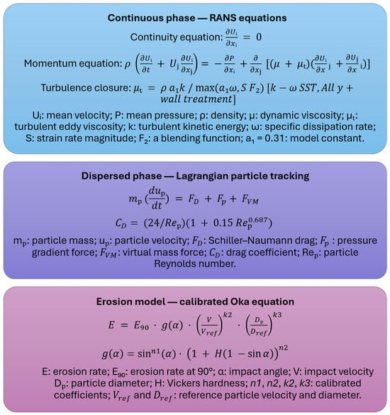
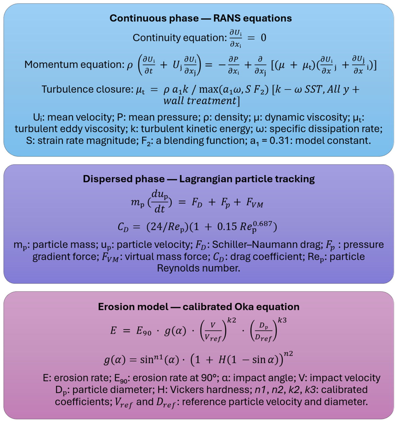
The numerical procedure began with steady-state two-dimensional Reynolds-averaged Navier–Stokes (RANS) simulations of the smooth hydrofoil, governed by the incompressible continuity and momentum equations closed with the k-ω SST turbulence model. Subsequently, Lagrangian Multiphase particle injection was introduced to model sediment transport within the flow, with particle motion governed by an equation of motion that incorporates drag, pressure gradient, and virtual mass forces. Quartz sand particles were tracked under a one-way coupling assumption, and local impact conditions were extracted directly from the resolved particle trajectories. A previously calibrated Oka erosion model for FR4 glass–fibre-reinforced composite materials was employed to compute erosion rates at discrete surface locations. The governing equations of the integrated framework are summarised in Figure 1. The statistical repeatability of the Lagrangian erosion predictions was evaluated across all five AOAs, as detailed in Section 2.3.
Figure 1.
Block diagram of the integrated CFD–Lagrangian Multiphase erosion framework, illustrating the governing equations of the continuous phase, dispersed phase, and erosion model components [44,45,46,47,48].
The key input parameters for the CFD framework, including fluid properties, particle properties, boundary conditions, and solver settings, are summarised in Table 1.
Table 1.
Summary of CFD input parameters for the integrated Lagrangian Multiphase erosion framework.
The following subsections describe the hydrofoil geometry and surface segmentation strategy, the CFD setup and validation procedure, the particle injection and tracking configuration, the calibrated erosion model formulation, and the optimisation of parcel stream counts to achieve stable and repeatable Lagrangian erosion results.
2.1. Geometry and Domain Configuration
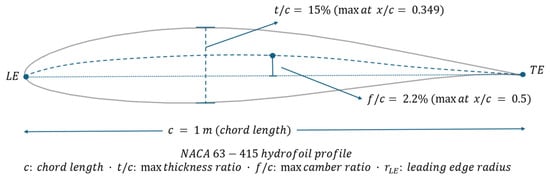
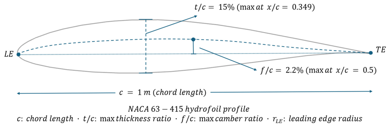
The hydrofoil examined in this study was based on the NACA 63-415 profile. The NACA 63-415 profile is characterised by a maximum relative thickness of 15% of chord, located at 34.9% of chord from the leading edge, a maximum camber of 2.2% of chord at 50% of chord [49]. These geometric parameters are illustrated in Figure 2. This section was selected for its relevance to tidal turbine blade design and for allowing direct validation of the numerical simulations against the experimental measurements reported by Bak et al. [50]. The chord length was normalised to one metre for all simulations. The flow was modelled as two-dimensional, consistent with the Reynolds number regime considered in the CFD setup.
Figure 2.
Schematic of the NACA 63-415 hydrofoil profile with key geometric parameters.
The computational domain was defined as a rectangular region extending 40 m in the streamwise direction and 15 m in the transverse direction. These dimensions were selected to ensure adequate clearance between the hydrofoil and domain boundaries, thereby minimising blockage effects and preventing artificial acceleration of the freestream flow. The hydrofoil was positioned centrally within the domain to maintain symmetric boundary influence. Details of the mesh generation procedure and local refinement strategy are provided in the following subsection.
2.2. CFD Setup and Validation
Two-dimensional steady-state simulations were performed using a RANS framework to resolve the flow around the NACA 63-415 hydrofoil at various AOAs. The flow was assumed to be incompressible, and a uniform freestream velocity was prescribed to achieve a Reynolds number of 1.6 × 10⁶, based on the chord length and fluid properties (V ≈ 1.6 m/s, ν = 10−6 m2/s). This Reynolds number is representative of full-scale operating conditions for tidal turbine blades.
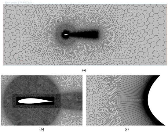
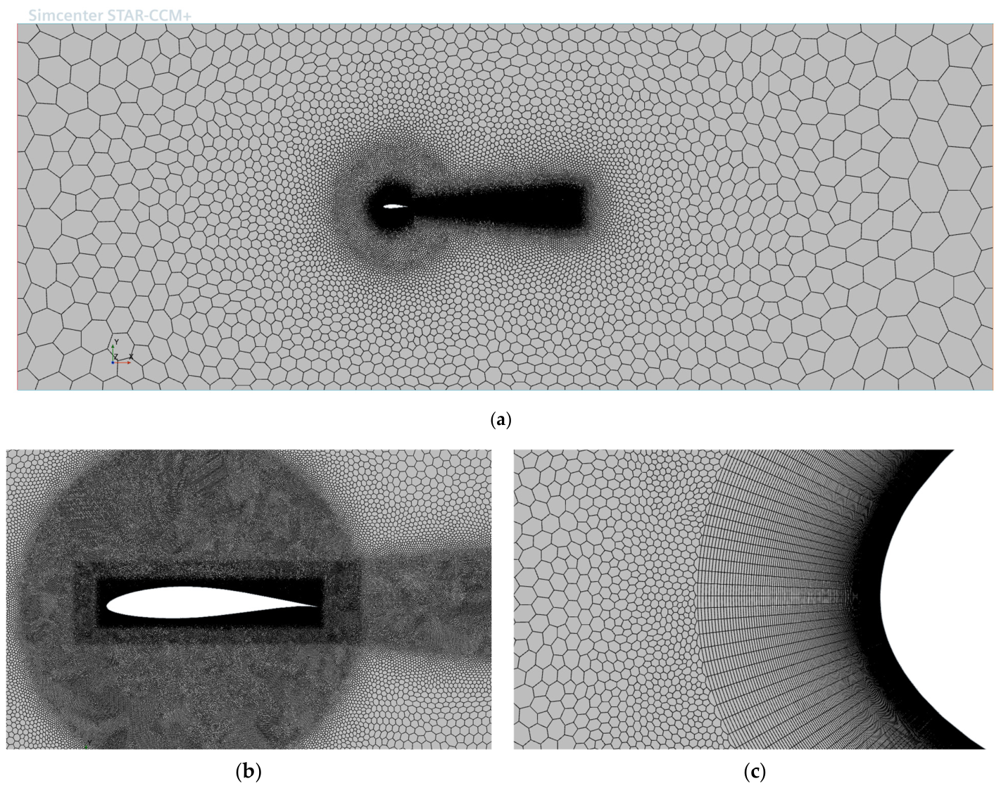
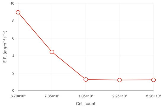
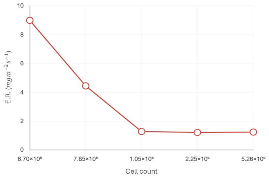
The computational domain was discretised using an unstructured mesh composed of polygonal elements in the main flow region and prism layers adjacent to the hydrofoil surface. A total of 200 prism layers were employed, with a first-layer thickness of 9.5 × 10⁶ m and an overall boundary-layer thickness of approximately 0.02 m. Local mesh refinement was applied in the leading-edge and wake regions to accurately resolve pressure gradients, flow separation, and recirculation zones. For the zero-angle-of-attack case, the resulting mesh comprised 1,046,988 cells. A representative view of the computational mesh, including refinement zones and boundary-layer structure, is shown in Figure 3. A dedicated mesh sensitivity study was carried out to determine the optimal cell count required to achieve converged Eulerian flow fields. The assessment used y+ and the target lift-to-drag coefficients (Cl/Cd) listed in Table 2. Mesh refinement was then extended further to ensure a stable Lagrangian analysis with respect to the predicted erosion rate, ER. The results of the mesh sensitivity study at an AOA of 0° are presented in Figure 4. The Eulerian solution satisfied the validation requirements with a minimum mesh size of 670,228 cells. The mesh was further refined to stabilise the Lagrangian prediction. Beyond 1,046,988 cells, the computed erosion rate changed by less than 5% and approached a plateau as the mesh was increased to 5,262,009 cells. The same mesh strategy, accounting for both Eulerian and Lagrangian requirements, was applied at the remaining angles of attack. The resulting cell counts at 2.5°, 5°, 7.5° and 10° were 1,046,988, 1,040,455, 1,035,903 and 1,035,903, respectively.
Figure 3.
Computational mesh domain (a) the overview of the boundaries; (b) local mesh refinement near the hydrofoil surface and wake region; (c) boundary-layer mesh at the leading edge, illustrating prism layers used to resolve near-wall flow with y+ < 1.
Table 2.
Validation of CFD results against experimental data for NACA 63-415 at Re = 1.6 × 10⁶.
Figure 4.
Mesh study to determine the optimal mesh cell count to capture the final erosion rate.
To accurately capture near-wall flow behaviour, the mesh was designed to maintain a non-dimensional wall distance of over the majority of the hydrofoil surface. This criterion was satisfied for all simulated cases. Figure 5 illustrates the resulting distribution for the zero-angle-of-attack condition as a representative example.
Figure 5.
Wall y+ along the simulated smooth NACA 63-415, in steady state turbulent flow, at Re = 1.6 × 10⁶.
As noted above, the k–ω Shear Stress Transport (SST) turbulence model was employed throughout the simulations due to its established capability in resolving boundary-layer flows subject to adverse pressure gradients. Its robustness and accuracy in external hydrodynamic applications make it particularly suitable for the present study, where near-wall shear stresses and potential flow separation are critical.
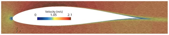
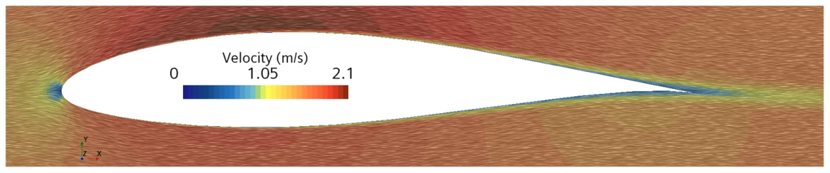
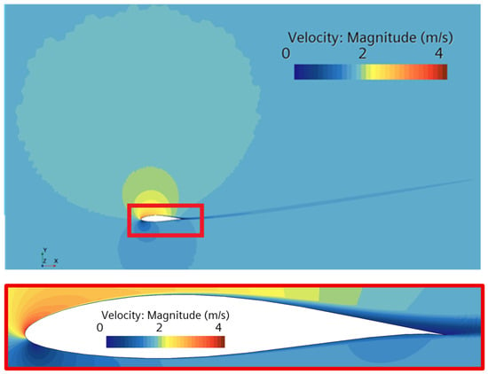
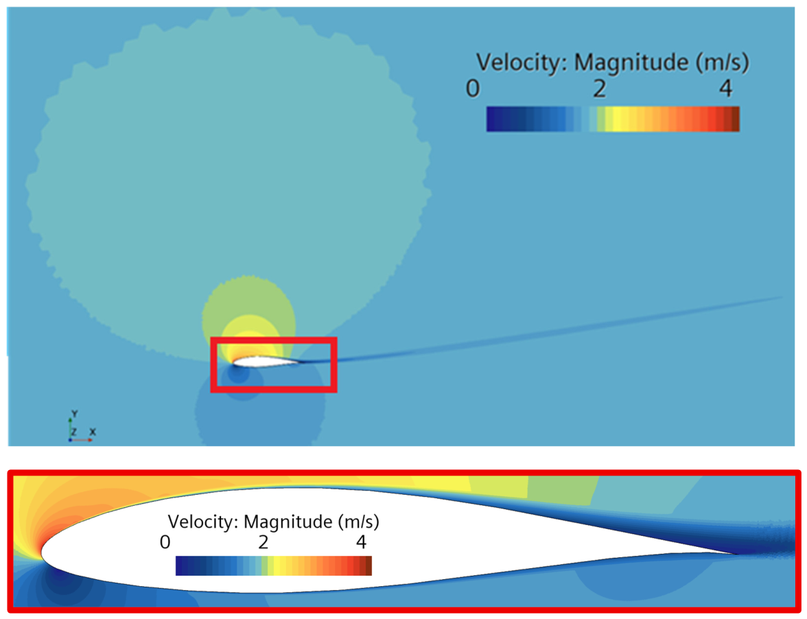
Boundary conditions were configured to represent realistic operating conditions. A uniform velocity profile with a prescribed turbulence intensity was imposed at the inlet, while a static pressure condition was applied at the outlet. The upper and lower boundaries were defined as symmetry planes, and a no-slip condition was enforced on the hydrofoil surface. A representative velocity field for the zero-angle-of-attack case is shown in Figure 6, highlighting the stagnation point, the attached boundary layer, and the downstream wake structure.
Figure 6.
Flow velocity field around NACA 63-415 at Re = 1.6 × 10⁶, and AOA = 0°.
The numerical framework was validated by comparing the computed lift-to-drag ratio () with experimental measurements reported by Bak et al. [50] for the NACA 63-415 aerofoil. Validation was performed at the same Reynolds number and under equivalent inflow conditions for a NACA 63-415 hydrofoil. As summarised in Table 2, the numerical predictions show close agreement with experimental data across the full range of AOAs considered. The lift-to-drag ratio, a key indicator of hydrodynamic efficiency, was selected as the primary validation metric. The observed consistency between numerical and experimental results confirms the suitability of the CFD framework for the erosion simulations presented in this study.
Across the five AOAs, Cl errors ranged from 0.5% to 8.2% while Cd errors ranged from 3.7% to 10.1%. Both increased progressively with AOA and reached their maximum at AOA = 10°, consistent with the known sensitivity of RANS turbulence closures to adverse pressure gradients and incipient separation at higher AOAs. A drag coefficient error of this magnitude at the highest AOA considered is consistent with commonly accepted validation standards in the CFD erosion and blade aerodynamics literature; Vimalakanthan et al. [29], for example, validated lift and drag forces for wind turbine blade leading-edge erosion studies within a 10% threshold. For erosion prediction specifically, the relevant quantity is the near-wall velocity field governing particle trajectories rather than the integrated force coefficients, which are influenced by boundary-layer development across the full chord.
2.3. Lagrangian Injection Setup
Following validation of the Eulerian flow field, the simulation framework was extended to include solid-particle tracking to model erosion behaviour. This transition to a coupled Eulerian–Lagrangian formulation enabled the resolution of individual particle trajectories, using the previously converged flow field as the carrier phase.
Sediment-laden inflow was represented by a surface injection applied along the inlet boundary using the Lagrangian Multiphase model implemented in STAR-CCM+. The injected particles were quartz sand with a density of 2650 kg m−3 and a size range of 100–150 µm. For the erosion calculations, a monodisperse particle diameter of 125 µm was adopted, corresponding to the mean of the measured size range. The use of a single representative diameter is a widely adopted simplification in CFD-based erosion modelling, particularly when the primary objective is to characterise the spatial distribution and relative trends of erosion rather than to predict absolute wear rates for a polydisperse sediment [26,40]. This assumption was supported by the independent 45° impingement case reported in the earlier calibration study [51]. A CFD simulation using 125 µm particles predicted an erosion rate of 0.0143 g/h, compared with the measured value of 0.0124 g/h obtained from a test using the actual 100–150 µm sand distribution. The corresponding error was 15.5%. This result confirms that the representative diameter produces predictions consistent with polydisperse experimental data under similar conditions. The Oka particle-size scaling term, (as explained in Section 2.4), gives factors of approximately 0.535 at 100 µm and 1.666 at 150 µm, relative to 125 µm. These values illustrate the theoretical sensitivity of the absolute erosion-rate magnitude to particle size. It is emphasised that neither extreme represents the actual sediment condition, and these bounds should be interpreted as theoretical limits rather than estimates of the practical error introduced by the monodisperse assumption. A fully polydisperse simulation is identified as a direction for future work.
Particles were released at the local freestream velocity and at a sediment concentration of 3% by mass. This concentration matched that used in the flat-plate calibration experiments and in the independent 45° validation case that underpins the calibrated Oka model. This mass concentration corresponds to a particle volume fraction of approximately 1.18 × 10⁻², calculated from the quartz sand and seawater densities and independently verified against the injector mass flow rate and geometry. A one-way coupling approach was adopted: the flow field influenced particle motion, but particle-to-fluid momentum feedback was neglected. The Eulerian flow field was first converged independently, after which the Lagrangian solver used the resulting solution as the carrier phase for particle tracking. The validity of this assumption is supported by the low particle Stokes number, approximately 0.004 based on the hydrofoil chord length, indicating that particles behave essentially as passive tracers with negligible inertial slip relative to the carrier flow. The present volume fraction exceeds some thresholds reported in canonical particle-laden turbulence-modulation studies. However, those thresholds are generally associated with particles having substantially higher Stokes numbers. Under such conditions, particle inertia can measurably disrupt turbulent coherent structures. This mechanism is not expected to be active at the present Stokes number. One-way coupling at a comparable sediment concentration is additionally established precedent in the applied slurry-erosion CFD literature underpinning the Oka model framework, where a sand concentration of 1% by mass is adopted on the same justification [52]. The same concentration and coupling assumption underpins the calibration and validation stages of the present framework, empirically demonstrated through the accuracy of the independent 45° validation case. A genuinely two-way coupled treatment would require a fundamentally different, simultaneously iterated solver architecture rather than the sequential converge-then-track workflow adopted here.
Upon impact with the hydrofoil surface, particles were not removed from the domain; instead, they rebounded and continued to be tracked under the Lagrangian framework. The normal and tangential restitution coefficients were defined using the Grant–Tabakoff polynomial formulation [53], expressed as functions of the particle incidence angle α in radians:
Any secondary impacts arising from rebounded particles were captured automatically within the tracking framework and contributed to the local erosion calculation via the Oka model.
To account for the influence of unresolved turbulent fluctuations on particle trajectories, the Turbulent Dispersion model was enabled for the Lagrangian particle phase. The Exact Eddy Interaction Time option was disabled; therefore, particle substeps were not constrained to sum exactly to the sampled eddy interaction time. Further details of the model are provided in the Turbulent Dispersion Model section of the Simcenter STAR-CCM+ documentation [46].
The injection configuration was initially evaluated for the zero-angle-of-attack case to assess the stability, convergence, and repeatability of the Lagrangian solution. To confirm statistical convergence at the selected parcel stream count, a repeatability study was conducted on the finalised mesh-independent grids at all five AOAs. Between 6 and 15 independent particle-tracking runs were performed at each AOA, and the mean surface-averaged erosion rate, standard deviation, and coefficient of variation were computed across the ensemble. The coefficient of variation ranged from 0.00% at AOA = 0° to 4.17% at AOA = 5°, confirming robust statistical convergence of the erosion predictions. These results were obtained on the mesh-independent grids described in the mesh sensitivity study section, ensuring that residual scatter in the Lagrangian solution reflects stochastic turbulent dispersion rather than Eulerian flow field uncertainty. The baseline configuration was subsequently extended to higher AOAs using identical injection settings to ensure consistency across all simulated cases.
2.4. Erosion Model and Implementation
ER predictions in this study were performed using the calibrated Oka erosion model, an empirical formulation developed to estimate solid-particle erosion under varying impact conditions [47,48]. The model accounts for the combined effects of particle impact velocity, particle size, impact angle, and material-specific response parameters [54,55,56,57]. The general form of the erosion model is expressed as:
with the angular dependency given by:
where E is the ER, V is the particle impact velocity, d is the particle diameter, and α is the particle impact angle relative to the surface. The parameters E90, n1, n2, k2 and k3 are material-dependent constants, while Vref and dref denote reference velocity and particle diameter, respectively.
The model parameters employed in this study were obtained from the calibration work of Habibi and Lotfian [46], in which the erosion behaviour of FR4 glass–fibre-reinforced composite was characterised experimentally. That study utilised a controlled submerged-jet impingement erosion test, combined with CFD-based particle tracking, to derive material-specific erosion constants. The calibrated parameters for FR4 were reported as E90 = 8.9058 × 10⁻⁶ g/h, n1 = 1.1698 × 10⁻⁴, n2 = 20, k2 = 1.00845, and k3 = 2.8, with reference values of Vref = 12.5 m/s and dref = 1.25 × 10⁻⁴ m, and a measured Vickers hardness of 0.3786 GPa. These parameters are implemented directly in the CFD simulations.
It is noted that the reference velocity Vref = 12.5 m/s serves as a normalisation constant within the power-law scaling of the Oka model and does not define a lower bound on the applicable velocity range. The elevated calibration velocity was selected to accelerate erosion and produce measurable, repeatable damage within a practical test duration. This is standard practice in slurry-erosion experiments and was intended to preserve the underlying material-response mechanisms. The axisymmetric calibration jet generated a broad range of local impact conditions. Velocities ranged from near zero at the stagnation point to approximately 10–12 m/s in the peak-erosion zone, while impact angles spanned 0° to 90°. The material-specific coefficients were optimised against this full spectrum of conditions using spatially resolved experimental erosion data and CFD-derived particle impact statistics [51]. Once calibrated, the Oka model provides a material-specific constitutive relation for the erosion response of FR4 composite that can be transferred to CFD erosion analyses of other geometries. Such a transfer is appropriate only when the local impact conditions remain within the calibration regime. This transferability is consistent with the methodology established by Arabnejad et al. [54] and Mansouri et al. [58], who demonstrated that erosion models calibrated through standard laboratory impingement tests can be reliably deployed in complex industrial geometries without modification to the calibrated coefficients. Tidal turbine blade sections operating in sediment-laden marine flows represent a well-suited, conventional application for this framework.
The Oka model was designed to be recalibrated for any material system, with the material-specific parameters determined experimentally for each target material [47,48]. The present calibration for FR4 composite follows this methodology directly, using spatially resolved experimental erosion data to derive E90, n1, n2, k2, and k3 specific to FR4, as reported in [51]. The resulting coefficients differ markedly from typical metallic values, reflecting the composite-specific surface damage mechanisms of matrix fragmentation and fibre debonding that dominate the early-stage erosion regime targeted in this study, as documented in [43,51]. More severe composite failure modes, such as deep delamination and through-thickness fibre fracture, occur at later stages of erosion progression and fall outside the scope of the present framework. The empirical power-law formulation does not explicitly account for FR4 anisotropy or the distinct roles of the glass fibres and the epoxy matrix. This is an inherent limitation of the modelling approach rather than a feature specific to the present application.
Building upon this calibrated model, the current study computes ERs across the hydrofoil surface. Local impact velocities, angles, and ER were extracted from the CFD simulations using Lagrangian multiphase modelling at the upper and lower faces.
2.5. Rationale of the Integrated Modelling Framework
The present framework separates the geometry-dependent flow solution from the material-dependent erosion response and validates each component before coupling. The hydrodynamic model was validated against the experimental lift-to-drag data of Bak et al., as detailed in Section 2.2. The FR4 erosion response was characterised through controlled flat-plate slurry-impingement experiments, calibrated using the Oka model, and independently validated at 45° without retuning, as detailed in Section 2.3 and Section 2.4. In the coupled framework, the validated flow solution supplies the local particle impact velocity and angle, while the calibrated Oka model converts these quantities into the corresponding erosion response. This two-stage validation strategy follows established practice in CFD-based erosion research [55,58]. Direct erosion measurements on hydrofoil specimens in sediment-laden channel flow remain necessary to validate the complete coupled framework.
The present framework is additionally scoped to the early stage of erosion, in which surface alterations consist of microscopic roughness features and shallow pits at the micrometre scale, as documented in [43] for FR4 composites under slurry impingement. Consequently, the simulations assume a perfectly smooth hydrofoil surface throughout. This reflects a combined physical and computational constraint: early-stage erosion features are orders of magnitude smaller than a practical RANS surface cell. Iterative geometric remeshing is therefore infeasible at this stage, irrespective of the particular remeshing approach. The influence of early-stage roughness on near-wall flow is better addressed by modifying the roughness function in the turbulence model wall treatment. For more advanced erosion stages, where material loss produces geometrically significant shape changes, iterative geometry-updating approaches become feasible. The quantitative roughness–mass loss correlation established in [51] for FR4 composites provides the material-specific data foundation required to support both of these extensions.
3. Results and Discussion
This section presents the results from the computational framework developed to evaluate the erosion behaviour of a tidal turbine hydrofoil in sediment-laden flow. The analysis is structured in two stages. First, the Eulerian flow field around the smooth hydrofoil is examined to establish the hydrodynamic conditions governing particle transport. This is followed by the Lagrangian analysis, in which discrete particle trajectories are resolved and used to compute local ERs. The results are presented sequentially, beginning with the steady-state flow characteristics and progressing towards particle–wall interaction behaviour, spatial erosion distributions, and curve-fitted representations of erosion trends, with particular emphasis on the critical leading-edge region.
3.1. Flow Field Characteristics
The flow field around the smooth NACA 63-415 hydrofoil was first evaluated to establish a baseline understanding of the hydrodynamic environment influencing particle trajectories and subsequent surface erosion. Steady-state, two-dimensional simulations were conducted at five AOAs (0°, 2.5°, 5°, 7.5°, and 10°), all at a Reynolds number of 1.6 × 10⁶. The velocity fields, pressure gradients, and boundary-layer behaviour were analysed to interpret the interaction between the fluid and the hydrofoil surface under varying inflow directions.
At zero AOA, the flow remained fully attached on both the upper and lower surfaces of the hydrofoil. A well-defined stagnation point was observed near the leading edge, accompanied by symmetric streamlines and a narrow wake region downstream. As shown in Figure 6, the boundary layer remained thin and symmetric along the chord, with no evidence of flow separation.
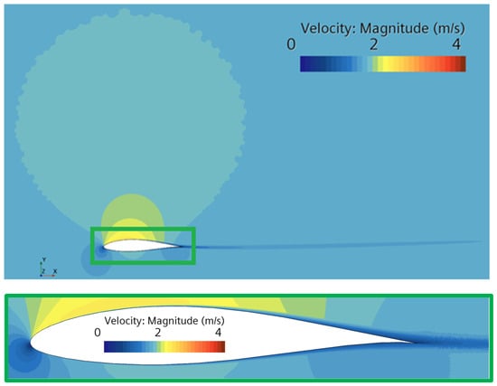
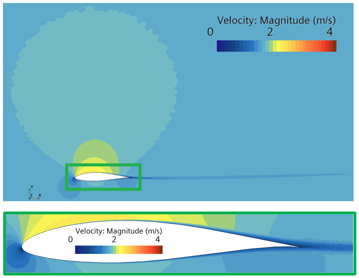
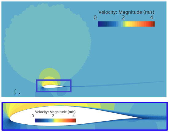
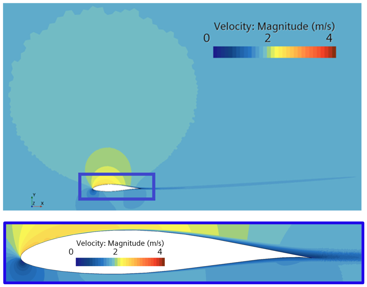
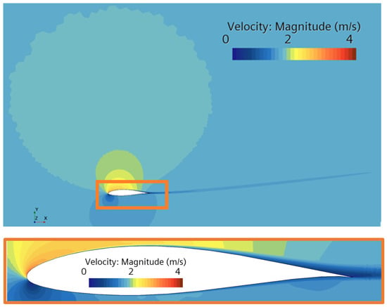
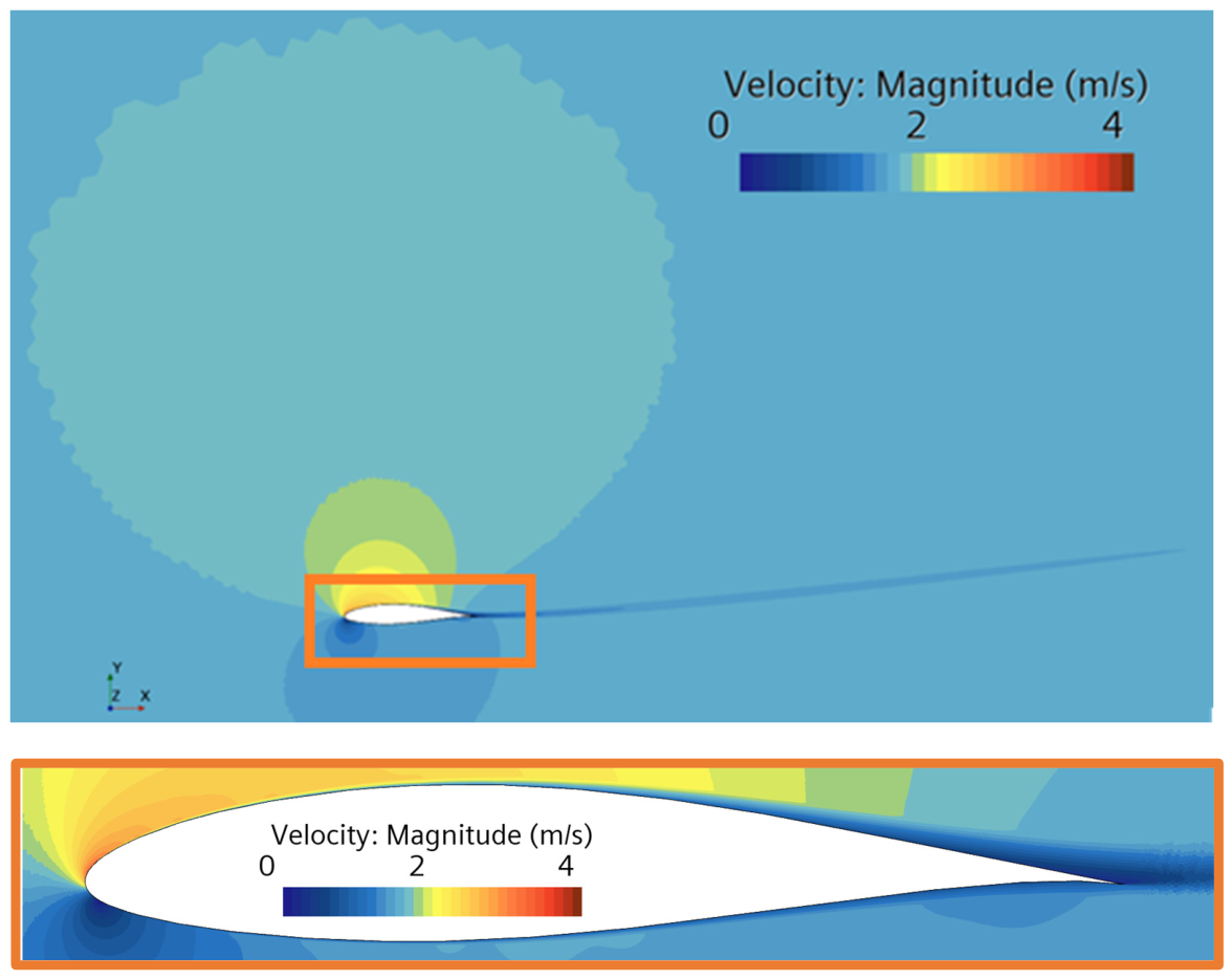
As the AOA increased, the stagnation point progressively shifted towards the lower surface, leading to increasing asymmetry in both the pressure and velocity fields. At AOA = 5°, the boundary layer on the suction side began to thicken, and mild separation was observed near the trailing edge. For AOA = 7.5° and above, substantial boundary-layer growth and wake broadening developed on the upper surface, indicating incipient or fully developed flow separation. Figure 7, Figure 8, Figure 9 and Figure 10 illustrate the velocity magnitude contours for AOAs of 2.5°, 5°, 7.5°, and 10°, respectively. This transition in flow regime plays a critical role in modifying particle trajectories and, consequently, in redistributing erosion over the hydrofoil surface.
Figure 7.
Flow velocity magnitude contour at AOA = 2.5°.
Figure 8.
Flow velocity magnitude contour at AOA = 5°.
Figure 9.
Flow velocity magnitude contour at AOA = 7.5°.
Figure 10.
Flow velocity magnitude contour at AOA = 10°.
Across all simulated cases, the near-wall flow was fully resolved through local mesh refinement, achieving y+ < 1 over the majority of the hydrofoil surface, as demonstrated in Figure 5. This level of resolution is essential for accurately capturing near-wall velocity gradients and local impact angles, both of which directly influence erosion predictions.
These hydrodynamic characteristics form the foundation for understanding particle transport mechanisms in sediment-laden flow. The manner in which particles are deflected, decelerated, or directed towards specific regions of the hydrofoil surface is governed primarily by these flow features. The resulting particle behaviour and erosion response are examined in the following sections.
3.2. Erosion Patterns and Particle–Surface Interaction Dynamics
The prediction of erosion severity across the hydrofoil surface was based on Lagrangian particle tracking coupled with the calibrated Oka erosion model. This section integrates particle residence time and computed ERs to identify the physical mechanisms governing the spatial distribution of surface degradation under varying AOAs.
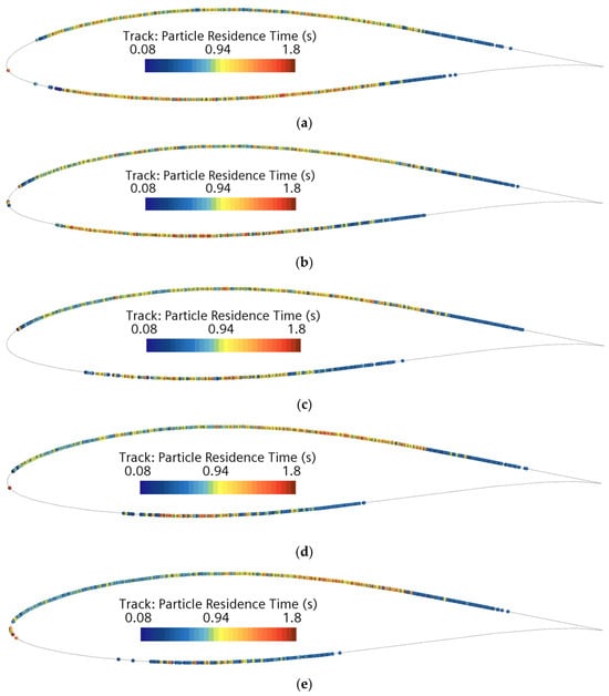
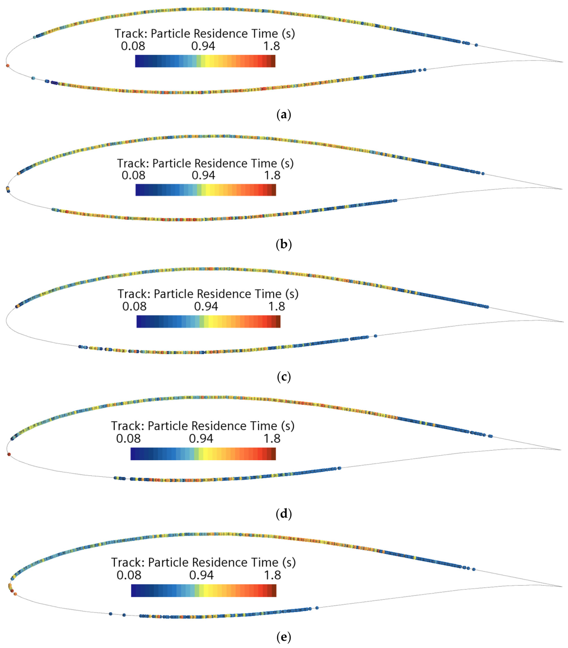
Figure 11 presents particle residence time maps for AOAs of 0°, 2.5°, 5°, 7.5°, and 10°. These visualisations indicate where particles remained near the hydrofoil surface after injection. At AOA = 0°, particle residence times are symmetrically distributed, with slightly longer residence times observed along the lower surface, while the upper surface exhibits a broader interaction region near the leading edge. As the AOA increases, a consistent trend emerges in which the interacting region on the lower face progressively diminishes. In contrast, the upper surface exhibits a larger and more persistent interaction zone across all AOAs.
Figure 11.
Particle residence time maps at AOA = (a) 0°, (b) 2.5°, (c) 5°, (d) 7.5°, and (e) 10°, showing the spatial distribution of near-wall particle interaction.
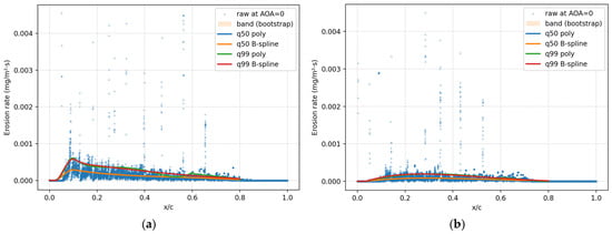
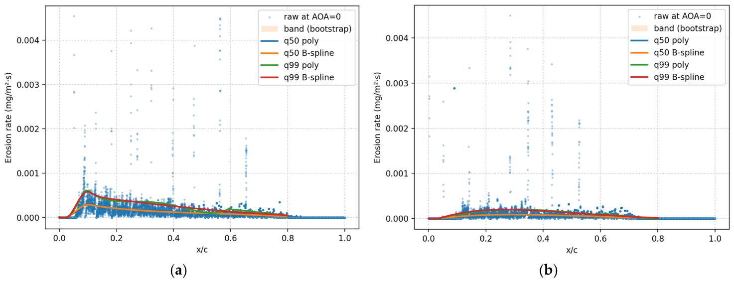
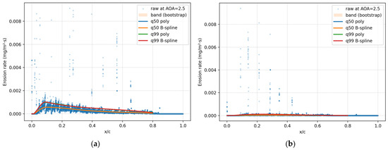
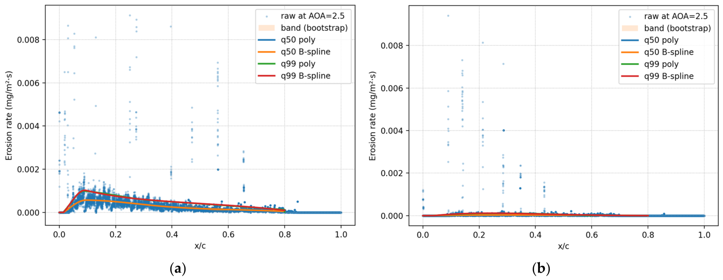
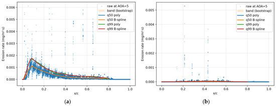
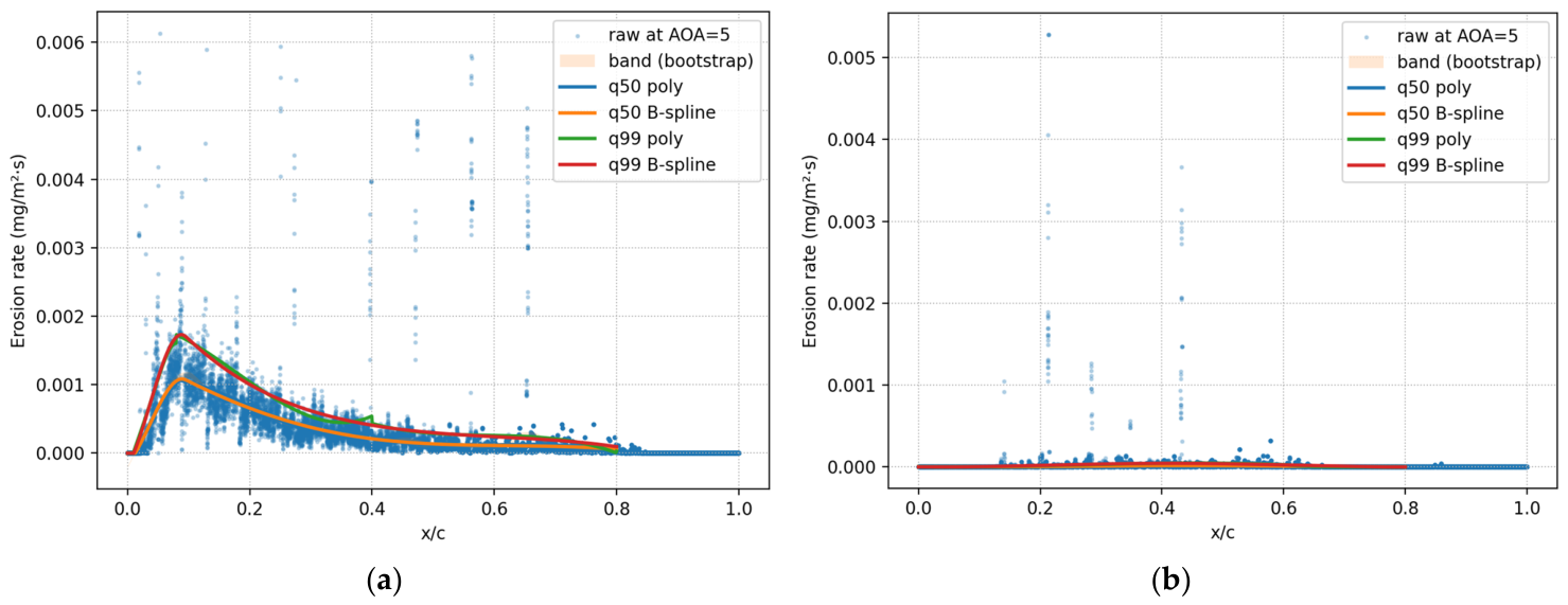
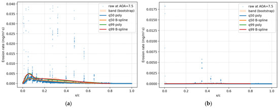
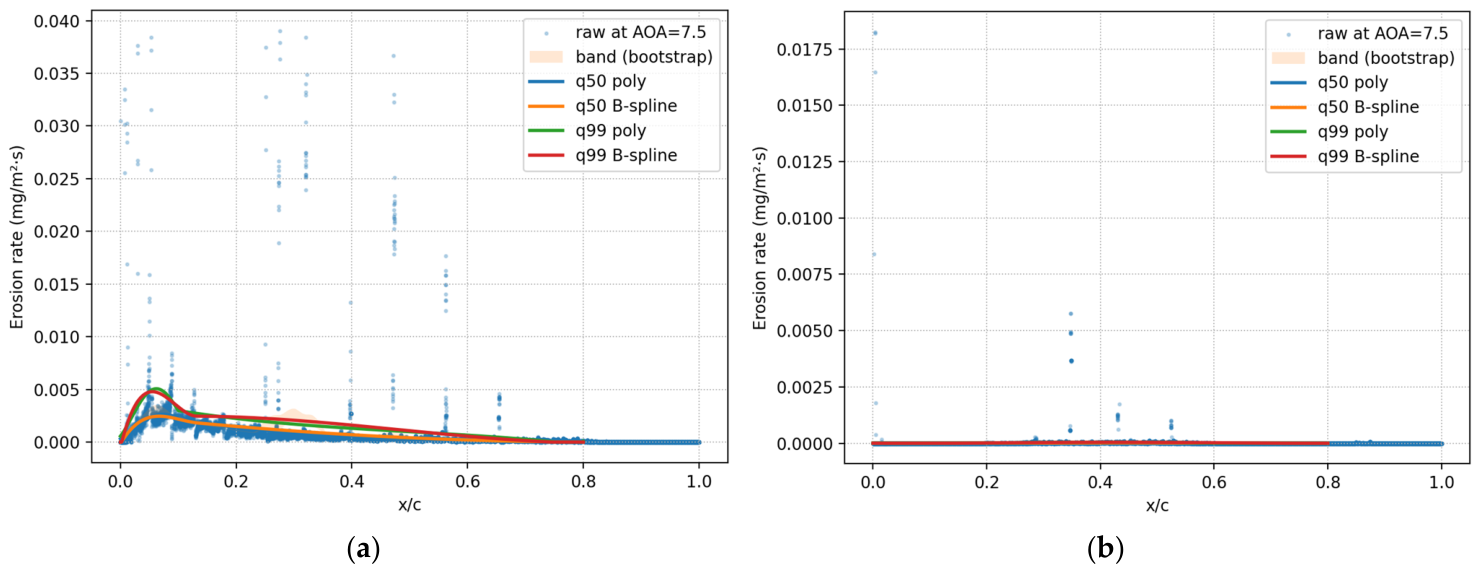
The chordwise erosion distributions shown in Figure 12, Figure 13, Figure 14, Figure 15 and Figure 16 reveal several consistent and physically meaningful trends across all investigated AOAs. Particular attention is drawn to the leading-edge region, where erosion behaviour is strongly localised and highly sensitive to flow redirection and particle impact dynamics.
Figure 12.
Erosion rate distribution at AOA = 0 on the (a) hydrofoil upper face and (b) hydrofoil lower face.
Figure 13.
Erosion rate distribution at AOA = 2.5° on the (a) hydrofoil upper face and (b) hydrofoil lower face.
Figure 14.
Erosion rate distribution at AOA = 5° on the (a) hydrofoil upper face and (b) hydrofoil lower face.
Figure 15.
Erosion rate distribution at AOA = 7.5° on the (a) hydrofoil upper face and (b) hydrofoil lower face.
Figure 16.
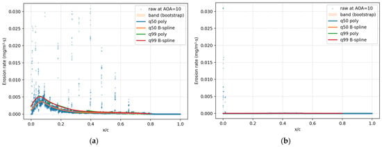
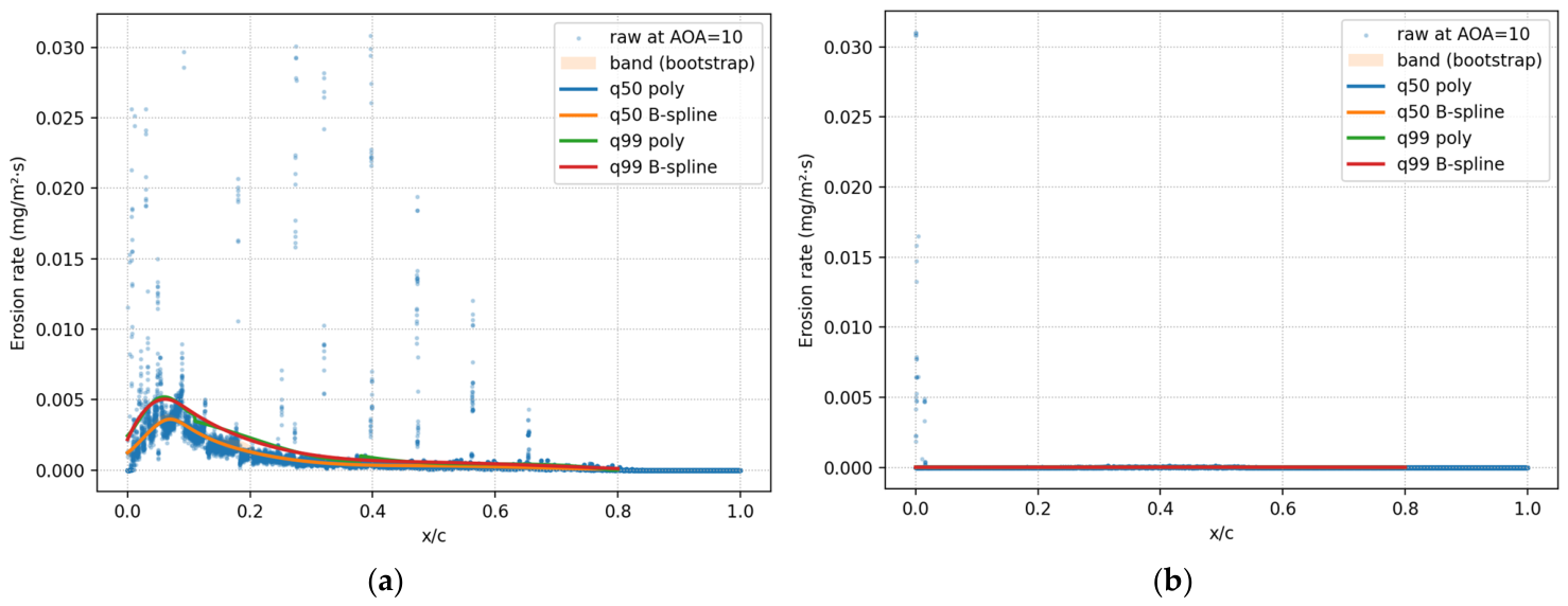
Erosion rate distribution at AOA = 10° on the (a) hydrofoil upper face and (b) hydrofoil lower face.
Across all AOAs, including the zero-angle case, the raw erosion data exhibit a distinct near-zero erosion zone extending from the stagnation point to approximately ≈ 0.04–0.06 on both upper and lower faces. This feature is consistently reproduced in all simulations and is not an artefact of data filtering or curve fitting. Instead, it reflects the physics of particle–surface interaction near the stagnation region, where particle impact velocities approach zero, and trajectories are redirected tangentially by the decelerating flow. Although particles may reside in this region, their normal impact energy is insufficient to cause measurable material removal, a behaviour previously observed and experimentally validated for FR4 glass–fibre composites under slurry-erosion conditions. Controlled 90° slurry-jet tests on FR4 produced a characteristic W-shaped erosion response [51]. Erosion was minimal or near zero at the stagnation centre and greatest immediately adjacent to it, where particles acquired greater tangential momentum and effective impact energy. This experimentally observed morphology is consistent with the near-zero erosion zone followed by a sharp rise in erosion observed in the present chordwise distributions.
Immediately downstream of this zero-erosion zone, ERs increase sharply, reaching a local maximum typically within the first 10–20% of chord length. This region corresponds to flow acceleration around the leading edge, where particles experience increasing impact velocities and more erosive impact angles. For non-zero AOAs, this peak becomes more pronounced on the upper face due to asymmetric flow acceleration and stagnation point migration. The lower face, by contrast, exhibits substantially weaker erosion levels and a more spatially confined interaction region as AOA increases.
The scatter observed in the raw erosion data reflects the inherently stochastic nature of Lagrangian particle tracking, particularly under turbulent dispersion. Isolated high-magnitude erosion points appear intermittently across the chord but do not represent systematic erosion behaviour. The q99 curves provide a stable and reproducible upper-envelope representation of erosion intensity that is robust to this stochastic scatter. They retain the near-zero erosion zone at the leading edge, reproduce the sharp rise to peak erosion, and decay smoothly along the chord. The quantile-based fitting methodology is detailed in Section 3.3.2.
Polynomial fits provide a compact representation of erosion trends but tend to exhibit local oscillations and sensitivity to segmentation choices near steep gradients. The B-spline representation, particularly for the q99 quantile, provides a smoother, more physically consistent functional form, ensuring continuity of slope and avoiding spurious extrema. For this reason, although both polynomial and B-spline fits are presented for comparison, the q99 B-spline is adopted as the final functional representative of erosion distribution for subsequent analysis and cross-AOA comparison.
Overall, these results demonstrate that erosion severity is primarily governed by local impact energy rather than by residence time alone. The persistence of a zero-erosion zone near the stagnation point, followed by a sharply localised erosion peak, is a robust and repeatable feature of sediment-induced erosion on FR4 hydrofoils. These observations form the basis for the functional erosion distributions developed in the following section, where q99 B-spline representations are used to standardise a conservative description of erosion behaviour across all AOAs.
Mechanistic Interpretation of Erosion Distribution
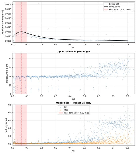
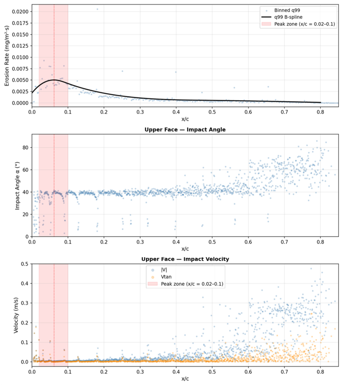
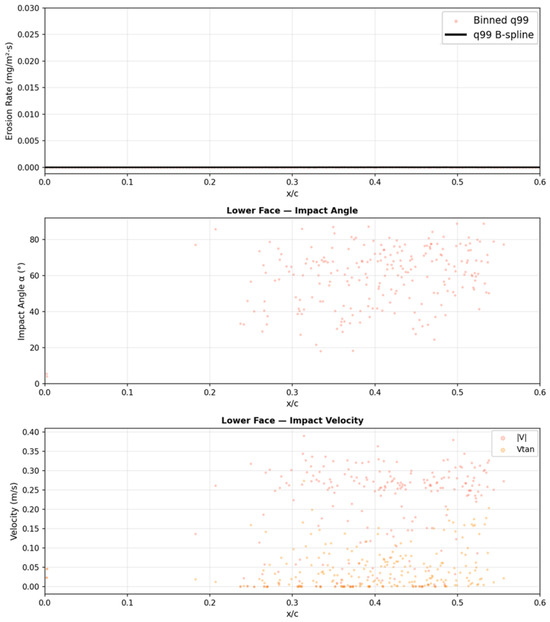
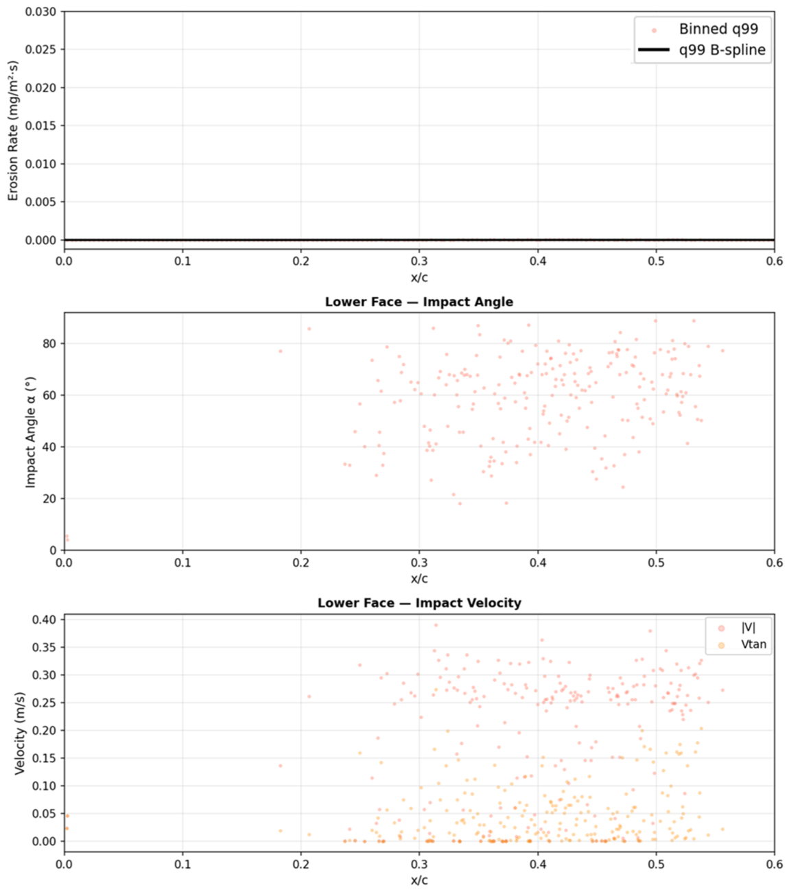
To provide mechanistic insight into the observed erosion distributions, Lagrangian particle-tracking data were extracted from the converged AOA = 10° simulation. The primary analysis concerns the chordwise erosion distributions predicted using the calibrated Oka model. The particle-tracking results are therefore presented only as supplementary mechanistic evidence from a single Lagrangian iteration of the converged solution. A statistically richer characterisation would require accumulation across multiple iterations, where increasing particle counts would yield clearer correlations between local impact conditions and erosion rates. Nevertheless, the dataset of 1176 upper-face and 229 lower-face impact records provides sufficient resolution to explain the three key features of the AOA = 10° erosion distribution, as illustrated in Figure 17 and Figure 18.
Figure 17.
Particle impact angle, velocity, and erosion rate distributions on the upper face at AOA = 10° (single Lagrangian iteration; converged).
Figure 18.
Particle impact angle, velocity, and erosion rate distributions on the lower face at AOA = 10° (single Lagrangian iteration; converged).
The lower face receives approximately five times fewer particle impacts per iteration than the upper face, as the pressure-side flow at AOA = 10° deflects the majority of incoming particles towards the suction side. Particles reaching the lower face have moderate impact angles and low velocities, so their contribution to erosion is negligible. Accordingly, the lower-face q99 B-spline peak is approximately 400 times smaller than the upper-face peak. The two impact records at the extreme leading edge of the lower face correspond to the shared geometric tip of the hydrofoil and should not be interpreted as pressure-side erosion.
On the upper face, the erosion peak centred at x/c ≈ 0.061 coincides with the region where particles first contact the suction surface as they are swept around the leading edge. Particle-tracking data show that impacts in this zone occur at mean angles of approximately 25–35°, an angular range for which the FR4-calibrated Oka model exhibits strong sensitivity, as reported in [51]. Combined with sufficient particle impact velocity in this region, this produces the highest erosion rates observed across the chord.
Beyond x/c ≈ 0.10, impact angles increase progressively as particles follow the increasingly tangential suction-side flow, reaching mean values of approximately 38–50° in the mid-chord and aft regions. Particle velocity increases in the aft region, but the nearly linear velocity exponent of the Oka model (k2 ≈ 1.008) cannot offset the reduction in angular sensitivity. The erosion rate, therefore, falls to near zero by x/c ≈ 0.40 and remains negligible farther downstream. This confirms that, for a FR4 composite under tidal sediment-laden flows, the chordwise distribution of erosion on a hydrofoil surface is primarily governed by variations in particle impact angle rather than impact velocity alone.
3.3. Functional Representation of Erosion Distribution
To express the spatial erosion trends identified in Section 3.2 in a reproducible and transferable form, the chordwise erosion distributions were represented using B-spline functions. This approach provides a compact analytical description of erosion severity while preserving the localised nature of leading-edge damage observed in the numerical results. Spline-based functional representations are widely adopted due to their compactness, local support, and numerical stability in representing spatially varying surface fields [59,60].
3.3.1. General B-Spline Formulation for Erosion Mapping
A B-spline curve of degree p is defined as a linear combination of basis functions and control coefficients [61], expressed as
where denotes the ER as a function of the normalised chordwise coordinate, x/c, n is the number of basis functions, and p is the spline degree. The basis functions are defined over a non-decreasing knot vector , which controls the curve’s locality and smoothness.
B-splines are particularly suited to erosion mapping for three reasons. First, their local support allows sharp gradients near the leading edge to be captured without inducing oscillations elsewhere along the chord. Second, continuity can be controlled explicitly through the spline degree, ensuring physically smooth erosion profiles. Third, the functional form is stable under noisy input data, which is essential when fitting ERs derived from stochastic Lagrangian particle tracking.
In the present study, cubic B-splines (p = 3) were used for all cases. Knot placement was selected to increase resolution in the leading-edge region, where erosion gradients are strongest, while maintaining smoother variation toward the mid- and trailing-edge regions. Separate B-spline functions were constructed for the upper and lower faces of the hydrofoil at each AOA.
3.3.2. Quantile-Based Fitting Strategy
The raw erosion data extracted from the CFD simulations exhibit substantial scatter due to turbulent dispersion, parcel statistics, and localised high-energy impacts. To isolate physically meaningful trends, quantile-based fitting was employed prior to spline construction.
Two quantiles were considered. The median response (q50) was used to represent the typical erosion behaviour and served primarily as a diagnostic reference. The upper-envelope response was extracted using a high-quantile formulation and treated as q99 throughout this study.
The q99 B-spline curves are therefore adopted as the final functional representation of erosion distribution. This choice provides a consistent and conservative description of erosion severity across all angles of attack, suitable for comparative analysis and subsequent model coupling.
To quantify the fidelity of the q99 B-spline representation, error metrics were computed for all investigated AOAs and both hydrofoil faces. Before fitting, values above the global 98.5th–98.7th percentile were removed as extreme outliers. Within each chordwise bin, points more than 2.5 standard deviations from the bin mean were also rejected. The 99th percentile of the remaining data within each chordwise bin was computed and subsequently smoothed using a LOWESS filter to produce a physically consistent fitting target. The coefficient of determination (R2), root mean square error (RMSE), and mean absolute error (MAE) computed between the B-spline fits and the LOWESS-smoothed q99 target are summarised in Table 3.
Table 3.
Fitting accuracy of the q99 cubic B-spline erosion distributions on the upper and lower faces of the NACA 63-415 hydrofoil across all investigated AOAs.
The upper face B-spline fits achieve R2 values between 0.742 and 0.948, confirming good to excellent fidelity across all AOAs. The lower-face metrics are more variable at non-zero angles of attack because the erosion rates are extremely low. Even where R2 is low, RMSE values of 10−6 to 10−5 mg/m2·s show that the absolute fitting errors are physically negligible.
3.3.3. Case-Specific Erosion Distribution Equations
Using the general formulation described above, erosion distribution functions were constructed separately for the upper and lower faces at each AOA investigated. For a given face and AOA, the ER can be written as
where
- is the erosion rate distribution;
- x/c is the normalised chordwise coordinate;
- are the cubic (p = 3) B-spline basis functions defined over the non-decreasing knot vector ;
- are the fitted coefficients obtained directly from the fitted B-spline model;
- n + 1 is the number of coefficients (and basis functions), determined by the knot vector length and degree: n = m − p − 1, (equivalently, n + 1 = m − p because p = 3);
- m + 1 is the number of knots.
The spline is evaluated only over its support . Outside this interval, erosion is taken as zero. Non-negativity is enforced by .
The complete set of q99 B-spline coefficients for all AOAs and for both hydrofoil faces is provided in Table 4 and Table 5.
Table 4.
Erosion Distribution Equations on the upper face of NACA 63-415 at Re = 1.6 × 10⁶ and sand size of 125 µm.
Table 5.
Erosion Distribution Equations on the lower face of NACA 63-415 at Re = 1.6 × 10⁶ and sand size of 125 µm.
These equations constitute a compact analytical representation of the erosion distributions observed in the CFD simulations.
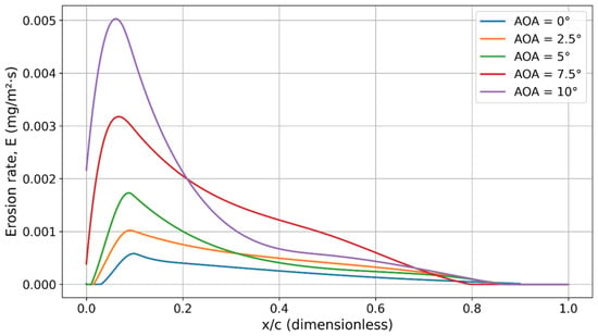
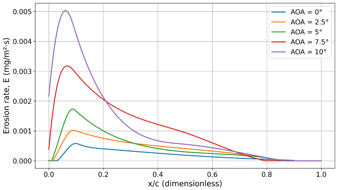
For visual comparison, the corresponding B-spline erosion curves are plotted together for each face. Figure 19 presents the q99 erosion distributions for the upper face across all AOAs, while Figure 20 shows the equivalent distributions for the lower face. These plots illustrate both the systematic increase in erosion severity with AOA and the persistent localisation of peak erosion within the leading-edge region.
Figure 19.
Erosion rate (q99 B-Spline) vs. normalised chordwise length on the hydrofoil upper face at AOA = 0~10°.
Figure 20.
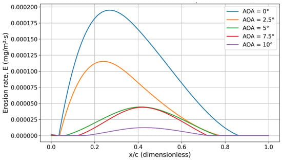
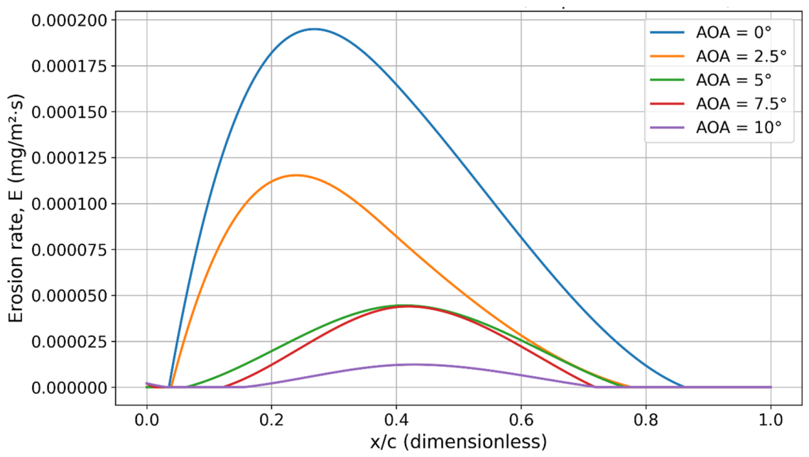
Erosion rate distributions vs. normalised chordwise length on the hydrofoil lower face at AOA = 0~10°.
4. Conclusions
This study developed a physically grounded methodology to characterise and predict leading-edge erosion on a tidal turbine hydrofoil operating under sediment-laden flow conditions. A calibrated Oka erosion model, previously validated for FR4 composite materials using standard slurry-erosion experiments, was integrated into a two-dimensional CFD framework. The hydrodynamic model was validated against experimental data for the NACA 63-415 profile reported by Bak et al., demonstrating strong agreement in lift-to-drag ratio across the investigated range of AOAs.
Erosion predictions were spatially resolved along both the upper and lower faces of the hydrofoil using Lagrangian particle tracking, enabling a detailed, surface-specific assessment of erosion behaviour. The results revealed distinct erosion characteristics depending on the AOA and surface exposure. At all AOAs, a near-zero erosion zone occurred at the stagnation region, followed by a sharply localised peak on the upper surface near the leading edge. With increasing AOA, the erosion extent increased and the peak shifted closer to the leading edge. Particle residence time maps and erosion distributions highlighted the strong influence of inflow direction, particle trajectories, and local surface orientation on erosion severity.
To quantify these trends, chordwise ER distributions were fit with polynomials and B-splines at the 99th percentile and median erosion levels. These functional representations provided a robust basis for comparative analysis across AOAs.
Overall, the methodology presented offers a scalable and transferable framework for erosion mapping in marine components; in this research, the NACA 63-415 blade section was considered. It supports the interpretation of detailed CFD erosion outputs and provides a foundation for linking erosion processes to surface degradation. The presented erosion distribution coefficients apply only to the Reynolds number, particle size and material system examined here. They should therefore be treated as outputs for the stated baseline condition rather than as universal design constants. The flow velocity of 1.6 m/s corresponds to the lower bound of the typical tidal stream velocity range of 1 to 3 m/s, providing an experimentally validated and physically grounded baseline for framework development. The calibrated Oka model supports velocity scaling through its velocity exponent k2, allowing erosion rates to be estimated at other flow velocities within the operational range without repeating the full CFD campaign. Particle-size scaling through the exponent k3 = 2.8 is reliable within and near the calibration range of 100–150 µm; additional experimental calibration data should support extrapolation to substantially different size fractions. In a design context, the chordwise erosion distribution identifies the blade surface regions most vulnerable to erosion, informing the placement of protective coatings and structural reinforcements. In a maintenance planning context, the framework supports the estimation of cumulative erosion severity under site-specific sediment and velocity conditions, enabling evidence-based scheduling of inspection and recoating intervals.
The two-dimensional framework is most applicable at mid-span locations under attached-flow conditions. Near the tip and root, and at AOAs approaching stall, three-dimensional effects, including radial-flow acceleration, hub interference, and spanwise separation, may alter local particle trajectories and erosion patterns. Future work will therefore extend the approach to three-dimensional blade geometries. A future parametric study will quantify how particle size affects impact energy, erosion severity and spatial distribution along the hydrofoil. It can build on existing FR4 erosion data for smaller sand fractions from earlier work by the research group.
Author Contributions
Conceptualisation, P.H. and S.L.; methodology, P.H. and S.L.; software, P.H.; validation, P.H. and S.L.; formal analysis, P.H.; investigation, P.H. and S.L.; resources, S.L.; data curation, P.H.; writing—original draft preparation, P.H.; writing—review and editing, S.L.; visualisation, P.H.; supervision, S.L.; funding acquisition, S.L.; All authors have read and agreed to the published version of the manuscript.
Funding
This research received no external funding.
Data Availability Statement
Data will be available upon request.
Conflicts of Interest
The authors declare no conflicts of interest.
References
- Qian, P.; Feng, B.; Liu, H.; Tian, X.; Si, Y.; Zhang, D. Review on configuration and control methods of tidal current turbines. Renew. Sustain. Energy Rev. 2019, 108, 125–139. [Google Scholar] [CrossRef] [Scilit]
- Sangiuliano, S.J. Turning of the tides: Assessing the international implementation of tidal current turbines. Renew. Sustain. Energy Rev. 2017, 80, 971–989. [Google Scholar] [CrossRef] [Scilit]
- Hassan, Q.; Viktor, P.; Al-Musawi, T.J.; Ali, B.M.; Algburi, S.; Alzoubi, H.M.; Al-Jiboory, A.K.; Sameen, A.Z.; Salman, H.M.; Jaszczur, M. The renewable energy role in the global energy Transformations. Renew. Energy Focus 2024, 48, 100545. [Google Scholar] [CrossRef] [Scilit]
- Nan, J.; Zhi, C.; Meng, J.; Miao, M.; Yu, L. Seawater aging effect on fiber-reinforced polymer composites: Mechanical properties, aging mechanism, and life prediction. Text. Res. J. 2023, 93, 3393–3413. [Google Scholar] [CrossRef] [Scilit]
- Prashar, G.; Vasudev, H.; Thakur, L. Performance of different coating materials against slurry erosion failure in hydrodynamic turbines: A review. Eng. Fail. Anal. 2020, 115, 104622. [Google Scholar] [CrossRef] [Scilit]
- Sun, J.; Ge, X.; Zhou, Y.; Liu, D.; Liu, J.; Li, G.; Zheng, Y. Research on synergistic erosion by cavitation and sediment: A review. Ultrason. Sonochemistry 2023, 95, 106399. [Google Scholar] [CrossRef] [Scilit]
- Groucott, S.; Pugh, K.; Zekos, I.; Stack, M.M. A study of raindrop impacts on a wind turbine material: Velocity and impact angle effects on erosion maps at various exposure times. Lubricants 2021, 9, 60. [Google Scholar] [CrossRef] [Scilit]
- Hassan, E.; Zekos, I.; Jannson, P.; Pecor, T.; Floreani, C.; Robert, C.; Ó Brádaigh, C.M.; Stack, M.M. Erosion mapping of through-thickness toughened powder epoxy gradient glass-fiber-reinforced polymer (GFRP) plates for tidal turbine blades. Lubricants 2021, 9, 22. [Google Scholar] [CrossRef] [Scilit]
- Draycott, S.; Sellar, B.; Davey, T.; Noble, D.R.; Venugopal, V.; Ingram, D.M. Capture and simulation of the ocean environment for offshore renewable energy. Renew. Sustain. Energy Rev. 2019, 104, 15–29. [Google Scholar] [CrossRef] [Scilit]
- Clark, C.E.; DuPont, B. Reliability-based design optimisation in offshore renewable energy systems. Renew. Sustain. Energy Rev. 2018, 97, 390–400. [Google Scholar] [CrossRef] [Scilit]
- Neill, S.P. Fundamentals of Ocean Renewable Energy: Generating Electricity from the Sea; Academic Press: Cambridge, MA, USA, 2018. [Google Scholar]
- Izadi Gonabadi, H. Performance of Low Cost Composites for Tidal Turbine Applications. Ph.D. Thesis, Newcastle University, Newcastle upon Tyne, UK, 2019. [Google Scholar]
- Zhou, Z.; Benbouzid, M.; Charpentier, J.-F.; Scuiller, F.; Tang, T. Developments in large marine current turbine technologies—A review. Renew. Sustain. Energy Rev. 2017, 71, 852–858. [Google Scholar] [CrossRef] [Scilit]
- Neill, S.P.; Haas, K.A.; Thiébot, J.; Yang, Z. A review of tidal energy—Resource, feedbacks, and environmental interactions. J. Renew. Sustain. Energy 2021, 13, 062702. [Google Scholar] [CrossRef] [Scilit]
- Finkl, C.W.; Charlier, R. Electrical power generation from ocean currents in the Straits of Florida: Some environmental considerations. Renew. Sustain. Energy Rev. 2009, 13, 2597–2604. [Google Scholar] [CrossRef] [Scilit]
- Khan, M.J.; Bhuyan, G.; Iqbal, M.T.; Quaicoe, J.E. Hydrokinetic energy conversion systems and assessment of horizontal and vertical axis turbines for river and tidal applications: A technology status review. Appl. Energy 2009, 86, 1823–1835. [Google Scholar] [CrossRef] [Scilit]
- Zilic de Arcos, F. Hydrodynamics of Highly-Loaded Axial Flow Tidal Rotors. Ph.D. Thesis, University of Oxford, Oxford, UK, 2021. [Google Scholar]
- Jing, F.-M.; Ma, W.-J.; Zhang, L.; Wang, S.-Q.; Wang, X.-H. Experimental study of hydrodynamic performance of full-scale horizontal axis tidal current turbine. J. Hydrodyn. Ser. B 2017, 29, 109–117. [Google Scholar] [CrossRef] [Scilit]
- Capone, A.; DiFelice, F.; Salvatore, F.; Maddukkari, H.; Kaufmann, N.; Starzmann, R. Impact of cavitation and inflow perturbation on the performance of a horizontal-axis tidal turbine. J. Ocean Eng. Mar. Energy 2023, 9, 731–743. [Google Scholar] [CrossRef] [Scilit]
- Bahaj, A.S.; Molland, A.F.; Chaplin, J.R.; Batten, W.M.J. Power and thrust measurements of marine current turbines under various hydrodynamic flow conditions in a cavitation tunnel and a towing tank. Renew. Energy 2007, 32, 407–426. [Google Scholar] [CrossRef] [Scilit]
- Parsi, M.; Al-Sarkhi, A.; Kara, M.; Sharma, P.; McLaury, B.S.; Shirazi, S.A. A new dimensionless number for solid particle erosion in natural gas elbows. Wear 2017, 390–391, 80–83. [Google Scholar] [CrossRef] [Scilit]
- Adedeji, O.E.; Yu, W.; Sanders, R.S. Analysis of local wear variables for high-precision erosion modelling in complex geometries. Wear 2019, 426–427, 562–569. [Google Scholar] [CrossRef] [Scilit]
- Messa, G.V.; Malavasi, S. A CFD-based method for slurry erosion prediction. Wear 2018, 398–399, 127–145. [Google Scholar] [CrossRef] [Scilit]
- Wan, X.; Dong, M.; Xu, M.; Fan, C.; Mou, J.; Han, S. Numerical Prediction of Solid Particle Erosion in Jet Pumps Based on a Calibrated Model. Energies 2024, 17, 5720. [Google Scholar] [CrossRef] [Scilit]
- Sezen, S. Marine Propeller Hydrodynamic and Hydroacoustic Performance with Roughness Effects. Ph.D. Thesis, University of Strathclyde, Glasgow, UK, 2022. [Google Scholar] [CrossRef]
- Gao, Y.; Liu, H.; Lin, Y.; Gu, Y.; Wang, S. Numerical investigation of the erosion behavior in blades of tidal current turbine. J. Renew. Sustain. Energy 2022, 14, 044502. [Google Scholar] [CrossRef] [Scilit]
- Wang, Y.; Wang, L.; Duan, C.; Zheng, J.; Liu, Z.; Ma, G. CFD simulation on wind turbine blades with leading edge erosion. J. Theor. Appl. Mech. 2021, 59, 579–593. [Google Scholar] [CrossRef] [Scilit] [PubMed]
- El-Maaty, A.A.; Abdallah, H.; Kotb, M.; Ben-Mansour, R.; Alatawi, E. Numerical investigation of sand erosion rate in a horizontal axis wind turbine. Heliyon 2024, 10, e27676. [Google Scholar] [CrossRef] [Scilit] [PubMed]
- Vimalakanthan, K.; van der Mijle Meijer, H.; Bakhmet, I.; Schepers, G. Computational fluid dynamics (CFD) modeling of actual eroded wind turbine blades. Wind Energy Sci. 2023, 8, 41–69. [Google Scholar] [CrossRef] [Scilit]
- Tempelis, A.; Mishnaevsky, L., Jr. Surface roughness evolution of wind turbine blade subject to rain erosion. Mater. Des. 2023, 231, 112011. [Google Scholar] [CrossRef] [Scilit]
- Carraro, M.; De Vanna, F.; Zweiri, F.; Benini, E.; Heidari, A.; Hadavinia, H. CFD modeling of wind turbine blades with eroded leading edge. Fluids 2022, 7, 302. [Google Scholar] [CrossRef] [Scilit]
- Wu, R.-j.; Chen, J.-j.; Liu, W.-b.; Chen, Y.; Xia, J. Influence of erosion damage on the spatiotemporal deterioration of marine RC structures. Eng. Fail. Anal. 2024, 165, 108747. [Google Scholar] [CrossRef] [Scilit]
- Wan, D.; Chen, S.; Li, D.; Zhen, Q.; Zhang, B. Sand-Laden Wind Erosion Pair Experimental Analysis of Aerodynamic Performance of the Wind Turbine Blades. Energies 2024, 17, 2279. [Google Scholar] [CrossRef] [Scilit]
- Wood, R.J.K.; Bahaj, A.S.; Turnock, S.R.; Wang, L.; Evans, M. Tribological design constraints of marine renewable energy systems. Proc. R. Soc. A 2010, 368, 4807–4827. [Google Scholar] [CrossRef] [Scilit] [PubMed]
- Song, S.; Demirel, Y.K.; Atlar, M.; Shi, W. Prediction of the fouling penalty on the tidal turbine performance and development of its mitigation measures. Appl. Energy 2020, 276, 115498. [Google Scholar] [CrossRef] [Scilit]
- Habibi, P.; Abad, F.; Dai, S.; Mehmanparast, A.; Lotfian, S. Failure analysis of tidal turbine blades: Understanding erosion mechanisms and their impact on structural integrity. Eng. Fail. Anal. 2025, 182, 110045. [Google Scholar] [CrossRef] [Scilit]
- Sareen, A.; Sapre, C.A.; Selig, M.S. Effects of leading edge erosion on wind turbine blade performance. Wind Energy 2014, 17, 1531–1542. [Google Scholar]
- Kelly, J.; Vogel, C.; Willden, R. Impact and mitigation of blade surface roughness effects on wind turbine performance. Wind Energy 2022, 25, 660–677. [Google Scholar] [CrossRef] [Scilit]
- Gnanavelu, A.; Kapur, N.; Neville, A.; Flores, J.; Ghorbani, N. A numerical investigation of a geometry independent integrated method to predict erosion rates in slurry erosion. Wear 2011, 271, 712–719. [Google Scholar] [CrossRef] [Scilit]
- Karimi, S.; Shirazi, S.A.; McLaury, B.S. Predicting fine particle erosion utilising computational fluid dynamics. Wear 2017, 376–377, 1130–1137. [Google Scholar] [CrossRef] [Scilit]
- Pryor, S.C.; Coburn, J.J.; Barthelmie, R.J. Spatiotemporal Variability in Wind Turbine Blade Leading Edge Erosion. Energies 2025, 18, 425. [Google Scholar] [CrossRef] [Scilit]
- Wang, H.; Chen, B. Investigation of the Computational Framework of Leading-Edge Erosion for Wind Turbine Blades. Energies 2025, 18, 2146. [Google Scholar] [CrossRef] [Scilit]
- Habibi, P.; Algaddaime, T.F.; Abad, F.; Stack, M.M.; Mehmanparast, A.; Brennan, F.; Lotfian, S. Structural integrity evolution of composite tidal turbine materials: Correlating surface roughness with progressive erosive damage. Theor. Appl. Fract. Mech. 2025, 139, 105076. [Google Scholar] [CrossRef] [Scilit]
- Menter, F.R. Two-equation eddy-viscosity turbulence models for engineering applications. AIAA J. 1994, 32, 1598–1605. [Google Scholar] [CrossRef] [Scilit]
- Schiller, V.L. Uber die grundlegenden Berechnungen bei der Schwerkraftaufbereitung. Z. Ver. Dtsch. Ingenieure 1933, 77, 318–321. [Google Scholar]
- Siemens Digital Industries Software. Simcenter STAR-CCM+ User Guide; Siemens Digital Industries Software: Plano, TX, USA, 2025. [Google Scholar]
- Oka, Y.I.; Okamura, K.; Yoshida, T. Practical estimation of erosion damage caused by solid particle impact: Part 1: Effects of impact parameters on a predictive equation. Wear 2005, 259, 95–101. [Google Scholar] [CrossRef] [Scilit]
- Oka, Y.; Yoshida, T. Practical estimation of erosion damage caused by solid particle impact: Part 2: Mechanical properties of materials directly associated with erosion damage. Wear 2005, 259, 102–109. [Google Scholar] [CrossRef] [Scilit]
- Abbott, I.H.; Von Doenhoff, A.E. Theory of Wing Sections: Including a Summary of Airfoil Data; Courier Corporation: North Chelmsford, MA, USA, 2012. [Google Scholar]
- Bak, C.; Fuglsang, P.; Johansen, J.; Antoniou, I. Wind Tunnel Tests of the NACA 63-415 and a Modified NACA 63-415 Airfoil. 2000. Available online: https://orbit.dtu.dk/en/publications/wind-tunnel-tests-of-the-naca-63-415-and-a-modified-naca-63-415-a/ (accessed on 28 June 2026).
- Habibi, P.; Lotfian, S. Calibration and validation of slurry erosion models for glass fibre composites in marine energy systems. J. Mar. Sci. Eng. 2025, 13, 1602. [Google Scholar] [CrossRef] [Scilit]
- Mansouri, A. A Combined CFD-Experimental Method for Developing an Erosion Equation for Both Gas-Sand and Liquid-Sand Flows. Ph.D. Thesis, The University of Tulsa, Tulsa, OK, USA, 2016. [Google Scholar]
- Grant, G.; Tabakoff, W. Erosion prediction in turbomachinery resulting from environmental solid particles. J. Aircr. 1975, 12, 471–478. [Google Scholar] [CrossRef] [Scilit]
- Arabnejad, H.; Mansouri, A.; Shirazi, S.A.; McLaury, B.S. Abrasion erosion modeling in particulate flow. Wear 2017, 376–377, 1194–1199. [Google Scholar] [CrossRef] [Scilit]
- Arabnejad, H.; Mansouri, A.; Shirazi, S.A.; McLaury, B.S. Development of mechanistic erosion equation for solid particles. Wear 2015, 332–333, 1044–1050. [Google Scholar] [CrossRef] [Scilit]
- Arabnejad, H.; Mansouri, A.; Shirazi, S.; McLaury, B. Evaluation of solid particle erosion equations and models for oil and gas industry applications. In Proceedings of the SPE Annual Technical Conference and Exhibition, Houston, TX, USA, 28–30 September 2015. [Google Scholar] [CrossRef] [Scilit]
- Sawant, A. Solid Particle Erosion Modelling Using CFD Techniques. Ph.D. Thesis, University of Warwick, Coventry, UK, 2021. [Google Scholar]
- Mansouri, A.; Arabnejad, H.; Shirazi, S.A.; McLaury, B.S. A combined CFD/experimental methodology for erosion prediction. Wear 2015, 332–333, 1090–1097. [Google Scholar] [CrossRef] [Scilit]
- Wei, Z.; Wei, X. Scalable field-aligned reparameterisation for trimmed NURBS. Eng. Comput. 2025, 41, 2043–2067. [Google Scholar] [CrossRef] [Scilit]
- Amiri-Simkooei, A.; Esmaeili, F.; Lindenbergh, R. Least squares B-spline approximation with applications to geospatial point clouds. Measurement 2025, 248, 116887. [Google Scholar] [CrossRef] [Scilit]
- Piegl, L.; Tiller, W. The NURBS Book; Springer Science & Business Media: Berlin/Heidelberg, Germany, 2012. [Google Scholar]



Disclaimer/Publisher’s Note: The statements, opinions and data contained in all publications are solely those of the individual author(s) and contributor(s) and not of MDPI and/or the editor(s). MDPI and/or the editor(s) disclaim responsibility for any injury to people or property resulting from any ideas, methods, instructions or products referred to in the content. |
© 2026 by the authors. Licensee MDPI, Basel, Switzerland. This article is an open access article distributed under the terms and conditions of the Creative Commons Attribution (CC BY) license.