


Abstract
Accurate three-dimensional temperature and salinity initial fields are essential for regional short-term ocean forecasting, but subsurface constraints remain limited in the Western Indian Ocean because in situ profiles are sparse and satellite observations mainly describe the sea surface. This study evaluated a method to improve short-term forecasts by assimilating pretrained language model (PLM)-reconstructed thermohaline fields into the Finite Volume Community Ocean Model with a three-dimensional variational data assimilation scheme (FVCOM–3DVAR). The method was applied to the Western Indian Ocean, covering 15° S–10° N, 33° E–60° E. A non-assimilation control experiment (Control_run), Modular Ocean Data Assimilation System assimilation (MODAS_ass), and PLM reconstructed-field assimilation (PLM_ass) were conducted to evaluate the forecast performance with 5-day rolling forecasts. World Ocean Database (WOD) profiles were used for profile-based validation, and Copernicus Marine Environment Monitoring Service (CMEMS) gridded fields were used for spatially continuous reference evaluation in February, May, August, and November 2021. The results demonstrated that PLM_ass produced lower temperature and salinity root-mean-square errors (RMSEs) than Control_run and MODAS_ass at most depths and lead times. Relative to Control_run, PLM_ass reduced mean temperature RMSE by 28.0% at 100–200 m and mean salinity RMSE by 23.5% at 0–100 m; compared with MODAS_ass, the reductions were approximately 16.6% and 14.2%, respectively. Spatial diagnostics showed variable-, depth-, and region-dependent impacts with the most robust improvement in thermocline temperature forecasts. This study provides a feasible pathway for incorporating AI-reconstructed subsurface information into regional ocean forecasting systems under sparse observation conditions.
1. Introduction
Accurate short-term prediction of three-dimensional temperature and salinity fields is a fundamental component of regional ocean forecasting. Temperature and salinity jointly determine seawater density, vertical stratification, baroclinic pressure gradients, mixed-layer evolution, and the subsequent adjustment of upper-ocean and subsurface hydrographic structures. Errors in the initial thermohaline state can propagate during model integration and affect short-term forecasts of temperature, salinity, circulation, and sea level, particularly in regions with strong vertical gradients and active mesoscale variability [1,2,3]. Therefore, improving the initial three-dimensional thermohaline structure is essential for reducing short-term forecast errors in regional ocean prediction systems.
Operational and regional ocean forecasting systems commonly combine numerical circulation models with data assimilation to constrain the model state using available observations [3,4,5]. Global and basin-scale systems, such as HYCOM–NCODA, have demonstrated the value of multivariate ocean data assimilation for improving ocean analyses and short-term forecasts [2,6]. At the regional scale, variational data assimilation has also been implemented in several widely used ocean models. For example, ROMS has been coupled with both three-dimensional variational assimilation and mature four-dimensional variational assimilation systems for regional ocean prediction and observation impact studies [7,8]. The Navy Coastal Ocean Model has also been extended with a 4D-Var assimilation framework for coastal and regional applications [9]. In coastal hydrodynamic prediction, ADCIRC has been combined with ensemble-based assimilation methods for storm-surge and water-level forecasting, although its main application differs from the three-dimensional thermohaline initialization considered here [10]. Recent ADCIRC studies have emphasized the role of unstructured mesh design and local mesh refinement in resolving global-to-coastal storm tide dynamics [11], while high-resolution tidal simulations in narrow straits, such as La Perouse Strait, further demonstrate the importance of grid resolution and coastal geometry representation for tide-resolving models [12]. These studies indicate that the effectiveness of data-assimilative forecast systems depends not only on the dynamical core but also on observation availability, error covariance specification, and the consistency between observations and model dynamics [3,13]. Satellite sea-surface temperature and altimetry provide broad spatial constraints on the surface ocean [14,15], whereas Argo and other in situ profiles provide direct vertical constraints on subsurface stratification and thermocline structure [16,17,18]. However, when profile observations are sparse or unevenly distributed, surface observations alone are insufficient to fully constrain the three-dimensional temperature and salinity structure [3,19].
This limitation is particularly important in the Western Indian Ocean. The region is strongly affected by monsoon-driven circulation and the seasonal reversal of the Somali Current [20,21,22]. It also contains dynamically active features such as the Great Whirl, the Seychelles–Chagos Thermocline Ridge, mesoscale eddies, coastal upwelling, and water mass exchange [23,24,25,26]. These processes produce pronounced thermocline variability and spatially heterogeneous salinity structures, making short-term temperature and salinity forecasts sensitive to the initial three-dimensional thermohaline state [24,25,27]. Although satellite observations provide continuous sea-surface information, they cannot directly observe the subsurface thermohaline structure. Direct in situ profiles provide vertical temperature and salinity observations, but their sampling remains uneven in space and time, especially in dynamically active and coastal regions [16,18,28]. Consequently, conventional observation-based initialization may still be insufficient to constrain thermocline displacement and subsurface salinity variability in the Western Indian Ocean.
Reconstructed or synthetic three-dimensional thermohaline products provide a potential supplementary source of subsurface information. Traditional systems such as the Modular Ocean Data Assimilation System (MODAS) infer subsurface temperature and salinity fields from sea-surface temperature, sea-surface height anomaly, and historical thermohaline relationships [29]. Earlier observation-based approaches combined Argo and remote sensing data to estimate three-dimensional temperature fields [30], and more recent data-driven studies have shown that sea-surface information can be used to infer subsurface temperature and salinity structures [31,32,33,34]. Neural network, convolutional, and transformer-based approaches have further been applied to reconstruct subsurface temperature and salinity fields from multi-source surface observations, including remote sensing and in situ constraints [34,35,36,37,38,39,40,41]. However, reconstruction accuracy alone does not necessarily imply forecast improvement after assimilation. Once a reconstructed field is introduced into a dynamical model as pseudo-observations, its forecast impact depends on its error structure, spatial coherence, consistency with the model background, prescribed observation error covariance, and subsequent adjustment of the numerical model [3,42]. Therefore, the practical value of AI-reconstructed thermohaline fields should be evaluated not only by static reconstruction accuracy but also by their ability to reduce short-term forecast errors after assimilation.
Based on this motivation, this study evaluates the forecast impact of assimilating pretrained language model (PLM)-reconstructed three-dimensional temperature and salinity fields into the Finite Volume Community Ocean Model with three-dimensional variational data assimilation (FVCOM–3DVAR) in the Western Indian Ocean. Three comparative experiments are designed: a non-assimilation control experiment (Control_run), a MODAS thermohaline field assimilation experiment (MODAS_ass), and a PLM-reconstructed-field assimilation experiment (PLM_ass). Five-day rolling forecasts are conducted for representative seasonal months in 2021. Forecast skill is evaluated using World Ocean Database (WOD) profiles and Copernicus Marine Environment Monitoring Service (CMEMS) gridded reference fields [18,43]. The objective of this study is not to replace direct in situ observations or conventional assimilation products, but to examine whether PLM-reconstructed thermohaline fields can serve as supplementary pseudo-observational constraints for improving short-term regional temperature and salinity forecasts under sparse subsurface observations.
The remainder of this paper is organized as follows. Section 2 describes the study region, datasets, FVCOM–3DVAR configuration, assimilation experiments, and evaluation metrics. Section 3 presents the forecast error characteristics of Control_run, MODAS_ass, and PLM_ass based on WOD profile verification, lead-time–depth RMSE analysis, and spatial error diagnostics. Section 4 discusses the physical interpretation, limitations, and methodological implications of assimilating reconstructed thermohaline fields. Section 5 summarizes the main conclusions.
2. Data and Methods
2.1. Study Region and Datasets
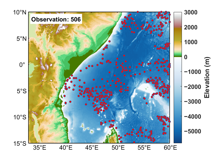
The study region is the Western Indian Ocean, covering 15° S–10° N and 33° E–60° E, including the Somali coastal area, the equatorial Western Indian Ocean, the northern Mozambique Channel, and the waters northwest of Madagascar. The spatial distribution of all available WOD profile stations within the study domain is shown in Figure 1. Under the combined influence of monsoon forcing, boundary currents, mesoscale eddies, and water mass transport, the upper-ocean and thermocline layer temperature and salinity structures in this region exhibit pronounced seasonal variability and spatial heterogeneity [20,24,25,44]. These characteristics make the region suitable for assessing the impact of thermohaline initialization on short-term three-dimensional temperature and salinity forecasts.
Figure 1.
Topography of the Western Indian Ocean and distribution of WOD profile stations.
The model forcing and boundary datasets include ETOPO1 bathymetry, GSHHG coastline data, ERA5 atmospheric forcing, TPXO tidal forcing, and Copernicus Marine Environment Monitoring Service (CMEMS) ocean initial and open-boundary fields [43,45,46,47,48]. These datasets were interpolated onto the FVCOM unstructured grid and its vertical coordinate system to construct the regional short-term forecast system.
The assimilated datasets were PLM-reconstructed three-dimensional thermohaline fields and MODAS three-dimensional thermohaline fields. Both datasets had a horizontal resolution of 1/8° and contained temperature and salinity fields at 19 standard depth levels, namely, 0, 20, 30, 50, 70, 100, 150, 200, 250, 300, 400, 500, 700, 1000, 1250, 1500, 2000, 2500, and 3000 m. The MODAS thermohaline field was used as a traditional statistical reconstruction baseline [29]. In the assimilation experiments, both products were used as daily thermohaline pseudo-observations after preprocessing.
The PLM-reconstructed thermohaline product was generated from same-day sea-surface information, including sea surface temperature, sea level anomaly, and temporal indicators, and the model mapped these surface constraints to three-dimensional temperature and salinity fields at the 19 standard depth levels listed above. In brief, the surface variables were first converted into spatial tokens through a two-dimensional convolutional embedding module and then processed by Transformer blocks initialized from a pretrained GPT-2 architecture. The original text-embedding layer, causal language modeling head, and autoregressive prediction setting were removed because the target task was oceanic field reconstruction rather than text generation. Low-rank adaptation was applied to selected attention projections, and a unified three-dimensional decoder was used to generate the temperature and salinity fields. In the present FVCOM–3DVAR experiments, the PLM product was introduced only as an external AI-reconstructed pseudo-observation source and was not retrained within the dynamical assimilation system. In the companion reconstruction study, independent profile-based evaluation showed that, compared with MODAS, the PLM product reduced thermocline layer temperature RMSE by approximately 0.08–0.24 °C over 50–200 m and near-surface salinity RMSE by approximately 0.02–0.23 psu over 0–150 m. A detailed description of the PLM architecture and training procedure is provided in the companion manuscript entitled "PLM-based Reconstruction of Temperature and Salinity in the Western Indian Ocean".
Before entering the assimilation system, the PLM and MODAS thermohaline fields were clipped to 15° S–10° N and 33° E–60° E, and missing values were removed. The regular latitude–longitude thermohaline fields were then horizontally interpolated onto FVCOM unstructured grid nodes and vertically interpolated from standard depth levels to sigma layers. This procedure produced three-dimensional thermohaline pseudo-observations consistent with the model grid and vertical coordinate.
Data preprocessing, interpolation, and statistical calculation were performed using Python 3.11.8 (Python Software Foundation, https://www.python.org/). The PLM reconstruction framework was implemented using PyTorch 2.4.0 (https://pytorch.org/). Figure plotting and visualization were performed using MATLAB R2022b (https://www.mathworks.com/products/matlab.html, accessed on 31 December 2025). The regional numerical forecast was conducted using FVCOM v5.0 (http://fvcom.smast.umassd.edu/).
The validation datasets include World Ocean Database (WOD) in situ temperature and salinity profiles and CMEMS three-dimensional thermohaline fields [18,43]. WOD profiles were used for independent station-based verification, whereas CMEMS was used for gridded error evaluation of spatially continuous fields.
2.2. FVCOM–3DVAR Forecast System
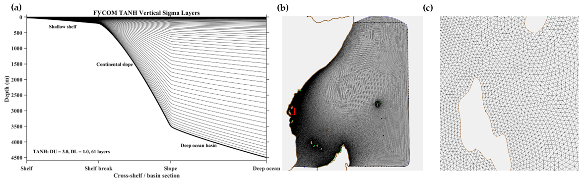
FVCOM was used to construct the regional short-term forecast system for the Western Indian Ocean. The model solves the three-dimensional free-surface primitive equations on an unstructured triangular grid, which allows it to represent the complex coastlines, islands, and open-boundary geometry of the study region [49]. The model domain covers 15° S–10° N and 33° E–60° E. The horizontal grid contains 77,228 nodes and 152,149 triangular elements, with a horizontal resolution of approximately 8–20 km. Two open boundaries were specified. Tidal forcing was prescribed at the two open boundaries using harmonic constants from the TPXO global tidal model [48]. The selected constituents included M2, S2, N2, K2, K1, O1, P1, Q1, Mm, Mf, M4, MN4, MS4, and 2N2. These harmonic constants were interpolated onto the FVCOM open-boundary nodes and used to reconstruct time-varying tidal elevations and tidal current boundary conditions. In the vertical direction, 61 terrain-following sigma layers were used, with TANH stretching parameters of DU = 3.0 and DL = 1.0 [50]. Vertical mixing was represented using the Mellor–Yamada level-2.5 turbulence closure scheme [51]. The resulting vertical sigma layer distribution, full-domain horizontal unstructured triangular mesh, and a zoomed-in view of the local triangular elements are shown in Figure 2.
Figure 2.
FVCOM vertical sigma layer structure and horizontal unstructured mesh configuration. (a) Schematic diagram of the FVCOM TANH vertical sigma layer distribution with 61 sigma layers and stretching parameters of DU = 3.0 and DL = 1.0; (b) full-domain unstructured triangular mesh of the FVCOM computational domain in the Western Indian Ocean; (c) enlarged view of the local mesh area marked by the red box in panel (b), illustrating the triangular grid elements in greater detail.
The three forecast experiments used the same model grid, bathymetry, open-boundary conditions, atmospheric forcing, tidal forcing, time step, vertical coordinate, and turbulence parameterization. Therefore, differences among the experiments mainly arose from the different assimilated data sources.
A three-dimensional variational data assimilation method was used to update the initial temperature and salinity fields of the model [7,52]. The cost function can be written as:
where denotes the analysis field obtained by minimizing the cost function, is the background field derived from the prior model state, represents the observation vector, is the observation operator used to project model variables onto the observation space, and and denote the background error and observation error covariance matrices, respectively.
During each assimilation cycle, the FVCOM temperature and salinity forecasts before assimilation were used as the background fields. The PLM and MODAS three-dimensional thermohaline fields were introduced into the 3DVAR system as gridded pseudo-observations. The system calculated temperature or salinity analysis increments from the differences between the pseudo-observations and the background field. These increments were then added to the background field to obtain the assimilated temperature and salinity analysis fields. The analysis fields were subsequently written into an FVCOM restart file and used as the initial condition for the following 5-day forecast.
During assimilation, temperature and salinity were updated sequentially. The temperature field was analyzed first, followed by the salinity field. They were not solved jointly within a single control vector, and temperature–salinity cross-error covariance was not explicitly constructed. The observation error covariance was approximated as diagonal [13,52,53]. In this configuration, the pseudo-observation errors were assumed to be uncorrelated among different grid points, depth levels, and variables. For same-day matching, the prescribed pseudo-observation error standard deviations were 0.5 °C for temperature and 0.1 psu for salinity. When the data time deviated from the analysis time, the prescribed error increased with the time difference. The assimilation window was 24 h, covering 12 h before and 12 h after the analysis time. Because both PLM and MODAS provide daily three-dimensional thermohaline fields, the corresponding same-day data were mainly used in the assimilation window. It should be noted that the assimilation only updated temperature and salinity, without directly updating velocity, sea-surface height, or the free surface. Dynamical adjustment therefore occurred mainly through subsequent FVCOM integration.
2.3. Assimilation Experiments and Validation Strategy
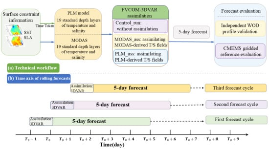
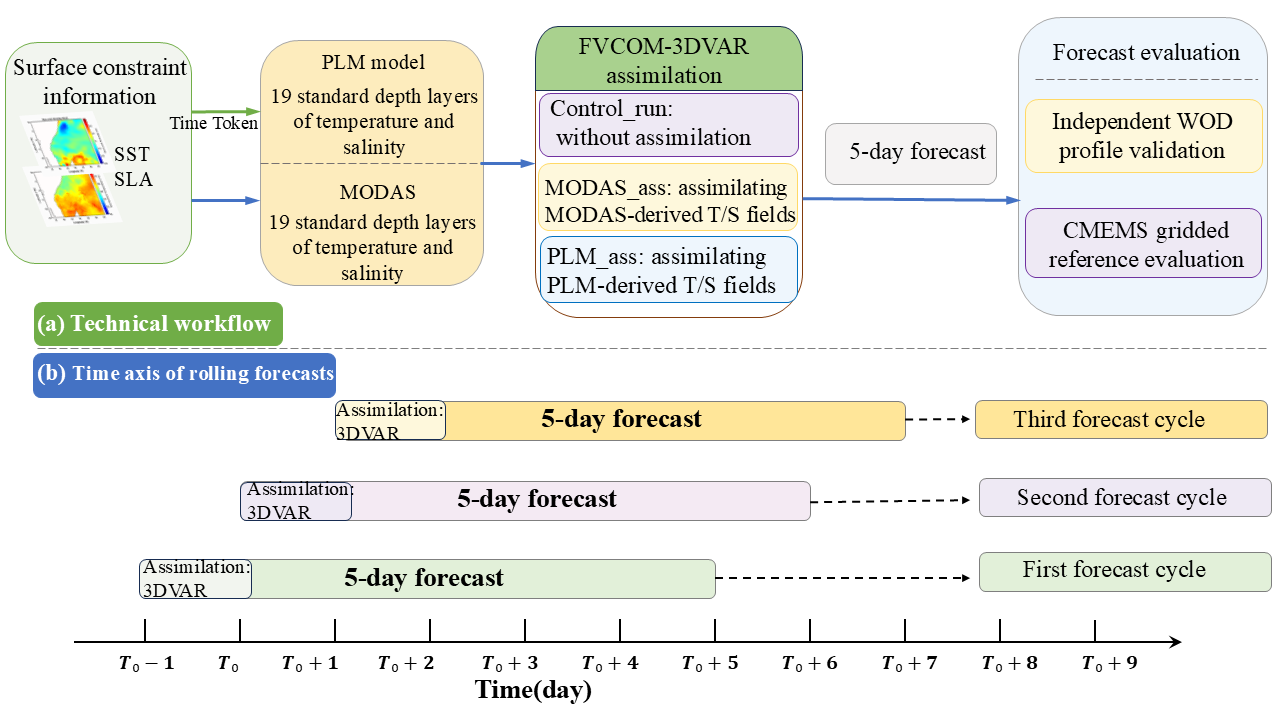
To evaluate the impact of different three-dimensional thermohaline data sources on short-term forecasts, three comparative experiments were designed: a non-assimilation control experiment (Control_run), a MODAS thermohaline field assimilation experiment (MODAS_ass), and a PLM thermohaline field assimilation experiment (PLM_ass). To clarify the relationship among pseudo-observation generation, FVCOM–3DVAR assimilation, rolling forecasts, and validation, the overall workflow is summarized in Figure 3. The corresponding experimental configurations are listed in Table 1.
Figure 3.
Technical workflow and rolling forecast design for assimilating reconstructed thermohaline fields into FVCOM–3DVAR: (a) assimilation workflow and forecast validation; (b) time axis of the 5-day rolling forecast experiments.
Table 1.
Configuration of Control_run, MODAS_ass, and PLM_ass experiments.
The forecast experiments used February, May, August, and November 2021 as representative months for different seasons. For each representative month, forecasts were initialized on Days 1–5, with one rolling forecast conducted each day. Thus, a total of 20 forecast cycles were evaluated for each experiment, corresponding to 100 forecast days over the four representative months. For MODAS_ass and PLM_ass, the forecast field from the previous day was used as the background field. The corresponding daily three-dimensional thermohaline field was assimilated at the analysis time to generate the temperature and salinity analysis fields, which were then used as the initial condition for a 5-day forecast. Control_run did not assimilate temperature or salinity and was produced directly through model integration. Forecast outputs within the 5-day range were used for the lead-time-dependent RMSE evaluation at a 6 h interval, while the Day 3 fields used for spatial error diagnostics were obtained by averaging all 6-hourly outputs within the third forecast day.
WOD profiles were used for independent station-based verification. Only WOD profiles located within the validation domain were selected, and they were matched to forecasts with the corresponding observation date and forecast lead time. Horizontally, FVCOM forecast fields were interpolated to the locations of WOD profiles. Vertically, both observations and forecasts were interpolated onto the same standard depth levels, and errors were calculated only at levels where both observation and forecast values were valid. This same-day matching strategy reduces temporal representativeness errors associated with cross-day matching. CMEMS three-dimensional thermohaline fields were used for gridded evaluation. For each initialization date, forecast lead time, and standard depth, FVCOM forecasts and CMEMS reference fields were placed on comparable spatial grids, and regional mean errors were calculated over valid ocean grid points. Because CMEMS was also used for the model initial and open-boundary conditions, these results mainly represent the consistency between the forecast fields and the reanalysis reference fields and should not be regarded as fully independent verification [43].
2.4. Evaluation Metrics
This study mainly used root-mean-square error (RMSE) to evaluate temperature and salinity forecasts from the three experiments. RMSE measures the overall deviation between forecasts and reference values and is defined as:
where denotes the forecast value at the -th valid sample, represents the corresponding reference value, and indicates the total number of valid samples used in the RMSE calculation. A smaller RMSE indicates closer agreement between the forecast and the reference. Compared with mean bias, RMSE is more sensitive to locally large errors and is therefore suitable for comparing the overall forecast error among different experiments.
In addition to RMSE, the Pearson correlation coefficient (r) was calculated to evaluate the linear consistency between the forecast and reference values. It is defined as:
where and denote the forecast and reference values at the -th valid sample, respectively, and is the number of valid forecast–reference pairs. The same valid samples used for RMSE calculation were also used for the correlation analysis. A higher correlation coefficient indicates better agreement in the variability between the forecast and reference fields.
To characterize the spatial forecast error difference between PLM_ass and Control_run, the absolute error difference was further calculated:
where represents temperature or salinity, and are the forecast results from PLM_ass and Control_run, respectively, and is the CMEMS reference field. A value smaller than 0 indicates that PLM_ass reduces the absolute forecast error relative to Control_run, whereas a value greater than 0 indicates a local increase in error. This metric was mainly used to analyze the spatial distribution of Day 3 forecast error differences in representative seasons and at selected depths.
3. Results
3.1. Forecast Verification Using Independent WOD Profiles
To evaluate the forecast skill of the three experiments at independent in situ profile locations, the temperature and salinity forecasts from Control_run, MODAS_ass, and PLM_ass were interpolated to WOD profile locations, and RMSE was calculated at the same standard depth levels. Temperature and salinity were verified separately to avoid ambiguity caused by differences in error magnitude and vertical structure between the two variables. The WOD validation involved 43 matched profile records during the four representative periods, with eight, 15, 11, and nine records in February, May, August, and November 2021, respectively. These records corresponded to 22 unique observation locations within the model domain, because some locations were sampled repeatedly during the validation periods. Therefore, the WOD-based verification was used as independent pointwise validation rather than spatially uniform regional sampling.
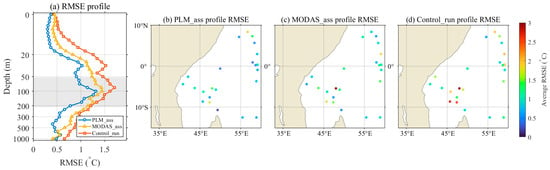
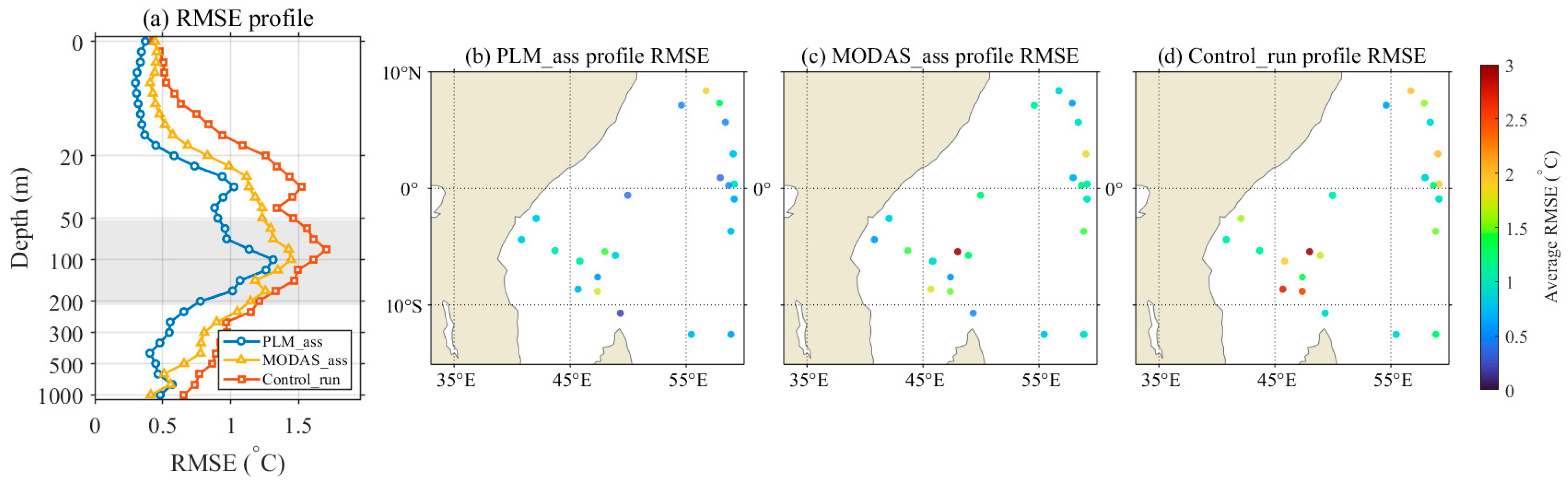
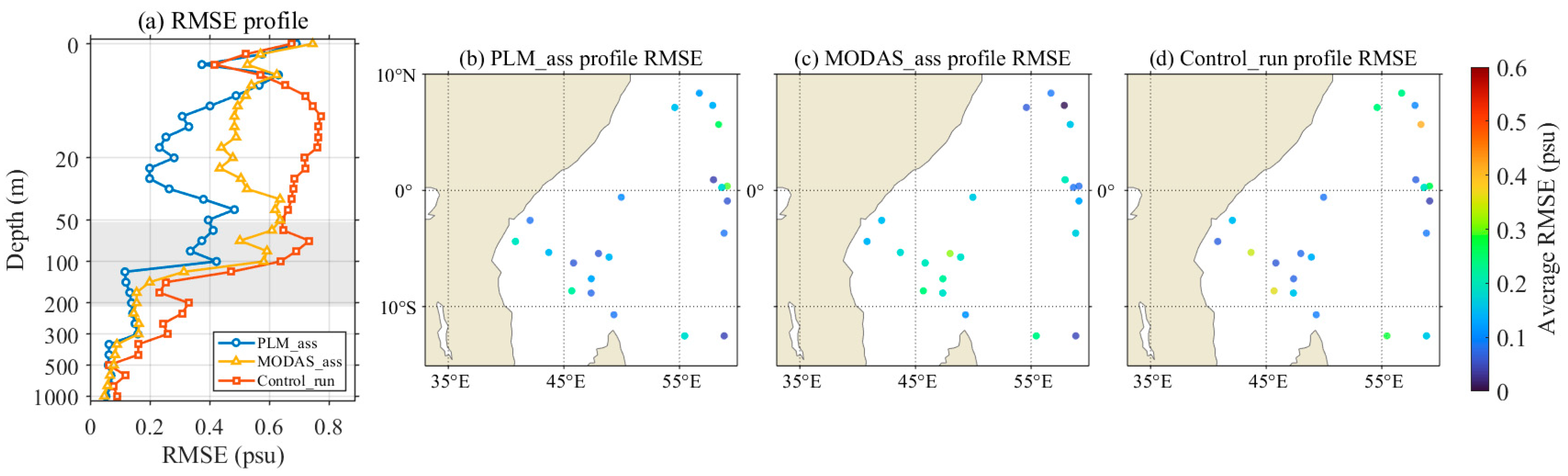
The WOD-based temperature verification results are summarized in Figure 4. The temperature verification results show that the temperature RMSE of all three experiments had a clear vertical structure. Errors were mainly concentrated in the upper ocean to the thermocline layer, especially within approximately 50–200 m, whereas errors generally decreased below 300 m. Compared with Control_run and MODAS_ass, the RMSE reduction in PLM_ass mainly occurred within 50–200 m. This indicates that PLM_ass produced lower temperature forecast errors near the thermocline. MODAS_ass also improved relative to Control_run, but its overall improvement was weaker than that of PLM_ass.
Figure 4.
Temperature forecast RMSE validation against independent WOD profiles. (a) Vertical profiles of temperature RMSE for PLM_ass, MODAS_ass, and Control_run; (b) spatial distribution of profile-averaged temperature RMSE for PLM_ass; (c) spatial distribution of profile-averaged temperature RMSE for MODAS_ass; (d) spatial distribution of profile-averaged temperature RMSE for Control_run.
The spatial distribution of temperature RMSE shows large differences among WOD profile locations, indicating strong spatial heterogeneity in temperature forecast errors over the Western Indian Ocean. Some profile locations in Control_run showed relatively high RMSE. Both MODAS_ass and PLM_ass reduced local errors to some extent, and PLM_ass reduced the error magnitude at several high-RMSE stations. However, because WOD profiles are unevenly distributed in space, local high-error points should not be directly interpreted as persistent regional error centers.
The corresponding WOD-based salinity verification results are presented in Figure 5. The salinity verification results also show a clear depth dependence, but the error reduction was weaker than that for temperature. Salinity errors were mainly concentrated in the surface to upper-thermocline layer, with relatively large errors within approximately 0–100 m. Errors decreased rapidly below 200 m, and errors at 500 m and deeper levels were relatively small. PLM_ass showed lower RMSE at some upper-ocean and subsurface depths, indicating that the PLM-reconstructed salinity field provided additional constraints for the assimilation system. Compared with temperature, however, salinity error reduction showed stronger depth dependence, and the magnitude of the reduction varied more among depth levels.
Figure 5.
Salinity forecast RMSE validation against independent WOD profiles. (a) Vertical profiles of salinity RMSE for PLM_ass, MODAS_ass, and Control_run; (b) spatial distribution of profile-averaged salinity RMSE for PLM_ass; (c) spatial distribution of profile-averaged salinity RMSE for MODAS_ass; (d) spatial distribution of profile-averaged salinity RMSE for Control_run.
Pearson correlation coefficients were further calculated using the same matched WOD forecast–observation pairs as those used for RMSE calculation. Because the WOD profiles are unevenly distributed in space and time, the correlation coefficient was used here as a supplementary pointwise measure of forecast–observation consistency rather than as a spatial field correlation. The correlations were calculated in the main improvement layers, namely, 50–200 m for temperature and 0–100 m for salinity. As summarized in Table 2, the temperature correlation increased from 0.72 in Control_run to 0.83 in MODAS_ass and 0.86 in PLM_ass, while the salinity correlation increased from 0.81 to 0.85 and 0.90, respectively. These results are consistent with the RMSE-based evaluation and suggest that PLM_ass improved the agreement with independent WOD profiles in terms of both error magnitude and pointwise variability.
Table 2.
Pearson correlation coefficients between forecasts and WOD profile observations in the main improvement layers.
The spatial distribution of salinity RMSE was more scattered than that of temperature RMSE, indicating stronger local variability in salinity forecast error reduction. PLM_ass reduced salinity errors at some profile locations, but local high-error stations remained, suggesting clear regional differences in salinity error reduction. Overall, the WOD profile verification shows that PLM_ass produced lower RMSEs and higher correlation coefficients than Control_run and MODAS_ass in the main improvement layers. Temperature error reduction was mainly concentrated within the 50–200 m thermocline and adjacent layers, whereas salinity error reduction mainly occurred from the surface to the upper thermocline.
3.2. Lead-Time and Depth Dependence of Forecast Errors
To examine how forecast errors varied with lead time and depth, RMSE values for temperature and salinity were compared among Control_run, MODAS_ass, and PLM_ass at representative depths. Overall, the RMSE of all three experiments increased with forecast lead time, indicating the accumulation of thermohaline forecast errors during short-term model integration. Compared with Control_run and MODAS_ass, PLM_ass maintained lower RMSE at all lead times, indicating lower short-term thermohaline forecast errors under the present configuration.
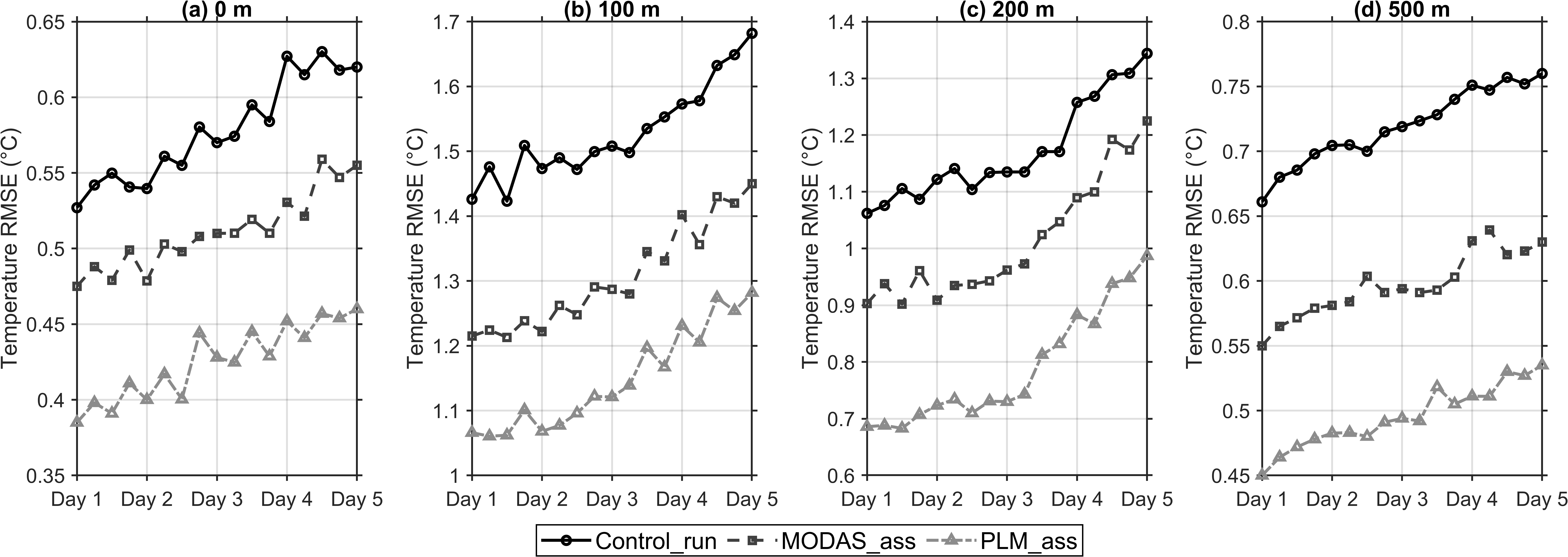
Figure 6 presents the lead-time-dependent temperature RMSE of the three experiments at representative depths. This comparison was used to assess whether the error reduction associated with PLM_ass persisted during the 5-day forecast period. Temperature RMSE showed a clear vertical dependence. Errors were relatively small at 0 and 500 m, whereas they increased substantially at 100 and 200 m. This indicates that the thermocline and its adjacent layers were the main depth range where temperature forecast errors were concentrated. Within 100–200 m, the mean temperature RMSE values of Control_run, MODAS_ass, and PLM_ass were 1.36 °C, 1.17 °C, and 0.98 °C, respectively. Compared with Control_run, PLM_ass reduced temperature RMSE by 28.0%. It further reduced RMSE by 16.6% relative to MODAS_ass. As the forecast lead time increased from Day 1 to Day 5, temperature RMSE increased in all three experiments, but PLM_ass consistently maintained the lowest error level. This indicates a relatively persistent temperature error reduction within the 5-day forecast range.
Figure 6.
Lead-time dependence of temperature forecast RMSE at different depths. Temperature RMSE variations of Control_run, MODAS_ass, and PLM_ass from Day 1 to Day 5 at (a) 0 m, (b) 100 m, (c) 200 m, and (d) 500 m.
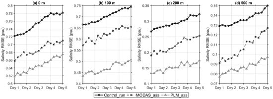
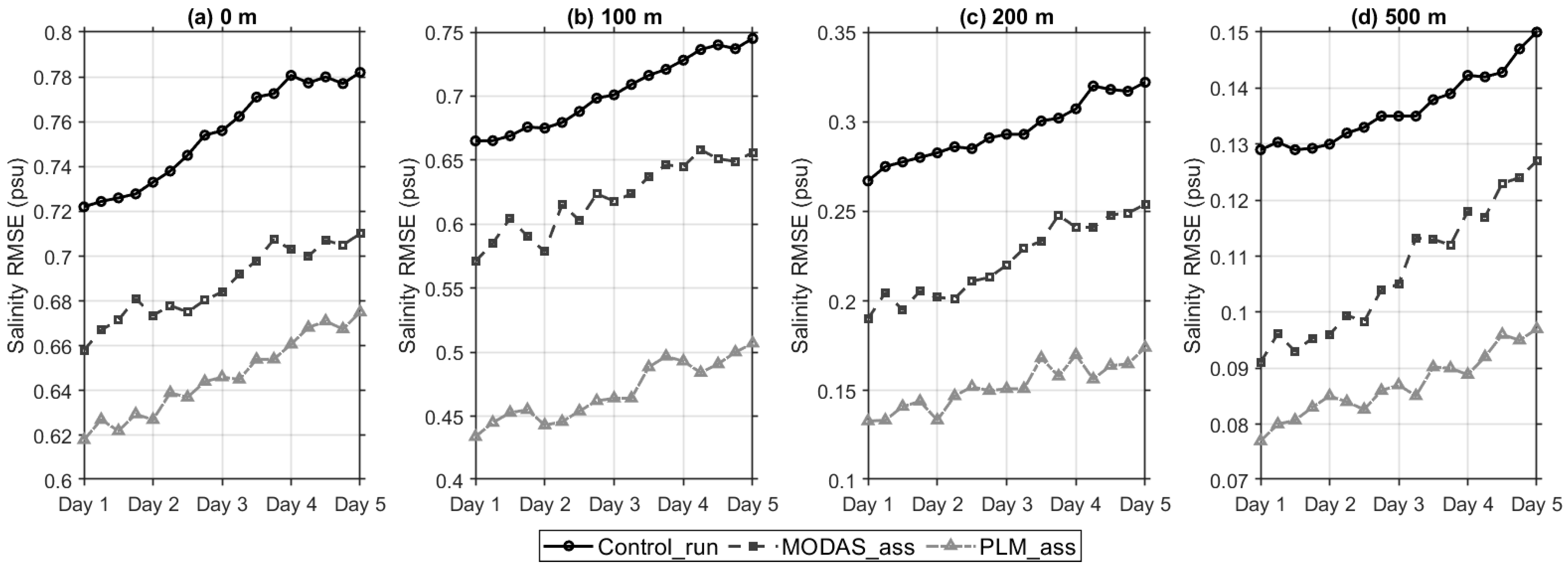
Figure 7 presents the corresponding salinity RMSE evolution with forecast lead time at the same representative depths, allowing a direct comparison with the temperature results. Salinity RMSE also increased with forecast lead time, but its vertical structure differed from that of temperature. Salinity errors were mainly concentrated near the surface and at 100 m. Errors decreased substantially below 200 m, and the 500 m layer showed the lowest overall error level. Within 0–100 m, the mean salinity RMSE values of Control_run, MODAS_ass, and PLM_ass were 0.73 psu, 0.65 psu, and 0.56 psu, respectively. Compared with Control_run, PLM_ass reduced salinity RMSE by 23.5%. It further reduced RMSE by 14.2% relative to MODAS_ass. This indicates that salinity error reduction in PLM_ass was mainly concentrated in the surface to upper-thermocline layer. Although salinity errors in deeper layers were also reduced, their absolute error magnitude was small, and this should not be overinterpreted as a substantial improvement in deep salinity structure.
Figure 7.
Lead-time dependence of salinity forecast RMSE at different depths. Salinity RMSE variations of Control_run, MODAS_ass, and PLM_ass from Day 1 to Day 5 at (a) 0 m, (b) 100 m, (c) 200 m, and (d) 500 m.
In summary, PLM_ass produced lower temperature and salinity RMSEs than the other experiments at the evaluated forecast lead times and representative depths. Temperature error reduction was mainly concentrated near the 100–200 m thermocline layer, whereas salinity error reduction was mainly found in the 0–100 m surface to upper-thermocline layer, with relatively limited differences at greater depths.
3.3. Spatial Characteristics of Forecast Error Differences
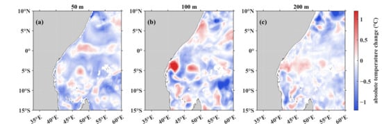
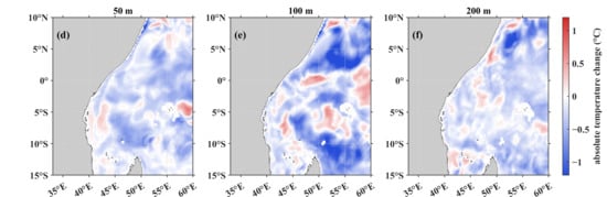
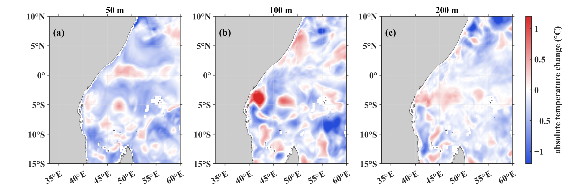
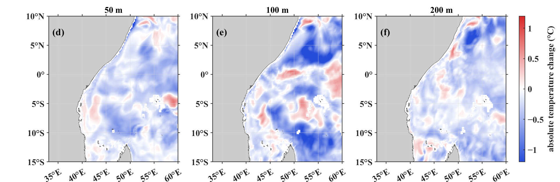
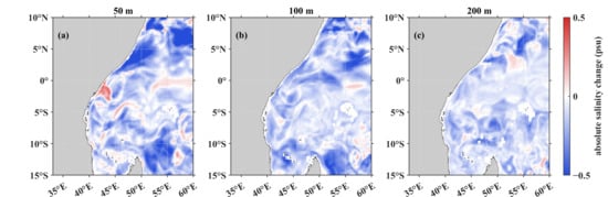
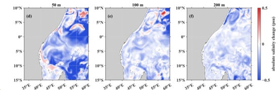
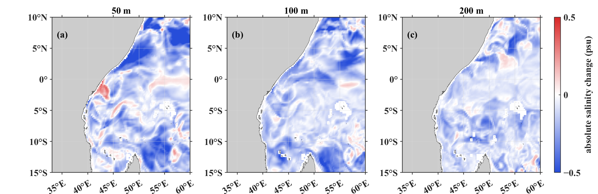
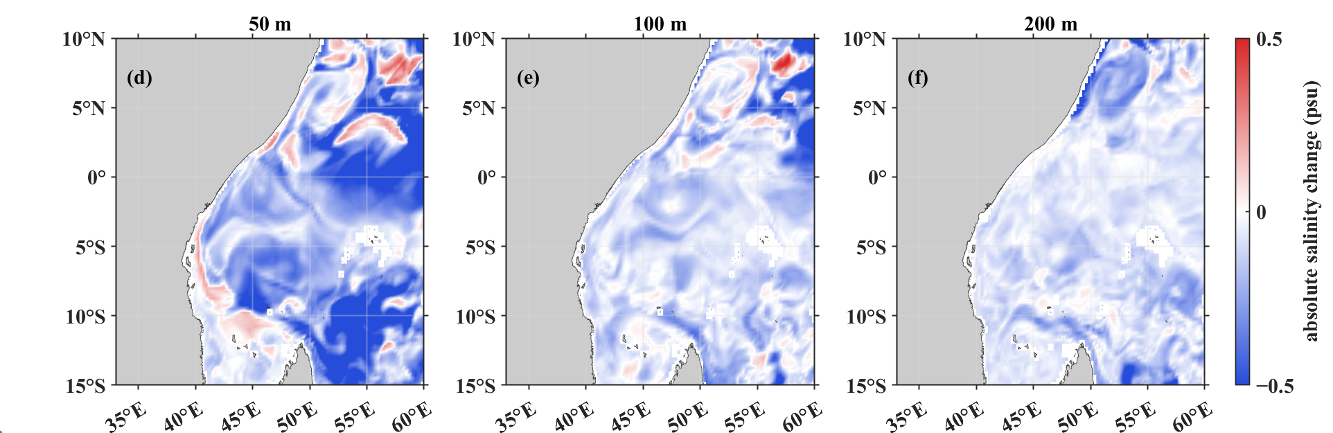
Based on the absolute error difference defined in Section 2.4, representative Day 3 seasonal cases were selected to analyze spatial forecast error differences between PLM_ass and Control_run. The temperature cases were 3 February and 3 August, which were used to compare thermocline thermal structure differences under the northeast and southwest monsoon backgrounds. The salinity cases were 3 May and 3 November, which were used to describe the spatial characteristics of upper-ocean salinity error differences during seasonal transition periods. All cases were evaluated at 50, 100, and 200 m, which are relevant to the upper ocean and thermocline. Negative values indicate lower errors in PLM_ass, whereas positive values indicate local error increases. Because these spatial diagnostics were calculated against CMEMS gridded reference fields, Figure 8 and Figure 9 should be interpreted as gridded consistency diagnostics rather than independent in situ validation. To examine the spatial structure of temperature error changes, Figure 8 presents the corresponding Day 3 absolute error differences for the temperature cases.
Figure 8.
Spatial distribution of Day 3 absolute temperature error difference between PLM_ass and Control_run on 3 February and 3 August. Panels (a–c) show the results on 3 February at 50, 100, and 200 m, respectively; panels (d–f) show the results on 3 August at 50, 100, and 200 m, respectively.
Figure 9.
Spatial distribution of Day 3 absolute salinity error difference between PLM_ass and Control_run on 3 May and 3 November. Panels (a–c) show the results on 3 May at 50, 100, and 200 m, respectively; panels (d–f) show the results on 3 November at 50, 100, and 200 m, respectively.
The absolute temperature error differences on 3 February and 3 August both showed clear spatial heterogeneity and depth dependence in the Day 3 forecasts. At 50 and 100 m, negative values dominated large parts of the study region, indicating that PLM_ass generally reduced temperature forecast errors from the upper ocean to the thermocline. The negative-value areas were more spatially continuous at 100 m, especially south of the equator, in the central part of the domain, and in the eastern part of the study region. In contrast, the magnitude of error reduction weakened at 200 m. Local negative-value regions still appeared near the northern coast and in parts of the central domain, but their spatial continuity was weaker than that at 100 m.
The temperature error differences also varied between February and August. In August, negative-value regions at 50–100 m were relatively more continuous, and local spatial gradients were more pronounced. At the same time, positive-value regions appeared in both months. These regions were mainly located near the coast, around islands, and in areas with strong local spatial gradients. This indicates that the reduction in temperature absolute error by PLM_ass had clear spatial heterogeneity.
Figure 9 presents the corresponding salinity cases using the same diagnostic metric and depth levels. The salinity error differences showed clear spatial variability in the Day 3 forecasts. At 50 and 100 m, PLM_ass produced negative values in some regions, indicating that it reduced upper-ocean salinity forecast errors to some extent. However, the positive and negative values were more interspersed than those of temperature, suggesting stronger local variability in salinity forecast error reduction. Compared with temperature, the salinity error differences showed weaker spatial continuity. This may be related to the combined influence of water mass transport, vertical mixing, and surface freshwater fluxes on the salinity field [24,54,55,56]. At 200 m, the salinity error differences were generally close to zero, with only weak positive and negative anomalies in local regions. This indicates that salinity RMSE reduction in PLM_ass was mainly concentrated in the upper ocean to the upper thermocline, with limited extension to deeper layers.
Overall, the Day 3 spatial error differences show that temperature error reduction in PLM_ass was more consistent than salinity error reduction and was mainly concentrated within 50–200 m, especially near 100 m. Salinity error reduction was more localized and weakened with increasing depth. This result is consistent with the WOD profile verification and the lead-time–depth RMSE statistics, indicating that the error reduction in PLM_ass mainly occurred from the upper ocean to the thermocline and that this feature was more evident in temperature than in salinity.
4. Discussion
The assimilation of PLM-reconstructed three-dimensional thermohaline fields into FVCOM–3DVAR reduced short-term temperature and salinity forecast errors in the Western Indian Ocean under the present experimental configuration. This reduction, however, was not spatially or vertically uniform. The forecast impact showed clear dependence on variable type, depth range, and regional dynamical setting. Compared with Control_run and MODAS_ass, PLM_ass produced a more coherent reduction in temperature errors than in salinity errors, with the most pronounced improvement occurring from the upper ocean to the thermocline. This suggests that the main contribution of PLM_ass was not a systematic correction of the entire three-dimensional thermohaline field but an improvement in those layers where the initial thermal structure exerts a strong control on short-term forecast evolution.
The largest temperature error reduction occurred within approximately 50–200 m, particularly near 100 and 200 m. This depth interval is generally associated with the upper thermocline and its adjacent layers in the Western Indian Ocean, where vertical temperature gradients are relatively strong and seasonal stratification changes are prominent [24,25,27]. In such layers, a small vertical displacement of the thermocline or an inaccurate representation of upper-ocean stratification can lead to substantial temperature errors at fixed depth levels. The reduced RMSE in PLM_ass therefore indicates that the assimilated PLM-reconstructed temperature field provided useful constraints on the initial thermal structure. The persistence of this advantage from Day 1 to Day 5 further implies that the initial thermohaline correction introduced by PLM_ass had a sustained, although not uniform, influence during short-term model integration.
The increase in RMSE with forecast lead time in all experiments indicates that forecast errors were not controlled by the initial thermohaline condition alone. After initialization, the forecast fields were also affected by atmospheric forcing uncertainty, open-boundary forcing, numerical diffusion, vertical mixing parameterization, and unresolved or insufficiently constrained mesoscale variability [1,3,57]. These error sources can progressively modify the temperature and salinity fields during the 5-day integration. Consequently, the limited spatial extent of the PLM_ass advantage should not be interpreted only as a deficiency of the reconstructed fields. It also reflects the fact that improving the initial thermohaline state does not eliminate subsequent model error growth in a dynamically active marginal and open-ocean region.
The salinity response was weaker and more heterogeneous than the temperature response. This result is physically consistent with the different controls on temperature and salinity variability. Temperature in the upper ocean and thermocline is strongly linked to surface heat exchange, stratification, and thermocline depth, whereas salinity is additionally influenced by water mass transport, horizontal advection, vertical mixing, evaporation–precipitation imbalance, and regional freshwater processes [24,55,56,58,59,60]. These processes can generate more localized and discontinuous salinity structures, particularly in regions affected by monsoon-driven circulation and water mass exchange. Therefore, even when PLM-reconstructed salinity fields supplied additional information to the assimilation system, their forecast impact could be partly modified by local dynamical processes and water mass variability. The coexistence of positive and negative salinity error differences indicates that PLM_ass produced regionally dependent salinity responses rather than a spatially coherent improvement.
Another limitation concerns the role of CMEMS in both the forecasting framework and the gridded reference evaluation. In this study, CMEMS fields were used to provide the model initial and open-boundary conditions, and they were also used as gridded reference fields for spatially continuous error evaluation. Therefore, the CMEMS-based diagnostics should be interpreted as a consistency assessment relative to a reanalysis product rather than as fully independent validation. This dependence may partly favor forecast fields that remain close to the large-scale CMEMS state, especially near the open boundaries and in regions where the model solution is strongly constrained by boundary conditions. For this reason, the WOD profile verification is regarded as the primary independent validation, whereas the CMEMS-based spatial diagnostics are used mainly to describe the regional structure and continuity of forecast error differences.
The use of reconstructed thermohaline fields as pseudo-observations also introduces methodological uncertainty. PLM and MODAS fields differ fundamentally from direct Argo, CTD, or XBT measurements. Their errors may contain spatial correlation, systematic reconstruction bias, and uncertainty associated with inferring subsurface structure from surface information. In the present FVCOM–3DVAR configuration, the observation error covariance was simplified, and the possible spatially correlated errors of the reconstructed fields were not explicitly represented. The assimilation response may therefore be sensitive to the prescribed background error and observation error covariance matrices. Underestimated pseudo-observation errors may lead to excessive adjustment of the model state, whereas overestimated errors may prevent useful reconstructed information from being effectively introduced into the analysis field. Therefore, the forecast impact reported here should be interpreted under the present prescribed diagonal- configuration rather than as a result independent of the observation error specification.
The interpretation of the forecast improvement is further constrained by the prognostic variables updated in the assimilation procedure. The present assimilation updated only temperature and salinity, without directly correcting velocity, sea surface height, or the free surface. This distinction is important in the Western Indian Ocean, where monsoon forcing, boundary currents, mesoscale eddies, upwelling, and water mass transport jointly influence the evolution of the thermohaline structure. Although temperature and salinity corrections can modify density and stratification, the absence of direct dynamical variable adjustment limits the extent to which the assimilation can constrain subsequent circulation adjustment. The results should therefore be interpreted as evidence of reduced short-term temperature and salinity forecast errors, rather than as direct evidence of improved current, boundary current, or mesoscale eddy forecasts.
The comparison between PLM_ass and MODAS_ass indicates that the forecast response was not merely a consequence of assimilating any reconstructed thermohaline product [29,61,62]. MODAS_ass provided a conventional statistically reconstructed thermohaline constraint, but its error reduction was weaker than that of PLM_ass in the present experiments. This difference suggests that the effectiveness of reconstructed fields in a dynamical assimilation system depends not only on their nominal spatial coverage but also on their information content, error structure, vertical coherence, and consistency with the model background. From this perspective, the practical value of AI-reconstructed thermohaline fields cannot be evaluated solely from static reconstruction accuracy. It must be assessed through dynamical forecast experiments, lead-time-dependent verification, and spatial error diagnostics.
These considerations indicate that the forecast impact of PLM-reconstructed thermohaline fields depends on variable type, thermocline structure, regional dynamics, pseudo-observation uncertainty, and assimilation configuration. This interpretation supports a cautious use of PLM-reconstructed fields as complementary thermohaline constraints while avoiding an overextension of the results beyond the evidence provided by the present experiments.
5. Conclusions
This study evaluated whether three-dimensional thermohaline fields inferred from sea-surface information could improve short-term temperature and salinity forecasts in the Western Indian Ocean when assimilated as external thermohaline constraints in FVCOM–3DVAR. Three comparative experiments were conducted, including a non-assimilation control experiment (Control_run), a MODAS-based assimilation experiment (MODAS_ass), and a PLM-reconstructed-field assimilation experiment (PLM_ass). The forecast impact was assessed using WOD profile observations and CMEMS gridded reference fields. Under the present regional model configuration, assimilating PLM-reconstructed thermohaline fields as pseudo-observations reduced short-term thermohaline forecast errors relative to both Control_run and MODAS_ass, indicating that AI-reconstructed subsurface information can provide additional constraints for regional forecast initialization under sparse observation conditions.
The forecast improvement showed clear variable-, depth-, and region-dependent characteristics. For temperature, the most robust reduction occurred from the upper ocean to the thermocline, particularly within 100–200 m, where the mean RMSE of PLM_ass was 0.98 °C, corresponding to reductions of 28.0% and 16.6% relative to Control_run and MODAS_ass, respectively. The lower temperature RMSE was generally maintained throughout the 5-day forecasts, suggesting that the PLM-reconstructed fields improved the initial upper-ocean and thermocline thermal structure and that this correction had a persistent influence during short-term integration. For salinity, PLM_ass also reduced forecast errors, but the response was weaker and more spatially heterogeneous. Within 0–100 m, the mean salinity RMSE of PLM_ass was 0.56 psu, representing reductions of 23.5% and 14.2% relative to Control_run and MODAS_ass, respectively, whereas the differences among the three experiments weakened below 200 m. Spatial absolute error diagnostics further showed that temperature error reduction was mainly concentrated at 50–100 m, while salinity error reduction was more localized and accompanied by local error increases in some regions.
These results suggest that PLM-reconstructed thermohaline fields can serve as supplementary pseudo-observational constraints for regional short-term thermohaline forecasting, especially for improving upper-ocean and thermocline temperature initialization. However, the forecast benefit should not be interpreted as a uniform improvement of the full three-dimensional ocean state. The assimilated reconstructed fields are not equivalent to direct in situ profiles, and the present assimilation updated only temperature and salinity rather than the full dynamical state. Future work should extend the evaluation to multi-year experiments, incorporate more independent profile observations, optimize background and observation error covariance specifications, and explore multivariate assimilation schemes that jointly adjust thermohaline and dynamical variables.
Author Contributions
Conceptualization, Q.Y. and D.Z.; methodology, Q.Y., J.W. and X.Z.; validation, Q.Y., X.Z. and D.Z.; writing—original draft preparation, Q.Y. and D.Z.; writing—review and editing, Q.Y., R.X. and D.Z. All authors have read and agreed to the published version of the manuscript.
Funding
This research was funded by the Hainan Province Science and Technology Special Fund (No. SOLZSKY2025007), the Key Research and Development Program sponsored by the Ministry of Science and Technology (MOST) 2023YFC3107701 and 2023YFC3107901, and the National Natural Science Foundation of China (No. 42375143).
Data Availability Statement
The publicly available datasets used in this study are described in the Acknowledgments Section. The processed data and analysis scripts are available from the corresponding author upon reasonable request.
Acknowledgments
The GLORYS12V1 global ocean physical reanalysis used in this study is available from the Copernicus Marine Service at https://data.marine.copernicus.eu/product/GLOBAL_MULTIYEAR_PHY_001_030/description, accessed on 31 December 2025. The World Ocean Database used for independent validation is available from NOAA National Centers for Environmental Information at https://www.ncei.noaa.gov/products/world-ocean-database, accessed on 31 December 2025, and data access is provided through https://www.ncei.noaa.gov/access/world-ocean-database-select/dbsearch.html, accessed on 31 December 2025. The authors thank these institutions and programs for providing open access to the datasets used in this study.
Conflicts of Interest
The authors declare no conflicts of interest.
Abbreviations
The following abbreviations are used in this manuscript:
| FVCOM | Finite Volume Community Ocean Model |
| 3DVAR | three-dimensional variational data assimilation |
| FVCOM–3DVAR | Finite Volume Community Ocean Model with three-dimensional variational data assimilation |
| MODAS | Modular Ocean Data Assimilation System |
| PLM | pretrained language model |
| WOD | World Ocean Database |
| CMEMS | Copernicus Marine Environment Monitoring Service |
| RMSE | root-mean-square error |
| CTD | conductivity–temperature–depth |
| XBT | expendable bathythermograph |
| ERA5 | fifth-generation European Centre for Medium-Range Weather Forecasts atmospheric reanalysis |
| GSHHG | Global Self-consistent, Hierarchical, High-resolution Geography Database |
| TPXO | TOPEX/Poseidon Global Inverse Solution |
| HYCOM–NCODA | HYbrid Coordinate Ocean Model–Navy Coupled Ocean Data Assimilation |
| AI | artificial intelligence |
References
- Stammer, D. Adjusting internal model errors through ocean state estimation. J. Phys. Oceanogr. 2005, 35, 1143–1153. [Google Scholar] [CrossRef] [Scilit]
- Chassignet, E.P.; Hurlburt, H.E.; Metzger, E.J.; Smedstad, O.M.; Cummings, J.A.; Halliwell, G.R.; Bleck, R.; Baraille, R.; Wallcraft, A.J.; Lozano, C.; et al. U.S. GODAE: Global ocean prediction with the HYbrid Coordinate Ocean Model (HYCOM). Oceanography 2009, 22, 64–75. [Google Scholar] [CrossRef] [Scilit]
- Martin, M.J.; Balmaseda, M.; Bertino, L.; Brasseur, P.; Brassington, G.; Cummings, J.; Fujii, Y.; Lea, D.J.; Lellouche, J.-M.; Mogensen, K.; et al. Status and future of data assimilation in operational oceanography. J. Oper. Oceanogr. 2015, 8, s28–s48. [Google Scholar] [CrossRef] [Scilit]
- Francis, P.A.; Jithin, A.K.; Effy, J.B.; Chatterjee, A.; Chakraborty, K.; Paul, A.; Balaji, B.; Shenoi, S.S.C.; Biswamoy, P.; Mukherjee, A.; et al. High-resolution operational ocean forecast and reanalysis system for the Indian Ocean. Bull. Am. Meteorol. Soc. 2020, 101, E1340–E1356. [Google Scholar] [CrossRef] [Scilit]
- Qin, Y.; Yu, Q.; Wan, L.; Liu, Y.; Mo, H.; Wang, Y.; Meng, S.; Wu, X.; Sui, D.; Xie, J. A global-ocean-data assimilation for operational oceanography. J. Mar. Sci. Eng. 2023, 11, 2255. [Google Scholar] [CrossRef] [Scilit]
- Cummings, J.A. Operational multivariate ocean data assimilation. Q. J. R. Meteorol. Soc. 2005, 131, 3583–3604. [Google Scholar] [CrossRef] [Scilit]
- Li, Z.; Chao, Y.; McWilliams, J.C.; Ide, K. A three-dimensional variational data assimilation scheme for the Regional Ocean Modeling System. J. Atmos. Ocean. Technol. 2008, 25, 2074–2090. [Google Scholar] [CrossRef] [Scilit]
- Moore, A.M.; Arango, H.G.; Broquet, G.; Powell, B.S.; Weaver, A.T.; Zavala-Garay, J. The Regional Ocean Modeling System (ROMS) 4-dimensional variational data assimilation systems. Part I: System overview and formulation. Prog. Oceanogr. 2011, 91, 34–49. [Google Scholar] [CrossRef] [Scilit]
- Ngodock, H.E.; Carrier, M.J. A 4DVAR system for the Navy Coastal Ocean Model. Part I: System description and assimilation of synthetic observations in Monterey Bay. Mon. Weather. Rev. 2014, 142, 2085–2107. [Google Scholar] [CrossRef] [Scilit]
- Altaf, M.U.; Butler, T.; Mayo, T.; Luo, X.; Dawson, C.; Heemink, A.W.; Hoteit, I. A comparison of ensemble Kalman filters for storm surge assimilation. Mon. Weather Rev. 2014, 142, 2899–2914. [Google Scholar] [CrossRef] [Scilit]
- Pringle, W.J.; Wirasaet, D.; Roberts, K.J.; Westerink, J.J. Global storm tide modeling with ADCIRC v55: Unstructured mesh design and performance. Geosci. Model Dev. 2021, 14, 1125–1145. [Google Scholar] [CrossRef] [Scilit]
- Arkhipkin, V.S.; Ilyin, V.I.; Myslenkov, S.A.; Pishchalnik, V.M.; Latkovskaya, E.M.; Shumilov, I.V.; Romanyuk, V.A.; Pishchalnik, A.V. Modeling of tides in the La Perouse Strait using a high-resolution grid. Oceanology 2026, 66, 385–397. [Google Scholar] [CrossRef] [Scilit]
- Bannister, R.N. A review of forecast error covariance statistics in atmospheric variational data assimilation. I: Characteristics and measurements of forecast error covariances. Q. J. R. Meteorol. Soc. 2008, 134, 1951–1970. [Google Scholar] [CrossRef] [Scilit]
- Donlon, C.J.; Martin, M.; Stark, J.; Roberts-Jones, J.; Fiedler, E.; Wimmer, W. The Operational Sea Surface Temperature and Sea Ice Analysis (OSTIA) system. Remote Sens. Environ. 2012, 116, 140–158. [Google Scholar] [CrossRef] [Scilit]
- Taburet, G.; Sanchez-Roman, A.; Ballarotta, M.; Pujol, M.-I.; Legeais, J.-F.; Fournier, F.; Faugère, Y.; Dibarboure, G. DUACS DT2018: 25 years of reprocessed sea level altimetry products. Ocean Sci. 2019, 15, 1207–1224. [Google Scholar] [CrossRef] [Scilit]
- Roemmich, D.; Johnson, G.C.; Riser, S.; Davis, R.; Gilson, J.; Owens, W.B.; Garzoli, S.; Schmid, C.; Ignaszewski, M. The Argo Program: Observing the global oceans with profiling floats. Oceanography 2009, 22, 34–43. [Google Scholar] [CrossRef] [Scilit]
- Wong, A.P.S.; Wijffels, S.E.; Riser, S.C.; Pouliquen, S.; Hosoda, S.; Roemmich, D.; Gilson, J.; Johnson, G.C.; Martini, K.; Murphy, D.J.; et al. Argo data 1999–2019: Two million temperature–salinity profiles and subsurface velocity observations from a global array of profiling floats. Front. Mar. Sci. 2020, 7, 700. [Google Scholar] [CrossRef] [Scilit]
- Boyer, T.P.; Baranova, O.K.; Coleman, C.; Garcia, H.E.; Grodsky, A.; Locarnini, R.A.; Mishonov, A.V.; Paver, C.R.; Reagan, J.R.; Seidov, D.; et al. World Ocean Database 2018; NOAA Atlas NESDIS 87; NOAA National Centers for Environmental Information: Silver Spring, MD, USA, 2018. [Google Scholar]
- Gwyther, D.E.; Kerry, C.; Roughan, M.; Keating, S.R. Observing system simulation experiments reveal that subsurface temperature observations improve estimates of circulation and heat content in a dynamic western boundary current. Geosci. Model Dev. 2022, 15, 6541–6565. [Google Scholar] [CrossRef] [Scilit]
- Schott, F.A.; McCreary, J.P. The monsoon circulation of the Indian Ocean. Prog. Oceanogr. 2001, 51, 1–123. [Google Scholar] [CrossRef] [Scilit]
- Shankar, D.; Vinayachandran, P.N.; Unnikrishnan, A.S. The monsoon currents in the north Indian Ocean. Prog. Oceanogr. 2002, 52, 63–120. [Google Scholar] [CrossRef] [Scilit]
- Zang, N.; Sprintall, J.; Ienny, R.; Wang, F. Seasonality of the Somali Current/Undercurrent system. Deep Sea Res. Part II Top. Stud. Oceanogr. 2021, 191–192, 104953. [Google Scholar] [CrossRef] [Scilit]
- Beal, L.M.; Donohue, K.A. The Great Whirl: Observations of its seasonal development and interannual variability. J. Geophys. Res. Ocean. 2013, 118, 1–13. [Google Scholar] [CrossRef] [Scilit]
- Phillips, H.E.; Tandon, A.; Furue, R.; Hood, R.; Ummenhofer, C.C.; Benthuysen, J.A.; Menezes, V.; Hu, S.; Webber, B.; Sanchez-Franks, A.; et al. Progress in understanding of Indian Ocean circulation, variability, air–sea exchange, and impacts on biogeochemistry. Ocean Sci. 2021, 17, 1677–1751. [Google Scholar] [CrossRef] [Scilit]
- Hermes, J.C.; Reason, C.J.C. Annual cycle of the South Indian Ocean (Seychelles–Chagos) Thermocline Ridge in a regional ocean model. J. Geophys. Res. Ocean. 2008, 113, C04035. [Google Scholar] [CrossRef] [Scilit]
- Swart, N.C.; Lutjeharms, J.R.E.; Ridderinkhof, H.; de Ruijter, W.P.M. Observed characteristics of Mozambique Channel eddies. J. Geophys. Res. Ocean. 2010, 115, C09006. [Google Scholar] [CrossRef] [Scilit]
- Mubarrok, S.; Azminuddin, F.; Jang, C.J. Assessment of thermocline depth bias in the Seychelles–Chagos Thermocline Ridge of the southwestern Indian Ocean simulated by the CMIP6 models. Front. Mar. Sci. 2023, 10, 1239885. [Google Scholar] [CrossRef] [Scilit]
- Hermes, J.C.; Masumoto, Y.; Beal, L.M.; Roxy, M.K.; Vialard, J.; Andres, M.; Annamalai, H.; Behera, S.; D’Adamo, N.; Doi, T.; et al. A sustained ocean observing system in the Indian Ocean for climate related scientific knowledge and societal needs. Front. Mar. Sci. 2019, 6, 355. [Google Scholar] [CrossRef] [Scilit]
- Fox, D.N.; Teague, W.J.; Barron, C.N.; Carnes, M.R.; Lee, C.M. The Modular Ocean Data Assimilation System (MODAS). J. Atmos. Ocean. Technol. 2002, 19, 240–252. [Google Scholar]
- Guinehut, S.; Le Traon, P.-Y.; Larnicol, G.; Philipps, S. Combining Argo and remote-sensing data to estimate the ocean three-dimensional temperature fields: A first approach based on simulated observations. J. Mar. Syst. 2004, 46, 85–98. [Google Scholar] [CrossRef] [Scilit]
- Meng, L.; Yan, C.; Zhuang, W.; Zhang, W.; Yan, X.-H. Reconstruction of three-dimensional temperature and salinity fields from satellite observations. J. Geophys. Res. Ocean. 2021, 126, e2021JC017605. [Google Scholar] [CrossRef] [Scilit]
- Su, H.; Yang, X.; Lu, W.; Yan, X.-H. Estimating subsurface thermohaline structure of the global ocean using surface remote sensing observations. Remote Sens. 2019, 11, 1598. [Google Scholar] [CrossRef] [Scilit]
- Su, H.; Wang, A.; Zhang, T.; Qin, T.; Du, X.; Yan, X.-H. Super-resolution of subsurface temperature field from remote sensing observations based on machine learning. Int. J. Appl. Earth Obs. Geoinf. 2021, 102, 102440. [Google Scholar] [CrossRef] [Scilit]
- Pauthenet, E.; Bachelot, L.; Balem, K.; Maze, G.; Tréguier, A.-M.; Roquet, F.; Fablet, R.; Tandeo, P. Four-dimensional temperature, salinity and mixed-layer depth in the Gulf Stream, reconstructed from remote-sensing and in situ observations with neural networks. Ocean Sci. 2022, 18, 1221–1244. [Google Scholar] [CrossRef] [Scilit]
- Smith, P.A.H.; Sørensen, K.A.; Buongiorno Nardelli, B.; Chauhan, A.; Christensen, A.; St. John, M.; Rodrigues, F.; Mariani, P. Reconstruction of subsurface ocean state variables using convolutional neural networks with combined satellite and in situ data. Front. Mar. Sci. 2023, 10, 1218514. [Google Scholar] [CrossRef] [Scilit]
- Song, T.; Wei, W.; Meng, F.; Wang, J.; Han, R.; Xu, D. Inversion of ocean subsurface temperature and salinity fields based on spatio-temporal correlation. Remote Sens. 2022, 14, 2587. [Google Scholar] [CrossRef] [Scilit]
- Mao, K.; Liu, C.; Zhang, S.; Gao, F. Reconstructing ocean subsurface temperature and salinity from sea surface information based on dual path convolutional neural networks. J. Mar. Sci. Eng. 2023, 11, 1030. [Google Scholar] [CrossRef] [Scilit]
- Tian, T.; Cheng, L.; Wang, G.; Abraham, J.; Wei, W.; Ren, S.; Zhu, J.; Song, J.; Leng, H. Reconstructing ocean subsurface salinity at high resolution using a machine learning approach. Earth Syst. Sci. Data 2022, 14, 5037–5060. [Google Scholar] [CrossRef] [Scilit]
- Zhang, J.; Zhang, X.; Wang, X.; Ning, P.; Zhang, A. Reconstructing 3D ocean subsurface salinity from T–S mapping via a data-driven deep learning model. Ocean Model. 2023, 184, 102232. [Google Scholar] [CrossRef] [Scilit]
- Song, T.; Xu, G.; Yang, K.; Li, X.; Peng, S. Convformer: A model for reconstructing ocean subsurface temperature and salinity fields based on multi-source remote sensing observations. Remote Sens. 2024, 16, 2422. [Google Scholar] [CrossRef] [Scilit]
- Xie, H.; Xu, Q.; Cheng, Y.; Yin, X.; Fan, K. Reconstructing three-dimensional salinity field of the South China Sea from satellite observations. Front. Mar. Sci. 2023, 10, 1168486. [Google Scholar] [CrossRef] [Scilit]
- Desroziers, G.; Berre, L.; Chapnik, B.; Poli, P. Diagnosis of observation, background and analysis-error statistics in observation space. Q. J. R. Meteorol. Soc. 2005, 131, 3385–3396. [Google Scholar] [CrossRef] [Scilit]
- Lellouche, J.-M.; Greiner, E.; Bourdallé-Badie, R.; Garric, G.; Melet, A.; Drévillon, M.; Bricaud, C.; Hamon, M.; Le Galloudec, O.; Regnier, C.; et al. The Copernicus Global 1/12° Oceanic and Sea Ice GLORYS12 reanalysis. Front. Earth Sci. 2021, 9, 698876. [Google Scholar] [CrossRef] [Scilit]
- Schott, F.A.; Xie, S.-P.; McCreary, J.P. Indian Ocean circulation and climate variability. Rev. Geophys. 2009, 47, RG1002. [Google Scholar] [CrossRef] [Scilit]
- Amante, C.; Eakins, B.W. ETOPO1 1 Arc-Minute Global Relief Model: Procedures, Data Sources and Analysis; NOAA Technical Memorandum NESDIS NGDC-24; National Geophysical Data Center, NOAA: Boulder, CO, USA, 2009. [Google Scholar] [CrossRef] [Scilit]
- Wessel, P.; Smith, W.H.F. A global, self-consistent, hierarchical, high-resolution shoreline database. J. Geophys. Res. Solid Earth 1996, 101, 8741–8743. [Google Scholar] [CrossRef] [Scilit]
- Hersbach, H.; Bell, B.; Berrisford, P.; Hirahara, S.; Horányi, A.; Muñoz-Sabater, J.; Nicolas, J.; Peubey, C.; Radu, R.; Schepers, D.; et al. The ERA5 global reanalysis. Q. J. R. Meteorol. Soc. 2020, 146, 1999–2049. [Google Scholar] [CrossRef] [Scilit]
- Egbert, G.D.; Erofeeva, S.Y. Efficient inverse modeling of barotropic ocean tides. J. Atmos. Ocean. Technol. 2002, 19, 183–204. [Google Scholar]
- Chen, C.; Beardsley, R.C.; Cowles, G. An unstructured grid, finite-volume coastal ocean model (FVCOM) system. Oceanography 2006, 19, 78–89. [Google Scholar] [CrossRef] [Scilit]
- Chen, C.; Beardsley, R.C.; Cowles, G. An Unstructured Grid, Finite-Volume Community Ocean Model: FVCOM User Manual; School for Marine Science and Technology, University of Massachusetts Dartmouth: New Bedford, MA, USA, 2013. [Google Scholar]
- Mellor, G.L.; Yamada, T. Development of a turbulence closure model for geophysical fluid problems. Rev. Geophys. 1982, 20, 851–875. [Google Scholar] [CrossRef] [Scilit]
- Lorenc, A.C. Analysis methods for numerical weather prediction. Q. J. R. Meteorol. Soc. 1986, 112, 1177–1194. [Google Scholar] [CrossRef]
- Cummings, J.A.; Smedstad, O.M. Variational data assimilation for the global ocean. In Data Assimilation for Atmospheric, Oceanic and Hydrologic Applications, Vol. II; Park, S.K., Xu, L., Eds.; Springer: Berlin/Heidelberg, Germany, 2013; pp. 303–343. [Google Scholar] [CrossRef] [Scilit]
- Boutin, J.; Chao, Y.; Asher, W.E.; Delcroix, T.; Drucker, R.; Drushka, K.; Kolodziejczyk, N.; Lee, T.; Reul, N.; Reverdin, G.; et al. Satellite and in situ salinity: Understanding near-surface stratification and subfootprint variability. Bull. Am. Meteorol. Soc. 2016, 97, 1391–1407. [Google Scholar] [CrossRef] [Scilit]
- Durack, P.J. Ocean salinity and the global water cycle. Oceanography 2015, 28, 20–31. [Google Scholar] [CrossRef] [Scilit]
- Durack, P.J.; Wijffels, S.E.; Matear, R.J. Ocean salinities reveal strong global water cycle intensification during 1950 to 2000. Science 2012, 336, 455–458. [Google Scholar] [CrossRef] [Scilit] [PubMed]
- Chao, Y.; Farrara, J.D.; Zhang, H.; Armenta, K.J.; Centurioni, L.; Chavez, F.; Girton, J.B.; Rudnick, D.; Walter, R.K. Development, implementation, and validation of a California coastal ocean modeling, data assimilation, and forecasting system. Deep Sea Res. Part II Top. Stud. Oceanogr. 2018, 151, 49–63. [Google Scholar] [CrossRef] [Scilit]
- Beal, L.M.; Ffield, A.; Gordon, A.L. Spreading of Red Sea Overflow waters in the Indian Ocean. J. Geophys. Res. Ocean. 2000, 105, 8549–8564. [Google Scholar] [CrossRef] [Scilit]
- Yu, L. A global relationship between the ocean water cycle and near-surface salinity. J. Geophys. Res. Ocean. 2011, 116, C10025. [Google Scholar] [CrossRef] [Scilit]
- Schanze, J.J.; Schmitt, R.W.; Yu, L.L. The global oceanic freshwater cycle: A state-of-the-art quantification. J. Mar. Res. 2010, 68, 569–595. [Google Scholar] [CrossRef] [Scilit]
- Guinehut, S.; Dhomps, A.-L.; Larnicol, G.; Le Traon, P.-Y. High resolution 3-D temperature and salinity fields derived from in situ and satellite observations. Ocean Sci. 2012, 8, 845–857. [Google Scholar] [CrossRef] [Scilit]
- Liu, L.; Peng, S.; Huang, R.X. Reconstruction of ocean’s interior from observed sea surface information. J. Geophys. Res. Ocean. 2017, 122, 1042–1056. [Google Scholar] [CrossRef] [Scilit]

Disclaimer/Publisher’s Note: The statements, opinions and data contained in all publications are solely those of the individual author(s) and contributor(s) and not of MDPI and/or the editor(s). MDPI and/or the editor(s) disclaim responsibility for any injury to people or property resulting from any ideas, methods, instructions or products referred to in the content. |
© 2026 by the authors. Licensee MDPI, Basel, Switzerland. This article is an open access article distributed under the terms and conditions of the Creative Commons Attribution (CC BY) license.