


Abstract
To investigate the influence of propeller rotational speed on the flooding process, sailing trajectory, and motion responses of a damaged surface naval ship under various sea conditions, numerical simulations were conducted using STAR-CCM+. The study is based on the Finite Volume Method (FVM), the Volume of Fluid (VOF) approach, the body force method, overset grids, and a multi-degree-of-freedom motion system. The flooding behavior, trajectory evolution, and hydrodynamic responses of the damaged naval ship were analyzed under calm water, head sea, and beam sea conditions, each at four distinct propeller speeds. The research findings indicate that, regardless of the sea state, a damaged naval ship initially travels in a straight line for a certain distance before transitioning into a curved trajectory. The length of the straight-line travel remains largely unaffected by variations in propeller rotational speed but varies with different sea conditions. Notably, under beam sea conditions, this distance exhibits a significant reduction. The subsequent curved motion trajectory is significantly influenced by the propeller rotational speed and varying wave directions. In calm water, the motion exhibits repetitive circular trajectories toward the damaged side, with the diameter of the circular path increasing as the propeller speed rises. Under head and beam sea conditions, the vessel exhibits a helical motion, with the trajectory becoming more pronounced as the propeller rotational speed increases. In all three wave conditions, the maximum cumulative ingress of the damaged compartment is positively correlated with the propeller speed, whereas the ship’s roll, pitch, and heave motions exhibit distinct variation trends.
1. Introduction
During modern maritime combat, vessels are highly susceptible to hull damage due to attacks from integrated multi-dimensional and multi-directional weapons in the air and sea. In actual combat scenarios, if a vessel sustains external damage resulting in flooding, and the extent of hull damage is minimal with limited flooding in the compartments, and the ship has not sunk, the vessel’s posture can be adjusted as needed to either continue engaging in combat or return to base for repairs, depending on the situation. Therefore, an in-depth study of the flooding process, changes in the vessel’s trajectory, and motion responses under different sea conditions, where the hull is damaged but the propulsion remains intact, is crucial for ensuring the navigational safety and rapid recovery of operational capability of damaged ships.
The flooding process of a damaged ship involves complex nonlinear phenomena including seawater inflow, slamming, liquid sloshing inside compartments, and fluid exchange between the interior and exterior of the hull, and the coupling interaction among the hull, incoming water, and waves significantly influences motion responses such as roll, pitch, and heave, thereby threatening navigation safety. Extensive research has been conducted in this area. Regarding the flooding process, Bian et al. investigated the effects of breach size, location, and shape on the flooding rate [1]; Ruponen et al. evaluated the survivability and flooding process of a damaged ro-ro passenger vessel in calm water and irregular waves through model tests [2]; Siddiqui et al. found that initial load conditions determine the final flooded state, breach size mainly affects roll damping, and air compressibility in enclosed compartments forms a coupled spring system with the internal water, limiting free-surface motion [3]; Liu et al. showed that different baffle arrangements significantly alter water dispersion inside the compartment, and an appropriate increase in baffle number can mitigate the impact of damage on motion characteristics [4]; Hu et al. studied the flooding process and six-degree-of-freedom motion of an unmanned barge under explosive bulkhead deformation using numerical simulation [5].
In terms of motion response and stability, Hu et al. found that the capsizing probability of a powerless damaged ship first decreases and then increases during flooding [6]; later, using the DTMB-5415 model, they observed significant differences in roll motion under wave directions of 0° and 180° [7]; Zhang et al., using STAR-CCM+, analysed the effects of ventilation level, air compressibility, symmetric/asymmetric flooding, and internal opening arrangements on the stability and motion response of a damaged ship, reporting that asymmetric flooding has a greater impact on roll motion and different opening paths lead to different flooding routes thus affecting the motion response [8,9,10]; Gao et al. investigated the variation in natural roll frequency and roll response of a ro-ro passenger vessel in intact and damaged conditions (with or without internal water) under beam seas [11,12]; Bu et al. analysed the motion response of a damaged ship in regular waves and the safety boundaries under different wave conditions, discussing the effect of roll motion on these boundaries [13,14]; a combined viscous-potential flow method was proposed to predict the flooding process and dynamic characteristics of a damaged box-shaped barge [15]; Begovic et al. studied the motion response characteristics of a non-propelled naval vessel in intact and damaged states under head, beam and oblique waves, and found that the orientation of the damage opening affects the RAO and free-drift velocity [16].
Regarding manoeuvrability of damaged ships, Luo et al., based on CFD simulations, investigated the turning manoeuvrability of an ONRT model in both damaged and intact conditions, validating the capability of CFD to predict manoeuvrability [17]; Dong et al. simulated the rotational motion of a damaged vessel under various initial heel, trim and breach closure conditions, and assessed the impact of damage on turning manoeuvrability [18]; Liu et al., using dynamic overset grid CFD technology, developed a data-driven Stacking algorithm that can efficiently and accurately predict the roll amplitude of a damaged ship [19]. Issa-Zadeh et al. combined physics-based hydrodynamic calculations with machine learning to predict fuel consumption under different propulsion scenarios, including advanced propellers, providing a valuable reference for interpreting propulsion-related hydrodynamic responses [20].
In summary, existing studies mainly focus on the flooding, stability and motion response of non-propelled or towed damaged ships, or on the manoeuvrability of intact ships. However, the coupling effect of different propeller speeds (i.e., active propulsion) and different sea conditions (calm water, head waves, beam waves) on the flooding process, trajectory and motion responses of a self-propelled damaged warship has not been systematically investigated, which is the key scientific problem that the present study aims to address. the present study investigates the coupled flooding process, navigation trajectory, and motion response of a damaged DTMB-5415 ship under calm water, head sea, and beam sea conditions at four propeller rotational speeds. The main contributions are threefold: (1) quantifying how propeller speed alters the flooding evolution; (2) clarifying its influence on trajectory transition and motion response; and (3) identifying the sea-state-dependent mechanisms governing these coupled effects.
The remainder of this paper is organized as follows: Section 2 presents the governing models and numerical methods; Section 3 describes the computational setup and study cases; Section 4 discusses the results; and Section 5 summarizes the conclusions and future work.
The present study adopts a high-fidelity CFD framework that combines the finite volume method (FVM) for spatial discretisation, the Reynolds-averaged Navier–Stokes (RANS) equations with the standard k-ε turbulence model for flow closure, the volume of fluid (VOF) method for free-surface capturing, overset grids for large-amplitude hull motions, and a six-degree-of-freedom (6-DOF) rigid-body motion solver. This framework is capable of capturing strongly nonlinear and viscous phenomena—such as wave breaking, sloshing, and flooding-hull interaction—that are typically beyond the reach of potential-flow methods or reduced-order models. Consequently, it provides the fidelity required for a systematic comparison of propeller speed effects on the trajectory, flooding process, and motion responses of a damaged ship under different sea conditions. A quantitative comparison with alternative modelling approaches is not included in this study, but it is a valuable direction for future research.
2. Mathematical Models and Numerical Methods
This section describes the mathematical and numerical framework used to simulate the flooding process, motion responses, and trajectory of the damaged ship under various sea conditions. The coordinate system is first defined. The governing equations are discretised using the finite volume method (FVM), and the free surface is captured by the volume of fluid (VOF) approach. The six-degree-of-freedom (6-DOF) rigid body equations govern the ship’s motions, while the propeller thrust is modelled using a body force method (actuator disk) to avoid the high computational cost of fully resolved geometry. Finally, the numerical method is validated against a published floating body submersion experiment.
2.1. Coordinate System Setup
During the navigation of a damaged ship, three distinct coordinate systems are defined to describe the instantaneous position and motion of the computational domain–ship–propeller system. These coordinate systems include the Earth-fixed coordinate system, the body-fixed coordinate system, and the propeller-fixed coordinate system, as illustrated in Figure 1. The origin of the Earth-fixed coordinate system is located at the intersection of the ship’s stern perpendicular, the centerline, and the design waterline. The positive direction of the x-axis points towards the bow, the positive direction of the y-axis points towards the port side, and the positive direction of the z-axis is upward. The earth-fixed coordinate system remains constant throughout the vessel’s entire voyage and is used to describe the relative position and motion of other coordinate systems. The origin of the body-fixed coordinate system is located at the ship’s center of gravity, with the initial direction of the axes aligning with those of the global coordinate system. This coordinate system moves in correspondence with the ship’s motion. The coordinate system of the propeller is fixed at the center of the propeller disk. This system is a sub-coordinate system of the body-fixed coordinate system and moves with the ship. Since the propeller only undergoes rotational motion, the coordinate system illustrates the axis directed along the rotational normal.
Figure 1.
Setting of numerical simulation coordinate system.
2.2. Governing Equations
In this study, the entire computational fluid domain is constructed based on the Finite Volume Method (FVM). The fluid domain is characterized as a three-dimensional, incompressible, and viscous flow. It is governed by the Reynolds-averaged continuity and momentum equations (Navier–Stokes equations), which can be expressed as follows [21]:
In the equations, denotes the fluid density, t represents time, and are the time-averaged fluid velocities, and refer to the fluctuating components of the velocity field, is the time-averaged pressure, denotes the dynamic viscosity coefficient of the fluid, and represents the body force.
Since Equations (1) and (2) is not self-closed, the standard two-equation k-ε turbulence model proposed by Jones et al. is adopted to close the governing equations [22]. The turbulence transport equations of the k-ε model are given as follows:
In the equations, denotes the turbulence kinetic energy term generated by velocity gradients; represents the turbulent kinetic energy term generated by buoyancy; , = 1, 2, 3 correspond to the , , and directions respectively; is the fluctuating dilatation term; , , and are empirical constants; and correspond to the turbulent Prandtl numbers associated with the turbulent kinetic energy and its dissipation rate, respectively; and are user-defined source terms.
2.3. Volume of Fluid (VOF) Method
The Volume of Fluid (VOF) method is commonly employed to address two-phase or multiphase flow problems in fluid dynamics [23]. To more accurately and clearly capture the hydrodynamic phenomena such as flow, slamming, and splashing during the seawater inflow into the damaged compartment, a high-resolution interface-capturing scheme within the Volume of Fluid (VOF) model is employed to track the air–water interface throughout the flooding process. The Volume of Fluid (VOF) method captures the interface between immiscible fluids by calculating the volume fraction of each phase within individual computational cells. The transport equation for the volume fraction is expressed as follows:
In the equations, represents the velocity vector, and t denotes time.
For a single grid cell, if = 0, the cell is filled with air; if 0 < < 1, the cell is located at the interface between water and air; and if = 1, the grid cell is completely filled with water.
2.4. Six Degrees of Freedom Equations
During a ship’s navigation, its interaction with the surrounding fluid induces variations in velocity and pressure while generating forces and moments acting on the ship-propeller system. These forces and moments are initially computed in the Earth-fixed coordinate system and subsequently transformed into the body-fixed coordinate system. The hydrodynamic forces acting on a ship in water induce motion with six degrees of freedom. The surge, sway, and heave represent the ship’s translational motions, while the roll, pitch, and yaw correspond to its rotational motions, as illustrated in Figure 2. In the numerical simulation of ship motion, the hull is treated as a rigid body with its center of gravity—coinciding with the origin of the body-fixed coordinate system—serving as the point of rotation. Accordingly, the six degrees of freedom (6-DOF) equations of motion in the body-fixed coordinate system are expressed as follows:
Figure 2.
Ship’s 6-DOF motion.
In the equations, m denotes the mass of the vessel; u, v, and w represent the translational velocities of the vessel along the X-, Y-, and Z-axes, respectively; p, q, and r denote the angular velocities about the X-, Y-, and Z-axes, respectively; X, Y, and Z, as well as K, M, and N, correspond to the external forces and moments acting on the vessel; and Ix, Iy, and Iz are the moments of inertia about the center of gravity in the respective directions.
2.5. Propeller Model
The virtual disk model is established using the volume force method to replace the propeller in simulating ship motion. This approach allows for the equivalent modeling of propeller thrust and torque without the need for detailed geometric representation of the propeller. As a result, it reduces the computational cost of numerical simulations and is typically employed in scenarios where detailed information about the propeller’s flow field is not required, serving as a substitute for the actual propeller in driving ship motion. The propeller modeling in this study is based on the volumetric force model proposed by Hough et al. [24]. The body forces are introduced into the governing equations as source terms to replace the propeller surface loads, and their expression is as follows:
In the equations, and represent the axial and tangential forces within the propeller region, respectively; denotes the distance from any point in the propeller region to the propeller axis; is the radius of the propeller (outer radius of the virtual disc); is the radius of the propeller hub (inner radius of the virtual disc); is the thrust produced by the propeller; is the torque exerted by the propeller; and is the thickness of the virtual disc.
However, the body force propeller model has certain limitations compared with fully resolved geometric propeller modelling. The body force approach replaces the actual propeller with a distributed force field on an actuator disk, which cannot capture local flow details such as blade tip vortices, cavitation, or the unsteady blade-by-blade interaction between the propeller and the hull. Consequently, it is less accurate in simulating strongly unsteady flow conditions, such as those encountered by a damaged ship undergoing large amplitude motions in waves. Nevertheless, the body force model significantly reduces grid count and computational time, and has been widely validated for predicting macroscopic ship responses (e.g., six-degree-of-freedom motions, overall flooding volume) with acceptable engineering accuracy. For the focus of the present study—the effect of propeller speed on trajectory, flooding, and motion responses under different sea conditions—the body force model provides an efficient and sufficiently accurate alternative to fully resolved propeller geometry.
2.6. The Validation of the Numerical Simulation Method’s Effectiveness
To validate the numerical simulation method presented in this paper, a comparison is made with the experimental data of a floating body submersion test reported in [25]. The damage is located at the center of the bottom of the floating body, with six equally sized ventilation openings positioned above the body. The experiment was conducted in a rectangular tank with both length and width measuring 500 mm, and the water depth set to 400 mm. The floating body is suspended horizontally above the water surface using a fine rope and fixed pulley system, with its bottom in contact with the water surface. After cutting the rope, the floating body is allowed to fall, and the submersion process is captured using a high-speed camera. The parameters of the damaged floating body model are listed in Table 1. A 1:1 scale model of the damaged floating body was established, and the mass, center of gravity coordinates, and moment of inertia were set according to the floating body parameters from the reference. The resulting damaged floating body model is shown in Figure 3.
Table 1.
Parameters of the damaged floating body model.
Figure 3.
Damaged Floating Body Model.
The water ingress process and free surface position from the numerical simulation show good agreement with the experimental results [25], and the quantitative comparison is shown in Figure 4. A quantitative comparison of the vertical velocity time histories (Figure 5) yields the following errors. The maximum sinking velocity (peak) from the numerical simulation is −0.36 m/s, which deviates from the experimental value of −0.38 m/s by 0.02 m/s (5.3% relative error). The time to reach the peak velocity is 0.48 s in the simulation and 0.45 s in the experiment, giving an absolute difference of 0.03 s (6.7% relative error). The final steady velocity at 2.0 s is −0.11 m/s in the simulation and −0.12 m/s in the experiment, with a difference of 0.01 m/s (8.3% relative error). These quantitative indicators demonstrate that the present numerical method reproduces the experimental results with acceptable engineering accuracy. Therefore, the numerical approach employed in this study (finite volume method, VOF, overset grid, body force propeller model) is validated for simulating flooding dynamics of a damaged floating body.
Figure 4.
Comparison of the water ingress process and free surface position of the damaged floating body at the same moment.
Figure 5.
The time history curve of the vertical velocity of the floating body.
The above validation case quantitatively demonstrates the accuracy of the present method in simulating the flooding process and the resulting vertical motion of a damaged floating body in calm water. This confirms the fundamental coupling between flooding dynamics and body motion, which is a prerequisite for any further study involving waves or propulsion. The capability to simulate wave-induced motions of a damaged ship or the interaction between flooding and propeller thrust is not directly validated by this case. However, the wave generation method and the body-force propeller model employed in this study are standard functionalities of STAR-CCM+ and have been extensively used and validated in marine hydrodynamics for intact ships. The reliability of the predicted trajectories and 6-DOF motion responses under the investigated wave conditions and propeller speeds is further supported by the systematic grid and time-step convergence studies (Section 3.4) and by the physical consistency of the results across different sea conditions. Direct validation for the combined damage-wave-propulsion scenario is desirable in future work.
The core numerical algorithm (FVM, VOF, 6-DOF, overset grid) has been validated against the calm-water flooding experiment; the wave generation and body-force propeller models are standard, pre-validated functionalities of STAR-CCM+ with extensive literature support. Therefore, the combination is considered reliable for the present comparative study.
3. Numerical Computation Model
3.1. Geometric Model
The ship model used in the numerical simulation is the ITTC standard model DTMB-5415 (without appendages), with a scale ratio of 1:51. The hull model is established based on the experimental model of Begovic et al., and the main parameters of the vessel are shown in Table 2 [26]. The three-dimensional model of the hull and the compartment model are shown in Figure 6. The damaged compartment model is shown in Figure 6b, with a compartment length of 0.206 m (approximately 7.39% of the perpendicular distance between the forward and aft perpendiculars) and the distance from the aft bulkhead to the ship’s stern perpendicular being 1.287 m. The compartment opening employed in this study is circular with a diameter of 0.078 m (approximately 31.97% of the ship’s depth). The rupture center is located 0.059 m from the ship’s bottom and 0.102 m from the aft bulkhead of the compartment. To account for the effect of the compressibility of the air inside the compartment on flooding, a circular ventilation opening with a diameter of 0.039 m is installed on the compartment deck. The center of the ventilation opening is 0.196 m from the starboard side and 0.102 m from the aft bulkhead of the compartment.
Table 2.
Key Parameters of DTMB-5415.
Figure 6.
Hull and Compartment Model.
The damage location is selected at the midship starboard side. This selection is based on three considerations. First, the midship location is most sensitive to flooding-induced changes in floatation, stability and motion response, as the ship’s weight is concentrated in the middle section. Second, the starboard side damage enables a systematic comparison with beam wave conditions, as the wave direction (starboard beam wave) and the damage side coincide, allowing the coupling effect between wave direction and propeller speed to be fully captured. Third, statistical analysis of maritime accidents indicates that midship damage is among the most typical and critical failure modes in collision and grounding events, posing the greatest threat to ship survivability. Thus, this damage configuration is both physically representative and practically relevant.
The actual propeller thrust used for ship propulsion is replaced by a volumetric force. Given the specified propeller rotational speed, an interpolation of its open-water characteristic curve is performed to determine the magnitude of the volumetric force on the virtual disc. The layout of the ship’s propeller virtual disc is shown in Figure 7, with its parameters provided in Table 3.
Figure 7.
Layout of the propeller virtual disk.
Table 3.
Parameters of the Propeller Virtual Disk. Unit: meter (m).
3.2. A Multi-Stage Motion System Was Configured
To prevent a damaged ship from moving outside the computational domain during its voyage, a multi-stage motion simulation method is employed. The method establishes a background domain that moves with the ship, accommodating the continuous changes in its trajectory, displacement, and deviation, ensuring that the ship remains within the computational domain throughout the navigation process. To characterize the instantaneous position and dynamic changes in the background domain and the ship-propeller system, a multi-stage motion system has been defined. As shown in Figure 8, the motion of the entire computational domain is divided into a three-level motion system: the motion of the background domain constitutes the first-level motion system, within which the longitudinal sway, lateral sway, and pitch of the background domain are released as three degrees of freedom. The hull motion represents the secondary motion system. To monitor the variations in the navigational trajectory and the roll, pitch, and heave responses of a damaged vessel, it is necessary to release the six degrees of freedom in this motion system, including roll, pitch, yaw, heave, sway, and surge. The propeller’s motion is categorized as a third-order motion system, which comprises a single degree of freedom associated with rotation around the axis. The hierarchical relationship exists between the first, second, and third-level motion systems, where the second-level motion is a sub-motion of the first-level motion, and the third-level motion is a sub-motion of the second-level motion. Sub-motions take priority within each respective motion level. During the navigation of a damaged ship, the propeller operates in the third stage of motion, initially propelling the vessel forward. The hydrodynamic forces and moments acting on the ship-propeller system are then obtained by solving the fluid control equations, with this process based on a stationary global coordinate system. The forces and moments based on the inertial coordinate system will be transformed to the body-fixed coordinate system. By solving the six-degree-of-freedom motion equations, the six-degree-of-freedom motion of the hull, i.e., the second-level motion, can be obtained. Finally, the background domain will undergo corresponding motion based on the longitudinal, transverse, and pitch motions of the hull, referred to as the primary motion. At this point, the entire computational domain will be updated to its latest position and motion state. The process is executed iteratively, allowing the damaged vessel to continue its navigation while predicting its corresponding trajectory and motion response parameters.
Figure 8.
Schematic Diagram of the Multi-Stage Motion System.
3.3. Selection of Computational Domain and Grid Generation
An integrated hydrodynamic calculation model for the hull-damaged compartment-seawater system is established, as shown in Figure 9. The computational domain has a length of 12 m, a width of 12 m, and a height of 9 m, with a water depth of 6 m and an air portion of 3 m. The distance from the ship’s stern perpendicular to the front and rear boundaries of the computational domain is 6 m. The computational domain is divided into an overlapping region and a background region. The boundary conditions for the damaged ship’s computational domain are set as follows: the hull surface and the damaged compartment’s walls are defined as smooth walls, while the flooding openings of the compartment and the ventilation openings on the compartment deck are set as interface boundaries. The rear boundary of the computational domain is set as a pressure outlet, while the remaining boundaries are set as velocity inlets. To mitigate the impact of reflected waves during the simulation, wave absorption treatments are applied at the velocity inlets on the front, left, and right boundaries, and at the pressure outlet on the rear boundary. For the meshing of the background region, a cutting body mesh is employed. To ensure the mesh quality within the computational domain, mesh positioning is performed during the grid generation process, along with the selection of automatic surface repair and surface reconstruction. Due to the curvature of the hull, to better ensure the transition between the meshes generated for the hull and those within the overlapping region, prismatic layers are selected for meshing the overlapping area. At the same time, the mesh is refined in areas prone to flow field variations, such as the free surface, bow, stern, damaged hull openings, and ventilation inlets, to ensure the accuracy of the computational results. The generated mesh is shown in Figure 10.
Figure 9.
Computational Domain and Boundary Conditions.
Figure 10.
Mesh configuration.
3.4. Verification of Grid Time-Step Independence
The selection of an appropriate grid density can balance computational accuracy and processing time. In this study, a grid independence verification was conducted for the flooding process of a ship’s midship compartment under static water conditions with zero forward speed. Three grids with varying levels of coarseness were chosen (refer to Table 4 for relevant grid size parameters), resulting in grid sizes of 5.673 million, 8.651 million, and 14.621 million cells, corresponding to Grid 1, Grid 2, and Grid 3, respectively. The grid sizes progressively decrease while the grid density increases. The flooding duration for the damaged compartment was simulated to be 40 s for all grid configurations. The inflow velocity at the breach and the volume of water entering the compartment were monitored for each grid size, and the impact of grid size on computational accuracy was analyzed.
Table 4.
Grid Size Parameters.
As shown in Figure 11, to quantitatively justify the choice of Grid 2, the total flooded volume over 40 s and the maximum inflow rate were extracted for the three grids, with the finest grid (Grid 3) taken as the reference. For Grid 2, the total flooded volume differs from that of Grid 3 by 0.7%, and the maximum inflow rate differs by 1.5%. For Grid 1, the corresponding differences are 4.2% and 6.8%, respectively. Considering that Grid 2 contains only 59% of the cells of Grid 3 and reduces the computational time by approximately 40%, it provides a favourable balance between numerical accuracy and computational cost. Therefore, Grid 2 is adopted for all subsequent simulations.
Figure 11.
Grid independence verification.
To quantify the influence of temporal discretisation, a time-step sensitivity analysis was performed under the same calm water, zero-speed flooding condition used for grid independence. Three time steps were tested on Grid 2: t = 0.005 s, 0.010 s (the value adopted in all simulations), and 0.015 s. The corresponding maximum Courant numbers were approximately 0.3, 0.6, and 0.9, all below or near 1.0, ensuring numerical stability. The inflow rate and cumulative flooded mass over 40 s were monitored. As shown in Figure 12, the three curves are nearly coincident, with negligible differences. This demonstrates that the chosen time step (t = 0.010 s) yields temporally converged results, and the effect of time step size on the reported quantities is negligible. Therefore, t = 0.010 s was retained for all subsequent simulations.
Figure 12.
Time-step independence verification.
In all transient simulations, the Courant–Friedrichs–Lewy (CFL) number was monitored throughout the computational domain. The time step was fixed at Δt = 0.01 s based on common practice in similar damaged ship CFD studies and preliminary tests. Under this setting, the maximum CFL number remained below 1.0 for all simulated conditions, ensuring numerical stability. A systematic time-step independence study is acknowledged as a limitation of the present work and will be addressed in future research.
Based on the grid independence study and time-step sensitivity study, the maximum relative difference in key output quantities (final flooded mass and peak inflow rate) between the selected grid/time-step and the finer settings is less than 1.5%. Therefore, the numerical uncertainty associated with discretisation is estimated to be within approximately 2% for the main results. A full Grid Convergence Index (GCI) analysis is not performed, as it would require a strictly constant refinement factor and additional computational effort. This estimate is considered sufficient for the comparative purpose of this study.
3.5. Study Cases
To investigate the flooding process, sailing trajectory, and motion responses—including roll, pitch, and heave—of a damaged ship operating at various propeller rotational speeds under different sea states, numerical simulations were performed using the STAR-CCM+ (2302, 18.02.008-R8) software. The Volume of Fluid (VOF) method was used to capture the water-air interface during the flooding of the damaged compartment. A virtual disk based on the body force method was implemented to simulate the thrust of the propeller and drive the ship’s motion. Numerical wave generation was carried out using the fifth-order Stokes wave theory. To minimize the influence of wave reflection, wave forcing zones were applied at the boundaries of the computational domain to preserve the original wave profiles and achieve effective wave absorption [27]. Numerical simulations were performed to analyze the navigational states of the damaged vessel under three distinct sea conditions—calm water, head sea, and beam sea—at four different propeller speeds, resulting in a total of twelve cases, as shown in Table 5.
Table 5.
Study Cases.
4. Results and Analysis
This section presents the numerical results for the damaged ship navigating under three sea conditions—calm water, head waves, and beam waves—each at four different propeller speeds. For each sea condition, the effects of propeller speed on the ship’s trajectory, flooding process of the damaged compartment, and motion responses are systematically analysed and compared. The physical mechanisms behind the observed trajectory deviations and motion responses are discussed in the final subsection.
4.1. A Study on the Impact of Propeller Speed on the Navigation of a Damaged Naval Ship Under Calm Water Conditions
4.1.1. Navigation Trajectory in Calm Water
As shown in Figure 13, under calm water conditions, when the damaged vessel navigates at four different propeller speeds, its trajectory initially follows a straight path for a certain distance before deviating and transitioning into curved motion. At t = 8.53 s, the damaged vessel with a propeller speed of 1200 r/min completed its straight-line motion, and its trajectory began to deviate. The damaged vessel with propeller speeds of 1500 r/min, 1800 r/min, and 2100 r/min completed its straight-line motion at t = 6.87 s, 5.78 s, and 4.88 s, respectively. At t = 8.53 s, the trajectory has undergone a noticeable deviation, with the deflection becoming more pronounced as the propeller speed increases at this time. At t = 27.61 s, it can be observed that the trajectories of the damaged ship under all four propeller speeds form a circular path.
Figure 13.
Motion trajectories of the damaged ship and the surrounding flow field variations while navigating in calm water at four different propeller speeds.
As shown in Figure 14, after sustaining damage under calm water conditions, the ship’s trajectory undergoes three stages: a linear motion phase, a transition from linear motion to circular motion, and a repetitive circular motion phase towards the damaged side of the hull. These stages are depicted in Figure 14 as: the linear segment oa, the transition from linear to circular motion segment ab, and the repetitive circular motion phase towards the damaged side after point b. The time taken for the damaged ship to reach point a at propeller speeds of 1200 r/min, 1500 r/min, 1800 r/min, and 2100 r/min are a1 = 8.53 s, a2 = 6.87 s, a3 = 5.78 s, and a4 = 4.88 s, respectively. The time taken to reach point b are b1 = 18.88 s, b2 = 15.60 s, b3 = 13.44 s, and b4 = 12.03 s, respectively.
Figure 14.
Trajectory curves of the ship’s motion under four different propeller speeds in calm water.
In the oa segment, the straight-line travel distance of the damaged ship is largely unaffected by the propeller speed. However, the time required for the journey varies. the higher the propeller speed, the shorter the duration of the straight-line sailing phase. Once the trajectory enters the ab segment, the damaged ship’s path will undergo a noticeable deviation toward the damaged side, with the transition distance to circular motion increasing as the propeller speed increases. Subsequently, after reaching point b, the ship’s trajectory enters the third stage, during which the damaged vessel executes a circular motion towards the damaged side. Moreover, with increasing propeller speed, the larger the diameter of the circular motion of the damaged vessel. Under the condition where the ship is solely affected by flooding without any external forces such as wind or waves, the trajectory of the circular motion remains largely unaffected, with the trajectory of the second revolution closely coinciding with that of the first.
The observed trajectory evolution—straight-line motion, then transition, and finally repetitive circular motion towards the damaged side—can be qualitatively interpreted in terms of moment balance. In the initial straight-line phase, the propeller thrust acts along the centreline, and the asymmetric flooding of the starboard midship compartment generates a static heeling moment but only a small yaw moment because the added mass and drag on the damaged side are still limited. As flooding progresses, the damaged side becomes heavier and the drag on that side increases, creating a sustained yaw moment that causes the ship to deviate from its straight course. The propeller thrust, acting through the asymmetric wake, produces an additional yaw moment. Once the yaw moment exceeds the restoring moment provided by the ship’s inherent directional stability, the ship begins to turn. After the transition, the balance between the steady yaw moment (due to asymmetric flooding and propeller-wake interaction) and the centripetal force required for circular motion determines the turning radius. A higher propeller speed increases the thrust and the associated yaw moment, which shifts the balance towards a larger turning radius. The restoring moment from the ship’s transverse stability also plays a role, but it remains approximately constant for a given flooded mass. A quantitative decomposition of these moments is not available in the current study but is a clear direction for future work.
Semi-quantitative interpretation of the turning radius increase with propeller speed: The yaw moment generated by the propeller is approximately proportional to the square of the propeller speed (since thrust∝n2). As the propeller speed increases, the yaw moment grows more rapidly than the restoring moment provided by the hull’s directional stability, which depends primarily on the flooded mass and geometry. Consequently, the balance shifts towards a larger turning radius. A full quantitative decomposition would require direct output of moment data, which is left for future work.
4.1.2. Water Ingress Process in Calm Water
As shown in Figure 15, when the damaged ship navigates under four different propeller speeds in still water conditions, there is minimal difference in the initial flooding views of the compartments. At t = 0.07 s, the seawater outside the compartment enters the interior in a conical shape. At t = 0.30 s, the seawater entering the compartment reaches the bottom of the hold. At t = 0.78 s, as the flooding volume increases, seawater striking the opposite side of the damaged hull is directed inward towards the compartment by the reaction force of the bulkhead, creating a free surface and vortices within the flooded space. As time progresses, the amount of seawater entering the damaged compartment gradually increases. By t = 1.88 s, the free surface of the water inside the compartment rises above the height of the breach. From the view at t = 3.05 s, it can be observed that as time progresses, the water ingress gradually increases, while the flow of water inside the compartment slows down.
Figure 15.
Flooding process of the damaged compartment at the same time under different propeller speeds in still water.
As shown in Figure 16, during the initial stage of flooding, the flooding rate and cumulative ingress curves for the damaged compartment are nearly identical across the four propeller speeds. The flooding rate exhibits a decreasing trend in all cases and begins to diverge gradually after reaching 0 kg/s. After an initial synchronized increase, the cumulative ingress curves gradually diverge, exhibiting a trend where higher propeller speeds correspond to reduced flooding volumes. As the water ingress increases, the buoyancy of the damaged ship undergoes variations, resulting in alterations to its trajectory. As the trajectory transitions from linear motion to circular motion in segment ab, the gradual change in the ship’s path leads to a significant variation in the flooding rate at the damaged opening. Moreover, the higher the propeller speed, the earlier the flooding rate begins to change. As shown in the cumulative ingress curve (Figure 16b), during the early stage of segment ab, a higher propeller speed corresponds to a lower water ingress. However, in the later stage, this trend gradually reverses, with higher propeller speeds leading to greater total water ingress. Meanwhile, the maximum ingress of water at each propeller speed occurs around point b. The maximum water ingress into the damaged compartment at propeller speeds of 1200 r/min, 1500 r/min, 1800 r/min, and 2100 r/min are 8.13 kg, 8.28 kg, 8.37 kg, and 8.48 kg, respectively.
Figure 16.
Rate of water ingress and Cumulative Ingress of the Damaged Ship Sailing in Calm Water at Four Different Propeller Rotational Speeds.
As shown in Figure 16, after point b, the rate of water ingress and the total water ingress into the damaged compartment gradually stabilize, with no further significant fluctuations. The rate of water ingress into the damaged compartment remains largely constant at 0 kg/s under all four propeller speeds, with the total water ingress also tending to stabilize. Additionally, a trend is observed were higher propeller speeds result in greater water ingress. The water ingress into the damaged compartment stabilizes at 7.95 kg, 8.08 kg, 8.14 kg, and 8.23 kg under the four different propeller speeds, respectively, in increasing order.
Based on the above analysis, it can be concluded that when a damaged vessel navigates in still water, its trajectory undergoes three phases: straight-line motion, transition from straight-line to circular motion, and repetitive circular motion towards the damaged side. During the straight-line motion phase, the distance traveled by the damaged vessel is the same under all four propeller speeds. However, the higher the propeller speed, the greater the distance traveled during the transition phase, and the larger the diameter of the repetitive circular motion. During the ab phase, when the damaged vessel transitions from straight-line motion to circular motion, the propeller speed has a significant impact on the rate of flooding and the cumulative ingress. The maximum cumulative ingress of the damaged compartment occurs just before and after the vessel’s trajectory enters the circular motion phase, exhibiting a trend where with increasing propeller speed, the greater the maximum cumulative ingress.
4.1.3. Motion Response in Calm Water
In order to investigate the relationship between the changes in the vessel’s hull motion and the propeller speed after the vessel’s damage in calm water, in the numerical simulation, the roll, pitch, and heave of the damaged vessel navigating in calm water at four different propeller speeds were recorded, as shown in Figure 17. Table 6 presents the key parameters of roll, pitch, and heave for the damaged vessel in calm water.
Figure 17.
The roll, pitch, and heave responses of the ship hull navigating in calm water at four different propeller speeds.
Table 6.
Motion Response Parameters of a Damaged Ship Navigating in Calm Water Conditions.
As shown in Figure 17a, under calm water conditions, when the damaged vessel is in the straight-line navigation phase (before a4 = 4.88 s) at four different propeller speeds, the fluctuation period and amplitude of the roll are minimally affected by the propeller speed, with the curves closely overlapping. During the transition from straight-line to circular motion, the roll curve experiences a steep decline, and the roll angle increases significantly. At this stage, the damaged vessel reaches its maximum roll angle. Additionally, with increasing propeller speed, the greater the maximum roll angle, with specific data provided in Table 6. Subsequently, before the trajectory enters the circular motion state, the roll curve begins to show a slight recovery, and the roll angle decreases. However, the reduced roll angle remains larger than that during straight-line navigation. Subsequently, the roll undergoes fluctuations within a certain range and tends to stabilize, as shown in Figure 17a. The higher the propeller speed, the larger the stabilized roll angle.
As shown in Figure 17b, the vessel experiences a transient increase in pitch angle at the moment of damage, and with increasing propeller speed, the larger the transient pitch angle. At the maximum speed, the transient pitch angle is 3.03 times greater than that at the minimum speed. During the transition from straight-line to circular motion, the pitch angle exhibits a significant increase, showing a trend where higher propeller speeds lead to faster and greater increases in pitch angle. At this stage, the damaged vessel reaches its maximum pitch angle, with the maximum value being larger at higher propeller speeds. The specific parameters are provided in Table 6. Before entering the circular motion phase, the pitch curve begins to show a slight rebound, after which the pitch angle remains relatively stable, as shown in Figure 17b. The higher the propeller speed, the larger the stabilized pitch angle.
As shown in Figure 17c, approximately before 1.88 s, the heave curves under the four propeller speeds nearly coincide, indicating that the propeller speed has minimal effect on the heave motion. As observed in Figure 16b, this is because, before 1.88 s, the flooding volumes in the damaged compartments under the four propeller speeds are identical, and the vessel remains in the straight-line navigation phase. After 1.88 s, the flooding volumes in the damaged compartments gradually diverge, and the heave curve exhibits a trend where the heave increases with faster propeller speeds. It is not until the ab phase (the transition from linear to circular motion) that the heave of the damaged vessel increases again, with a higher propeller speed leading to a greater total flooding volume in the damaged compartments. At the same time, during this phase, the heave of the damaged vessel reaches its maximum value, with a higher propeller speed resulting in a larger maximum heave. The specific parameters are shown in Table 6. Before entering the circular motion phase, the heave curve begins to show a slight increase and stabilizes, as shown in Figure 17c. The higher the propeller speed, the greater the stabilized heave.
In summary, when a damaged vessel operates in calm water, during the straight-line motion phase, the roll and heave motions are minimally influenced by the propeller speed. However, a significant instantaneous pitch angle occurs, with the instantaneous pitch angle increasing as the propeller speed increases. During the transition phase from linear to circular motion, the heave, pitch, and roll responses exhibit a significant increase, reaching their maximum values. Furthermore, as the propeller speed increases, the amplitude of the increase and the maximum values become more pronounced. After entering the stage of periodic circular motion, the roll, pitch, and heave motions of the hull stabilize, with higher propeller speeds resulting in larger amplitudes of roll, pitch, and heave. As can be seen from the above, when a damaged ship is navigating in calm water, the most critical phase occurs during the transition from linear motion to circular motion. The danger increases with the propeller speed.
4.2. The Study on the Effect of Propeller Rotational Speed on the Navigation of Damaged Naval Ship Under Head Sea Conditions
4.2.1. Navigation Trajectory in Head Sea
The results shown in Figure 18 indicate that after traveling a certain distance in head-sea conditions, the trajectory of the damaged vessel begins to change. The vessel transitions from its initial head sea state through various altered navigation states, including port-side and starboard-side beam seas. The damaged ship with propeller speeds of 1200 r/min, 1500 r/min, 1800 r/min, and 2100 r/min respectively finished its straight-line sailing state at t = 9.07 s, 7.13 s, 5.53 s, and 4.99 s. Subsequently, the ship’s trajectory begins to deviate. As the course alters, the damaged vessel reaches a state of port-side oblique wave impact at t = 18.96 s, 15.37 s, 13.37 s, and 12.28 s, with the direction of wave propagation positioned opposite to the vessel’s breach. As time progresses, the ship’s trajectory continuously changes. At t = 35.51 s, 27.69 s, 23.79 s, and 21.53 s, the damaged vessel reaches a starboard beam seas condition, at which point the wave propagation direction directly aligns with the vessel’s breach location. At t = 34.41 s, 28.68 s, and 25.96 s, the damaged ship’s propeller operates at speeds of 1500 r/min, 1800 r/min, and 2100 r/min, respectively, and at these moments, the vessel returns to the wave-approaching state.
Figure 18.
The motion trajectory and surrounding flow field variations in a damaged vessel navigating in head sea conditions at four different propeller rotational speeds.
Figure 19 shows the voyage trajectory curves of a damaged vessel navigating in head-sea conditions at four different propeller speeds. The navigation trajectory of a damaged vessel in head sea conditions can be divided into the straight-line navigation phase (oa) and the curved navigation phase beyond point a. Based on Figure 18, the time taken for the damaged vessel to reach point A while navigating in head-sea conditions at propeller rotational speeds of 1200 r/min, 1500 r/min, 1800 r/min, and 2100 r/min are 9.07 s (a1), 7.13 s (a2), 5.53 s (a3), and 4.99 s (a4), respectively. The straight-line distance for a damaged ship under head sea conditions is essentially unaffected by propeller speed, similar to the situation in still water. Moreover, as the propeller speed increases, the time required for the straight-line phase of the voyage decreases. The difference lies in the fact that, after the damaged ship’s trajectory deviates, it performs a repetitive circular motion in still water towards the damaged side, whereas in wave-exposed conditions, it follows a spiral path in the direction of wave propagation. Additionally, with increasing propeller speed, the more pronounced the change in the spiral trajectory.
Figure 19.
Navigation trajectory curves at four different propeller speeds under head sea conditions.
4.2.2. Water Ingress Process in Head Sea
As shown in Figure 20, when the damaged ship sails in head-sea conditions, the water ingress process of the damaged compartment at the same time for different propeller speeds can be observed. In the initial phase of flooding, the flooding views of the damaged compartments under four different propeller speeds show minimal variation. However, after being subjected to head seas, the instantaneous flooding rate at the compartment breach fluctuates. As shown in Figure 20, the water ingress through the compartment breach is higher at t = 0.07 s and 0.94 s, while it is comparatively lower at t = 0.49 s and 1.35 s.
Figure 20.
Water ingress process in the compartment at the same time under different propeller rotational speeds in head sea conditions.
To better describe the water ingress rate and volume in damaged compartments under head sea conditions, as well as the changes in the roll, pitch, and heave responses of the damaged vessel, the time points where significant variations in the navigation trajectory curve occur are marked in Figure 21 and Figure 22, in conjunction with Figure 19. The nodes d1 = 18.96 s, d2 = 15.37 s, d3 = 13.37 s, and d4 = 12.28 s represent the times at which the damaged ship first navigates the port-side transverse wave at propeller speeds of 1200 r/min, 1500 r/min, 1800 r/min, and 2100 r/min, respectively. The values of d3′ = 13.37 s and d4′ = 12.28 s represent the times for the damaged ship to re-enter the portside beam waves at propeller speeds of 1800 r/min and 2100 r/min, respectively (When the damaged ship is in a state of transverse waves on the port side, the direction of wave propagation is opposite to the location of the ship’s hull breach.). The node c = 1.88 s represents the early stage before flooding occurs in the damaged compartment, at which point the time discrepancy between the inflow rate and the inflow volume curves becomes evident.
Figure 21.
Rate of water ingress and Cumulative Ingress of the damaged vessel navigating in head sea conditions at four different propeller speeds.
Figure 22.
The roll, pitch, and heave motion curves of the hull at four different propeller speeds under head sea conditions.
Based on Figure 21, it can be observed that prior to point c, the effect of propeller speed on the water ingress rate and total ingress of a damaged vessel is minimal. However, the water ingress rate exhibits significant fluctuations due to the influence of waves. After point c, the four inflow rate curves exhibit a trend where the fluctuation amplitude decreases with increasing propeller speed, continuing until the damaged vessel reaches the port-side transverse wave state for the first time. At this point, the wave’s direction of propagation is located just before and behind the rupture point of the ship, where the fluctuation amplitude of the inflow rate is relatively large. Due to the influence of waves, the Cumulative Ingress does not stabilize at a constant value as it would in still water, but instead fluctuates within a certain range. During the fluctuation process, with increasing propeller speed, the greater the maximum Cumulative Ingress in the damaged compartment. The maximum inflow into the damaged compartment of the vessel at propeller speeds of 1200 r/min, 1500 r/min, 1800 r/min, and 2100 r/min are 8.04 kg, 8.14 kg, 8.26 kg, and 8.49 kg, respectively.
Based on the above analysis, it can be concluded that when the damaged vessel navigates in head sea conditions, both the rate of water ingress and the total cumulative ingress exhibit certain fluctuations due to the influence of waves, compared to the steady-state conditions observed in still water. In the early stage of flooding in the damaged compartment, the curves of rate of water ingress and cumulative Ingress for the four different propeller speeds are nearly identical. After the divergence in the rate of water ingress curves, the rate of water ingress curves at four different propeller speeds exhibits a clear trend: when the direction of the waves is aligned with the area before and after the ship’s breach, the fluctuation amplitude of the rate of water ingress in the damaged compartment significantly increases. The cumulative ingress curve, while fluctuating in tandem with the rate of water ingress curve, exhibits the trend that with increasing propeller speed, the larger the maximum inflow volume of the damaged compartment.
4.2.3. Motion Response in Head Sea
To investigate the relationship between the hull motion of a ship under wave impact conditions and the propeller rotational speed following hull damage. In the numerical simulation, the roll, pitch, and heave motions of the damaged vessel navigating in head-sea conditions at four distinct propeller speeds were recorded, as illustrated in Figure 22. Table 7 presents the main parameters of the roll, pitch, and heave motions of the damaged vessel navigating in head sea conditions.
Table 7.
Motion Response Parameters of the Damaged Vessel Navigating in Head Sea Conditions.
Figure 22a presents the roll motion curve of the damaged vessel navigating in head-sea conditions at varying propeller speeds. Before the differences in the cumulative ingress occur, the roll motion curves at the four propeller speeds essentially overlap, with the roll angle of the damaged vessel remaining relatively small during this phase, and the variation in the roll motion curve being minimal. After the variation in the cumulative ingress, the roll motion begins to exhibit different trends of change. After the vessel initially navigates through the port-side beam seas, the roll response curve exhibits a distinct divergence. A phenomenon was observed where an increase in propeller speed resulted in a greater amplitude of roll motion and a larger maximum roll angle, with specific data provided in Table 7.
Figure 22b and Figure 22c present the pitch and heave motion curves of the damaged vessel navigating in head-sea conditions at different propeller speeds, respectively. As shown in the figure, the variations in the pitch and heave motion curves of the damaged vessel exhibit a similar trend. Before the differences in cumulative ingress became apparent, the heave and pitch motion curves of the damaged vessel at the four different propeller speeds were nearly identical. Once a difference in the cumulative ingress was observed, with increasing propeller speed, the smaller the amplitudes of pitch and heave. Subsequently, both pitch and heave gradually increased. When the wave propagation direction is aligned with the location of the vessel’s stern crack, the amplitudes of pitch and heave exhibit the largest variations, reaching their maximum values. Moreover, as the propeller speed increases, the maximum values and the peak fluctuation amplitudes of the damaged vessel’s pitch and heave also increase. Detailed data can be found in Table 7.
In summary, when the damaged vessel navigates in head sea conditions, the roll, pitch, and heave motions are largely unaffected by the propeller speed before any differences in cumulative ingress occur. After the onset of discrepancies in cumulative ingress, both pitch and heave motions initially exhibited a trend where higher propeller speeds resulted in smaller fluctuation amplitudes, followed by a gradual increase in pitch and heave. Once the vessel first navigates into the port-side beam seas, the roll response curve exhibits significant differentiation. The higher the propeller speed, the greater the amplitude of the roll curve variation, and the larger the maximum roll angle. When the pitch and heave amplitudes, as well as the pitch angle and heave angle, of the damaged vessel reach their maximum values, the vessel is positioned in the wave’s forward direction, either immediately ahead or behind the breach. Additionally, the higher the propeller speed, the greater the maximum values of these motions.
4.3. The Study on the Effect of Propeller Rotational Speed on the Navigation of Damaged Naval Ship Under Beam Sea Conditions
4.3.1. Navigation Trajectory in Beam Sea
As shown in Figure 23, when the damaged ship navigates in beam sea conditions, its sailing state continuously changes along with the evolution of its trajectory. Initially encountering beam waves from the starboard side, the vessel gradually experiences following waves, beam waves from the port side, head waves, and other wave conditions.
Figure 23.
The motion trajectory and surrounding flow field variations in a damaged vessel navigating in beam sea conditions at four different propeller rotational speeds.
As shown in Figure 24, under the beam sea conditions, the distance traveled by the damaged vessel during the straight-line sailing phase is essentially unaffected by the propeller speed. Based on Figure 23, it can be observed that in beam sea, the times taken for the damaged vessel to reach point a with propeller speeds of 1200 r/min, 1500 r/min, 1800 r/min, and 2100 r/min are 5.96 s (a1), 4.71 s (a2), 3.90 s (a3), and 3.33 s (a4), respectively. It can be observed that with increasing propeller speed, the shorter the time spent in the straight-line sailing phase. The trajectory after the deviation exhibits the same variation trend as the trajectory in the head-sea conditions. The navigation trajectory also follows a spiral path, with the spiral trajectory becoming more pronounced as the propeller speed increases. A comparison of the damaged ship’s navigation trajectory under cross-sea conditions with its navigation trajectory parameters under calm water and head-sea conditions. As shown in Table 8, the straight-line sailing distances of the damaged vessel under still water, head sea, and beam sea conditions are unaffected by the propeller speed. However, a sudden decrease the occurs under beam-sea conditions. The diameter of the circular motion of the damaged vessel in still water is positively correlated with the propeller rotational speed.
Figure 24.
Navigation trajectory curves at four different propeller speeds under beam sea conditions.
Table 8.
Trajectory Parameters of the Damaged Ship Navigating at Different Propeller Speeds under Calm Water, Head Sea, and Beam Sea Conditions.
4.3.2. Water Ingress Process in Beam Sea
As shown in Figure 25, during the navigation of the damaged ship under beam sea, the view of the flooding process in the damaged compartment at the same time for different propeller speeds reveals that the variation pattern of the flooding view in the damaged compartment under beam sea is similar to that under head sea. As shown in Figure 25, the water ingress views of the damaged compartment at the initial stage of flooding under the four different propeller speeds are quite similar. At t = 0.17 s and 1.12 s, the water ingress at the compartment breach is relatively low, while at t = 0.51 s and 1.41 s, the water ingress at the breach is significantly higher.
Figure 25.
Water ingress process in the compartment at the same time under different propeller rotational speeds in beam sea conditions.
As shown in Figure 26, during the early stage of flooding in the damaged compartment (before the discrepancy in the curves of cumulative ingress occurs at c = 2.76 s). The fluctuations in the inlet flow rate curves for the compartment breach under the four propeller speeds are minimal, with the cumulative ingress curves overlapping closely. Subsequently, the flow rate and cumulative ingress curves begin to exhibit distinct fluctuations. Influenced by the beam sea conditions, the variation trends of the flooding rate and total flooding volume of the damaged vessel in beam sea are similar to those of the flooding rate curve during its navigation in head sea. Compared to the water ingress rate and cumulative ingress curves under still water conditions (Figure 16), some fluctuations are observed. A comparison of the maximum fluctuation amplitudes of the water ingress rate and cumulative ingress curves for the damaged ship under head sea and beam sea conditions is shown in Table 9. It can be observed that, under the same propeller rotational speed, the maximum fluctuation amplitude of the inflow rate and cumulative ingress curves in the beam sea condition is greater than that in the head sea condition. Under the beam sea and head sea conditions, there is no apparent regular variation between the maximum fluctuation amplitude of the inflow rate and the propeller speed. However, the maximum fluctuation amplitude of the cumulative ingress exhibits an increasing trend with higher propeller speeds.
Figure 26.
Rate of water ingress and Cumulative Ingress of the damaged vessel navigating in beam sea conditions at four different propeller speeds.
Table 9.
Comparison of the Fluctuation Amplitude of Rate of water ingress and Cumulative Ingress under head sea and beam sea Conditions.
As shown in Figure 26b, under beam sea conditions, the maximum cumulative ingress of the damaged compartments for the four propeller speeds of 1200 r/min, 1500 r/min, 1800 r/min, and 2100 r/min are 8.45 kg, 8.54 kg, 8.91 kg, and 8.87 kg, respectively. Although the maximum cumulative ingress is the highest when the propeller speed is 1800 r/min, overall, the maximum cumulative ingress of the damaged compartment still shows an increasing trend with higher propeller speeds.
Based on the above analysis, it can be concluded that when a damaged ship navigates under beam sea conditions, the variations in the rate of water ingress and cumulative ingress are similar to those observed under head sea conditions, exhibiting certain fluctuations due to the influence of the waves. However, the difference lies in the fact that, under the same propeller speed, the fluctuation amplitude of the flooding rate and cumulative ingress curves in the beam sea is greater. In the early stage of flooding, the flooding rate and cumulative ingress of the damaged compartment are essentially unaffected by the propeller speed. In beam sea and head sea conditions, there is no consistent pattern between the maximum fluctuation amplitude of the flooding rate and propeller speed. However, the maximum fluctuation amplitude of the cumulative ingress increases with higher propeller speeds. Overall, for the damaged vessels navigating at four different propeller speeds, the maximum cumulative ingress of the compartments still exhibits a trend where with increasing propeller speed, the greater the cumulative ingress.
4.3.3. Motion Response in Beam Sea
In order to investigate the relationship between the changes in the ship’s motion after damage and the propeller speed under beam sea conditions, the numerical simulation records the roll, pitch, and heave motions of the damaged ship as it travels at four different propeller speeds under beam sea conditions, as shown in Figure 27. Table 10 presents the main parameters of roll, pitch, and heave for the damaged vessel during its navigation in beam sea conditions. To better characterize the motion response of the damaged vessel under beam sea conditions, the time point at which the cumulative ingress of the damaged compartments diverges, c = 2.76 s, is indicated in Figure 27.
Figure 27.
The roll, pitch, and heave motion curves of the hull at four different propeller speeds under beam sea conditions.
Table 10.
Motion Response Parameters of the Damaged Vessel Navigating in Beam Sea Conditions.
As shown in Figure 27a, before the cumulative ingress of the damaged compartment diverges, the four heaving curves are nearly identical. After the cumulative ingress starts to differ, the heaving curves gradually show distinct variations. As shown in Table 10, the maximum roll angles under the four different propeller speeds range from 4.52°, 6.78°, 11.48°, to 10.16°, while the maximum roll amplitudes are 8.50°, 11.32°, 20.20°, and 18.54°, respectively. Although the damaged vessel exhibits the largest maximum roll angle and roll amplitude at a propeller speed of 1800 r/min, overall, the maximum roll angle and roll amplitude of the damaged vessel still follow the trend that with increasing propeller speed, the larger the roll angle and amplitude.
As shown in Figure 27b, before the cumulative ingress of the damaged compartment begins to differ, the oscillation periods of the four heave curves are essentially the same, and the oscillation amplitude exhibits a trend where with increasing propeller speed, the larger the amplitude. After the discrepancy in the cumulative ingress of the damaged compartment, the four heave motion curves gradually exhibit significant differentiation. The maximum pitch angle and maximum pitch amplitude of the damaged vessel are presented in Table 10. As shown in Table 10, the maximum pitch angle and maximum pitch amplitude of the damaged vessel under beam sea conditions do not exhibit a regular pattern of variation.
As shown in Figure 27c, when the damaged vessel sails under beam sea conditions, the region with the greatest variation in heave occurs prior to the divergence in cumulative ingress of the damaged compartments. Moreover, the influence of propeller speed on heave is minimal, with the heave curves under the four different propeller speeds being nearly identical. As shown in Table 10, the maximum heave for all four propeller speeds is equal to −0.039 m, and the maximum heave amplitude of the damaged vessel is also equal to 0.072 m. After the cumulative ingress in the damaged compartments begins to differ, the four heave curves gradually exhibit distinct fluctuations, with the amplitude of these fluctuations being smaller than the amplitude observed before the cumulative ingress diverged.
From the above analysis, it can be observed that, under beam sea conditions, before a difference in the cumulative ingress of the damaged compartment occurs, the heave and roll curves of the damaged ship under four different propeller speeds are essentially coincident, while the pitch curve exhibits a phenomenon where the amplitude of fluctuation increases with higher propeller speeds. After the cumulative ingress of the damaged compartment begins to diverge, the fluctuations in the heave, pitch, and roll curves of the damaged vessel exhibit distinct variations. Both the maximum roll amplitude and roll angle follow a clear trend of increasing with faster propeller speeds. However, the maximum pitch amplitude and pitch angle do not demonstrate any consistent pattern of variation. The stage with the greatest variation in the heave motion of the damaged vessel occurs before the cumulative ingress of the damaged compartments begins to differ. During this stage, the effect of propeller speed on heave is minimal, and the maximum heave amplitude and the maximum heave value are the same under all four propeller speeds.
4.4. Discussion on Physical Mechanisms of Trajectory Deviation and Motion Responses
The observed trajectory and motion responses are governed by the interplay of three physical factors: asymmetric flooding, wave forcing, and propeller thrust. In calm water, the permanent heel and asymmetric drag create a sustained yaw moment, resulting in circular motion; higher propeller speed increases the thrust and thus the yaw moment, enlarging the turning radius. In head waves, the time-varying wave surge force competes with propeller thrust, while flooding-induced trim changes alter the ship’s resistance and pitch stability, leading to spiral trajectories. In beam waves, the periodic roll moment from waves superimposes on the static heel from flooding; the free surface inside the damaged compartment reduces roll damping and can cause resonance at certain wave encounter frequencies. The propeller speed modifies the forward speed, thereby shifting the encounter frequency and altering the roll-wave coupling. These mechanisms explain the distinct trajectory patterns and motion characteristics observed under the three sea conditions.
The observed trajectory and motion responses can be qualitatively interpreted in terms of moment balances. The starboard side damage creates a static heeling moment due to asymmetric flooding, which also generates a yaw moment because the added mass and drag on the damaged side are larger than on the intact side. The propeller thrust, acting along the centreline, interacts with the asymmetric wake to produce an additional yaw moment. Under wave conditions, wave-induced moments (Froude-Krylov and diffraction components) superimpose on the flooding-induced moments. The competition between the propeller-induced yaw moment and the restoring moment from the ship’s inherent stability determines the observed turning radius and spiral trajectory.
5. Conclusions
This study numerically investigated the effects of four different propeller speeds on the flooding process, trajectory, and motion responses of a damaged warship (DTMB-5415, midship starboard damage) under calm water, head wave, and beam wave conditions. The simulations were conducted using the finite volume method (FVM), volume of fluid (VOF) method, body force propeller model, overset grid, and multi-degree-of-freedom motion techniques.
Regardless of the sea condition, the damaged ship initially travels straight for a certain distance before beginning a curved motion. This straight-line distance is largely unaffected by propeller speed but decreases significantly under beam waves. In calm water, the subsequent trajectory is a repetitive circular motion towards the damaged side, with the turning diameter increasing as propeller speed increases. Under head and beam waves, the ship follows a spiral trajectory in the direction of wave propagation, and higher propeller speeds produce more pronounced spiral patterns.
Regarding flooding, the propeller speed has a minimal influence on the flooding rate and cumulative ingress during the very early stage of breach opening. Under all three sea conditions, a higher propeller speed leads to a greater maximum cumulative flooded volume. In calm water, the transition from straight to circular motion is accompanied by significant variations in flooding rate and cumulative ingress. In head and beam waves, wave-induced fluctuations in flooding rate and cumulative ingress are larger in beam waves than in head waves at the same propeller speed. The maximum fluctuation amplitude of the flooding rate does not show a consistent trend with propeller speed, whereas the maximum fluctuation amplitude of cumulative ingress increases with propeller speed.
For motion responses in calm water, roll and heave during the straight-line phase are minimally affected by propeller speed, while instantaneous pitch angles increase with propeller speed. The maximum values of roll, pitch, and heave, as well as their fluctuation amplitudes, increase with propeller speed and occur during the transition from straight to circular motion. Once the repetitive circular motion is established, higher propeller speeds produce larger heave, pitch, and roll amplitudes.
Under head wave conditions, before differences in cumulative ingress appear, roll, pitch, and heave are largely unaffected by propeller speed. After the differences emerge, pitch and heave initially show smaller fluctuation amplitudes at higher propeller speeds, then gradually increase. The maximum values of pitch and heave, as well as their fluctuation amplitudes, are generally located around the position opposite the breach during the spiral motion phase, with higher propeller speeds giving larger values. The roll motion only begins to show significant differentiation after the ship first encounters port-side beam waves, and a higher propeller speed leads to a larger roll amplitude and maximum roll angle.
Under beam wave conditions, before differences in cumulative ingress appear, roll and heave are largely unaffected by propeller speed, while pitch fluctuations increase with propeller speed. After the differences emerge, heave, pitch, and roll curves show distinct differences. The maximum roll amplitude and maximum roll angle clearly increase with higher propeller speeds, whereas no regular variation is observed for maximum pitch angle and pitch amplitude. The phase of greatest heave variation occurs before the divergence in cumulative ingress, during which heave is unaffected by propeller speed.
It should be noted that the present study only considers a single breach location (starboard midship) with a fixed breach size, a simplified internal compartment layout, and regular waves (head waves and beam waves) for investigating the trajectory, flooding process, and motion responses of the damaged ship. Therefore, the findings are strictly applicable within these conditions. In addition, the validation case (Section 2.6) is limited to calm-water flooding and does not directly verify wave-induced motions or flooding–propulsion interaction. Quantitative decompositions of yaw moment, restoring moment, and flooding-induced moment are not provided, and a formal uncertainty quantification (e.g., Grid Convergence Index, observed order of convergence, discretisation uncertainty estimates) has not been performed. These limitations will be addressed in future research. In future work, we will compare the proposed method with alternative modelling approaches (e.g., potential flow, reduced-order models), apply uncertainty quantification to further investigate irregular waves and varying breach parameters, and conduct deeper analysis of yaw moment, restoring moment, and flooding-induced moment variations and their effects on the damaged ship’s behaviour.
In addition, following the growing trend of data-driven methods, machine learning approaches could be employed to rapidly predict the relationship between propeller speed and damaged ship behaviour based on parametric CFD databases. The present findings also provide practical guidance for damage control operations and emergency manoeuvring decisions: reducing propeller speed after damage can help maintain a more controllable path, slow the rate of water ingress, and mitigate excessive roll in beam seas. Future work could develop a decision-support tool integrating these results for real-time onboard application.
Author Contributions
S.W.: Conceptualization, Methodology, Software, Investigation, Formal analysis, Writing—original draft. J.C.: Investigation, Formal analysis, Writing—review & editing, Supervision, Project administration, Funding acquisition. A.Z.: Formal analysis, Writing—review & editing. B.Y.: Formal analysis, Writing—review & editing. C.W.: Formal analysis, Writing—review & editing. W.B.: Formal analysis, Writing—review & editing. All authors have read and agreed to the published version of the manuscript.
Funding
This research was funded by the National Natural Science Foundation of China, grant number 51309045, and the Program for Distinguished Young Scholars in Universities of Liaoning Province, grant number LJJQ2014075. The APC was funded by the same grants.
Data Availability Statement
The raw data supporting the conclusions of this article will be made available by the authors on request.
Conflicts of Interest
The authors declare no conflicts of interest.
References
- Bian, J.; Zhang, H.; Chen, M.; Han, T. Study on the inflow velocity of ships based on fuzzy theory. Harbin Gongcheng Daxue Xuebao/J. Harbin Eng. Univ. 2021, 42, 1410–1417. [Google Scholar] [CrossRef]
- Ruponen, P.; Valanto, P.; Acanfora, M.; Dankowski, H.; Lee, G.J.; Mauro, F.; Murphy, A.; Rosano, G.; Veer, R.v.t. Results of an international benchmark study on numerical simulation of flooding and motions of a damaged ropax ship. Appl. Ocean. Res. 2022, 123, 103153. [Google Scholar] [CrossRef] [Scilit]
- Siddiqui, M.A.; Greco, M.; Lugni, C.; Faltinsen, O.M. Experimental studies of a damaged ship section in beam sea waves. Appl. Ocean. Res. 2020, 97, 102090. [Google Scholar] [CrossRef] [Scilit]
- Liu, W.-B.; Ming, F.-R.; Wang, S.-P.; Zhang, S. Application of smoothed particle hydrodynamics method for simulating the flooding process of a damaged ship cabin in full-time domain. Ocean. Eng. 2022, 248, 110716. [Google Scholar] [CrossRef] [Scilit]
- Hu, H.; Li, X.; Wang, C.; Rheem, C.; Chen, W. Study on the flooding characteristics of damaged barges with dynamic explosive deformation. Int. J. Nav. Archit. Ocean. Eng. 2024, 16, 100589. [Google Scholar] [CrossRef] [Scilit]
- Hu, L.; Li, G.; Qi, H.; Li, X. Research on Capsizing Probability of Damaged Ship with Dead Ship Stability Failure in Beam Wind and Waves. Ship Build. China 2019, 60, 80–87. [Google Scholar]
- Hu, L.; Wu, H.; Yuan, Z.; Li, W.; Wang, X. Roll motion response analysis of damaged ships in beam waves. Ocean. Eng. 2021, 227, 108558. [Google Scholar] [CrossRef] [Scilit]
- Zhang, X.; Lin, Z.; Mancini, S.; Pang, Z.; Li, P.; Liu, F. Numerical investigation into the effect of the internal opening arrangements on motion responses of a damaged ship. Appl. Ocean. Res. 2021, 117, 102943. [Google Scholar] [CrossRef] [Scilit]
- Zhang, X.; Lin, Z.; Li, P.; Liu, D.; Li, Z.; Pang, Z.; Wang, M. A numerical investigation on the effect of symmetric and asymmetric flooding on the damage stability of a ship. J. Mar. Sci. Technol. 2020, 25, 1151–1165. [Google Scholar] [CrossRef] [Scilit]
- Zhang, X.; Lin, Z.; Li, P.; Dong, Y.; Liu, F. Time Domain Simulation of Damage Flooding Considering Air Compression Characteristics. Water 2019, 11, 796. [Google Scholar] [CrossRef] [Scilit]
- Gao, Z.-l.; Vassalos, D. The dynamics of the floodwater and the damaged ship in waves. J. Hydrodyn. 2015, 27, 689–695. [Google Scholar] [CrossRef] [Scilit]
- Gao, Z.; Gao, Q.; Vassalos, D. Numerical study of damaged ship flooding in beam seas. Ocean. Eng. 2013, 61, 77–87. [Google Scholar] [CrossRef] [Scilit]
- Bu, S.; Gu, M.; Lu, J. Prediction of Damaged Ship Motions in Waves in Time Domain. Ship Build. China 2018, 59, 80–89. [Google Scholar]
- Bu, S.; Qi, J.; Gu, M. Study on Capsizing Characteristics and Influencing Factors of Damaged Ships in Regular Waves. Ship Build. China 2020, 61, 60–69. [Google Scholar]
- Bu, S.; Gu, M. Unified viscous and potential prediction method for the coupled motion of damaged ship and floodwater in calm water. Ocean. Eng. 2020, 210, 107441. [Google Scholar] [CrossRef] [Scilit]
- Begovic, E.; Mortola, G.; Incecik, A.; Day, A.H. Experimental assessment of intact and damaged ship motions in head, beam and quartering seas. Ocean Eng. 2013, 72, 209–226. [Google Scholar] [CrossRef] [Scilit]
- Luo, R.; Dong, K.; Liu, L.; Wang, X. CFD Prediction and Validation for the Maneuverability of a Damaged Ship. In Proceedings of the ASME 2022 41st International Conference on Ocean, Offshore and Arctic Engineering, Hamburg, Germany, 5–10 June 2022. [Google Scholar]
- Dong, K.; Yu, J.; Liu, L.; Zhang, D.; Wang, X. An investigation into the effects of damaged compartment on turning maneuvers using the free-running CFD method. Ocean. Eng. 2023, 271, 113718. [Google Scholar] [CrossRef] [Scilit]
- Liu, X.-r.; Li, T.-q.; Wang, Z.-p. Rapid prediction of damaged ship roll motion responses in beam waves based on stacking algorithm. J. Hydrodyn. 2024, 36, 394–405. [Google Scholar] [CrossRef] [Scilit]
- Soltani Motlagh, H.R.; Issa-Zadeh, S.B.; Zoolfakar, M.R.; Garay-Rondero, C.L. Enhancing Ship Propulsion Efficiency Predictions with Integrated Physics and Machine Learning. J. Mar. Sci. Eng. 2025, 13, 1487. [Google Scholar] [CrossRef] [Scilit]
- Brakkee, E.; Wesseling, P.; Kassels, C. Schwarz domain decomposition for the incompressible Navier–Stokes equations in general co-ordinates. Int. J. Numer. Methods Fluids 2000, 32, 141–173. [Google Scholar]
- Jones, W.P.; Launder, B.E. The prediction of laminarization with a two-equation model of turbulence. Int. J. Heat Mass Transf. 1972, 15, 301–314. [Google Scholar] [CrossRef] [Scilit]
- Ferziger, J.H.; Perić, M.; Street, R.L. Computational Methods for Fluid Dynamics; Springer: Berlin/Heidelberg, Germany, 2019. [Google Scholar]
- Hough, G.R.; Ordway, D.E. The Generalized Actuator Disk. In Proceedings of the Second Southeastern Conference on Theoretical and Applied Mechanics (SECTAM II), Atlanta, GA, USA, 5–6 March 1964; Therm Advanced Research Inc.: Ithaca, NY, USA, 1964. [Google Scholar]
- Zhang, A.M.; Cao, X.Y.; Ming, F.R.; Zhang, Z.F. Investigation on a damaged ship model sinking into water based on three dimensional SPH method. Appl. Ocean. Res. 2013, 42, 24–31. [Google Scholar] [CrossRef] [Scilit]
- Begovic, E.; Day, A.H.; Incecik, A. An experimental study of hull girder loads on an intact and damaged naval ship. Ocean. Eng. 2017, 133, 47–65. [Google Scholar] [CrossRef] [Scilit]
- Skjelbreia, L.; Hendrickson, J. Fifth order gravity wave theory. Coast. Eng. Proc. 1960, 1, 10. [Google Scholar] [CrossRef] [Scilit]
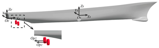
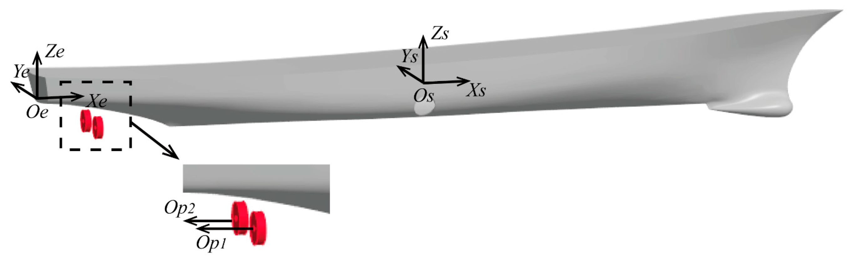
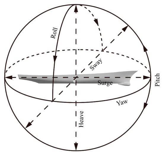
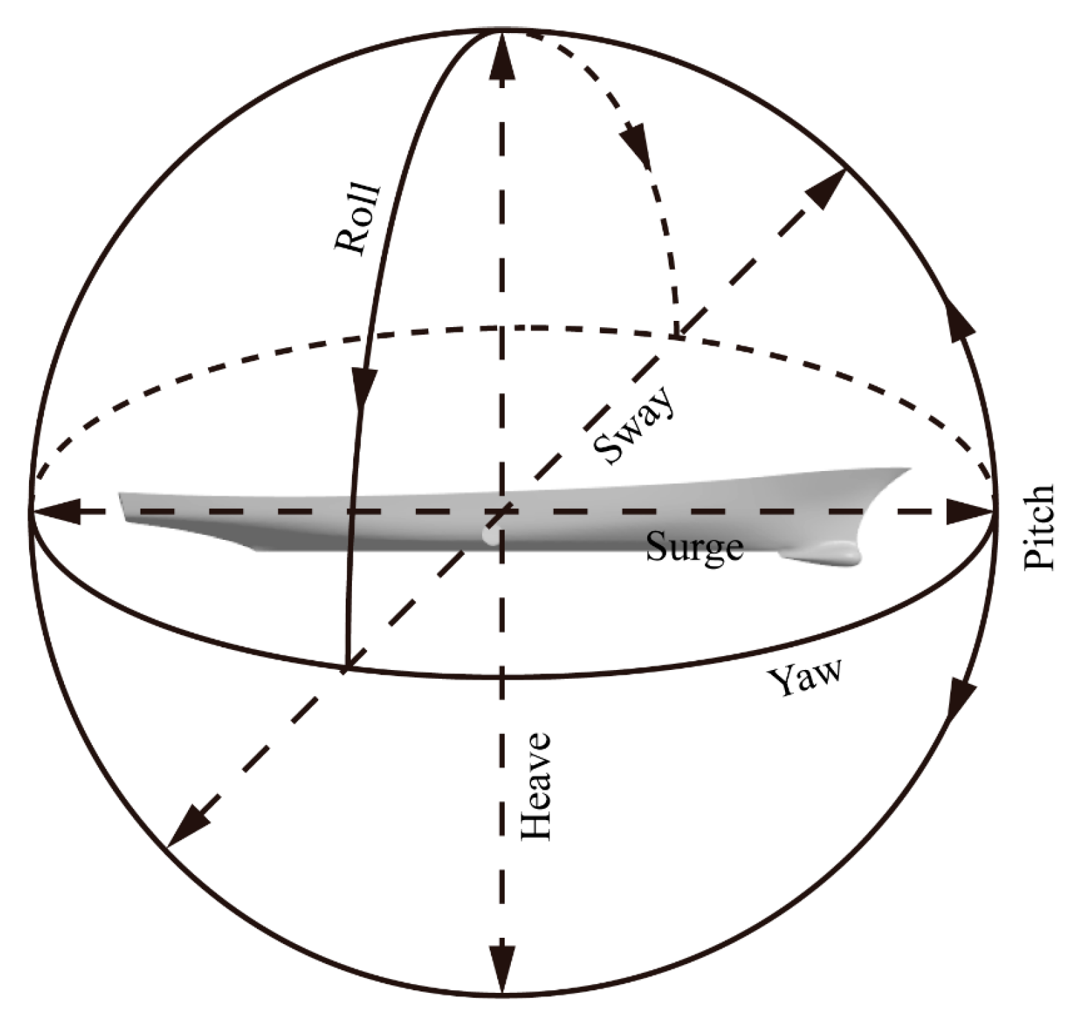
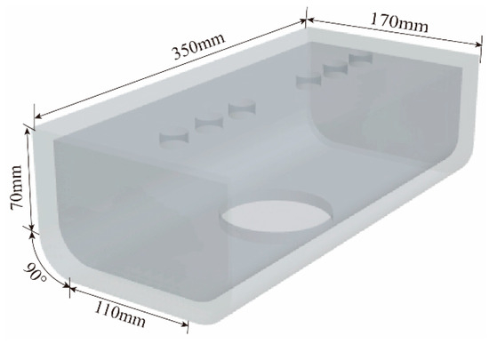
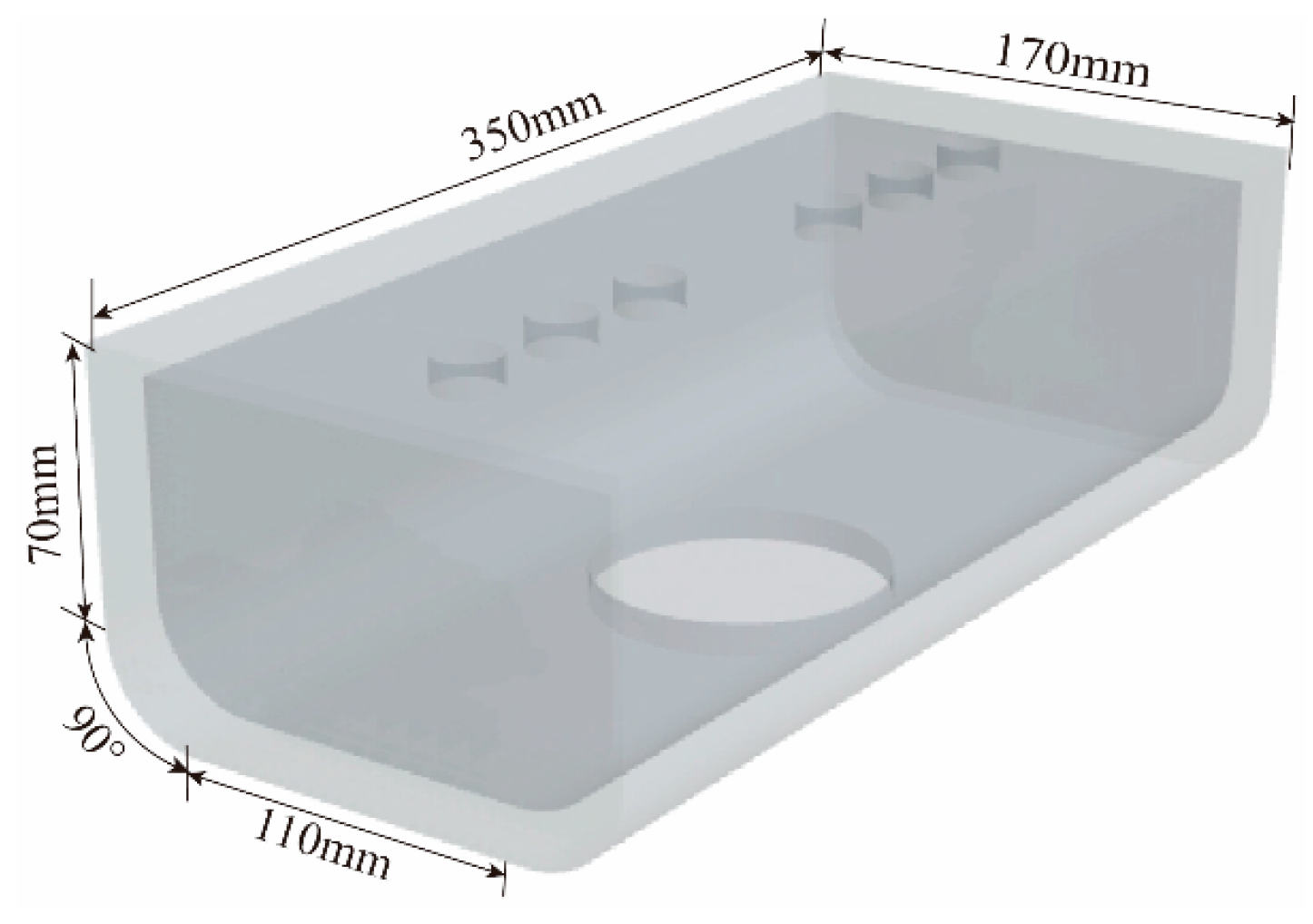
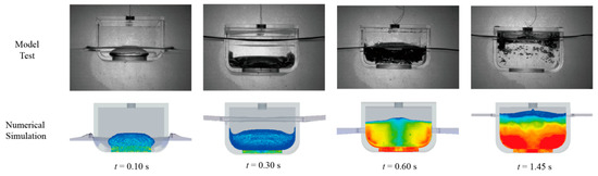
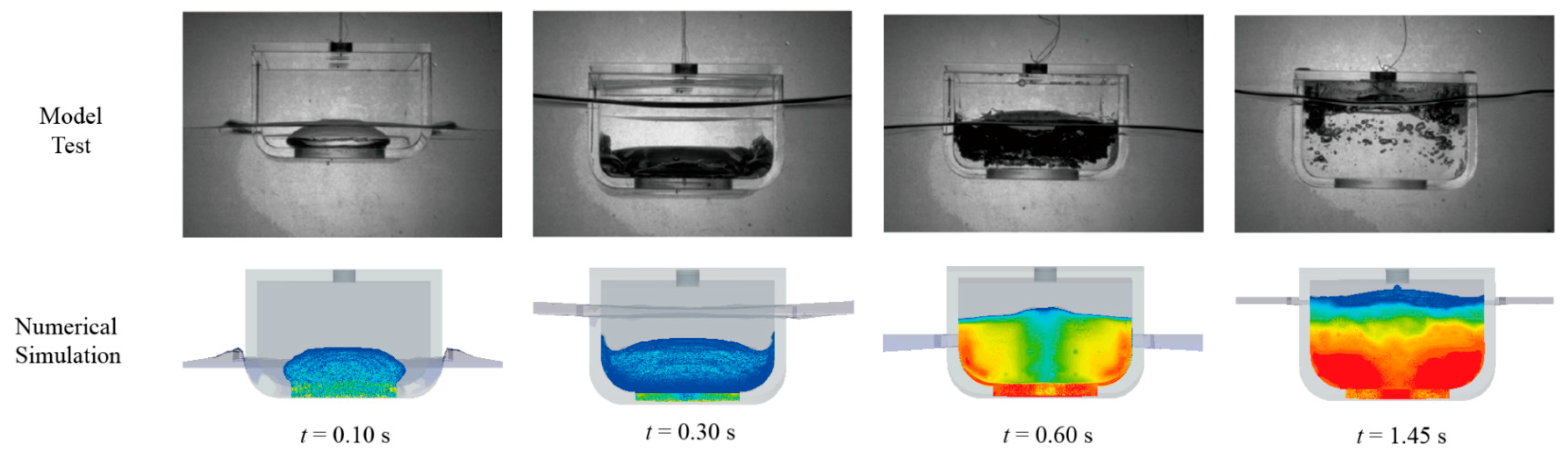
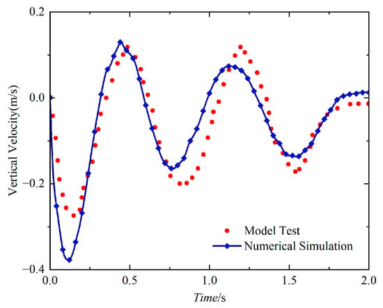
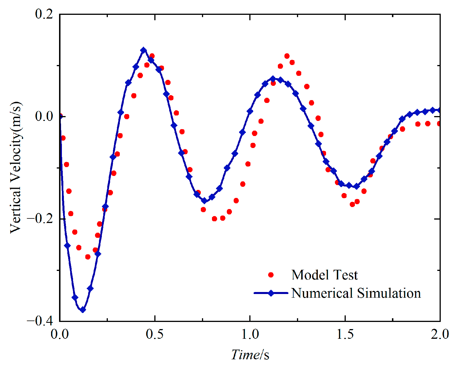
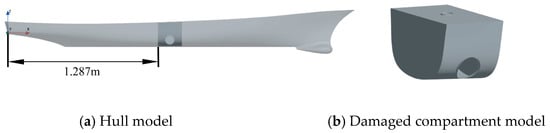
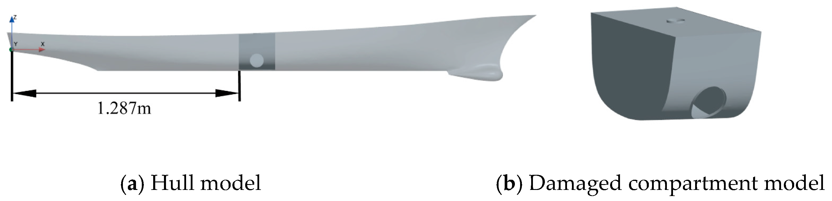


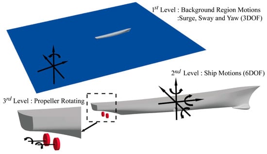
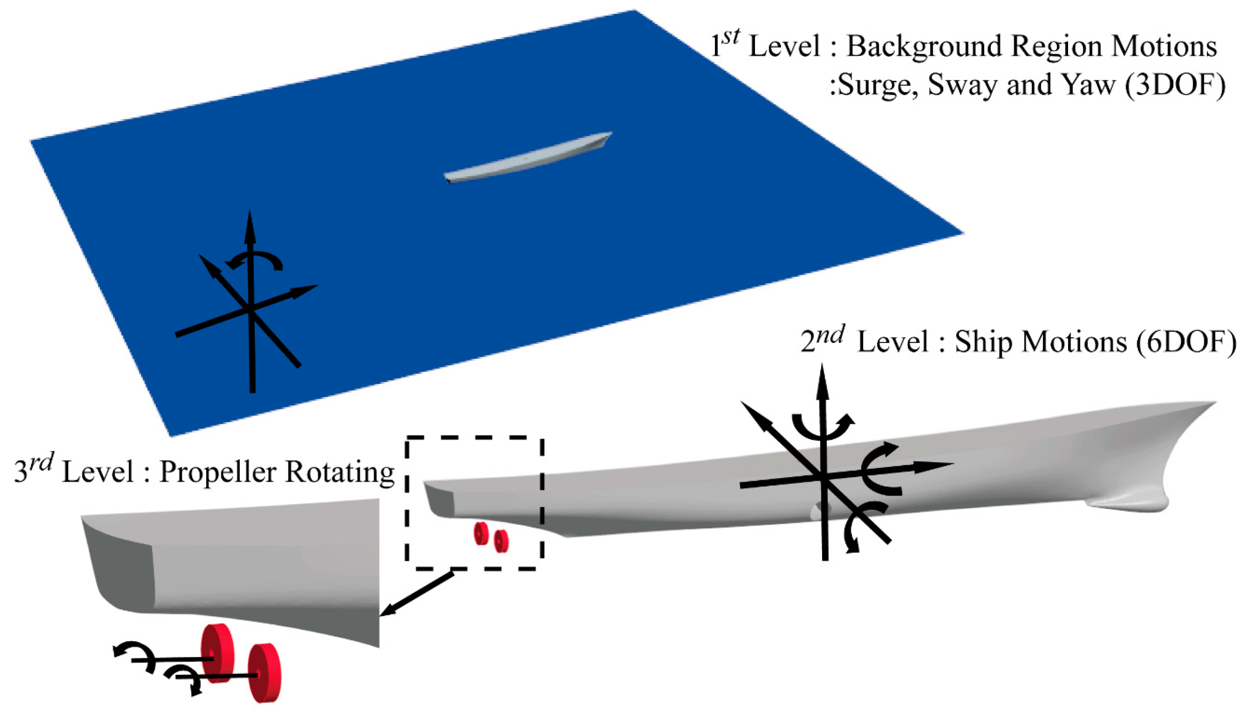
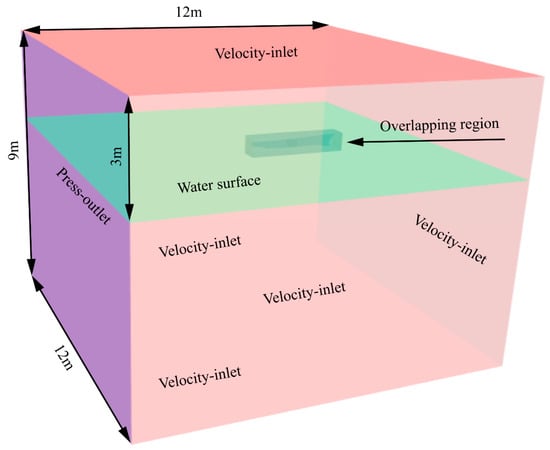
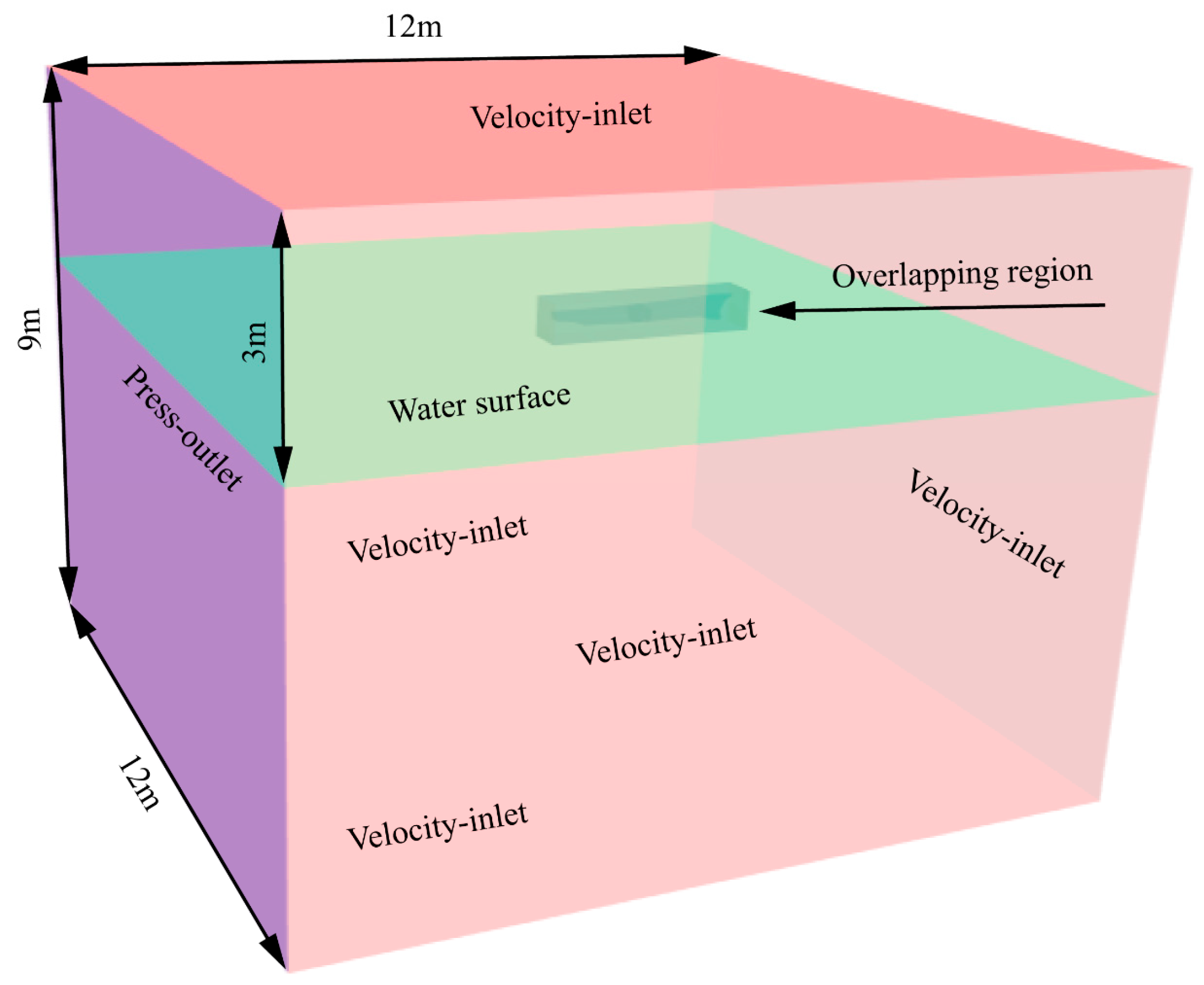
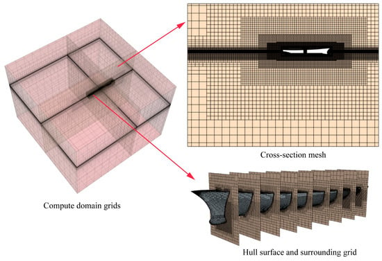
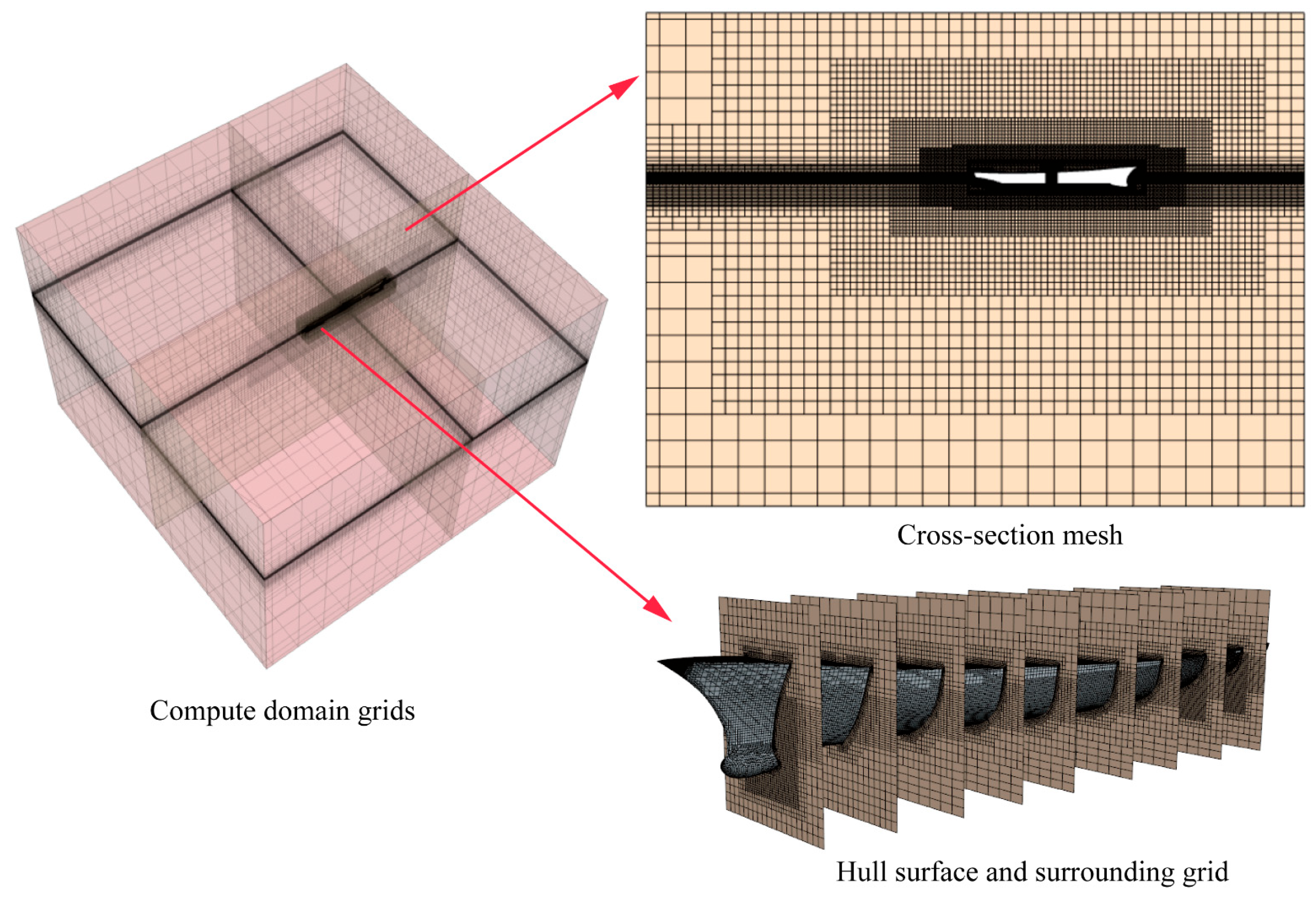
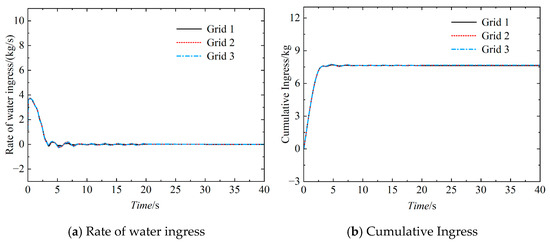
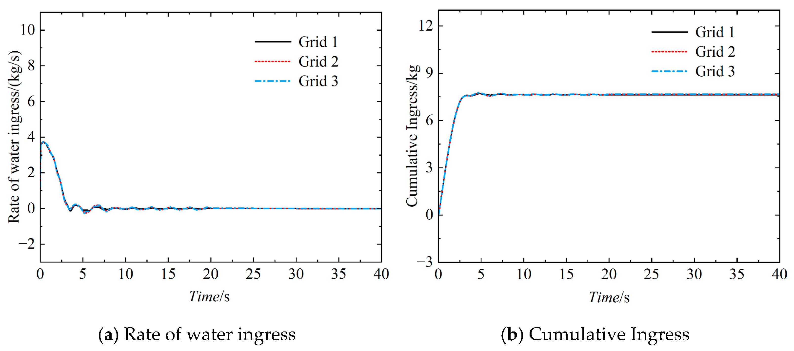
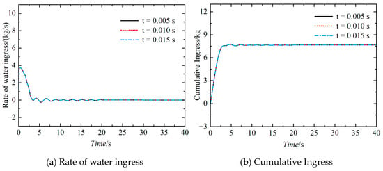
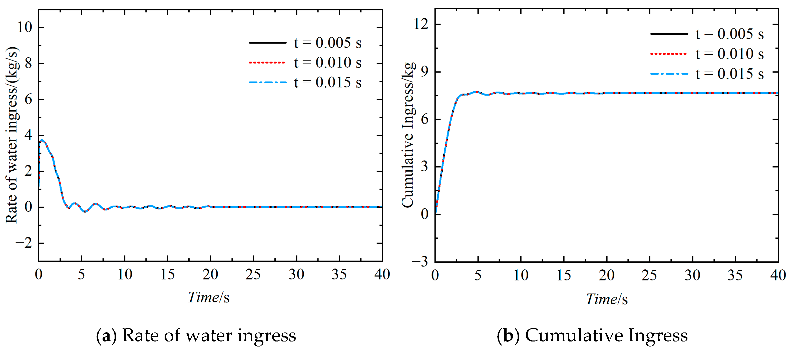
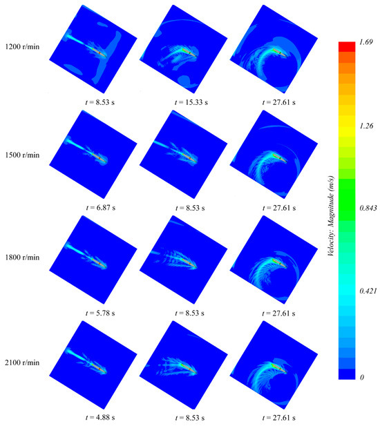
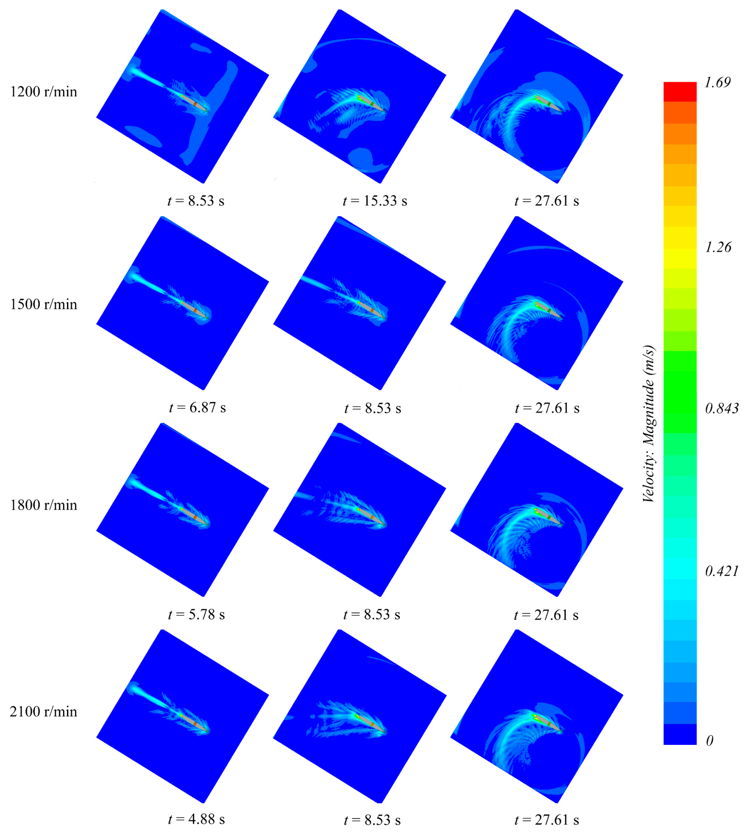
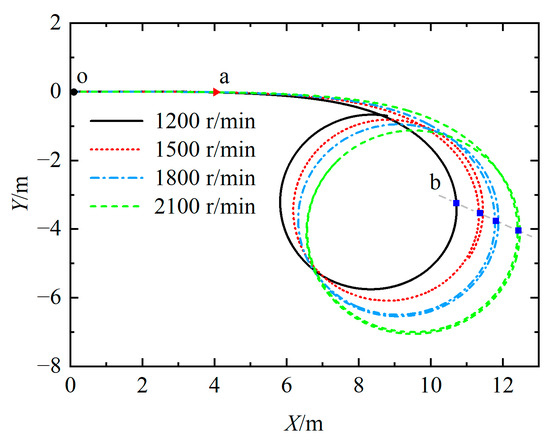
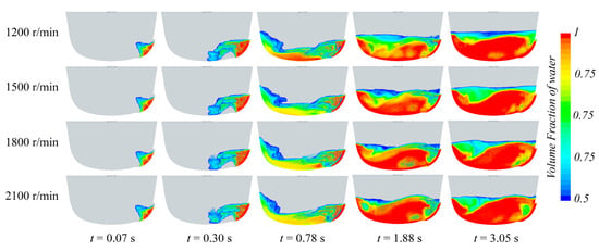
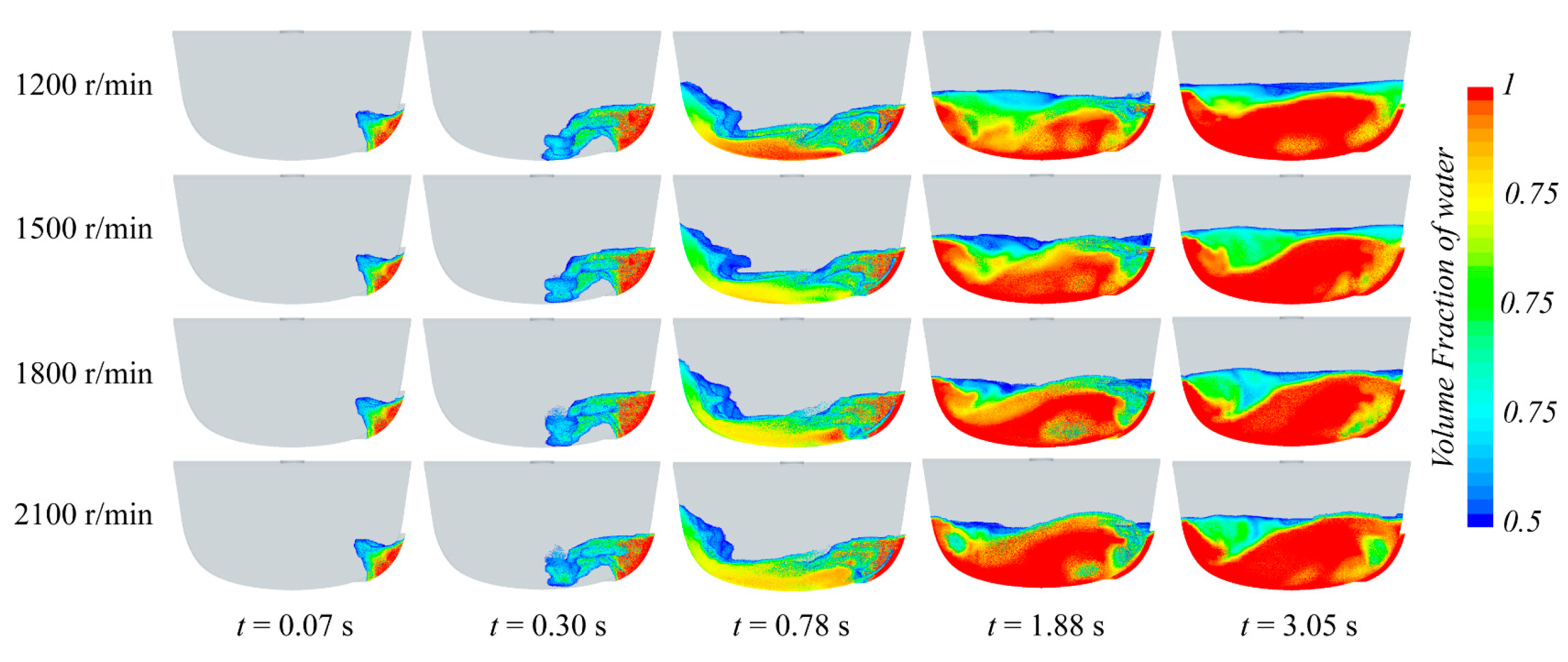
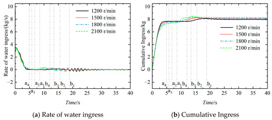
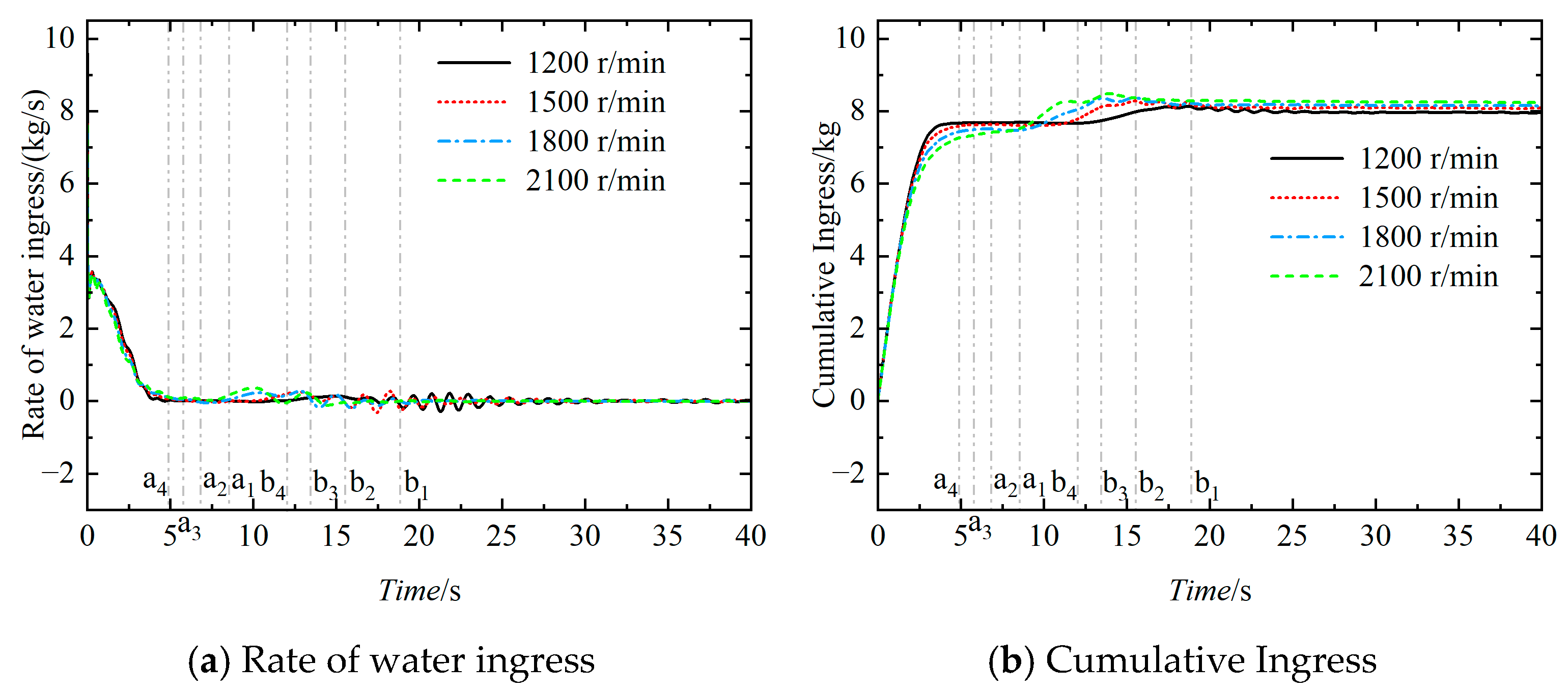
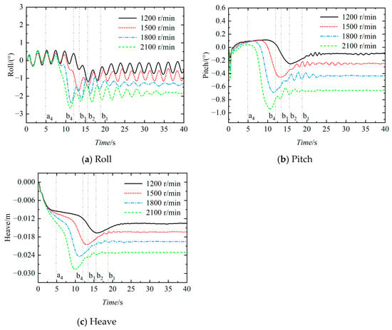
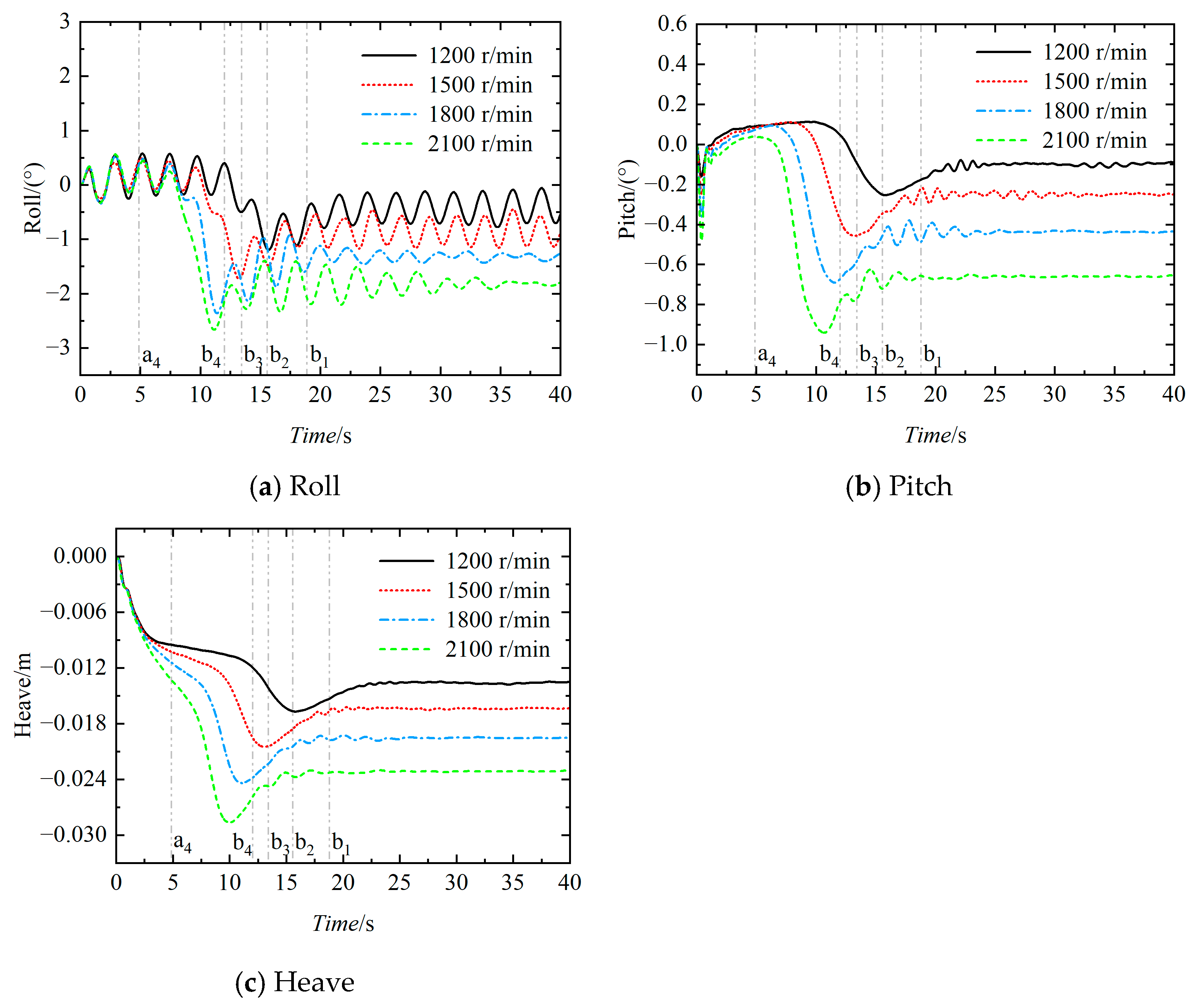
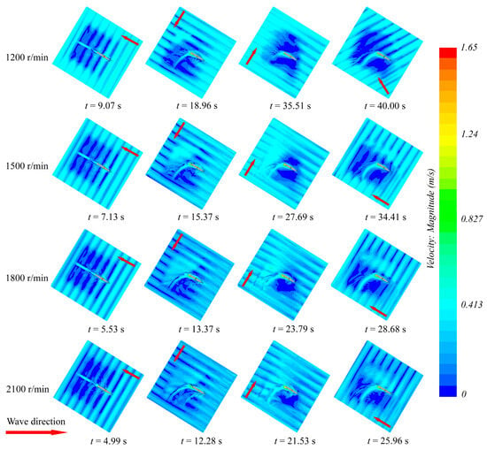
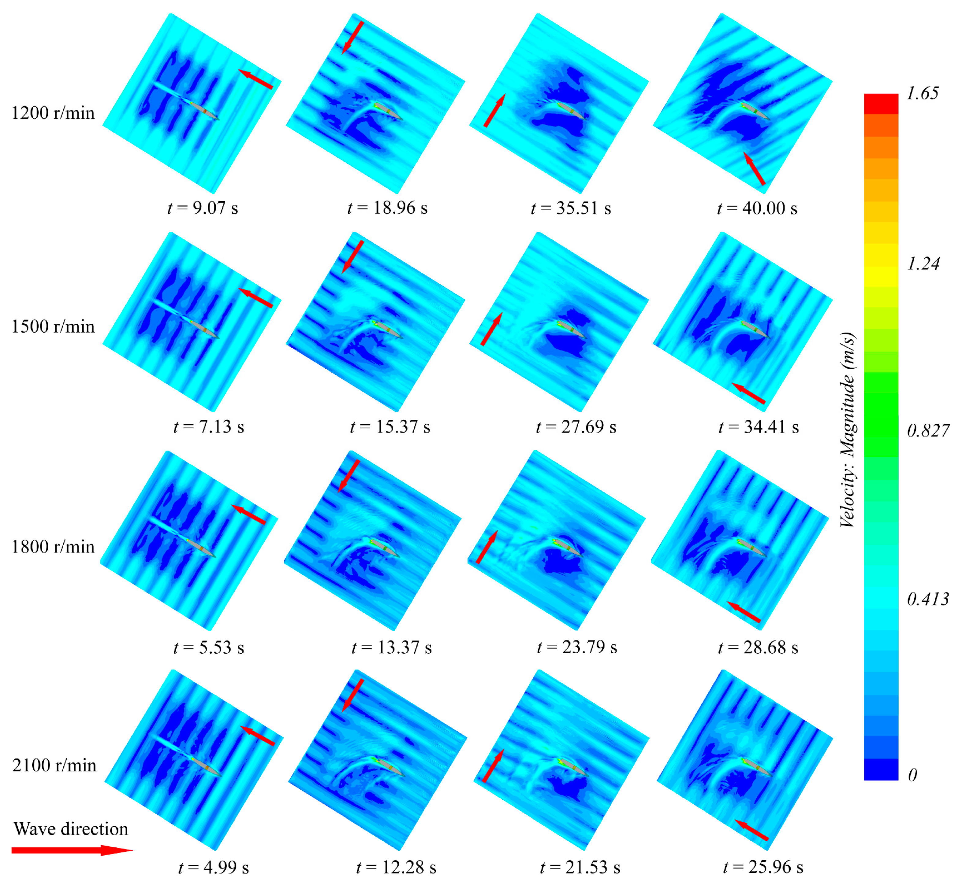
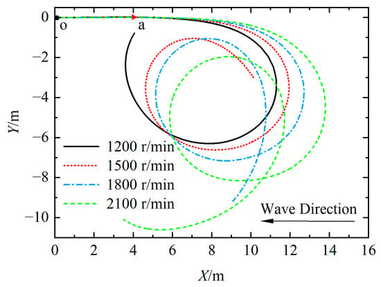
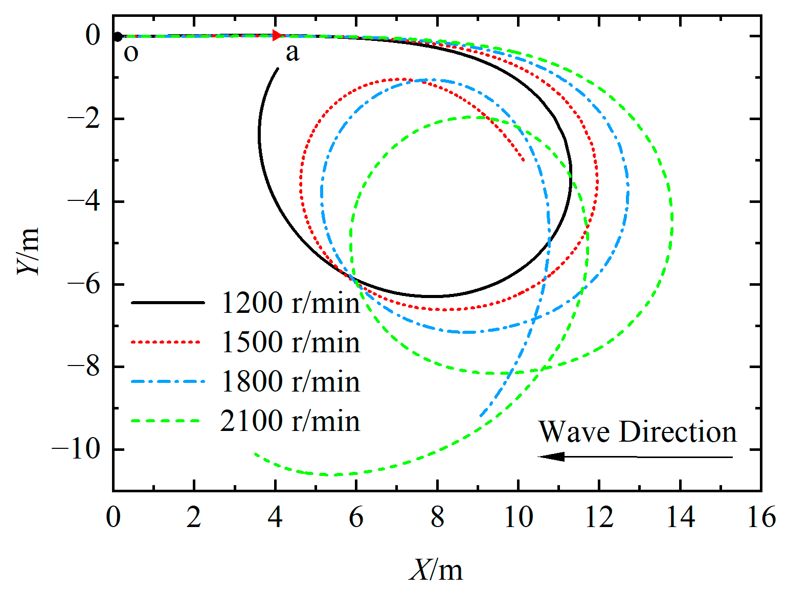
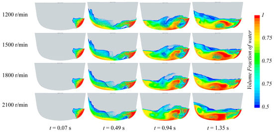
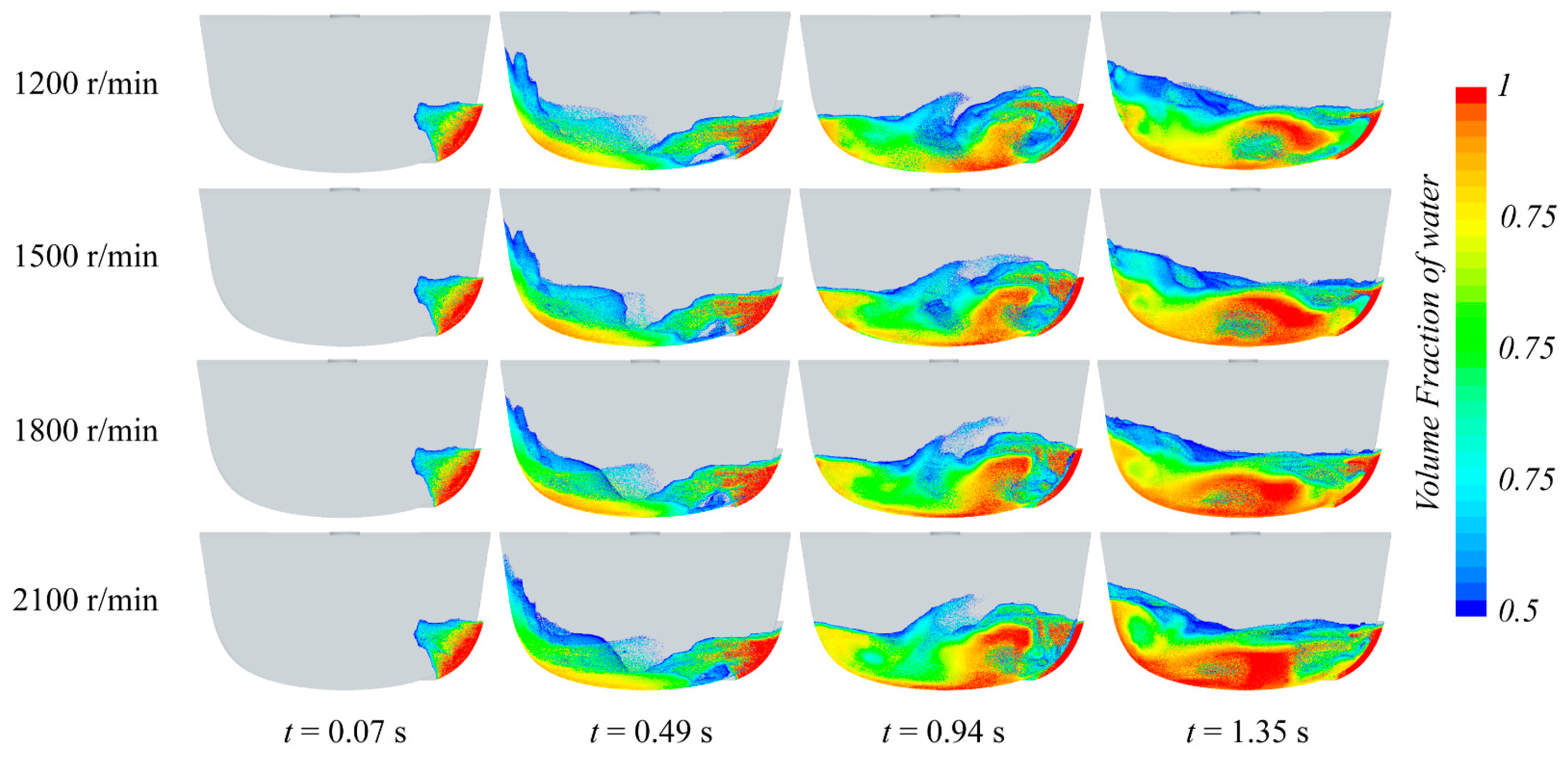
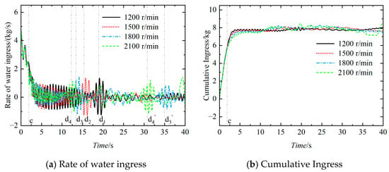
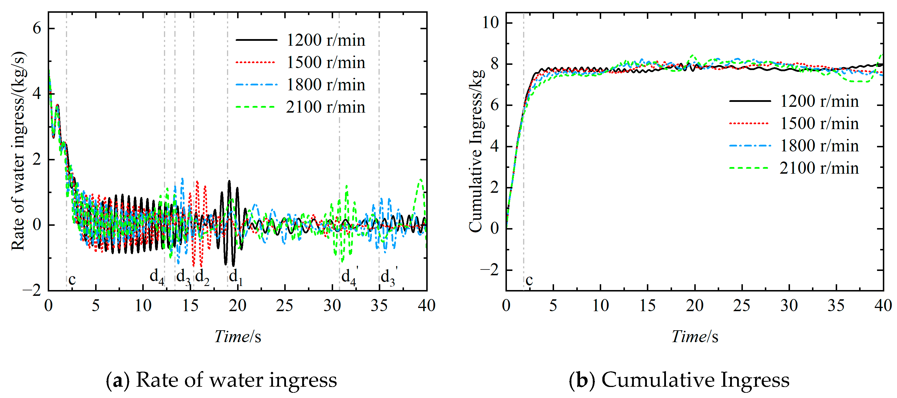
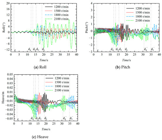
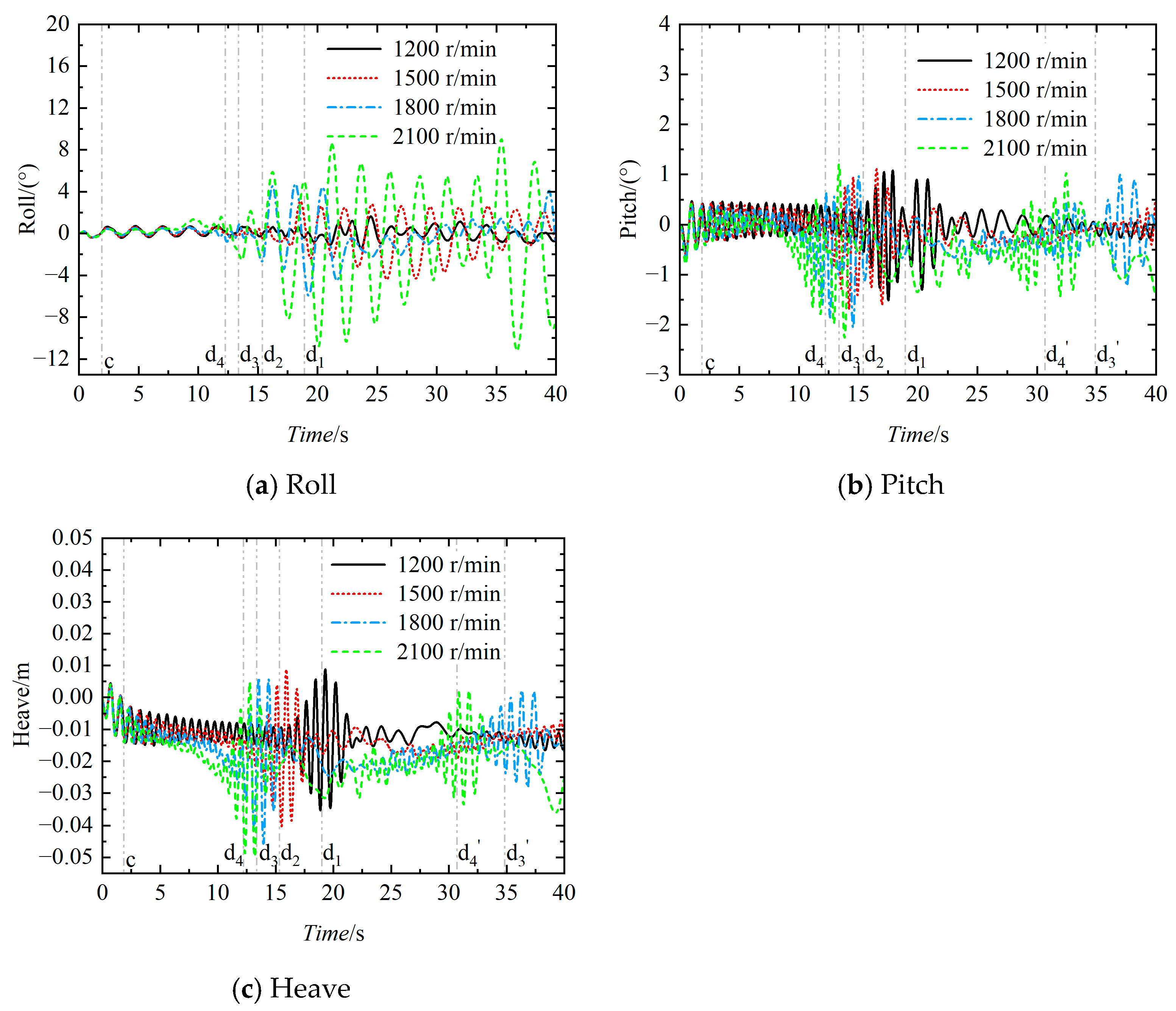
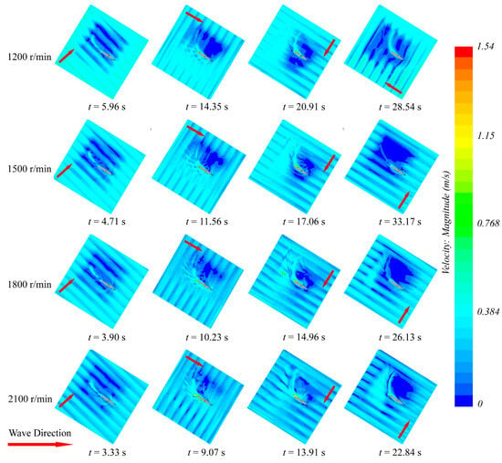
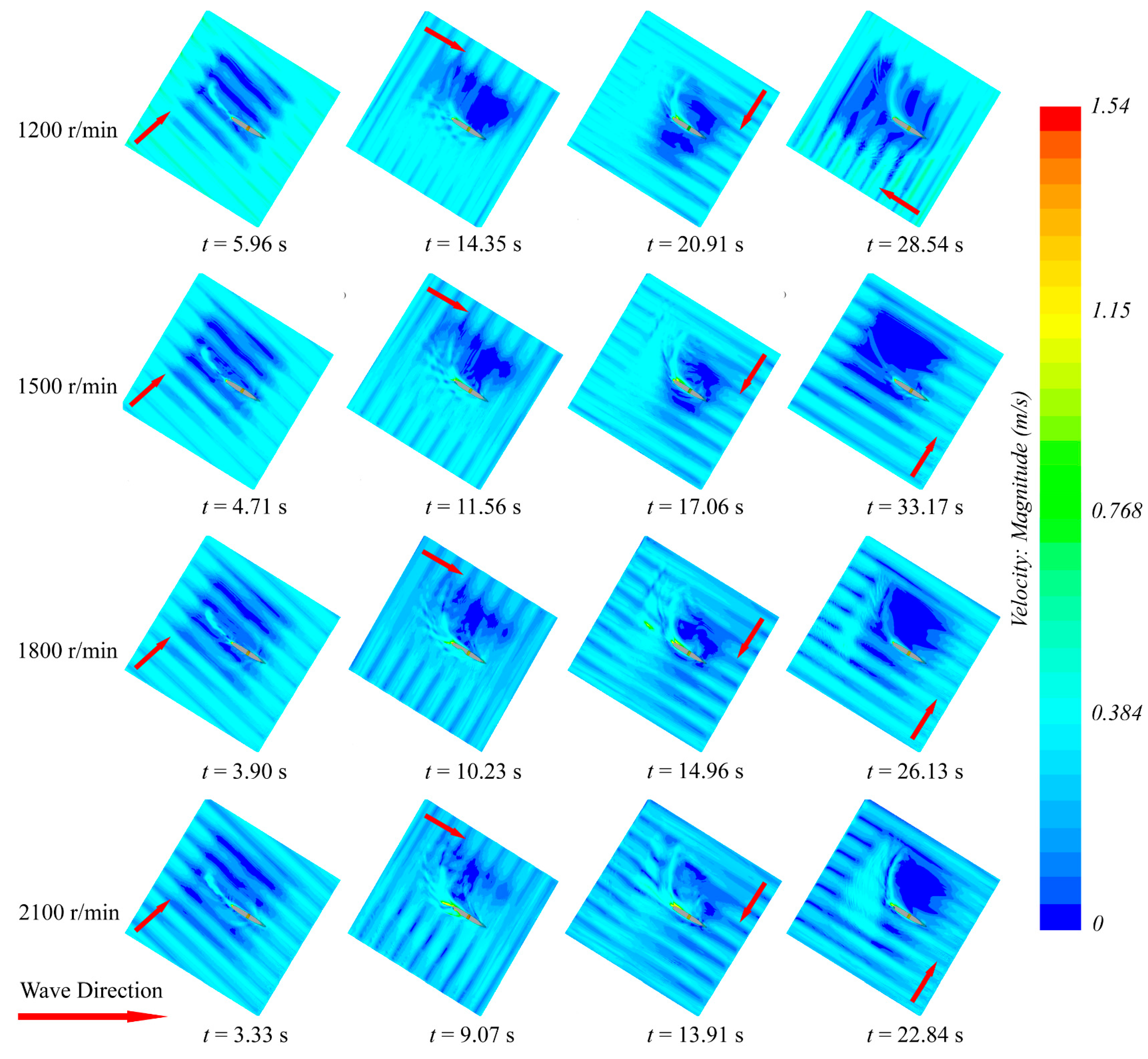
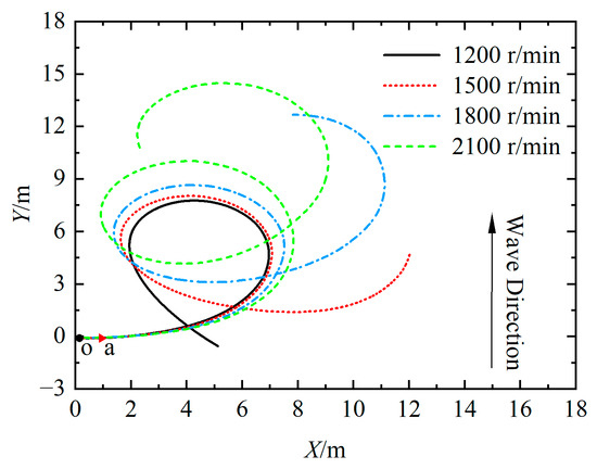
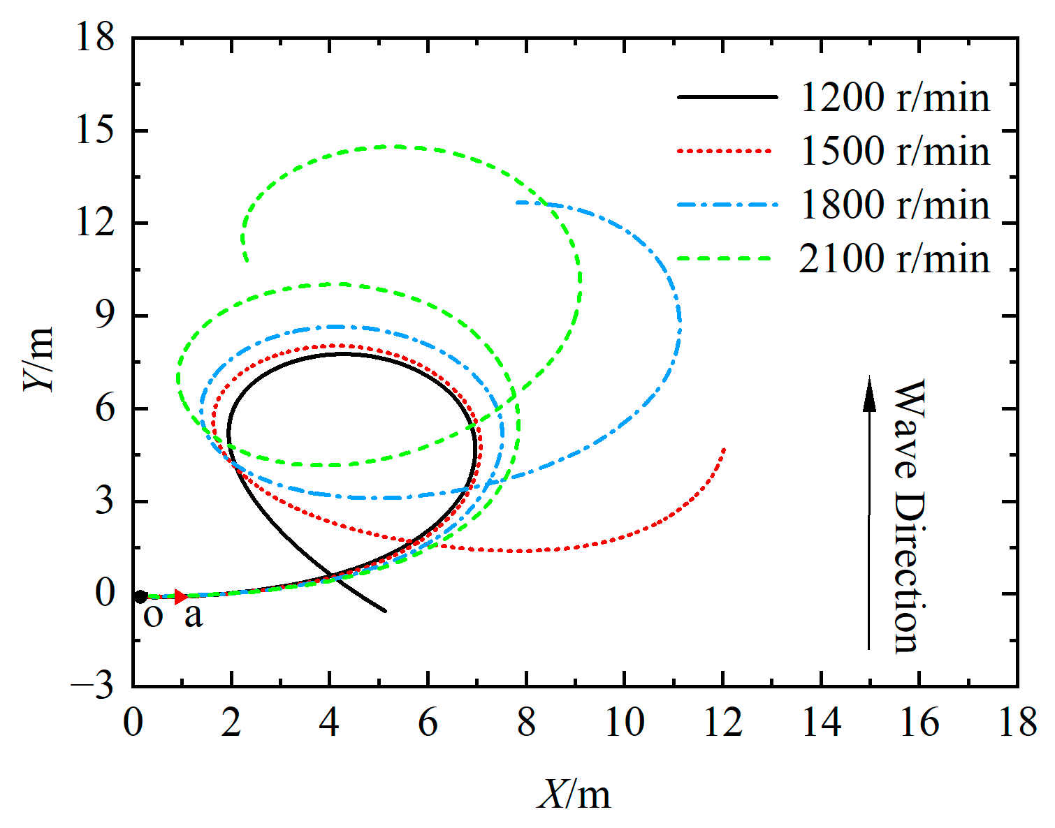
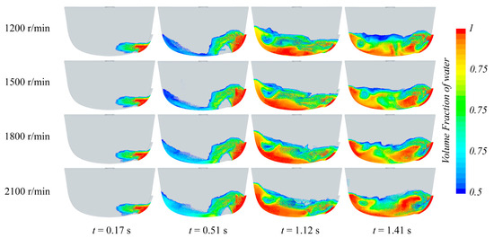
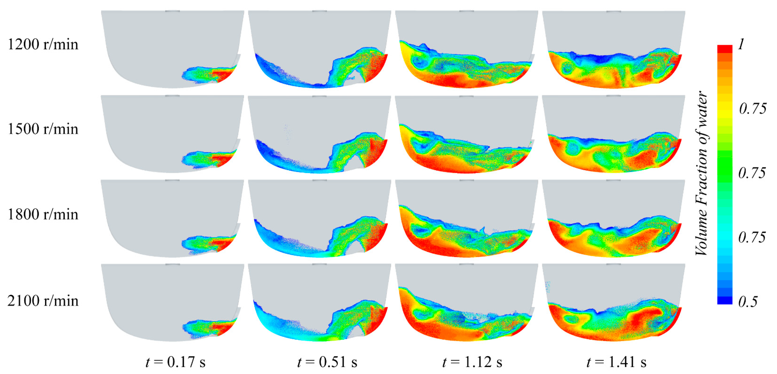
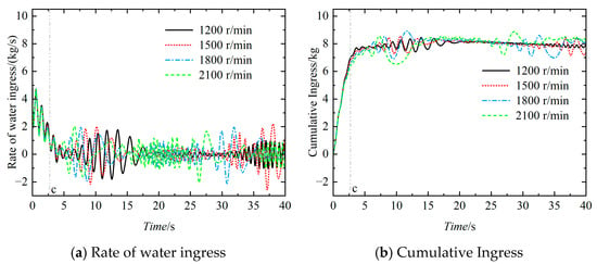
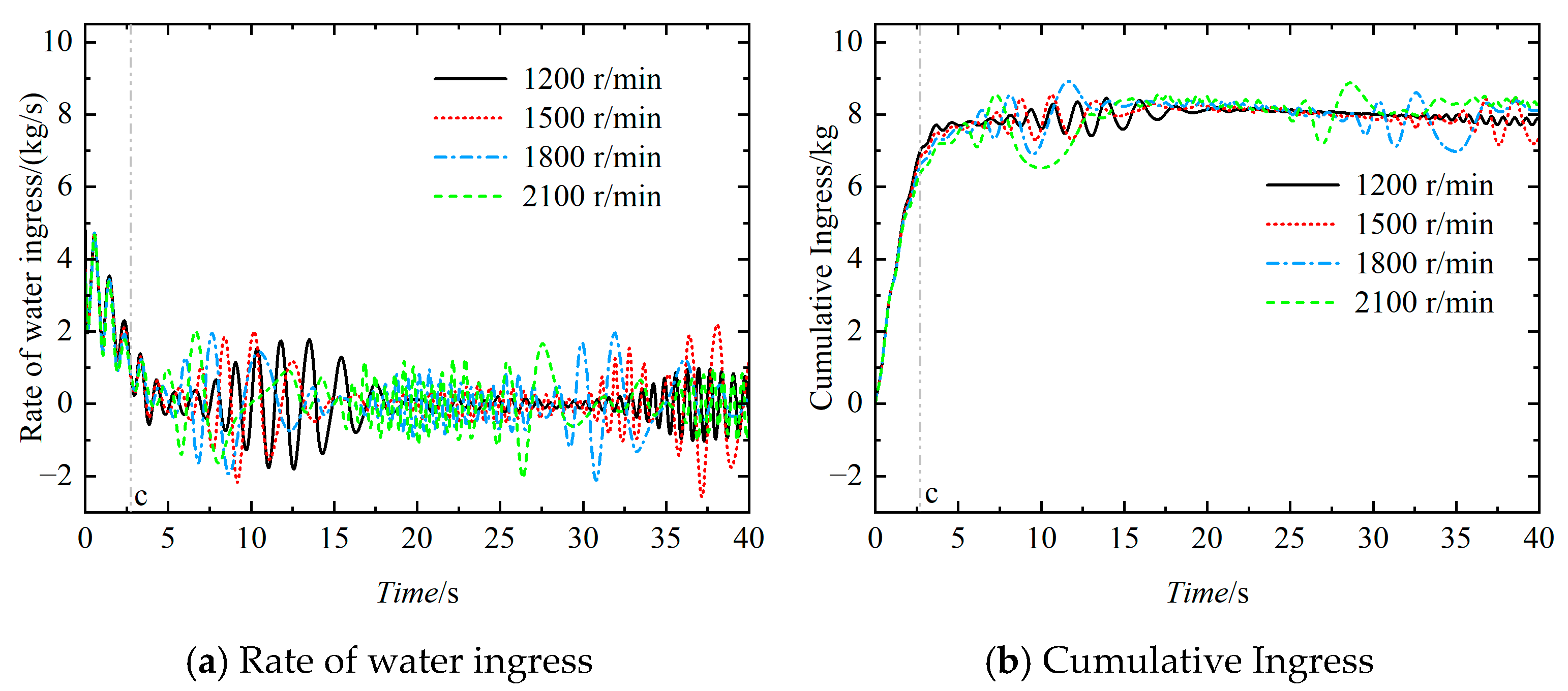
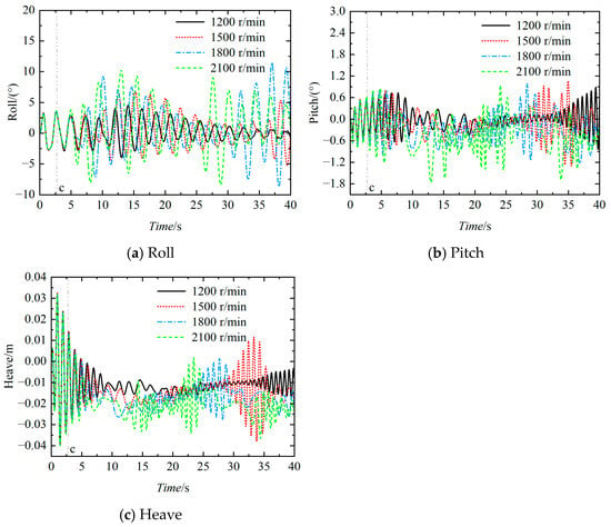
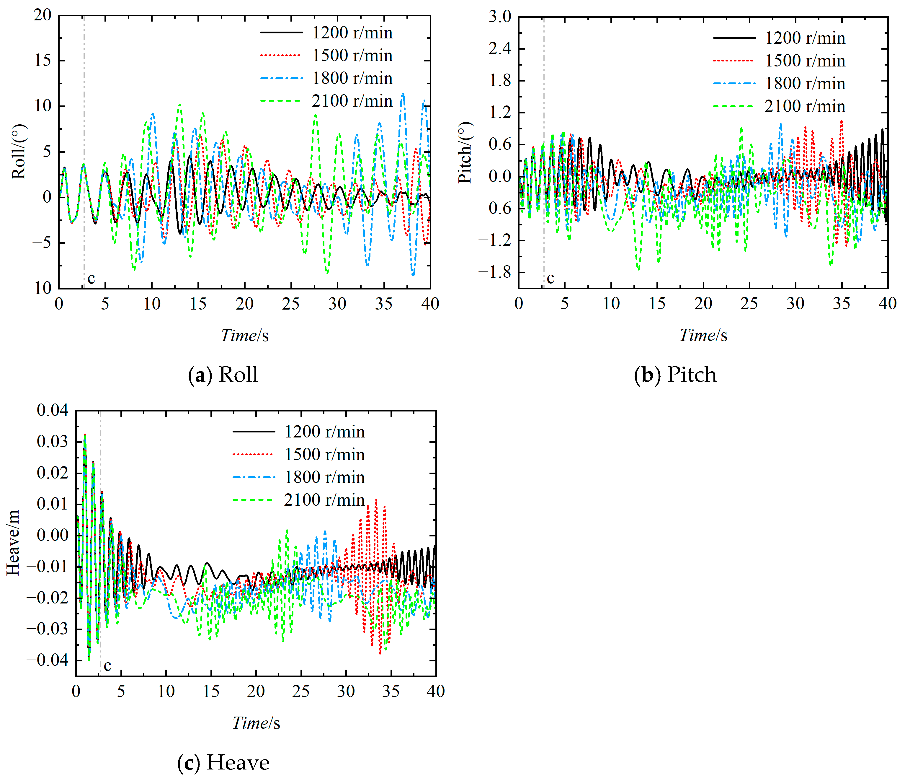

Disclaimer/Publisher’s Note: The statements, opinions and data contained in all publications are solely those of the individual author(s) and contributor(s) and not of MDPI and/or the editor(s). MDPI and/or the editor(s) disclaim responsibility for any injury to people or property resulting from any ideas, methods, instructions or products referred to in the content. |
© 2026 by the authors. Licensee MDPI, Basel, Switzerland. This article is an open access article distributed under the terms and conditions of the Creative Commons Attribution (CC BY) license.