


Abstract
For stable operation of autonomous surface ships, real-time anomaly detection of engine conditions must be coupled with an operational framework that sustains model performance in dynamic maritime environments. This study proposes an autonomous maintenance system that combines a subsystem-level condition-based maintenance (CBM) model with a dedicated MLOps framework. The main engine is decomposed into multiple functional component units, each governed by an independent diagnostic pipeline that applies a hybrid algorithm combining an attention LSTM autoencoder with an isolation forest to capture subtle anomalies. Although this hybrid attains higher precision than conventional single models, it remains sensitive to operating environment shifts. To address this, we develop an onboard MLOps pipeline that monitors distributional shifts in real-time sensor data and executes an autonomous maintenance mechanism, retraining and redeploying models on local data when performance degradation is anticipated. A dual-monitoring rule set based on a standardized deviation score and its smoothed change rate is used to discriminate abrupt mechanical anomalies from gradual drift. Experiments on a fault simulation testbed indicate that, under data drift, the system can recover detection reliability and adapt to changing engine conditions, providing a technical basis for the self-sustaining reliability of autonomous surface ships.
1. Introduction
Ships operate under exceptionally harsh environmental conditions, including continuous exposure to high temperatures, elevated pressures, severe vibrations, and corrosive seawater. Consequently, onboard mechanical systems are required to exhibit outstanding reliability and durability. Among these systems, the main engine constitutes the most critical component responsible for vessel propulsion: any malfunction or failure can lead to immediate operational downtime, posing severe threats to navigational safety and logistical continuity. Maintaining engine health through precise condition monitoring and predictive maintenance is therefore of paramount importance [1,2].
Traditionally, the maintenance of marine engines has been carried out through time-based maintenance (TBM) or planned maintenance systems (PMS) that follow fixed schedules or manufacturer guidelines [3]. However, these conventional approaches fail to reflect the real-time operational status of the machinery, often resulting in unnecessary maintenance actions or, conversely, in the omission of early failure indicators—leading to unexpected downtime and increased lifecycle costs. With the accelerating adoption of maritime autonomous surface ships (MASS) and the intensifying global shortage of seafarers, the demand for automated and intelligent condition-based maintenance (CBM) solutions has surged rapidly [4,5].
Although CBM leverages real-time sensor data to proactively detect anomalies, its application to marine main engines is challenging due to the inherent structural complexity of the system. A main engine consists of multiple dynamically interacting subsystems—including cylinders, fuel injection systems, and turbochargers—whose sensor signals are inherently multivariate and exhibit strong temporal dependencies. As a result, traditional rule-based approaches and single-model AI methods often fail to capture early-stage anomaly symptoms [6,7]. To address this, recent studies have explored deep learning-based multivariate time-series anomaly detection, including LSTM encoder–decoder architectures [7], Transformer-based association discrepancy models [8], and end-to-end deep learning frameworks tailored for marine machinery [2,9,10]. Furthermore, hybrid schemes that couple deep representation learning with isolation-based scoring have demonstrated improved robustness for malfunction detection in complex industrial systems [11,12].
A further critical challenge in deploying CBM models onboard is the issue of data drift: the statistical properties of sensor signals evolve over time due to seasonal variation, fouling, component aging, and changes in operational profile, causing offline-trained models to gradually lose diagnostic reliability [13,14]. Recent advances in MLOps have therefore emphasized the integration of drift detection, adaptive windowing, and transfer learning to sustain model performance throughout the operational lifecycle [15,16].
To overcome the masking effect of global models and improve detection resolution for subtle anomalies, this study decomposes the main engine into multi-functional subsystems guided by established physical domain knowledge of marine diesel engines [1,6]. For each subsystem, a hybrid model that combines an attention-LSTM-AE with an isolation forest is employed. This hybrid detector is embedded within an onboard MLOps framework that monitors data drift using a standardized deviation score (D) and its smoothed rate of change (). Whereas most prior modular detectors address offline detection alone and conventional streaming drift detectors typically emit only binary drift decisions, the proposed design is intended to discriminate, at the per-feature level, between abrupt mechanical anomalies and gradual degradation (e.g., natural wear and environmental shifts). By treating gradual wear as a “new normal” through autonomous model retraining, the framework seeks to reduce false alarms while logging the cumulative baseline shift such that long-term machinery degradation is not masked by successive local updates.
Building on this design, this study examines, through testbed experiments encompassing progressive degradation and abnormal operating scenarios, whether the proposed MLOps-based framework can detect subsystem-level anomalies and restore diagnostic reliability—measured by the anomaly rate ()—after data drift occurs. The main contributions are threefold: (i) a subsystem-level hybrid detector that couples attention-LSTM-AE reconstruction with Isolation Forest scoring; (ii) an interpretable, per-feature drift metric pair (D, ) that separates sudden faults from gradual drift and maps directly onto maintenance actions; and (iii) an onboard MLOps pipeline that links this metric to autonomous retraining and redeployment. Through these elements, the study aims to provide a technical basis for the self-sustaining reliability required by autonomous surface vessels.
2. Related Work
This study aims to develop an intelligent condition monitoring and MLOps framework for the main engines of Maritime Autonomous Surface Ships (MASS). To this end, this section reviews existing literature on ship engine anomaly detection techniques, deep learning-based hybrid models, and the application of MLOps and data drift management in industrial systems. In doing so, this section distinguishes four related but distinct strands of research: predictive maintenance as the overarching application goal, anomaly detection as the technique for identifying deviations from normal behavior, drift adaptation for responding to non-stationary data distributions, and continual learning for updating models without catastrophic forgetting. The proposed framework is positioned as an anomaly detection model coupled with a drift-adaptive, self-retraining MLOps pipeline, rather than as a full continual-learning method.
2.1. Ship Engine Anomaly Detection and Condition-Based Maintenance (CBM)
Traditional ship engine maintenance has relied largely on time-based maintenance (TBM); however, advances in sensor technology and Internet of Things (IoT) have supported a shift toward condition-based maintenance (CBM), which has become increasingly relevant for unmanned environments such as MASS [1,4]. Early CBM research primarily used thresholds based on expert domain knowledge or rule-based algorithms [3]. Given the interdependencies among numerous cylinders, turbochargers, and fuel injection systems within a ship’s main engine, however, single-sensor thresholds alone may be insufficient to capture non-linear failure mechanisms [6].
Accordingly, deep learning has been applied to multivariate time-series analysis for anomaly detection in marine machinery [2,9]. Recurrent neural networks (RNN) and long short-term memory (LSTM) models were widely used in earlier work [7], but they can suffer from vanishing long-term dependencies in lengthy time series and from difficulty in mapping complex correlations among multivariate sensors. To address these issues, more recent studies have adopted Transformer architectures and attention mechanisms, which extract spatio-temporal features from multivariate machinery data in parallel and have reported improved early detection of subtle faults [8,10]. More recently, adversarial autoencoder schemes such as Bi-AAE [17] and graph-based architectures that model inter-sensor topology [18] have also been proposed for marine diesel engines, with the aim of detecting fault patterns that propagate across coupled subsystems.
Beyond marine engines, related work on rotating machinery has explored knowledge-enhanced and uncertainty-aware degradation models; for instance, a signal knowledge-enhanced domain adaptation network has been proposed for remaining useful life prediction and uncertainty quantification of rolling bearings [19], illustrating the broader trend toward physically informed, transferable diagnostic models for mechanical systems.
2.2. Hybrid Models and Subsystem-Level Diagnosis
Hybrid architectures that combine deep learning with ensemble methods have been reported to perform well in complex industrial anomaly detection. Attention-augmented autoencoders can capture both spatial correlations and long-term temporal dependencies in multivariate sensor data, while isolation forest offers statistical evaluation of reconstruction errors in high-dimensional spaces [11,12]. Several studies have examined the complementarity of autoencoder–isolation forest pipelines, in which the AE component compresses the normal operating manifold and the IF component performs density-aware scoring on the residual space, reporting lower false alarm rates than either component used alone [20]. In parallel, hybrid LSTM-autoencoder and transformer-encoder pipelines have been used for asset-level predictive maintenance in manufacturing, where combining recurrent reconstruction with attention-based context modeling has been associated with improved robustness to noisy industrial signals [21].
Applying a single global model to an entire engine can also give rise to a “masking effect,” in which localized incipient faults are overwhelmed by normal variance. To mitigate this, several studies have adopted subsystem-level (modular) approaches. In line with this direction, the present study decomposes the main engine into multiple functional units. Whereas many prior modular approaches focus on offline detection, the present framework additionally couples the subsystem-level attention-LSTM-AE + isolation forest model with a real-time MLOps pipeline for drift detection and model retraining, as detailed in Section 4.2 and Section 5.2.
2.3. Data Drift and MLOps Application
AI models that perform well in controlled laboratory settings are often affected by data drift, in which the statistical distribution of the data changes gradually due to mechanical aging, sensor degradation, and seasonal environmental shifts [13,14]. In dynamic environments such as maritime vessels, such drift can increase the False Positive Rate of AI models and thereby reduce system reliability. In the broader context of degradation modeling, state-space formulations with adaptive drift coefficients have also been studied for tracking such gradual changes; for example, a dual adaptive drift coefficient state space model with autocorrelation-based prediction error correction has been applied to performance degradation assessment of mechanical systems [22], capturing time-varying degradation trends in a manner complementary to data-driven drift detection. To sustain long-term reliability under non-stationarity, recent surveys discuss continual learning strategies (regularization-based, replay-based, and architectural) for predictive maintenance pipelines [23], and position drift-aware retraining as a core capability of industrial MLOps [16].
A range of online drift detection methods has been proposed. Classical approaches such as ADWIN [15], the Page–Hinkley test and the cumulative sum (CUSUM) control chart [24], the drift detection method (DDM) [25], and Hoeffding’s drift detection method (HDDM) [26] are designed for streaming data and can detect concept drift in real time by monitoring statistical changes in univariate or multivariate streams [27]. Distribution-comparison methods, including the windowed Kolmogorov–Smirnov (KS) test [28], maximum mean discrepancy (MMD) [29], and the population stability index (PSI) [30], are also applied in a sliding-window manner for batch-wise detection. These methods generally output binary drift decisions (drift or no drift), and they typically do not distinguish between mechanical faults that require immediate physical inspection and gradual environmental drift that calls for model retraining. In addition, many of them provide limited per-feature interpretability, which can make it difficult for marine engineers to identify which sensor or subsystem is primarily responsible for a detected shift.
Building on these methods, the present framework operates in a real-time batch-wise manner (batch size of 100 with 80-step overlap) and uses a per-feature standardized deviation score () together with its EWMA-smoothed rate of change (). The intent is to detect distributional shifts online, in a manner comparable to ADWIN and windowed KS-test/MMD, while additionally supporting interpretable, rule-based discrimination between “Sudden Anomalies” and “Gradual Drift” through thresholds aligned with conventions familiar to marine engineers. The framework simultaneously monitors the anomaly rate () derived from the isolation forest, providing a unified decision logic for autonomous onboard MLOps. While the autonomous retraining pipeline proposed in this work shares the goal of sustaining model validity under non-stationarity, it is distinct from continual learning in the strict sense: rather than employing regularization- or replay-based mechanisms to prevent catastrophic forgetting across a continuous stream of tasks, the framework treats drift as a discrete trigger that initiates a controlled retraining cycle on a curated data buffer. It therefore occupies the boundary between drift adaptation and continual learning, emphasizing interpretable, rule-based triggering suitable for safety-critical onboard operation. A quantitative comparison with the streaming drift detectors discussed above, under identical batch-wise conditions, is presented in Section 6.6.
3. Subsystem-Level Anomaly Detection Model
The framework proposed in this study introduces a modular subsystem-level detection architecture that integrates physical domain knowledge-based data structuring. This approach moves beyond the conventional single global model methodology to enable precise anomaly detection in complex environments such as ship main engines [12].
3.1. Data Acquisition and Feature Extraction
3.1.1. Testbed and Sensor Configuration
To develop and validate the anomaly detection framework, sensor data were acquired using a failure simulation testbed consisting of a MAN B&W 6S46MC-C7 two-stroke low-speed engine and a Fuchino CFSR 20.0 dynamometer capable of controlling loads up to 7400 kW.
Data were collected through three independent sensor systems: an alarm monitoring system (AMS) capturing analog and digital operating signals in real time, a Performance measurement indicator (PMI) measuring in-cylinder combustion pressure at a high sampling rate, and a vibration monitoring system (VMS) recording structural vibrations of the engine. The signals were acquired through a National Instruments CompactDAQ chassis (cDAQ-9189) with dedicated analog input modules; the overall instrumentation and signal flow are illustrated in Figure 1, and the channel configuration for the No. 1 cylinder system is summarized in Table 1. The cylinder-pressure (PMI) channels were sampled at 33.3 kS/s/ch (NI 9253, 24-bit), while temperature, vibration, and crank angle signals were acquired through the remaining modules and the engine-installed monitoring systems. All raw signals were subsequently aggregated and downsampled to 1 Hz to ensure consistent multi-modal alignment for downstream analysis.
Figure 1.
Instrumentation and data acquisition architecture of the engine condition-monitoring system.
Table 1.
Data acquisition configuration for the No. 1 cylinder system (two-stroke engine).
The combined instrument-level uncertainty of the acquisition chain is on the order of a few percent of the measured value (e.g., 0–350 bar cylinder-pressure sensors at 61.68–63.03 A/bar, and accelerometers at 100 mV/g ). Because the diagnosis logic operates on standardized deviations (D) from a per-channel baseline rather than on absolute readings, this uncertainty is largely absorbed by the baseline normalization. It nonetheless sets a lower bound on the smallest detectable condition change and was taken into account when configuring the warning threshold.
3.1.2. Domain-Specific Feature Extraction
To characterize the engine’s operating state, a total of 308 features were extracted across the three domains. In this study, however, 22 core features directly related to the “No. 1 Cylinder System” were used to validate the proposed framework and to limit dilution of localized fault symptoms. The detailed items are summarized in Table 2.
Table 2.
Summary of extracted features by system category.
Direct processing of this high-frequency raw data imposes a significant computational burden and limits real-time deployment in maritime communication networks with limited bandwidth. Therefore, a feature-based preprocessing technique was applied to downsample the high-frequency PMI and VMS data to 1 Hz, matching the AMS data resolution. Specifically, cycle-level features (e.g., , ) are computed on the raw 30 kHz pressure traces on a per-cycle basis, and the most recent cycle within each 1 s window is retained as the 1 Hz representative value. Vibration-domain features (, , , etc.) are computed over each 1 s window of the raw 16–32 kHz signal. This procedure preserves intra-cycle dynamics at the feature level despite the 1 Hz aggregation rate.
For AMS data, key parameters representing the thermal and fluid dynamic state of the component were selected from the 152 signals captured in real time (Table 3). From PMI data, six physics-informed features were extracted, including maximum combustion pressure, pressure curve area, and crank angle difference (Table 4). From VMS data, six core indicators were derived in both the time and frequency domains, namely maximum amplitude, RMS, and frequency center (Table 5). Finally, to suppress sensor noise and reflect temporal dependencies, the data underwent standard scaling and were segmented using a 60 s sliding-window technique before being used as input to the diagnostic model.
Table 3.
Feature parameters of cylinder temperature data (AMS).
Table 4.
Feature parameters of cylinder pressure data (PMI).
Table 5.
Feature parameters of vibration data (VMS).
3.1.3. Low-Load Filtering
In low-load and idle operating regimes (typically below 25% of rated load, corresponding to engine speeds under 30 RPM in the testbed), sensor signals tend to be unstable due to incomplete combustion and irregular fuel injection, resulting in noisy measurements that do not reflect the engine’s normal operating behavior. If such unstable data were included in the baseline reference statistics (, ), the resulting reference distribution could be distorted and could cause false anomaly alarms during online inference. To limit this effect, a filtering rule was applied that excludes all samples acquired under engine speeds below 30 RPM, and the same rule is enforced consistently during both the initial baseline training phase and the online inference phase, so that the model evaluates only the steady-state operating regime in which the sensor signals and the physics-based derived features remain reliable.
3.1.4. Drift-Aware Derived Features
To capture the dynamic behavior of the engine in a maritime environment and to improve robustness against environmental drift, three physics-informed derived features were constructed from the raw sensor parameters.
- Combustion Efficiency Indicator (Feature_Pmax_Efficiency): the maximum in-cylinder pressure () is normalized by the current engine speed (RPM) to track combustion performance, i.e., .
- Thermal Load Sensitivity (Feature_Temp_Sensitivity): the ratios of exhaust gas temperature and cylinder liner temperature to engine speed (RPM) are computed to detect changes in the heat-exchange efficiency of the cooling system, i.e., .
- Vibration Sensitivity per Load (Feature_Vib_per_Load): the ratio of vibration energy (RMS) to the fuel index is monitored to track incremental mechanical friction or wear, i.e., .
To examine the statistical and physical characteristics of the proposed derived features, a sensor correlation heatmap was generated, as shown in Figure 2. The traditional primary variables exhibit strong positive correlations with one another (red regions), reflecting multicollinearity driven by the common dependence on engine speed and load. In contrast, the three proposed derived features (highlighted in red boxes) display different correlation profiles: Feature_Pmax_Efficiency and Feature_Vib_per_Load show negative correlations with the RPM and fuel index columns, indicating that the load-normalization reduces the dominant operational dependency, while Feature_Temp_Sensitivity exhibits near-independent behavior across most raw variables. These correlation structures suggest that the derived features carry diagnostic information that is not redundantly encoded in the raw sensors, thereby complementing the existing feature space.
Figure 2.
Correlation heatmap demonstrating the characteristics of the proposed engineered features. The red boxes highlight the three proposed derived features (Feature_Pmax_Efficiency, Feature_Temp_Sensitivity, and Feature_Vib_per_Load).
3.2. Decomposition into Functional Component Units
The conventional approach of feeding hundreds of multivariate sensor signals into a single global neural network for anomaly detection has structural limitations. In particular, it gives rise to a so-called “masking effect,” in which subtle incipient faults originating from specific components are obscured by the normal variance of the system as a whole, thereby degrading the detection sensitivity of the model.
To address this, the proposed framework adopts a subsystem-level architecture that decomposes the engine into functional component units based on physical domain knowledge, and assigns a dedicated deep learning model to each unit (Figure 3). In the present testbed, the main engine is divided into 14 functional units, whose per-domain feature counts are summarized in Table 6. Each unit is monitored by an independent detector trained with the same attention-LSTM-AE + isolation forest pipeline, so that a localized fault is assessed against the reference behavior of its own subsystem rather than being diluted within a single global model.
Figure 3.
Proposed subsystem-level architecture of the main engine.
Table 6.
Decomposition of the marine main engine into 14 functional component units and the number of features per sensor domain.
This study validates the framework using the No. 1 Cylinder System as a representative case. This choice is motivated by the structural homogeneity of the six cylinder units: as shown in Table 6, the No. 1 through No. 6 cylinder systems share an identical sensor and feature configuration (12 AMS, 6 PMI, and 12 VMS features each). For the No. 1 cylinder system, 22 of these 30 features (4 AMS, 6 PMI, and 12 VMS) were retained as the core feature set after a feature-screening step. The screening removed AMS channels consisting of digital status signals, such as valve open/closed indicators recorded as binary values; because such discrete on/off variables carry little continuous temporal variation, they provide no meaningful reconstruction target for the autoencoder and were therefore excluded. This reduced the 12 AMS features to 4, whereas the 6 PMI and 12 VMS features, being inherently continuous measurements directly relevant to combustion and mechanical condition, were retained in full, as detailed in Section 3.1.2.
Because the six cylinder units are instrumented identically and processed through the same pipeline, the detection behavior validated on the No. 1 cylinder System is expected to transfer directly to the remaining cylinder units. The non-cylinder units (e.g., turbocharger, bearing, and fuel oil systems) differ in feature composition but are handled by the same modular procedure, in which each unit is independently fitted to its own normal baseline; the framework therefore extends to these units without architectural modification, with their detection performance to be confirmed on the corresponding data.
Interactions among subsystems are not ignored by this modular design. Because an initial fault in one component frequently induces abnormal responses in physically coupled components, a single root-cause fault may raise anomaly scores in several units. Rather than modeling all cross-subsystem couplings explicitly, the framework reports anomalies at the unit level and leaves the attribution of a propagating fault to its origin to the subsequent diagnostic stage, which is consistent with the failure-propagation characteristics of marine engine systems.
3.3. Attention-LSTM-Autoencoder and Isolation Forest Hybrid Model
Sensor data from ship engines exhibit strong temporal dependencies, non-linearity arising from combustion cycles, and complex inter-variable interactions. To model these characteristics effectively, a hybrid architecture is proposed that integrates a multi-head attention-augmented LSTM autoencoder (attention-LSTM-AE) with an isolation forest. The detailed structure is described in the following two steps.
- Step 1: Normal-State Modeling and Multidimensional Reconstruction Error Estimation via Attention-LSTM-AE
The encoding stage of the proposed framework, depicted in Figure 4, consists of an attention layer that extracts spatial (correlational) features across sensors and an LSTM layer [31] that compresses temporal features. Given a sliding-window input sequence at time step t, where T denotes the window size, a multi-head attention layer [32] with four heads first evaluates the inter-correlations among sensor variables within the input sequence. This mechanism dynamically assigns higher weights to the core variables directly associated with faults at a specific time step [8]. To ensure training stability, the resulting representation passes through a residual connection followed by layer normalization [33]. It is then processed by two successively downsized LSTM encoder layers (from 64 to 32 nodes), where it is compressed into a hidden state vector [7]. Recent studies have similarly demonstrated that combining multi-head attention with autoencoder backbones is particularly effective for unsupervised multivariate time-series anomaly detection [34].
Figure 4.
Flowchart of the proposed hybrid model.
Based on this compressed latent vector, the decoder reconstructs the original sequence through two LSTM layers (from 32 to 64 nodes) followed by a time distributed dense layer. The reconstruction error () between the actual input and the model’s reconstructed output is defined by the mean squared error (MSE) as
where d denotes the dimensionality of the input feature vector.
When the engine operates in a healthy state, the model reconstructs the data and yields an value close to zero. Conversely, when a fault or abnormal symptom introduces a pattern not observed during training, increases sharply.
- Step 2: Isolation Forest-Based Dynamic Outlier Score Calculation
Existing studies on marine engine anomaly detection have predominantly applied a static threshold to the reconstruction error () to decide whether an anomaly has occurred [6,10]. However, under practical operating conditions characterized by complex load fluctuations and sensor noise in maritime environments, fixed thresholds carry the risk of triggering excessive false alarms or, conversely, overlooking incipient faults.
To overcome this limitation, the proposed pipeline repurposes the multidimensional reconstruction error distribution produced by the attention-LSTM-AE as input features for an isolation forest (IF) [35] comprising 100 trees. This hybrid coupling strategy follows recent trends in industrial anomaly detection where deep representation learning is combined with isolation-based scoring to improve robustness [11,20]. The IF is an ensemble algorithm that isolates anomalies through random partitioning, and it effectively separates errors caused by normal load fluctuations from those caused by actual faults based on the sparsity of their statistical distribution [12]. Let denote the average path length required for a data point x to reach a leaf node. The anomaly score (s) is then defined as
where n is the number of observations and denotes the average path length of an unsuccessful search in a binary search tree, used to normalize the path length [35]. An anomaly score s close to 1 indicates that the data point is easily isolated near the root of the tree and is therefore classified as a clear anomaly. Conversely, when s is significantly less than 0.5, the data point is regarded as belonging to the normal category.
Consequently, as comprehensively depicted in the model architecture (Figure 5), the proposed hybrid model jointly learns the dynamic patterns and non-linear inter-variable structures of time-series data via the attention-LSTM-AE and dynamically re-evaluates the resulting error distribution via the isolation forest, thereby providing diagnostics that are robust to operational noise.
Figure 5.
Architecture of the proposed hybrid model.
4. Data Drift Monitoring Framework
Building on the multi-domain features defined in Section 3.1, this section develops the online drift monitoring framework. We first discuss the need to distinguish mechanical faults from environmental drift, and then introduce the statistical metrics designed to capture these phenomena (Section 4.2). The framework is operationalized via an Apache Airflow-based continuous inference pipeline.
4.1. Conceptual Definition of Physical Faults and Gradual Drift
In autonomous maritime environments, it is useful to algorithmically distinguish between two conditions that can elevate anomaly scores [13]. As summarized in Table 7, the first is a physical fault (sudden anomaly), an abrupt deviation indicative of mechanical damage or system failure that requires immediate physical inspection by the crew. The second is a gradual drift, in which the physical machinery operates safely but the underlying data distribution shifts (), establishing a “new normal”; this regime calls for an update (retraining) of the AI model rather than physical maintenance [13,23].
Table 7.
Comparison between gradual drift and sudden anomaly.
4.2. Statistical Drift Detection Metrics: Standardized Deviation Score D and Rate of Change
To enable the system to identify faults and data drift in a real-time streaming environment, two interrelated statistical indicators are tracked: the standardized deviation score (D) and its EWMA-smoothed rate of change (). Unlike offline drift detection approaches that require the entire dataset, the proposed method processes incoming data in overlapping batches (size = 100, step = 80), which makes it suitable for continuous onboard inference.
Well-established streaming drift detection algorithms such as ADWIN [15], HDDM, the Page–Hinkley test, and windowed variants of the KS-test and MMD can detect distributional shifts in an online manner [27], but they generally provide only binary (drift/no-drift) outputs and rarely incorporate domain-specific interpretability or joint decision-making between mechanical faults and environmental drift. In maritime CBM applications, this matters because misclassifying gradual mechanical degradation as mere drift can lead to unsafe model updates.
The proposed and are intended to mitigate these limitations by (i) offering per-feature interpretability aligned with the conventional process control limits used in marine engineering [36], (ii) distinguishing abrupt faults (high D, high ) from gradual drift (high D, low ), and (iii) maintaining low computational overhead suitable for edge deployment. The detailed formulations are described below.
4.2.1. State Severity (Standardized Deviation Score, D)
For a given feature i at time step t, the framework quantifies how far the current batch mean has shifted from the reference mean , expressed in units of the reference standard deviation established during baseline training. Rather than testing the statistical significance of the batch-mean difference, the objective is to measure the magnitude of the distributional shift relative to the reference variability, an approach conceptually aligned with standardized effect-size measures [37] and widely adopted in industrial process monitoring (e.g., the rule in statistical process control) [36]. Accordingly, the Standardized Deviation Score is defined as
where is a small positive constant added to prevent division-by-zero for variables with extremely low reference variance. Under this formulation, indicates that the batch mean has drifted beyond of the reference distribution (warning level), and corresponds to the conventional control limit (critical level). Unlike a classical Z-score, which scales with the sample size and thus inflates as more observations are accumulated within a batch, depends only on the magnitude of the mean shift and is therefore directly comparable across different batch configurations.
4.2.2. Rate of Change (Smoothed, )
To monitor degradation trends, the framework evaluates how the standardized deviation evolves between consecutive batches:
To suppress high-frequency batch-level fluctuations introduced by first-order differencing, an exponentially weighted moving average (EWMA) smoothing [36] with decay factor is applied:
The decay factor was chosen empirically to balance responsiveness to genuine drift trends and robustness against short-term noise. This formulation suppresses transient batch-level fluctuations while preserving sensitivity to sustained directional drift, which helps distinguish gradual aging from abrupt mechanical faults.
4.3. Airflow-Based Continuous Data Collection and Inference Pipeline
To process the streaming sensor data generated by ships, a batch pipeline was implemented using Apache Airflow [38], an open-source workflow orchestration platform widely adopted for production-grade data and ML pipelines.
The data batch processing strategy avoids indefinitely accumulating data sampled at 1 Hz; instead, the system periodically ingests data using a sliding-window mechanism with a batch size of 100 and a step size of 80. Specifically, the latest 100 data points are aggregated into a single analysis batch while maintaining an overlap of 20 data points with the preceding batch in order to preserve temporal continuity.
The entire pipeline cycle is executed without human intervention through an Apache Airflow directed acyclic graph (DAG). The automated sequence proceeds as follows: data ingestion → noise filtering → derived feature generation (e.g., ) → hybrid model inference → drift evaluation. This DAG-based orchestration is consistent with current industrial MLOps practices in which workflow automation, drift monitoring, and continual retraining are integrated [16,23].
4.4. Real-Time Data Drift Monitoring via MLflow Integration
Beyond detecting discrete faults, the processed batch data are integrated with the MLflow tracking server [39] to monitor shifts in the statistical distribution of the data (i.e., data drift) in real time.
For every inference batch, the system computes the standardized deviation score (D) relative to the baseline reference and the smoothed rate of change () compared with the preceding batches. As illustrated in Figure 6, the D-trajectories of individual subsystem features are recorded and monitored on a dashboard alongside an integrated system health index. States are tagged and visualized as “Critical” when and as “Warning” when . This visualization allows the onshore control center to monitor and assess the gradual-drift status of the vessel.
Figure 6.
Dashboard for gradual-drift monitoring at the onshore control center, showing the integrated system health index, the model accuracy and anomaly rate trends across inference batches, and the per-subsystem (combustion) standardized deviation score (D) trajectory with the warning () and critical () thresholds, the smoothed rate of change (), and the corresponding detailed batch records.
5. Autonomous Maintenance Mechanism
Building upon the conceptual definitions established in Section 4.1 and the statistical indicators (, ) derived in Section 4.2, this section details the automated decision-making logic. The MLOps framework continuously evaluates the overall health of the engine subsystem and prescribes targeted maintenance actions—ranging from immediate physical inspection to autonomous model retraining.
5.1. Health Diagnosis Logic
The proposed system aggregates the statistical deviations of individual features to diagnose the physical health of the engine. For a total of features, the numbers of critical features () and warning features () that exceed pre-defined statistical thresholds are aggregated by the indicator function , in accordance with the conventional rule of statistical process control [36]:
By analyzing these aggregated counts alongside the smoothed rate of change (), the framework classifies the system state into four mutually exclusive and exhaustive tracks, thereby unifying the statistical behavior of the data with the required operational directives:
- Stable (Normal Operation): The default state. Any condition that does not satisfy the criteria of the three tracks below—typically with —is treated as stable. The system exhibits no abnormal symptoms and requires only routine background monitoring.
- Localized Potential Fault (Sudden Anomaly): Declared when and . This combination indicates a state of rapid deterioration, where a mechanical fault abruptly develops and progresses swiftly. The system raises an “Immediate Inspection” alarm for the crew and strictly bypasses model retraining to prevent the model from learning a faulty state as normal.
- Gradual Aging (Trend Detected): Declared when , , and . This regime signals a gradual drift state caused by environmental changes or natural mechanical wear-and-tear. By treating this steady shift as a “new normal,” the system preemptively schedules a retraining pipeline to suppress potential false alarms and maintain diagnostic precision.
- Accelerated Aging (Global Drift): Declared when and . Multiple features have breached the critical threshold (), but the rate of change has not reached the sudden-fault level. The interval effectively serves as a buffer zone, handling conditions that deteriorate faster than gradual drift but are not abrupt mechanical failures. This pattern reflects a global drift caused by rapid shifts in the operational environment or accelerated component aging. An automatic retraining pipeline is triggered to update the baseline distribution.
The thresholds and were determined empirically from the testbed validation set as the values that maximized the F1-score for separating drift-only batches from fault-induced batches; a detailed sensitivity analysis of these thresholds is provided in Section 6.7. For the quantitative evaluation reported, the Gradual Aging and Accelerated Aging tracks are grouped into a single gradual-drift class, as both trigger retraining rather than immediate inspection, yielding the three evaluation classes of normal, sudden-fault, and gradual-drift.
To integrate this physical health diagnosis with the monitoring of model–data inconsistency, the framework introduces the Anomaly Rate (). The offline classification accuracy can be computed only because the labeled testbed dataset provides ground-truth fault labels. In real-time maritime operations, however, such labels are unavailable, so accuracy cannot be evaluated online. The framework therefore adopts as the operational condition metric, defined as the proportion of input samples within a monitoring batch that the model classifies as anomalous:
where is the anomaly score of the i-th sample derived from the isolation forest, is the number of samples in a monitoring batch, and is the indicator function. serves as the ultimate condition metric for triggering the autonomous MLOps pipeline.
5.2. Dual-Monitoring-Based MLOps Trigger Rules
The health-state classification is combined with the anomaly rate () to form the dual-monitoring matrix shown in Table 8. Each combination triggers one of the following actions, which collectively realize the drift-aware retraining policy advocated in recent MLOps practice [14,16].
Table 8.
MLOps system action matrix based on diagnosis and performance.
- Strategic Sampling and Observation Mode: prioritizes data acquisition over immediate model replacement.
- –
- Gradual Aging Sampling: while , Routine Buffering synchronizes the model with natural wear-and-tear.
- –
- Localized Potential Fault Sampling: activates Fault Archiving upon detection of component-level anomalies, simultaneously issuing an alarm and isolating fault patterns to enhance future robustness.
- –
- Performance-based Sampling: triggered when under a Stable diagnosis, in order to capture potential concept drift at an early stage [13].
- Threshold-based Auto-Retraining Trigger: subject to the 20/50 strategic sample rule, which permits retraining only when at least 20 batches have been buffered and more than 50% of them are diagnosed as drift-related.
- –
- Trigger Conditions: or an accelerated Aging diagnosis, provided that (i) at least 20 batches reside in the buffer, and (ii) more than 50% (i.e., 10 or more batches) are diagnosed as drift-related states.
- –
- Buffer Management and Autonomous Reset: To handle transient sensor noise and operational fluctuations typical of maritime edge environments, the buffer is implemented as a continuous first-in–first-out (FIFO) sliding window. If a temporary spike in occurs but fails to satisfy the 50% drift criterion over time, older anomalous batches are naturally phased out by incoming normal data. This mechanism ensures that the system does not stall in a monitoring loop; instead, it autonomously resets to the stable state without requiring manual intervention.
- –
- System Action: inference is paused via a locking mechanism and batch retraining proceeds. Deployment of the retrained model is permitted only after a validation gate is passed, mirroring the shadow deployment and champion–challenger validation patterns commonly adopted in industrial MLOps pipelines [16,23].
- Keep Monitoring: maintained whenever and the diagnosis is Stable.
The entire autonomous decision-making process—from dual-monitoring evaluation to selective retraining—is illustrated in Figure 7.
Figure 7.
Decision flowchart of the proposed MLOps pipeline.
5.3. Onboard Redeployment and Cumulative Health Monitoring
As depicted in the overall MLOps execution flowchart (Figure 7), once the retraining process is triggered, the MLOps framework retrieves the most recent 20+ batches to learn the “new normal” state. This allows the model to remain sensitive to sudden faults while being robust to gradual changes such as natural mechanical wear.
Once training is complete, the updated models are versioned and logged (e.g., as v2) within the MLflow Model Registry [39], where the validation metrics of the retrained model are tracked, as illustrated in Figure 8. Critically, the framework maintains a record of the absolute deviation from the initial version (v1.0) baseline. By logging the cumulative shift of the reference distribution across multiple retraining cycles, onshore operators can track the long-term degradation of the machinery that might otherwise be masked by local model updates. After automated validation, the system performs a hot-swap redeployment to replace the obsolete model, ensuring a closed-loop mechanism for sustainable reliability [14,16].
Figure 8.
Validation metrics logged in MLflow during autonomous model retraining (Model_Retraining_Pipeline). For each retrained model version, the test anomaly rate, accuracy, decision threshold, and the precision/recall/F1 of the anomaly class are tracked, providing the quantitative basis for the validation gate prior to redeployment.
Scope and Limitation
The current trigger logic is intentionally designed to incorporate slow mechanical wear and environmental variations into an updated baseline to minimize false alarms. While this improves diagnostic precision for sudden faults, it introduces the risk of masking progressive degradation over very long durations. Although the framework mitigates this by logging cumulative shifts in the MLflow registry, the current version lacks an autonomous threshold for the total allowable cumulative drift before requiring a physical overhaul. Integrating a master baseline reference with a secondary long-term alert system for total wear limit is identified as a key direction for future work.
The contribution of this work lies not in the backbone architecture itself but in the drift-monitoring and adaptation logic, which operates on the detector’s reconstruction behavior and is therefore largely agnostic to the specific backbone (e.g., Transformer-, TCN-, GNN-, or TFT-based detectors).
6. Experiments and Results
This section evaluates how the proposed MLOps-based autonomous maintenance framework responds to dynamic changes in the maritime environment (data drift) and autonomously restores system reliability, using data acquired from a fault-simulation testbed.
6.1. Dataset and Experimental Setup
The experiments were conducted by simulating a real-time streaming environment with scenario data collected from the engine testbed described in Section 3.1. During data acquisition, the engine load was sequentially controlled from idle to 25%, 50%, 75%, 85%, and 100%. To eliminate transient fluctuations caused by load variations and to secure a stable steady-state, a 20 min stabilization period followed by a 5 min data collection phase was strictly enforced at each load stage.
In the initial model training phase, the attention-LSTM-AE and isolation forest hybrid model (Version 1.0) was trained exclusively on normal condition scenario data. The mean () and standard deviation () of the reconstruction error for each feature, computed during this initial training process, were logged into the MLflow tracking server [39] as the baseline reference. This baseline serves as the ground truth for measuring statistical deviations in subsequent real-time streaming data.
6.2. Data Structuring and Preprocessing
To maximize training efficiency, the collected data were structured around the No. 1 Cylinder system. A total of 22 core features () synchronized at a 1 Hz resolution—comprising 4 AMS, 6 PMI, and 12 VMS features—were selected for analysis.
To preserve the continuity of the time-series data and to secure an adequate volume of training samples, an input-level sliding window of length with a stride of 1 was applied within each 100-tick monitoring batch defined in Section 4.3. This procedure generates 41 overlapping input sequences per batch, simultaneously achieving a data augmentation effect and ensuring training stability. The resulting input tensor fed into the attention-LSTM-AE has the shape , where is the number of overlapping sequences generated per monitoring batch and is the number of features described in Section 3.1.2.
These three parameters were chosen as follows. The batch size of 100 ticks is a widely used round number that provides stable estimates of the per-feature mean and standard deviation, and is also consistent with the window size commonly adopted in baseline drift detectors [28,29]. The window length ticks (60 s under 1 Hz sampling) is frequently used in time-series anomaly detection [7,21] and is long enough to capture short-term engine behaviors such as load changes and vibration patterns. The stride of 1 was applied to preserve the continuity of the signal and to provide additional training samples.
Furthermore, standard scaling was applied to prevent computational distortions caused by varying unit scales among features. The entire dataset was then split into training, validation, and test sets at a ratio of 6:2:2 in order to maintain the objectivity and reliability of the performance evaluation.
6.3. Baseline Model Training and Preprocessing Effectiveness
Prior to the comprehensive evaluation of the MLOps pipeline, the anomaly detection performance of the baseline model was compared across various data configurations using a labeled testbed dataset. This step validates the efficacy of the proposed preprocessing and feature engineering techniques in an offline setting. As shown in Table 9, the simultaneous application of the proposed engineered features and low-load filtering yielded a substantial performance gain over the use of raw sensor data, achieving an offline detection accuracy of 96.2% and reducing false alarms.
Table 9.
Impact of preprocessing on offline anomaly detection (classification) performance on the labeled testbed dataset. “Accuracy” denotes classification accuracy, i.e., the proportion of correctly classified samples; it is computable here only because ground-truth fault labels are available offline.
6.4. Behavior of the Attention-LSTM-AE and Isolation Forest Hybrid Model
The attention-LSTM-AE model described in Section 3.3 was trained exclusively on normal-operation data. This subsection analyzes how the hybrid model behaves under different operating conditions using the testbed scenarios.
During normal load fluctuations, the multi-head attention mechanism [32] assigns higher weights to physically correlated sensor pairs (e.g., combustion pressure and exhaust temperature), resulting in a low reconstruction error (). The subsequent isolation forest stage [35] recognizes these errors as belonging to a dense normal region, keeping the anomaly score () low—typically around 0.45, comfortably below the 0.5 decision boundary defined in Equation (8).
In contrast, when abrupt faults such as fuel injection valve leakage or exhaust valve leakage occur, the attention weights become unstable in specific heads and the latent representation fails to capture the unfamiliar dynamics. This produces a sharp increase in , which the isolation forest in turn isolates as a sparse region, raising the anomaly score to a markedly higher level—typically around 0.85, well above the 0.5 decision boundary.
These observations indicate that the hybrid model combines spatio-temporal feature learning via the attention-LSTM-AE with robust statistical outlier detection via the isolation forest, providing sensitivity to incipient faults while remaining robust to normal load variations [11,20].
6.5. Model Interpretability
Building on the qualitative behavior described in Section 6.4, this subsection examines the internal mechanism of the detector more directly. To address the black-box concern often raised for deep anomaly detectors, the internal behavior of the attention-LSTM-AE was examined on normal operating data from two complementary perspectives: the temporal focus of the attention mechanism and the per-feature reconstruction difficulty.
6.5.1. Temporal Focus of the Attention Mechanism
Figure 9 shows the self-attention map for a representative normal monitoring window (), averaged over the four attention heads. Each entry indicates how strongly a query time step attends to a key time step within the window. Rather than distributing attention uniformly, the model concentrates on a small number of key time steps—visible as the bright vertical bands—which are attended to consistently by almost all query positions. This indicates that the model summarizes each window through a few informative moments rather than treating all samples equally, and that the temporal basis of its reconstruction can be inspected directly rather than remaining opaque.
Figure 9.
Self-attention map of the attention-LSTM-AE for a representative normal monitoring window, averaged over the four attention heads. The horizontal and vertical axes denote the key and query time steps within the 60-step window, respectively, and brighter cells indicate higher attention weights.
6.5.2. Per-Feature Reconstruction Difficulty
Figure 10 reports the mean squared reconstruction error of each feature on the normal validation set, sorted in descending order. The vibration-domain features exhibit the largest reconstruction errors, reflecting their inherently higher variability, whereas the temperature and steady pressure features are reconstructed with much smaller error. This does not imply that any single feature dominates the diagnosis; rather, it shows that each feature has a different intrinsic error baseline under normal operation. This difference is precisely why the framework evaluates each feature against its own reference statistics through the per-feature standardized deviation score D introduced in Section 4.2: by normalizing every feature relative to its own baseline, the framework can register a small but meaningful change even in features whose absolute reconstruction error is low, while avoiding over-reaction to features that are intrinsically noisy.
Figure 10.
Per-feature mean squared reconstruction error of the attention-LSTM-AE on the normal validation set, sorted in descending order. The differing error baselines across features motivate the per-feature normalization adopted in the standardized deviation score. Feature names follow the implementation identifiers; the corresponding symbols are listed in Table 3, Table 4 and Table 5.
6.6. Comparison with Baseline Online Drift Detection Methods
To evaluate the effectiveness of the proposed -based approach, it was compared with five representative online drift detection methods: ADWIN [15], HDDM-W [26], the Page–Hinkley test [24], the windowed Kolmogorov–Smirnov (KS) test, and the kernel-based maximum mean discrepancy (MMD) [29]. All methods were applied under identical batch-wise streaming conditions (batch size = 100, step = 80) and used the same reference baseline established during initial training.
ADWIN (), HDDM-W (), and the Page–Hinkley test (, ) were implemented using the River library v0.20 [40]. The windowed KS-test and MMD (RBF kernel with bandwidth set by the median heuristic) were applied with a sliding window of 100 samples, matching the proposed batch size. Evaluation was conducted on testbed scenarios containing normal, sudden fault, and gradual drift batches; ground-truth labels were assigned based on the known fault-injection timestamps. The reported F1-score is computed as the macro-average over the three classes (normal/sudden fault/gradual drift).
All experiments, including model training, online inference, and the baseline drift detector benchmarks, were conducted on a workstation equipped with a 12th-generation Intel Core i9-12900KF CPU (3.2 GHz base, 16 cores/24 threads), 128 GB DDR5 RAM, and an NVIDIA GeForce RTX 3090 GPU (24 GB VRAM), running Ubuntu 22.04 LTS with Python 3.10, PyTorch 2.1, and River 0.20. The proposed framework is implemented in a platform-agnostic Python environment and can be containerized via Docker for cross-platform deployment on marine-grade industrial PCs, which are predominantly Windows 10 IoT Enterprise LTSC-based in shipboard integrated automation systems. To support reproducibility, the complete set of model and pipeline hyperparameters is summarized in Appendix A.
To assess the suitability of the proposed framework for real-time onboard deployment, its computational cost was measured on the hardware described above. Table 10 summarizes the model size, the per-batch inference time, the end-to-end latency, and the peak memory consumption of the full detection pipeline (attention-LSTM-AE + isolation forest).
Table 10.
Computational complexity of the proposed detection pipeline, measured on the hardware specified above (Intel Core i9-12900KF, 128 GB RAM, NVIDIA RTX 3090). Inference and latency are averaged over 20 runs on a monitoring batch of 100 ticks.
As summarized in Table 10, the complete pipeline processes one monitoring batch in well under the corresponding data acquisition interval. Given the 1 Hz sampling rate and a monitoring batch size of 100, each batch spans 100 s of operation, whereas its processing requires only about 110 ms. The framework therefore operates with a substantial real-time margin and a modest memory footprint, confirming its suitability for continuous onboard execution on resource-constrained shipboard computing platforms.
As shown in Table 11, the proposed method achieved both the shortest detection delay (3–5 batches) and the highest F1-score (0.98), outperforming the evaluated baselines in the three-class discrimination task. The performance gap is particularly pronounced for the gradual-drift class, where conventional binary detectors—designed primarily for abrupt change-point detection—tend to either miss slow distributional shifts (low recall, e.g., Page–Hinkley) or overreact to load fluctuations (low precision, e.g., MMD). In contrast, the proposed method’s joint use of the severity score D and its smoothed rate of change enables explicit separation of these two regimes.
Table 11.
Quantitative performance comparison of online drift detection methods on the testbed scenarios.
Beyond the quantitative metrics, the methods differ in several qualitative aspects that are equally important for onboard deployment. Table 12 contrasts these characteristics.
Table 12.
Qualitative comparison of the proposed method against conventional online drift detectors.
The most consequential distinction lies in the output granularity. Conventional detectors produce a single binary signal indicating whether drift has occurred, which—although sufficient for a model-monitoring alarm—does not specify which sensor or subsystem is responsible, nor whether the change reflects an abrupt physical fault or gradual environmental drift. The proposed framework instead emits a per-feature pair that maps directly onto the MLOps trigger rules of Section 5.2, enabling the autonomous maintenance pipeline to choose between immediate inspection alarms, strategic data buffering, and selective retraining without human intervention. This linkage is essential for fully unmanned operation of MASS, where any ambiguity in the diagnostic output translates into either unnecessary downtime or undetected degradation.
6.7. Sensitivity Analysis of Decision Thresholds
The diagnosis logic in Section 5.1 relies on two decision thresholds applied to the standardized deviation score: the critical/warning levels on and the velocity bound on . To examine how sensitive the framework is to these choices, both thresholds were varied over a range and evaluated on the labeled testbed data (22 features, window size ); the results are summarized in Figure 11.
Figure 11.
Sensitivity analysis of the decision thresholds, computed from the testbed data (22 features, window size 60). (a) Sensitivity to the severity threshold : the overall accuracy and the type-discrimination accuracy vary gradually over the – region, and the selected value corresponds to the conventional criterion. (b) Sensitivity to the rate-of-change threshold : a small threshold routes most sudden faults to inspection but tends to misclassify gradual drift, whereas a large threshold shows the opposite tendency, with the balanced score highest near ; the red circle marks this selected operating point.
For the severity threshold (Figure 11a), the overall accuracy and the fault/drift type-discrimination accuracy vary only gradually over the – range, indicating that the selected value lies within a relatively stable region rather than at a point of abrupt change. This value is consistent with the conventional control limit, which covers approximately of a normal distribution [36]. It is also supported by the empirical separation observed on the testbed: the mean severity score during normal operation () remains well below the critical level, whereas that during faulty operation () exceeds it. Although a normal-operation mean of may momentarily place individual channels above the warning level (), the Stable state requires fewer than half of the channels to exceed this level and none to reach the critical level (), so such fluctuations do not trigger a false diagnosis.
For the rate-of-change threshold (Figure 11b), separates sudden faults (high rate of change) from gradual, wear-induced drift (low rate of change). A small threshold routes most sudden faults to inspection but tends to misclassify gradual drift, whereas a large threshold shows the opposite tendency. Over the evaluated range, the balanced score is highest near , which guided the selection of this value.
These results indicate a reasonable operating region for both thresholds on the present testbed. The thresholds were nonetheless configured using the characteristics of this single testbed, and their transferability across different engine types, vessel classes, and sensor configurations has not yet been established; broader validation under in-service conditions is therefore identified as future work.
Beyond the diagnostic thresholds, the autonomous retraining behavior is governed by the 20/50 strategic sample rule introduced in Section 5.2, which requires at least 20 buffered batches and a drift ratio exceeding 50% before retraining is triggered. Unlike the severity and rate-of-change thresholds, these parameters do not alter the per-batch classification itself; instead, they balance the responsiveness of the pipeline (how promptly genuine drift initiates adaptation) against its robustness (how effectively transient spikes are rejected). Their influence was evaluated by sweeping the buffer size over batches and the drift-ratio threshold over , and measuring two complementary quantities: the number of false alarms raised during normal operation (Figure 12a) and the F1-score attained on the synthetic drift scenario (Figure 12b).
Figure 12.
Sensitivity of the retraining policy to the buffer size and the drift-ratio threshold (the 20/50 rule). (a) False alarm count during normal operation (lower is better); (b) F1-score on the synthetic drift scenario (higher is better). In both panels, the red box marks the selected operating configuration (20 batches, 50% drift ratio), and the green box marks the region with the most favorable score. Although both metrics improve toward the lower-right region, the selected configuration is adopted as a practical operating point that balances detection accuracy against response latency.
As shown in Figure 12, both metrics tend to improve toward the lower-right region: larger buffers and stricter drift ratios generally suppress false alarms and raise the F1-score, since retraining is then authorized only after more corroborating evidence has accumulated. This trend, however, does not necessarily imply that the most conservative setting is the most desirable one in practice. Larger buffers and higher ratios also tend to delay the moment at which a genuine fault or drift is acted upon: with a step size of 80 samples per batch, requiring tens of batches before any action defers the response by a considerable observation horizon. In a shipboard setting, where timeliness is important, such latency may allow a developing fault to progress before adaptation occurs, which is undesirable even when the offline F1-score appears favorable.
The selected configuration of 20 batches and a 50% drift ratio is therefore adopted as a practical operating point rather than the best-scoring setting in the sweep. Over the full streaming evaluation sequence, which comprises 312 monitoring batches obtained by applying the batch size of 100 and the step of 80 to the testbed scenario data, this configuration produced 15 false alarms, corresponding to a false alarm rate of about 4.8%, compared with 29 for the most reactive setting of 10 batches and a 30% drift ratio, while attaining an F1-score of 0.912. Enlarging the buffer further yielded only marginal accuracy gains accompanied by an increasing detection delay. The 20/50 rule thus offers a reasonable balance between the higher false alarm rate of more sensitive settings and the longer response latency of more conservative ones, consistent with the FIFO-based autonomous reset mechanism described in Section 5.2.
6.8. Drift Discrimination Scenarios
To verify the discrimination capability of the proposed indicators, two representative scenarios were simulated, and the corresponding system responses are compared in Figure 13.
Figure 13.
Comparison of system responses: sudden anomaly (a) vs. gradual drift (b). In (b), the orange shaded area indicates the gradual-aging region, where the mean D-score trend exceeds the warning threshold (1.5) while the smoothed rate of change remains low.
- Sudden Anomaly Scenario: during a simulated fuel injection valve failure, the D-score of Feature_Pmax_Efficiency abruptly spiked above 3.0, concurrently with exceeding 0.5. The system correctly diagnosed this as a Localized Potential Fault and issued an immediate physical inspection alarm, bypassing model retraining.
- Gradual Drift Scenario: in a segment simulating minor load fluctuations and gradual sensor degradation, the D-scores of three derived features gradually surpassed the warning threshold of 1.5, while remained below 0.2. The framework correctly diagnosed this as Gradual Aging and scheduled retraining rather than raising a fault alarm.
6.9. Autonomous Adaptation and Performance Recovery of the MLOps Pipeline Under Data Drift
For evaluation purposes in this controlled testbed setting, where the fault-injection timestamps are known, a labeled-data metric is introduced and termed diagnostic reliability, defined as
on a held-out normal-condition validation set under the current decision threshold of the model. It is emphasized that is computable here only because the testbed provides ground-truth labels; in real maritime deployment, only (Equation (8)) is observable, and serves solely as a controlled-experiment performance proxy.
Unlike sudden physical faults, this study validates how the proposed MLOps framework reacts and autonomously recovers system reliability under gradual data drift conditions caused by environmental changes or subtle wear of engine components. Figure 14 illustrates the evolution of the diagnostic reliability and the feature-specific D-scores during a simulated degradation scenario. The autonomous adaptation process is distinctly observed in the following three phases.
Figure 14.
Autonomous adaptation of the MLOps pipeline during data drift.
- (1)
- Drift Accumulation and Reliability Degradation: As environmental variations accumulated beyond the initial stable phase, the diagnostic reliability of the model gradually declined from 96.5% to approximately 85%, as shown in the left panel of Figure 14. Concurrently, the right panel demonstrates that the D-scores of key engineered features (e.g., Feature_Vib_per_Load) progressively increased, breaching the warning threshold (1.5) and reaching critical levels (>3.0). However, the smoothed inter-batch rate of change remained consistently low (below 0.05). The framework therefore correctly diagnosed this regime not as an abrupt mechanical failure but as a gradual aging state characterized by shifting data distributions, thereby suppressing unnecessary immediate alarms [13,23].
- (2)
- Autonomous Retraining Trigger: Once the proportion of features exceeding the thresholds and the rising anomaly rate () jointly satisfied the predefined conditions of the MLOps rule set—specifically, breaching the 15.0% threshold under the 20/50 rule—the system autonomously executed the Airflow-based [38] model retraining pipeline (trigger_retrain_dag) without human intervention, using recent operational data accumulated in the onboard local buffer [14,16].
- (3)
- Reset to “New Normal” and Recovery: Immediately following the deployment of the retrained model (v2.0)—marked as the “Retraining” point in Figure 14—a new baseline distribution was established and registered in the MLflow Model Registry [39]. Consequently, as observed in the right panel, the previously inflated D-scores were reset to the vicinity of zero, accommodating the altered environment as the “new normal.” In tandem, the left panel shows that the degraded Diagnostic Reliability rapidly recovered to its initial optimal level of over 96.5%, and the was suppressed back to a stable state.
These results indicate that the framework does not merely endure performance degradation in a passive manner or trigger indiscriminate alarms. Instead, it leverages the trend indicator () and the anomaly rate () to identify drift and to autonomously evolve the model. This behavior is consistent with the autonomous maintenance mechanism required for the realization of fully unmanned maritime autonomous surface ships (MASS) [4,5].
7. Conclusions
This study proposed and evaluated an MLOps-based adaptive hybrid anomaly detection framework for the core subsystems of maritime autonomous surface ships (MASS) [4,5]. The framework was designed to address a recurring limitation of static threshold-based diagnostic models, namely their vulnerability to data drift and the associated rise in false alarm rates under variable operating conditions [13,14], by integrating deep learning-based time-series analysis, an isolation forest scoring stage, and an autonomous maintenance pipeline.
Three elements characterize the proposed approach. First, transforming the reconstruction error of the attention-LSTM-autoencoder into a dynamic anomaly score via an isolation forest helped the detector suppress false alarms during transient noise such as normal load fluctuations, while isolating actual physical defects (e.g., exhaust valve leakage) at a shallow tree depth [11,20]. Second, combining the state severity (D) with its smoothed inter-batch rate of change () allowed the framework to separate sudden anomalies, which require immediate physical inspection, from gradual aging caused by environmental changes and natural wear; gradual wear is treated as a “new normal” through retraining, while MLflow logs the cumulative deviation from the initial baseline (v1.0) so that long-term degradation is less likely to be masked by successive local updates. Third, the onboard pipeline orchestrated via Apache Airflow [38] and MLflow [39] extracted recent local-buffer data and retrained the model without human intervention when drift was detected, and then redeployed the updated model through a hot-swap mechanism, forming a closed-loop process that recovered diagnostic reliability and returned the Anomaly Rate () to stable levels in the testbed experiments [16,23].
Taken together, these results suggest that the framework can extend beyond simple fault detection toward condition-based maintenance, in which the model adapts to shifting operational conditions over the vessel’s life cycle, contributing to the operational reliability needed for unmanned operation.
From a practical standpoint, the proposed framework may offer several benefits for the maritime industry. By autonomously distinguishing gradual drift from genuine faults and limiting retraining to verified drift conditions, it can help reduce unnecessary maintenance actions and false alarm-driven downtime, which are among the main cost drivers in conventional time-based maintenance. Its interpretable, per-feature diagnostic output may also assist shipboard engineers and onshore control centers in identifying which subsystem requires attention, supporting condition-based maintenance planning under the reduced-crew or unmanned operating profiles envisioned for MASS. As the framework is implemented in a containerizable, platform-agnostic form, it could be integrated into existing shipboard integrated automation systems without major architectural changes, although its performance under real in-service conditions remains to be confirmed.
In future work, the framework could be extended beyond the main engine to other onboard equipment such as propellers and ship generators, for which data-driven predictive maintenance has been reported to be feasible under realistic operating conditions [2,41]. Model light-weighting strategies for edge-computing environments may also be explored, drawing on compact deep-learning architectures and knowledge-distillation-based compression for industrial predictive maintenance [42,43], in view of the constrained communication and computing resources of actual maritime operations.
Author Contributions
Conceptualization, M.K.; methodology, M.K.; software, M.K.; validation, M.K.; formal analysis, M.K.; investigation, M.K.; resources, G.Y.; data curation, G.Y.; writing—original draft preparation, M.K.; writing—review and editing, J.P.; visualization, M.K.; supervision, H.J.; project administration, J.P.; funding acquisition, H.J. All authors have read and agreed to the published version of the manuscript.
Funding
This work was supported by the Technology Innovation Program (RS-2024-00458756, Development of Engine Equipment for Ships Integrating Intelligent Autonomous Maintenance System) funded by the Ministry of Trade, Industry & Energy (MOTIE, Korea).
Data Availability Statement
The datasets generated and analyzed during the current study are not publicly available due to confidentiality agreements with the testbed operator. To support reproducibility, the complete set of model and pipeline hyperparameters is summarized in Appendix A.
Conflicts of Interest
The authors are affiliated with the Korean Register, which operates the engine testbed used in this study. This affiliation did not influence the design, execution, or interpretation of the research.
Abbreviations
The following abbreviations are used in this manuscript:
| MASS | Maritime Autonomous Surface Ships |
| CBM | Condition-Based Maintenance |
| TBM | Time-Based Maintenance |
| PMS | Planned Maintenance System |
| MLOps | Machine Learning Operations |
| Attention-LSTM-AE | Attention-augmented LSTM Autoencoder |
| LSTM | Long Short-Term Memory |
| RNN | Recurrent Neural Network |
| IF | Isolation Forest |
| EWMA | Exponentially Weighted Moving Average |
| DAG | Directed Acyclic Graph |
| IoT | Internet of Things |
| AMS | Alarm Monitoring System |
| PMI | Performance Measurement Indicator |
| VMS | Vibration Monitoring System |
| RPM | Revolutions Per Minute |
| RE | Reconstruction Error |
| MSE | Mean Squared Error |
| D | Standardized Deviation Score |
| EWMA-smoothed rate of change of D | |
| Anomaly Rate | |
| Diagnostic Reliability | |
| FPR | False Positive Rate |
| ADWIN | Adaptive Windowing |
| HDDM | Hoeffding’s Bound Drift Detection Method |
| DDM | Drift Detection Method |
| CUSUM | Cumulative Sum |
| KS | Kolmogorov–Smirnov |
| MMD | Maximum Mean Discrepancy |
| PSI | Population Stability Index |
| TCN | Temporal Convolutional Network |
| GNN | Graph Neural Network |
| TFT | Temporal Fusion Transformer |
Appendix A
To facilitate reproducibility, Table A1 summarizes the hyperparameters used for the subsystem-level detector and the surrounding pipeline. The underlying testbed dataset cannot be released publicly due to confidentiality agreements with the testbed operator; the configuration below is therefore provided so that the framework can be reproduced on equivalent data.
Table A1.
Hyperparameters of the proposed framework for the No. 1 Cylinder System.
References
- Xu, X.; Yan, X.; Yang, K.; Zhao, J.; Sheng, C.; Yuan, C. Review of Condition Monitoring and Fault Diagnosis for Marine Power Systems. Transp. Saf. Environ. 2021, 3, 85–102. [Google Scholar] [CrossRef] [Scilit]
- Rigas, S.; Tzouveli, P.; Kollias, S. An End-to-End Deep Learning Framework for Fault Detection in Marine Machinery. Sensors 2024, 24, 5310. [Google Scholar] [CrossRef] [Scilit] [PubMed]
- Ahmad, R.; Kamaruddin, S. An Overview of Time-Based and Condition-Based Maintenance in Industrial Application. Comput. Ind. Eng. 2012, 63, 135–149. [Google Scholar] [CrossRef] [Scilit]
- Li, H.; Meng, X.; Liu, J.; Zhang, W.; Zhou, X.-Y.; Yang, X. A Framework of Predictive Maintenance for Maritime Autonomous Surface Ships Considering Component Degradation. In Advanced and Emerging Marine Engineering Technologies, Proceedings of JCCME 2024; Wan, D., Ning, D., Tian, H., Eds.; Lecture Notes in Civil Engineering; Springer: Singapore, 2026; Volume 735, pp. 303–308. [Google Scholar] [CrossRef] [Scilit]
- Proulx, C.; Reichard, K. Automated Condition-Based Maintenance (CBM) Using Artificial Intelligence (AI) and Machine Learning (ML) for Unmanned Systems. In Proceedings of the Annual Conference of the PHM Society, Virtual, 28 November–2 December 2021; Volume 13. [Google Scholar]
- Vanem, E.; Storvik, G.O. Anomaly Detection Using Dynamical Linear Models and Sequential Testing on a Marine Engine System. Int. J. Progn. Health Manag. 2017, 8, 1. [Google Scholar]
- Malhotra, P.; Ramakrishnan, A.; Anand, G.; Vig, L.; Agarwal, P.; Shroff, G. LSTM-Based Encoder-Decoder for Multi-Sensor Anomaly Detection. arXiv 2016, arXiv:1607.00148. [Google Scholar] [CrossRef] [Scilit]
- Xu, J.; Wu, H.; Wang, J.; Long, M. Anomaly Transformer: Time Series Anomaly Detection with Association Discrepancy. In Proceedings of the International Conference on Learning Representations (ICLR), Virtual, 25–29 April 2022. [Google Scholar]
- Velasco-Gallego, C.; Lazakis, I. Real-Time Data-Driven Anomaly Detection for Marine Machinery: A Deep Learning Approach. Ocean Eng. 2022, 256, 111511. [Google Scholar] [CrossRef] [Scilit]
- Liang, Q.; Knutsen, K.E.; Vanem, E.; Zhang, H.; Æsøy, V. Unsupervised Anomaly Detection in Marine Diesel Engines Using Transformer Neural Networks and Residual Analysis. Int. J. Progn. Health Manag. 2024, 15, 1–18. [Google Scholar]
- Haque, A.; Soliman, H. A Transformer-Based Autoencoder with Isolation Forest and XGBoost for Malfunction and Intrusion Detection. Future Internet 2025, 17, 164. [Google Scholar] [CrossRef] [Scilit]
- Xu, H.; Pang, G.; Wang, Y.; Wang, Y. Deep Isolation Forest for Anomaly Detection. IEEE Trans. Knowl. Data Eng. 2023, 35, 12591–12604. [Google Scholar] [CrossRef] [Scilit]
- Lu, J.; Liu, A.; Dong, F.; Gu, F.; Gama, J.; Zhang, G. Learning under Concept Drift: A Review. IEEE Trans. Knowl. Data Eng. 2019, 31, 2346–2363. [Google Scholar] [CrossRef] [Scilit]
- Kodakandla, N. Data Drift Detection and Mitigation: A Comprehensive MLOps Approach for Real-Time Systems. Int. J. Sci. Res. Arch. 2024, 12, 3127–3139. [Google Scholar] [CrossRef] [Scilit]
- Bifet, A.; Gavaldà, R. Learning from Time-Changing Data with Adaptive Windowing. In Proceedings of the 2007 SIAM International Conference on Data Mining (SDM), Minneapolis, MN, USA, 26–28 April 2007; pp. 443–448. [Google Scholar] [CrossRef] [Scilit]
- Ashraf, W.M.; Ansar, T.; Ahmed, F.; Hussain, J.; Abbas, M.M.; Dua, V. From Drift to Adaptation to the Failed ML Model: Transfer Learning in Industrial MLOps. arXiv 2026, arXiv:2602.00957. [Google Scholar] [CrossRef] [Scilit]
- Wang, R.; Chen, H.; Guan, C. Bi-AAE: A Binary Adversarial Autoencoder Deep Neural Network for Health Condition Monitoring of Marine Diesel Engines. Ocean Eng. 2024, 312, 119275. [Google Scholar] [CrossRef] [Scilit]
- Ge, T.; Zhao, S.; Ma, S.; Liu, R. Anomaly Detection of Marine Engines Using Graph Network AutoEncoder with Multi-Scale Feature Fusion. In Proceedings of the 2025 IEEE 23rd International Conference on Industrial Informatics (INDIN); IEEE: New York, NY, USA, 2025; pp. 1–5. [Google Scholar] [CrossRef] [Scilit]
- Liu, B.; Yan, C.; Lv, M.; Huang, Y.; Wu, L. SKDAN: A Signal Knowledge-Enhanced Domain Adaptation Network for Remaining Useful Life Prediction and Uncertainty Quantification of Rolling Bearings. Comput. Ind. 2026, 176, 104447. [Google Scholar] [CrossRef] [Scilit]
- Mienye, I.D.; Sun, Y.; Wang, Z. Isolation Forests and Deep Autoencoders for Industrial Screw Driving Monitoring. Computers 2022, 11, 54. [Google Scholar] [CrossRef] [Scilit]
- Tertel, J.; Lutz, B.; Kisskalt, D.; Franke, J. Condition Monitoring and Predictive Maintenance of Assets in Manufacturing Using LSTM-Autoencoders and Transformer Encoders. Sensors 2024, 24, 3215. [Google Scholar] [CrossRef] [Scilit] [PubMed]
- Li, Q.; Liang, C.; Yan, C.; Li, H.; Ma, Z.; Guan, X. Performance Degradation Assessment of Mechanical System Based on Dual Adaptive Drift Coefficient State-Space Model with Autocorrelation Prediction Error Correction. Mech. Syst. Signal Process. 2026, 244, 113804. [Google Scholar] [CrossRef] [Scilit]
- Hurtado, J.; Salvati, D.; Semola, R.; Bosio, M.; Lomonaco, V. Continual Learning for Predictive Maintenance: Overview and Challenges. Intell. Syst. Appl. 2023, 19, 200251. [Google Scholar] [CrossRef] [Scilit]
- Page, E.S. Continuous Inspection Schemes. Biometrika 1954, 41, 100–115. [Google Scholar] [CrossRef] [Scilit]
- Gama, J.; Medas, P.; Castillo, G.; Rodrigues, P. Learning with Drift Detection. In Advances in Artificial Intelligence—SBIA 2004; Lecture Notes in Computer Science; Springer: Berlin/Heidelberg, Germany, 2004; Volume 3171, pp. 286–295. [Google Scholar] [CrossRef] [Scilit]
- Frías-Blanco, I.; del Campo-Ávila, J.; Ramos-Jiménez, G.; Morales-Bueno, R.; Ortiz-Díaz, A.; Caballero-Mota, Y. Online and Non-Parametric Drift Detection Methods Based on Hoeffding’s Bounds. IEEE Trans. Knowl. Data Eng. 2015, 27, 810–823. [Google Scholar] [CrossRef] [Scilit]
- Agrahari, S.; Singh, A.K. Concept Drift Detection in Data Stream Mining: A Literature Review. J. King Saud. Univ. Comput. Inf. Sci. 2022, 34, 9523–9540. [Google Scholar] [CrossRef] [Scilit]
- dos Reis, D.M.; Flach, P.; Matwin, S.; Batista, G. Fast Unsupervised Online Drift Detection Using Incremental Kolmogorov–Smirnov Test. In Proceedings of the 22nd ACM SIGKDD International Conference on Knowledge Discovery and Data Mining, San Francisco, CA, USA, 13–17 August 2016; pp. 1545–1554. [Google Scholar] [CrossRef] [Scilit]
- Gretton, A.; Borgwardt, K.M.; Rasch, M.J.; Schölkopf, B.; Smola, A. A Kernel Two-Sample Test. J. Mach. Learn. Res. 2012, 13, 723–773. [Google Scholar]
- Yurdakul, B. Statistical Properties of Population Stability Index. Ph.D. Dissertation, Western Michigan University, Kalamazoo, MI, USA, 2018. Available online: https://scholarworks.wmich.edu/dissertations/3208/ (accessed on 2 March 2026).
- Hochreiter, S.; Schmidhuber, J. Long Short-Term Memory. Neural Comput. 1997, 9, 1735–1780. [Google Scholar] [CrossRef] [Scilit] [PubMed]
- Vaswani, A.; Shazeer, N.; Parmar, N.; Uszkoreit, J.; Jones, L.; Gomez, A.N.; Kaiser, Ł.; Polosukhin, I. Attention Is All You Need. In Proceedings of the Advances in Neural Information Processing Systems (NeurIPS), Long Beach, CA, USA, 4–9 December 2017; Volume 30. [Google Scholar]
- Ba, J.L.; Kiros, J.R.; Hinton, G.E. Layer Normalization. arXiv 2016, arXiv:1607.06450. [Google Scholar] [CrossRef] [Scilit]
- Kim, M.; Park, S. Unsupervised Multi-Head Attention Autoencoder for Multivariate Time-Series Anomaly Detection. In Proceedings of the 2024 IEEE International Conference on Big Data and Smart Computing (BigComp), Bangkok, Thailand, 18–21 February 2024; pp. 1–7. [Google Scholar] [CrossRef] [Scilit]
- Liu, F.T.; Ting, K.M.; Zhou, Z.-H. Isolation Forest. In Proceedings of the 8th IEEE International Conference on Data Mining (ICDM), Pisa, Italy, 15–19 December 2008; pp. 413–422. [Google Scholar] [CrossRef] [Scilit]
- Roberts, S.W. Control Chart Tests Based on Geometric Moving Averages. Technometrics 1959, 1, 239–250. [Google Scholar] [CrossRef]
- Cohen, J. Statistical Power Analysis for the Behavioral Sciences, 2nd ed.; Lawrence Erlbaum Associates: Hillsdale, NJ, USA, 1988. [Google Scholar]
- Apache Software Foundation. Apache Airflow: A Platform to Programmatically Author, Schedule, and Monitor Workflows. Available online: https://airflow.apache.org/ (accessed on 30 April 2026).
- Zaharia, M.; Chen, A.; Davidson, A.; Ghodsi, A.; Hong, S.A.; Konwinski, A.; Murching, S.; Nykodym, T.; Ogilvie, P.; Parkhe, M.; et al. Accelerating the Machine Learning Lifecycle with MLflow. IEEE Data Eng. Bull. 2018, 41, 39–45. [Google Scholar]
- Montiel, J.; Halford, M.; Mastelini, S.M.; Bolmier, G.; Sourty, R.; Vaysse, R.; Zouitine, A.; Gomes, H.M.; Read, J.; Abdessalem, T.; et al. River: Machine Learning for Streaming Data in Python. J. Mach. Learn. Res. 2021, 22, 1–8. [Google Scholar]
- Park, J.; Oh, J. A Machine Learning Based Predictive Maintenance Algorithm for Ship Generator Engines Using Engine Simulations and Collected Ship Data. Energy 2023, 285, 129269. [Google Scholar] [CrossRef] [Scilit]
- Musa, A.; Kakudi, H.A.; Hassan, M.; Hamada, M.; Umar, U.; Salisu, M.L. Lightweight Deep Learning Models for Edge Devices—A Survey. Int. J. Comput. Inf. Syst. Ind. Manag. Appl. 2025, 17, 18. [Google Scholar] [CrossRef] [Scilit]
- Wang, L.; Chaw, J.K.; Ang, M.C.; Cheng, X.; Badioze Zaman, H.; Gunasekaran, S.S.; Mahmoud, M.A. A Systematic Review of Knowledge Distillation in Industrial Predictive Maintenance: Applications, Methods and Challenges. ICT Express 2026, 12, 147–167. [Google Scholar] [CrossRef] [Scilit]
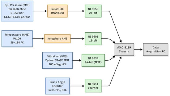
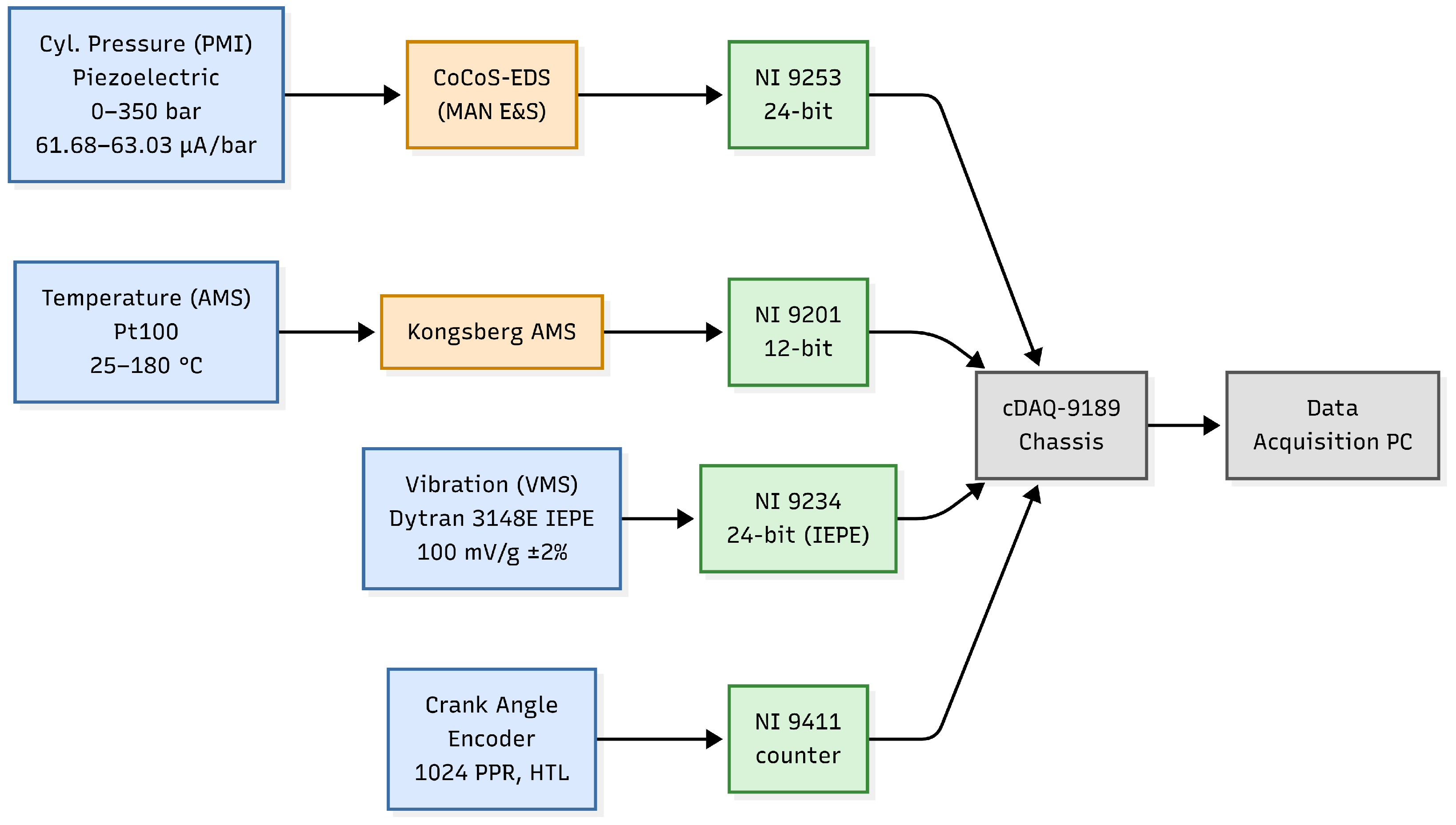
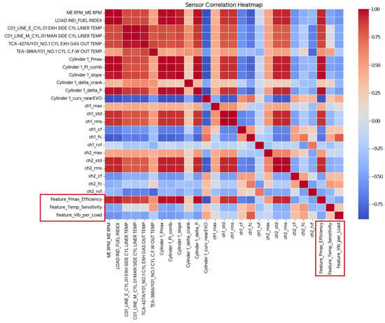
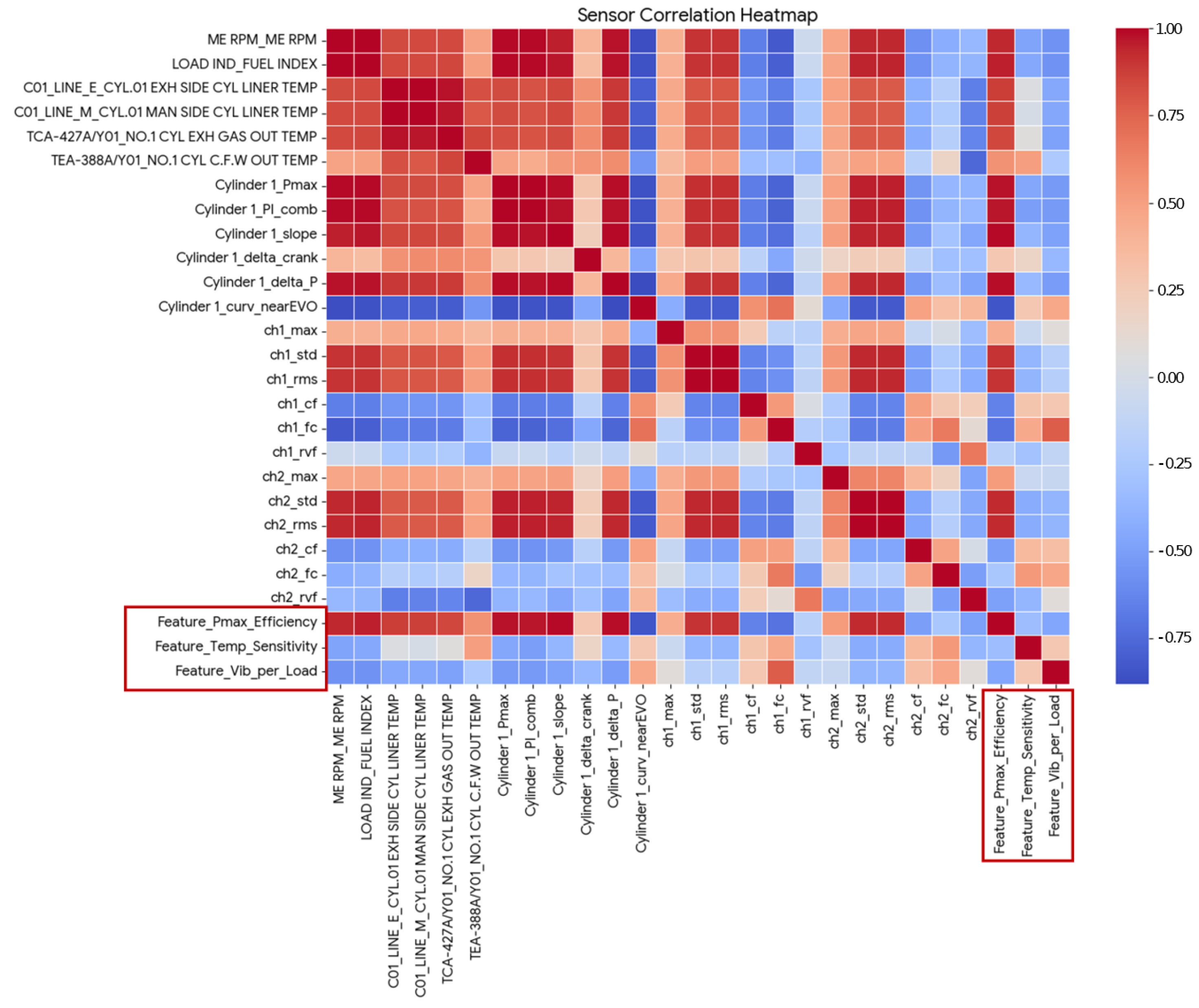
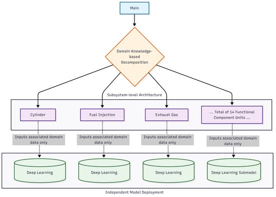
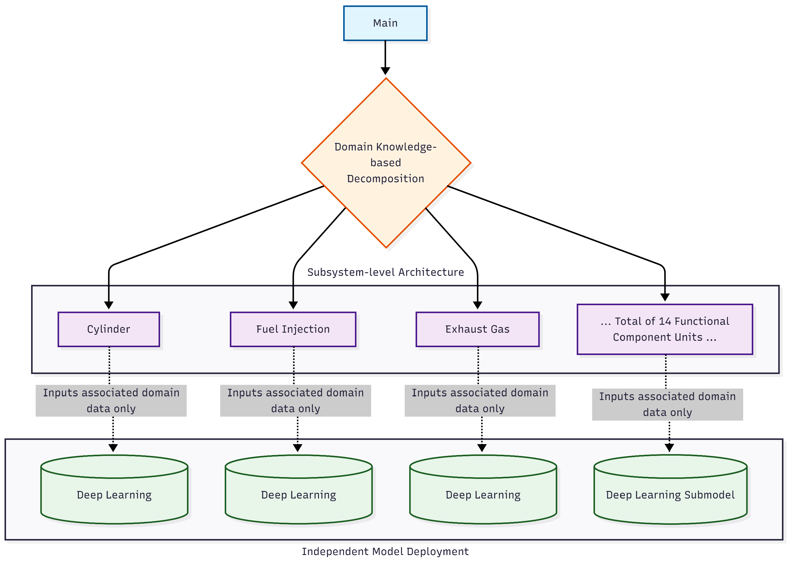
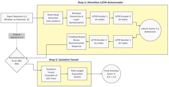
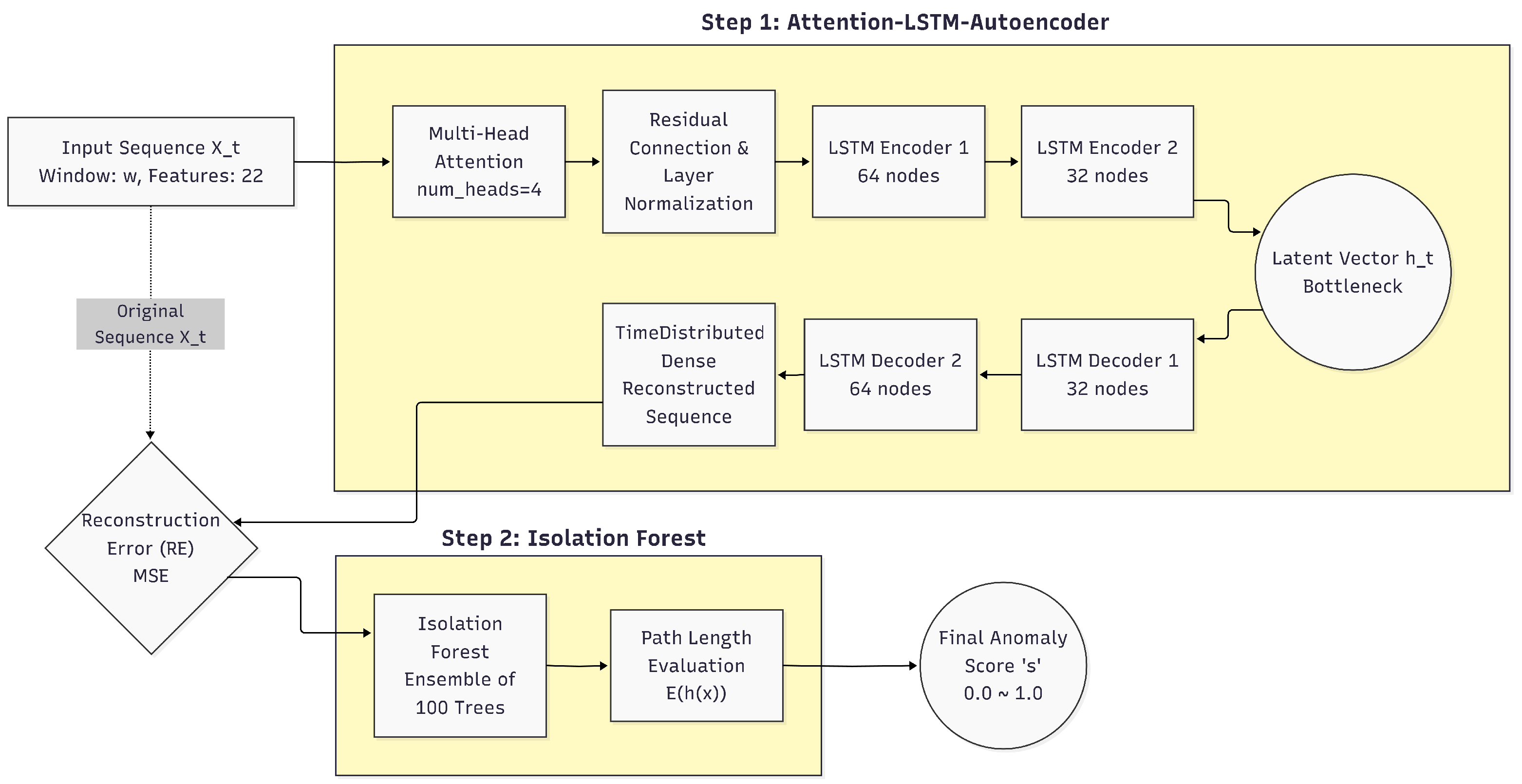
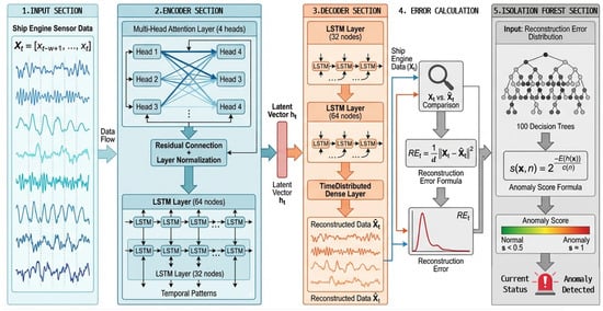
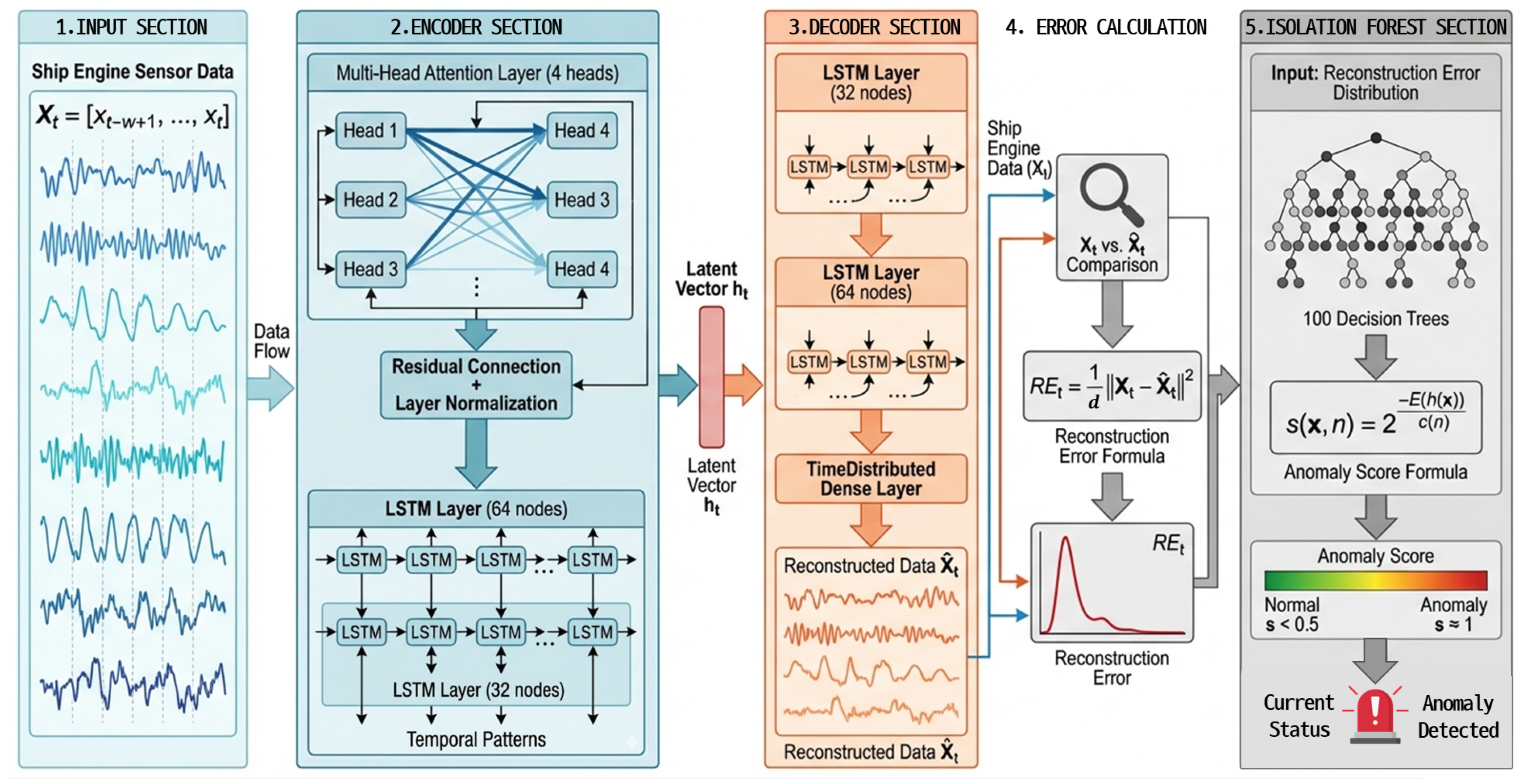
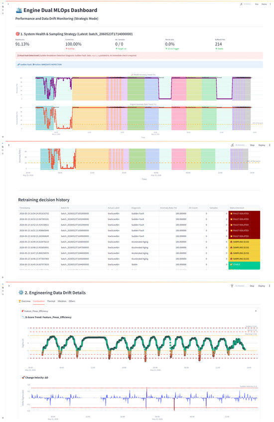
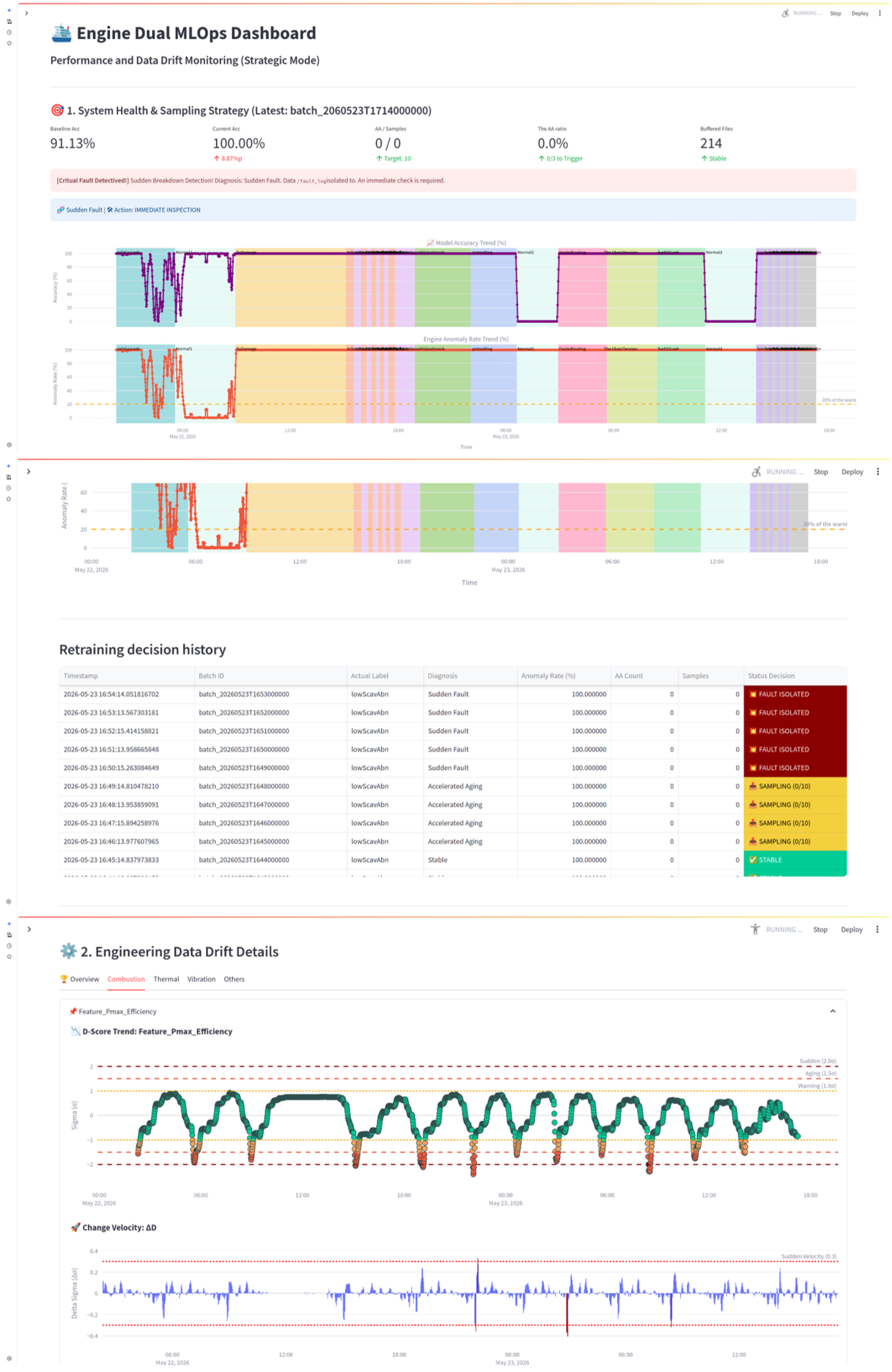
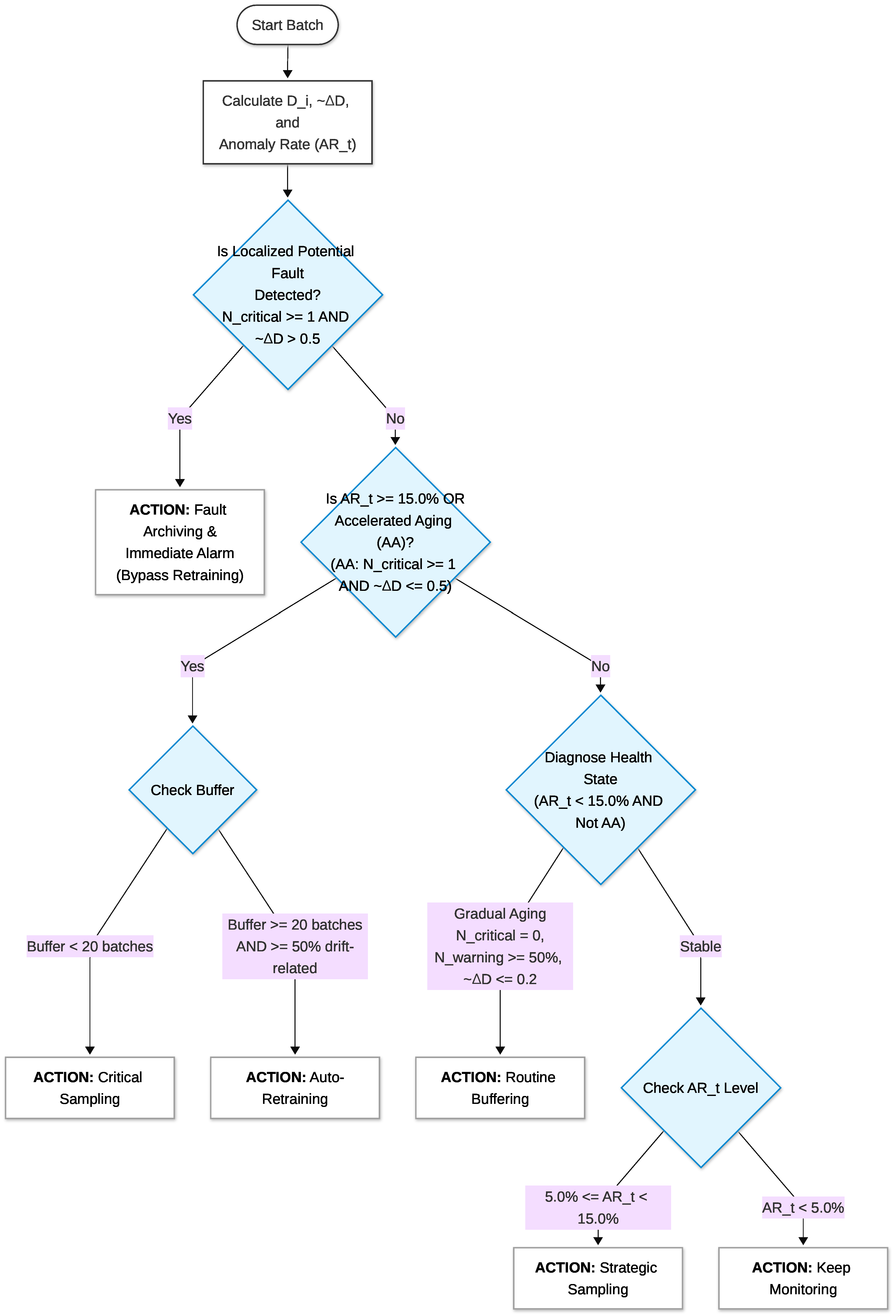
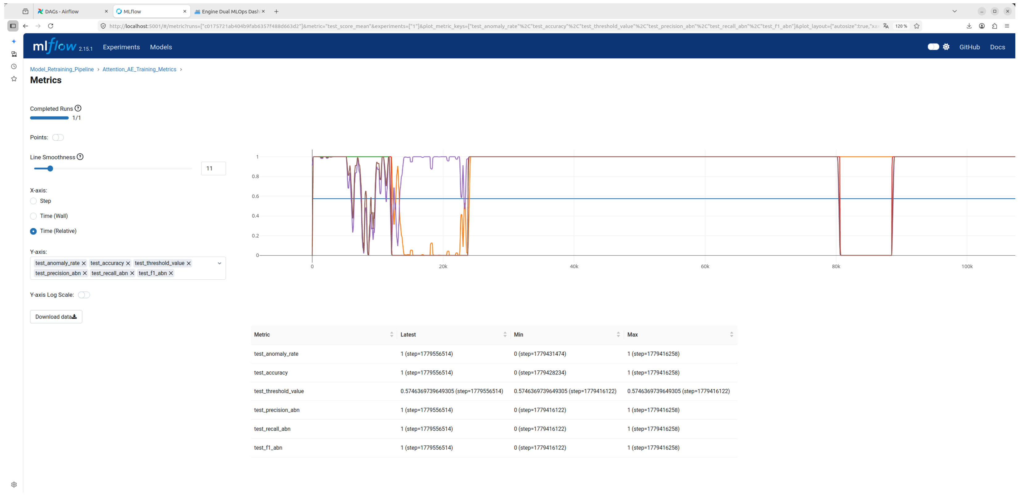
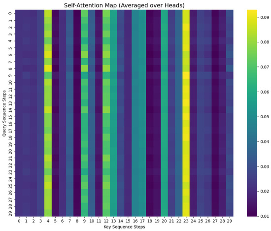
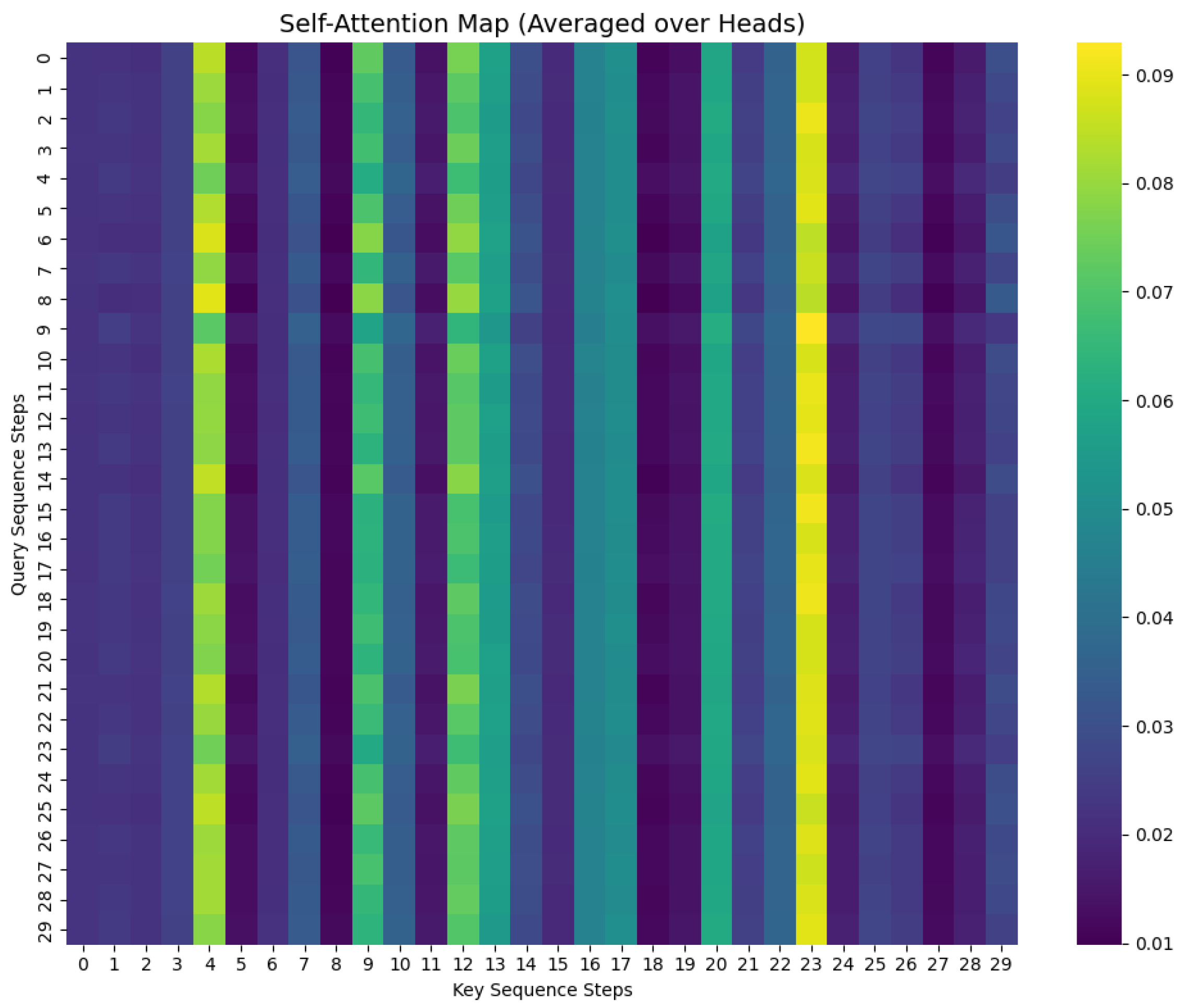
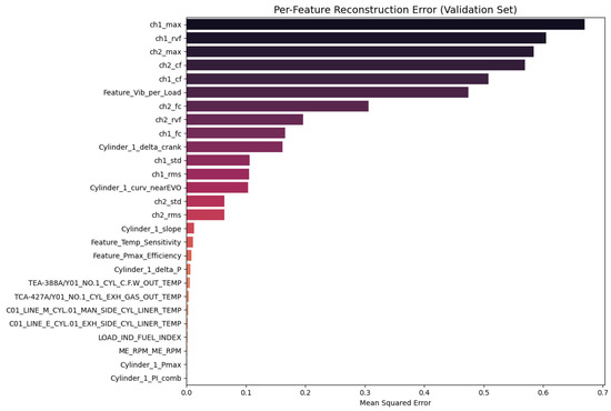
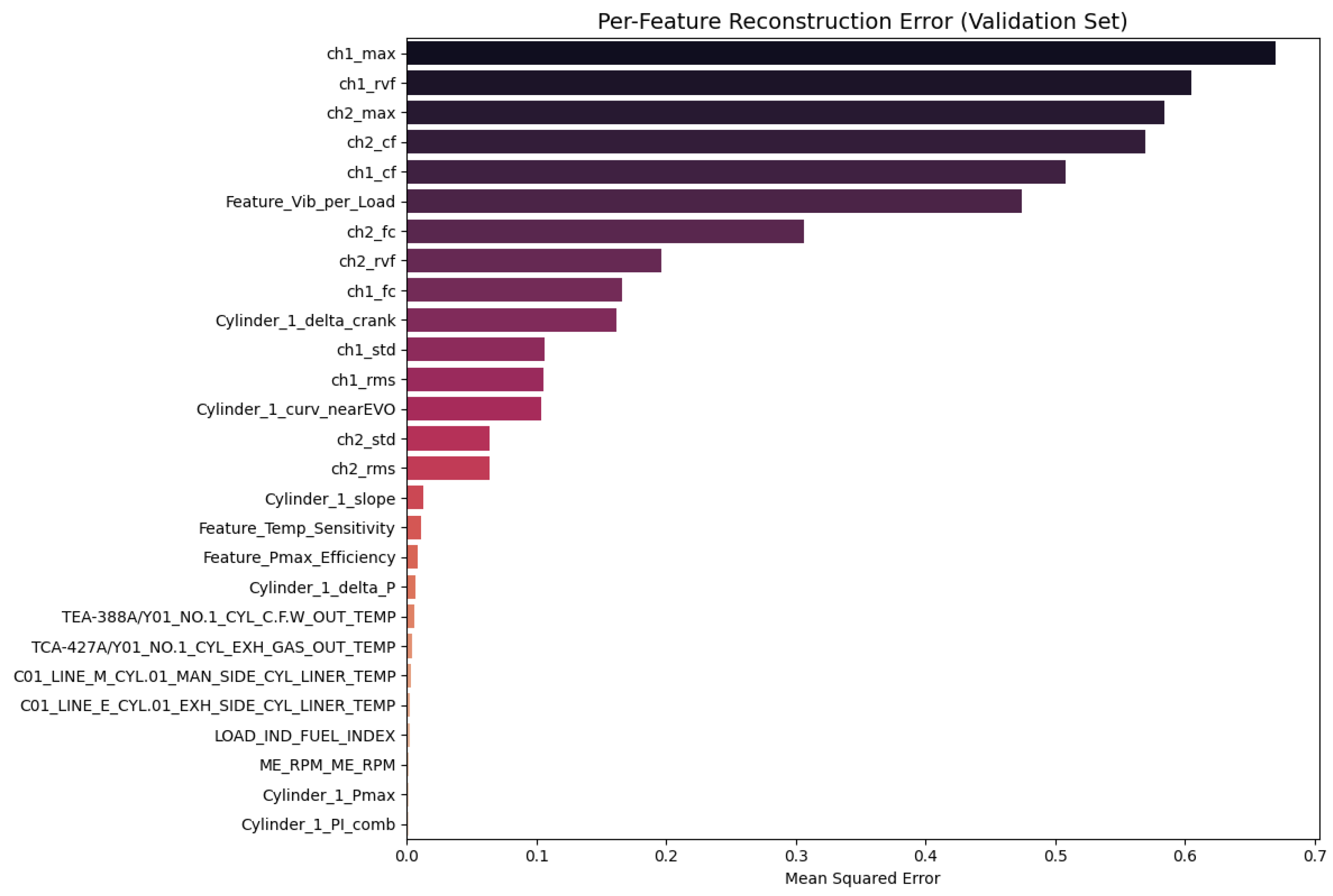
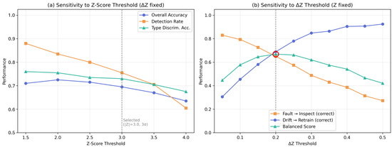
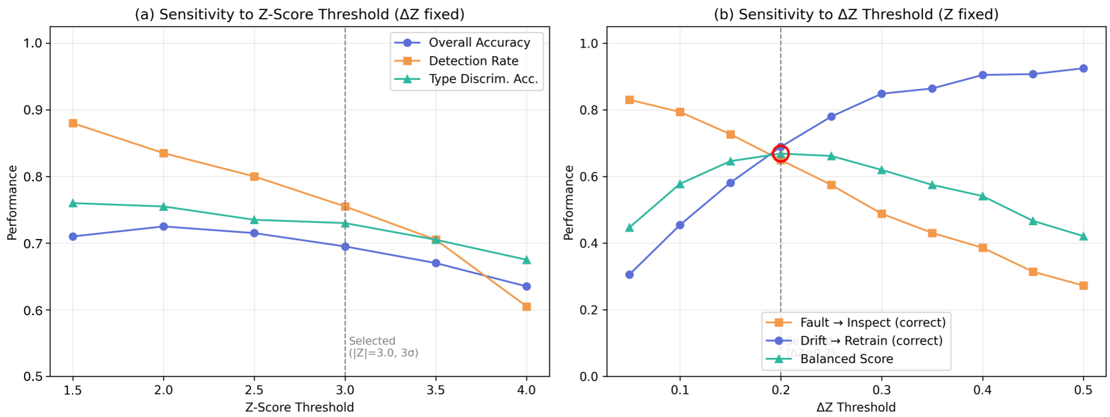
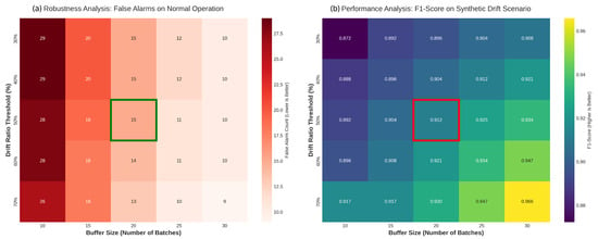
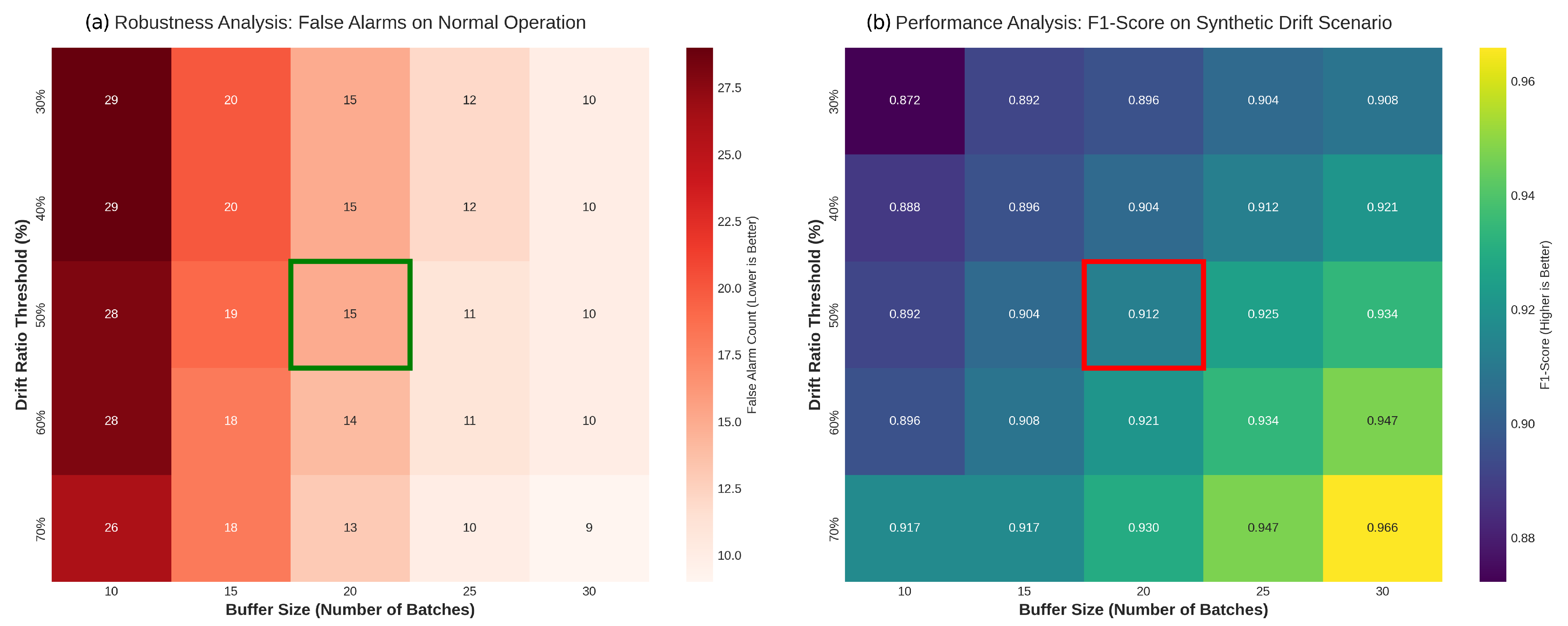
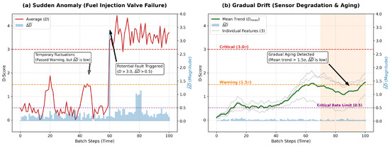
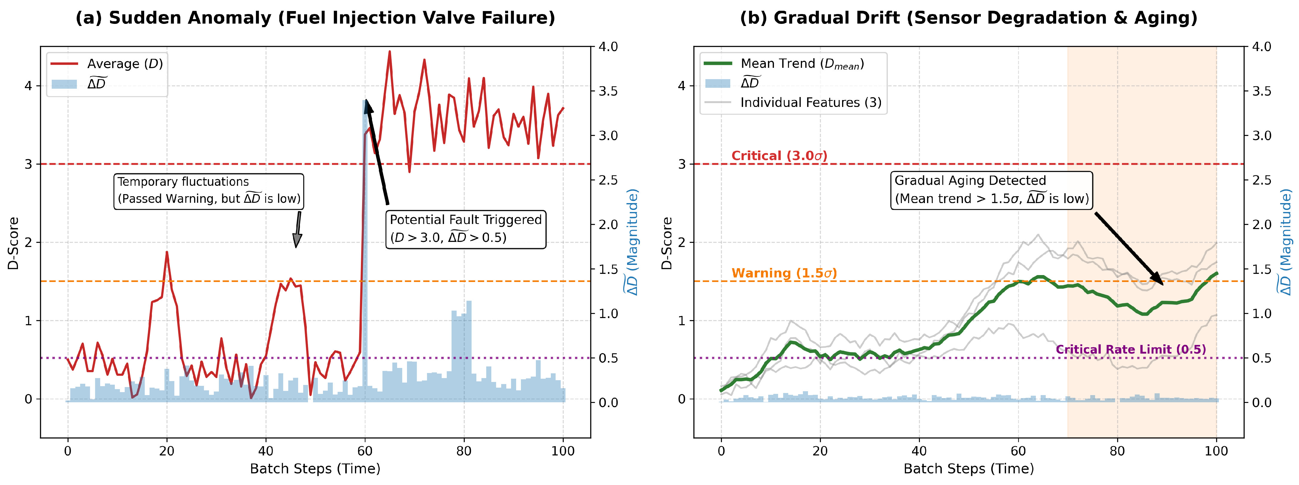
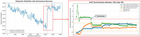
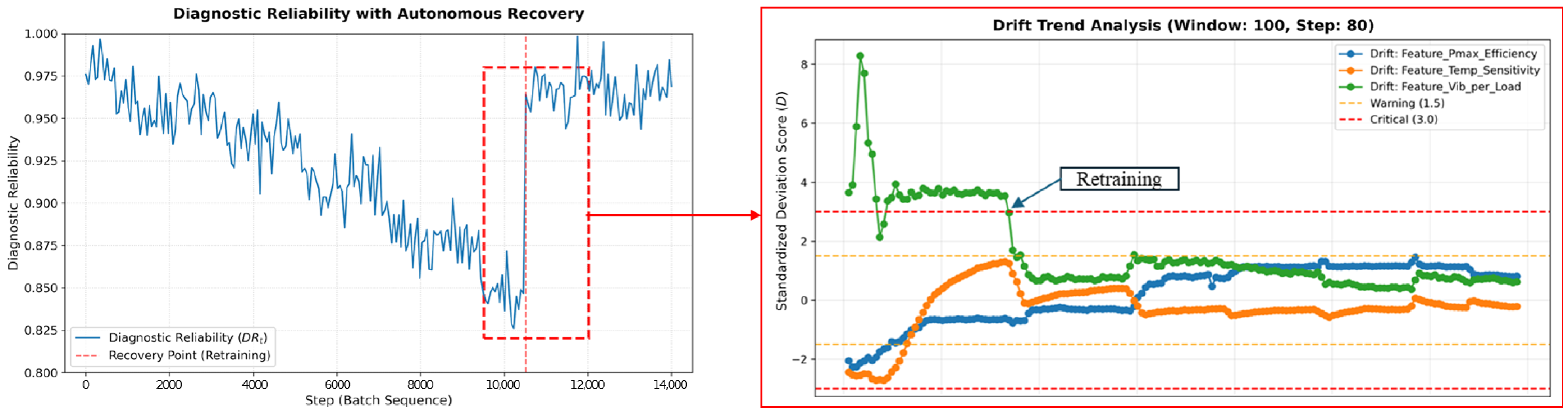

Disclaimer/Publisher’s Note: The statements, opinions and data contained in all publications are solely those of the individual author(s) and contributor(s) and not of MDPI and/or the editor(s). MDPI and/or the editor(s) disclaim responsibility for any injury to people or property resulting from any ideas, methods, instructions or products referred to in the content. |
© 2026 by the authors. Licensee MDPI, Basel, Switzerland. This article is an open access article distributed under the terms and conditions of the Creative Commons Attribution (CC BY) license.