


Abstract
Vessel traffic service systems in remote or newly established maritime regions face significant operational limitations due to the scarcity of historical AIS data, which undermines the reliability of trajectory-based situational awareness and collision risk assessment. Existing deep learning models, predominantly validated on data-rich major shipping corridors, suffer severe performance degradation under cross-domain deployment, rendering them impractical for vessel traffic management in underserved waters. To bridge this operational gap, this study proposes a Boundary-Aware Distillation and LoRA-Based Transfer (BD-LT) framework that enables reliable trajectory prediction with as few as 132 target-domain trajectories. The framework integrates HDBSCAN-based geographic-semantic domain partitioning, a Time-Aware Transformer with Time2Vec encoding for irregular AIS sampling, hybrid knowledge distillation with error-boundary gating for selective cross-domain transfer, and LoRA-based parameter-efficient adaptation to mitigate overfitting. Validated on NOAA full-scale AIS measurements, the framework reduces the 60 min Final Displacement Error by 35.2% relative to the no-framework baseline, consistently outperforming state-of-the-art models across all prediction horizons, with statistical reliability confirmed via bootstrap resampling. These results demonstrate the practical feasibility of deploying data-driven trajectory prediction in maritime regions where conventional approaches have historically been inapplicable, with direct implications for collision avoidance decision support and port approach traffic management.
1. Introduction
With the continued expansion of global maritime trade and the rapid development of intelligent shipping technologies, maritime traffic environments are becoming increasingly dense, dynamic, and operationally complex. This trend places growing demands on vessel traffic service (VTS), shore-based operators, and maritime decision-support tools. The Automatic Identification System (AIS) is a mandatory navigational system that continuously broadcasts static and dynamic vessel information, making it a primary data source for data-driven maritime surveillance and forecasting. AIS is required for all commercial vessels over 300 gross tonnage, all passenger ships regardless of size, and other vessels as mandated by international regulations, while smaller recreational ships are generally exempt. On this basis, vessel trajectory prediction has emerged as a key enabling technology for maritime situational awareness, collision avoidance support, and port traffic management [1,2,3]. Reliable multi-horizon prediction over 10 to 60 min is essential for proactive collision risk assessment, because it allows potentially hazardous encounters to be identified before vessels reach the closest point of approach, thereby creating time for intervention.
Research on vessel trajectory prediction has evolved substantially over the past decade. Early studies mainly relied on physics-based and kinematic approaches, such as Kalman filtering and related state-estimation methods, which model vessel motion through recursive equations and remain useful under relatively regular navigation conditions [4]. Traditional machine-learning methods, including support vector regression and Gaussian process models, later improved the ability to capture nonlinear motion patterns from AIS observations [5,6]. More recently, deep learning has become the dominant paradigm in this field. Recurrent neural networks such as LSTM and GRU have been widely applied to vessel trajectory forecasting because of their ability to model temporal dependencies in AIS sequences [7,8]. Hybrid architectures that combine convolutional and recurrent structures have further improved spatiotemporal feature extraction [9]. At the same time, Transformer-based and graph-based models have shown strong performance by better capturing long-range dependencies, interaction patterns, and multimodal future behaviors [10,11,12,13,14,15]. These advances have significantly improved prediction accuracy in data-rich maritime environments and have strengthened the role of trajectory prediction in maritime situational awareness.
However, despite this methodological progress, an important deployment gap remains. Most existing studies are developed and validated in major ports or heavily trafficked shipping corridors, such as Singapore, Rotterdam, or other high-density waterways, where large volumes of historical AIS data are available [3,12,16]. In contrast, many real-world maritime regions, including remote offshore routes, newly commissioned port approaches, and low-traffic regional waters, remain data-scarce. This imbalance is further illustrated in Figure 1, which compares vessel traffic density between a major hub port and a low-traffic regional port at the same spatial scale. It is operationally critical: such regions may still require collision risk monitoring and situational awareness support, yet conventional deep learning models often degrade sharply when transferred from data-rich source regions to geographically different target waters. Prior work has shown that differences in channel geometry, traffic organization, hydrological conditions, and local navigational rules can substantially reduce model generalization under cross-region deployment [17,18]. As a result, trajectory-based decision support remains effectively unavailable in many underserved maritime environments.
Figure 1.
AIS vessel traffic density at the same spatial scale for a major hub port and a low-traffic regional port. Source: NOAA Marine Cadastre AIS Vessel Traffic Data.
A second challenge lies in the irregular temporal nature of AIS reporting. In practice, AIS observations are not sampled at uniform intervals; reporting rates vary because of communication conditions, vessel maneuvering behavior, signal loss, and operational settings [19,20]. This irregularity is not merely a data-quality nuisance. The elapsed time between successive AIS reports contains motion-state information that is directly relevant to vessel inertia, maneuvering intent, and future path evolution. Nevertheless, many prediction pipelines still regularize AIS sequences through interpolation or resampling, implicitly assuming that temporal irregularity can be safely smoothed away [18]. An alternative view, increasingly supported by recent studies, is that irregular timing should be modeled explicitly rather than discarded, because it contains meaningful predictive structure and may improve robustness under real operational conditions [13,21]. This methodological divergence reflects a broader controversy in the field: whether prediction performance is better served by imposing uniform temporal structure for computational convenience, or by preserving the original timing information and learning from it directly.
A third unresolved issue concerns how knowledge from data-rich regions should be transferred to data-scarce regions. Two broad lines of research are relevant here: knowledge distillation and transfer learning. Knowledge distillation was originally proposed as a model-compression strategy in which a student network learns from a more capable teacher network through softened outputs or intermediate representations [22]. It has since been extended to sequence modeling, trajectory prediction, and traffic forecasting [23,24,25]. However, most existing distillation methods are developed for single-domain settings or assume that teacher and student data distributions are sufficiently aligned. This assumption becomes problematic in cross-region vessel trajectory prediction, where the source and target domains may differ substantially in geography and traffic semantics. In such cases, forcing the student to imitate the teacher indiscriminately may induce negative transfer rather than improve performance. Similarly, transfer learning has shown promise in maritime prediction tasks by transferring representations or physical priors from one domain to another [26,27]. Yet conventional pretrain–fine-tune strategies often require many trainable parameters and can easily overfit when target-domain data are extremely limited. Recent parameter-efficient fine-tuning methods, especially Low-Rank Adaptation (LoRA), suggest a different hypothesis: instead of fully updating a large pretrained model, it may be more effective to preserve general knowledge in the backbone and adapt only a small number of low-rank parameters [28]. This creates another divergence in the literature between full-parameter adaptation and parameter-efficient transfer, particularly under few-shot maritime conditions.
Taken together, these gaps indicate that the central problem is no longer simply how to maximize prediction accuracy in a single well-sampled region, but how to enable reliable trajectory prediction in maritime regions where data are scarce, sampling is irregular, and distribution shift is severe. Addressing this problem is important not only from a methodological perspective but also from an operational one. If trajectory-based situational awareness tools cannot be deployed outside a few major ports, then a large proportion of global maritime traffic remains beyond the reach of data-driven collision risk support.
To address this challenge, this study proposes a Boundary-Aware Distillation and LoRA-Based Transfer (BD-LT) framework for vessel trajectory prediction in data-scarce maritime regions.
The key technical contributions of this study are threefold. First, we formulate vessel trajectory prediction in data-scarce waters as a cross-region transfer learning problem and introduce an HDBSCAN-based geographic-semantic partitioning strategy to construct source and target domains with explicit spatial separation. This design moves beyond conventional random data splitting and provides a more realistic evaluation setting for deployment in low-traffic maritime regions. Second, we develop a Time-Aware Transformer backbone that incorporates Time2Vec-based temporal encoding to explicitly model irregular AIS sampling intervals and periodic navigation patterns. This enables the model to preserve temporal information that is often lost during interpolation or uniform resampling. Third, we propose a Boundary-Aware Distillation and LoRA-Based Transfer framework that combines selective teacher–student distillation with parameter-efficient target-domain adaptation. The boundary-aware gating mechanism reduces negative transfer by activating distillation only when the teacher provides a meaningful advantage, while LoRA-based adaptation mitigates overfitting by updating only low-rank adapter parameters in the data-scarce target domain.
The main findings of this study support the effectiveness of this approach. Using full-scale NOAA AIS data, the proposed framework enables reliable target-domain prediction with as few as 132 trajectories and reduces the 60 min Final Displacement Error by 35.2% relative to the no-framework baseline. It also consistently outperforms several representative baseline models across multiple prediction horizons, while bootstrap resampling confirms the statistical reliability of the observed gains. These results suggest that the long-standing exclusion of low-traffic and emerging maritime regions from data-driven trajectory prediction is not an inherent limitation of learning-based methods, but rather a consequence of insufficient mechanisms for modeling temporal irregularity, handling domain shift, and adapting under extreme data scarcity.
2. Methodology
This chapter presents the methodological framework developed in this study, with emphasis on the mathematical formulation and implementation of each component. To address the operational challenges posed by extreme maritime data imbalance and weak cross-region generalization, we propose the BD-LT framework for vessel trajectory prediction, aimed at extending trajectory-based maritime situational awareness and collision risk assessment to data-scarce waters (Figure 2). The overall pipeline consists of three tightly connected stages. First, a geographic-semantic clustering strategy is employed to partition AIS trajectories into source and target domains, thereby establishing a cross-region transfer setting. Second, a high-capacity teacher model is trained on the data-rich source domain, and its spatiotemporal knowledge is transferred to a lightweight student model through boundary-aware distillation. Finally, the distilled student model is adapted to the data-scarce target domain using LoRA-based low-rank transfer.As shown in the figure, the three different colored curves represent the prediction results for different possibilities. The red color represents the prediction trajectory with the highest likelihood, the green color is the prediction trajectory with the middle likelihood, and the blue color is the prediction trajectory with the lowest likelihood.
Figure 2.
Overall workflow of training and inference.
2.1. Data Preprocessing
2.1.1. Coordinate Transformation and Feature Extraction
Since geographic coordinates in the WGS84 system are subject to the effects of Earth’s curvature, their direct use for Euclidean distance computation and model training introduces distance distortion and feature degradation. Accordingly, all geographic coordinates are converted into a local East-North-Up (ENU) coordinate system. For a trajectory point at any time t, the positional displacement () relative to the trajectory origin at time is computed as follows:
where R ≈ 6371 km denotes the mean radius of the Earth, () represent the latitude and longitude (in radians) at time t, and () are the reference coordinates of the trajectory origin.
On this basis, the model input feature vector is constructed. Beyond positional displacement, kinematic features including velocity, acceleration, and rate of turn are extracted to explicitly model the physical constraints imposed by the large inertia of vessel mass [22]. Additionally, temporal encoding features are incorporated to capture the periodic patterns of maritime traffic flow along hourly and weekly dimensions [29]. The feature vector is formally defined as:
where denotes the normalized Speed Over Ground (SOG); represents the Course Over Ground (COG), encoded via sine and cosine functions to eliminate the discontinuity inherent in angular periodicity; is the approximate acceleration, derived from the finite difference in velocities at adjacent time steps; is the rate of turn, obtained from the finite difference in heading angles; and contains periodic sine/cosine positional encodings for hour-of-day and day-of-week, designed to capture the temporal regularity of maritime traffic.
2.1.2. Source and Target Domain Partitioning via Density-Based Clustering
To systematically characterize the imbalance in maritime data and establish a cross-domain evaluation scenario with well-defined geographic semantics, this paper proposes an automated domain-partitioning method based on trajectory origin clustering. Unlike conventional random splitting, clustering-based partitioning ensures complete geographic isolation between domains, compelling the model to learn transferable motion patterns rather than region-specific representations. By employing clustering-based partitioning, we ensure complete geographic isolation between the source and target domains, thereby compelling the model to learn universal motion patterns rather than region-specific local representations [30].
To more accurately measure the similarity between trajectory origins, we define a hybrid distance metric that integrates geographic location and motion state. For two trajectory origins and , the distance is computed as:
where = 0.7, = 0.15, and = 0.15 are the weighting coefficients for geographic distance, speed, and heading, respectively. and denote the normalized speed difference and angular difference, respectively. is calculated using the Haversine formula for spherical distance:
The Hierarchical Density-Based Spatial Clustering of Applications with Noise (HDBSCAN) algorithm is then applied to cluster all trajectory origins. This algorithm effectively identifies geographically coherent regions corresponding to ports or channel entry zones, while labeling outliers as noise.
After clustering, the number of valid trajectories within each cluster is tallied. To distinguish data-rich regions from data-scarce ones, the mean trajectory count across all clusters is computed as the partitioning threshold. Based on this threshold, each cluster is assigned to either the source domain set or the target domain set :
Through the above procedure, busy ports with above-average trajectory counts are designated as the source domain for training the teacher model, while data-scarce regions are designated as the target domain, serving as the test scenario for evaluating model transferability.
2.2. Boundary-Aware Distillation and LoRA-Based Transfer Framework
The proposed Boundary-Aware Distillation and LoRA-Based Transfer (BD-LT) framework is a hybrid learning framework that combines knowledge distillation and parameter-efficient transfer learning. In terms of methodological classification, knowledge distillation belongs to a teacher–student learning paradigm, in which a compact or target-oriented student model learns not only from ground-truth trajectory labels but also from the prediction behavior and intermediate representations of a stronger teacher model. LoRA-based transfer learning, by contrast, belongs to the category of parameter-efficient fine-tuning methods. Instead of updating all parameters of the pretrained model, it freezes the main backbone and introduces a small number of trainable low-rank adaptation matrices, thereby reducing overfitting risk under data-scarce target-domain conditions.
In this study, BD-LT is designed for cross-region vessel trajectory prediction, where the source domain contains abundant AIS trajectories and the target domain contains only limited local data. The framework is implemented through three sequential steps. First, a high-capacity teacher network is trained on the data-rich source domain to learn general spatiotemporal vessel motion patterns. Second, a lightweight student network is trained through boundary-aware knowledge distillation, where the student receives supervision from both the ground-truth labels and the teacher model. The distillation signal is selectively activated for samples where the teacher provides a meaningful advantage, thereby reducing the risk of negative transfer. Third, the distilled student network is adapted to the data-scarce target domain using LoRA-based low-rank fine-tuning. During this stage, the backbone parameters are frozen, and only the injected low-rank adapters are updated, allowing the model to fit target-domain characteristics while preserving the transferable knowledge learned from the source domain.
Therefore, the proposed BD-LT framework can be regarded as a teacher–student distillation framework followed by parameter-efficient domain adaptation. This design enables the model to first acquire transferable motion knowledge from data-rich waters and then adapt this knowledge to data-scarce maritime regions with limited trainable parameters.
This study devises a two-stage learning paradigm of BD-LT, whose overall architecture is illustrated in Figure 3. The BD-LT framework operates in two sequential stages. In the first stage, a teacher network is fully trained on the data-rich source domain, and its knowledge is transferred to a lightweight student network through boundary-aware distillation. In the second stage, the distilled student is adapted to the data-scarce target domain via LoRA-based low-rank fine-tuning. The three core components of this pipeline—the Time-Aware Transformer backbone, the boundary-aware distillation mechanism, and the LoRA transfer module—are detailed in the following subsections.
Figure 3.
BD-LT framework diagram.
2.2.1. Time-Aware Transformer Model
Conventional Transformers rely on sinusoidal positional encoding to mark the relative positions of elements within a sequence. However, the sampling interval of AIS data exhibits considerable randomness (ranging from a few seconds to several minutes), and index-based positional encoding alone cannot reflect the true physical passage of time or motion inertia. To address this, the present study introduces a Time2Vec module to construct continuous temporal representations.
Time2Vec maps a scalar time input (in this study, the time interval between adjacent observations) to a vector of length k + 1. This mapping comprises two core components: a linear term that captures aperiodic trends and sinusoidal terms that capture periodic patterns. Its mathematical formulation is as follows:
where denotes the input time interval, and and are learnable frequency and phase parameters, respectively. When , the linear term captures features that vary monotonically with time (e.g., the cumulative positional drift of a vessel over long intervals), enabling the model to perceive the physical principle that the longer the elapsed time, the greater the state changes. When , the periodic terms capture latent local periodic patterns, enhancing the model’s capacity to fit complex temporal dynamics.
The final input embedding vector is composed of the trajectory feature projection, Time2Vec temporal embedding, and macroscale periodic encoding:
where denotes geometric features (e.g., changes in latitude and longitude, speed); is the absolute temporal positional encoding of each observation relative to the trajectory origin; and represents hour-of-day and day-of-week features encoded via sine and cosine functions, which introduce macroscale periodicity priors inherent to maritime traffic.
After obtaining the embedding vector enriched with spatiotemporal semantics, the data enter the Transformer encoder for deep feature interaction. This study adopts a 4-layer stacked architecture, each layer consisting of two principal sub-layers: multi-head self-attention and a position-wise feed-forward network.
The self-attention mechanism dynamically aggregates contextual information by computing correlations among different observations in the sequence. For an input sequence , it is first linearly projected into query (Q), key (K), and value (V) matrices:
Subsequently, scaled dot-product attention is used to compute weights and perform weighted summation:
To prevent the model from exploiting future information, a masking mechanism is applied during attention score computation, setting the association weights for future time steps to . The multi-head mechanism partitions the input into h = 4 independent heads computed in parallel, enabling the capture of diverse motion patterns from different representational subspaces.
The output of each attention layer passes through residual connections and layer normalization before entering the feed-forward network. The FFN consists of two linear transformations with an intermediate activation function, enhancing the nonlinear feature transformation capacity:
In the configuration adopted in this study, the Transformer hidden dimension is set to 128, the FFN expansion factor is set to 4 (yielding an intermediate dimension of 512), and a dropout rate of 0.1 is applied to prevent overfitting.
2.2.2. Boundary-Aware Distillation Mechanism
Knowledge distillation is used here as a teacher–student knowledge transfer strategy. The teacher network, trained on the source domain, usually has stronger representation capacity because it learns from a much larger number of trajectories. The student network is expected to inherit this source-domain motion knowledge while maintaining a more compact and target-adaptable structure. Unlike ordinary supervised learning, where the model learns only from ground-truth labels, knowledge distillation introduces additional supervision from the teacher model, including intermediate features and softened output distributions.
In the first stage, the student network learns from the teacher network through distillation on the source domain. To align the feature spaces, we introduce Hint Distillation, which encourages the intermediate-layer representations of the student network to mimic those of the teacher network. Specifically, let the output features of the teacher and student at the lll-th layer be denoted by and , respectively, where B is the batch size, L is the sequence length, and D is the feature dimension. To extract global contextual information, we first apply a learnable weight allocation mechanism to automatically identify the importance of each dimension in the sequence and then perform attention-based pooling on the feature vectors through weighted summation to obtain the global representations and . These representations are subsequently aligned by minimizing the mean squared error (MSE).
To prevent the student model from being forced to imitate potentially unreliable teacher predictions in the target domain, we design a boundary-aware distillation mechanism that introduces a dynamic gating strategy based on the performance gap between the teacher and the student. For each sample, the prediction errors of both the student and teacher models are computed. The distillation loss is activated only when the student performs substantially worse than the teacher, namely, when the performance gap exceeds a dynamic threshold. In this study, the threshold factor is set to 0.2, corresponding to the hyperparameter delta_ratio. Once activated, the distillation loss is formulated as a temperature-scaled Kullback–Leibler (KL) divergence:
where and denote the logit outputs of the teacher and student at prediction horizon h, respectively; is the Softmax function; and is the distillation temperature coefficient, set to 4 in this paper. The final total training loss is a weighted combination of the task loss , the Hint loss, and the gated KD loss, with weights in the ratio 1.0:0.5:1.0.
2.2.3. LoRA-Based Target-Domain Transfer Mechanism
In this study, the LoRA-based transfer stage is conducted under a data-scarce target-domain setting. After the student network has acquired source-domain knowledge through boundary-aware distillation, it is transferred to the target domain, which contains only 132 trajectories in total and 105 trajectories for training. This setting is intentionally designed to simulate maritime regions where only limited historical AIS data are available. Under such conditions, full-parameter fine-tuning may easily overfit the small target-domain training set and damage the source-domain representations learned during distillation.
To address this issue, the backbone parameters of the distilled student model are frozen during target-domain adaptation. LoRA adapters are inserted only into selected Transformer layers, and only the low-rank matrices in these adapters are updated. Specifically, LoRA is applied to the query projection, value projection, and feed-forward network layers of the Transformer encoder. These modules are selected because the query and value projections directly influence attention-based temporal dependency modeling, while the feed-forward layers control nonlinear feature transformation. By adapting these components, the model can adjust to target-domain navigation patterns without updating the entire backbone.
LoRA-based transfer learning is adopted as a parameter-efficient domain adaptation strategy. In conventional full-parameter fine-tuning, all parameters of the pretrained student model are updated on the target-domain data. However, when the target domain contains only a small number of trajectories, such full-parameter adaptation may destroy the source-domain representations learned through distillation and lead to overfitting or catastrophic forgetting. To avoid this problem, LoRA freezes the original backbone parameters and introduces trainable low-rank matrices into selected layers. In this way, the model adapts to the target domain through a small number of additional parameters while preserving the distilled source-domain knowledge.
The backbone parameters of the student network, which carry the distilled dark knowledge, are treated as non-volatile memory units and completely frozen, excluding them from gradient updates. To endow the model with the capacity to adapt to new maritime regions, pairs of trainable low-rank matrices are injected as bypasses into the self-attention output projections and FFN linear layers of the last two Transformer encoder layers.
Let x denote the input to a given layer. The corrected output h after LoRA injection is computed as:
where is the down-projection matrix (initialized with a Gaussian distribution), is the up-projection matrix (initialized to zero), is the rank (set to in this study, satisfying ), and is a scaling hyperparameter. This low-rank decomposition ensures that the output at the initial stage of training remains consistent with the pretrained state. Subsequently, only A and B are updated via gradient descent, thereby reconstructing the target-domain feature mapping with a parameter overhead of merely 1–2%.
The rank r controls the dimension of the low-rank update and therefore determines the adaptation capacity of the LoRA module. A smaller r introduces fewer trainable parameters and provides stronger regularization but may limit the ability to fit target-domain characteristics. A larger r increases the expressive capacity of the adapter but may also increase the risk of overfitting when the target-domain sample size is extremely small. The scaling factor alpha controls the magnitude of the LoRA update relative to the frozen backbone output. A larger alpha strengthens the influence of the adapter, whereas a smaller alpha keeps the adapted model closer to the distilled source-domain representation. Therefore, r and alpha jointly determine the balance between target-domain adaptability and source-domain knowledge preservation.
Through the parameter isolation afforded by LoRA and the replay constraint from source-domain data, the framework effectively strikes an optimal balance between preserving distilled source-domain knowledge and fitting the target-domain distribution, thereby resolving the overfitting challenge under few-shot conditions.
2.3. Prediction Module
To address the inherent uncertainty in maritime navigation, this study designs a decoder comprising an attentive pooling mechanism and a dual-stream calibration architecture, termed the multi-horizon multi-modal prediction head. As illustrated in Figure 4, this module is designed to generate K potential navigational trajectories in parallel, along with their corresponding confidence probabilities for different prediction horizons.
Figure 4.
Architecture diagram of the trajectory prediction module.
Let the hidden state sequence output by the encoder be , where is the historical sequence length and is the feature dimension. To compress the temporal features into a global context vector for future prediction, an attentive pooling layer is first applied:
where denotes the normalized attention score computed through learnable weights. The global vector is then fed into a shared Multi-Layer Perceptron (MLP) for feature reorganization, extracting high-order semantic representations for downstream branches.
To simultaneously capture both the spatial trajectory positions and the intent probabilities of vessel motion, the prediction head adopts a dual-stream architecture responsible for trajectory generation and probability estimation, respectively. For each prediction horizon minutes, the model outputs 3 modes.
The trajectory generation branch aims to predict spatial positional displacements under different latent intents. Through a linear mapping layer , the branch directly regresses the two-dimensional coordinate increments of 3 candidate trajectories:
The absolute geographic coordinates of the k mode at the predicted time step are computed as:
where is the terminal point of the historical trajectory. This design enables the model to infer multiple feasible future paths based on the current motion inertia.
The probability estimation branch outputs raw log-probability logits and applies a cascaded dual-stage calibration to correct overconfidence. In the first stage, a learnable temperature parameter rr r smooths the logit distribution:
When , the distribution becomes flatter, encouraging exploration of low-probability modes; when , it sharpens toward high-confidence modes. In the second stage, a variance scaling factor σ\sigma σ derived from the model’s predicted covariance applies a secondary penalty to high-uncertainty modes:
This two-stage design ensures that high-variance prediction modes are appropriately down-weighted before the final Softmax normalization:
The rationale for dual-stage rather than single-stage calibration is that temperature scaling alone adjusts distributional entropy globally, whereas variance scaling introduces a sample-level penalty proportional to predicted uncertainty—a distinction that proves consequential when modal confidence distributions shift substantially across prediction horizons.
2.4. Evaluation Metrics
To comprehensively assess the geometric accuracy and probabilistic reliability of the model over different prediction ranges, a set of multidimensional quantitative metrics was used in this study. The evaluation covers three prediction horizons: 10, 30, and 60 min. These horizons were selected to provide a coarse-grained multi-scale assessment of the proposed framework under short-, medium-, and long-range forecasting conditions. We acknowledge that finer-grained short- to medium-term intervals, such as 6, 12, 18, and 24 min, are also commonly used in maritime trajectory prediction and collision-risk assessment. Compared with such uniformly spaced intervals, the 10/30/60 min setting is intended to evaluate not only near-term motion continuity but also medium-term route evolution and long-horizon error accumulation.
Specifically, the 10 min horizon represents short-term motion prediction, where the future position is still strongly constrained by the vessel’s current speed, heading, and inertia. The 30 min horizon is used as a medium-term forecasting point, comparable in scale to the commonly used 24 min interval but slightly extended to better capture route evolution and turning behavior. The 60 min horizon further evaluates long-range prediction stability, cumulative error growth, and cross-region generalization, which are particularly relevant to VTS-level situational awareness and early risk screening in data-scarce maritime regions. Therefore, the selected horizons are not intended to replace the 6/12/18/24 min setting, but to provide a complementary multi-scale evaluation focused on short-, medium-, and long-horizon generalization.
ADE quantifies the average positional deviation between the predicted trajectory and the ground truth trajectory across all intermediate time steps within the prediction window. By computing the mean Euclidean distance over the full prediction horizon, ADE provides a holistic assessment of trajectory-level fitting quality, capturing the degree to which the model successfully reconstructs the spatial evolution of vessel motion. Unlike endpoint-focused metrics, ADE penalizes accumulated positional drift across the entire prediction sequence, making it sensitive to systematic bias in the model’s representation of motion dynamics. For a given prediction horizon , it is computed as:
where denotes the Euclidean norm, representing the geographic straight-line distance between two points.
From a practical standpoint, ADE serves as the primary indicator for evaluating whether the proposed BD-LT framework preserves temporal coherence across the full prediction sequence. In the context of vessel trajectory prediction, a low ADE value implies that the model consistently approximates the vessel’s motion throughout the entire prediction window, rather than merely arriving at a correct endpoint by chance. A model with low ADE but high FDE would exhibit well-controlled intermediate-step errors yet diverge sharply at the prediction horizon, whereas a model with low FDE but high ADE would converge to the correct endpoint through an erroneous path, both of which are operationally undesirable for maritime situational awareness. In this study, ADE is evaluated across three prediction horizons (10, 30, and 60 min) and functions as the principal basis for comparing the long-horizon trajectory fitting quality among baseline architectures under both source-domain and target-domain settings, thereby providing a systematic characterization of how each model’s trajectory-level accuracy evolves as the prediction window extends.
FDE measures the Euclidean distance between the predicted position and the true position exclusively at the final time step of the prediction horizon, thereby isolating the model’s ability to correctly forecast the terminal state of the vessel. In contrast to ADE, which distributes the error signal uniformly across all intermediate prediction steps, FDE concentrates evaluation on the endpoint, making it a particularly discriminative indicator for assessing long-range predictive accuracy. This endpoint-centric perspective is not merely a methodological choice but carries direct operational significance in the maritime domain: accurate final-position prediction is the foundational prerequisite for estimating the Closest Point of Approach (CPA) between vessels, a quantity that serves as the primary quantitative basis for collision risk assessment and proactive intervention decision-making. FDE thus represents the tightest coupling between model performance and operational utility in the context of this study. FDE is calculated as:
To compensate for the limitation of ADE in penalizing large error samples, RMSE is introduced as a supplementary metric, which is more sensitive to outliers and can effectively quantify the robustness of the model under extreme operating conditions. Similar to ADE, this metric is also calculated based on the Top-1 prediction model, and its mathematical definition is as follows:
The quadratic amplification inherent to RMSE means that a small number of high-error prediction instances can disproportionately elevate the aggregate score, exposing structural vulnerabilities that ADE, with its linear averaging, may otherwise obscure. A lower RMSE value thus indicates not only that the model achieves satisfactory average-case accuracy, but also that it maintains well-controlled maximum deviations when confronted with complex trajectory perturbations, reflecting genuine robustness rather than merely favorable mean performance.
3. Experiment
3.1. Experimental Setup
All experiments are conducted on a high-performance computing platform. The hardware configuration is detailed in Table 1. Model training was primarily performed on NVIDIA GeForce RTX 4090D and Quadro RTX 8000 GPUs, while lightweight inference tests were carried out on an NVIDIA GeForce RTX 4060.
Table 1.
Experimental environment configuration.
3.2. Dataset
The Automatic Identification System (AIS) data used in this study are sourced from the Marine Cadastre database provided by the National Oceanic and Atmospheric Administration (NOAA) (https://marinecadastre.gov/accessais/, accessed on 20 August 2025). This dataset covers coastal waters with extensive shipping activity and contains both dynamic and static vessel information. The raw AIS files are originally in SPNMEA format; for this study, we used the cleaned CSV files provided by NOAA, which already include key fields such as MMSI (Maritime Mobile Service Identity), timestamp, longitude, latitude, Speed Over Ground (SOG), and Course Over Ground (COG), totaling 19,549 trajectories.
To ensure data quality, we further removed anomalous records that contained physically implausible values (e.g., SOG > 60 knots, missing or invalid coordinates) or trajectories that were excessively short in duration or length. Following this preprocessing pipeline, 14,811 trajectories remained, grouped into 128 origin clusters. Each origin cluster contains an average of 115 trajectories. Figure 5 presents a bubble map of the spatial distribution of trajectory starting points. Each bubble represents a geographic region centered on the starting location of a trajectory cluster, where the bubble size reflects the number of trajectories associated with that region. To facilitate source–target domain partitioning, the regions are further divided according to a trajectory-count threshold of 115: regions with more than 115 trajectories are marked in blue, while those with fewer than 115 trajectories are marked in red. As shown in the figure, high-density regions are mainly concentrated along major shipping areas on the east and west coasts of North America, whereas relatively sparse regions are scattered across several peripheral and offshore waters. This spatial heterogeneity provides the empirical basis for distinguishing data-rich source-domain regions from data-scarce target-domain regions.
Figure 5.
Bubble plot of the distribution of the starting cluster of the trajectory.
Using the mean trajectory count per origin cluster as the partitioning criterion, the origin clusters and their constituent trajectories are divided into target and source domains. The post-partitioning trajectory distribution is illustrated in Figure 6, which visually presents the geographic coverage of vessel trajectory data in North American waters and the stark quantitative disparity between the source and target domains. At a macroscopic level, the source domain data (blue, 14,679 trajectories) form an extensive traffic network spanning the East and West Coasts as well as the major shipping lanes of the Gulf of Mexico, exhibiting exceptionally high spatial coverage and connectivity. In contrast, the target domain data (red, 132 trajectories) appear only as sporadic fragments scattered across specific waters. Together with Figure 5 and Figure 6, these results reveal that the target domain data are not only scarce in quantity but also exhibit significant domain discrepancy from the source domain in terms of spatial distribution characteristics.
Figure 6.
Spatial distribution of source domain trajectories in the target domain.
On this basis, the source and target domains are each split into training, validation, and test sets at an 8:1:1 ratio. The trajectory counts within each partition are presented in Table 2.
Table 2.
Distribution of the number of trajectories in the source domain and target domain.
It should be noted that the source and target domains are derived from geographically separated subsets of the same NOAA AIS database rather than from two fully independent datasets. This design is intentional because the purpose of this study is to evaluate cross-region transfer under a controlled data source while avoiding confounding effects caused by different data providers, collection standards, or preprocessing pipelines. The HDBSCAN-based partitioning ensures that the source and target domains are not randomly mixed but correspond to spatially distinct trajectory clusters with different traffic densities. Therefore, the experimental setting should be interpreted as a controlled cross-region transfer scenario within a unified AIS data source.
3.3. Sensitivity Analysis
The framework proposed in this study involves multiple critical hyperparameters across the distillation stage and the LoRA transfer stage, whose values directly influence the model’s final performance on the data-scarce target domain. To verify the rationality of each core hyperparameter selection and identify the optimal configuration, this section conducts systematic sensitivity experiments on the LoRA rank parameter rrr and scaling factor α\alphaα, as well as the boundary ratio delta_ratio in the boundary-aware distillation stage. All experiments use FDE at 60 (nmi) as the evaluation metric and are trained for 5 epochs. The student network is evaluated on the target domain validation set, while the teacher network is evaluated on the source domain validation set.
Figure 7 presents the FDE at 60 variation curves for the boundary control parameter delta_ratio across 10 values in {0.1, 0.2, 0.3, 0.4, 0.5, 0.6, 0.7, 0.8, 0.9}. The influence of delta_ratio on model performance is highly pronounced, with the curve exhibiting a distinct U-shaped trend. The optimum occurs at 0.2, and the FDE at 60 variation spans 1.19 nmi. When this parameter deviates from the optimum in either direction, performance degrades substantially. In the right interval, an excessively high gating threshold means that only a very small number of high-error samples are subjected to the distillation constraint, resulting in overly narrow coverage of the distillation signal; consequently, the student network cannot adequately inherit the teacher’s modeling capacity for moderately difficult scenarios. In the left interval, an excessively low gating threshold includes all samples within the distillation scope. Since the prediction discrepancy between teacher and student for these samples is inherently small, forced alignment introduces redundant constraints that not only dilute the distillation signal density for boundary samples but also suppress the student network’s autonomous learning of target-domain-specific patterns through excessive regularization, leading to performance deterioration.
Figure 7.
Boundary-aware Distillation delta_ratio Sensitivity Analysis Chart.
Figure 8 presents the sensitivity analysis of the LoRA rank r and scaling factor alpha using FDE at 60 min as the evaluation metric. The rank r determines the capacity of the low-rank adapter. When r is small, the number of trainable parameters is limited, which reduces overfitting risk but may constrain the model’s ability to capture target-domain-specific navigation patterns. As r increases, the adapter has greater expressive capacity, enabling more flexible adjustment to the target-domain distribution. In the present experiment, larger rank values generally produce slightly lower FDE at 60 min, suggesting that the target-domain transfer stage benefits from sufficient adaptation capacity.
Figure 8.
Heat map for sensitivity analysis of LoRA module.
The scaling factor alpha controls the strength of the LoRA update. A larger alpha increases the influence of the adapter on the frozen backbone, while a smaller alpha keeps the transferred model closer to the distilled source-domain representation. The heatmap shows that the best performance is achieved when r = 32 and alpha = 4. This indicates that, in the present data-scarce setting, increasing the rank improves adaptation capacity, whereas a relatively small scaling factor helps prevent excessive deviation from the distilled backbone. Therefore, the configuration r = 32 and alpha = 4 is selected for the final experiments.
Based on the performance of different hyperparameter combinations during pretraining, the final hyperparameter configurations for each stage of the model are summarized in Table 3. Among these, k = 3 represents the number of potential trajectories output by the model. Vessel motion is subject to well-defined physical constraints and typically manifests as three primary intents: proceeding straight, turning left, or turning right. This value is set to cover these principal motion modes. lambda_hint and lambda_kd control the weight of the intermediate-layer feature mapping distance loss and the weight of the KL divergence loss based on output probability distributions during distillation, respectively. Temperature denotes the temperature coefficient in the Softmax function, used to smooth the teacher network’s output probability distribution. lora_r and lora_alpha represent the intermediate dimension of the injected low-rank matrices A and B and the scaling coefficient for LoRA updates, respectively. Finally, lora_modules specifies the network layers into which LoRA is injected; in this study, LoRA is applied to the attention query projections, attention value projections, and feed-forward network layers.
Table 3.
Hyperparameter configuration.
4. Results
4.1. Comparative Results and Analysis
To comprehensively evaluate the effectiveness of the proposed BD-LT framework in data-scarce maritime regions, this section designs comparative experiments from two perspectives. The first compares the performance of baseline models and the Time-Aware Transformer within the same BD-LT framework. The second examines the performance of target-domain models with and without the proposed framework.
For the comparative study, four representative mainstream time-series forecasting models were selected as baselines. The selection was intended to cover a broad range of methodological paradigms, from classical architectures to current state-of-the-art approaches, thereby ensuring both the breadth and depth of the comparison. Specifically, the standard Transformer [31] and iTransformer [32] represent the original benchmark and the state-of-the-art model within the Transformer family, respectively. DLinear [33] was included to assess the effectiveness of simple trend decomposition in the context of vessel trajectories, which exhibit complex nonlinear dynamics. PatchTST [34] represents a recent state-of-the-art model built on patching and channel-independent design.
To validate the performance of the BD-LT framework under different data conditions, Table 4 and Table 5 report the source- and target-domain performance of four mainstream time series forecasting models and Time-Aware Transformer under different experimental settings. For FDE and ADE, the prediction errors are measured in nautical miles (nmi).
Table 4.
Summary table of source domain performance.
Table 5.
Summary table of model performance under the framework of the target domain.
Under the data-rich source-domain setting, the Time-Aware Transformer remains the strongest overall model in Table 4. At the 60 min horizon, it attains the lowest FDE (0.8524 nmi), the lowest ADE (0.1958 nmi), and the lowest RMSE (1.7901 nmi). Compared with the standard Transformer, these correspond to reductions of 26.5%, 67.8%, and 21.4%, respectively. Relative to iTransformer, the gain in FDE at 60 is modest (0.8540 to 0.8524 nmi), indicating that both Transformer-family architectures are competitive in the data-rich source domain, while Time2Vec still provides the most favorable long-horizon accuracy and robustness.
This advantage can be attributed to the dual role of the Time2Vec temporal encoding mechanism. On the one hand, its periodic activation functions explicitly model the quasi-periodic motion patterns of vessel navigation, which are influenced by factors such as tides and channel regulations, thereby endowing the model with a strong temporal inductive bias. On the other hand, compared with the channel-inversion design of iTransformer or the patching strategy of PatchTST, Time2Vec captures long-range temporal dependencies in a more lightweight manner. This allows the model to retain strong representational capacity while effectively avoiding the risk of over-parameterization. As a result, it establishes a solid knowledge foundation in the source domain and provides a high-quality teacher initialization for the subsequent distillation and transfer stages.
Table 5 presents the target-domain performance of multiple models under two settings: with and without the BD-LT framework. The framework yields clear gains for four of the five models, especially at the 60 min horizon: FDE at 60 is reduced from 3.0764 to 1.2810 nmi for iTransformer (58.4%), from 2.6281 to 1.4077 nmi for PatchTST (46.4%), from 2.2206 to 1.3363 nmi for DLinear (39.8%), and from 1.5437 to 1.0007 nmi for the Time-Aware Transformer (35.2%). The Transformer also improves, but only marginally, from 1.6238 to 1.6170 nmi. These results indicate that the BD-LT framework is particularly beneficial for models whose performance degrades sharply in the small-sample target domain, while its marginal gain is smaller for models that are already relatively stable without transfer.
Among the models trained with the framework, the Time-Aware Transformer delivers the best long-horizon performance. It achieves optimal accuracy on time scales of 30 and 60 min. At the 10 min horizon, DLinear is slightly better on FDE, but the gap is minor. Overall, these results suggest that the continuous temporal encoding introduced by Time2Vec becomes increasingly beneficial as the prediction horizon grows and temporal irregularity accumulates.
From an operational perspective, the reductions in FDE and ADE indicate that the framework improves both endpoint-level and trajectory-level prediction reliability. The lower FDE at 60 min means that the estimated future vessel position is closer to the true position, which can support more reliable closest-point-of-approach estimation and earlier collision-risk screening. The lower ADE indicates that the predicted path remains closer to the actual trajectory throughout the forecasting window, providing VTS operators and navigators with a more continuous representation of vessel movement. Therefore, the observed accuracy gains can translate into improved situational awareness, earlier detection of abnormal route deviations, and additional reaction time for collision-avoidance assessment.
Given the limited size of the target-domain test set (n = 14), direct point estimates of evaluation metrics may be susceptible to the influence of individual trajectory samples, potentially overstating or understating the true generalization performance of the models. To provide a more statistically grounded characterization of model performance, bootstrap resampling is adopted following the foundational framework of Efron and Efron & Tibshirani [35]. Bootstrap resampling constructs an empirical sampling distribution by repeatedly drawing samples with replacement from the observed test set, thereby enabling estimation of metric variability without requiring additional data collection. In each iteration, 14 trajectories are randomly sampled with replacement from the 14-sample test set, and all evaluation metrics are computed on the resampled set. This procedure is repeated for 30 iterations, yielding a distribution of performance estimates from which the median, interquartile range, and 95% confidence interval are derived. It should be noted that, owing to the multi-stage nature of the BD-LT training pipeline and the associated computational overhead of repeated inference across all model configurations, the number of bootstrap iterations is set conservatively at 30; this is sufficient to characterize the central tendency and spread of the metric distributions under the present experimental constraints, while acknowledging that a larger number of iterations would further stabilize the tail estimates. The resulting distributions are visualized as box plots in Figure 9, providing a robust complement to the point estimates reported in Table 5.
Figure 9.
Bootstrap resampling distributions of model performance on the target-domain test set. (a) FDE-based bootstrap distribution across prediction horizons; (b) ADE-based bootstrap distribution across prediction horizons; (c) RMSE-based bootstrap distribution across prediction horizons.
As shown in Figure 9a,b, the five models consistently show a clear separation between framed (red) and unframed (blue) over the three prediction ranges, confirming that the performance gains reported in Table 5 are statistically reliable and not an artifact of the composition of a particular test set. The Time-Aware Transformer with the BD-LT framework achieves the lowest median FDE and ADE over the 60 min range with a significantly tighter inter-quartile range, demonstrating superior accuracy and high evaluation stability in the resampling case. In contrast, iTransformer, which does not use this framework, shows the widest and most highly positioned boxes.
The RMS distribution in Figure 9c shows a more complex picture. Although the frame-enhanced configuration is generally positioned lower than the unframed configuration, a partial overlap between the red and blue boxes can still be observed, especially at the 10 min level. This reduction in separability can be attributed to the secondary sensitivity of the RMSE to outlier trajectories: in a test set of only 14 samples, a small number of geometrically atypical trajectories disproportionately affected the RMSE during resampling, leading to a wider distribution across all models. This behavior reflects the known statistical properties of the RMSE rather than the instability of the proposed framework and is consistent with the idea in Section 4.2 that the main contribution of LoRA is to stabilize the average predictive behavior rather than suppressing all extreme deviations.
To visually compare the actual prediction ability of the models in the target domain, Figure 9, Figure 10 and Figure 11 show the fitting results of the five models processed by the BD-LT framework for the same test trajectory in three prediction time ranges of 10 min, 30 min and 60 min. Three randomly selected trajectories from the 14 trajectories in the target domain test set are used to evaluate the performance of the models in each of the three prediction views. By jointly presenting global 3D views, multiple prediction output comparisons, and local zoom-in details, these data reveal substantial differences between the models in terms of long-range cumulative error control, multiple time scales, and boundary condition scenario adaptability.
Figure 10.
Fitting curve of 10 min real value prediction value.
Figure 11.
Fitting curve of 30 min real value prediction value.
Taken together, the three sets of visualizations show that the prediction range is the main factor contributing to the performance differences between the models. In the 10 min short-term prediction setup (Figure 10), the overall differences are relatively small, with the main difference being in the accuracy at the start of the turn: the Time-Aware Transformer captures the entry angle most accurately, while the Transformer and DLinear exhibit slightly premature or delayed turning behavior. As the prediction window was extended to 30 min (Figure 11), localized zoomed-in views of the turn region showed that the Transformer began to exhibit significant lateral drift, while the Time-Aware Transformer and iTransformer remained consistent with the true trajectory. In the 60 min long-term prediction setting (Figure 12), this divergence becomes even more pronounced; the Transformer produces significant fluctuations at the turning point, while the Time-Aware Transformer maintains a minimal deviation throughout the prediction interval, with a cumulative error growth rate that is significantly lower than that of the other models.
Figure 12.
Fitting curve of 60 min real value prediction value.
In addition, the distribution of the multimodal outputs is characterized by a regular pattern of evolution as the prediction horizon increases. In the case of the Time-Aware Transformer, the Top-1 to Top-3 candidate trajectories overlap almost completely in the short-term prediction setup, which may indicate a convergence of the prediction variance under relatively deterministic conditions. The three trajectories show different radii of curvature in the turning region in the 30 min time step, which suggests that the model can reasonably capture possible maneuvering strategies. The Top-1 trajectory dominates the confidence distribution in the 60 min time step.
4.2. Ablation Experimental Results and Analysis
To quantitatively assess the independent contribution of each core component in the BD-LT framework, this study designs five groups of ablation experiments by, respectively, removing the distillation stage, the KD gating unit, the transfer stage, and the LoRA adapter, while using a baseline model without any framework support as the lower-bound reference for performance. All ablation experiments are conducted based on the Time-Aware Transformer, and the results are reported in Table 6, which reveal the differentiated roles of each module across different prediction horizons and evaluation metrics.
Table 6.
Summary of ablation experimental performance.
Comparing baseline, NoDistillation, and NoMigration shows that distillation and transfer are complementary. Without migration, FDE at 60 increases to 1.5792 nmi, slightly worse than the baseline value of 1.5437 nmi, indicating negative transfer under domain shift. By contrast, NoDistillation still reduces FDE at 60 to 1.2597 nmi, an 18.4% gain over baseline, showing that LoRA-based adaptation alone remains effective. However, its ADE at 60 is 0.6851 nmi, 15.6% higher than the full framework, suggesting that without distillation, the student cannot fully inherit the teacher’s richer spatiotemporal knowledge.
NoDistillation also performs better at short horizons and achieves the lowest RMSE at 60. This likely reflects greater flexibility when the student is not constrained by teacher guidance. Such flexibility helps fit local short-term patterns, but it does not yield the best long-horizon endpoint accuracy: FDE at 60 remains 1.2597 nmi, still above the full framework’s 1.0007 nmi. Thus, distillation mainly improves long-horizon geometric accuracy, while NoDistillation reflects a different trade-off between fit and robustness.
Removing the KD gating unit causes FDE at 60 and ADE at 60 to return close to baseline, worsening by 52.0% and 54.2% relative to the full framework. This confirms that the boundary-aware gate is the main source of gain in the distillation stage. Without it, all samples receive similar weights, so training is dominated by easy straight-line cases and under-learns difficult boundary samples such as turns and speed changes. Its higher RMSE at 60 further shows that the gating unit improves both average accuracy and robustness.
The NoLoRA setting reveals a different pattern. Its FDE at 60 and ADE at 60 are nearly identical to those of the full framework, with gaps of only 0.8% and 0.6%, but RMSE at 60 is 35.7% higher. This suggests that LoRA contributes mainly to stability rather than pointwise accuracy. Without low-rank constraints, full-parameter fine-tuning can still match the average target-domain distribution, but it more easily overfits noise under small-sample conditions. By freezing the backbone and updating only low-rank increments, LoRA better preserves distilled knowledge while keeping prediction variance under control.
4.3. Cross-Region Performance Comparison
To further evaluate the generalization ability of the framework across different geographic environments, this study conducted a cross-regional performance analysis based on the spatial distribution of prediction errors in the target domain. Figure 13 shows a heat map of the final 60 min displacement error for the entire target domain test set, while Figure 14 further illustrates the spatial distribution of error in the Gulf of Mexico over the 10 min, 30 min, and 60 min prediction ranges. These results provide a visualization of the regional performance characteristics of the model and reveal how geographic heterogeneity affects prediction accuracy.
Figure 13.
Spatial distribution of 60 min prediction error in representative target-domain regions: (a) Northeast Pacific Ocean off the U.S. West Coast; (b) Gulf of Mexico and off the U.S. Southeast Coast; (c) Northeast Pacific Ocean off Southern California, U.S.; (d) Great Lakes region of North America. The color scale indicates the final displacement error (FDE).
Figure 14.
Spatial distribution of vessel trajectory prediction error (FDE) in the Gulf of Mexico: (a) 10 min prediction horizon; (b) 30 min prediction horizon; (c) 60 min prediction horizon. The color scale indicates the final displacement error (FDE) in nautical miles.
As shown in Figure 13, the Time-Aware Transformer maintains relatively low prediction errors across most of North America, demonstrating strong cross-regional generalization. In particular, the model consistently performs well in major shipping regions such as New York and California, where the traffic patterns and adequate source domain coverage in the surrounding areas provide strong support for learning representative trajectory features. The results show that the proposed framework can effectively transfer general trajectory knowledge from data-rich regions to data-scarce waters, resulting in consistent predictive performance across a wide range of marine environments.
Although the overall performance is strong, local error concentration can still be observed in some specific areas. Among them, the Gulf of Mexico has a relatively large prediction error, as shown in the hotspot area in Figure 14. To further investigate this regional behavior, Figure 13 shows the corresponding local error plots at different predicted line-of-sight distances. The results showed that the error was still relatively limited in the 10 min range, but became more concentrated and pronounced as the prediction range increased to 30 and 60 min. In particular, the gradual expansion of high-error zones from coastal waters to offshore routes suggests that long-term projections in this region are more challenging than in other target domain areas.
Overall, the cross-region comparison shows that the proposed framework achieves strong and stable performance in most maritime regions, especially in areas with representative traffic patterns and sufficient transferable knowledge. At the same time, the observed regional degradation in the Gulf of Mexico suggests that prediction performance may still be affected by local hydrodynamic complexity and sample scarcity in highly heterogeneous waters. Nevertheless, these results confirm that the proposed method provides a robust and effective solution for vessel trajectory prediction in most data-scarce maritime environments.
5. Conclusions
This study demonstrates that data-scarce maritime regions do not necessarily have to be excluded from trajectory-based situational awareness and collision risk assessment. By combining geographic-semantic domain partitioning, boundary-aware knowledge distillation, and LoRA-based transfer, the proposed BD-LT framework reduces the dependence of vessel trajectory prediction models on large local AIS archives. The results show that reliable target-domain prediction can be achieved with as few as 132 target-domain trajectories, suggesting that source-domain knowledge can be effectively reused to support prediction tasks in newly developed or low-traffic maritime regions.
The quantitative improvements are substantial. On the target domain, the proposed framework reduces the 60 min FDE from 1.5437 to 1.0007 nmi, corresponding to a 35.2% improvement, while the 60 min ADE decreases from 0.9322 to 0.5927 nmi. These improvements are not only numerical gains but also have direct operational implications. A lower FDE means that the predicted final vessel position is closer to the actual future position, which can improve the reliability of downstream closest-point-of-approach estimation and early collision-risk screening. A lower ADE indicates that the predicted trajectory remains closer to the true vessel path throughout the prediction horizon, supporting more continuous situational awareness rather than only endpoint-level accuracy. In practical terms, reducing both endpoint and trajectory-level errors can help navigators and VTS operators detect abnormal route deviations earlier, monitor vessel movements with greater confidence, and allocate more reaction time for collision-avoidance assessment.
The practical value of the proposed framework is particularly evident in data-scarce operational scenarios. In the approach area of a newly developed port or a newly commissioned navigation channel, local AIS archives may not yet be sufficient to train conventional deep learning models. In such cases, BD-LT can transfer motion knowledge from data-rich ports and adapt it to the new region, helping VTS operators monitor expected approach routes and identify abnormal deviations earlier. Another relevant scenario is an offshore route with sparse traffic, where vessel encounters may be infrequent but still safety-critical. The multi-horizon prediction outputs can provide navigators and shore-based operators with earlier estimates of possible future positions, supporting route-deviation monitoring and preliminary collision-risk screening.
The ablation results further clarify the different roles of the key components in the framework. The KD gating unit mainly improves average forecast accuracy by selectively transferring useful teacher knowledge, whereas LoRA contributes to output stability by limiting the number of trainable parameters during target-domain adaptation. This distinction is important for safety-related applications: the former helps reduce systematic prediction bias, while the latter helps control unstable error spikes under limited target-domain data.
6. Limitations
The proposed framework still has several limitations. First, its effectiveness depends on the quality and representativeness of the source-domain knowledge. The distillation–transfer paradigm assumes that the source domain contains motion patterns that are sufficiently transferable to the target domain. When the discrepancy between the source and target domains becomes too large, the teacher model may provide less reliable guidance, and the transferred representations may no longer be optimal for target-domain adaptation. This may weaken the benefit of the proposed framework, especially in regions with navigation patterns that are substantially different from those observed in the source domain.
Second, although the proposed method demonstrates strong overall generalization ability, its performance may still degrade in geographically complex and underrepresented maritime regions. As shown in the cross-region analysis, the Gulf of Mexico exhibits noticeably higher long-horizon prediction errors than most other target-domain areas. This suggests that the current framework is still limited in its ability to capture highly nonlinear regional dynamics under severe domain shift and limited local samples. In areas affected by complex hydrodynamic conditions, irregular traffic organization, or region-specific operational constraints, trajectory-based transferable representations alone may be insufficient for accurate long-term prediction.
Third, the current study relies primarily on AIS-derived trajectory and temporal features, without explicitly incorporating external environmental and operational factors such as ocean currents, wind, weather conditions, waterway restrictions, or port traffic-control rules. These factors may substantially influence vessel motion in complex maritime environments. Their absence may limit the model’s ability to fully explain vessel behavior and may partly account for the observed regional error concentration in certain target areas.
Another limitation concerns the construction and size of the target-domain evaluation set. In this study, the source and target domains are obtained from geographically separated subsets of the same NOAA AIS dataset rather than from fully independent AIS datasets. Although this controlled partitioning helps isolate the effect of cross-region data scarcity and reduces confounding effects caused by different data providers or preprocessing standards, it does not fully replace validation on independent AIS datasets collected from different maritime regions. In addition, the target domain contains only 132 trajectories, with 14 trajectories used for testing. This small test set reflects the intended data-scarce scenario, but it inevitably limits the statistical confidence of the reported performance estimates. Bootstrap resampling was used to assess result variability; however, it cannot fully compensate for the limited number of independent test trajectories.
Future work will therefore focus on five main directions. First, the framework will be validated on larger target-domain samples and additional independent low-traffic maritime regions to strengthen the statistical reliability and external validity of the results. Second, environmental and operational priors, including ocean currents, wind, weather conditions, waterway constraints, and port operation rules, will be incorporated to improve the model’s ability to capture region-specific vessel motion mechanisms. Third, more adaptive transfer strategies will be explored to reduce negative transfer when the source–target domain discrepancy is large. Fourth, as vessel trajectory prediction models are developing rapidly, future work will continue to track newly proposed vessel-specific architectures and conduct broader comparisons with recent Transformer-based, graph-based, and hybrid attention models when comparable implementations and experimental settings are available. Finally, the framework will be further evaluated in practical decision-support scenarios, such as newly developed port approaches and sparse offshore routes, to examine its usefulness for navigators and VTS operators under real operational constraints.
Author Contributions
Conceptualization, B.Y.; Methodology, B.Y.; Formal analysis, Q.Z.; Writing—original draft, B.Y.; Review & editing, J.Q.; J.D. and Y.Z. All authors have read and agreed to the published version of the manuscript.
Funding
This research received no external funding.
Data Availability Statement
The raw data supporting the conclusions of this article will be made available by the authors upon request.
Conflicts of Interest
The authors declare no conflicts of interest.
Abbreviations
The following abbreviations are used in this manuscript:
| AIS | Automatic Identification System |
| VTS | Vessel Traffic Service |
| BD-LT | Boundary-Aware Distillation and LoRA-Based Transfer |
| TAT | Time-Aware Transformer |
| KD | Knowledge Distillation |
| LORA | Low-Rank Adaptation |
References
- Murray, B.; Perera, L.P. A dual linear autoencoder approach for vessel trajectory prediction using historical AIS data. Ocean Eng. 2020, 209, 107478. [Google Scholar] [CrossRef] [Scilit]
- Zissis, D.; Xidias, E.K.; Lekkas, D. Real-time vessel behavior prediction. Evol. Syst. 2016, 7, 29–40. [Google Scholar] [CrossRef] [Scilit]
- Tu, E.; Zhang, G.; Rachmawati, L.; Rajabally, E.; Huang, G.B. Exploiting AIS data for intelligent maritime navigation: A comprehensive survey from data to methodology. IEEE Trans. Intell. Transp. Syst. 2017, 19, 1559–1582. [Google Scholar] [CrossRef] [Scilit]
- Perera, L.P.; Soares, C.G. Ocean vessel trajectory estimation and prediction based on extended Kalman filter. In Proceedings of the Second International Conference on Adaptive and Self-Adaptive Systems and Applications; Citeseer: University Park, PA, USA, 2010. [Google Scholar]
- Liu, J.; Shi, G.; Zhu, K. Vessel trajectory prediction model based on AIS sensor data and adaptive chaos differential evolution support vector regression (ACDE-SVR). Appl. Sci. 2019, 9, 2983. [Google Scholar] [CrossRef] [Scilit]
- Rong, H.; Teixeira, A.P.; Soares, C.G. Ship trajectory uncertainty prediction based on a Gaussian Process model. Ocean Eng. 2019, 182, 499–511. [Google Scholar] [CrossRef] [Scilit]
- Tang, H.; Yin, Y.; Shen, H. A model for vessel trajectory prediction based on long short-term memory neural network. J. Mar. Eng. Technol. 2022, 21, 136–145. [Google Scholar] [CrossRef] [Scilit]
- Suo, Y.; Chen, W.; Claramunt, C.; Yang, S. A ship trajectory prediction framework based on a recurrent neural network. Sensors 2020, 20, 5133. [Google Scholar] [CrossRef] [Scilit] [PubMed]
- Cen, J.; Li, J.X.; Liu, X.; Chen, J.H.; Li, H.S.; Huang, W.S.; Zeng, L.Z.; Kang, J.X.; Ke, S. A hybrid prediction model of vessel trajectory based on attention mechanism and CNN-GRU. In Proceedings of the Institution of Mechanical Engineers, Part M: Journal of Engineering for the Maritime Environment; SAGE Publications: Thousand Oaks, CA, USA, 2024; Volume 238, pp. 809–823. [Google Scholar]
- Jiang, D.; Shi, G.; Li, N.; Ma, L.; Li, W.; Shi, J. TRFM-ls: Transformer-based deep learning method for vessel trajectory prediction. J. Mar. Sci. Eng. 2023, 11, 880. [Google Scholar] [CrossRef] [Scilit]
- Guo, S.; Zhang, H.; Guo, Y. Toward multimodal vessel trajectory prediction by modeling the distribution of modes. Ocean Eng. 2023, 282, 115020. [Google Scholar] [CrossRef] [Scilit]
- Wang, W.; Xiong, W.; Ouyang, X.; Chen, L. TPTrans: Vessel Trajectory Prediction Model Based on Transformer Using AIS Data. ISPRS Int. J. Geo-Inf. 2024, 13, 400. [Google Scholar] [CrossRef] [Scilit]
- Yu, Q.; Yin, X.; Geng, X.; Chen, S.; Yang, J. AISFormer for long-term vessel trajectory prediction. Ocean Eng. 2025, 340, 122098. [Google Scholar] [CrossRef] [Scilit]
- Mahipala, D.; Tran, H.A.; Saha, R.; Johansen, T.A. Intention-aware prediction for collaborative collision avoidance in manned-unmanned mixed maritime traffic. Ocean Eng. 2026, 356, 125131. [Google Scholar] [CrossRef] [Scilit]
- Zhang, L.; Meng, Q.; Xiao, Z.; Fu, X. A novel ship trajectory reconstruction approach using AIS data. Ocean Eng. 2018, 159, 165–174. [Google Scholar] [CrossRef] [Scilit]
- Düz, B.; van Iperen, E. Ship trajectory prediction using encoder–decoder-based deep learning models. J. Locat. Based Serv. 2025, 19, 146–166. [Google Scholar] [CrossRef] [Scilit]
- Donandt, K.; Böttger, K.; Söffker, D. Short-term inland vessel trajectory prediction with encoder-decoder models. In Proceedings of the 2022 IEEE 25th International Conference on Intelligent Transportation Systems (ITSC); IEEE: New York, NY, USA, 2022. [Google Scholar]
- Shin, G.H.; Yang, H. Vessel trajectory prediction at inner harbor based on deep learning using AIS data. J. Mar. Sci. Eng. 2024, 12, 1739. [Google Scholar] [CrossRef] [Scilit]
- Mao, S.; Tu, E.; Zhang, G.; Rachmawati, L.; Rajabally, E.; Huang, G.B. An automatic identification system (AIS) database for maritime trajectory prediction and data mining. In Proceedings of ELM-2016; Springer International Publishing: Cham, Switzerland, 2017; pp. 241–257. [Google Scholar]
- Tu, E.; Zhang, G.; Mao, S.; Rachmawati, L.; Huang, G.B. Modeling historical AIS data for vessel path prediction: A comprehensive treatment. arXiv 2020, arXiv:2001.01592. [Google Scholar]
- Liu, X.; Yuan, H.; Xiao, C.; Wang, Y.; Yu, Q. Hybrid-driven vessel trajectory prediction based on uncertainty fusion. Ocean Eng. 2022, 248, 110836. [Google Scholar] [CrossRef] [Scilit]
- Hinton, G.; Vinyals, O.; Dean, J. Distilling the knowledge in a neural network. arXiv 2015, arXiv:1503.02531. [Google Scholar] [CrossRef] [Scilit]
- Tang, W.; Dai, J.; Huang, Z.; Hao, B.; Xie, W. 4D trajectory lightweight prediction algorithm based on knowledge distillation technique. Front. Neurorobotics 2025, 19, 1643919. [Google Scholar] [CrossRef] [Scilit]
- Li, Y.; Li, C.; Lv, R.; Li, R.; Yuan, Y.; Wang, G. Lakd: Length-agnostic knowledge distillation for trajectory prediction with any length observations. Adv. Neural Inf. Process. Syst. 2024, 37, 28720–28744. [Google Scholar]
- Wang, Y.; Zhang, P.; Bai, L.; Li, F.; Xue, J. Enhancing mapless trajectory prediction through knowledge distillation. IEEE Trans. Intell. Transp. Syst. 2025, 26, 16665–16675. [Google Scholar] [CrossRef] [Scilit]
- Wang, T.; Skulstad, R.; Kanazawa, M.; Li, G.; Zhang, H. Informative Physics Knowledge Transfer to Enhance Data-Driven Ship Trajectory Prediction; Available at SSRN 4349126; Elsevier: Amsterdam, The Netherlands, 2023. [Google Scholar]
- Liu, Z.H.; Qi, W.J.; Zhou, S.P.; Zhang, W.J.; Jiang, C.; Jie, Y.S.; Li, C.Y.; Guo, Y.R.; Guo, J.H. Hybrid deep learning models for ship trajectory prediction in complex scenarios based on AIS data. Appl. Ocean Res. 2024, 153, 104231. [Google Scholar] [CrossRef] [Scilit]
- He, J.; Duan, Z.; Zhu, F. CL-LoRA: Continual Low-Rank Adaptation for Rehearsal-Free Class-Incremental Learning. In Proceedings of the Computer Vision and Pattern Recognition Conference; IEEE: New York, NY, USA, 2025; pp. 30534–30544. [Google Scholar]
- Xiong, C.; Shi, H.; Li, J.; Wu, X.; Gao, R. Informer-based model for long-term ship trajectory prediction. J. Mar. Sci. Eng. 2024, 12, 1269. [Google Scholar] [CrossRef] [Scilit]
- Alam, M.M.; Spadon, G.; Etemad, M.; Torgo, L.; Milios, E. Enhancing short-term vessel trajectory prediction with clustering for heterogeneous and multi-modal movement patterns. Ocean Eng. 2024, 308, 118303. [Google Scholar] [CrossRef] [Scilit]
- Vaswani, A.; Shazeer, N.; Parmar, N.; Uszkoreit, J.; Jones, L.; Gomez, A.N.; Kaiser, Ł.; Polosukhin, I. Attention is all you need. In Advances in Neural Information Processing Systems; Curran Associates Inc.: Red Hook, NY, USA, 2017; Volume 30. [Google Scholar]
- Liu, Y.; Hu, T.; Zhang, H.; Wu, H.; Wang, S.; Ma, L.; Long, M. itransformer: Inverted transformers are effective for time series forecasting. arXiv 2023, arXiv:2310.06625. [Google Scholar]
- Zeng, A.; Chen, M.; Zhang, L.; Xu, Q. Are transformers effective for time series forecasting? In Proceedings of the AAAI Conference on Artificial Intelligence; AAAI Press: Washington, DC, USA, 2023; Volume 37, pp. 11121–11128. [Google Scholar]
- Nie, Y.; Nguyen, N.H.; Sinthong, P.; Kalagnanam, J. A Time Series is Worth 64Words: Long-term Forecasting with Transformers. arXiv 2022, arXiv:2211.14730. [Google Scholar]
- Efron, B. Bootstrap methods: Another look at the jackknife. In Breakthroughs in Statistics: Methodology and Distribution; Springer: New York, NY, USA, 1992; pp. 569–593. [Google Scholar]
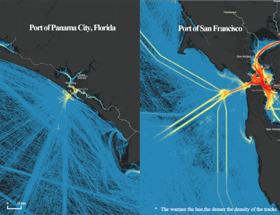
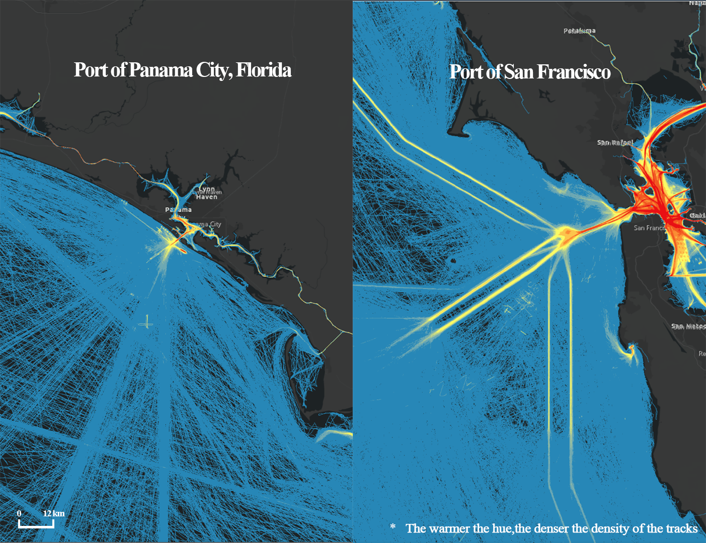
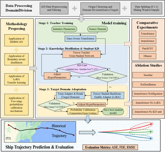
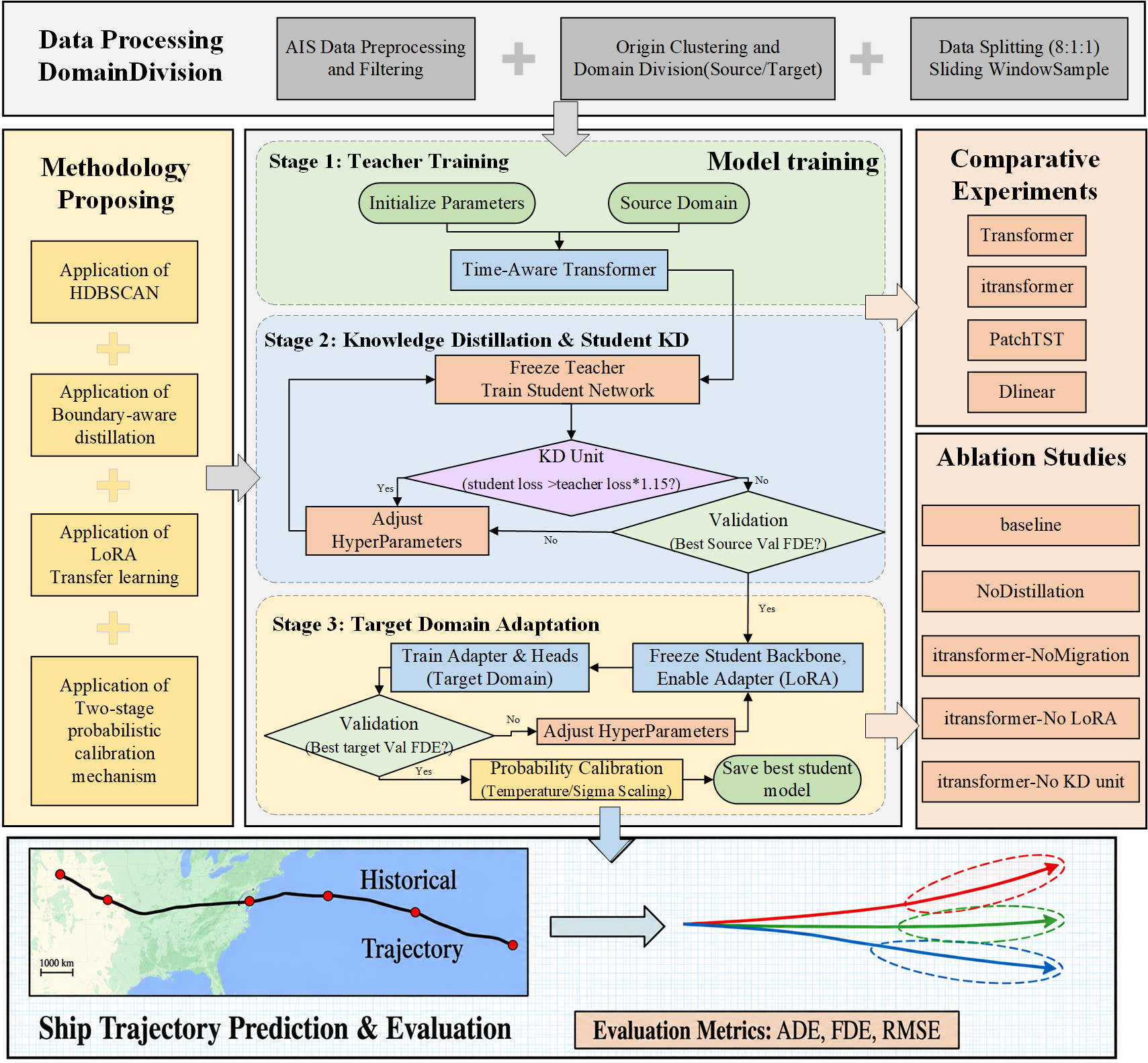
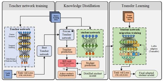
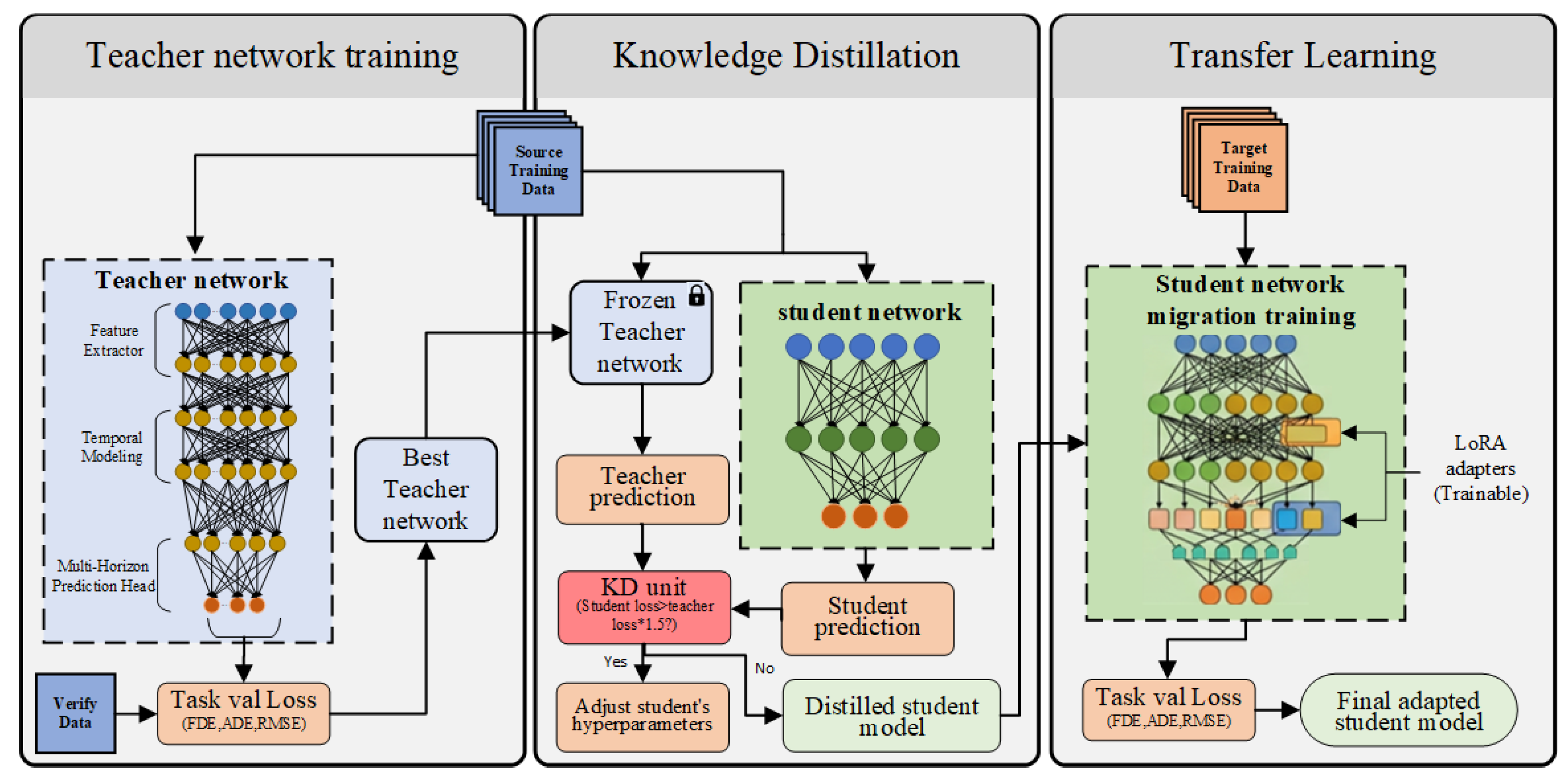
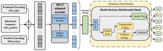
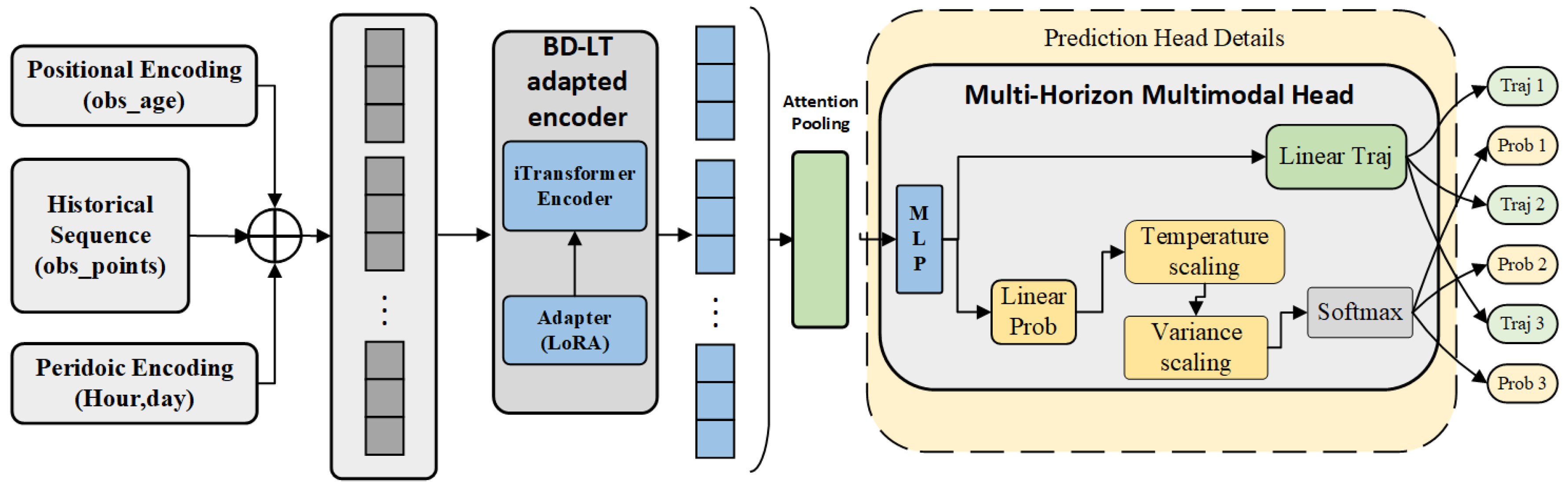
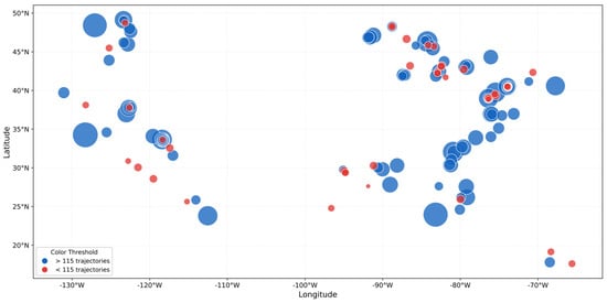
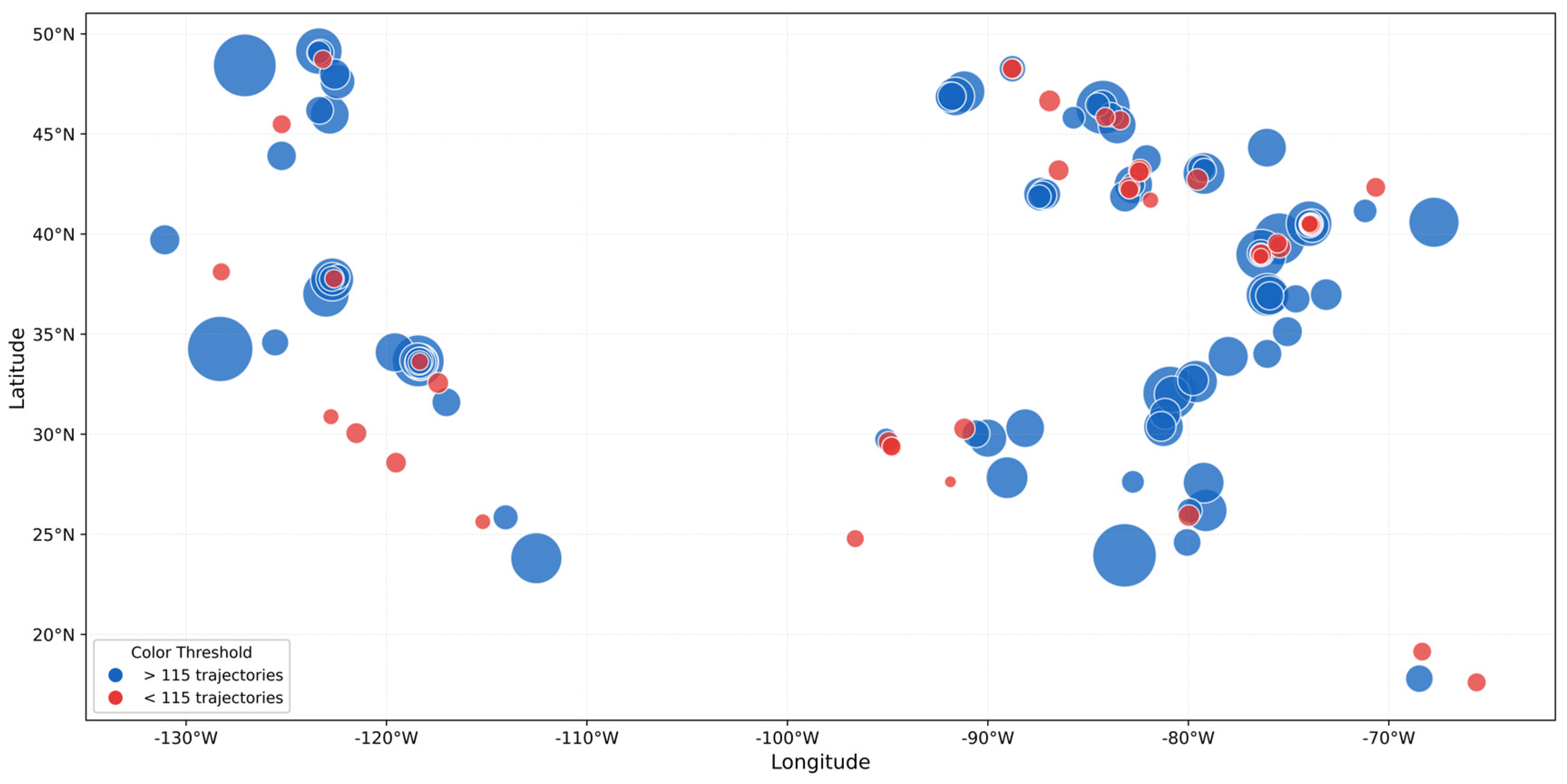
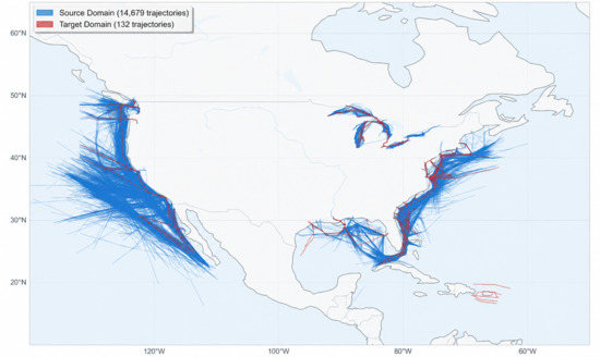
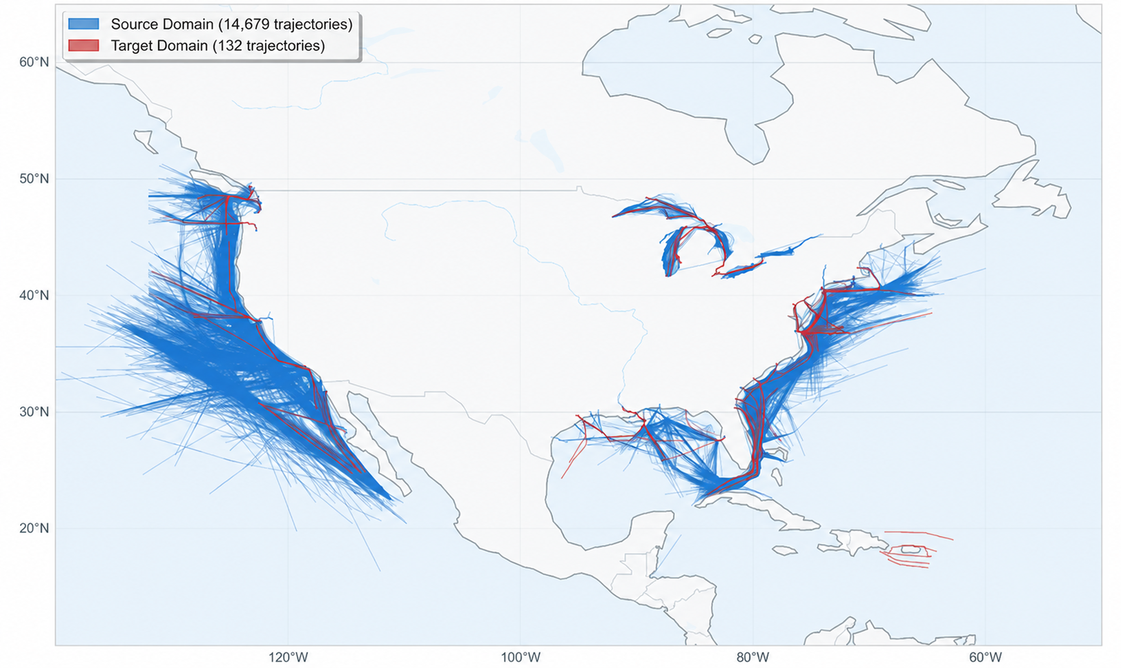
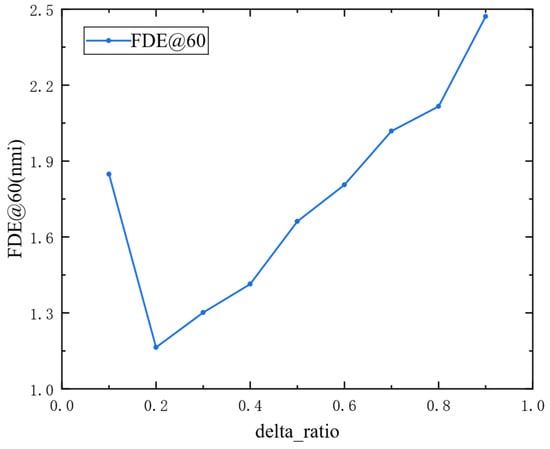
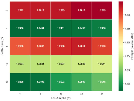
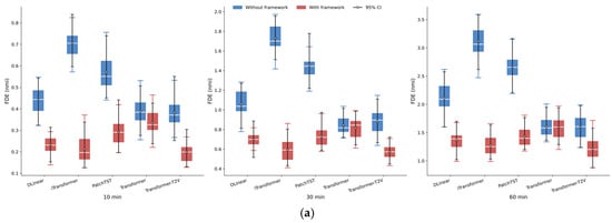
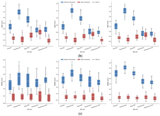
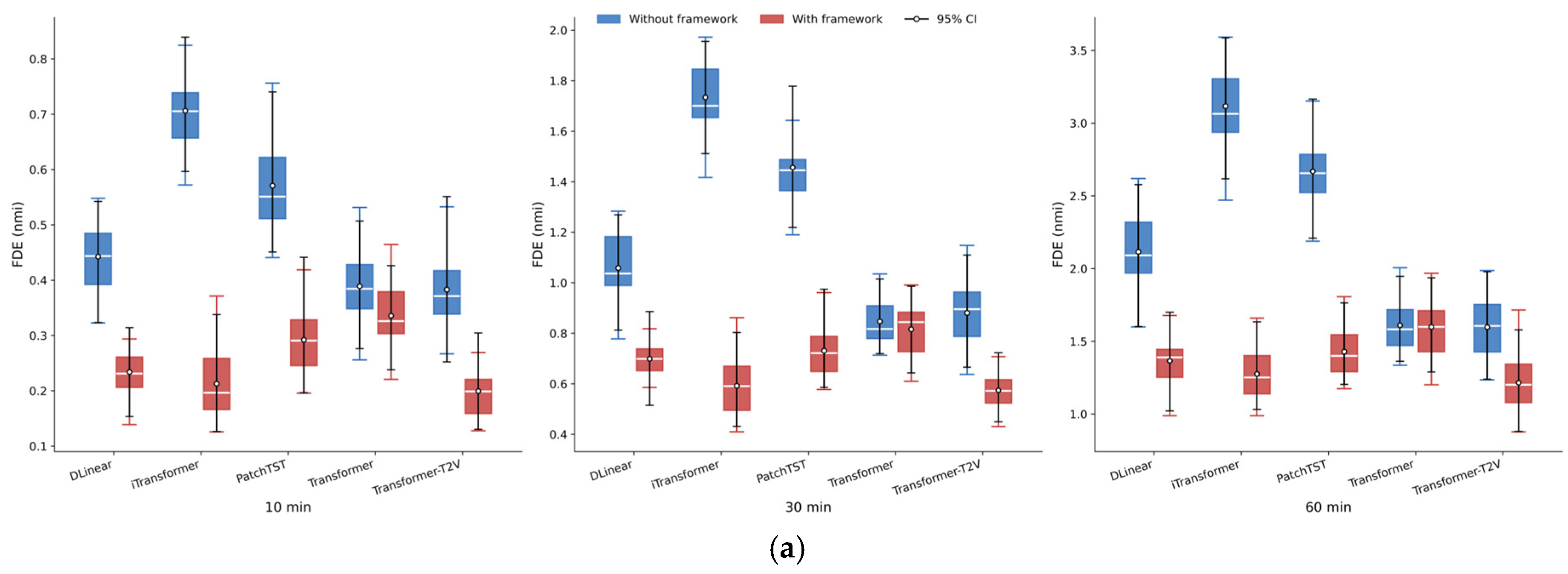
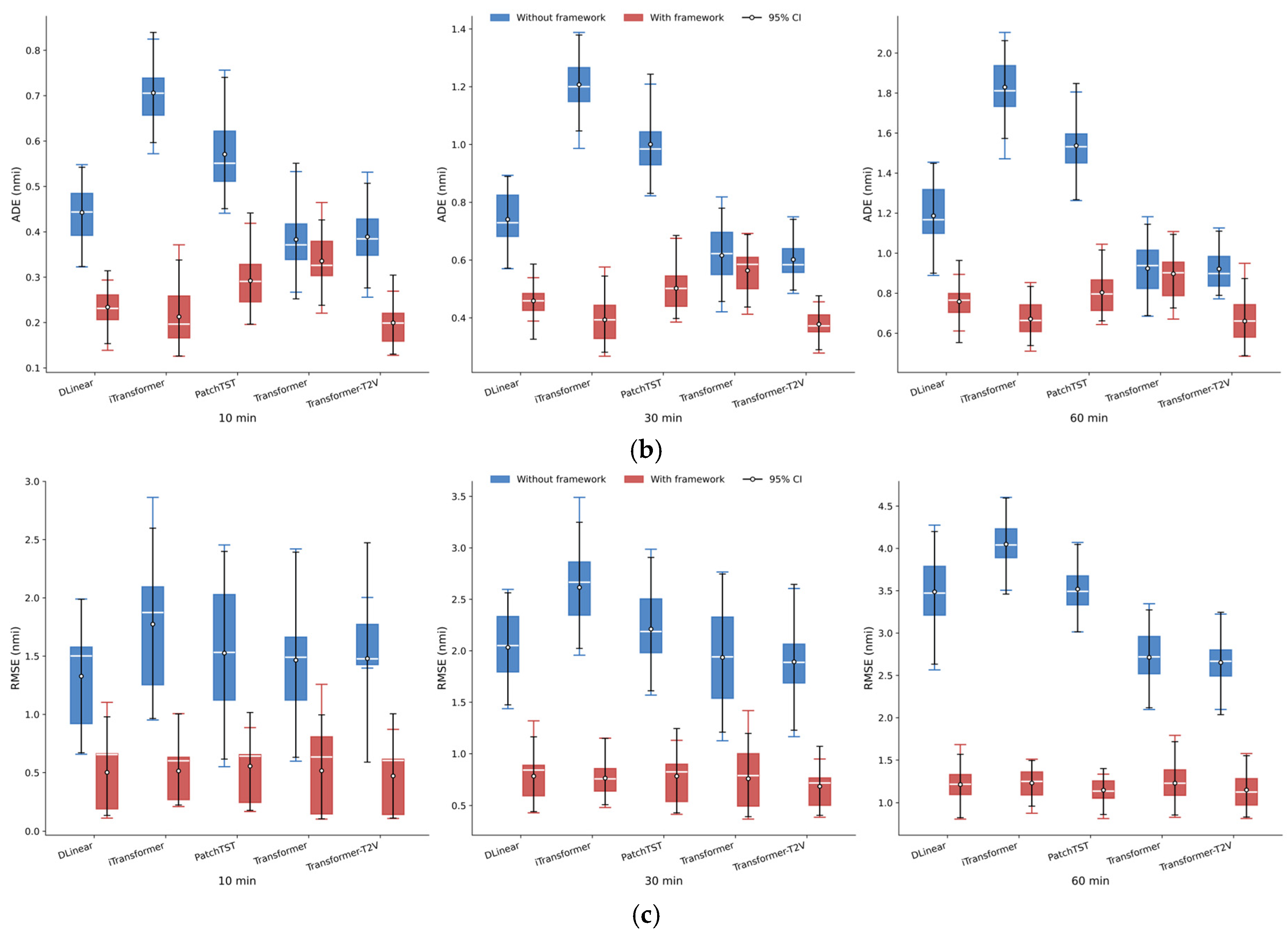
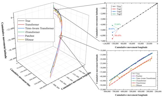
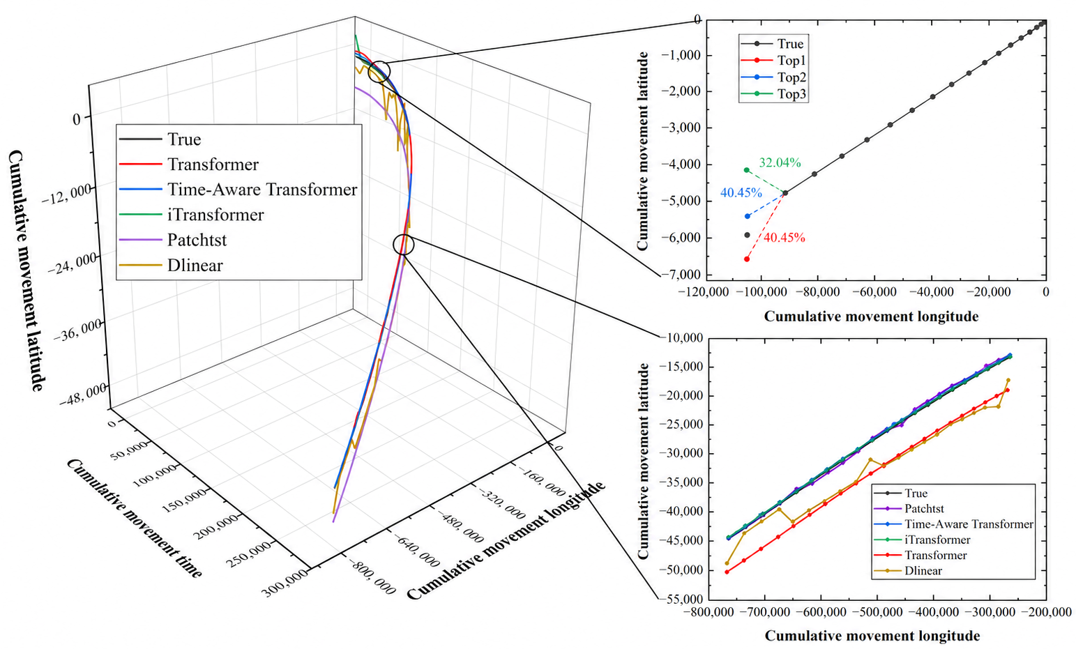
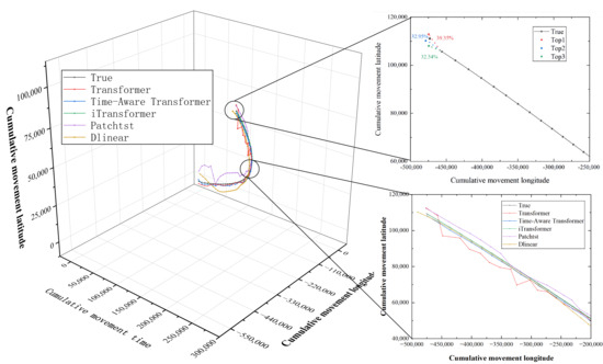
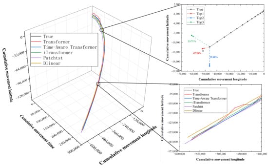
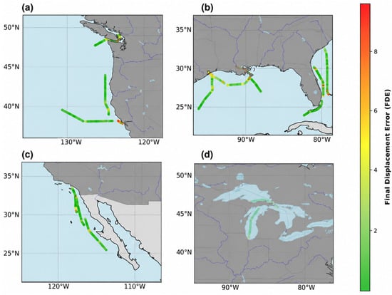
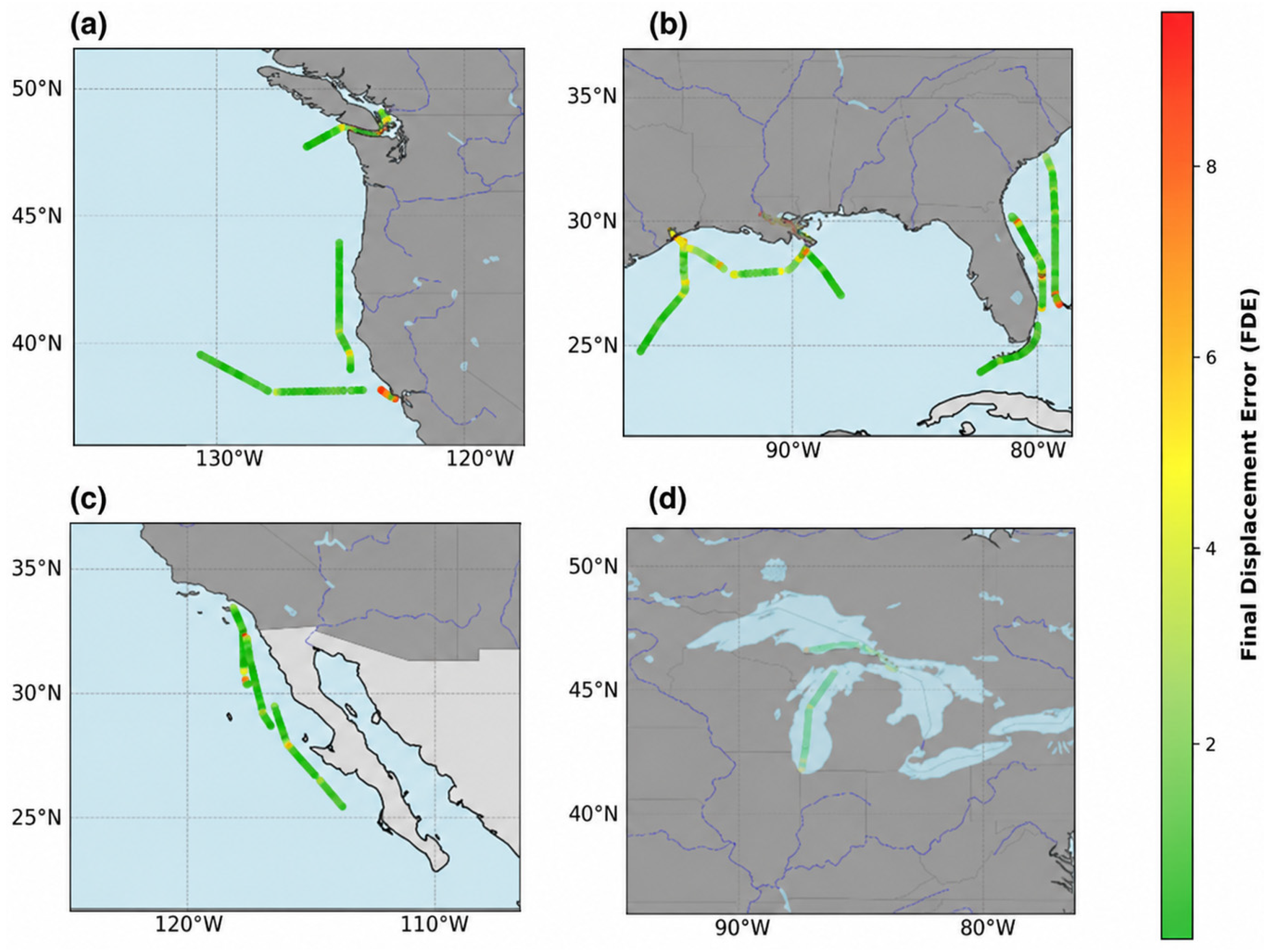
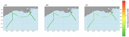
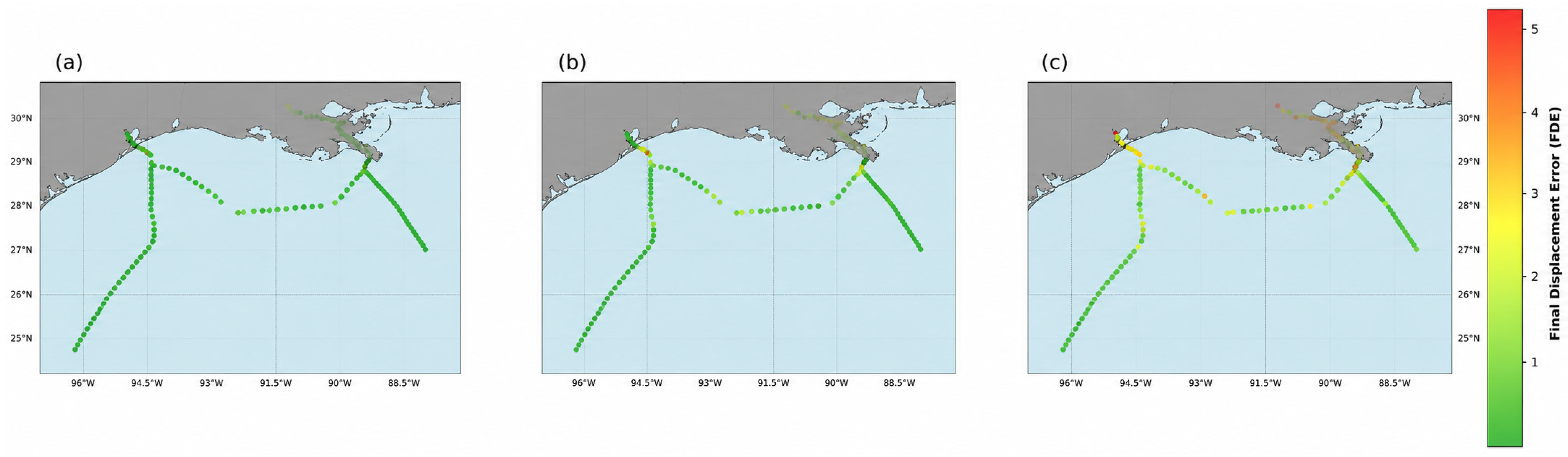

Disclaimer/Publisher’s Note: The statements, opinions and data contained in all publications are solely those of the individual author(s) and contributor(s) and not of MDPI and/or the editor(s). MDPI and/or the editor(s) disclaim responsibility for any injury to people or property resulting from any ideas, methods, instructions or products referred to in the content. |
© 2026 by the authors. Licensee MDPI, Basel, Switzerland. This article is an open access article distributed under the terms and conditions of the Creative Commons Attribution (CC BY) license.