Physical Prior Knowledge-Guided Reconstruction of Continuous Rice Canopy Spectra from UAV Multispectral Observations

Abstract

Unmanned aerial vehicle (UAV) multispectral imaging supports efficient crop monitoring but provides limited information on continuous spectral features. This study reconstructed rice canopy reflectance from 400 to 1000 nm using four UAV bands and evaluated whether the recovered spectra remained consistent across scales. Multispectral reflectance data acquired at three flight altitudes were used to analyze their consistency with canopy hyperspectral reflectance, and two data simulation methods coupled with PROSAIL-D were employed to compare the constraining effects of prior knowledge data. Cubic spline, piecewise linear–logistic (PLL), partial least squares regression (PLSR), multilayer perceptron (MLP), and SE-ResNet-Att models were compared across different validation sets. The results showed that a flight altitude of 50 m provided the closest agreement with ground canopy spectra (RMSE, 5.085%). Machine learning models showed higher accuracy based on the C-Vine method than the Monte Carlo sampling method, owing to the narrower spectral datasets generated by the joint parameters. With full-prior training, PLSR performed best with ground-resampled inputs (RMSE, 1.352%), whereas SE-ResNet-Att achieved the lowest UAV-field RMSE of 4.298%. However, the proposed model showed limited advantages over simpler models in the leave-one-growth-stage-out validation and model ablation experiment, indicating that the benefits of increasing network complexity were limited. Although reconstructed spectra reproduced broad red-edge and near-infrared patterns, blue relative errors and red-edge absolute errors remained prominent with UAV inputs. The reconstructed red-edge position was correlated with measured values (r = 0.928) but showed a negative bias (ranging from −20 to −9 nm). Its exploratory correlations with canopy water and nitrogen contents (r = 0.589 and 0.727) decreased to 0.110 and 0.203 after adjustment for growth stage and leaf area index relationships. The method proposed in this study supports the extraction and exploratory analysis of additional spectral features from UAV multispectral imagery, but quantitative trait estimation and transfer across independent fields, years, and rice cultivars require further validation.

1. Introduction

Canopy spectral reflectance provides a non-destructive description of crop biochemical and structural status because the absorption and scattering of incident radiation vary with leaf pigments, water and dry matter contents, mesophyll structure, leaf area index, leaf angle distribution, canopy closure, and background conditions [1]. Continuous spectra are particularly valuable because they preserve spectral shape, derivatives, and local absorption and scattering features that cannot be fully represented by broadband vegetation indices. The red-edge region is especially responsive to changes in pigment abundance and canopy development, and red-edge position (REP) has been used to characterize nitrogen-related variation in rice canopies [2]. Repeated spectral observations can therefore reduce reliance on destructive sampling and support spatially continuous crop monitoring, which has consequently become a central basis for rapid, non-destructive assessment of crop growth over large areas. However, field spectroradiometers cover limited areas, whereas unmanned aerial vehicle (UAV)-based hyperspectral systems remain constrained by sensor cost, payload, radiometric calibration, data volume, and processing requirements.

UAV equipped with multispectral sensors can acquire high spatial resolution broadband imagery, typically covering the blue, green, red, red-edge, and near-infrared regions. Owing to their non-contact data acquisition and operational flexibility, UAV multispectral systems have become important tools for field monitoring, including the retrieval of leaf area index, chlorophyll content, canopy water and nutrient status, and crop yield. However, each broadband measurement represents a spectral response function (SRF) weighted average and therefore does not directly preserve within-band spectral shape, derivative information, weak absorption features, or the precise red-edge position (REP). Their comparability with ground canopy spectra is also affected by illumination, radiometric calibration, viewing geometry, flight altitude, spatial resolution, and the proportions of vegetation, soil, water, and shadow within the sensor footprint. Previous studies have shown that flight altitude and calibration strategy can alter UAV-derived crop reflectance and the accuracy of downstream trait estimation [3,4]. Consequently, the operational multispectral input should first be evaluated against ground spectral observations at comparable spectral bands and spatial support.

Computational spectra reconstruction seeks to infer a dense and continuous spectrum from a limited set of broadband observations. Because the number of observed bands is much smaller than the number of target wavelengths, this inverse problem is non-unique and its solution depends strongly on the adopted spectral prior. Sparse dictionaries, adversarial networks, and residual or densely connected convolutional networks have demonstrated the feasibility of reconstructing hyperspectral images from RGB observations [5,6,7]. However, these approaches are generally trained on paired natural images and frequently exploit spatial texture, whereas crop applications require calibrated reflectance reconstruction under crop-specific biochemical, structural, and scale conditions. In vegetation studies, Togeiro de Alckmin et al. [8] reconstructed the 550–790 nm spectral shape of perennial ryegrass canopies using piecewise parametric functions, although fixed analytical forms may smooth local spectral variability. More recently, Wang et al. [9] coupled PROSAIL-PRO simulations with convolutional neural networks to reconstruct 400–2500 nm crop spectra from UAV multispectral observations and evaluated their use for nitrogen monitoring. These advances demonstrate the potential of physically informed spectral reconstruction, but the respective effects of prior construction, model complexity, and measurement-scale mismatch remain insufficiently separated.

Radiative transfer models provide a mechanism for constructing crop spectral priors by linking leaf biochemical properties, canopy architecture, soil background, and observation geometry to physically plausible reflectance [10]. PROSAIL-based simulations have consequently been used to support spectra sampling, crop-trait retrieval, and machine learning model training [11,12]. Nevertheless, assigning physically reasonable ranges to individual parameters does not ensure that their combinations represent coordinated crop growth states. Independent parameter sampling may neglect empirical dependencies among chlorophyll, water content, dry matter, leaf area, and canopy structure, thereby increasing the difference between simulated and measured spectra [13]. Crop-specific Bayesian inversion and phenological archetype models have demonstrated the value of joint parameter distributions and coordinated crop-trait dynamics for constraining PROSAIL simulations [14,15]. C-vine copulas offer a flexible way to represent such multivariate dependencies through conditional pair-copula decompositions [16]. They can therefore be used to construct a crop-informed spectral prior while retaining the marginal distributions of individual growth parameters. However, the influence of a C-vine joint prior on four-band spectral reconstruction, and whether increasingly complex networks can exploit this information more effectively than simpler models, have not been systematically evaluated.

To address these issues, this study evaluated a physically guided framework for reconstructing continuous rice canopy reflectance over 400–1000 nm from four UAV multispectral bands: green, red, red-edge and near-infrared. Spectral consistency between leaves and canopies was first evaluated. UAV reflectance acquired at 20, 50, and 100 m was then compared with canopy observations to identify a suitable flight altitude for this study. The independent Monte Carlo (MC) method was compared with a crop-constrained C-Vine method to assess how prior construction using PROSAIL-D affected spectra reconstruction accuracy. Furthermore, the reconstructed REP was evaluated through its agreement with measured REP and its exploratory associations with canopy water content and canopy nitrogen content. The study therefore addressed three questions: (1) which tested flight altitude provided the closest agreement with ground canopy observations; (2) how joint parameter priors and model complexity affected reconstruction performance across validation scales; and (3) whether the reconstructed REP could establish reliable relationships with rice water and nitrogen status.

2. Materials and Methods

2.1. Study Area and Experiments

The experiment was conducted in 2023 at the Changshu Water Conservancy Technology Extension Station in Xinzhuang Town, Changshu City (31°32′47.07″ N, 120°42′4.27″ E). The rice cultivar Changxiangjing 1813 was transplanted on 21 June at a spacing of 25 cm × 15 cm and harvested on 25 October. Two irrigation treatments, shallow frequent irrigation (W1, with lower and upper irrigation limits of 10 and 30 mm, respectively) and controlled irrigation (W2, with lower and upper irrigation limits of 80% and 100% of saturated water content, respectively), were combined with 75 (N1), 255 (N2), and 375 (N3) kg/hm² pure nitrogen application rates. Due to site area constraints, the low- and high-nitrogen treatments (N1 and N3) were replicated twice, while the standard nitrogen treatment (N2) had no replicates, resulting in a total of 10 experimental plots. Phosphorus and potassium fertilizers were applied once as basal fertilizer in each plot at rates of 75 kg/hm² (P₂O₅) and 105 kg/hm² (K₂O), respectively. Pure nitrogen was applied in proportions of 35%, 35%, and 30% at the pre-transplanting, tillering, and panicle stages, respectively.

2.2. Data Collection

2.2.1. Spectral Reflectance Measurements

Leaf and canopy hyperspectral reflectance (400–2500 nm) were measured using a PSR+3500 portable field spectroradiometer (Spectral Evolution, Lawrence, MA, USA) operated with DARWin SP (V1.3, Spectral Evolution, Lawrence, MA, USA) software. On the same day as the UAV flight, the canopy probe was directed vertically downward, approximately 30 cm above the canopy with a field of view of 25° around 11:00 under natural sunlight. A standard white reference panel (reflectance >99%) was measured before and after each measurement to minimize noise caused by fluctuations in sunlight. Measurements were conducted at five points in each plot and ten scans were averaged for each measurement. The five resulting spectra were then averaged to obtain the plot-level spectra reflectance. Savitzky–Golay (S–G) smoothing was subsequently applied to the spectra and the smoothed spectra were used as the measured references for accuracy evaluation.

Canopy multispectral imagery was acquired using a MAVIC 3M multispectral drone (Shenzhen Dajiang Innovation Technology Co., Ltd., Shenzhen, China), which records reflectance in green (G, 560 ± 16 nm), red (R, 650 ± 16 nm), red-edge (RE, 730 ± 16 nm), and near-infrared (NIR, 860 ± 26 nm) bands with an effective resolution of 5 megapixels. Multispectral imagery was acquired around 11:00 AM during clear or partly cloudy weather at tillering, jointing–booting, heading–flowering and milking stages. Three flight altitudes (20 m, 50 m, and 100 m) were set, with 85% forward overlap and 85% side overlap. Specific flight parameters for each mission are listed in Table 1.

Table 1. Detailed parameters for each flight.

Flight Date	Time	Solar Elevation (°)	Altitude (m)	Number of Images	Resolution (mm/Pixel)
31 July	11:00 a.m.	70.45	20/50/100	576/204/56	10/20/50
24 August	11:00 a.m.	65.38	20/50/100	576/204/56	10/20/50
1 September	11:00 a.m.	63.33	20/50/100	576/204/56	10/20/50
17 September	11:00 a.m.	58.34	20/50/100	576/204/56	10/20/50

Before each flight, images of a standard white reference panel (reflectance >99%) were acquired for radiometric calibration. In addition, the integrated spectral sunlight sensor of the Mavic 3M also continuously recorded incident solar irradiance during each flight. The multispectral images were processed using PIE-SMART (Version 6.0; Beijing Piesat Information Technology Co., Ltd., Beijing, China), where image alignment, mosaicking, and radiometric correction were performed using the reference panel measurements. The calibrated images were subsequently exported as georeferenced TIFF orthomosaics. Plot-level reflectance was extracted from the multispectral orthomosaics using manually delineated regions of interest (ROIs) following the boundaries of each 9 m × 9 m experimental plot. The normalized difference vegetation index (NDVI) was calculated within each ROI, and exposed water and bare soil were excluded by manually selecting NDVI thresholds (with NDVI of 0.33, 0.45, 0.45 and 0.37 for tillering, jointing–booting, heading–flowering and milking stages, respectively). The resulting vegetation mask was applied to all four multispectral bands. Plot-level reflectance was then calculated as the mean of all retained vegetation pixels within each ROI for each band.

2.2.2. Rice Physiological and Biochemical Parameters

Rice samples were collected concurrently with the acquisition of spectral reflectance data to construct a prior dataset for spectral reflectance simulation. Five 1 m × 1 m quadrats were selected within each plot of N1 and N3 and ten quadrats were selected within each N2 plot. Leaf area index (LAI) was measured using a SunScan canopy analysis system (Delta-T Devices Ltd., Cambridge, UK). Chlorophyll a + b contents (Cab) and carotenoid contents (Car) were determined by spectrophotometry (Shanghai Jingke Scientific Instrument Co., Ltd., Shanghai, China). Leaf water content (LWC) and leaf dry matter mass (LDM) were obtained using the oven-drying method. Average leaf inclination angle (ALA) was determined using the MultispeQ (PHOTOSYNQ INC., East Lansing, MI, USA). Leaf total nitrogen content (LNC) was determined using the Kjeldahl nitrogen analyzer (Shanghai Lichen Instrument Technology Co.,Ltd, Shanghai, China). Canopy water content (CWC) and canopy nitrogen content (CNC) were calculated by multiplying the treatment-stage mean LWC or LNC by the corresponding LAI. Ten sampling records were obtained per treatment at each growth stage. For N1 and N3 treatments, five records came from each of the two replicate plots, while all ten records for the N2 treatment came from its single plot.

2.2.3. Red-Edge Position Extraction

Red-edge position (REP) was defined as the wavelength of the maximum first derivative of canopy reflectance within 700–760 nm. Measured and reconstructed spectra received the same smoothing strategy. The first derivative was calculated by central differences on the 1 nm grid. Tied maxima were resolved by choosing the shorter wavelength.

2.3. Radiative Transfer Model and Data Simulation Method

The PROSAIL-D model was used to simulate canopy spectral reflectance. It couples the leaf optical properties model PROSPECT-D and the canopy radiative transfer model 4SAIL. Empirical ranges for the rice input parameters were listed in Table 2 [17,18,19].

Table 2. Empiric value ranges of PROSAIL-D model input parameters.

Parameters	Abbreviations	Range	Unit
Leaf structure parameter	Ns	[1.3, 2.5]	-
Chlorophyll a + b content	Cab	[0, 80]	μg/cm2
Carotenoid content	Car	[0, 20]	μg/cm2
Anthocyanin content	Canth	[0, 15]	μg/cm2
Brown pigments content	Cbrown	[0, 1]
Equivalent water thickness	Cw	[0.001, 0.100]	cm
Dry matter content	Cm	[0.001, 0.060]	g/cm2
Average leaf inclination angle	ALA	[0, 90]	°
Leaf area index	LAI	[0, 8]	-
Hotspot parameter	hotspot	0.5/LAI	-
Dry/wet soil factor	psoil	[0, 1]	-
Leaf angle distribution type	TypeLIDF	2	-
Solar zenith angle	tts	20	°
Observe zenith angle	tto	0	°
Relative azimuth angle	psi	0	°

Two data generation methods were employed in this study. For the MC method, 10,000 independent parameter combinations were generated using Simlab according to the empirical input parameter ranges listed in Table 2. For the C-Vine method, the joint distributions of measured growth parameters, including Cab, Car, Cw, Cm, LAI and ALA, were fitted separately for the tillering, jointing–booting, heading–flowering and milking stages, using 60 physiological sampling records per stage. Each stage-specific prior generated 2500 parameter combinations through random sampling, giving a combined dataset of 10,000 in total. The C-Vine copula was constructed in R using the VineCopula package (v2.6.1). Detailed methodological procedures could be found in our previous study [20].

The parameter combinations from different generation methods were then used as inputs to the PROSAIL-D model to generate the corresponding spectral reflectance dataset. The effects of anthocyanins (Canth) and brown pigments (Cbrown) were not considered in the current simulation and both were set to zero. As the spectra measurements were conducted before noon, fixed values of 20°, 0°, and 0° were adopted for tts, tto, and psi, respectively. For p_soil, 25% of the values were set to 0, 25% were set to 1, and the remaining 50% followed a normal distribution within the 0–1 range. Ns was calculated using the formula proposed by Jacquemoud and Baret [21]. Cw and Cm were calculated based on LWC and LDM [22].

$$\mathit{Ns}={\displaystyle \frac{0.9\mathit{LSA}+0.025}{\mathit{LSA}-0.1}}$$

(1)

$$\mathit{Cm}={\displaystyle \frac{\mathit{LDM}}{A}}$$

(2)

$$\mathit{Cw}={\displaystyle \frac{\mathit{LFM}-\mathit{LDM}}{A}}$$

(3)

where LSA is leaf specific area, cm²/mg. In this study, LSA = 1/(1000 Cm). Cm is the dry matter content, g/cm². Cw is the equivalent water thickness, cm. LDM and LFM are the dry and fresh mass weight of leaf samples, respectively. A represents the area of the leaf samples.

2.4. Models for Spectra Reconstruction

This study evaluates the accuracy of five models in reconstructing continuous spectra (400–1000 nm) based on four-band reflectance data. These models include the cubic spline model, piecewise linear–logistic fitting model (PLL), partial least squares regression model (PLSR), multilayer perceptron model (MLP), and squeeze-and-excitation residual attention neural network model (SE-ResNet-Att).

Specifically, the cubic spline model performs interpolation using the four multispectral central wavebands as nodes and extrapolates the data to 1000 nm. The PLL model is based on the method proposed by Togeiro de Alckmin [8]: linear interpolation is used for the 400–685 nm range, defined by the G and R central wavebands; for the 685–1000 nm range, a three-parameter logistic curve is used, which starts at the R band, approaches the NIR band asymptotically with a growth rate determined by the RE band, followed by extrapolation to 1000 nm.

The PLSR model was implemented using the NIPALS algorithm. The number of latent variables was selected from 1 to 4 by minimizing RMSE on the simulated validation subset, and the final number of latent variables was set to 4. The MLP model only comprised one single hidden layer with 32 units and ReLU activation with a learning rate of 0.0012.

The proposed SE-ResNet-Att model applied a learned 4 × 4 input attention transformation (with gates scaled as twice the sigmoid outputs) to the four-band inputs. The gated inputs were projected to 64 hidden units and passed through one residual block with a residual scale of 0.5. An SE block with a 64–8–64 bottleneck and twice-sigmoid gates recalibrated the hidden features before decoding them to 601 wavelengths. ResNet omitted both the SE and input attention modules, while SE-ResNet omitted input attention. MLP, SE-ResNet-Att and corresponding ablation models were trained using full-batch Adam with a learning rate of 0.0012, weight decay of 10⁻⁵ and a maximum of 260 training epochs.

The gate inputs were projected to 64 hidden units and passed through one 64-unit residual block with a residual scale of 0.5 and a learning rate of 0.0012; then an SE block with a 64-to-8-to-64 bottleneck (with gates scaled as twice the sigmoid outputs) was applied and decoded to 601 wavelengths between 400 and 1000 nm.

For MLP, SE-ResNet-Att models and their corresponding ablation models, a composite loss function was constructed by jointly considering weighted reflectance error, first-derivative spectral error, and SRF consistency error. This formulation was designed to improve the reconstruction accuracy of canopy reflectance over 400–1000 nm under the dual constraints of local spectral-shape continuity and consistency with multispectral sensor observations. The weighted mean squared error penalized reflectance errors across the full spectrum. The first-derivative loss constrained wavelength-to-wavelength variations, whereas the SRF consistency loss required the reconstructed spectrum to reproduce the observed G, R, RE, and NIR inputs.

L_total = L_MSE + α_derL_der + α_SRFL_SRF

(4)

$$L_{\mathit{MSE}}={\displaystyle \frac{1}{N{\displaystyle {\sum }_{\lambda =1}^L{\omega }_{\lambda }}}}{\displaystyle \sum _{i=1}^N{\displaystyle \sum _{\lambda =1}^L{\omega }_{\lambda }{\left(y_{i,\lambda }-x_{i,\lambda }\right)}^2}}$$

(5)

$$L_{\mathit{der}}={\displaystyle \frac{1}{N\left(L-1\right)}}{\displaystyle \sum _{i=1}^N{\displaystyle \sum _{\lambda =1}^{L-1}{\left[\left(y_{i,\lambda +1}-y_{i,\lambda }\right)-\left(x_{i,\lambda +1}-x_{i,\lambda }\right)\right]}^2}}$$

(6)

$$L_{\mathit{SRF}}={\displaystyle \frac{1}{4N}}{\displaystyle \sum _{i=1}^N{\displaystyle \sum _{b=1}^4{\left({\displaystyle \sum _{\lambda =1}^L\mathit{SR}{F}_{\lambda ,b}}{y}_{i,\lambda }-x_{i,b}^{\mathit{MS}}\right)}^2}}$$

(7)

where L_total, L_MSE, L_der, L_SRF are the total loss function, mean squared error loss function, first-derivative loss function and SRF loss function, respectively. α_der and α_SRF are the weights of L_der and L_SRF, respectively. After multiple tests to balance the constraints of the two loss functions on the overall reconstruction accuracy, the values were set to 0.02 and 0.10, respectively. The weight ω_λ was set to 1.5 over the 680–760 nm range and to 1 in elsewhere to emphasize the red-edge reconstruction. x_i,λ and y_i,λ are number λ wavelength of the target and reconstructed spectral reflectance, respectively. N is the number of the samples. L is the number of the wavelengths between 400 and 1000 nm. b is the number of the multispectral bands, ranking by G, R, RE and NIR. SRF_λ,b is the SRF coefficient of number λ wavelength responding to multispectral band b. x_i,b^MS is the target multispectral reflectance of band b.

The network architectures and optimization settings were chosen empirically during preliminary experiments using the training and validation subsets of the simulated spectra datasets. The derivative and SRF loss weights were adjusted using those subsets to balance reflectance reconstruction with derivative and SRF consistency. These settings were then held fixed for the final evaluations. Neither the simulated test subset nor the 24 measured canopy spectra were used for model or hyperparameter selection.

2.5. Dataset Splitting and Processing

To construct the input–output pairs for spectra reconstruction, the canopy spectral reflectance generated by PROSAIL-D was resampled using the SRFs of the Mavic 3M multispectral sensor (measured by Optics of Photosynthesis Lab, University of Helsinki). For each simulated canopy spectrum, the reflectance of the four multispectral bands, G, R, RE, and NIR, was calculated by integrating the narrow-band reflectance weighted by the corresponding SRF. This process produced a simulated reconstruction dataset in which the four-band multispectral reflectance was used as the model input, and the 400–1000 nm narrow-band canopy reflectance was used as the reconstruction target.

The reconstruction accuracy of the models was first evaluated using 10-fold cross-validation on each 10,000 simulated spectra generated by different methods. Random seed 42 was used to assign samples to ten equal folds, in which each iteration used 90% for training and 10% for testing. The results were characterized by the average accuracy and the standard deviation of the accuracy obtained from the 10-fold cross-validation.

To further evaluate model performance on measured data, the same Mavic 3M SRFs were applied to the 24 measured treatment-level canopy hyperspectral reflectance spectra, which were the mean values of each water–nitrogen treatment at each of the four stages. The resampled reflectance values were used as ground inputs for field-scale validation, while the four-band reflectance values extracted from the UAV imagery were averaged by treatment for UAV-field-scale validation. For the full-prior evaluation, the simulated spectra based on C-Vine method were divided into training (80%), validation (10%) and test (10%) subsets with random seed 42. All machine learning models were trained on the same training subset and tuned using the same validation subset. The same trained models were used for both field-scale and UAV-field-scale validations, with all 24 measured hyperspectral spectra used as target spectra.

In particular, a leave-one-growth-stage-out validation was further performed for the C-vine-based simulation dataset. In each fold, the 2500 simulated spectra corresponding to one growth stage were excluded. The remaining 7500 spectra were split into training (80%), validation (10%) and test (10%) subsets with random seed 42, using the same fitting and validation-based selection procedures as in the full-prior evaluation. The reconstruction methods were then evaluated on the six treatment-level observations from the excluded stage, using ground SRF-resampled multispectral reflectance and UAV multispectral reflectance as two separate input sources, with the corresponding measured canopy hyperspectral spectra serving as references. This procedure was repeated for all four growth stages to evaluate the transferability of the reconstruction models across growth stages within the experiment when physiological information from the target stage were excluded from the C-Vine prior.

After model prediction, the reconstructed reflectance curves were smoothed using a Savitzky–Golay (S–G) filter (with a 21-point window, second-order polynomial, 1 nm spectral spacing) [23] to reduce local jagged fluctuations and spectral oscillations in the model outputs. All evaluation metrics were calculated using the smoothed reconstructed spectra and the corresponding reference spectra. The same S–G output-processing procedure was applied to all reconstruction methods. The measured reference spectra were also smoothed by the S–G filter (same parameters setting as for the reconstructed spectra) after export from DARWin SP software and were not smoothed again during metric calculation.

2.6. Evaluation Metrics

Root mean squared error (RMSE), relative root mean squared error (RRMSE), squared Pearson correlation (R²corr), Lin’s concordance correlation coefficient [24] (CCC), and spectral angle mapper (SAM) were employed to quantify the agreement between different spectra. For each pair of target reference and reconstructed spectra, these evaluation metrics were calculated separately and then averaged with equal weight.

$$\mathit{RMSE}=\sqrt{{\displaystyle \frac{1}{n}}{\displaystyle \sum _{i=1}^n{\left(y_i-x_i\right)}^2}}$$

(8)

$$\mathit{RRMSE}={\displaystyle \frac{\sqrt{\frac{1}{n}{\displaystyle \sum _{i=1}^n{\left(y_i-x_i\right)}^2}}}{\overline{x}}}$$

(9)

$$R_{\mathit{corr}}^2={\left[{\displaystyle \frac{{\displaystyle {\sum }_{i=1}^n\left(x_i-\overline{x}\right)\left(y_i-\overline{y}\right)}}{\sqrt{{\displaystyle {\sum }_{i=1}^n{\left(x_i-\overline{x}\right)}^2}}\sqrt{{\displaystyle {\sum }_{i=1}^n{\left(y_i-\overline{y}\right)}^2}}}}\right]}^2$$

(10)

$$\mathit{CCC}={\displaystyle \frac{2\rho {\sigma }_x{\sigma }_y}{{\sigma }_x^2+{\sigma }_y^2+{\left(\overline{x}-\overline{y}\right)}^2}}$$

(11)

$$\mathit{SAM}=\arccos \left({\displaystyle \frac{{\displaystyle {\sum }_{i=1}^n{x}_i{y}_i}}{\sqrt{{\displaystyle {\sum }_{i=1}^n{x}_i^2}}\sqrt{{\displaystyle {\sum }_{i=1}^n{y}_i^2}}}}\right)$$

(12)

where x_i and y_i are target and reconstructed spectral reflectance, respectively. $\overline{x} \mathrm{and} \overline{y}$ are the mean values of the target and reconstructed spectral reflectance, respectively. n is the number of the bands. ρ is the Pearson correlation coefficient. σ_x and σ_y are the standard deviation values of the target and reconstructed spectral reflectance, respectively.

The four multispectral inputs contained no blue band and only one NIR band at 860 nm. To assess reconstruction accuracy in regions with different spectral coverage, field-scale and UAV-field-scale errors were evaluated separately over 400–520, 521–679, 680–760, 761–879 and 880–1000 nm. Within each interval, RMSE was calculated for each spectrum and averaged across the 24 treatment-stage spectra, then RRMSE was calculated as this mean RMSE divided by the mean reference reflectance across all spectra and wavelengths in the same interval.

3. Results

3.1. Hyperspectral Characteristics and Consistency of Rice Leaves and Canopy

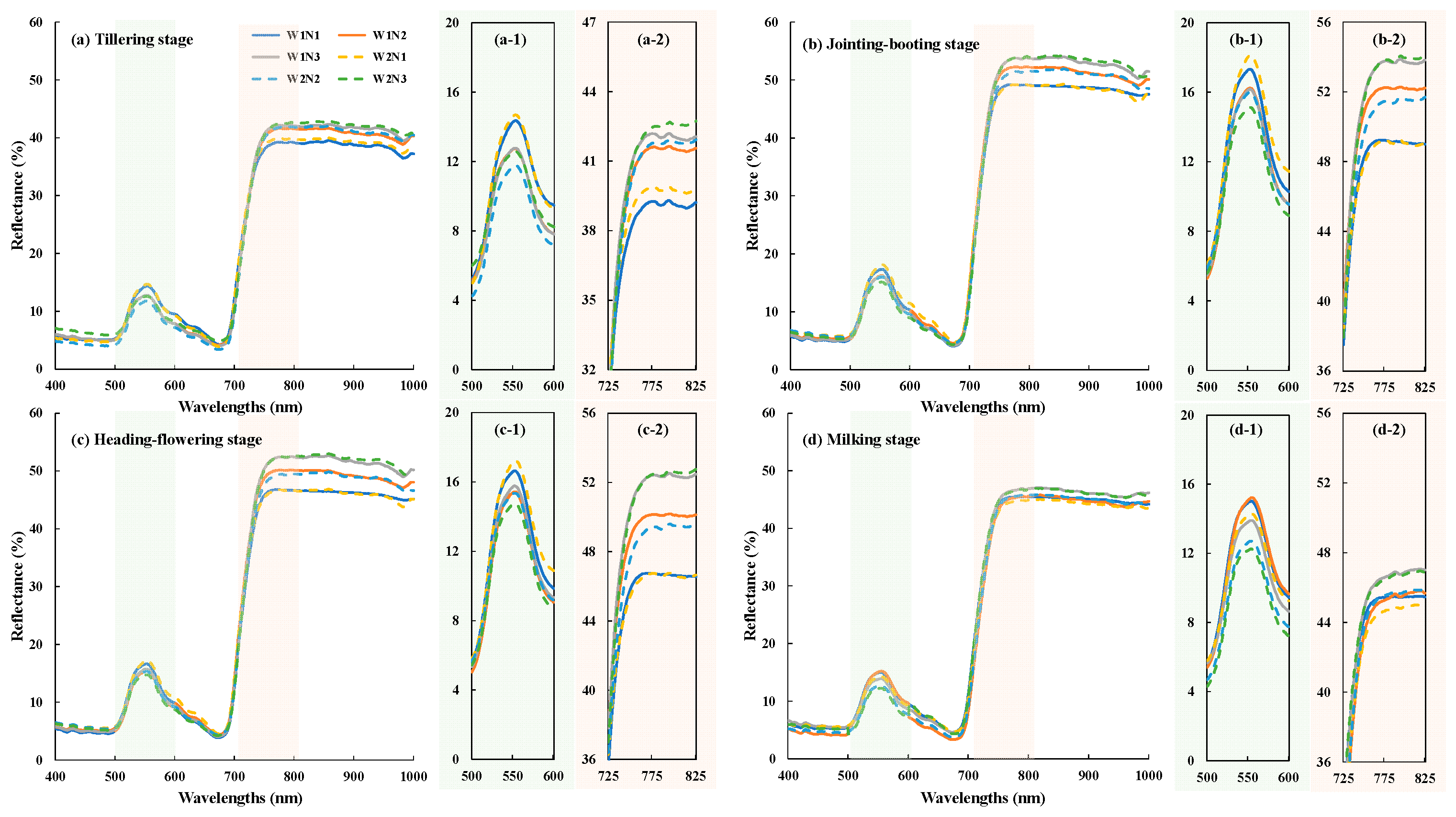
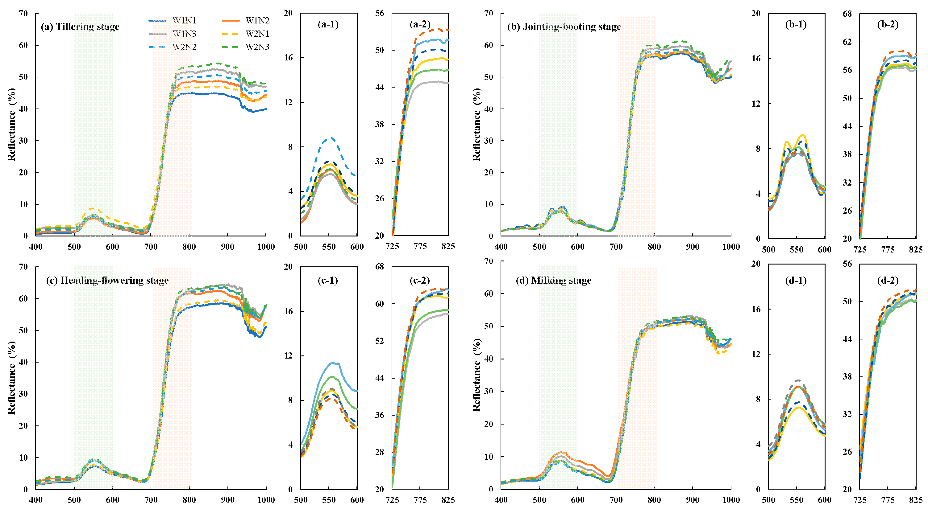
As shown in Figure 1 and Figure 2, leaf and canopy spectra exhibited similar expected vegetation patterns over 400–1000 nm: low visible reflectance with a green peak, strong chlorophyll absorption near the red region, a rapid red-edge rise, and a high near-infrared plateau. Compared with leaf spectra, canopy spectra showed a more pronounced water absorption feature at 970 nm. Additionally, irrigation regimes and nitrogen application levels had a more significant effect on canopy reflectance. W1 treatment with a standing water layer exhibited lower canopy reflectance due to water absorption during the early growth stage. While, higher nitrogen application rates promoted canopy expansion, thereby increasing reflectance in the near-infrared band while decreasing it in the green band.

Figure 1. Spectral reflectance curve of rice leaves at different growth stages. (a–d) are leaf spectral reflectance curve at the tillering, jointing–booting, heading–flowering and milking stages, respectively.

Figure 2. Spectral reflectance curve of rice canopies at different growth stages. (a–d) are canopy spectral reflectance curve at the tillering, jointing–booting, heading–flowering and milking stages, respectively.

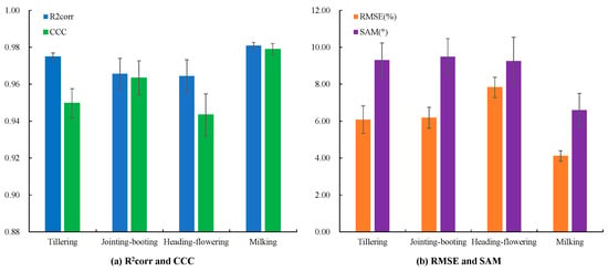
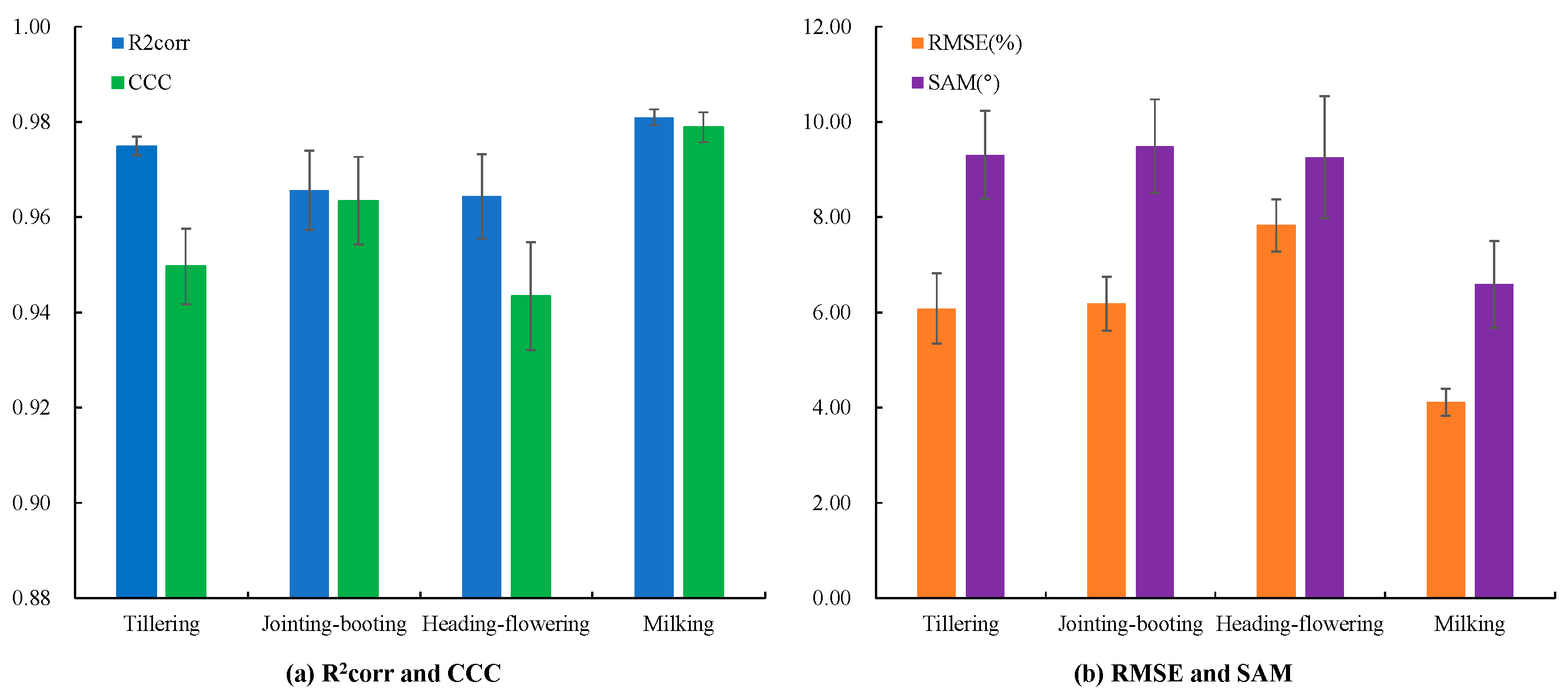
Figure 3 shows that the leaf and canopy spectral shapes were strongly correlated in the range of 400 nm to1000 nm at every growth stage, with mean R²corr values of 0.964–0.981 and CCC values of 0.943–0.979. Nevertheless, absolute and angular differences remained substantial: stage-mean RMSE ranged from 4.116% at the milking stage to 7.831% at the heading–flowering stage, while SAM ranged from 6.590° to 9.490°. The coexistence of high correlation and non-negligible RMSE indicated that leaf and canopy measurements shared the same broad spectral patterns but differed in value, because canopy reflectance additionally affected by the canopy structure and background.

Figure 3. The reflectance consistency between leaf and canopy across different stages. (a) shows the comparison of R²corr and CCC across growth stages. (b) shows the comparison of RMSE and SAM across growth stages.

3.2. Multispectral Characteristics at Different Flight Heights and Their Consistency with Ground Hyperspectral Data

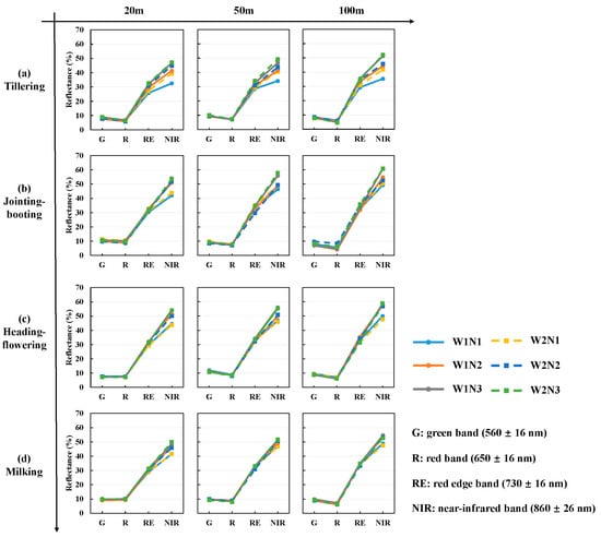
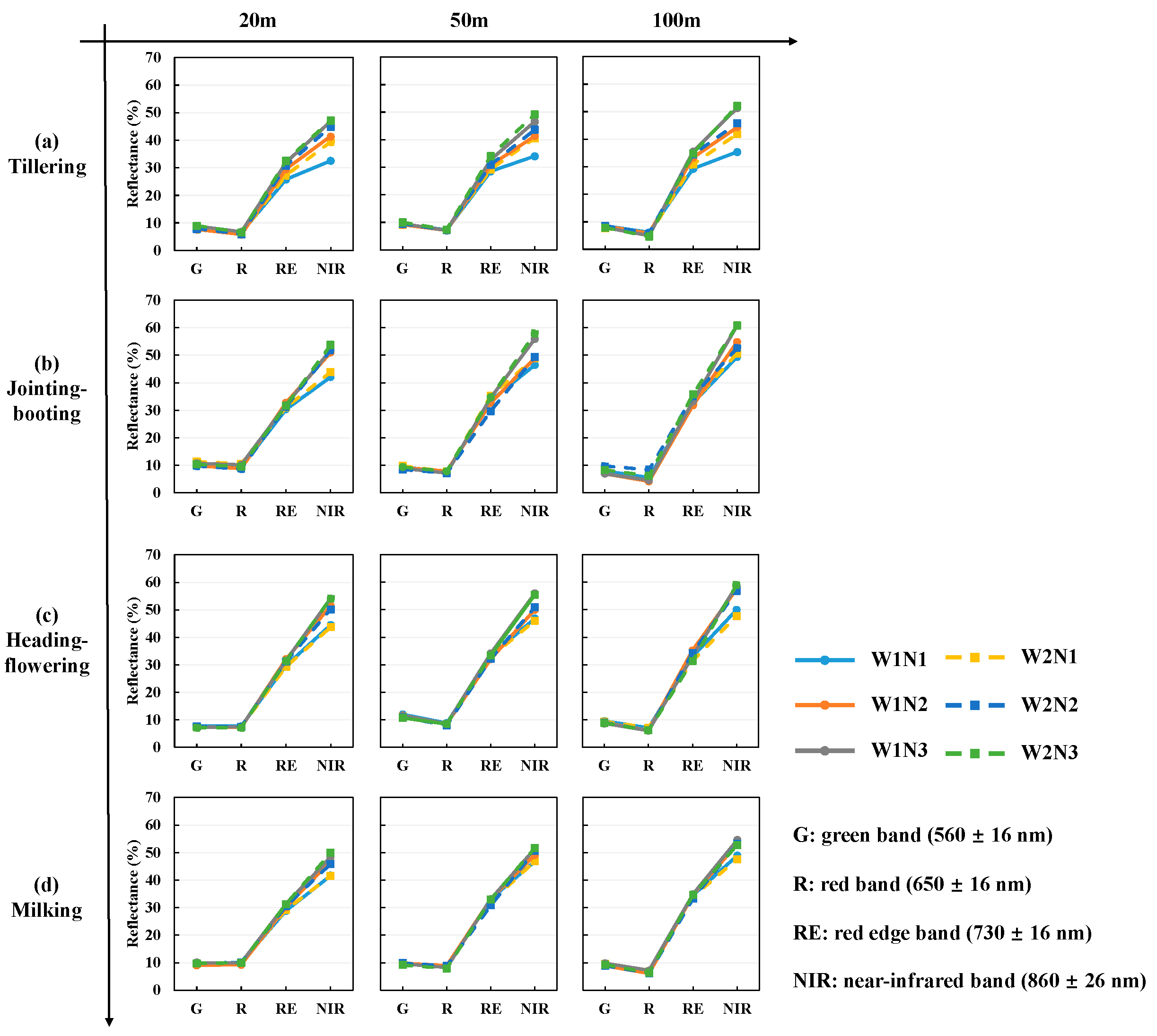
Figure 4 compares reflectance in four multispectral bands, G (560 nm), R (650 nm), RE (730 nm), and NIR (860 nm), measured at flight altitudes of 20, 50, and 100 m across rice growth stages. The G and R bands varied only slightly among treatments and growth stages. In particular, the R band showed the lowest reflectance and provided limited discrimination of differences induced by water and nitrogen treatments. By contrast, the RE and NIR bands were more responsive to changes in rice growth status and captured canopy differences associated with nitrogen application and irrigation regime. The NIR band showed the strongest temporal variation. Reflectance was relatively low at the late tillering stage, increased during the jointing–booting and heading–flowering stages, and then declined at the milking stage as the canopy senesced. This trajectory was consistent with the pattern observed in the near-infrared region of canopy hyperspectral data.

Figure 4. Average multispectral reflectance of rice canopy under different flight altitudes. (a–d) are UAV multispectral reflectance at the tillering, jointing–booting, heading–flowering and milking stages, respectively.

Table 3 presents the comparison between multispectral reflectance acquired at different flight altitudes and hyperspectral reflectance derived using corresponding spectral response functions. Among the three flight altitudes, 50 m produced the best overall agreement between multispectral reflectance and canopy spectra convolved with SRFs. Its overall RMSE was 5.085%, compared with 6.098% at 20 m and 5.908% at 100 m. For specific bands, the 50 m imagery had the lowest RMSE in G (1.535%), R (3.123%) and NIR (5.894%), whereas the RE band was closest at 20 m (4.688% versus 7.523% at 50 m).

Table 3. Consistency between UAV multispectral reflectance and canopy-SRF reflectance.

Altitude	Overall Accuracy of Four Bands			Single Band RMSE (%)
	RMSE (%)	R2corr	CCC	G	R	RE	NIR
20 m	6.098	0.9486	0.9465	1.937	5.310	4.688	9.739
50 m	5.085	0.9504	0.9674	1.535	3.123	7.523	5.894
100 m	5.908	0.9467	0.9516	2.493	4.797	6.542	8.223

3.3. Reconstruction Model Accuracy Under Different Data Simulation Methods

The average accuracy from the 10-fold cross-validation tests of the models based on MC and C-Vine methods is listed in Table 4. Overall, all models achieved relatively high mean CCC values (0.9256–0.9999), indicating overall agreement between reconstructed and reference spectra. However, clear differences in RMSE and SAM revealed variation in the recovery of absolute reflectance magnitude and spectral shape. On the C-vine dataset, cubic spline yielded the highest RMSE (8.037 ± 0.032%) and SAM (12.681 ± 0.025°). Among the machine learning models, SE-ResNet-Att achieved the lowest RMSE (0.287 ± 0.010%) and SAM (0.398 ± 0.008°) on this dataset. PLSR performed comparably, with an RMSE of 0.301 ± 0.009% and a slightly higher SAM of 0.416 ± 0.007°.

Table 4. Average reconstruction accuracy from 10-fold cross-validation of models based on different prior-knowledge data simulation methods.

Models	MC Method			C-Vine Method
	RMSE (%)	CCC	SAM (°)	RMSE (%)	CCC	SAM (°)
Cubic spline	5.450 ± 0.106	0.951	9.619 ± 0.078	8.037 ± 0.032	0.925	12.681 ± 0.025
PLL	2.681 ± 0.035	0.983	5.241 ± 0.078	6.508 ± 0.039	0.943	11.063 ± 0.054
PLSR	1.273 ± 0.019	0.996	2.201 ± 0.023	0.301 ± 0.009	1.000	0.416 ± 0.007
MLP	1.564 ± 0.025	0.994	2.617 ± 0.030	0.410 ± 0.007	1.000	0.490 ± 0.007
SE-ResNet-Att	1.100 ± 0.020	0.998	1.872 ± 0.021	0.287 ± 0.010	1.000	0.398 ± 0.008

Note: since the standard deviation of the CCC value was very small, it was not presented here.

The machine learning models consistently showed higher reconstruction accuracy on the C-vine dataset than on the MC dataset. For PLSR, MLP and SE-ResNet-Att, mean RMSE ranged from 0.287% to 0.410% under C-vine, compared with 1.100% to 1.564% under MC. The same pattern was observed for mean SAM, which ranged from 0.398° to 0.490° under C-vine and from 1.872° to 2.617° under MC. For these models, RMSE standard deviations were 0.007–0.010% under C-vine and 0.019–0.025% under MC, indicating limited variation across folds. In contrast, cubic spline and PLL performed better on the MC-generated dataset. Cubic spline yielded an RMSE of 5.450 ± 0.106% under MC, compared with 8.037 ± 0.032% under C-vine. For PLL, the corresponding RMSE values were 2.681 ± 0.035% and 6.508 ± 0.039%, respectively.

3.4. Reconstruction Model Accuracy Using Ground-Resampled and UAV Multispectral Inputs

The transferability of the reconstruction models was evaluated using ground-resampled canopy reflectance inputs at field scale and UAV multispectral inputs at UAV-field scale. Reconstruction accuracy at both scales is presented in Table 5 and Figure 5.

Table 5. Average reconstruction accuracy of models at field scale and UAV-field scale based on the full-prior data.

Models	Field Scale (n = 24)			UAV-Field Scale (n = 24)
	RMSE (%)	CCC	SAM (°)	RMSE (%)	CCC	SAM (°)
Cubic spline	12.509	0.879	17.155	9.484	0.917	13.896
PLL	6.024	0.964	9.750	6.977	0.946	10.657
PLSR	1.352	0.998	2.165	4.427	0.978	5.801
MLP	3.599	0.987	3.590	4.823	0.973	6.187
SE-ResNet-Att	1.966	0.996	2.710	4.298	0.980	5.446

Note: RMSE, CCC and SAM were calculated separately for each spectrum and averaged across the 24 treatment-stage spectra. Since the standard deviation of the CCC value is very small, it is not presented here.

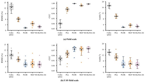
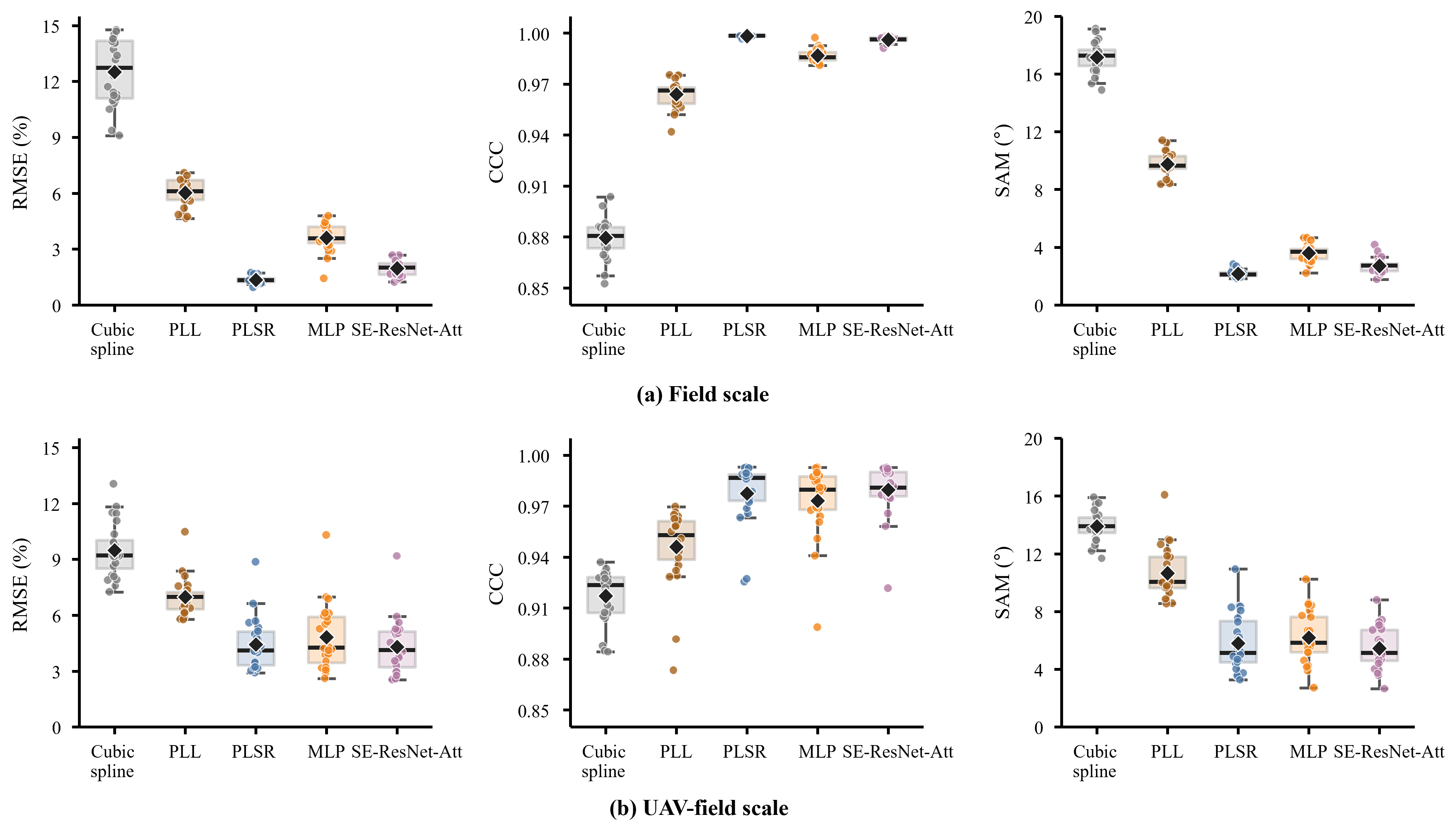
Figure 5. Box plots of reconstruction accuracy at field scale and UAV-field scale. (a) and (b) are evaluation metrics of models at field scale and UAV-field scale, respectively.

For field-scale validation, the reconstruction error increased relative to the simulated test set, but the machine learning models still clearly outperformed the deterministic baselines. PLSR achieved the best same-source performance, with an RMSE of 1.352%, CCC of 0.998, and SAM of 2.165°. MLP and SE-ResNet-Att obtained RMSE values of 3.599% and 1.966%, respectively, with corresponding CCC values of 0.987 and 0.996. By comparison, cubic spline and PLL produced much larger errors, with RMSE values of 12.509% and 6.024% and SAM values of 17.155° and 9.750°, respectively. The boxplots further showed that PLSR had a compact distribution of RMSE and SAM across the 24 field samples, whereas SE-ResNet-Att showed slightly larger sample-to-sample variability.

When 50 m UAV multispectral inputs were used for UAV-to-ground transfer validation, the performance of all machine learning models declined. The RMSE values of PLSR, MLP, and SE-ResNet-Att increased to 4.427%, 4.823%, and 4.298%, respectively. Their SAM values also increased to 5.801°, 6.187°, and 5.446°, respectively, while CCC values remained high at approximately 0.973–0.980. Among the machine learning models, SE-ResNet-Att achieved the lowest RMSE and SAM under the UAV-field scale, suggesting a relatively stronger ability to tolerate input mismatch, although the RMSE difference from PLSR was only 0.129%.

To further evaluate the generalization of the reconstruction models across growth stages within this study, leave-one-growth-stage-out validation was performed. The mean reconstruction accuracy across the four folds is summarized in Table 6, while the results for individual folds are provided in Appendix A Table A1 and Table A2.

Table 6. Average reconstruction accuracy across four held-out stages at field and UAV-field scales.

Models	Field Scale (n = 6 Per Fold)			UAV-Field Scale (n = 6 Per Fold)
	RMSE (%)	CCC	SAM (°)	RMSE (%)	CCC	SAM (°)
Cubic spline	12.509 ± 1.872	0.879	17.155 ± 0.925	9.484 ± 1.008	0.917	13.896 ± 0.698
PLL	6.024 ± 0.733	0.964	9.750 ± 0.626	6.977 ± 0.578	0.946	10.657 ± 1.064
PLSR	1.604 ± 0.191	0.998	2.440 ± 0.523	4.368 ± 0.681	0.978	5.671 ± 1.111
MLP	3.257 ± 0.753	0.989	3.382 ± 0.510	4.871 ± 1.369	0.972	6.324 ± 1.040
SE-ResNet-Att	1.905 ± 0.230	0.996	2.604 ± 0.234	4.340 ± 1.087	0.979	5.421 ± 0.993

Note: RMSE, CCC and SAM were calculated separately for each spectrum and averaged across the 24 treatment-stage spectra. Since the standard deviation of the CCC value was very small, it was not presented here.

Overall, the machine learning models achieved lower mean RMSE and SAM than cubic spline and PLL at both validation scales. In field-scale validation, PLSR achieved the lowest mean RMSE (1.604% ± 0.191%) and SAM (2.440 ± 0.523°). Its mean CCC was also the highest (0.998). SE-ResNet-Att ranked second, with an RMSE of 1.905% ± 0.230% and SAM of 2.604 ± 0.234°. MLP yielded a higher RMSE of 3.257% ± 0.753%. Cubic spline and PLL yielded RMSE values of 12.509% ± 1.872% and 6.024% ± 0.733%, respectively.

In UAV-field validation, SE-ResNet-Att achieved the lowest mean RMSE (4.340% ± 1.087%) and SAM (5.421 ± 0.993°). It also yielded the highest mean CCC of 0.979. PLSR showed comparable mean accuracy, with an RMSE of 4.368% ± 0.681% and SAM of 5.671 ± 1.111°. MLP showed higher errors, with an RMSE of 4.871% ± 1.369% and SAM of 6.324 ± 1.040°. Cubic spline and PLL yielded RMSE values of 9.484% ± 1.008% and 6.977% ± 0.578%, respectively. Although SE-ResNet-Att achieved a slightly lower mean RMSE than PLSR, PLSR showed less variation in RMSE among the four held-out stages. Conversely, SE-ResNet-Att showed slightly less variation in SAM, indicating that the relative variability depended on the evaluation metric.

Detailed model rankings varied with the held-out growth stage and validation scale. At field scale, SE-ResNet-Att performed best at tillering, whereas PLSR performed best at the other three stages. At UAV-field scale, SE-ResNet-Att performed best at tillering, jointing–booting and milking, while PLSR performed best at heading–flowering. However, the accuracy differences between PLSR and SE-ResNet-Att were relatively small across growth stages. Differences in RMSE ranged from 0.191% to 0.540% at field scale and from 0.129% to 0.668% at UAV-field scale.

3.5. Reconstructed Red-Edge Position and Exploratory Relationships with Canopy Traits

To evaluate the fidelity of the reconstructed red-edge features, REP extracted from the SE-ResNet-Att spectra reconstructed using 50 m UAV inputs was compared with REP extracted from ground measured canopy spectra (Appendix A Table A3). Across the 24 treatment-stage pairs, ground measured REP ranged from 722 to 734 nm, whereas UAV-reconstructed REP ranged from 702 to 725 nm. The two sets of REP values were correlated (Pearson r = 0.928), but reconstructed REP was consistently displaced toward shorter wavelengths. The differences ranged from −20 to −9 nm, with a mean difference (reconstructed minus measured REP) of −12.04 nm.

Both spectral sources showed similar overall patterns across growth stages and nitrogen treatments. Mean REP across the six treatments increased from tillering to heading–flowering and subsequently decreased at milking. When averaged across growth stages, REP increased from N1 to N3 under both irrigation regimes for both spectra. The lower REP values in the N1 treatments, particularly during the tillering stage, showed a shift in the red-edge transition toward shorter wavelengths under sparse canopy development. These results indicate that the reconstruction reproduced broad patterns of REP variation, although its absolute wavelength estimates remained biased.

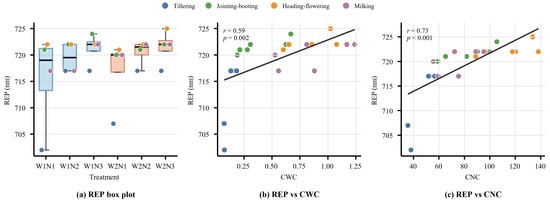
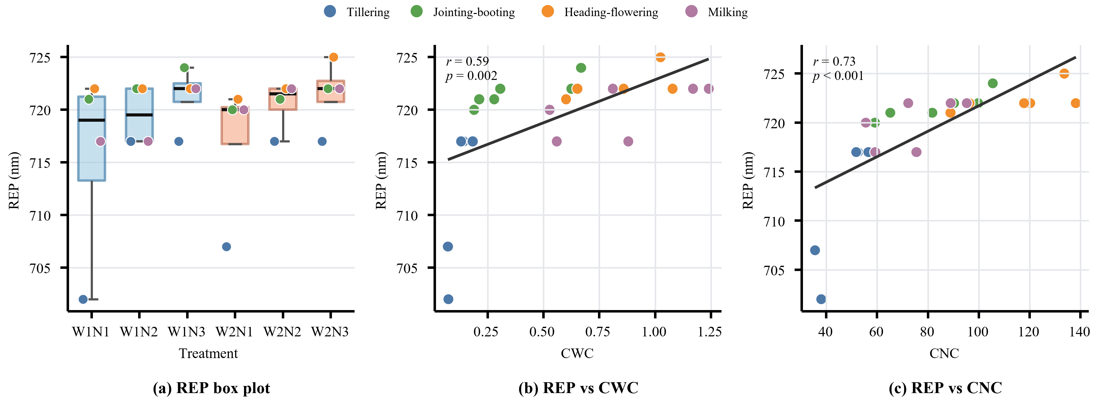
In the exploratory analysis, the pooled reconstructed REP was positively associated with both CWC and CNC, with a stronger association for CNC. As shown in Figure 6, REP showed a correlation with CWC (Pearson r = 0.589), while its correlation with CNC was stronger (Pearson r = 0.727). The rank-based correlations showed the same pattern, with Spearman coefficients of 0.764 for CWC and 0.895 for CNC.

Figure 6. REP retrieved from the reconstructed spectra reflectance curve and its exploratory relationships with CWC and CNC. Note: The correlations and nominal p-values shown were calculated from pooled data without adjustment for repeated measurements of the same plots across growth stages.

To account for growth stage, REP and each canopy trait were first centered on their respective stage means, and Pearson correlations were calculated between the centered values. To additionally account for LAI while allowing its relationships to vary among stages, REP and each trait were further separately regressed on LAI within each growth stage, with a stage-specific intercept and slope. Pearson correlations were then calculated between the corresponding residuals. After adjustment for growth stage, the REP–CWC and REP–CNC correlations decreased to 0.367 and 0.497, respectively. Further adjustment using stage-specific LAI slopes reduced these correlations to 0.110 and 0.203. Since LAI was included in the calculations of CWC and CNC, it was strongly correlated with both traits (Pearson r = 0.947 and 0.859, respectively). These results suggest that the pooled REP associations partly reflected variation shared with canopy development, particularly because both canopy traits contain LAI as a multiplicative component.

The differences between irrigation regimes were modest. CWC under W2 was 0.5–10.6% lower than under W1. Although mean REP was 0.92 nm higher under W2, individual differences ranged from −2 to 5 nm. REP therefore showed no consistent directional response to irrigation regimes. This is because the lower irrigation threshold of 80% under W2 did not induce severe water stress for rice, resulting in only minor changes in REP. The increase in mean REP with nitrogen application under both irrigation regimes was consistent with its stronger association with CNC. Nevertheless, the weak correlations after stage-specific LAI adjustment indicate that these relationships largely overlapped with canopy development and provide limited evidence of independent water or nitrogen sensitivity.

4. Discussion

4.1. The Effect of Prior Knowledge on Reconstruction Accuracy

Crop growth parameters are inherently highly correlated and vary across growth stages. However, previous studies typically employed uniform distributions with MC methods to generate datasets. This approach assumes parameter independence, often resulting in biologically implausible parameter combinations (e.g., high LAI paired with extremely low Cab) and thereby introducing noise into the spectral dataset. Constructing a joint distribution function for these parameters using a C-Vine copula effectively preserves their intrinsic biological correlations, ensuring that the simulated spectral data more accurately reflect real-world conditions.

Compared with the MC method, the mean wavelength-wise standard deviation of simulated reflectance decreased from 6.88% to 2.89% points under the C-vine method. This narrower distribution of target spectra can make the reconstruction task easier and may partly explain the lower errors of the machine learning models. While, the poorer performance of cubic spline and PLL under the C-vine prior does not indicate a lower quality of the C-vine dataset. These two methods are deterministic curve-fitting baselines that rely on fixed spectral-shape assumptions and cannot exploit the joint distribution of canopy parameters. The observed gains in machine learning models performance should therefore be interpreted as conditional on the adopted prior and evaluation domain.

4.2. Why Does Greater Model Complexity Provide Limited Accuracy Gains?

To further examine the contribution of the proposed network components, an ablation experiment was conducted on the 24 measured canopy spectra. The ResNet, SE-ResNet and SE-ResNet-Att ablation models used the same final full-prior training and evaluation protocol. All these models were evaluated against the same 24 measured canopy spectra using the same ground SRF-resampled inputs and 50 m UAV multispectral inputs. The measured reference and all reconstructed spectra were smoothed using the selected S–G filter before calculating the evaluation metrics.

The ablation results showed that adding the SE module alone did not improve the reconstruction accuracy. Under the UAV-field validation setting, the ResNet model achieved an RMSE of 4.381%, CCC of 0.979, and SAM of 5.692°, whereas SE-ResNet produced a slightly higher RMSE of 4.475% and SAM of 5.921°. After introducing the input attention module, SE-ResNet-Att reduced the RMSE to 4.298% and SAM to 5.446°, indicating that attention partially compensated for the degradation caused by the SE module (Table 7). However, the improvement over the plain ResNet remained small, suggesting that the additional recalibration modules provided limited gains under field transfer conditions.

Table 7. Average reconstruction accuracy of SE-ResNet-Att ablation test at field scale and UAV-field scale.

Models	SE Module	Attention Module	Field Scale (n = 24)			UAV-Field Scale (n = 24)
			RMSE (%)	CCC	SAM (°)	RMSE (%)	CCC	SAM (°)
ResNet	NO	NO	2.075	0.996	2.885	4.381	0.979	5.692
SE-ResNet	YES	NO	2.644	0.993	2.892	4.475	0.978	5.921
SE-ResNet-Att	YES	YES	1.966	0.996	2.710	4.298	0.980	5.446

Table 7. Average reconstruction accuracy of SE-ResNet-Att ablation test at field scale and UAV-field scale.

Models	SE Module	Attention Module	Field Scale (n = 24)			UAV-Field Scale (n = 24)
			RMSE (%)	CCC	SAM (°)	RMSE (%)	CCC	SAM (°)
ResNet	NO	NO	2.075	0.996	2.885	4.381	0.979	5.692
SE-ResNet	YES	NO	2.644	0.993	2.892	4.475	0.978	5.921
SE-ResNet-Att	YES	YES	1.966	0.996	2.710	4.298	0.980	5.446

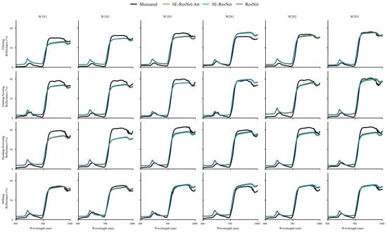
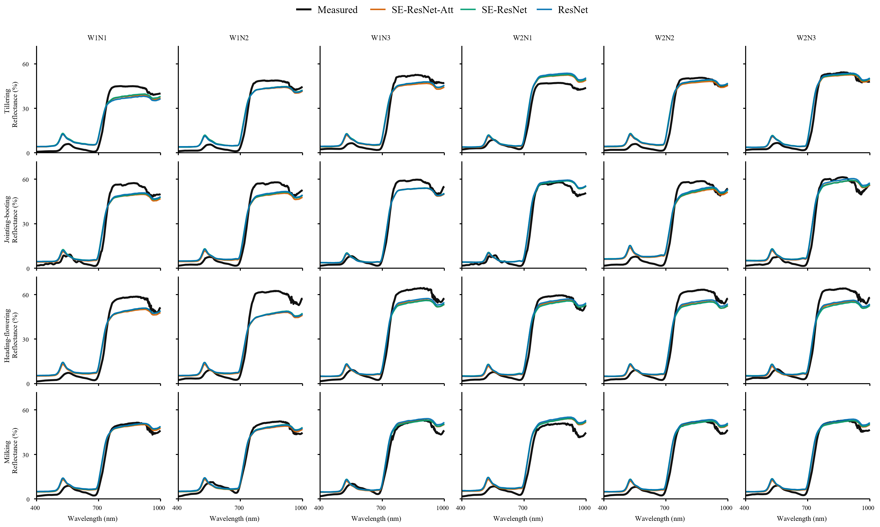
Figure 7 compares measured canopy hyperspectral reflectance with spectra reconstructed from UAV multispectral observations and further supports these results. All three models reproduced the overall red-edge rise and near-infrared plateau, but their reconstructed curves were highly similar. The main errors were not local oscillations that could be corrected by a deeper network, but systematic deviations in reflectance magnitude, especially in the NIR plateau and visible region for some growth stages. This indicated that the limiting factor was not network expressiveness alone, but the information constraint imposed by reconstructing 601 narrow bands from only four broad multispectral inputs.

Figure 7. Comparison of measured canopy hyperspectral reflectance with spectra reconstructed from UAV multispectral observations using different ablation models.

Several factors may limit the benefit of greater network complexity. First, the reconstruction from four-band to hyperspectral is intrinsically underdetermined, therefore additional parameters cannot recover spectral details that are not encoded in the input bands [25]. Second, the network was trained on simulated spectral reflectance data based on PROSAIL-D, whereas the 24 measured spectra include canopy structural effects, sensor noise, illumination differences, and scale mismatch. A more flexible model may therefore learn simulation-specific nonlinear patterns that do not transfer well to field observations. The relative performance of PLSR and SE-ResNet-Att depended on the source of the multispectral inputs. In both the full-prior and leave-one-growth-stage-out evaluations, PLSR achieved lower RMSE with ground-resampled inputs, while SE-ResNet-Att showed a small advantage with UAV inputs. MLP consistently produced the largest errors among the three learned models. These results highlight the effectiveness of PLSR as a relatively simple reconstruction method, with the advantage of the more complex SE-ResNet-Att architecture limited to a modest reduction in UAV-field error.

Overall, the ablation analysis indicated that the SE module alone did not improve UAV-field accuracy. Input attention reduced errors relative to SE-ResNet, but the improvement over ResNet remained small. The results support using reconstructed spectra to examine broad spectral patterns within the evaluated domain, while providing limited evidence that additional network modules consistently improve transfer to field observations.

4.3. Application Boundaries of Spectral Features After Reconstruction

Reconstructing continuous spectra extends four-band UAV observations into wavelength-resolved estimates that support the examination of canopy spectral shape and derived features such as REP. The recovered red-edge rise and near-infrared plateau provide a basis for exploring seasonal canopy development, but agreement in broad spectral patterns does not ensure the accuracy of individual features. For REP, small changes in the reconstructed red-edge shape can shift the maximum first derivative. Previous rice studies have also shown that REP–CNC relationships depend on the extraction algorithm, with multiple derivative peaks complicating conventional maximum-derivative estimates [2]. In the present experiment, although both reconstructed and measured REP were obtained using the same extraction method, the REP correlation coexisted with an obvious mean bias toward shorter wavelengths of −12.04 nm. The observed displacement of 9–20 nm was comparable to or larger than the full 12 nm range of measured REP (722–734 nm). Therefore, reconstructed REP cannot replace measured REP in applications requiring accurate absolute wavelength estimates. The REP discrepancy may partly arise from observation-scale differences between UAV multispectral reflectance and the ground measurements. The SRF-consistency term (L_SRF) in the loss function constrained the reconstructed spectra to reproduce the input reflectance of the red-edge band (730 nm) after SRF integration. However, this constraint does not uniquely determine the band spectral shape or the wavelength of maximum slope.

The stronger pooled REP–CNC association and the increase in REP with nitrogen application suggest that reconstructed REP is associated with nitrogen-related canopy variation. However, adjustment for growth stage and stage-specific LAI relationships reduced the correlations with CWC and CNC to 0.110 and 0.203, respectively. Because both traits contain LAI as a multiplicative component, these associations partly reflected canopy development, with limited evidence of independent water or nitrogen sensitivity.

The application boundaries arise from both the spectral information available and the conditions represented in the experiment [26]. Four multispectral bands constrain broad spectral shape, while finer red-edge details depend partly on the reconstruction prior. Local reconstruction errors can therefore shift derivative-based features such as REP, and remaining UAV-field discrepancies can obscure small irrigation-related differences. These limitations explain why the recovery of broad spectral patterns does not necessarily support accurate trait retrieval or irrigation discrimination. Reconstructed REP should consequently be treated as a candidate descriptor for canopy monitoring, with its relative patterns presently supported only within this experiment. Quantitative applications of reconstructed REP require validation against measured spectral features and independent plant water and nitrogen measurements across a wider range of field conditions.

4.4. Reconstruction Accuracy Under Limited Spectral Coverage

Regional RMSE and RRMSE were reported in Appendix A Table A4 and Table A5. In general, the comparison indicated that the reconstruction accuracy depended not only on spectral coverage, but also on reflectance magnitude and spectral shape. Under the full-prior setting, the three learning-based models showed their largest UAV-field-scale RMSE in the red-edge (5.670–6.475%), but their largest RRMSE in the blue region (95.3–108.5%). Strong pigment absorption produces low blue reflectance, making small absolute errors substantial relative to the signal [1]. For SE-ResNet-Att, blue-region RMSE increased from 0.820% at field scale to 2.611% at UAV-field scale, corresponding to RRMSE values of 31.0% and 98.7%. The absence of a blue input also makes reconstruction dependent on relationships with the observed bands. Green and red inputs may provide additional constraints within 521–679 nm, consistent with the lower relative errors in this interval, although band-integrated measurements cannot fully determine narrow-band spectral shape.

The reconstruction of the red-edge spectra remained challenging despite the availability of a red-edge channel (with central band of 730 nm). Its steep transition responds to pigment content and canopy structure, so small errors in transition position or slope can produce substantial reflectance deviations [27]. PLSR red-edge RMSE increased from 0.718% with ground-resampled inputs to 6.153% with UAV inputs, whereas SE-ResNet-Att increased from 2.881% to 5.670%. These differences indicate greater sensitivity of red-edge reconstruction to the input source in this experiment.

At UAV-field scale, the machine learning models achieved lower reconstruction errors over 880–1000 nm than over 761–879 nm, despite the absence of an additional input band at longer wavelengths. This pattern may reflect the shared physical controls on NIR reflectance. Leaf scattering and canopy structure influence the broad reflectance level across both intervals, providing a basis for estimating longer-wavelength reflectance from the observed NIR band. These spectral relationships are represented in the PROSAIL simulations, while the C-Vine priors retain dependencies among the physiological and structural variables used to generate them. Learning these relationships may therefore help constrain reconstruction beyond the measured bands.

The accuracy differences between field and UAV-field scale also reflect acquisition conditions. Ground-resampled inputs and reference spectra share the same measurements, whereas UAV inputs represent independently acquired vegetation-pixel averages within plot ROIs. Differences in calibration, illumination, viewing geometry and spatial sampling can change the input reflectance, as demonstrated in previous UAV rice studies [3]. Such differences can affect both the NIR reflectance level and the red-to-NIR contrast used to reconstruct the red edge, providing plausible explanations for the increased errors in these intervals. The 970 nm evaluation further examined reflectance at a water-sensitive wavelength. Under the full-prior dataset, SE-ResNet-Att achieved the lowest 970 nm RMSE at both field and UAV-field scales (1.791% and 4.014%), with RRMSE values of 3.7% and 8.4%. These results support the recovery of reflectance at the absorption wavelength, potentially aided by physiological relationships (especially the Cw) in the training data. Absorption depth additionally depends on the surrounding continuum.

Further leave-one-growth-stage-out validation results indicated that sensitivity to excluding a growth stage varied with the model and spectral feature, while large blue-region relative errors (RRMSE) and red-edge absolute errors (RMSE) remained the principal weaknesses under UAV inputs.

4.5. Limitations and Future Directions

Several limitations should be acknowledged. First, the measured validation dataset contained only 24 treatment-level mean spectra from a single field experiment. These spectra were derived from 10 plots observed over four stages, with unbalanced replication due to the limited field area, which limits the evaluation of model generalization across cultivars, years, sites and management conditions. Second, the C-vine priors were fitted to physiological measurements from the same experiment used for spectral validation. Leave-one-growth-stage-out validation excluded the target-stage prior but assessed transfer only among stages within this experiment. Moreover, the lower errors obtained with the C-Vine method may therefore partly reflect its narrower spectral variability and cannot be attributed solely to improved representation of parameter dependence. Third, the data simulation process used fixed solar zenith, viewing zenith and relative azimuth angles for simulation convenience. However, the fixed geometry did not represent all acquisition dates, and this approximation may contribute to differences between simulated and measured reflectance. Moreover, the dry and wet soil factor does not explicitly represent a standing-water layer or its directional optical effects. This limitation is particularly relevant to flooded W1 plots when canopy cover is sparse at the tillering stage, but the effects of the mixed background tend to diminish as the canopy develops [20]. Nevertheless, these factors remain potential sources of error.

Future studies should evaluate the framework on independent fields, years, and rice cultivars, and test spectral and REP calibration on observations not used to develop the prior or fit the calibration. In addition, uncertainty estimation should be further strengthened so that reconstructed spectra and extracted red-edge features can be used with clear confidence boundaries.

5. Conclusions

This study developed and evaluated a physically guided framework for reconstructing continuous rice canopy reflectance from four-band UAV multispectral observations. The main conclusions are as follows:

(1)

Spectral consistency was strongly affected by measurement scale. Leaf and canopy spectra preserved similar overall vegetation spectral patterns, with mean R² corr values of 0.964–0.981 and CCC values of 0.943–0.979. Among the three tested flight altitudes, 50 m provided the closest overall agreement between UAV multispectral reflectance and ground canopy spectra, with an RMSE of 5.085%.

(2)

The construction of the spectral prior substantially affected reconstruction accuracy. Compared with the Monte Carlo sampling for PROSAIL-D, the C-Vine method reduced the RMSE of the machine learning models from 1.100 to 1.564% to 0.287–0.410%.

(3)

Model performance varied across validation scales, and greater network complexity provided limited gains. PLSR performed best in field-scale validation with ground-resampled inputs (RMSE, 1.352%), whereas SE-ResNet-Att achieved the lowest RMSE (4.298%) at UAV-field scale. Leave-one-growth-stage-out validation yielded similar mean UAV-field errors for SE-ResNet-Att and PLSR (RMSE of 4.340% and 4.368%). Without real multispectral observation constraints, the relative error of blue-region and absolute error of red-edge remained prominent under UAV inputs.

(4)

The ablation experiment showed that adding the SE module alone did not improve UAV-field reconstruction accuracy. Input attention reduced errors relative to SE-ResNet, but the improvement remained small. These results indicate that reconstruction was mainly constrained by the limited information in four multispectral bands and the observation scale.

(5)

The reconstructed spectra preserved broad red-edge and near-infrared patterns, but the reconstructed red-edge position (REP) remained shifted toward shorter wavelengths (mean bias of −12.04 nm). The reconstructed REP was exploratorily correlated with canopy water content (Pearson r = 0.589) and canopy nitrogen content (Pearson r = 0.727). However, these correlations decreased to 0.110 and 0.203 after adjustment for growth stage and LAI relationships, indicating limited evidence of independent water or nitrogen sensitivity. The findings are limited to the present experiment. Model performance across independent fields, years, and rice cultivars requires further validation.

References

- Féret, J.-B.; Gitelson, A.A.; Noble, S.D.; Jacquemoud, S. PROSPECT-D: Towards Modeling Leaf Optical Properties through a Complete Lifecycle. Remote Sens. Environ. 2017, 193, 204–215. [Google Scholar] [CrossRef] [Scilit]
- Tian, Y.; Yao, X.; Yang, J.; Cao, W.; Zhu, Y. Extracting Red Edge Position Parameters from Ground- and Space-Based Hyperspectral Data for Estimation of Canopy Leaf Nitrogen Concentration in Rice. Plant Prod. Sci. 2011, 14, 270–281. [Google Scholar] [CrossRef] [Scilit]
- Luo, S.; Jiang, X.; Yang, K.; Li, Y.; Fang, S. Multispectral Remote Sensing for Accurate Acquisition of Rice Phenotypes: Impacts of Radiometric Calibration and Unmanned Aerial Vehicle Flying Altitudes. Front. Plant Sci. 2022, 13, 958106. [Google Scholar] [CrossRef] [Scilit] [PubMed]
- Zhu, H.; Huang, Y.; An, Z.; Zhang, H.; Han, Y.; Zhao, Z.; Li, F.; Zhang, C.; Hou, C. Assessing Radiometric Calibration Methods for Multispectral UAV Imagery and the Influence of Illumination, Flight Altitude and Flight Time on Reflectance, Vegetation Index and Inversion of Winter Wheat AGB and LAI. Comput. Electron. Agric. 2024, 219, 108821. [Google Scholar] [CrossRef] [Scilit]
- Arad, B.; Ben-Shahar, O. Sparse Recovery of Hyperspectral Signal from Natural RGB Images. In Proceedings of the Computer Vision—ECCV 2016; Leibe, B., Matas, J., Sebe, N., Welling, M., Eds.; Springer International Publishing: Cham, Switzerland, 2016; pp. 19–34. [Google Scholar]
- Alvarez-Gila, A.; Van De Weijer, J.; Garrote, E. Adversarial Networks for Spatial Context-Aware Spectral Image Reconstruction from RGB. In Proceedings of the 2017 IEEE International Conference on Computer Vision Workshops (ICCVW), Venice, Italy, 22–29 October 2017; pp. 480–490. [Google Scholar]
- Shi, Z.; Chen, C.; Xiong, Z.; Liu, D.; Wu, F. HSCNN+: Advanced CNN-Based Hyperspectral Recovery from RGB Images. In Proceedings of the 2018 IEEE/CVF Conference on Computer Vision and Pattern Recognition Workshops (CVPRW), Salt Lake City, UT, USA, 18–22 June 2018; pp. 1052–10528. [Google Scholar]
- Togeiro de Alckmin, G.; Kooistra, L.; Rawnsley, R.; de Bruin, S.; Lucieer, A. Retrieval of Hyperspectral Information from Multispectral Data for Perennial Ryegrass Biomass Estimation. Sensors 2020, 20, 7192. [Google Scholar] [CrossRef] [Scilit] [PubMed]
- Wang, J.; Belwalkar, A.; Meyer, S.T.; Li, F.; Herrmann, I.; Yu, K. UAV Multispectral to Hyperspectral Reconstruction Based on Deep Learning and Radiative Transfer Models for Crop Nitrogen Monitoring. Int. J. Appl. Earth Obs. Geoinf. 2026, 150, 105364. [Google Scholar] [CrossRef] [Scilit]
- Yue, J.; Li, T.; Feng, H.; Fu, Y.; Liu, Y.; Tian, J.; Yang, H.; Yang, G. Enhancing Field Soil Moisture Content Monitoring Using Laboratory-Based Soil Spectral Measurements and Radiative Transfer Models. Agric. Commun. 2024, 2, 100060. [Google Scholar] [CrossRef] [Scilit]
- Chakhvashvili, E.; Siegmann, B.; Muller, O.; Verrelst, J.; Bendig, J.; Kraska, T.; Rascher, U. Retrieval of Crop Variables from Proximal Multispectral UAV Image Data Using PROSAIL in Maize Canopy. Remote Sens. 2022, 14, 1247. [Google Scholar] [CrossRef] [Scilit] [PubMed]
- Zérah, Y.; Valero, S.; Inglada, J. Physics-Constrained Deep Learning for Biophysical Parameter Retrieval from Sentinel-2 Images: Inversion of the PROSAIL Model. Remote Sens. Environ. 2024, 312, 114309. [Google Scholar] [CrossRef] [Scilit]
- Yu, F.; Bai, J.; Fang, J.; Guo, S.; Zhu, S.; Xu, T. Integration of a Parameter Combination Discriminator Improves the Accuracy of Chlorophyll Inversion from Spectral Imaging of Rice. Agric. Commun. 2024, 2, 100055. [Google Scholar] [CrossRef] [Scilit]
- Wang, J.; Lopez-Lozano, R.; Weiss, M.; Buis, S.; Li, W.; Liu, S.; Baret, F.; Zhang, J. Crop Specific Inversion of PROSAIL to Retrieve Green Area Index (GAI) from Several Decametric Satellites Using a Bayesian Framework. Remote Sens. Environ. 2022, 278, 113085. [Google Scholar] [CrossRef] [Scilit]
- Yin, F.; Lewis, P.E.; Gómez-Dans, J.L.; Weiß, T. Archetypal Crop Trait Dynamics for Enhanced Retrieval of Biophysical Parameters from Sentinel-2 MSI. Remote Sens. Environ. 2025, 318, 114510. [Google Scholar] [CrossRef] [Scilit]
- Aas, K.; Czado, C.; Frigessi, A.; Bakken, H. Pair-Copula Constructions of Multiple Dependence. Insur. Math. Econ. 2009, 44, 182–198. [Google Scholar] [CrossRef] [Scilit]
- Wan, L.; Zhu, J.; Du, X.; Zhang, J.; Han, X.; Zhou, W.; Li, X.; Liu, J.; Liang, F.; He, Y.; et al. A Model for Phenotyping Crop Fractional Vegetation Cover Using Imagery from Unmanned Aerial Vehicles. J. Exp. Bot. 2021, 72, 4691–4707. [Google Scholar] [CrossRef] [Scilit] [PubMed]
- Wan, L.; Cen, H.; Zhu, J.; Zhang, J.; Zhu, Y.; Sun, D.; Du, X.; Zhai, L.; Weng, H.; Li, Y.; et al. Grain Yield Prediction of Rice Using Multi-Temporal UAV-Based RGB and Multispectral Images and Model Transfer—A Case Study of Small Farmlands in the South of China. Agric. For. Meteorol. 2020, 291, 108096. [Google Scholar] [CrossRef] [Scilit]
- Chen, Q.; Zheng, B.; Chen, T.; Chapman, S.C. Integrating a Crop Growth Model and Radiative Transfer Model to Improve Estimation of Crop Traits Based on Deep Learning. J. Exp. Bot. 2022, 73, 6558–6574. [Google Scholar] [CrossRef] [Scilit] [PubMed]
- Wu, T.; Zheng, J.; Cheng, M.; Liu, K.; Jiao, X. Physics-Informed and Prior-Data Driven: A Hybrid Stacking Framework for Rice Growth Parameter Inversion. J. Integr. Agric. 2026. Epub ahead of print. [Google Scholar] [CrossRef] [Scilit]
- Jacquemoud, S.; Baret, F. PROSPECT: A Model of Leaf Optical Properties Spectra. Remote Sens. Environ. 1990, 34, 75–91. [Google Scholar] [CrossRef] [Scilit]
- Wan, L.; Zhang, J.; Dong, X.; Du, X.; Zhu, J.; Sun, D.; Liu, Y.; He, Y.; Cen, H. Unmanned Aerial Vehicle-Based Field Phenotyping of Crop Biomass Using Growth Traits Retrieved from PROSAIL Model. Comput. Electron. Agric. 2021, 187, 106304. [Google Scholar] [CrossRef] [Scilit]
- Savitzky, A.; Golay, M.J. Smoothing and Differentiation of Data by Simplified Least Squares Procedures. Anal. Chem. 1964, 36, 1627–1639. [Google Scholar] [CrossRef] [Scilit]
- Lin, L.I.-K. A Concordance Correlation Coefficient to Evaluate Reproducibility. Biometrics 1989, 45, 255–268. [Google Scholar] [CrossRef] [Scilit]
- Wang, B.; Li, K.; Sheng, Q.; Li, J.; Zhang, Y.; Ling, X.; Liu, X.; Guo, Y.; Wang, Y.; Zhu, Y. A Physics-Based Feature XGBoost Model for Frozen Ground Surface Reflectance Reconstruction on the Tibetan Plateau. IEEE Trans. Geosci. Remote Sens. 2026, 64, 4301317. [Google Scholar] [CrossRef] [Scilit]
- Bhadra, S.; Sagan, V.; Sarkar, S.; Braud, M.; Mockler, T.C.; Eveland, A.L. PROSAIL-Net: A Transfer Learning-Based Dual Stream Neural Network to Estimate Leaf Chlorophyll and Leaf Angle of Crops from UAV Hyperspectral Images. ISPRS J. Photogramm. Remote Sens. 2024, 210, 1–24. [Google Scholar] [CrossRef] [Scilit]
- Delegido, J.; Verrelst, J.; Meza, C.M.; Rivera, J.P.; Alonso, L.; Moreno, J. A Red-Edge Spectral Index for Remote Sensing Estimation of Green LAI over Agroecosystems. Eur. J. Agron. 2013, 46, 42–52. [Google Scholar] [CrossRef] [Scilit]
Disclaimer/Publisher’s Note: The statements, opinions and data contained in all publications are solely those of the individual author(s) and contributor(s) and not of MDPI and/or the editor(s). MDPI and/or the editor(s) disclaim responsibility for any injury to people or property resulting from any ideas, methods, instructions or products referred to in the content. |
© 2026 by the authors. Licensee MDPI, Basel, Switzerland. This article is an open access article distributed under the terms and conditions of the Creative Commons Attribution (CC BY) license.