


Abstract
Evaluating G × E interactions is key to plant breeding, but models like AMMI struggle with complex non-linear dynamics. This study combines Machine Learning (ML) algorithms with local additive SHAP decomposition to model the G × E interaction. A maize Grain Yield (GY) dataset from CIMMYT was used, containing nine genotypes evaluated across 20 environments. Mean GY ranged from 2652.00 kg ha−1 (Environment 19) to 7516.00 kg ha−1 (Environment 12), with Genotype 6 (G6) being the highest GY (5330.17 kg ha−1). According to the AMMI Stability Value (ASV), G7 and G3 were identified as the most stable genotypes despite their relatively low grain yield. In contrast, G6, the highest-yielding genotype, was ranked only fourth by ASV but achieved the top position in both the SHAP SSI and SHAP Effect metrics. These findings indicate that the environmental variation reflects a predictable non-linear responsiveness rather than stochastic instability. A high Spearman correlation was captured between GY per se and the SHAP Effect (, p < 0.0001), while the SHAP Stability metric showed a weak association with traditional linear measures with ASV, p = 0.2216). The ML-SHAP approach presents itself as an interesting and complementary tool in breeding, allowing one to better understand the complex and non-linear G × E interaction.
1. Introduction
The evaluation of genotype-by-environment (G × E) interaction and the selection of stable and responsive genotypes are fundamental steps in plant breeding programs [1]. For the analysis of multi-environment trials, linear and bilinear models are frequently employed, such as AMMI [2] and GGE Biplot [3]. These models apply singular value decomposition to the interaction matrix, allowing for the visual interpretation of its patterns via biplots [4,5].
Although these methodologies allow for the decomposition of multiplicative interaction effects into orthogonal interaction principal component axes (IPCAs), their mathematical structure assumes that genotype responses to environmental variations can be approximated by linear combinations of latent variables [6]. In practice, however, biological phenomena often involve complex, non-linear interactions that are difficult for classical multivariate models to capture [6]. In complex and non-linearity scenarios, the residuals of bilinear models, such as AMMI, tend to inflate, resulting in less accurate estimates of adaptability and stability. Consequently, the selection and discarding process for genotypes exhibiting complex response dynamics is compromised.
Alternatively, the application of Machine Learning (ML) algorithms, such as Random Forest, has been explored in prediction due to their ability to model complex multidimensional interactions without requiring any statistical assumptions [7]. Despite their demonstrated predictive potential, the routine adoption of these models in genetic breeding faces constraints due to the difficulty of directly interpreting their internal parameters [8]. Unlike classical approaches, ML techniques do not generate regression coefficients or direct scores per factor level [9], which limits visual decision-making and targeted cultivar recommendation.
To mitigate this limitation, Explainable Artificial Intelligence (XAI) tools have been integrated into predictive model analysis, with particular emphasis on the SHAP (SHapley Additive exPlanations) method [10,11]. Based on cooperative game theory [12], SHAP enables the local additive decomposition of predictions, allowing for the exact quantification of the individual impact and the direction of each predictor variable’s contribution. In the breeding context, this technique enables the measurement of the magnitude and direction of the effects of each genotype, environment, and their interaction on the phenotypic response.
Despite the potential of this approach, studies contrasting the efficiency of ML tools associated with XAI against traditional biometric methods, in plant breeding, remain scarce. Given the above, this study proposes a ML approach integrated with SHAP additive decomposition to model complex G × E interactions, introducing novel SHAP-based performance and stability metrics. The results will be compared with those obtained from traditional AMMI analysis via stability rankings and specific adaptability profiles. By capturing non-linear response patterns while maintaining visual and quantitative interpretation, this framework offers a complementary decision-support tool for plant breeding programs.
2. Materials and Methods
2.1. Experimental Dataset
A maize dataset from the CIMMYT international multi-environment trials was utilized to demonstrate the application of the proposed approach. It comprises nine genotypes (1–9) evaluated across 20 environments (1–20), where all environments were conducted in a randomized complete block design, with four replicates per combination. The trait under consideration was Grain Yield (GY) measured in kilograms per hectare (kg ha−1). This dataset has been previously described and implemented in studies by [13,14].
2.2. Traditional Bilinear Models and Selection Indices
The Additive Main Effects and Multiplicative Interaction (AMMI) methodology is based on the combined analysis of variance and the singular value decomposition (SVD) of the G × E interaction matrix [2]. The AMMI model integrates additive effects for the main effects of genotypes and environments, and multiplicative components for the interaction, expressed as follows:
where yn is the response variable vector (GY) of dimension n × 1 (where n = g × e, with g = 9 the number of genotypes, and e = 20 the number of environments); 1n is a vector of ones (n × 1); μ is the overall mean; X1 is the genotype incidence matrix (n × g); τ is the vector of genotype fixed effects (g × 1); X2 is the environment incidence matrix (n × e); δ is the vector of environment fixed effects (e × 1); λk is the singular value for the k-th multiplicative component (IPCA); ; αk and γk are the k-th singular vectors for genotypes and environments, respectively; and t = min(g − 1,e − 1) and ε is the vector of random errors (n × 1). The multiplicative components correspond to the singular values from the decomposition of the interaction matrix, subject to orthogonality (αkαk′ = γkγk′ = 0) and unit length (). Based on the AMMI model, the AMMI stability value (ASV) for the genotypes was calculated as proposed by [15]:
where ASVi is the ASV for the i-th genotype; and represent the sums of squares for the first and second interaction principal component axes (IPCA1 and IPCA2), respectively; while IPCA1,i and IPCA2,i are the scores for the i-th genotype on these same axes. Lower ASV values indicate greater genotype stability.
However, since the most stable genotypes may exhibit lower GY potential [16], the Simultaneous Selection Index (SSI) was used to integrate GY and stability into a single criterion, according to the following expression [17]:
where rank(Yieldi) is the relative rank of the i-th genotype in the GY ranking (where higher yield values are desirable) and rank(ASVi) is the relative rank of the i-th genotype in the ASV ranking (where lower ASV values are desirable). Genotypes with the lowest SSIi values are considered ideal as they simultaneously combine high GY and phenotypic stability.
SSIi = rank(Yieldi) + rank(ASVi)
2.3. Tree-Based Machine Learning for G × E Analysis
A decision-tree-based Machine Learning framework was employed to capture both linear and complex, non-linear relationships inherent to genotype-by-environment (G × E) interactions. Specifically, we used the Random Forest (RF) algorithm [18], an ensemble technique that leverages bootstrap aggregation (bagging) across multiple decision trees to enhance predictive accuracy and mitigate model variance. The algorithm recursively partitions the predictor space into homogeneous nodes via binary partitioning, optimizing the split criterion by minimizing the Residual Sum of Squares (RSS) [19,20]. Unlike standard bagging, RF introduces feature randomness by evaluating a random subset of predictors at each split candidate node. By averaging the predictions of these decorrelated trees, the algorithm generates a final, highly robust phenotypic estimate.
In the implemented model, GY was specified as the response variable, whereas genotype (GEN) and the environmental index (ENV_INDEX) were included as predictors. The GEN variable was treated as a categorical factor to preserve discrete genetic effects, whereas ENV_INDEX was calculated as the arithmetic mean of GY within each environment to quantify its potential as a continuous covariate. The ENV_INDEX serves as an integrative proxy capturing cumulative environmental quality; it represents a trait-derived covariate derived directly from the response variable.
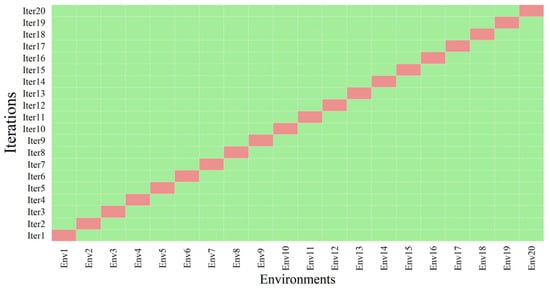
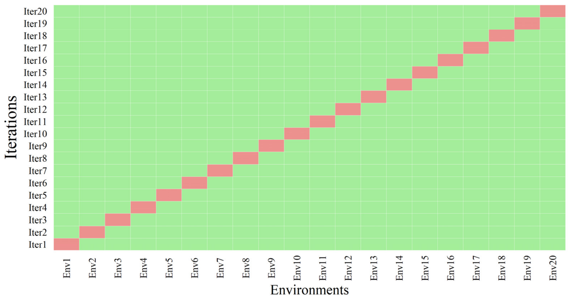
The training process followed a Leave-One-Environment-Out (LOEO) cross-validation scheme to assess the model’s predictive ability on unseen environmental conditions (Figure 1). In each iteration, one environment was held out for validation, while the remaining environments were used to train the model. The number of variables randomly sampled as candidates at each split was set to one (mtry = 1). To guarantee reproducibility, a fixed random seed of 42 was set prior to model fitting. A forest architecture of 500 decision trees was specified to ensure a stable convergence of predictive outcomes. The Random Forest models were implemented using the randomForest R package (version 4.7-1.1) [21].
Figure 1.
Schematic representation of the Leave-One-Environment-Out (LOEO) cross-validation strategy. In each of the I = 20 iterations, one environment is sequestered as the validation set (orange), while the remaining I − 1 environments are utilized for training the Random Forest model (green).
To evaluate the model’s predictive performance, we computed the predictive ability, coefficient of determination (R2), and the Root Mean Squared Error (RMSE). Predictive ability was quantified using the Pearson correlation coefficient (r) between observed and out-of-sample predicted values, that is, . The R2, representing the proportion of phenotypic variance captured by the model, was calculated as
where yi is the observed value for the i-th genotype, is the predicted value for the i-th genotype, and is the overall mean of the observed values.
Finally, the Root Mean Squared Error (RMSE) was determined as
where n represents the total number of observations evaluated across the validation datasets (n = g × e = 180).
2.4. SHAP-Based Local Additive Decomposition of G × E Interactions and Selection Indices
To interpret the complex and non-linear dynamics captured by the RF model, we employed the SHapley Additive exPlanations (SHAP) framework [10]. Rooted in cooperative game theory [12], the Shapley offers a mathematically rigorous method to distribute payoffs fairly among features based on their marginal contributions to model predictions. These values satisfy the fundamental axioms of efficiency (additivity), symmetry, and nullity [10,12]. Specifically, efficiency dictates that the sum of feature contributions plus the baseline value equals the total prediction; symmetry ensures that features with identical contributions receive equal values; and the nullity (dummy) axiom ensures that features with no marginal contribution are assigned a value of zero [22].
In this G × E interaction context, SHAP provides an additive feature attribution method, that decomposes the predicted GY () for the mean of the i-th genotype in the j-th environment into the sum of the effects of GEN and ENV_INDEX. The model prediction can be expressed as
where is the predicted GY by the tree-based model for the mean of each genotype in each environment (), ϕ0 is the overall mean representing the baseline (mean predicted value), and is the Shapley value for the i-th genotype evaluated in the j-th environment (i = 1, 2, …, 9 and j = 1, 2, …, 20). Thus, denotes the Shapley value corresponding to the mean of each combination between the i-th genotype and the j-th environment.
The Shapley value for each gij combination is calculated as follows:
where ϕij(x) is the Shapley value for the i-th genotype in the j-th environment; n is the total number of genotype-by-environment (G × E) combinations (n = 180); N is the set of all evaluated G × E combinations; S represents a subset or coalition that excludes the ij-th combination; the summation encompasses all possible coalitions that can be formed excluding the ij-th combination; f(·) is the characteristic function that assigns a value to each coalition S; and [f(S ∪ {ij}) − f(S)] represents the marginal contribution of the ij-th combination to coalition S. Consequently, each feature (G × E combination) receives a value proportional to its marginal contribution on GY across all possible coalitions.
Given the combinatorial complexity of exact Shapley computation, we estimated the values using the DALEX framework (version 2.5.4) [23], which utilizes Monte Carlo sampling with 25 permutations to approximate the feature contributions efficiently. The mean values for each genotype x environment combination () were used as the input dataset. This procedure allowed us to quantify the localized impact of both genetic and environmental effects on GY, providing a view of the G × E interaction that traditional linear models often obscure.
To facilitate the interpretation of these model outputs for plant breeding applications, we derived three metrics based on the SHAP values: SHAP Effect (SHAPEff), SHAP Stability (SHAPStb) and the SHAP Simultaneous Selection Index (SHAPSSI).
The SHAP Effect quantifies the overall performance of a genotype across all tested environments. It is computed as the mean SHAP value attributed to the i-th genotype across E environments:
where is the Shapley value for the i-th genotype evaluated in the j-th environment, measuring its local marginal contribution to the phenotypic prediction, and E is the total number of evaluated environments (j = 1, 2, …, E). Positive SHAPEff values denote high-performing genotypes with favorable mean phenotypic contribution.
The SHAP Stability is defined as the sample standard deviation of the SHAP values for a given genotype across all evaluated environments, expressed as
where SHAPStb represents the interaction stability index for the i-th genotype across E environments. Lower values of SHAPStb indicate lower sensitivity to environmental variations, signifying higher phenotypic stability.
Finally, the SHAP Simultaneous Selection Index (SHAPSSI), which enables balanced selection between mean yield performance (SHAPEff) and stability (), is defined as
where r_SHAPEff and r_SHAPStb are the rescaled values (0–100) for SHAPEff and SHAPStb (100–0), respectively, and θY and θS represent the relative weights assigned to mean response and stability, set to 60 and 40 in this study, respectively, thereby prioritizing mean performance. Consequently, genotypes exhibiting higher values for SHAPSSI combine high predictive yield performance with robust environmental stability, representing ideal candidates for selection.
To bridge the gap between localized predictions and breeder-oriented selection criteria, individual Shapley values (ϕij), which quantify environmental-specific marginal contributions, are aggregated across all evaluated environments (E). Specifically, the SHAP Effect (SHAPEff) averages these local contributions to capture broad adaptation, while the SHAP Stability (SHAPStb) computes their standard deviation to measure environmental sensitivity. Finally, these aggregated metrics are synthesized into the SHAP Simultaneous Selection Index (SHAPSSI), balancing overall yield potential and non-linear stability into a unified, weighted ranking score for genotype recommendation.
To empirically assess whether the isolated genotype-by-environment interaction profiles exhibit linear or complex non-linear behaviors along the environmental gradient, a SHAP dependence plot was implemented. The continuous environmental index (ENV_INDEX) was specified on the horizontal axis against the genotype-specific Shapley values (SHAPG×E = ϕij, that is, the Shapley value for the i-th genotype evaluated in the j-th environment) on the vertical axis. Non-parametric Locally Estimated Scatterplot Smoothing (LOESS) curves were fitted for each genotype across the ENV_INDEX to visually inspect response curvature, potential non-monotonic trends, and slope changes that signal localized non-linear G × E dynamics.
2.5. Methodological Concordance and Statistical Assessment
Six distinct rankings were established for the evaluated genotypes based on: Grain Yield (GY), AMMI Stability Value (ASV), Simultaneous Selection Index (SSI), SHAP Effect (SHAPEff), SHAP Stability (SHAPStb), and SHAP Simultaneous Selection Index (SHAPSSI). Each genotype was assigned a relative rank ranging from 1 to 9 within each category. For GY, SHAPEff, and SHAPSSI, higher raw values are desirable, so the highest value receives Rank 1. Conversely, for ASV, SSI, and SHAPStb, lower raw values are desirable, so the lowest value receives Rank 1. In all cases, Rank 1 indicates the most preferred genotype. Spearman’s rank correlation coefficient was used to assess the concordance of the relative ranks of genotypes across the different evaluation models, calculated using the following expression:
where is the estimated Spearman’s rank correlation coefficient between rankings A and B; g is the total number of genotypes (g = 9); and di is the difference between the relative ranks of the i-th genotype in rankings A and B. A hypothesis test was performed to assess the significance of the Spearman rank correlation coefficient (H0:ρ = 0; H1:ρ ≠ 0), and the confidence interval for Spearman’s rank correlation was obtained via bootstrap.
All statistical analyses and graphical representations were performed using R software (R-version 4.3.2) [24]. The complete R script used for these analyses is publicly available at https://wevertongomescosta.github.io/nonlinear-ge-interaction-shap/(acessed on 16 October 2026).
3. Results
3.1. Phenotypic Performance Across Environments and Genotypes
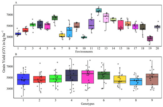
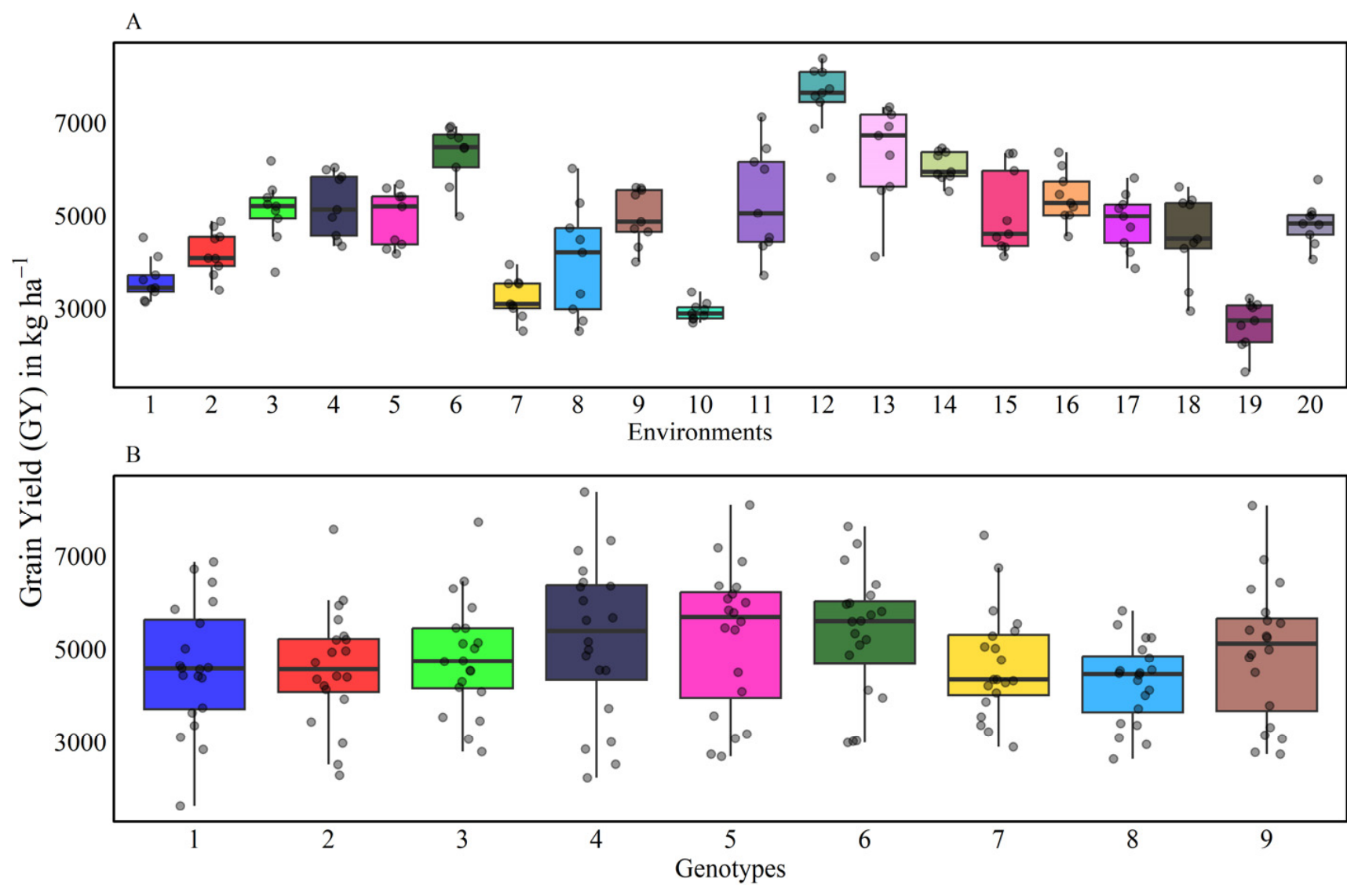
The Grain Yield (GY) (kg ha−1) for the environments and genotypes are presented in Figure 2. The GY across the 20 environments ranged from 2652.00 kg ha−1 (Environment 19) to 7516.00 kg ha−1 (Environment 12). The distributions indicate differences in GY potential across most growing conditions (Figure 2A). Regarding genotypic performance (Figure 2B), the GY means ranged from 4283.00 kg ha−1 (Genotype 8) to 5330.00 kg ha−1 (Genotype 6). The overlapping regions observed among the top-performing materials suggest that Genotype 6 presented a similar GY profile to genotypes 4 (5218.00 kg ha−1) and 5 (5247.00 kg ha−1) (Figure 2B), with all three sustaining average yields superior to the general experimental mean of 4858.13 kg ha−1.
Figure 2.
Phenotypic variability of Grain Yield (GY) across structural factors: (A) distribution of GY across twenty growing environments, and (B) performance and stability of genotypes.
3.2. Machine Learning Model Fitting and Predictive Ability
The Random Forest (RF) model showed high predictive performance under the Leave-One-Environment-Out (LOEO) cross-validation scheme, explaining 85% of the phenotypic variances for GY, with a cross-validation coefficient of determination (R2) of 71.94% and a Root Mean Squared Error (RMSE) of 717.02 kg ha−1. These results provided a reliable basis for the subsequent application of SHAP additive decomposition to study the localized interaction effects.
3.3. Linear and Non-Linear Genotype-by-Environment Decompositions
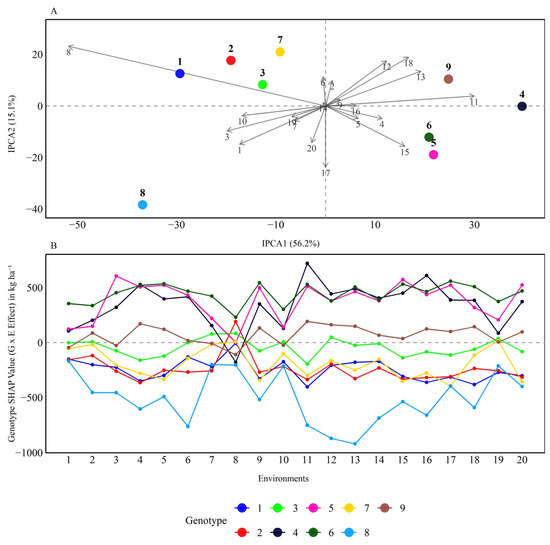
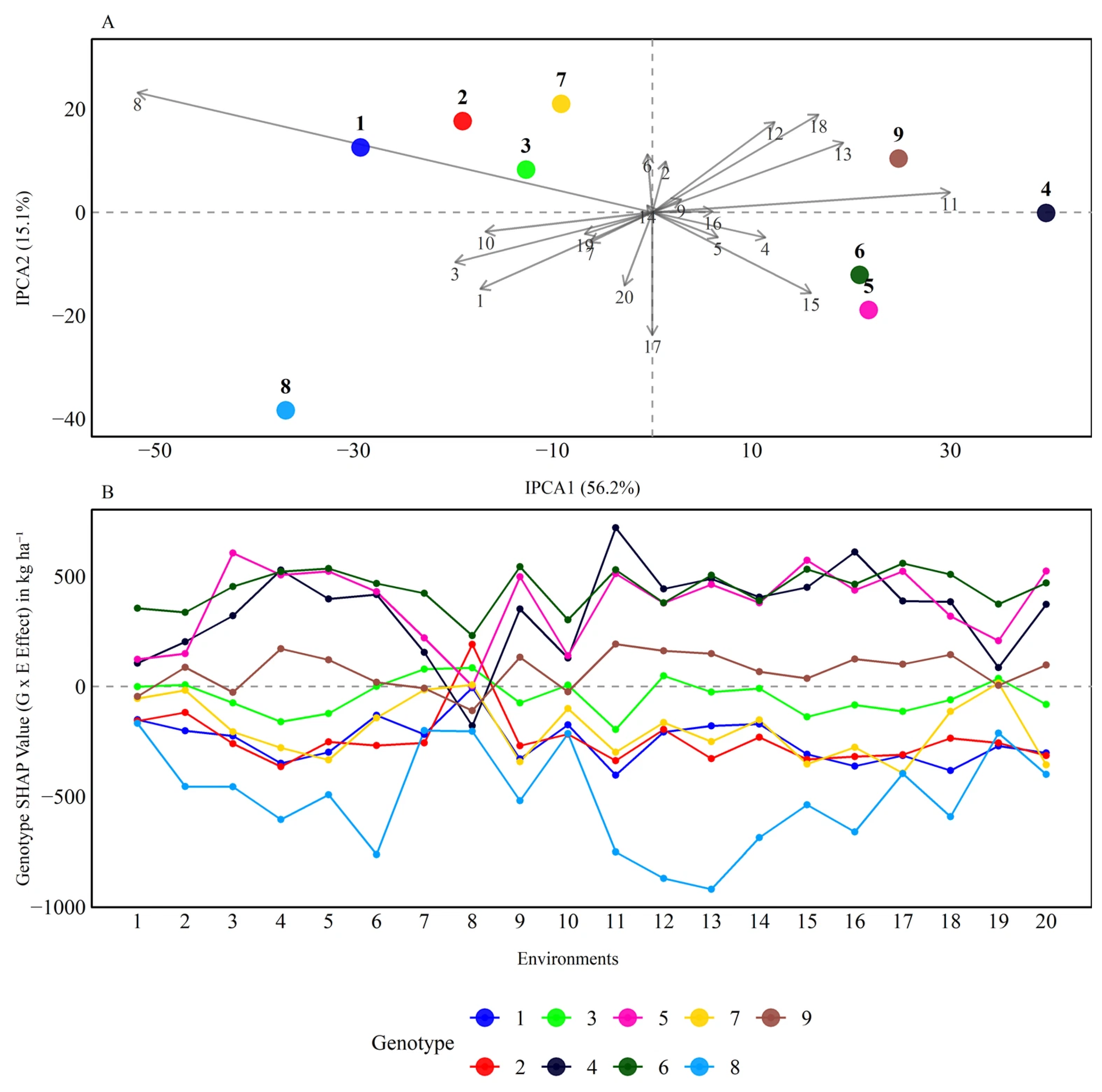
The interaction patterns derived from the AMMI biplot analysis, and the adaptability profiles isolated via SHAP decomposition are concurrently illustrated in Figure 3. The retention of the first two interaction principal component axes (IPCA1 and IPCA2) in the AMMI model was based on capturing a cumulative 71.30% of the total G × E interaction sum of squares. This proportion ensures that the primary bilinear pattern of interaction is retained while minimizing the inclusion of residual noise (Figure 3A). Genotypes 4 and 8, along with environments 8 and 11, positioned farthest from the biplot center, identified them as the major contributors to the G × E interaction. When the interaction is elucidated across environments individually using the SHAP framework (Figure 3B), additional resolution of the complex and non-linear trajectories is achieved, complementing the global view provided by AMMI. Genotypes 4, 5, and 6 presented the highest positive SHAP values across most environments, demonstrating superior adaptability. A convergence between frameworks was identified in Environment 11, where Genotype 4 was positioned far from the biplot origin in the AMMI analysis (Figure 3A), and its maximum positive SHAP interaction effect, exceeding 500 kg ha−1 (Figure 3B). In addition, Genotype 8 presented negative contributions throughout the evaluation sites, achieving its worst performance in Environment 13, where its negative interaction effect dropped below −500 kg ha−1. The SHAP framework also successfully tracked localized response shifts that are typically smoothed over by global linear biplots. For instance, in Environment 8, a ranking inversion occurred where Genotypes 4 and 6 suffered severe performance drops, while Genotypes 1 and 2, which generally underperformed, exhibited sharp positive values (Figure 3B).
Figure 3.
Linear and non-linear genotype-by-environment (G × E) interaction structures for maize Grain Yield: (A) traditional AMMI biplot showing the projection of genotypes and environments on the first two interaction principal components (IPCA1 and IPCA2), and (B) non-linear adaptability profiles isolated via SHAP decomposition tracking localized genotype contributions across the 20 environments.
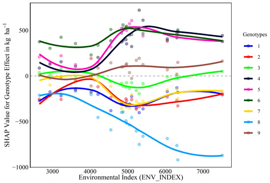
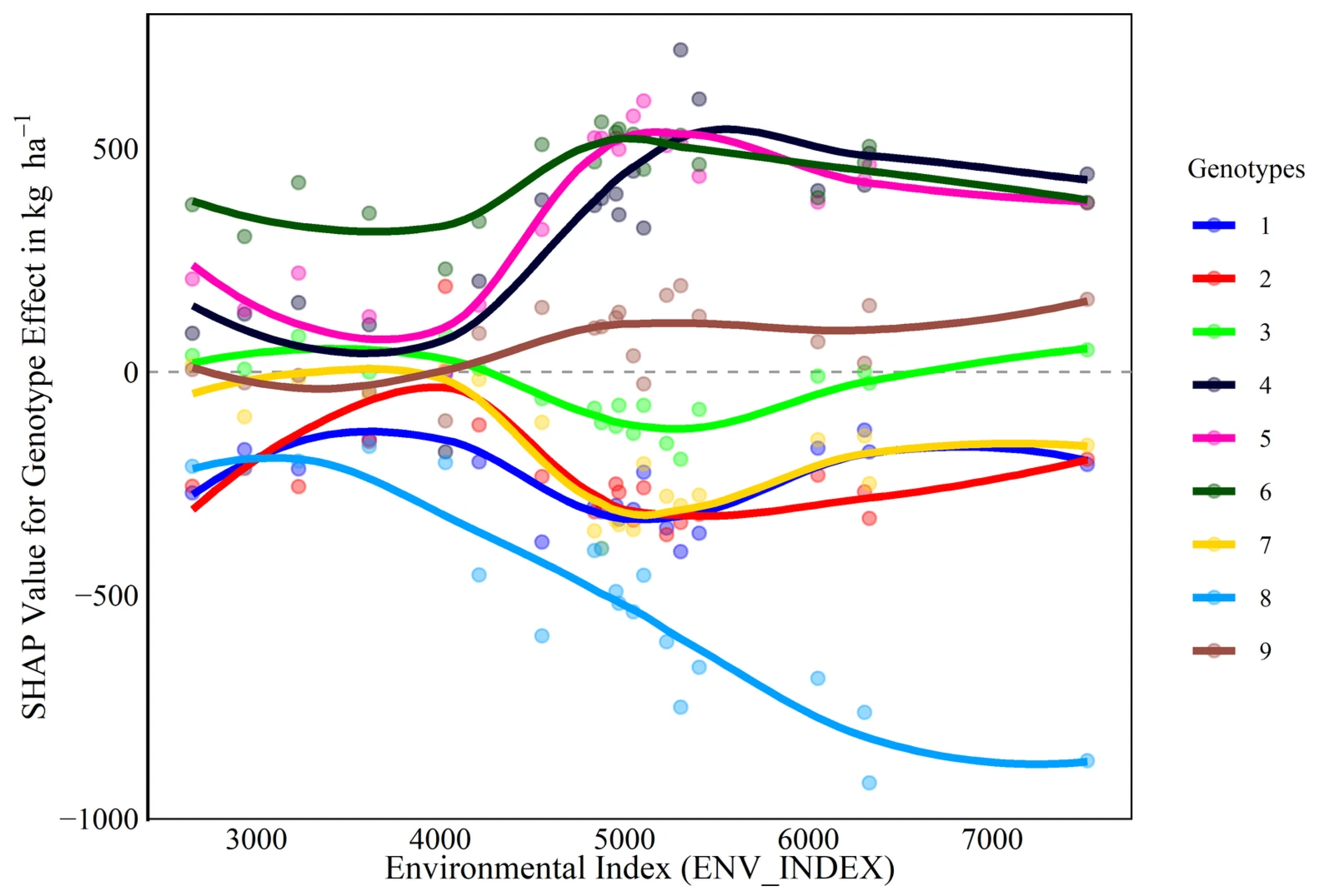
Beyond evaluating discrete environmental sites, the continuity of the G × E interaction was investigated via the SHAP dependence plot fitted with LOESS non-parametric smooth curves along the continuous environmental gradient (ENV_INDEX) (Figure 4). The observed trajectories clearly departed from straight linear responses, exhibiting curvatures, inflections, and non-monotonic fluctuations across contrasting yield potentials. Furthermore, multiple curve intersections (crossovers) were identified along the ENV_INDEX, providing evidence that the underlying G × E interaction dynamics in this dataset are inherently non-linear and cannot be fully captured by traditional linear or bilinear assumptions.
Figure 4.
SHAP dependence plot depicting genotype-specific marginal interaction contributions (SHAPGEN) across the environmental index (ENV_INDEX). Solid lines represent non-parametric LOESS smooth curves fitted for each genotype to illustrate non-linear G × E response dynamics and crossover interactions.
3.4. Genotype Rank Dynamics Across Linear and Non-Linear Selection Frameworks
Regarding the per se performance, the GY ranking ranged from Genotype 6 (rank 1, most productive) to Genotype 8 (rank 9, least productive; Table 1). The top two yielding materials, Genotypes 6 and 5, exhibited intermediate to low linear stability scores, ranking 4th and 5th under the ASV framework, respectively, which makes them less desirable from a stability point of view (Table 1). Conversely, when evaluated under the complex and non-linear SHAP stability framework (SHAP Stability), Genotype 6 maintained a superior position, ranking 3rd, whereas Genotype 4 dropped to the 8th position. This contrast highlights that, although both materials exhibit high phenotypic yield potential, they possess distinct profiles, with Genotype 6 showing a higher non-linear stability than Genotype 4 (Table 1).
Table 1.
Genotype rank transitions across phenotypic performance, parametric linear indices, and non-linear SHAP frameworks. For each genotype, values are presented as raw estimate (rank), where the value corresponds to the genotype’s actual estimate for that criterion and the number in parentheses indicates its ordinal position (1 = best, 9 = worst) among the nine genotypes. The selection criteria are: Grain Yield (GY, kg ha−1), AMMI stability value (ASV), simultaneous selection index (SSI), and the proposed machine learning metrics (SHAPEff is SHAP Effect, SHAPStb is SHAP Stability, and SHAPSSI is SHAP Simultaneous Selection Index).
When the simultaneous selection frameworks are compared, the conventional linear index (SSI) and the novel non-linear Machine Learning approach (SHAP SSI) revealed highly complementary selection patterns (Table 1). A convergence between the two frameworks was observed for the top-performing material. Genotype 6 was consistently ranked first under the per se GY, the conventional SSI, and the integrated SHAP SSI. This alignment confirms that its GY superiority and high non-linear stability converge perfectly when capturing complex interaction dynamics. In contrast, rank changes were observed for intermediate and other high-yielding materials when shifting from linear to non-linear selection models (Table 1). Genotype 5, which achieved the second highest per se GY and was positioned 3rd under the conventional linear SSI, exhibited a decline to the 7th position under the isolated SHAP Stability framework. Conversely, Genotype 4 showed an inverse rank trajectory which was penalized by the linear AMMI stability index (rank = 9) and dropped to the 7th position under the conventional SSI, it displayed a higher non-linear main effect under the SHAP Effect framework (rank = 3), which ultimately repositioned it at the 5th place under the integrated SHAP SSI (Table 1).
Finally, at the lower end of the selection spectrum, a systematic consensus was maintained. Specifically, Genotype 8 consistently occupied the worst possible positions across almost all frameworks (rank 8 or 9), including a systematic lowest placement (rank 9) in both the conventional SSI and the proposed SHAP SSI, fully validating its poor agronomic performance and lack of systemic stability (Table 1).
3.5. Rank Correlation Analysis Among Phenotypic Performance and Stability Metrics
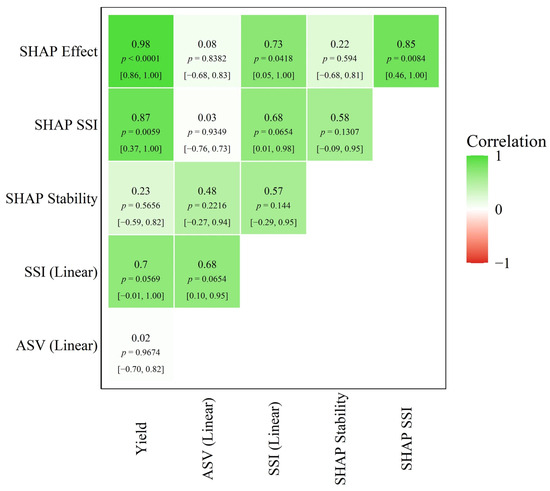
The Spearman rank correlation coefficients () among per se performance (GY), linear stability indices (ASV and SSI), and the non-linear ML-based framework metrics (SHAPEff, SHAPStb and SHAPSSI) are presented in Figure 5. The magnitude and direction of the correlation coefficients reveal how effectively each framework aligns with GY and tracks genotype classification patterns.
Figure 5.
Spearman rank correlation matrix across phenotypic yield and stability frameworks. The upper-triangular matrix displays the Spearman correlation coefficients () among Grain Yield (GY), AMMI Stability Value (ASV), Simultaneous Selection Index (SSI), and the proposed Machine Learning metrics (SHAPEff, SHAPStb and SHAPSSI). Values closer to 1 or −1 indicate stronger positive or negative rank agreement, respectively. For each cell, the middle line reports the two-sided p-value for the null hypothesis of no rank correlation, and the bottom line reports the 95% bootstrap confidence interval (CI).
Both stability indices, the linear ASV ( with GY, p = 0.9674) and the non-linear SHAP Stability ( with GY, p = 0.5656), showed low correlations with GY, confirming that stability and productivity represent independent dimensions of genotype performance (Figure 5). The proposed non-linear SHAPSSI exhibited the high correlation with GY (, p = 0.0059), outperforming the classical linear SSI (, p = 0.0569). This indicates that while the SHAPSSI successfully integrates non-linear stability, it remains highly effective at selecting for top-yielding genotypes. This behavior is further supported by the near-perfect correlation between GY and the SHAP Effect (, p < 0.0001), demonstrating that the SHAP decomposition captures the genetic main effects on yield (Figure 5).
4. Discussion
In this study, we performed a tree-based Machine Learning (ML) framework under a predictive approach and proposed SHAP-based measures (SHAPEff, SHAPStb and SHAPSSI) aiming to perform jointly inference on yield stability and performance. Using nine genotypes evaluated in 20 environments in a randomized block design with four replicates, the results were compared to those derived from the traditional frequentist linear framework AMMI (ASV and SSI). Although Figure 2B is descriptive, the apparent differences among genotypes (including the superior performance of genotypes 4, 5, and 6) are statistically supported by [17], which reports 90% highest posterior density (HPD) intervals for the same dataset.
Evaluated via a Leave-One-Environment-Out (LOEO) cross-validation framework, the Random Forest (RF) demonstrated robust predictive performance, yielding a high predictive ability of 0.85, a coefficient of determination (R2) of 71.94%, and a root mean squared error (RMSE) of 717.02 kg ha−1. The high predictive ability demonstrates that the ML algorithm captured biological signals [25] validating the subsequent application of SHAP additive decomposition to study the localized interaction effects. This includes complex, non-linear genotype-by-environment (G × E) interactions that typically can inflate the residual errors of traditional bilinear models [26].
It is worth noting that using the environmental mean yield (ENV_INDEX) as a continuous covariate introduces a degree of circularity, since the response variable (GY) is utilized to construct its own predictor. In predictive modeling, such trait-derived covariates can inflate goodness-of-fit metrics (e.g., R2 and RMSE). Despite that, in our study, employing ENV_INDEX allowed us to provide a fair benchmark between SHAP-interpreted machine learning models and classical bilinear approaches (AMMI and GGE), which depend on environment main-effect averages. To avoid this circularity and better isolate physiological stress, thereby enhancing dynamic yield prediction across unobserved target populations of environments, future research should prioritize replacing or supplementing this aggregate index with independent environmental covariates, such as daily meteorological and edaphic variables.
The adoption of tree-based and ML algorithms, such as RF and Bagging and Boosting, to model and predict G × E interactions has gained significant importance in the recent plant breeding literature. This trend is well-illustrated by recent applications optimizing genomic prediction in multi-environment maize trials and mapping non-linear genetic interactions such as epistasis across variable environments [27].
The SHAP framework allowed to elucidate localized response shifts and micro-environmental dynamics that are not directly represented in linear and bilinear biplots (Figure 3). To directly test whether the G × E interaction follows a linear behavior along the environmental gradient, a SHAP dependence plot was constructed using LOESS smoothing across the continuous environmental index (ENV_INDEX) (Figure 4). The resulting response curves clearly departed from straight lines, exhibiting pronounced curvatures, inflections, and slope changes. This empirical pattern confirms that the G × E interaction in this germplasm network is governed by non-linear dynamics. Traditional biometric models, such as AMMI and GGE, rely on singular value decomposition (SVD) to capture the primary axes of variation; specifically, a mathematical constraint that inherently prioritizes global variance maximization at the expense of environment-specific, non-linear anomalies. This limitation becomes highly evident when analyzing localized interaction profiles within specific target environments. For instance, in Environment 8, a severe crossover G × E interaction and ranking inversion occurred. Specifically, Genotypes 4 and 6, which sustained superior genetic main effects across the macro-environmental network, suffered pronounced localized performance drops. Concurrently, Genotypes 1 and 2, which generally underperformed under broad conditions, exhibited sharp positive SHAP values within this specific trial (Figure 3B).
In classical biplot representations, such localized crossovers are frequently obscured if the unique interaction vector of a single environment does not align with the first two principal component axes. Thus, the proposed method provides an additive local decomposition for every unique G × E combination avoiding the dilution of these specific adaptability trends. For plant breeders, uncovering these localized changes is paramount for identifying specific environmental sites and deciphering the underlying physiological or agronomic mechanisms driving conditional resilience or susceptibility. This Explainable Artificial Intelligence (XAI) framework utilizes non-linear SHAP decomposition to effectively model localized ranking inversions, thereby avoiding specific G × E signals from being lost within the residual error matrix. XAI algorithms have emerged to open machine learning ‘black boxes’ by identifying the key drivers of predictive outcomes [28,29,30]. In plant breeding, bridging high predictive accuracy with biological interpretability is crucial for unraveling complex trait architecture, resolving marker effects, and estimating heritability to guide selection decisions [9].
The divergence between the conventional AMMI stability value (ASV) and the non-linear SHAP framework underscores the limitations of relying on linear assumptions to evaluate high-yielding germplasm under complex G × E interactions. As illustrated by the LOESS-fitted SHAP dependence curves (Figure 4), the trajectory of genotype-specific effects along ENV_INDEX varies substantially: while Genotype 6 demonstrates a sustained, non-linear resilience across contrasting environments, Genotype 4 exhibits sharp, non-monotonic fluctuations. While traditional biplots confounded the stability profiles of Genotypes 6 and 4, the SHAP framework successfully decoupled them, revealing that Genotype 6 possesses robust non-linear resilience whereas Genotype 4 is highly sensitive to non-linear environmental fluctuations that linear models smooth over.
Regarding the ranking dynamics across the linear and non-linear selection frameworks, the most productive genotypes were generally not identified as the most stable materials (Figure 3). This divergence reflects genotype-specific environmental sensitivity, which may lead to environment-dependent performance, changes in genotype ranking, and specific rather than broad adaptation [31,32]. Consequently, employing simultaneous selection indices that integrate both yield and stability represents the most robust breeding strategy to optimize genetic gains [33]. Both the conventional selection index (SSI) and the novel SHAP SSI exhibited concordance in recommending Genotypes 5 and 6 as the top three selections. Discrepancies within the top three ranks were observed for Genotypes 9 (G9) and 3 (G3). Genotype 9, which ranked fifth under the linear SSI, rose to second place under the integrated non-linear SHAPSSI. It is worth noting that the SHAPSSI, analogous to the WAASBY index proposed by [33], is a simultaneous selection tool that combines genotype stability and mean performance based on user-defined weight scenarios.
Although selection indices are useful when analyzing multiple genotypes simultaneously, they can mask key performance details. The non-linear adaptability profiles obtained via SHAP decomposition (Figure 3) and continuous dependency curves (Figure 4) reveal the underlying drivers of complex interactions and pinpoint genotype performance across specific environments. For instance, using this figure as an auxiliary tool, it is clear that Genotype 9 (favored by the SHAPSSI) exhibits a superior and more stable response profile than Genotype 3 (favored by the linear SSI). Additionally, the SHAP curves reveal specific adaptabilities that are completely omitted by the biplot, such as the localized high performance of Genotype 5 in specific environmental subsets. Specifically, while the bilinear biplot suggests poor adaptation for Genotype 5 across several environments, as indicated by the angles between the genotype and environmental vectors, the non-linear SHAP profiles demonstrate a much more favorable performance in several of these settings.
The absence of linear relationship between crop productivity and stability was confirmed by the weak rank correlations of grain yield with both the linear ASV (, p = 0.9674) and non-linear SHAP Stability (, p = 0.5656), highlighting the importance of simultaneous selection frameworks (Table 1). In this context, the proposed non-linear SHAP SSI showed a stronger rank correlation with yield ( p = 0.0059) than the traditional linear SSI ( p = 0.0569), suggesting complementary selection efficiency. A near-perfect correlation was observed between grain yield and the SHAP Effect (, p < 0.0001), validating the model’s biological accuracy (Figure 5). The moderate correlation between the two indices (linear SSI and SHAP SSI; , p = 0.0654) explains rank discrepancies, such as the SHAP SSI favoring Genotype 9 over Genotype 3, which exhibited negative marginal contributions across almost all environments despite its high linear SSI ranking (Figure 3).
Altogether, these results reinforce the importance of the ML predictive approach combined with the SHAP framework, as an auxiliary tool, to infer about the potential of the candidates (genotypes or environments) that are responsible for the G × E interaction or to select or recommend these genotypes based on the SHAPSSI. Specifically, the linear and bilinear approaches do not capture complex, non-linear interactions (which are often smoothed over or relegated to the residual error matrix), and for the biplot projection, specific localized adaptabilities can be easily masked or confounded due to the mathematical constraints of low-dimensional variance maximization.
In practice, the predictive and interpretive capabilities of this non-linear SHAP-based machine learning approach have interesting implications for breeding research. By providing more informative statistical tool at both global and local levels, this framework can help the breeders to make better decisions about genotype selection and targeted recommendation. This can ultimately lead to the development of more stable, resilient, and high-yielding varieties across diverse and fluctuating environmental conditions.
It is important to emphasize that traditional bilinear approaches, such as AMMI, and machine learning frameworks integrated with SHAP serve complementary, rather than mutually exclusive, roles in G × E analysis. By design, AMMI provides a parsimonious linear/bilinear decomposition of main effects and interaction components, making it an intuitive tool for general adaptability and stability classification (e.g., via ASV and SSI). Conversely, AMMI is not mathematically structured to detect complex, non-linear relationships. Tree-based machine learning models combined with SHAP complement this classical baseline by capturing local, non-linear patterns and threshold effects across continuous environmental gradients that might otherwise remain obscured in bilinear representations.
The validity of the proposed SHAP-based framework inherently relies on the predictive performance of the trained machine learning model, making robust cross-validation essential to guarantee reliable biological interpretations. Although computational costs may increase when scaling the analysis to larger datasets, this constraint can be effectively managed. For large-scale breeding programs, linear or sampled approximations of SHAP (such as KernelSHAP or optimized path-dependent variations in TreeSHAP) can be readily deployed to enable computationally efficient and highly scalable model interpretations.
Finally, replacing or complementing this aggregate index with independent, high-resolution enviromic covariates (such as daily meteorological and edaphic variables) represents a natural next frontier to eliminate circularity. Future research leveraging multidimensional environmental predictors will bypass trait-derived dependencies and fully unlock SHAP’s capacity to pinpoint specific physiological stress thresholds, ultimately enabling dynamic yield predictions across unsampled target populations of environments.
5. Conclusions
The proposed approach, leveraging Machine Learning algorithms integrated with local additive SHAP decomposition, enabled the evaluation of complex, non-linear genotype-by-environment (G × E) interactions, offering breeders a complementary perspective for the selection of stable and responsive genotypes alongside traditional linear models. Furthermore, comparison with traditional AMMI analysis, via stability rankings and adaptability profiles, indicates that this methodology can serve as a complementary tool for decision-making in plant breeding, as it provides additional resolution of G × E interactions across the evaluated environments.
Author Contributions
Conceptualization, M.N., N.M.E.P.d.L.d.C. and A.C.C.N.; methodology, M.N., A.C.C.N., N.M.E.P.d.L.d.C., W.G.d.C., W.A.L.P. and D.J.; software, M.N., A.C.C.N., N.M.E.P.d.L.d.C. and W.G.d.C.; validation, M.N., A.C.C.N., W.G.d.C. and D.J.; formal analysis, M.N., A.C.C.N., N.M.E.P.d.L.d.C. and W.G.d.C.; investigation, M.N., A.C.C.N., N.M.E.P.d.L.d.C., W.G.d.C., W.A.L.P. and D.J.; resources, M.N., A.C.C.N. and D.J.; data curation, M.N.; writing—original draft preparation, M.N. and N.M.E.P.d.L.d.C.; writing—review and editing, M.N., A.C.C.N., N.M.E.P.d.L.d.C., W.G.d.C., W.A.L.P. and D.J.; visualization, M.N., A.C.C.N., N.M.E.P.d.L.d.C., W.G.d.C., W.A.L.P. and D.J.; supervision, M.N.; project administration, M.N. and A.C.C.N. All authors have read and agreed to the published version of the manuscript.
Funding
We would like to thank the Brazilian Federal Agency for Support and Evaluation of Graduate Education (CAPES), Finance Code 001, and the National Council of Scientific and Technological Development (CNPq, 408833/2023-8). M.N. and A.C.C.N. are supported by scientific productivity grants (310755/2023-9 and 311841/2025-2) from Brazilian Council for Scientific and Technological Development (CNPq).
Institutional Review Board Statement
Not applicable.
Data Availability Statement
The data presented in this study are openly available in GITHUB at https://wevertongomescosta.github.io/nonlinear-ge-interaction-shap/(acessed on 16 October 2026).
Acknowledgments
We would like to thank the Federal University of Viçosa. Federal University of Tocantins and the University of Florida for providing the necessary knowledge to develop this work.
Conflicts of Interest
The authors declare no conflicts of interest.
References
- Jędzura, S.; Bocianowski, J.; Matysik, P. The AMMI model application is used to analyze the genotype–environmental interaction of spring wheat grain yield for breeding program purposes. Cereal Res. Commun. 2023, 51, 197–205. [Google Scholar] [CrossRef] [Scilit]
- Zobel, R.W.; Wright, M.J.; Gauch, H.G., Jr. Statistical analysis of a yield trial. Agron. J. 1988, 80, 388–393. [Google Scholar] [CrossRef] [Scilit]
- Gauch, H.G.; Piepho, H.-P.; Annicchiarico, P. Statistical analysis of yield trials by AMMI and GGE: Further considerations. Crop Sci. 2008, 48, 866–889. [Google Scholar] [CrossRef] [Scilit]
- Kempton, R.A. The use of biplots in interpreting variety by environment interactions. J. Agric. Sci. 1984, 103, 123–135. [Google Scholar] [CrossRef] [Scilit]
- Gauch, H.G.; Zobel, R.W. Imputing missing yield trial data. Theor. Appl. Genet. 1990, 79, 753–761. [Google Scholar] [CrossRef] [Scilit] [PubMed]
- van Eeuwijk, F.A.; Bustos-Korts, D.V.; Malosetti, M. What should students in plant breeding know about the statistical aspects of genotype × environment interactions? Crop Sci. 2016, 56, 2119–2140. [Google Scholar] [CrossRef] [Scilit]
- Fritsche-Neto, R.; Resende, R.T.; Olivoto, T.; Garcia-Abadillo, J.; Nascimento, M.; Bahia, M.A.M.; Jarquin, D.; Vieira, R.A. Prediction-based breeding: Modern tools to optimize and reshape programs. Crop Sci. 2025, 65, e70175. [Google Scholar] [CrossRef] [Scilit]
- Montesinos-López, O.A.; Montesinos-López, A.; Pérez-Rodríguez, P.; Barrón-López, J.A.; Martini, J.W.R.; Fajardo-Flores, S.B.; Gaytan-Lugo, L.S.; Santana-Mancilla, P.C.; Crossa, J. A review of deep learning applications in plant breeding. Theor. Appl. Genet. 2021, 134, 1613–1630. [Google Scholar] [CrossRef] [Scilit] [PubMed]
- Sousa, I.C.; Nascimento, M.; Sant’Anna, I.C.; Caixeta, E.T.; Azevedo, C.F.; Cruz, C.D.; Silva, F.L.; Alkimim, E.R.; Nascimento, A.C.C.; Serão, N.V.L. Marker effects and heritability estimates using additive-dominance genomic architectures via artificial neural networks in Coffea canephora. PLoS ONE 2022, 17, e0262055. [Google Scholar] [CrossRef] [Scilit] [PubMed]
- Lundberg, S.M.; Lee, S.-I. A unified approach to interpreting model predictions. In Proceedings of the 31st International Conference on Neural Information Processing Systems, Long Beach, CA, USA, 4–9 December 2017. [Google Scholar] [CrossRef] [Scilit]
- Qin, L.; Zhu, Y.; Liu, S.; Zhang, X.; Zhao, Y. The Shapley Value in Data Science: Advances in Computation, Extensions, and Applications. Mathematics 2025, 13, 377. [Google Scholar] [CrossRef] [Scilit]
- Shapley, L.S. A value for n-person games. In Contributions to the Theory of Games II, 1st ed.; Kuhn, H.W., Tucker, A.W., Eds.; Princeton University Press: Princeton, NJ, USA, 1953; pp. 307–317. [Google Scholar] [CrossRef] [Scilit]
- Cornelius, P.L.; Seyedsadr, M.; Crossa, J. Using the shifted multiplicative model to search for “separability” in crop cultivar trials. Theor. Appl. Genet. 1992, 84, 161–172. [Google Scholar] [CrossRef] [Scilit] [PubMed]
- Nascimento, A.C.C.; Nascimento, M.; Sagae, V.S.; Destro, V.; Nardino, M.; Olivoto, T.; Jarquín, D. Bayesian AMMI-based indexes for genotype selection: Integrating novel stability measures for enhanced G × E inference. Crop Sci. 2025, 65, e70140. [Google Scholar] [CrossRef] [Scilit]
- Purchase, J.L.; Hatting, H.; van Deventer, C.S. Genotype × environment interaction of winter wheat (Triticum aestivum L.) in South Africa: II. Stability analysis of yield performance. S. Afr. J. Plant Soil 2000, 17, 101–107. [Google Scholar] [CrossRef] [Scilit]
- Du, Y.-L.; Xi, Y.; Cui, T.; Anten, N.P.R.; Weiner, J.; Li, X.; Turner, N.C.; Zhao, Y.-M.; Li, F.-M. Yield components, reproductive allometry and the tradeoff between grain yield and yield stability in dryland spring wheat. Field Crops Res. 2020, 257, 107930. [Google Scholar] [CrossRef] [Scilit]
- Farshadfar, E. Incorporation of AMMI stability value and grain yield in a single non-parametric index (GSI) in bread wheat. Pak. J. Biol. Sci. 2008, 11, 1791–1796. [Google Scholar] [CrossRef] [Scilit] [PubMed]
- Ho, T.K. Random decision forests. In Proceedings of the 3rd International Conference on Document Analysis and Recognition, Montreal, QC, Canada, 14–16 August 1995. [Google Scholar] [CrossRef] [Scilit]
- Breiman, L.; Friedman, J.H.; Olshen, R.A.; Stone, C.J. Classification and Regression Trees, 1st ed.; Chapman and Hall/CRC: New York, NY, USA, 1984; p. 368. [Google Scholar] [CrossRef] [Scilit]
- Hastie, T.; Tibshirani, R.; Friedman, J. The Elements of Statistical Learning, 2nd ed.; Springer: New York, NY, USA, 2009; p. 745. [Google Scholar] [CrossRef]
- Liaw, A.; Wiener, M. Classification and Regression by randomForest. R News 2002, 2, 18–22. [Google Scholar] [CrossRef] [Scilit]
- Li, M.; Sun, H.; Huang, Y.; Chen, H. Shapley value: From cooperative game to explainable artificial intelligence. Auton. Intell. Syst. 2024, 4, 2. [Google Scholar] [CrossRef] [Scilit]
- Biecek, P. DALEX: Explainers for Complex Predictive Models in R. J. Mach. Learn. Res. 2018, 19, 1–5. [Google Scholar]
- R Core Team. R: A Language and Environment for Statistical Computing, R Version 4.3.2; R Foundation for Statistical Computing: Vienna, Austria, 2023. Available online: https://www.R-project.org/ (accessed on 28 July 2026).
- Howard, R.; Carriquiry, A.L.; Beavis, W.D. Parametric and nonparametric statistical methods for genomic selection of traits with additive and epistatic genetic architectures. Genes Genomes Genet. 2014, 4, 1027–1046. [Google Scholar] [CrossRef] [Scilit] [PubMed]
- Gauch, H.G., Jr. A simple protocol for AMMI analysis of yield trials. Crop Sci. 2013, 53, 1860–1869. [Google Scholar] [CrossRef] [Scilit]
- Costa, W.G.; Celeri, M.O.; Barbosa, I.P.; Silva, G.N.; Azevedo, C.F.; Borém, A.; Nascimento, M.; Cruz, C.D. Genomic prediction through machine learning and neural networks for traits with epistasis. Comput. Struct. Biotechnol. J. 2022, 20, 5490–5499. [Google Scholar] [CrossRef] [Scilit] [PubMed]
- Cilli, R.; Elia, M.; D’Este, M.; Giannico, V.; Amoroso, N.; Lombardi, A.; Pantaleo, E.; Monaco, A.; Sanesi, G.; Tangaro, S.; et al. Explainable artificial intelligence (XAI) detects wildfire occurrence in the Mediterranean countries of Southern Europe. Sci. Rep. 2022, 12, 16349. [Google Scholar] [CrossRef] [Scilit] [PubMed]
- Mostafa, S.; Mondal, D.; Panjvani, K.; Kochian, L.; Stavness, I. Explainable deep learning in plant phenotyping. Front. Artif. Intell. 2023, 6, 1203546. [Google Scholar] [CrossRef] [Scilit] [PubMed]
- Novielli, P.; Romano, D.; Pavan, S.; Losciale, P.; Stellacci, A.M.; Diacono, D.; Bellotti, R.; Tangaro, S. Explainable artificial intelligence for genotype-to-phenotype prediction in plant breeding: A case study with a dataset from an almond germplasm collection. Front. Plant Sci. 2024, 15, 1434229. [Google Scholar] [CrossRef] [Scilit] [PubMed]
- Sabir, K.; Rose, T.; Wittkop, B.; Stahl, A.; Snowdon, R.J.; Ballvora, A.; Friedt, W.; Kage, H.; Léon, J.; Ordon, F.; et al. Stage-specific genotype-by-environment interactions determine yield components in wheat. Nat. Plants 2023, 9, 1688–1696. [Google Scholar] [CrossRef] [Scilit] [PubMed]
- Mbe, J.O.; Dzidzienyo, D.; Abah, S.P.; Njoku, D.N.; Aghogho, C.I.; Onyeka, J.; Tongoona, P.; Egesi, C. Genotype by environment interaction effect and fresh root yield stability of cassava genotypes under contrasting nitrogen regimes. Sci. Rep. 2024, 14, 20709. [Google Scholar] [CrossRef] [Scilit] [PubMed]
- Olivoto, T.; Lúcio, A.D.C.; Silva, J.A.G.; Sari, B.G.; Diel, M.I. Mean performance and stability in multi-environment trials II: Selection based on multiple traits. Agron. J. 2019, 111, 2961–2969. [Google Scholar] [CrossRef] [Scilit]

Disclaimer/Publisher’s Note: The statements, opinions and data contained in all publications are solely those of the individual author(s) and contributor(s) and not of MDPI and/or the editor(s). MDPI and/or the editor(s) disclaim responsibility for any injury to people or property resulting from any ideas, methods, instructions or products referred to in the content. |
© 2026 by the authors. Licensee MDPI, Basel, Switzerland. This article is an open access article distributed under the terms and conditions of the Creative Commons Attribution (CC BY) license.