


Abstract
Compound flash drought–heatwave extremes (FDHW) expose vegetation to rapid water and heat stress, but regional assessments often conflate event detection with vegetation response and rarely resolve delayed canopy trajectories. We quantified FDHW across China’s Northeast Black Soil Region during the 1995–2024 growing seasons using ERA5-Land soil-moisture and temperature thresholds, applied a spatiotemporal graph neural network to regularize threshold-derived event masks, and reserved AVHRR NDVI for independent post-event impact assessment. Flash drought and FDHW frequencies exhibited strong interannual variability rather than a significant monotonic trend. FDHW occurrence increased from 3.8 to 4.8 d per growing season between 1995–2005 and 2016–2024, but the Theil–Sen trend was near zero (0.05 d per decade). Land–atmosphere composites indicate progressive soil-moisture depletion before FDHW occurrence and a transition from latent to sensible heat release roughly three days before maximum temperature anomalies. NDVI composites revealed a delayed greenness response: anomalies were negative through the first two post-event weeks, reached their minimum approximately one week after the reference FDHW grid-day, and then partially recovered during days 16–30. Mean NDVI suppression was modest (short-term −0.009; long-term −0.006), but persistent negative anomalies remained in 12.1% of southern cropland-dominant trajectories and 10.7% of northern forest–crop ecotone trajectories. These results show that FDHW impacts in the NBSR are expressed less as a steady rise in event frequency than as delayed and spatially heterogeneous vegetation stress, highlighting the need for post-event monitoring windows and cross-sensor validation to support agricultural risk assessment and adaptation planning.
1. Introduction
The Northeast Black Soil Region (NBSR) of China, spanning Heilongjiang, Jilin, and Liaoning provinces and eastern Inner Mongolia, is one of the world’s four major black soil zones [1]. Its fertile Mollisols and Chernozems underpin intensive maize and soybean production central to national food security [2]. The region sits in a climatically sensitive mid-latitude belt where warming has outpaced the global average [3], and where predominantly rainfed cropland, locally irrigated or otherwise water-managed cropland, and natural vegetation are increasingly exposed to extreme weather, particularly drought and heat [4,5]. Predicting ecosystem vulnerability and guiding adaptation in this region depends on understanding how vegetation responds when drought and heat co-occur.
Flash drought is particularly relevant in the NBSR because it develops too quickly for many agricultural management responses. Unlike conventional drought, which develops over months to seasons, flash drought is defined by the rapid intensification of soil moisture deficit over days to weeks, frequently accompanied by elevated temperatures and high vapor pressure deficit [6,7]. Rapid onset leaves little time for physiological or management adjustment; stomatal closure and photosynthetic downregulation can occur before crops have developed deeper roots or entered less sensitive phenological stages, and observational evidence indicates that flash drought frequency has increased across many mid-latitude regions as the climate warms [5,8]. Flash droughts often coincide with heatwaves, forming compound drought–heatwave events (FDHW) whose combined water and heat stress can be more severe than either hazard alone [9,10]. Global analyses show that compound dry-hot extremes have intensified, particularly in transitional climate zones where soil moisture often lies near the transition between energy-limited and water-limited evapotranspiration [11,12].
The physiological pathways through which combined drought and heat stress affect vegetation have been documented at leaf and canopy scales. Soil moisture deficit drives stomatal closure, reducing latent heat flux and elevating canopy temperature [13], while high temperatures directly impair Rubisco activity and photosynthetic electron transport. These mechanisms are well established at leaf and canopy scales, but their regional expression remains harder to measure. Threshold-based FDHW detection can break rapidly evolving events into fragmented patches, which propagates into noisy estimates of affected area and vegetation-index anomalies. Impact attribution is further complicated when vegetation indices are used both to identify drought and to measure its consequences: a decline in greenness may become part of the event definition and then be counted again as the event impact. The timing of the vegetation response adds a further complication: if canopy greenness responds several days after meteorological onset, NDVI measured during the event may miss the main response, while later measurements may already reflect recovery or additional stress.
Satellite-based studies have documented spatially heterogeneous vegetation responses to flash drought and compound extremes across Northeast China [14,15], and a technical review shows that optical vegetation indices remain central to ecosystem-stress monitoring while requiring careful attention to sensor, atmospheric, and index-specific limitations [16]. Recent work has advanced deep learning frameworks for detecting compound drought–heatwave events from both historical and future climate scenarios [17]. Quantitative comparison of vegetation recovery trajectories across cropland and semi-natural vegetation following compound events is still lacking, as is work examining how the spatial coherence of event delineation affects subsequent estimates of vegetation impact. These limitations make it harder to compare vegetation responses across land-cover types and event-detection methods [18].
This study analyzes FDHW across the NBSR during the 1995–2024 growing seasons. Flash droughts are identified from rapid surface-soil-moisture declines and heatwaves from grid-cell-specific temperature percentiles; a flash-drought-scale dry-hot index then isolates compound events. Threshold-defined masks are spatially regularized with an ST-GNN before NDVI response analysis, but NDVI itself is excluded from event definition. Land-surface energy-flux composites and per-pixel NDVI anomalies are used to ask three questions: (i) whether FDHW frequency and spatial extent have changed since 1995; (ii) how surface energy partitioning evolves before event onset; and (iii) how the southern cropland-dominant and northern forest–crop ecotone zones of the NBSR differ in vegetation recovery after compound events. A complete list of abbreviations is provided at the end of the manuscript.
2. Materials and Methods
2.1. Study Area
The Northeast Black Soil Region (approximately 112–133° E, 43–52° N) spans Heilongjiang, Jilin, and Liaoning provinces and eastern Inner Mongolia (Figure 1). The climate is temperate monsoon with strong continental influence; mean annual precipitation ranges from approximately 800 mm in the southeast to below 400 mm in the northwest, concentrated in the June–August monsoon season. The May–September growing season is the critical window for both agricultural production and extreme event occurrence. The landscape is a mosaic of rainfed cropland (mainly maize and soybean), temperate deciduous forest (particularly in the Greater and Lesser Khingan ranges and the Changbai Mountains), and grassland (concentrated in the western semi-arid transition zone). This land-cover mosaic is mapped in Figure 2. Extensive agricultural expansion over recent decades, combined with climate warming, has led to measurable declines in soil organic matter in cultivated areas [4,15], which may alter vegetation sensitivity to climate extremes by reducing soil water holding capacity and nutrient availability. Beyond their effect on soil moisture, the consolidation and intensification of maize–soybean cultivation and the spatial variation in crop phenology can change how vegetation in a given grid cell responds to a compound event, for example through differences in rooting depth and in the timing of harvest and tillage [19]. Recent analyses confirm a marked warming and drying trend across the NBSR between 1980 and 2100 [20], reinforcing the urgency of compound drought–heatwave risk assessment in this region. Flash droughts pose a particular risk to rainfed cropping systems in this region, as rapid soil moisture depletion during critical phenological stages can cause disproportionate yield losses [21]. Irrigation and other water-management practices are spatially uneven across the NBSR and can locally modify exposure to rapid soil-moisture depletion, but they are not directly represented in the 0.1° reanalysis-based event definition used here [19,21]. For the vegetation recovery analysis, the NBSR is divided into a southern cropland-dominant zone (south of 48° N) and a northern forest–crop ecotone zone (north of 48° N). This boundary follows the approximate northern limit of intensive maize–soybean cultivation and the southern limit of the Greater Khingan boreal forest belt, providing a coarse but geographically stable proxy for the regional land-cover and agroecological gradient.
Figure 1.
Study area and physiographic setting of the Northeast Black Soil Region. (a) Location within China; orange shading and the dashed red rectangle indicate the study region. (b) Regional detail with provincial boundaries, neighboring countries, and major geographic features; the dashed red ellipse marks the southwestern semi-arid transition zone.
Figure 2.
MODIS MCD12Q1 land-cover map (2015) [22], aggregated to broad classes. The black outline marks the Black Soil Region; the dashed red line marks the 48° N boundary used in the recovery comparison. Land cover was used for context only, not to define event masks or recovery strata.
2.2. Data Sources and Preprocessing
Meteorological and land-surface data were drawn from the ERA5-Land daily reanalysis product [23], which provides globally consistent fields at 0.1° spatial resolution by integrating a land-surface model with atmospheric reanalysis forcing. The analysis used the period 1 May–30 September over 1995–2024 (153 days per growing season, 4590 days total). Seven variables relevant to drought characterization and land–atmosphere coupling were selected: 2-m maximum temperature (MX2T), total precipitation (TP), volumetric soil water content in the uppermost layer (SWVL1, 0–7 cm), surface pressure (SP), 2-m dewpoint temperature (D2M), surface sensible heat flux (SSHF), and surface latent heat flux (SLHF). The inclusion of surface energy flux variables (SSHF and SLHF) enables analysis of land–atmosphere coupling through the lens of surface energy partitioning, with the caveat that reanalysis fluxes are model-derived diagnostics rather than direct observations [13]. ERA5-Land SWVL1 served as the primary soil moisture indicator; however, reanalysis soil moisture may diverge from in-situ measurements, particularly in complex terrain or areas with sparse observational coverage [23]. Sources of soil-moisture uncertainty in this product include precipitation forcing errors, land-surface parameterization, freeze–thaw and snow-transition processes at the shoulders of the growing season, the limited representation of irrigation, and the mismatch between the shallow SWVL1 layer and the deeper root-zone moisture accessed by crops and forest vegetation [23,24]. Because percentile thresholds inherit biases in the underlying soil-moisture field, these uncertainties influence absolute event frequencies and the placement of local event boundaries more than the direction of the reported patterns. Recent advances in fusing ERA5-Land with satellite soil moisture retrievals suggest that multi-source approaches can further reduce reanalysis uncertainties [25].
Vegetation condition was characterized using the NOAA Climate Data Record (CDR) AVHRR Normalized Difference Vegetation Index (NDVI) Version 5 product, provided at 0.05° spatial resolution at daily temporal frequency; because the product is daily rather than composited at multi-day intervals, the reported one-to-two-week post-onset NDVI lag reflects genuine canopy response timing rather than a temporal aggregation artifact. NDVI data were resampled to 0.1° via nearest-neighbor interpolation to match the meteorological grid. AVHRR NDVI was selected because its >30-year record is essential for constructing the per-pixel climatological baselines that underlie the vegetation response framework; more recent sensors (Moderate Resolution Imaging Spectroradiometer, MODIS; VIIRS) do not yet span the full 1995–2024 study period. NDVI has known limitations, including saturation at high leaf area index, sensitivity to atmospheric conditions and sensor calibration drift, and limited ability to distinguish among distinct causes of greenness change, since drought stress, crop harvest, and phenological transition may all produce similar NDVI declines [16]. Complementary indices such as EVI, LAI, and FAPAR carry additional structural information on canopy condition and are less prone to saturation, while solar-induced chlorophyll fluorescence and gross primary productivity are more closely tied to photosynthetic activity; these products are not used here because they do not provide a homogeneous record spanning the full 1995–2024 period, and they are identified below as targets for cross-sensor validation [26,27]. The resulting vegetation signals are therefore interpreted specifically as canopy greenness responses rather than as direct measurements of physiological status. NDVI was strictly excluded from the ST-GNN model inputs and reserved exclusively for the post-hoc vegetation assessment, thereby reducing, though not eliminating, direct information leakage between the event identification and response evaluation stages.
All datasets were temporally aligned to the common 1995–2024 growing-season grid and assembled into a four-dimensional data cube (Time × Latitude × Longitude × Variable). Meteorological features were Z-score normalized across the full 30-year period prior to model input to eliminate inter-variable scale differences.
2.3. Definition of Flash Drought, Heatwave, and Compound Events
A hierarchical event definition framework was adopted in which flash drought and heatwave intensities are first quantified using physically motivated percentile-based thresholds applied to ERA5-Land variables, and compound-event grid-days are subsequently identified from the combined severity index rather than from a strict intersection of the two single-hazard masks, following recent regional event identification approaches [17,28]; the full sequence, from this identification step through ST-GNN regularization to the independent NDVI assessment, is shown in Figure 3. Throughout, a grid cell denotes one 0.1° ERA5-Land analysis unit after all variables were aligned to the common meteorological grid, and a grid-day denotes one grid cell on one growing-season day. The regional-mean frequencies reported below are spatial averages over all valid grid cells, whereas the composite and vegetation-impact analyses operate at the grid-cell level over all FDHW-affected grid cells.
Figure 3.
Workflow for threshold-based FDHW identification, ST-GNN mask regularization, and post-hoc NDVI impact assessment. NDVI is excluded from the event definitions and ST-GNN inputs; ST-GNN regularizes threshold masks rather than detecting events independently.
Flash drought was identified using a dynamic percentile-based method applied to daily SWVL1, following the rapid-intensification logic established in prior work [6,7,29]. For each 0.1° grid cell, daily SWVL1 percentiles were computed relative to the 30-year (1995–2024) climatological distribution for that calendar day. Using a 5-day sliding window, a grid-day was classified as experiencing flash drought if the SWVL1 percentile declined from above the 40th percentile to below the 20th percentile within the window, with a minimum absolute decline of 5 percentage points. The magnitude of the percentile decline was recorded as flash drought intensity (). Sensitivity to the choice of lower-bound percentile (15th and 25th percentiles) was assessed; the main spatial and temporal patterns were qualitatively stable.
Heatwaves were identified using a relative threshold approach, following the widely adopted percentile-based methodology for detecting extreme temperature events across heterogeneous climate zones [30,31]. For each grid cell and calendar day, the 90th percentile of daily maximum temperature () was computed from the 1995–2024 baseline period. Days in which exceeded were classified as extreme heat days, and three or more consecutive extreme heat days constituted an independent heatwave event. Heatwave intensity () was quantified as the exceedance ratio .
Compound flash drought–heatwave extremes (FDHW) were identified by exceedance of a combined flash-drought–heatwave severity index, the Compound Dry-Hot Index adapted for flash drought timescales (). Flash drought intensity was quantified as the percentile decline over the 5-day intensification window (Section 2.3). Heatwave intensity was quantified as (Section 2.3). To characterize joint severity, , conceptually related to standardized compound dry-hot indices [32], was constructed:
where and are the full-sample (1995–2024) standard deviations of the respective intensity measures, and SFI and SHI are the resulting scale-normalized intensities (each divided by its standard deviation; the mean is not subtracted, so they are standardized in scale but are not zero-mean Z-scores). A grid-day was classified as an FDHW grid-day when its combined dry-hot severity satisfied . Because aggregates the two scale-normalized intensities, a grid-day can pass the threshold through a strong contribution from either component combined with a moderate contribution from the other, and it need not independently satisfy both the flash-drought and heatwave criteria; the index-exceedance definition is therefore broader than the strict intersection of the two single-hazard masks, and the FDHW frequency reported below can accordingly exceed the standalone flash-drought frequency rather than being bounded by it. After ST-GNN spatial regularization, the FDHW grid-day masks were used directly for the composite and vegetation-impact analyses (Section 2.5); these analyses are carried out at the grid-cell level over all FDHW-affected grid cells within the Black Soil Region.
2.4. ST-GNN Model for Spatial Regularization
The Spatiotemporal Graph Neural Network (ST-GNN) is a learned spatial regularizer for the threshold-defined FDHW labels. Trained on the seven physical meteorological variables, the model learns to reproduce the FDHW identification while the graph-based neighborhood aggregation suppresses isolated single-pixel detections, which in per-pixel threshold methods often reflect local micrometeorological noise rather than mesoscale compound events, producing spatially coherent event masks suitable for subsequent composite analysis and vegetation impact assessment. The ST-GNN is explicitly a post-processing tool that improves the spatial quality of threshold-derived identifications; it is not an independent event discovery method.
All valid meteorological grid cells within the study area were treated as graph nodes V, and the spatial adjacency matrix A was constructed from the Euclidean distance between grid coordinates with a connectivity threshold of 0.5° (∼50 km at these latitudes), chosen to capture the mesoscale (∼50–200 km) spatial coherence typical of synoptic weather systems [13]:
The adjacency matrix was symmetrically normalized as , where , following the graph convolutional network formulation of [33].
The ST-GNN architecture integrates spatial and temporal modeling through three components. A Graph Convolutional Network (GCN) layer projects the 7-dimensional input features to a 64-dimensional hidden representation via neighborhood aggregation, , where W is a learnable weight matrix. A 2-layer Long Short-Term Memory (LSTM) network (hidden size 64) then processes the GCN-transformed sequence of length 30 days to capture the temporal dynamics of soil moisture depletion and energy flux evolution that characterize FDHW development. Finally, a classification head comprising two fully connected layers () with Dropout regularization [34] (rate ) outputs binary FDHW/non-FDHW predictions for each grid cell at each time step.
FDHW are rare in the labeled dataset, where the ratio of positive (FDHW) to negative (non-FDHW) samples is approximately 1:31.9. To prevent the model from degenerating to a trivial all-negative predictor under this extreme class imbalance, Focal Loss was employed [35], which dynamically down-weights the contribution of easily classified examples and focuses training on hard-to-classify cases:
with positive class weight and focusing parameter .
The dataset was temporally partitioned into training (1995–2011, 17 growing seasons), validation (2012–2015, 4 growing seasons), and test (2016–2024, 9 growing seasons) sets, preserving temporal order to avoid information leakage from future to past. Training used the Adam optimizer [36] with an initial learning rate of and weight decay of , with StepLR scheduling that halved the learning rate every 10 epochs. Early stopping (patience epochs monitoring validation F1-score) and decision threshold optimization were both performed on the validation set. The optimal decision threshold was determined via grid search over at increments on the validation set, selecting the threshold that maximized the F1-score (optimal value: ). The test set was used only once, for final evaluation. Random node sampling (1024 nodes per training batch, 2048 for evaluation) managed memory requirements while maintaining diverse spatial coverage across batches.
Two ablated variants were evaluated to disentangle the contributions of the spatial and temporal modeling components: (1) GNN-only, which removes the LSTM and classifies each time step independently using only GCN-extracted spatial features, and (2) LSTM-only, which removes the GCN and processes each grid cell as an independent multivariate time series.
2.5. Land–Atmosphere Energy Partitioning Analysis
The temporal sequence of land-surface and atmospheric conditions accompanying FDHW occurrence was characterized using composite analysis, an approach widely employed in climate event studies to isolate the typical evolution of meteorological variables around a defined event onset [8,13]. For all FDHW-affected grid cells within the Black Soil Region, identified via the physical threshold criteria described in Section 2.3, the first day on which a given grid cell satisfied FDHW criteria was designated Day 0 for that cell. For each affected grid cell, 31-day time series spanning Day to Day of Z-score standardized anomalies were extracted for soil moisture (SWVL1), latent heat flux (SLHF), sensible heat flux (SSHF), and maximum temperature (MX2T), with anomalies defined relative to the 30-year grid-cell- and calendar-day-specific climatology. The ensemble mean was computed across all FDHW-affected grid cells to characterize the typical evolution. The flux sequence is therefore interpreted from ensemble-mean anomaly curves rather than from event-level significance tests. Composite analysis identifies temporal associations that are consistent with hypothesized physical mechanisms but do not independently establish causality, as both local land–atmosphere feedback and large-scale circulation forcing (persistent anticyclonic conditions, for example, can simultaneously suppress precipitation, increase insolation, and raise temperatures) may contribute to the observed sequence [13].
2.6. Vegetation Greenness Response Assessment
Vegetation response to FDHW was assessed through a multi-component framework designed to characterize the magnitude, timing, persistence, and stress-type dependence of post-event NDVI anomalies, while minimizing confounding by background phenology, land cover, and management practices. Recent work has demonstrated that flash droughts can drive more rapid declines in vegetation productivity than slowly developing droughts [8,37,38], motivating the focus on the temporal dimension of the greenness response.
For each grid cell identified as FDHW-affected by either the physical threshold criteria or the ST-GNN, a 60-day NDVI window centered on event onset was extracted. The climatological baseline NDVI for each grid cell and calendar day was computed as the multi-year mean over all non-affected years within the 1995–2024 period. NDVI anomalies were defined as . To facilitate comparison of effect magnitude across pixels with differing baseline variability, both absolute NDVI and NDVI normalized by the local growing-season NDVI standard deviation () are reported.
Two post-onset assessment windows were defined: short-term (1–15 days) capturing acute physiological responses, and long-term (16–30 days) capturing delayed effects and early recovery [14]. To reduce confounding by background phenological trajectories, the climatological baseline for each FDHW-affected window was taken as the multi-year mean NDVI over the same season-position days in all other (non-affected) years at the same grid cell, and the anomaly was computed as the affected-window value minus this baseline. Events were stratified by month to account for phenological stage: May–June (vegetative growth for maize, leaf expansion for deciduous forest), July–August (reproductive phase for maize, peak leaf area index, LAI, for forest), and September (grain-fill and senescence) [30]. For cropland pixels classified as MODIS Land Cover Type Product (MCD12Q1) [22] classes 12 and 14, the post-harvest period was excluded from the long-term window analysis. Post-harvest days were identified as days within a 14-day window following an abrupt NDVI decline exceeding over 5 days, a pattern more consistent with harvest operations than with drought-induced senescence in this region. Sensitivity to the NDVI-decline threshold (–) was tested and did not materially affect the results. Crop calendars were treated as spatially fixed (climatological mean harvest timing per grid cell) given the absence of year-specific crop maps. To locate the timing of the response at the multi-event level, a daily anomaly composite was also constructed by tracking NDVI from 1 to 30 days after a reproducible year-balanced sample of FDHW-affected grid-days in the core growing season (days 31–120; at most 2000 sampled grid-days per year), with the baseline for each lag taken as the same grid cell’s mean over the corresponding lagged day in all other years (leave-one-year-out); the widths of the short- and long-term anomaly distributions were compared with Levene’s test.
To characterize post-disturbance vegetation recovery, the non-recovery probability was computed empirically as the proportion of affected grid cells whose NDVI anomaly remained below its climatological baseline (anomaly ) by t days after ST-GNN-identified event termination; cells that had not recovered within the remaining growing season were right-censored at 60 days. From these curves we report two descriptive quantities: the recovery half-life (the day at which reaches ) and the asymptotic non-recovery fraction (the proportion still depressed at a 45-day horizon), with 95% confidence intervals from the binomial proportion. No parametric decay model was fitted; is interpreted as a descriptive summary of the tendency for NDVI to remain below baseline, not as a direct measure of irreversible vegetation damage, recognizing that it reflects a mixture of genuine stress effects, management interventions such as early harvest or replanting, and measurement noise. Curves were computed separately for a southern cropland-dominant zone (south of 48° N) and a northern forest–crop ecotone zone (north of 48° N), as defined in Section 2.1. A balanced subsample of 80,635 pixel-event trajectories per zone was drawn to prevent the larger zone from disproportionately influencing the curves; the subsampling was not conditioned on recovery outcome, and results were directionally unchanged when using all available trajectories. Because the 48° N boundary also separates zones with distinct growing-season length, moisture regimes, and cropping intensity, the regional comparison should be read as a broad agroecological contrast rather than a direct land-cover comparison.
To examine how vegetation response varies across different combinations of drought and heat stress, a two-dimensional meteorological stress space was constructed from the soil moisture anomaly (Z-score) and maximum temperature anomaly (Z-score) for all growing-season grid-days over 1995–2024. Anomalies were binned into a grid spanning the observed anomaly ranges, and for each bin the mean NDVI over the 16–30 day post-onset window was computed, so that each bin summarizes the delayed greenness response rather than the NDVI contemporaneous with the meteorological anomalies that define the bin. The space was divided into four quadrants defined by the sign of each anomaly dimension, and quadrant-mean NDVI values were compared descriptively. Sample sizes are reported for each quadrant to facilitate interpretation of the patterns observed.
3. Results
3.1. Occurrence Trends, Spatial Patterns, and Land–Atmosphere Coupling of Compound Events
All reported event frequencies use a common metric: the regional-mean number of days per growing season on which a given grid cell satisfies the relevant event criteria, defined as , where if grid cell i meets the event definition on day d of year y, N is the number of valid grid cells in the study area, and 153 is the number of days per growing season (1 May–30 September). This metric is spatially averaged across all grid cells but reported per growing season per grid cell. Interannual trends in the regional-mean frequencies shown in Figure 4 were estimated with the Theil–Sen slope and tested with the Mann–Kendall test (95% confidence intervals from the rank-based Sen interval), whereas the per-pixel frequency trends shown in Figure 5 were estimated by ordinary least-squares regression of annual frequency on year, with significance from a two-sided t-test at .
Figure 4.
Regional growing-season event frequencies, 1995–2024. Stacked bars show monthly FDHW event days (May–September; left axis); blue and red lines show FD and HW single-event frequencies (right axis). Trend lines are Theil–Sen estimates; slopes and Mann–Kendall significance are reported in the legend.
Figure 5.
Spatial trends in FDHW frequency, 1995–2024. Color shows the least-squares trend (d decade−1); stippling marks pixels significant at (two-sided t-test). Labels denote the three main trend regimes.
The three extreme event types followed markedly different trajectories across the 1995–2024 study period (Figure 4). Regional-mean flash drought occurrence was d growing-season−1 during 1995–2005 and d growing-season−1 during 2016–2024, with a Theil–Sen slope of d/decade (95% confidence interval to ; Mann–Kendall ). FDHW frequency was and d growing-season−1 over the same periods, with a slope of d/decade (95% CI to ; ). Standalone heatwave frequency showed a Theil–Sen slope of approximately d/decade (). None of the three series exhibited a statistically significant monotonic trend over 1995–2024, and interannual variability was large (Figure 4). Because no component trend was significant, a formal contribution decomposition is not warranted; flash drought and heatwave frequencies both fluctuated without a clear directional change over the record.
Across the 30-year record, mean FDHW grid-day frequency was d growing-season−1 during 1995–2005, d growing-season−1 during 2006–2015, and d growing-season−1 during 2016–2024. The coefficient of variation was , , and across the three periods, indicating persistently high interannual variability rather than a shift toward more consistent occurrence. Seasonally, FDHW days were spread across the whole May–September season rather than concentrated in midsummer, with a mild shift toward earlier occurrence: the July–August share declined from about 48% during the baseline period (1995–2005) to 43% in the recent period (2016–2024), while the May share rose from roughly 18% to 25%; the June share changed little (about 19% to 17%) (Figure 4).
Pixel-level trend analysis revealed pronounced spatial heterogeneity, with three geographically distinct regimes (Figure 5). The southwestern semi-arid to semi-humid transition zone (43–46° N, 115–120° E) exhibited the strongest positive trends, with FDHW frequency increasing at 0.5–1.5 d/decade; although only about a quarter of individual pixels in this zone reach significance at (two-sided t-test), the positive trend is spatially coherent, with roughly 97% of pixels showing an increase. This zone receives 400–500 mm annual precipitation and has undergone extensive grassland-to-cropland conversion, conditions under which soil moisture may frequently reside near the critical threshold where evapotranspiration becomes water-limited. In contrast, parts of central Heilongjiang and Jilin provinces showed FDHW frequency declines of – d/decade, spatially coincident with strengthened East Asian Summer Monsoon precipitation and developed irrigation infrastructure. The northern Greater Khingan Range and eastern Changbai Mountain foothills exhibited weak, predominantly non-significant trends ( d/decade), with high forest cover and abundant baseline precipitation appearing to buffer against the increases observed elsewhere.
Composite analysis over all FDHW-affected grid cells in the Black Soil Region showed a consistent sequence of standardized anomaly evolution centered on event onset (Figure 6). During Day to Day , soil moisture anomalies declined gradually at approximately /day, reaching , while latent heat flux anomalies remained positive and sensible heat flux anomalies remained near zero, indicating latent-dominated surface turbulent energy transfer under climatological conditions; temperature anomalies showed little systematic deviation. The critical transition occurred between Day and Day , when the moisture depletion rate accelerated to roughly /day and the standardized SLHF and SSHF anomaly curves crossed, with SLHF anomalies becoming negative and SSHF anomalies becoming positive. ERA5-Land flux variables follow the convention where positive values denote upward transfer (from surface to atmosphere). The SLHF/SSHF anomaly crossover occurred at approximately Day , about three days before the temperature peak.
Figure 6.
Composite standardized anomalies around FDHW onset (Day 0), averaged over affected grid cells: soil moisture (SM), latent heat flux (SLHF), sensible heat flux (SSHF), and maximum temperature (Tmax; right axis). The vertical line marks onset, separating pre-onset soil preconditioning from post-onset land–atmosphere coupling.
Following the anomaly crossover, maximum temperature anomalies intensified rapidly at approximately /day from Day to Day 0, peaking at . The ∼3-day lag between the SLHF/SSHF anomaly crossover and the temperature peak is consistent with the time required for accumulated sensible heat to warm the near-surface air layer. From Day 0 to Day , all four variables remained near their extreme anomaly values, consistent with land–atmosphere coupling in which dry soils, reduced latent cooling, intensified sensible heating, and elevated temperatures may reinforce one another. After Day , a gradual return toward climatology occurred over approximately 10–15 days. The anomaly crossover documented here represents a shift in standardized flux departures from climatology, not necessarily a physical crossover in absolute energy partitioning (for which evaporative fraction or Bowen ratio would be the more direct metric). This composite analysis cannot distinguish local land–atmosphere feedback from large-scale circulation forcing, and both mechanisms likely contribute.
To complement the multi-event composite, a representative severe FDHW episode was examined at the most affected grid cell to illustrate the temporal structure of an individual event. The daily evolution of maximum temperature, surface soil moisture, and precipitation during this episode (Figure 7) shows maximum temperature repeatedly exceeding its 90th-percentile threshold while surface soil moisture fell below its 20th-percentile threshold under limited rainfall, with the two hazards overlapping during the flagged compound-event windows.
Figure 7.
Severe FDHW episode at the most affected Black Soil Region grid cell in 2018. (Top) daily maximum temperature (MX2T) and surface soil moisture (SWVL1), with heatwave and severe-drought thresholds shown as dashed lines; shading marks compound-event days. (Bottom) daily precipitation.
3.2. ST-GNN Spatial Regularization Performance
On the held-out 2016–2024 test set, the full ST-GNN achieved a precision of , recall of , and F1-score of at an optimized decision threshold of . These metrics reflect the inherent difficulty of rare-event classification under extreme class imbalance, with a positive-to-negative ratio of approximately 1:: even a well-calibrated model operating far above chance level inevitably produces numerous false positives relative to true positives, depressing both precision and recall.
The ST-GNN’s principal contribution is spatial regularization rather than improved per-pixel classification. The graph-based approach uses a static, distance-based adjacency matrix and produces visibly less fragmented masks than the raw physical-threshold output, while its event contiguity depends on the fixed connectivity radius rather than on data-adaptive edge weights. Figure 8 shows what the ST-GNN changes in practice. The raw physical-threshold mask contains many isolated detections, while the regularized mask keeps the main event footprint and reduces small fragmented patches. This supports use of the ST-GNN as a spatial consistency filter rather than a new FDHW detection method.
Figure 8.
Physical-threshold and ST-GNN-regularized FDHW masks. ST-GNN preserves coherent affected areas while reducing isolated detections; the black outline marks the Black Soil Region.
Ablation results (Table 1) clarify the division of labor between the spatial and temporal modeling components. Removing the LSTM, yielding the GNN-only variant, caused near-total loss of discriminative ability, with an F1 of , confirming that FDHW identification fundamentally depends on temporal context: without memory of the preceding 30 days’ conditions, the model cannot distinguish transient dry conditions from genuine flash drought intensification. Removing the GCN, yielding the LSTM-only variant, produced a marginally higher pixel-level F1 of than the full ST-GNN, but at the cost of greater spatial fragmentation. The full ST-GNN thus trades a small amount of per-pixel F1 for more spatially coherent event masks.
Table 1.
Performance of the ablation and full ST-GNN models for compound-event identification on the held-out 2016–2024 test set.
The central vegetation-response conclusions held across all three event masks: the delayed NDVI suppression at 10–15 d post-onset and the direction of the north–south zonal recovery contrast were preserved under raw-threshold, LSTM-only, and ST-GNN event definitions. The ST-GNN should therefore not be interpreted as necessary for detecting these ecological patterns; its role is to provide a spatially coherent event mask that facilitates the composite analysis and vegetation impact assessment by reducing pixel-scale fragmentation.
3.3. Vegetation Greenness Response to Compound Events
Across the 30-year record, the physical threshold criteria identified 847,000 FDHW-affected grid-days. Both the short-term window (1–15 d post-onset) and the long-term window (16–30 d post-onset) showed systematic shifts toward negative NDVI anomalies relative to the multi-year NDVI baseline for the same grid cells and season-position days in non-affected years (Figure 9). The short-term mean NDVI was (95% CI to ), corresponding to approximately when normalized by the local growing-season NDVI standard deviation. The long-term mean was (95% CI to ), or approximately . Confidence intervals were computed using event-level bootstrap resampling (1000 iterations) to account for within-event spatial and temporal dependence. Both short-term and long-term mean anomalies are negative, with 95% CIs excluding zero. These mean anomalies, roughly % of the typical regional growing-season NDVI range, indicate a modest average shift rather than a large regional decline; the main ecological signal is a delayed response and a broadening of the anomaly distribution rather than wholesale vegetation collapse. Tracked day by day in the year-balanced lag-composite sample, the mean NDVI anomaly stayed negative throughout the first two weeks after the event day, was deepest at roughly one week (about near day 7), and remained suppressed through day 15 before recovering (Figure 10), consistent with the more negative short-term than long-term window mean.
Figure 9.
NDVI-anomaly distributions after FDHW onset, pooled over affected grid-days from 1995–2024. Orange: 1–15 days; teal: 16–30 days. Dash-dot lines show means (short-term , long-term ); the long-window distribution is broader (Levene’s test, ).
Figure 10.
Daily NDVI-anomaly composite after the reference FDHW grid-day for a fixed year-balanced sample of affected grid-days in the Black Soil Region (1995–2024; up to 2000 grid-days per year). Baseline: leave-one-year-out same-day cell mean. Line: mean; grey band: pointwise 95% CI; dashed line: boundary between the 1–15 and 16–30 day windows.
A representative severe FDHW year (2007; core affected grid cells, defined as the intersection of physical criteria and full ST-GNN detections) illustrates the time course of the vegetation response at higher temporal resolution (Figure 11). NDVI anomalies became detectably negative approximately 5–8 days post-onset, with the largest suppression at 10–15 days (mean minimum NDVI , or approximately for this high-impact subset). Recovery to near-climatological levels occurred within approximately 20 days. When stratified by phenological stage, the lagged NDVI response was most pronounced for events occurring during the peak growing season (July–August), when baseline NDVI is highest and the magnitude of departure from climatological expectations is therefore largest. Early-season events (May–June) showed a weaker and more variable NDVI response, consistent with lower baseline greenness and greater capacity for compensatory growth during the vegetative phase.
Figure 11.
Vegetation and meteorological anomalies during the 2007 severe compound-event season ( core affected grid cells). Black: 11-day smoothed NDVI anomaly (left axis); blue and red dashed lines: 7-day smoothed soil-moisture and maximum-temperature anomalies (right axes); green and brown fills: positive and negative NDVI anomalies; pink bands: ST-GNN FDHW periods. The purple bar marks the seasonal temperature-peak to NDVI-minimum interval, a case-study measure distinct from the multi-event onset-response lag in Figure 10.
The absolute magnitude of these mean shifts warrants careful calibration. At below NDVI units, the average effect represents roughly 2–3% of the typical growing-season NDVI range in the region—a detectable but small average greenness suppression, not wholesale vegetation collapse. Beyond the mean, the anomaly distribution broadened over time: the short-term distribution was more concentrated than the long-term distribution (SD vs. ), consistent with relatively synchronized initial canopy response across the region, while the long-term distribution’s greater dispersion reflects ecological differentiation between grid cells that recovered toward climatological NDVI and those that remained at depressed levels.
Recovery curves stratified by zone (Figure 12) showed that the southern cropland-dominant zone had a modestly higher asymptotic proportion of persistent negative anomalies than the northern forest–crop ecotone zone: was % (95% CI to %) for the southern zone versus % (95% CI to %) for the northern zone, a difference of about percentage points. Measured from event termination, the empirical recovery half-life was short in both zones (about days in the southern and days in the northern zone): roughly one-third of depressed grid cells returned to baseline within a day, about half within two days, and around 84% within a week, while the residual 11–12% remained persistently depressed through the 45-day horizon. This zonal difference is small in magnitude and sensitive to the event definition and the choice of zonal boundary; it is presented as a directionally consistent pattern rather than a precisely estimated effect. The onset-to-trough lag of about one to two weeks and the ∼1.7 day recovery half-life are measured on different clocks and are not in conflict: the lag runs from event onset to the deepest greenness suppression, whereas the half-life runs from event termination to the first day on which a cell’s anomaly returns to baseline. Because the daily anomaly fluctuates around a small negative mean, this first upward crossing occurs quickly even when the trough is delayed, so the asymptotic non-recovery fraction is the more informative recovery summary.
Figure 12.
Post-event non-recovery probability () south and north of 48° N. Time zero is ST-GNN event termination; recovery is defined as return of NDVI anomaly to the climatological baseline. The dotted line marks ; shading shows 95% binomial CIs from balanced samples ( pixel-event trajectories per zone).
Water–heat phase-space decomposition (Figure 13) is presented as a descriptive heterogeneity analysis showing how NDVI responses vary across meteorological stress regimes, not as evidence for multiplicative dry-hot synergy. The phase space was divided into four quadrants by the signs of soil moisture and temperature anomalies: wet/cool (soil moisture ≥ 0, temperature ≤ 0; grid-days), dry/cool (negative soil moisture, temperature ; ), wet/hot (soil moisture ≥ 0, positive temperature; ), and dry/hot (negative soil moisture, positive temperature; ). The quadrant means below are bin-averaged descriptive summaries; given the very large, unequal sample sizes and the strong within-event dependence, we do not attach formal significance tests to the quadrant differences.
Figure 13.
NDVI response in water–heat stress space. Axes show soil-moisture and maximum-temperature anomalies (Z-scores); color shows binned mean NDVI for 16–30 days after onset. Dashed lines define stress-regime quadrants; the solid curve is the ST-GNN decision boundary. Quadrant labels give mean NDVI and sample size. The boundary total () is the ST-GNN-regularized FDHW grid-day count, lower than the threshold count (∼847,000) after removal of isolated detections.
The wet/cool quadrant showed a mean NDVI of , establishing the climatological baseline. The dry/cool quadrant exhibited a positive mean NDVI of , a pattern that may reflect reduced unproductive vegetative growth under moderate soil drying, residual deep soil moisture sustaining vegetation despite surface drying, or post-rainfall green-up signals captured within the drought classification window. The wet/hot quadrant showed the most negative mean response (), consistent with direct thermal impairment of photosynthetic function under moist, high-temperature conditions that support vigorous baseline vegetation growth and thus large NDVI departures from elevated climatological expectations. The dry/hot quadrant yielded a mean NDVI of . The less negative NDVI response under compound stress relative to wet/hot conditions likely reflects systematic differences in the underlying event populations: compound events occur under dry conditions where baseline NDVI is already somewhat suppressed, whereas the most severe wet/hot events occur under moist conditions favorable to both extreme temperature buildup and high baseline vegetation growth. NDVI anomaly magnitude alone, therefore, does not directly map to ecological impact severity. A factorial contrast of the four quadrant means, , is about NDVI units: the observed dry/hot mean () is in fact more negative than the additive expectation (). However, because each quadrant mean is dominated by differences in baseline NDVI and in the underlying event populations rather than by a controlled stress manipulation, and the sample sizes are large and unequal with strong within-event dependence, the phase space is treated as descriptive only and supports no conclusion about multiplicative synergy.
4. Discussion
4.1. Relative Roles of Flash Drought and Heatwaves in Compound Events
Over 1995–2024, FDHW frequency in the NBSR showed no significant directional trend, and neither flash drought nor heatwave frequency increased significantly; interannual variability dominated. Within this variability the two hazards behaved differently: heatwave frequency was essentially flat to weakly negative, so the modest year-to-year fluctuations in FDHW tracked changes in rapid soil moisture depletion more closely than changes in hot extremes. This is consistent with global analyses showing that soil moisture variability can dominate compound dry-hot extremes in many mid-latitude transition zones [10,39], with the caveat that here the signal reflects interannual variability rather than a significant multi-decadal increase. For early warning and adaptation, the practical implication is that soil moisture monitoring, irrigation timing, and moisture-conservation measures deserve at least as much attention as heatwave preparedness.
The pronounced spatial heterogeneity in FDHW trends (severe deterioration in the southwestern semi-arid transition zone, amelioration in the central plain, and stability in the forested northern and eastern margins) points to why regional-mean statistics alone are insufficient for guiding spatially targeted adaptation. The southwestern zone exemplifies a land–atmosphere coupling hotspot, with annual precipitation of 400–500 mm placing soil moisture near the critical threshold where evapotranspiration transitions from energy-limited to water-limited, making the surface energy balance sensitive to moisture perturbations. Extensive grassland-to-cropland conversion over recent decades has compounded this sensitivity by reducing soil water holding capacity and organic matter content [15,19]. Under these conditions, routine dry spells can rapidly intensify into flash drought, triggering the energy partitioning feedback documented in the composite analysis. The central amelioration zone, by contrast, coincides with areas of strengthened East Asian Summer Monsoon precipitation and developed irrigation infrastructure. This spatial association is consistent with the hypothesis that water availability, whether from precipitation or irrigation, can reduce compound event occurrence, though the present observational design cannot isolate the individual contributions of climate variability and water management. The divergence between deterioration and amelioration within a single region supports sub-regional adaptation planning, consistent with spatially explicit drought vulnerability assessments conducted in other semi-arid agricultural regions [40].
The composite anomaly sequence provides a physically grounded framework for interpreting these trends. The ∼3-day lag between the SLHF/SSHF anomaly crossover and the temperature peak suggests that a shift in standardized surface energy partitioning toward sensible heat dominance may precede the extreme temperature phase of FDHW by several days [13,41]. This lead time, while short, is physically meaningful because it reflects the finite time required for accumulated sensible heat to warm the near-surface atmospheric layer. The composite analysis cannot, however, distinguish local land–atmosphere feedback from large-scale circulation forcing, as persistent anticyclonic conditions can simultaneously suppress precipitation and increase insolation [42]. Disentangling these contributions would require targeted model experiments that isolate the land-surface contribution to compound event intensity. Recent studies of the 2022 extreme drought in eastern China and the 2022–2023 event in Southwest China have shown that both atmospheric circulation anomalies and local land–atmosphere coupling can act synergistically to amplify compound extremes [43,44].
4.2. The Role of ST-GNN in Compound Event Delineation
The primary contribution of this study is a lag-aware vegetation-impact assessment using physically defined compound-event masks, not a new operational FDHW detector. The ST-GNN serves as a spatial regularization tool for reducing fragmentation in event delineation; its pixel-level classification performance (F1 ≈ 0.42) does not approach the skill levels expected of operational early warning systems (F1 > –). The model’s genuine contribution lies in spatial regularization: by incorporating graph-based neighborhood constraints, it suppresses the isolated false-positive detections that characterize per-pixel threshold methods, producing visibly less fragmented, more spatially coherent event masks (Figure 8). This contribution is most accurately characterized as a learned spatial post-processing step rather than an independent event detection advance [45]. The pixel-level F1 score is a conservative measure for this task because FDHW grid-days are rare, with an event to non-event ratio near 1:32, so small shifts in the boundaries of evolving event patches are penalized as misclassifications. Operational skill could be improved through adaptive or dynamic graph structures that learn edge weights from data, the inclusion of land-cover and topographic covariates, event-level rather than pixel-level loss functions, stronger handling of class imbalance, and validation against independent event archives [45]. These extensions would mainly benefit detector development and are separate from the ecological findings of this study, which concern the timing and distribution of the vegetation response rather than per-pixel classification skill.
The ablation results provide a clean separation of component functions that is physically interpretable. The LSTM temporal module is indispensable: its removal causes near-total loss of discriminative ability, confirming that FDHW identification is fundamentally a temporal accumulation problem in which the sequence of conditions over the preceding weeks, not any single day’s measurements, determines event status [29]. The GCN spatial module does not improve per-pixel accuracy; the LSTM-only variant achieves marginally higher F1 ( vs. ). Rather, the GCN enforces mesoscale consistency expected from synoptic weather systems, trading about one F1 point (LSTM-only versus full ST-GNN ) for visibly less fragmented, more spatially coherent event masks. This trade-off is justifiable for applications such as the composite analysis and vegetation impact assessment conducted here, where well-defined contiguous event boundaries directly improve the quality of downstream inference. For practitioners prioritizing per-pixel detection sensitivity over spatial coherence, the LSTM-only variant offers a more suitable alternative.
A broader methodological contribution of the study is the demonstration that event identification and impact assessment can be kept largely separate. The ST-GNN was trained exclusively on physical meteorological and land-surface variables; NDVI entered only at the post-hoc vegetation assessment stage. This design does not constitute a formal causal identification strategy but reduces the risk of circular inference in which drought is partly defined by vegetation decline and vegetation decline is then attributed to drought. The shared reliance on ERA5-Land variables for both event definition and model training means that some residual dependence between the event detection and mechanistic analysis steps remains; this limitation is shared by most reanalysis-based compound event studies. The approach may be generalizable to other contexts where the variables used for hazard detection and impact quantification overlap.
4.3. Implications for Vegetation Monitoring and Ecological Assessment
The roughly one-to-two-week lag between FDHW onset and the deepest observed NDVI suppression is among the most directly applicable results of this analysis. Current vegetation monitoring systems that assess condition during or immediately after extreme events may substantially underestimate the resulting greenness decline, because the physiological cascade from initial stomatal closure through photosynthetic downregulation to chlorophyll degradation and leaf area reduction requires one to two weeks to fully manifest at canopy scales resolvable by NDVI [8,37]. The observed lag aligns with the known hierarchy of plant stress response timescales: stomatal closure in response to soil water deficit and elevated vapor pressure deficit occurs within hours [6]; limitations on Rubisco activity and photosynthetic electron transport develop over days; and the structural canopy changes most directly reflected in NDVI require approximately one to two weeks [27]. This temporal sequence also implies a potential window for mitigation interventions during the first week after FDHW onset, before the transition from reversible physiological downregulation to structural canopy damage. For rainfed maize and soybean systems that dominate NBSR agriculture, the existence of this lag window suggests a hypothesis worth testing with yield and irrigation data: that interventions during the first post-onset week might reduce subsequent crop damage. The practical feasibility would depend on water availability and infrastructure access, which vary considerably across the region [19,21]. The documented spatiotemporal shift of compound drought events toward China’s agricultural hubs adds urgency to the development of such mitigation capacity [46]. Remote sensing-based vegetation health indices have proven effective for evaluating drought-induced yield effects across agricultural landscapes [47], supporting the feasibility of satellite-driven monitoring frameworks of the kind proposed here. For agricultural monitoring, these results imply that post-event assessment should continue for at least two weeks after FDHW onset rather than ending with the meteorological event. Where irrigation or emergency water allocation is available, the first week after onset may be the most relevant window for intervention, before the largest greenness decline becomes visible at canopy scale; this emphasis on early, multi-stress adaptation is consistent with evidence that compound heat and moisture extremes require integrated crop-risk management [21,48]. Because the mean greenness change is small while the spread of negative anomalies grows over time, crop-stress screening is better served by distributional and tail indicators than by regional mean NDVI alone [47]. The southwestern semi-arid transition zone, where local compound-event trends and vegetation deterioration coincide, warrants priority in drought monitoring and water-resource planning [46].
The modest difference in persistent anomaly rates between the southern cropland-dominant zone and the northern forest–crop ecotone zone, roughly percentage points, is directionally consistent with expectations for greater resilience in structurally more diverse landscapes, but the effect is small and not robust to all definitional choices tested. Because the 48° N boundary also separates zones with distinct climate, phenological calendar, and management intensity, the regional contrast does not isolate land-cover effects. Several mechanisms may nevertheless contribute. Species functional redundancy in natural mosaics means that stress-tolerant individuals or species can partially buffer aggregate canopy greenness when sensitive components are damaged [49]. Deeper and more diverse rooting profiles in forest and ecotone systems provide access to moisture below the rapidly drying surface layer that defines flash drought. Structural complexity creates heterogeneous sub-canopy microclimates that moderate physiological stress severity. Management factors specific to cropland, including early harvest of drought-damaged crops and post-harvest tillage, may also contribute to the signal by producing abrupt NDVI declines that register as persistent negative anomalies independent of physiological recovery trajectories. Discriminating among these mechanisms requires field-level management data and direct physiological measurements. The present NDVI-only analysis cannot distinguish among them; multi-sensor approaches incorporating solar-induced chlorophyll fluorescence (SIF), gross primary productivity (GPP), or LAI would be needed to move beyond greenness response toward a more complete vegetation-impact assessment [26]. Recent work on vegetation resilience tracing through time series decomposition [50] and broader syntheses of compound heat–moisture impacts on crop yields [48] illustrate promising directions for disentangling these pathways.
The mean NDVI suppression following FDHW was small in absolute magnitude ( to , or to ), corresponding to roughly 2–3% of the typical growing-season NDVI range. Beyond the small mean, the anomaly distribution broadened over time (short-term SD versus long-term ), reflecting growing differentiation between recovering and persistently suppressed grid cells; reporting distributional metrics alongside means is therefore informative in vegetation impact studies [8]. The counterintuitive positive NDVI anomaly in the drought-only quadrant of the phase-space analysis () further reinforces this point: average responses across heterogeneous event populations can obscure the specific combinations of conditions that produce the most severe ecological outcomes. That the compound dry/hot quadrant mean () is not more negative than the wet/hot mean () does not imply that compound events are ecologically unimportant; equally, because the quadrant means are strongly confounded by baseline greenness and event population, the descriptive phase space neither establishes nor rules out a multiplicative dry–heat interaction. This is consistent with the broader compound-event literature, which reports that dry-hot conditions elevate vegetation and crop risk while also showing that amplification need not appear as a statistically separable interaction in every response metric, biome, or phenological setting [8,10,11,18,38,48].
The delayed greenness suppression documented here is fundamentally a canopy reflectance signal, not a direct measurement of physiological damage. Because yield, biomass, and photosynthetic flux observations were not assimilated into the analysis, the NDVI anomalies should be interpreted as greenness stress indicators rather than direct evidence of productivity loss. Whether closely spaced FDHW produce cumulative effects exceeding those of isolated events, progressively reducing the capacity of vegetation to recover fully between successive disturbances, remains an open question that the present record is too short to resolve [37]. Validation of these patterns against SIF, GPP, LAI, and county-level crop yield statistics represents a priority for future work [26,37].
4.4. Methodological Considerations and Scope of Inference
Several limitations affect the interpretation of the reported trends and NDVI responses. First, the vegetation-impact evidence rests on AVHRR NDVI alone. NDVI measures canopy greenness, not photosynthetic activity, biomass, or yield; it saturates at high leaf area, is sensitive to atmospheric and sensor artifacts, and cannot distinguish drought stress from phenology or harvest. Cross-validation against Enhanced Vegetation Index (EVI) or LAI from the MODIS era (available from 2000 onward), SIF, or county-level crop yield statistics would strengthen confidence in the ecological interpretation but is outside the scope of the present analysis. Recognizing these boundary conditions clarifies both the confidence that can be placed in the present results and the most productive directions for extending them.
The analysis draws on ERA5-Land reanalysis, which has been extensively validated against independent observations and is widely used in regional climate studies [23]. Absolute event frequencies and trend magnitudes should be understood as conditional on the specific reanalysis product, as numerical values may shift across datasets while directional conclusions remain stable. Any product-level bias in ERA5-Land soil moisture propagates into both the threshold-defined labels and the ST-GNN training targets, so the learned regularizer cannot correct systematic errors in the underlying reanalysis; absolute event counts are therefore best read as product-conditioned estimates. Land-use change over the study period was also not separated from climate variability in this design, so agricultural expansion, management intensity, and soil degradation may contribute to spatial differences in vegetation sensitivity, particularly where cropland change and warming coincide [4,15,20]. SWVL1 (0–7 cm) detects rapid surface drying and is well suited for flash drought onset identification, but vegetation water stress after onset may be better represented by deeper-layer or root-zone moisture. Similarly, AVHRR NDVI was selected because its unique multi-decade record enables the construction of the per-pixel climatological baselines central to the vegetation response framework. The known properties of this sensor (saturation at high biomass, sensitivity to atmospheric conditions, and inability to distinguish among causes of greenness change) [16] motivate the deliberate framing of results as canopy greenness responses rather than direct physiological measurements. As longer records from sensors less prone to saturation (EVI, SIF, LAI) become available, cross-sensor replication will further strengthen confidence in the lagged greenness suppression patterns reported here.
The event definition framework employs physically motivated percentile-based thresholds with multiple parameters. The north–south zonal recovery contrast was more sensitive to parameterization and is appropriately presented as a directionally suggestive secondary finding. The ST-GNN employs a static, distance-based adjacency matrix that captures isotropic mesoscale spatial structure; adaptive graph structures that learn edge weights from data [45] could extend the approach to regions where meteorological coherence is more strongly modulated by topography or land cover heterogeneity.
The observational design of the vegetation analysis establishes temporally structured, statistically consistent associations between independently defined meteorological events and subsequent NDVI anomalies, associations that are consistent with hypothesized physiological mechanisms and that were qualitatively unchanged under the two sensitivity checks performed (varying the flash-drought lower-bound percentile between the 15th and 25th percentiles, and varying the post-harvest NDVI-decline threshold between 0.2 and 0.4). The deliberate separation of event identification (physical variables only) from impact assessment (NDVI only) reduces the circularity that affects many drought–vegetation studies. Confident causal attribution of the observed greenness suppression specifically to FDHW forcing, as opposed to co-occurring factors, would be strengthened by matched control designs or process-based model experiments that isolate the land-surface contribution. Cumulative effects under closely spaced compound events remain a hypothesis for future testing rather than an established result. Larger spatial domains, longer records, field-scale management and yield data, and multi-sensor vegetation observations would help test whether the greenness suppression patterns documented here correspond to operationally relevant vegetation impacts.
5. Conclusions
Using 30 growing seasons of ERA5-Land and AVHRR NDVI data, this study examined flash drought–heatwave compound events and subsequent canopy greenness responses in China’s Northeast Black Soil Region. Regional-mean flash drought and compound FDHW frequencies showed no statistically significant trend over 1995–2024, fluctuating around 2.5–2.9 and 3.8–4.8 days per growing season respectively, with large interannual variability. Spatially, the southwestern semi-arid transition zone showed the most positive local trends while parts of the central plain trended downward, a contrast consistent with regional differences in moisture availability, irrigation, and land-use history. Across FDHW-affected grid cells, soil moisture declined before FDHW onset, and standardized surface-flux anomalies shifted toward sensible heating about three days before peak temperature. NDVI did not decline immediately after meteorological onset; the strongest negative anomalies appeared within about two weeks (deepest around one week). Moderate negative NDVI anomalies remained more frequent after the events ended. The southern cropland-dominant zone showed slightly higher rates of persistent negative NDVI anomalies than the northern forest–crop ecotone zone, though this contrast was small and sensitive to the event definition used.
Because the largest NDVI response is delayed, monitoring should continue for at least two weeks after FDHW onset. Defining FDHW without NDVI also avoids circular attribution, in which the same greenness decline helps define the event and is then counted as its impact. Whether these NDVI anomalies correspond to yield reductions or field-level crop stress remains unresolved; addressing that question will require independent evidence from SIF, GPP, LAI, yield statistics, and management records.
Author Contributions
Conceptualization, J.L.; methodology, J.L., H.C., H.Y. and Y.R.; software, J.L. and H.C.; validation, Y.R.; formal analysis, H.C.; investigation, H.C.; data curation, J.L., H.Y. and Y.R.; writing—original draft preparation, J.L. and H.C.; writing—review and editing, Q.H. and Y.R.; visualization, H.C.; supervision, Q.H.; project administration, Q.H.; funding acquisition, Q.H. All authors have read and agreed to the published version of the manuscript.
Funding
This research was funded by the National Key Research and Development Program of China (No. 2024YFC3212200), the Henan Science Foundation for Distinguished Young Scholars of China (No. 242300421041), the Henan Provincial University Science and Technology Innovation Team Support Program (No. 25IRTSTHNO08), and the Henan Yudi Technology Group Co., Ltd. 2025 Annual Science and Technology Project (No. HNDKYY-2026-015).
Data Availability Statement
The raw data supporting the conclusions of this article will be made available by the authors on request.
Acknowledgments
The authors gratefully acknowledge ECMWF for providing ERA5-Land reanalysis data, NOAA for the AVHRR NDVI CDR product, and the Google Earth Engine platform for data access and computational resources. AI-assisted tools were only used for language editing and formatting checks. The authors reviewed and edited the manuscript and take full responsibility for its content.
Conflicts of Interest
The authors declare no conflicts of interest.
Abbreviations
The following abbreviations are used in this manuscript:
| FDHW | Compound Flash Drought–Heatwave Extreme |
| Compound Dry-Hot Index adapted for flash drought | |
| FD | Flash Drought |
| GCN | Graph Convolutional Network |
| HW | Heatwave |
| LSTM | Long Short-Term Memory |
| NBSR | Northeast Black Soil Region |
| NDVI | Normalized Difference Vegetation Index |
| ST-GNN | Spatiotemporal Graph Neural Network |
| AVHRR | Advanced Very High Resolution Radiometer |
| MODIS | Moderate Resolution Imaging Spectroradiometer |
| MCD12Q1 | MODIS Land Cover Type Product |
| SIF | Solar-Induced Chlorophyll Fluorescence |
| GPP | Gross Primary Productivity |
| LAI | Leaf Area Index |
| EVI | Enhanced Vegetation Index |
References
- Tong, Y.; Angelini, M.E.; Yigini, Y.; Luotto, I. Global black soil distribution. Front. Agric. Sci. Eng. 2024, 11, 367–380. [Google Scholar] [CrossRef] [Scilit]
- Liao, X.; Li, Y.; Wang, J.; Dong, J.; Yao, Q.; Li, J.; Hou, R.; Li, Z.; Zhang, Y.; Jia, X.; et al. Governing black soils for food and climate security. Nat. Commun. 2026, 17, 1488. [Google Scholar] [CrossRef] [Scilit] [PubMed]
- Fu, Y.; Liu, C.; He, H.S.; Wang, S.; Wang, L.; Xie, Z. Assessing the impact of climate warming on tree species composition and distribution in the forest region of Northeast China. Front. Plant Sci. 2024, 15, 1430025. [Google Scholar] [CrossRef] [Scilit] [PubMed]
- Yang, J.; Wang, L.; Zou, J.; Fan, L.; Zha, Y. Spatiotemporal patterns of cropland sustainability in black soil zones based on multi-source remote sensing: A case study of Heilongjiang, China. Remote Sens. 2025, 17, 2044. [Google Scholar] [CrossRef] [Scilit]
- Yuan, X.; Wang, L.; Wu, P.; Ji, P.; Sheffield, J.; Zhang, M. Anthropogenic shift towards higher risk of flash drought over China. Nat. Commun. 2019, 10, 4661. [Google Scholar] [CrossRef] [Scilit] [PubMed]
- Otkin, J.A.; Anderson, M.C.; Hain, C.; Mladenova, I.E.; Basara, J.B.; Svoboda, M. Examining rapid onset drought development using the thermal infrared–Based evaporative stress index. J. Hydrometeorol. 2013, 14, 1057–1074. [Google Scholar] [CrossRef] [Scilit]
- Christian, J.I.; Basara, J.B.; Otkin, J.A.; Hunt, E.D.; Wakefield, R.A.; Flanagan, P.X.; Xiao, X. A methodology for flash drought identification: Application of flash drought frequency across the United States. J. Hydrometeorol. 2019, 20, 833–846. [Google Scholar] [CrossRef] [Scilit]
- Gu, L.; Schumacher, D.L.; Fischer, E.M.; Slater, L.J.; Yin, J.; Sippel, S.; Chen, J.; Liu, P.; Knutti, R. Flash drought impacts on global ecosystems amplified by extreme heat. Nat. Geosci. 2025, 18, 709–715. [Google Scholar] [CrossRef] [Scilit]
- Mo, K.C.; Lettenmaier, D.P. Heat wave flash droughts in decline. Geophys. Res. Lett. 2015, 42, 2823–2829. [Google Scholar] [CrossRef] [Scilit]
- Fan, X.; Zhang, Y.; Shi, K.; Peng, J.; Liu, Y.; Zhou, Y.; Liu, Y.; Zhu, Q.; Song, C.; Wan, R.; et al. Surging compound drought–heatwaves underrated in global soils. Proc. Natl. Acad. Sci. USA 2024, 121, e2410294121. [Google Scholar] [CrossRef] [Scilit] [PubMed]
- Wang, C.; Sun, X.; Lu, N.; Qin, J. Impact of rising compound drought and heatwaves on vegetation in global drylands. IEEE J. Sel. Top. Appl. Earth Obs. Remote Sens. 2025, 18, 24509–24517. [Google Scholar] [CrossRef] [Scilit]
- Lv, B.; Hao, Z.; Ma, Q.; Chen, Y.; Zhang, X.; Fu, Y.; Hao, F. Spatial compounding of droughts and hot extremes across southwest and east China resulting from energy linkages. J. Hydrol. 2024, 631, 130827. [Google Scholar] [CrossRef] [Scilit]
- Harris, B.L.; Taylor, C.M.; Dorigo, W.; Zotta, R.-M.; Ghent, D.; Noguera, I. Global observations of land-atmosphere interactions during flash drought. Hydrol. Earth Syst. Sci. 2025, 29, 6917–6933. [Google Scholar] [CrossRef] [Scilit]
- Zhang, Y.; Liu, Y.; Chen, L.; Sun, J.; Sun, Y.; Peng, C.; Wang, Y. Characterizing drought patterns and vegetation responses in Northeast China: A multi-temporal-scale analysis using the SPI and NDVI. Sustainability 2025, 17, 5288. [Google Scholar] [CrossRef] [Scilit]
- Tian, X.; Jiang, H.; Luo, N.; Zhang, S.; Yu, H.; Zhang, J. Health assessment and driving force analysis of cropland systems in typical black soil region of Northeast China from 2003 to 2023. Chin. Geogr. Sci. 2025, 35, 564–580. [Google Scholar] [CrossRef] [Scilit]
- Zeng, Y.; Hao, D.; Huete, A.; Dechant, B.; Berry, J.; Chen, J.M.; Joiner, J.; Frankenberg, C.; Bond-Lamberty, B.; Ryu, Y.; et al. Optical vegetation indices for monitoring terrestrial ecosystems globally. Nat. Rev. Earth Environ. 2022, 3, 477–493. [Google Scholar] [CrossRef] [Scilit]
- Liu, J.; Li, M.; Pham, Q.B.; Liu, T.; Ren, Y.; Shalamzari, M.J.; He, P. From historical to future scenarios: A deep learning and dynamical detection framework for compound drought and heatwave events. Expert Syst. Appl. 2026, 307, 131105. [Google Scholar] [CrossRef] [Scilit]
- Zscheischler, J.; Westra, S.; Van Den Hurk, B.J.J.M.; Seneviratne, S.I.; Ward, P.J.; Pitman, A.; AghaKouchak, A.; Bresch, D.N.; Leonard, M.; Wahl, T.; et al. Future climate risk from compound events. Nat. Clim. Change 2018, 8, 469–477. [Google Scholar] [CrossRef] [Scilit]
- Gao, J.; Liu, L.; Guo, L.; Sun, D.; Liu, W.; Hou, W. The effects of climate change and phenological variation on agricultural production and its risk pattern in the black soil area of northeast China. J. Geogr. Sci. 2023, 33, 37–58. [Google Scholar] [CrossRef] [Scilit]
- Tian, J.; Gao, Y.; Yan, C.; Azad, N.; He, H. The black soil region of northeast China shows a warming and drying trend between 1980 and 2100 based on ERA5-land, CMIP6 and GEE. Environ. Earth Sci. 2025, 84, 193. [Google Scholar] [CrossRef] [Scilit]
- Shi, R.; Liu, Y.; Zhu, Y.; Ren, L.; Liu, Y.; Zhang, X.; Zhang, L. Impact of flash droughts on global crop yields considering crop phenology and irrigation conditions. Agric. For. Meteorol. 2025, 373, 110763. [Google Scholar] [CrossRef] [Scilit]
- Friedl, M.A.; Sulla-Menashe, D.; Tan, B.; Schneider, A.; Ramankutty, N.; Sibley, A.; Huang, X. MODIS Collection 5 global land cover: Algorithm refinements and characterization of new datasets. Remote Sens. Environ. 2010, 114, 168–182. [Google Scholar] [CrossRef] [Scilit]
- Hersbach, H.; Bell, B.; Berrisford, P.; Hirahara, S.; Horányi, A.; Muñoz-Sabater, J.; Nicolas, J.; Peubey, C.; Radu, R.; Schepers, D.; et al. The ERA5 global reanalysis. Q. J. R. Meteorol. Soc. 2020, 146, 1999–2049. [Google Scholar] [CrossRef] [Scilit]
- Hirschi, M.; Stradiotti, P.; Crezee, B.; Dorigo, W.; Seneviratne, S.I. Potential of long-term satellite observations and reanalysis products for characterising soil drying: Trends and drought events. Hydrol. Earth Syst. Sci. 2025, 29, 397–425. [Google Scholar] [CrossRef] [Scilit]
- Wang, W.; Feng, S.; Zhang, Y.; Wei, Z.; Dong, J.; Weihermüller, L.; Liu, C.-Q.; Vereecken, H. Fusing ERA5-Land and SMAP L4 for an improved global soil moisture product (1950–2025). Earth Syst. Sci. Data 2026, 18, 1061–1088. [Google Scholar] [CrossRef] [Scilit]
- Faiz, M.A.; Wang, Q.; Muneer, S.; Zhang, Y.; Baig, F.; Naz, F. Probabilistic approach to monitoring vegetation water stress using solar-induced chlorophyll fluorescence data. Agric. Water Manag. 2025, 315, 109559. [Google Scholar] [CrossRef] [Scilit]
- Wang, C.; Chen, J.; Lee, S.-C.; Xiong, L.; Su, T.; Lin, Q.; Xu, C.-Y. Response and recovery times of vegetation productivity under drought stress: Dominant factors and relationships. J. Hydrol. 2025, 655, 132945. [Google Scholar] [CrossRef] [Scilit]
- Liu, J.P.; Li, M.Z.; Liu, T.; Ren, Y.; Hu, Q.; Masoud, J.S.; Quoc, B.P.; He, P. Comprehensive analysis of compound drought and heatwave events in China over recent decades based on regional event identification algorithm. Int. J. Digit. Earth 2025, 18, 2514709. [Google Scholar] [CrossRef] [Scilit]
- Sreeparvathy, V.; Debdut, S.; Mishra, A. A review of advances in flash drought research: Challenges and future directions. Earth’s Future 2025, 13, e2025EF006603. [Google Scholar] [CrossRef] [Scilit]
- Zhou, C.; Wang, G.; Jiang, H.; Li, S.; Shi, X.; Hu, Y.; Cabral, P. Spatio-temporal patterns of compound dry-hot extremes in China. Atmos. Res. 2025, 314, 107795. [Google Scholar] [CrossRef] [Scilit]
- Zheng, X.; Chen, Y.; Liu, C.; Bento, V.A.; Wu, X.; Zhang, R.; Qi, J. Comprehensive analysis of spatial–temporal patterns and trends of compound drought and high temperature events from 1982 to 2023 across China. Water 2026, 18, 943. [Google Scholar] [CrossRef] [Scilit]
- Cao, S.; Li, L.; He, C.; Qi, T. Standardized compound drought and heatwave index: A new compound drought and heatwave events monitoring index considering evapotranspiration effects. Int. J. Appl. Earth Obs. Geoinf. 2026, 146, 105023. [Google Scholar] [CrossRef] [Scilit]
- Kipf, T.N.; Welling, M. Semi-supervised classification with graph convolutional networks. In Proceedings of the 5th International Conference on Learning Representations (ICLR), Toulon, France, 24–26 April 2017. [Google Scholar]
- Srivastava, N.; Hinton, G.; Krizhevsky, A.; Sutskever, I.; Salakhutdinov, R. Dropout: A simple way to prevent neural networks from overfitting. J. Mach. Learn. Res. 2014, 15, 1929–1958. [Google Scholar]
- Lin, T.; Goyal, P.; Girshick, R.; He, K.; Dollár, P. Focal loss for dense object detection. In Proceedings of the IEEE International Conference on Computer Vision, Venice, Italy, 22–29 October 2017; pp. 2999–3007. [Google Scholar] [CrossRef] [Scilit]
- Kingma, D.P.; Ba, J. Adam: A method for stochastic optimization. In Proceedings of the 3rd International Conference on Learning Representations (ICLR), San Diego, CA, USA, 7–9 May 2015. [Google Scholar]
- Sun, T.; Zhang, X.; Cai, Y.; Yang, C.; Gao, Z.; Meng, H.; Zhang, J.; Guo, Y.; Sangmu, T. Flash droughts cause more rapid declines in gross primary productivity than slow droughts on the Qinghai-Tibetan Plateau (2000–2023). J. Environ. Manag. 2026, 402, 129082. [Google Scholar] [CrossRef] [Scilit] [PubMed]
- Sun, T.; Zhang, X.; Cai, Y.; Yang, C.; Gao, Z.; Meng, H.; Zhang, J.; Guo, Y.; Sangmu, T. Flash drought-driven forest gross primary productivity declines in China amplified by extreme heat. Glob. Planet. Change 2026, 263, 105515. [Google Scholar] [CrossRef] [Scilit]
- Kim, Y.-J.; Yeh, S.-W.; Wang, G.; Ng, B. Nonlinear increase of compound drought-heatwave events since the early 2000s. Sci. Adv. 2026, 12, eaea3038. [Google Scholar] [CrossRef] [Scilit] [PubMed]
- Ghasempour, F.; Yamaç, S.S.; Sekertekin, A.; Iban, M.C.; Kutoglu, S.H. Spatiotemporal agricultural drought assessment and mapping its vulnerability in a semi-arid region exhibiting aridification trends. Agriculture 2025, 15, 2060. [Google Scholar] [CrossRef] [Scilit]
- Tian, Y.; Kleidon, A.; Lesk, C.; Zhou, S.; Luo, X.; Alam Ghausi, S.; Wang, G.; Zhong, D.; Zscheischler, J. Characterizing heatwaves based on land surface energy budget. Commun. Earth Environ. 2024, 5, 617. [Google Scholar] [CrossRef] [Scilit]
- Miralles, D.G.; Gentine, P.; Seneviratne, S.I.; Teuling, A.J. Land–atmospheric feedbacks during droughts and heatwaves: State of the science and current challenges. Ann. N. Y. Acad. Sci. 2019, 1436, 19–35. [Google Scholar] [CrossRef] [Scilit] [PubMed]
- Chen, Y.; Wang, A. Role of land–atmosphere coupling in persistent extreme climate events in eastern China in summer 2022. Atmos. Ocean. Sci. Lett. 2024, 17, 100419. [Google Scholar] [CrossRef] [Scilit]
- Yang, W.; Huang, Y.; Huang, D.; Kuang, X.; Li, S.; Zhu, J. Synergistic effects of atmospheric circulation anomalies and land–atmosphere coupling on the 2022–2023 extreme drought in Southwest China. Environ. Res. Lett. 2026, 21, 104007. [Google Scholar] [CrossRef] [Scilit]
- Zhao, S.; Chen, Z.; Xiong, Z.; Shi, Y.; Saha, S.; Zhu, X.X. Beyond grid data: Exploring graph neural networks for Earth observation. IEEE Geosci. Remote Sens. Mag. 2025, 13, 175–208. [Google Scholar] [CrossRef] [Scilit]
- Han, X.; Xiang, L.; Bian, Z.; Wang, H.; Men, B. Spatiotemporal shift of compound droughts toward China’s agricultural hubs: Insights from a multi-dimensional index integrating groundwater and ecological stress. J. Hydrol. Reg. Stud. 2026, 65, 103526. [Google Scholar] [CrossRef] [Scilit]
- Serban, C.; Maftei, C. Remote sensing evaluation of drought effects on crop yields across Dobrogea, Romania, using Vegetation Health Index (VHI). Agriculture 2025, 15, 668. [Google Scholar] [CrossRef] [Scilit]
- Lesk, C.; Anderson, W.; Rigden, A.; Coast, O.; Jägermeyr, J.; McDermid, S.; Davis, K.F.; Konar, M. Compound heat and moisture extreme impacts on global crop yields under climate change. Nat. Rev. Earth Environ. 2022, 3, 872–889. [Google Scholar] [CrossRef] [Scilit]
- Schmitt, S.; Maréchaux, I.; Chave, J.; Fischer, F.J.; Piponiot, C.; Traissac, S.; Hérault, B. Functional diversity improves tropical forest resilience: Insights from a long-term virtual experiment. J. Ecol. 2020, 108, 831–843. [Google Scholar] [CrossRef] [Scilit]
- Bilal, S.B.; Gupta, V. Tracing vegetation resilience and recovery pathways to drought through time series decomposition. Hydrol. Process. 2025, 39, e70208. [Google Scholar] [CrossRef] [Scilit]
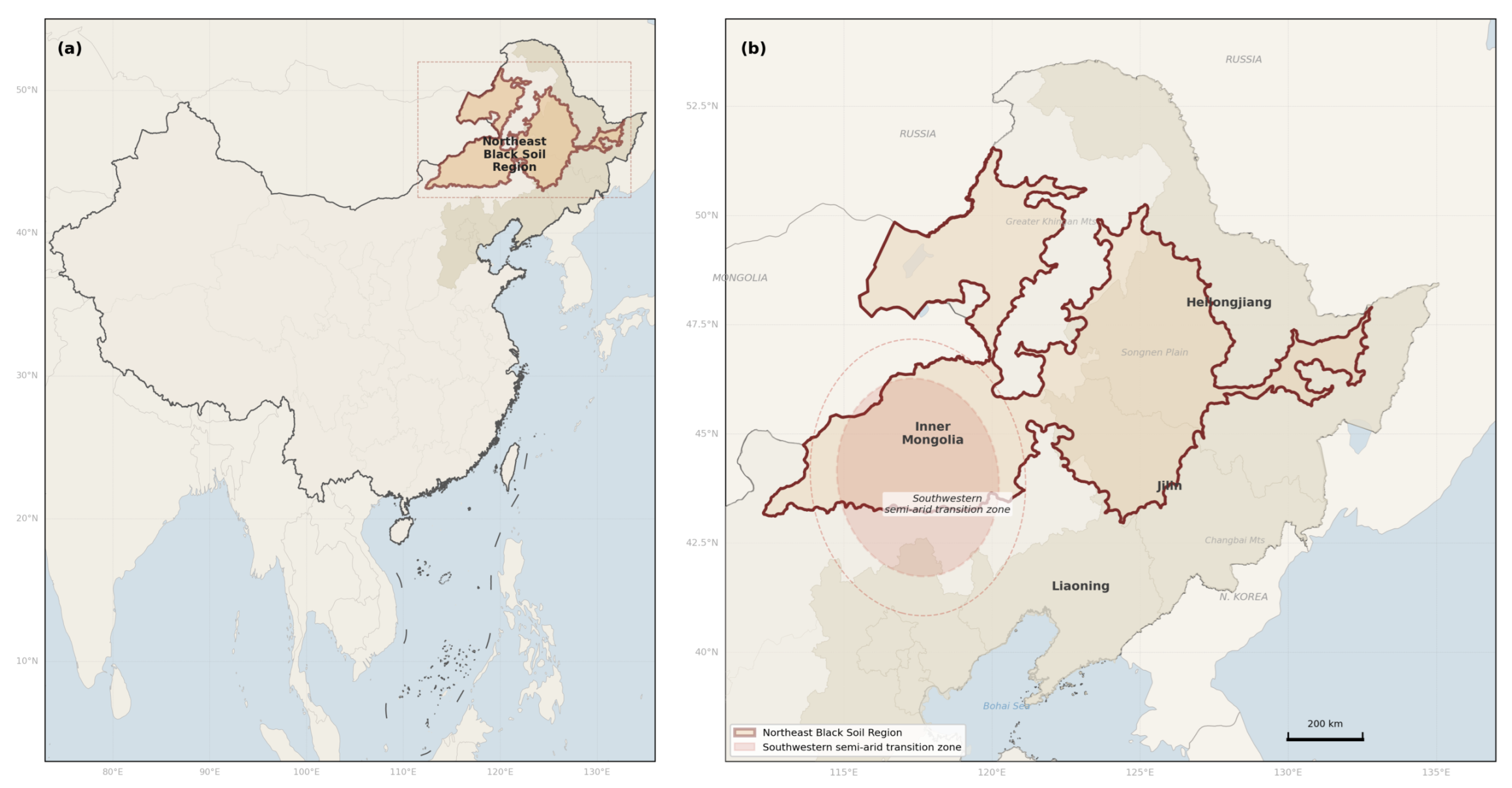
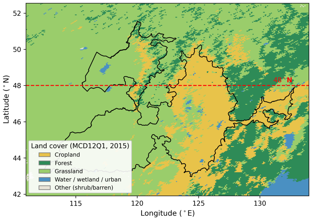
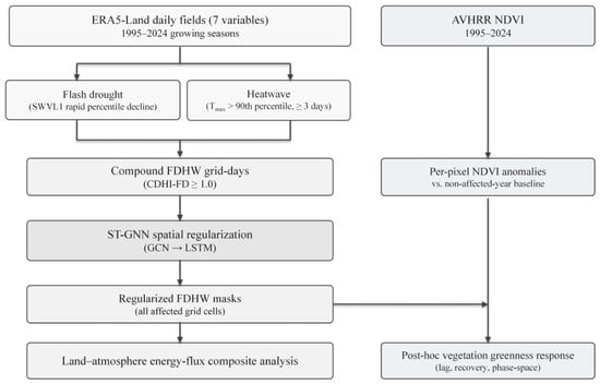
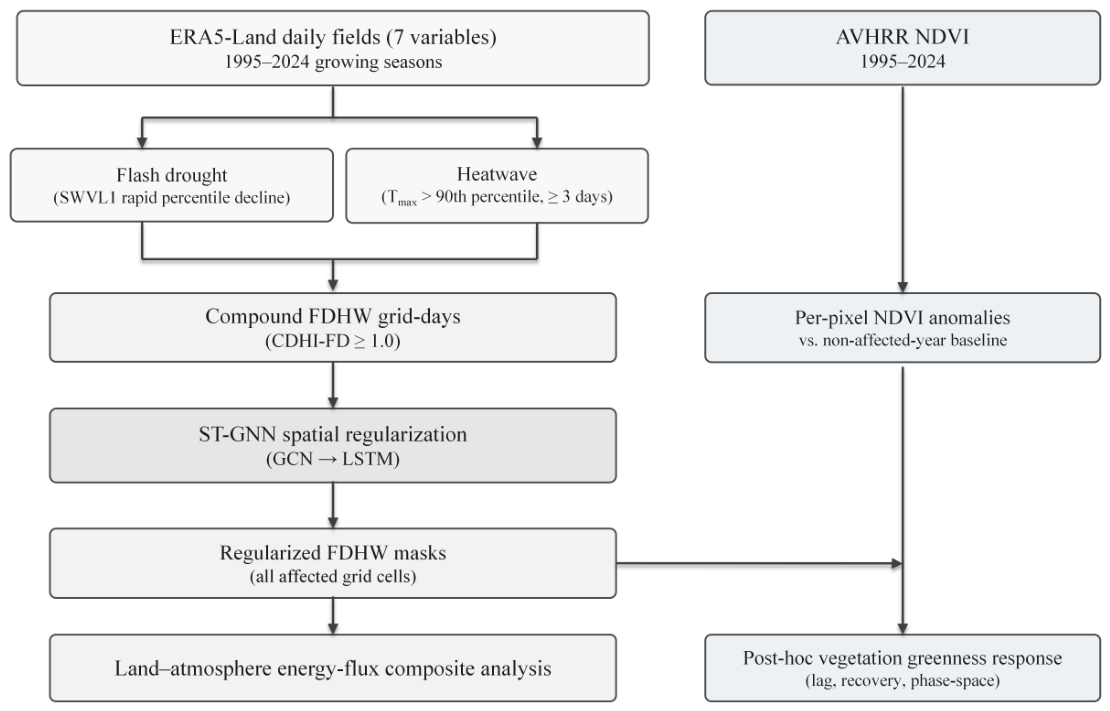
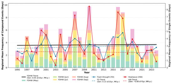
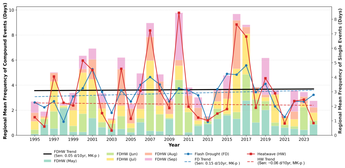
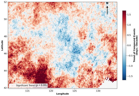
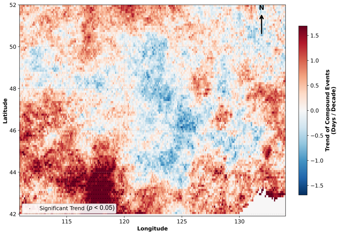
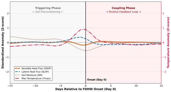
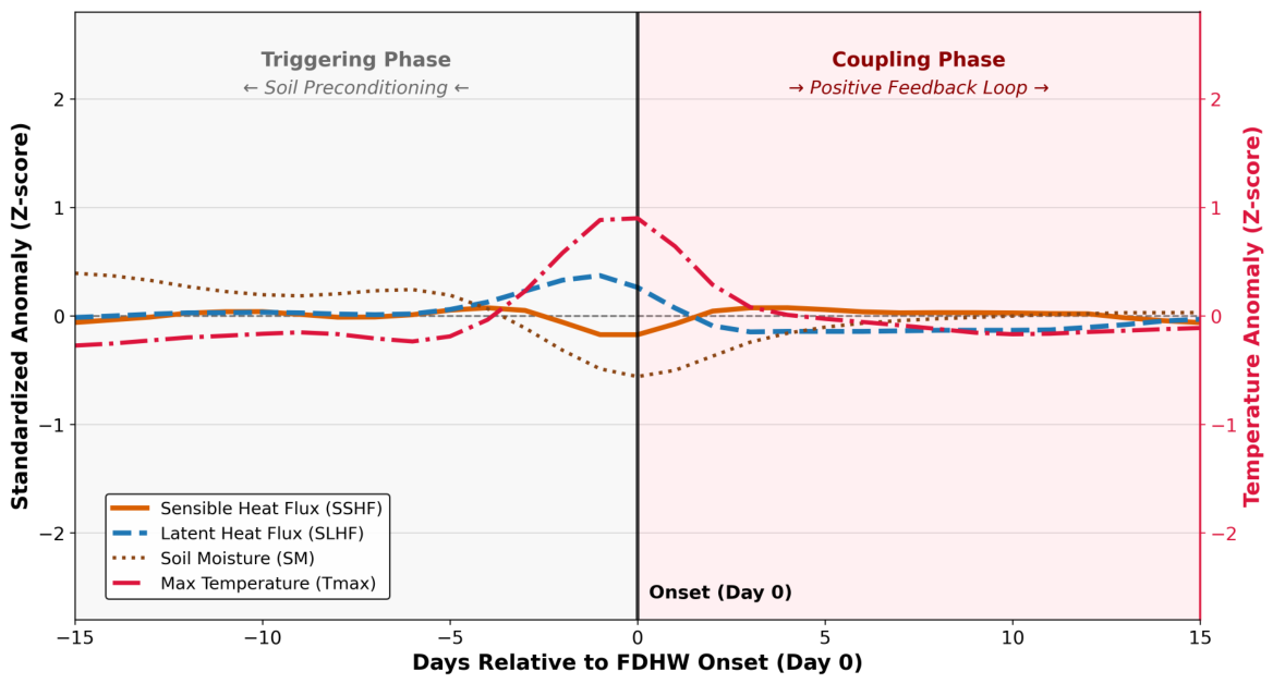
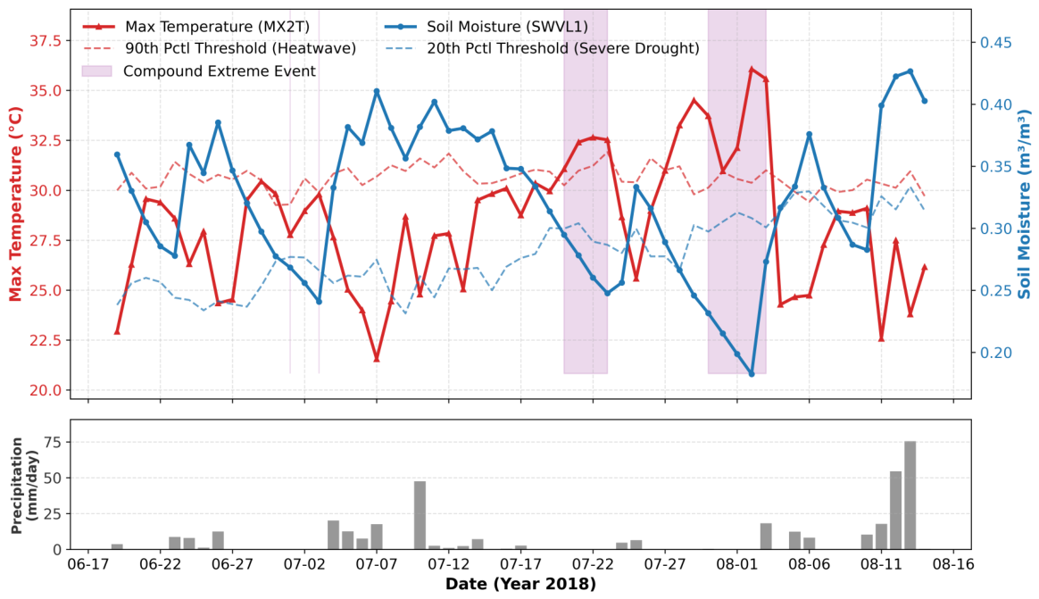
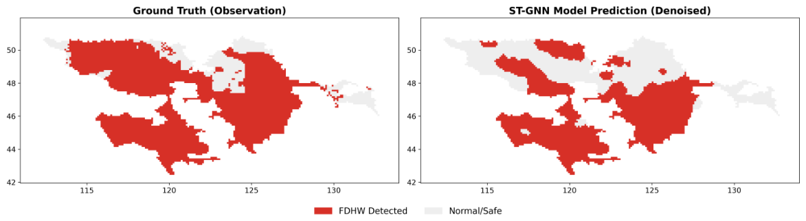
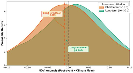
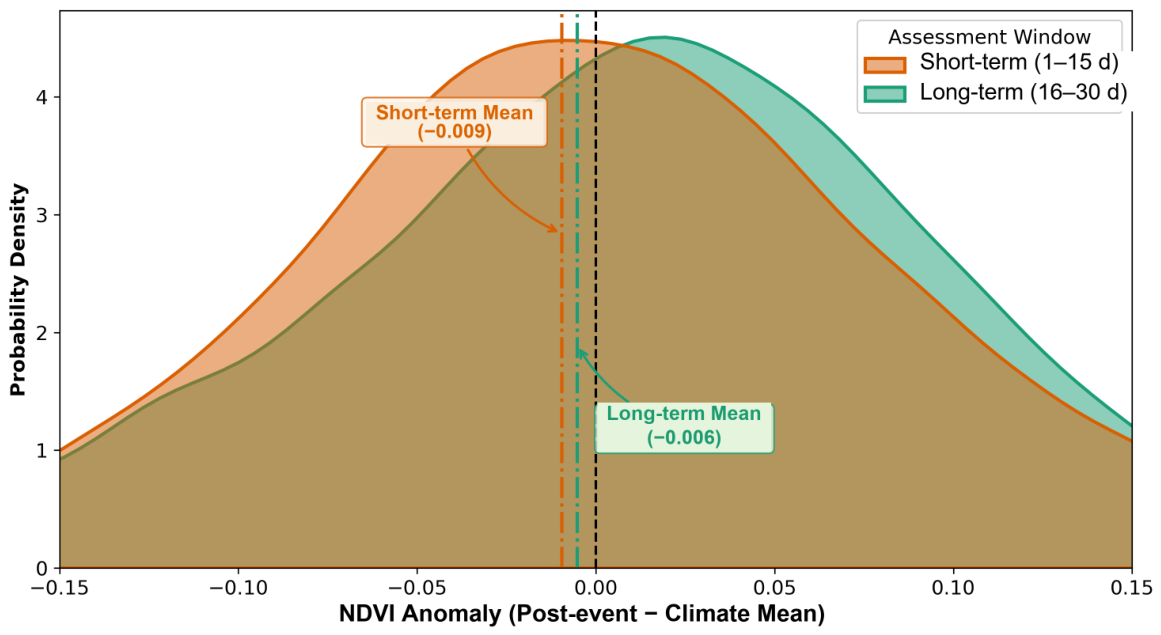
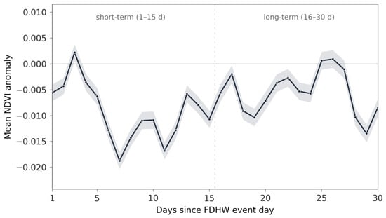
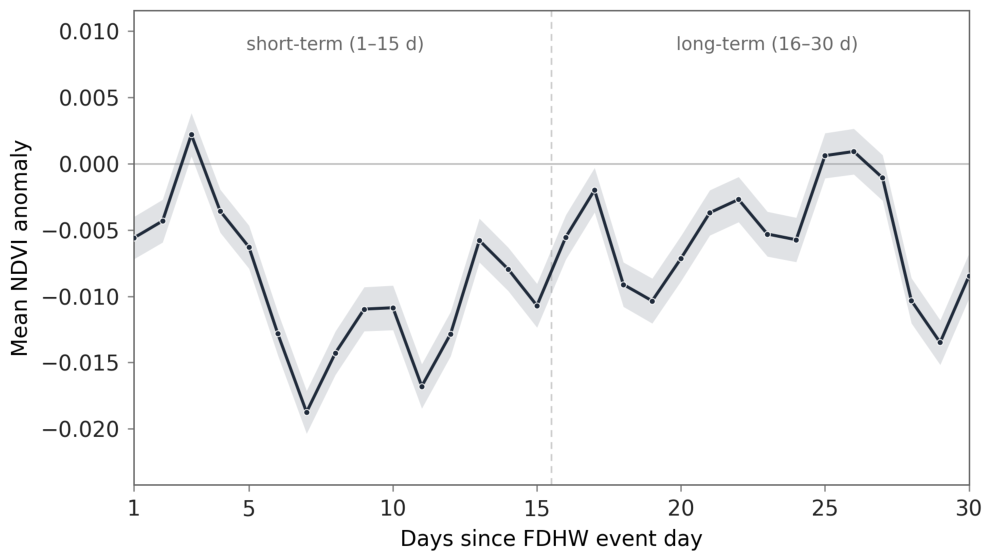
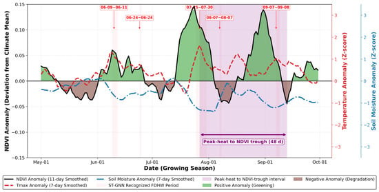
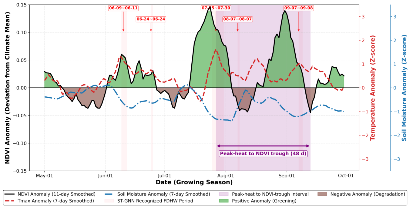
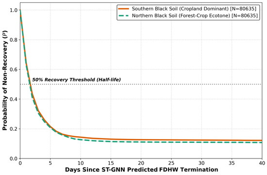
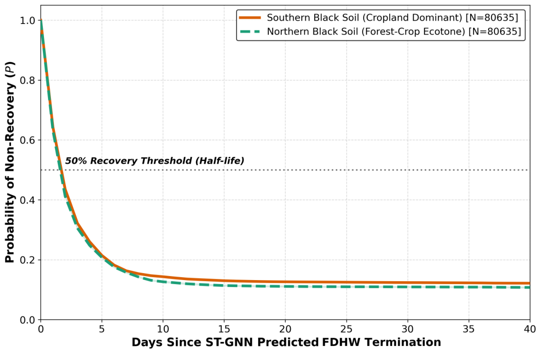
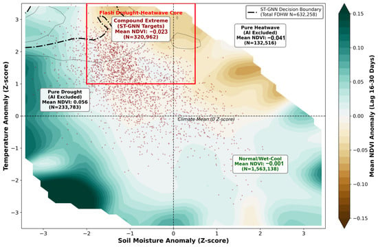
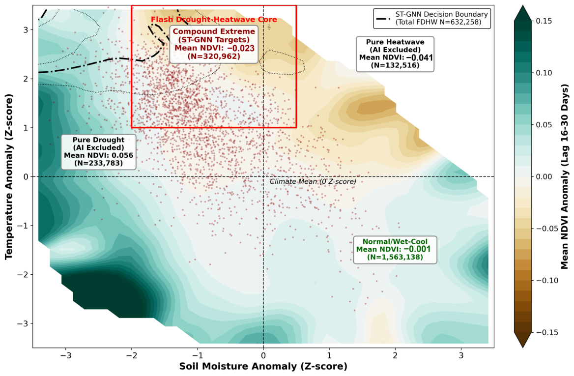

Disclaimer/Publisher’s Note: The statements, opinions and data contained in all publications are solely those of the individual author(s) and contributor(s) and not of MDPI and/or the editor(s). MDPI and/or the editor(s) disclaim responsibility for any injury to people or property resulting from any ideas, methods, instructions or products referred to in the content. |
© 2026 by the authors. Licensee MDPI, Basel, Switzerland. This article is an open access article distributed under the terms and conditions of the Creative Commons Attribution (CC BY) license.