


Highlights
What are the main findings?
- The integration of temporal–spectral–spatial features can comprehensively characterize epileptic signals from multiple perspectives, effectively enabling the construction of seizure prediction models by combining multiple deep learning methods.
- The dynamic multigraph attention network based on time slices can flexibly adapt to feature patterns of multiple channels and frequency bands, utilizing a unified graph network to achieve overall interaction across frequency bands, thereby obtaining comprehensive spatial features.
What are the implications of the main findings?
- Comprehensive performance based on both segment-based and event-based evaluations demonstrates the reliability of the model.
- The patient-specific experiments verify the effectiveness of the model in achieving personalized prediction. In contrast, the patient-independent experiments demonstrate the model’s strong generalization ability on unseen subjects.
Abstract
Background/Objectives: Epilepsy is a recurrent cerebral disorder, and the sudden onset of seizures can result in accidental injuries or even life-threatening events for patients. In clinical practice, epileptic seizure prediction can provide warnings prior to the onset of seizures, alerting patients to take safety precautions and assisting neurologists in implementing timely interventions to suppress seizures. Therefore, accurate prediction is crucial for improving patients’ quality of life and clinical treatment outcomes. However, due to insufficient extraction of effective features from epileptic signals, the performance of prediction models is often limited. Methods: In this study, a novel deep learning model was proposed that integrated temporal–spectral–spatial features to address this limitation. Wavelet convolutions and temporal convolutions were employed to achieve the temporal–spectral representation network. Subsequently, the fused features were further processed using bidirectional long short-term memory networks and a dynamic multigraph attention network based on time slices to extract temporal and spatial features for seizure prediction. Results: The performance of the proposed model was comprehensively evaluated on the CHB-MIT and Siena databases using both segment-based and event-based evaluations. For the CHB-MIT database, the model achieved a sensitivity of 96.09 ± 8.83% and a false prediction rate of 0.021 ± 0.032/h. For the Siena database, the model demonstrated a sensitivity of 95.71 ± 7.87% and a false prediction rate of 0.028 ± 0.036/h. Furthermore, this study achieved patient-independent experiments for prediction evaluation. Conclusions: The proposed model effectively achieves the fusion of multiple features and significantly enhances the prediction performance through multiple deep learning methods. For patient-independent experiments, the excellent prediction performance demonstrates the strong generalization ability.
1. Introduction
Epilepsy is a neurological disorder characterized by recurrent and transient seizures, primarily caused by abnormal electrical activity in the brain [1]. The etiologies of epilepsy encompass a variety of factors, including cortical dysplasia, brain tumors, traumatic brain injuries, cerebral malformations, central nervous system infections (e.g., tuberculous meningitis, neurosyphilis, viral meningitis), and parasitic infections (e.g., cerebral cysticercosis) [2]. The pathogenesis of epilepsy is highly complex, primarily related to abnormalities in ion channel function, neurotransmitter regulation, and glial cell dysfunction. Clinical manifestations of seizures may include momentary loss of consciousness and collapse, abnormal sensory perceptions, hallucinations, repetitive utterances of words or syllables, and rotational movements of the body or eyes [3]. Upon seizure termination, some patients can immediately recover to a normal state, while others may take several minutes or hours to recover. According to the World Health Organization, there are approximately 50 million epilepsy patients worldwide, and the risk of premature death is three times higher compared to the general population [4]. The significant proportion of deaths is attributable to preventable causes such as falls, drownings, burns, and prolonged seizures.
Epileptic seizures exhibit stereotypical patterns, leading to similar manifestations and symptoms corresponding to abnormal brain discharge regions [5,6]. Based on this characteristic, it is possible to predict epileptic seizures and send early alarms to patients and clinicians prior to the onset of seizures. Epileptic seizure prediction offers several benefits: (1) it reduces the risk of accidental injuries by allowing patients to take preventive measures, such as moving away from dangerous environments or lying down, thereby minimizing falls, burns, or choking due to tracheal obstruction [7]; (2) it optimizes treatment strategies, as warnings enable patients to follow medical instructions, such as administering antiepileptic drugs, avoiding visual stimuli, or practicing deep breathing exercises to suppress seizures or alleviate symptoms [8]; (3) it facilitates precise interventions (e.g., medication adjustments, deep brain stimulation) based on brain lesion localization to effectively disrupt seizure progression and reduce cumulative cognitive impairment caused by frequent seizures [9]; (4) it improves patients’ quality of life through early warnings, which can alleviate patients’ anxiety and depression while enhancing their sense of disease control and mental health; (5) it advances epilepsy research and deepens pathological understanding, as prediction technologies reveal dynamic patterns in brain electrical activity prior to seizures, providing new insights into the initiation, propagation, and termination mechanisms of abnormal neuronal discharges [10,11,12]; and (6) it promotes the development of management mechanisms, transitioning epilepsy treatment from passive response to proactive prevention, making it a manageable risk [13]. Therefore, achieving accurate and timely epileptic seizure prediction constitutes a critical research focus for epilepsy prevention and treatment.
Electroencephalogram (EEG) signals capture the variations in electrical waves generated during brain activity, which reflect the electrophysiological functions of neuronal cells in the cerebral cortex or scalp surface. EEG signals are widely used in clinical epilepsy diagnosis and treatment. Epileptic signals can be divided into four different stages: during the interictal period, EEG signals typically show normal or only mild abnormalities without obvious symptom features; in the preictal stage, EEG signals begin to exhibit abnormalities, manifested as changes in specific frequencies or waveforms, indicating that a seizure is imminent; during the ictal period, EEG signals show significant abnormalities, accompanied by typical epilepsy symptoms; and in the postictal stage, EEG signals gradually return to normal and consciousness is restored [14]. The waveform schematic diagram of four stages of epileptic signals is shown in Figure 1. Epileptic seizure prediction is commonly achieved by distinguishing between interictal and preictal signals, in order to issue timely warnings during the preictal stage [15]. EEG acquisition methods are divided into scalp EEG and intracranial EEG (iEEG) [16]. Scalp EEG involves placing electrodes on the scalp surface, connected via wires to EEG devices to record cortical electrical activity, providing a non-invasive and convenient approach; whereas iEEG requires surgical implantation of electrodes directly into the skull, positioned on the surface or inside of the cerebral cortex, allowing for more direct recording of neuronal electrical activity. Given that epileptic seizure prediction necessitates long-term measurement of patients’ EEG signals with the requirement for safe, non-invasive, and wearable devices, scalp EEG is mainly employed in epileptic seizure prediction. In clinical practice, achieving seizure prediction requires clinicians to conduct prolonged visual inspections and confirm signal states. This process is time-consuming and prone to misdiagnosis due to subjective interpretation. These limitations have rendered the development of effective seizure prediction algorithms an urgent clinical necessity.
Figure 1.
The waveform schematic diagram of four stages of epileptic signals.
In early studies on seizure prediction, algorithms lacked integration of artificial intelligence techniques. During this period, short-term maximum Lyapunov exponent and smoothed spike rate were employed as indicators, with alerts being triggered when these metrics exceeded statistical thresholds [17,18]. These threshold-based prediction methods demonstrate high computational efficiency and ease of implementation but exhibit relatively low prediction performance. To improve the predictability of algorithms and adapt them to the current large-scale datasets, machine learning approaches have been widely adopted in seizure prediction research [19]. Machine learning methods typically require feature extraction and selection from raw data, followed by training classifiers using labeled datasets to achieve seizure prediction. However, these approaches have limitations in processing raw data, often necessitating manual extraction of appropriate features from epileptic signals through researchers’ accumulated experience and extensive experimentation. These methods heavily depend on the individual expertise and knowledge reserves of researchers. Since deep learning methods can automatically extract effective features and learn complex model structures to avoid relying on manually engineered feature extraction and reduce the possibility for subjective human intervention, the application of deep learning techniques in seizure prediction has emerged as a new research trend [20].
Considering the rich information contained in epileptic signals, a novel deep learning model is proposed in this study. The spectral and temporal features are respectively extracted using wavelet convolutions and temporal convolutions. Subsequently, the temporal and spatial features are deeply extracted by employing bidirectional long short-term memory (BiLSTM) networks and a dynamic multigraph attention network based on time slices (DMAN-TS). The acquired temporal–spectral–spatial features are fused to achieve comprehensive representation of epileptic signals. The integration of differentiable pooling (DiffPool) effectively compresses the graph scale and learns multi-granular hierarchical features. Two public databases are employed to evaluate the prediction performance. The primary contributions of this work can be summarized as follows:
- This study extracts the temporal–spectral–spatial features using multiple deep learning methods and achieves comprehensive representation of epileptic signals through multi-feature fusion.
- This study proposes a novel DMAN-TS method that effectively combines feature patterns of multiple channels and frequency bands. The utilization of parallel edges enables the unified mapping of multi-band features into a single graph and facilitates overall interaction. By incorporating spatial coordinate systems, spatial feature extraction can learn more precise physical mapping relationships.
- This study utilizes two public databases to evaluate the prediction performance, employing both segment-based and event-based evaluations for a more comprehensive assessment. The excellent prediction results demonstrate the robust generalization capability and reliable outcomes. This study further evaluates the prediction performance of patient-independent experiments to emphasize the generalizability on unseen subjects.
2. Related Works
Research on epileptic seizure prediction is devoted to developing advanced and effective algorithms to identify the preictal state, thereby enabling timely and reliable alerts for imminent seizures and guiding clinicians in determining the appropriate time for taking antiepileptic drugs and neural stimulation interventions. To achieve this objective, early research utilized machine learning approaches to analyze large-scale datasets for epileptic seizure prediction. Zhong et al. employed fuzzy entropy, power spectral density, and brain networks to deeply explore the spatiotemporal characteristics of epileptic signals [21]. Subsequently, support vector machines were used to classify the signals. The method combined a majority voting mechanism as a post-processing algorithm, achieving satisfactory discriminative performance and providing a valuable framework. Ra et al. adopted the synchroextracting transform and sparse representation for feature extraction, followed by classification of the interictal and preictal periods using the k-nearest neighbor classifier [22]. This research demonstrated promising performance in time-frequency representation, providing a potential prediction method.
Due to the limitations of machine learning methods that heavily rely on manual feature engineering and their weak ability in handling complex data, many deep learning methods have recently been applied to seizure prediction. Liu et al. utilized temporal, spatial, and frequency information to achieve seizure prediction by combining a convolutional neural network (CNN) and a long short-term memory (LSTM) network [23]. This study provided a potential solution for the development of wearable devices. Yang et al. proposed a lightweight triscale-yielding CNN to capture multi-scale complex signal features, providing insights for lightweight design [24]. Yue et al. proposed an augmented EEG Transformer model to effectively extract multi feature information from EEG data [25]. Zhang et al. introduced the implementation of seizure prediction using the Siamese network and triplet network, which was composed of a tiny CNN and supervised contrastive learning [26]. Although satisfactory performance was achieved, the use of an excessive number of channels limited the scalability of the algorithm. Shan et al. utilized an interpretable multi-branch architecture of a spatiotemporal CNN to achieve seizure prediction [27]. This research achieved excellent performance. However, the algorithm’s consideration of test results for a single database limited its application across databases. The current research only considers the segment-based evaluation and lacks consideration for the event-based evaluation. The event-based evaluation, which aligns with the clinical stages of seizure progression, is crucial for clinicians to clarify the mechanisms and processes of epileptic seizures. Furthermore, the event-based classification can provide a more intuitive identification of seizure stages, promote the development of intervention strategies tailored to individual patterns, and enhance the adaptability of epilepsy management.
Patient-specific experiments, in which models are trained individually for each patient, are capable of fully considering inter-individual differences to better meet personalized needs and improve the specificity and effectiveness of treatments. Feizbakhsh et al. extracted the densities of data in each cluster as features and input them into both random forest (RF) and CNN classifiers to achieve seizure prediction [28]. The results indicated better classification performance of CNN compared to RF. However, this study was limited by the small number of seizure events analyzed. Rao et al. employed sample entropy and anchoring temporal convolutional networks for seizure prediction [29]. This algorithm achieved a prediction time exceeding the onset of antiepileptic drugs by extracting temporal causal relationships, thereby enabling timely intervention to prevent seizures. However, the prolonged seizure occurrence period tended to induce tension and anxiety in patients. Wang et al. employed a channel reordering strategy and a CNN-LSTM framework for seizure prediction [30]. The algorithm was validated on iEEG databases and achieved promising prediction performance. However, the lack of testing on scalp EEG databases limited its application to non-invasive and wearable devices. Qi et al. utilized robust feature representations and a vision transformer for seizure prediction [31]. A channel selection layer was incorporated to effectively identify EEG channels with significant contributions to classification performance. The current methods mainly overlook research of patient-independent experiments. Patient-independent experiments aim to develop a highly applicable universal prediction model that can learn common characteristics of epileptic seizures, thereby improving the prediction performance of new patients. Since training models individually for each patient consumes substantial computational resources, it is clinically necessary to investigate the classification performance of the model on unseen subjects to verify its generalization ability.
With the gradual development of deep learning methods, using these techniques to extract features has emerged as a predominant research direction in seizure prediction. Dong et al. employed the stockwell transform and multi-channel vision transformer to identify seizure states by extracting spectrograms and spatial features [32]. This method demonstrated potential applicability in predicting seizures for drug-resistant epilepsy patients. However, the utilization of an excessive number of EEG channels in this study might pose challenges to hardware deployment. Xia et al. extracted multi-layer time-frequency features and employed LSTM and transformer networks to achieve good classification performance [33]. Al Musafir et al. used graded spiking neural networks for seizure prediction and deployed a neuromorphic processor for hardware deployment [34]. Liu et al. extracted multi-domain EEG features and input them into a multi-scale convolutional network for classification, providing a possible framework for clinical applications [35]. Qu et al. utilized a dilated causal convolutional network to obtain local features and applied causal attention mechanisms to extract global correlation features for seizure prediction, thereby guiding clinicians in taking antiepileptic drugs [36]. Current research lacks the application of a graph neural network (GNN). GNN is more adept at capturing global topological relationships through a message-passing mechanism involving neighbor aggregation and node updates. GNN utilizes the information conductivity of graphs to improve feature extraction capabilities and model performance.
Compared with other studies, this paper effectively extracts fused temporal–spectral–spatial features using CNN, BiLSTM, and DMAN-TS. This study achieves comprehensive representation of epileptic signals and improves prediction performance by combining multiple deep learning methods. This work uses two databases to evaluate the model’s prediction performance through both segment-based and event-based evaluations, effectively alleviating the limitations of insufficient metrics caused by a single-method evaluation. Additionally, both patient-specific and patient-independent experiments are conducted. The patient-independent experiments demonstrate the strong generalization ability of the model on unseen subjects.
3. Materials and Methods
3.1. Epileptic EEG Databases
The first database is the CHB-MIT scalp database collected at the Children’s Hospital Boston [37]. This database comprises EEG records of 23 pediatric patients following the withdrawal of antiepileptic drugs. These records were divided into 24 cases based on the subjects, with case 1 and case 21 originating from the same subject. Each case provided files detailing the electrode positions and seizure timing information. All records were obtained using the international 10–20 system at a sampling rate of 256 Hz. Due to the variability in the number of seizures and seizure duration across cases, the data selected for analysis were required to meet three criteria: (1) only the first seizure was considered in cases of multiple seizures within 30 min; (2) the total interictal interval duration of each case was at least 3 h; and (3) each case involved at least three seizures. Data that did not satisfy these criteria were excluded from the study. Detailed information regarding the subjects used in the CHB-MIT database is summarized in Table 1.
Table 1.
Detailed information regarding the subjects used in the CHB-MIT database.
The second database is the Siena scalp database collected at the University of Siena [38]. This database includes EEG records from 14 epilepsy patients who were monitored using video-EEG with a sampling rate of 512 Hz. The electrodes were arranged according to the international 10–20 system. Each patient provided files containing electrode location and seizure information. Data selection followed the previous criteria, but due to the relatively short duration of records in this database, the total interictal duration of each case was at least 1.5 h. Detailed information regarding the subjects used in the Siena database is presented in Table 2.
Table 2.
Detailed information regarding the subjects used in the Siena database.
The CHB-MIT database exhibited inconsistencies in electrode configurations across cases because certain electrodes were not utilized in some subjects. In contrast, the Siena database uniformly employed 29 electrodes. To avoid inconsistencies caused by differences in electrode positions, this study selected electrode positions common to all subjects in both databases for analysis. Furthermore, to optimize computational complexity, the selected electrode positions included FP1, F3, C3, P3, O1, FZ, CZ, PZ, F4, C4, P4, O2, FP2, F8, and F7.
3.2. The Proposed Approach
The proposed model employs deep learning approaches to fuse the extracted temporal–spectral–spatial features to achieve comprehensive signal representation and effectively provide discriminative features for seizure prediction. The structure of the proposed model is illustrated in Figure 2.
Figure 2.
The structure of the proposed model.
Initially, the epileptic signals are fed into the temporal–spectral representation network. Wavelet convolutions are used to extract spectral features based on EEG frequency bands, while temporal convolutions are used to extract temporal features embedded in time-series signals. Subsequently, the spectral and temporal features are fused according to different frequency bands and transmitted to both BiLSTM and DMAN-TS networks. The BiLSTM network extracts bidirectional long-distance dependencies from five frequency bands. The output features are obtained by performing average pooling on the output of the last time step for each frequency band, enabling attention to temporal patterns across bands. The DMAN-TS network extracts spatial features by treating the five frequency-band features as parallel edges, enabling the exploration of evolutionary patterns in the spatial structure across time slices. Additionally, the network can autonomously learn the significance of neighboring nodes and assign different weights for information fusion to enhance feature representation capabilities. The spatial features are then transmitted to two layers of DiffPool networks and global average pooling to achieve hierarchical graph representation learning and obtain graph-level representations. Finally, the obtained graph-level representations and the temporal output features from the BiLSTM network are fused and transmitted to the fully connected layer and post-processing module to complete the seizure prediction task. When the model identifies the preictal state, an alarm is immediately triggered to guide patients and clinicians in taking relevant preventive measures.
3.2.1. Temporal–Spectral Representation Network
To facilitate detailed analysis of the information contained in different frequency bands, clinical EEG signals can be divided into five distinct frequency sub-bands: δ band (0–4 Hz), θ band (4–8 Hz), α band (8–13 Hz), β band (13–30 Hz), and γ band (>30 Hz). The neuronal activities of epilepsy patients exhibit different frequency patterns, which may manifest as rhythmic disturbances (e.g., increased slow waves, abnormal background rhythm) or high-frequency bursts (e.g., spikes, sharps) exceeding the background activity. In this study, multi-resolution spectral features and multi-scale temporal features are extracted from epileptic signals across sub-bands by employing the hierarchical wavelet convolution (WaveConv) and temporal convolution.
Wavelet convolution represents an approach that integrates wavelet transforms with deep convolutional neural networks, aiming to enhance the receptive field and low-frequency feature extraction ability of convolutional layers through multi-resolution decomposition and frequency analysis. The core concept involves the utilization of wavelet transforms to decompose feature maps into different frequency sub-bands, followed by convolution operations performed on each sub-band to effectively capture global contextual information. This method is widely applied in various fields, including analysis of time-series data, image classification, and action recognition.
The Daubechies series of wavelets possesses compact support and orthogonality, with smooth waveforms and a strong ability to capture details. Therefore, the Daubechies order-4 (Db4) wavelet is used to process epileptic signals with high correlation. In this study, predefined wavelet filters are employed as convolutional kernels, with fixed weights assigned to these kernels. Specifically, for the epileptic signals xl, the wavelet convolution is defined as:
where and are approximation and detail coefficients, respectively. k and s represent the kernel size and stride in the convolution operation. Ψ(k) and φ(k) denote the approximation and detail filters, respectively. Based on the Db4 wavelet, k is 8, and s is 2. The obtained parameter can be further propagated into the next wavelet convolution layer to perform L-layer iterative analysis. According to the data sampling rate Fs and the five frequency bands used, L is 5. Through the above method, the frequency boundaries of and are (0,Fs/2l+1) and (Fs/2(l+1),Fs/2l), respectively, where l = 1, 2,…,L. Consequently, multi-resolution spectral features of five frequency bands are successfully extracted.
Temporal convolutions can effectively extract multi-scale features from temporal patterns. The proposed approach uses five parallel temporal convolutional layers to construct the temporal representation. To maintain consistency with the feature representations of frequency bands obtained from wavelet convolutions, kernel sizes and strides corresponding to δ, θ, α, β, and γ are set as 32, 32, 16, 8, and 4, respectively. Each temporal convolutional layer is followed by batch normalization and an exponential linear unit to improve model training stability and accelerate convergence. Subsequently, spectral and temporal features are concatenated channel-wise to obtain the temporal–spectral representation network of five frequency bands.
3.2.2. BiLSTM
When recurrent neural networks (RNNs) learn from long sequences, they are prone to the phenomena of gradient vanishing and explosion. Therefore, RNNs cannot capture long-term nonlinear relationships, resulting in the inability to learn long-term dependencies. LSTM is proposed to address these problems. LSTM can retain and forget previous input information through internal gate mechanisms to maintain and update cell states. LSTM includes an input gate, a forget gate, and an output gate.
The formulas of the LSTM are described as:
where ht−1 and xt are the hidden layer’s state and the input data, respectively. ft, it, ot are states for the forget gate, the input gate, and the output gate, respectively. Wf, Wi, Wg, Wo are the weights. bf, bi, bg, bo are the bias terms. gt and ct are the candidate memory cell and the memory cell state, respectively. ht is the hidden layer’s output. sig is the sigmoid activation function. tanh is the hyperbolic tangent activation function. ⊗ stands for the Hadamard product.
The input gate controls the information quantities of the candidate memory cell gt that need to be saved on the memory cell state ct. The forget gate can map values to the interval (0, 1) through the sigmoid activation function. These values determine the information to be reserved or forgotten on the memory cell state ct−1, where one represents completely retaining information and zero represents completely forgetting information. The output gate controls the amount of information stored on the memory cell state ct that needs to be transmitted into the output ht.
BiLSTM can enhance the logic of data structures by simultaneously modeling input sequences forward and backward, making the network architecture contain both past and future information. BiLSTM can retain the structural characteristics of the LSTM unit and make up for the inability of LSTM to simultaneously capture the characteristic information from back to front. Therefore, BiLSTM can more abundantly learn long-term dependencies. The diagram of the BiLSTM structure is illustrated in Figure 3.
Figure 3.
The diagram of the BiLSTM structure.
The updated formulas of BiLSTM are described as:
where xt denotes the input data. , , , are hidden layer’s states and memory cell states for forward and backward layers. ht denotes the output of BiLSTM. In this study, in order to obtain a fixed length representation of the entire sequence, we use the output tensor of the last time step T as the output feature of BiLSTM.
3.2.3. DMAN-TS
The positions of EEG electrodes contain spatial information, and a spatial representation of channel mapping can be constructed based on these electrode positions. In this study, we utilize the three-dimensional (3D) positions of electrodes from the international 10–20 system to precisely measure the distances between different electrodes for constructing a spatial network. The Euclidean distance between electrode i and j is denoted as dij, where i,j ∈ {1, 2,…,C}, and C denotes the number of electrodes. To characterize the overall connectivity between electrodes, a distance set is constructed and represented as H = {dij|i,j ∈ [1,C],i ≠ j}. Additionally, AVE(H) is defined as the average distance within set H. To accurately characterize the connectivity relationships and their intensities between electrodes, a distance-based adjacency matrix Ainit ∈ RC×C is constructed, defined as follows:
The adjacency matrix constructed above depends on a fixed electrode distance and cannot construct heterogeneity across subjects. This study employs the squeeze-and-excitation (SE) mechanism to construct a dynamic adjacency matrix, enabling the learning of whether connections between electrodes should be emphasized or suppressed through training, and models the dependencies between EEG signals. The structure of the SE mechanism is illustrated in Figure 4.
Figure 4.
The structure of the SE mechanism.
The input of the SE mechanism is , and FSE denotes the EEG sequence. Firstly, each electrode’s information is compressed into a scalar through the squeeze operation. Global average pooling is applied to sequence signals of the input XSE to obtain z ∈ RC, which aggregates the global temporal response of each electrode. Subsequently, the excitation operation is utilized to learn nonlinear transformations for generating adaptive weights for each electrode. It employs two fully connected networks and nonlinear functions. The first layer serves for dimensionality reduction, denoted as:
where W1 ∈ R(C/r)×C, r represents the reduction rate, and the output h1 ∈ RC/r. The purpose of dimensionality reduction is to enforce the model to learn compact dependencies between electrodes and prevent overfitting. The second layer is designed for dimensionality expansion, denoted as:
where W2 ∈ RC×(C/r), the output s ∈ RC, and s denotes electrode importance weights. Subsequently, based on prior constraints of brain anatomical connections, preserving the topology of Ainit without generating false connections that do not conform to physiological structures, bilateral modulation is used to generate the dynamic adjacency matrix. The formula is defined as follows:
where diag(s) ∈ RC×C represents a diagonal matrix and A ∈ RC×C denotes the dynamic adjacency matrix.
GNN is a deep learning approach used for graph data processing, which models a set of objects and their interrelationships. In the graph, objects represent nodes, while relationships represent edges. Due to the powerful representational ability of graph structures, GNN is widely used in research on node classification, graph classification, and relationship prediction. Graph attention network (GAT) is a neural network specifically designed for processing graph-structured data. Its core lies in introducing an attention mechanism that automatically assigns weights to different neighboring nodes, thereby identifying more significant adjacent nodes and more accurately capturing and expressing the relationships between nodes. Based on the dynamic adjacency matrix constructed above, GAT can further learn the discriminative importance of various neighbors, making the aggregated features of nodes more aligned with task requirements.
In this study, a dynamic multigraph attention network based on time slices (DMAN-TS) is employed for epileptic seizure prediction. By adaptively learning the importance weights between nodes, DMAN-TS focuses on high-value dynamic correlation features. The continuously evolving dynamic networks are segmented into a sequence of static graph snapshots over a fixed length of time, forming an ordered sequence:
where the multigraph G(t) at each time slice t ∈ {1, 2,…,T} is defined as:
where V(t) denotes the set of nodes at time slice t. E(t) denotes the set of undirected edges. Since a multigraph allows parallel edges between the same pair of nodes, E(t) represents a multiset. (i,j) ∈ E(t) represents the presence of at least one parallel edge between nodes i and j. F(t) denotes the set of edge features and defines as , where denotes the number of parallel edges between the pair of nodes (i,j), and denotes the feature vector of the k-th parallel edge. In this study, electrodes represent nodes in the graph network. Node features use clustering coefficients and shortest path lengths, while edge features use the output of the temporal–spectral representation network.
The initial input feature vector of node i is denoted as . To enable the model to learn better feature representations while allowing for flexible adjustment of the output feature dimensions, a shared weight matrix is applied for linear transformation to map features to a new feature space:
where is the learnable weight matrix, and d′ represents the dimension of the transformed features. To preserve the complete differences between parallel edges, the attention score of each edge is independently calculated. Additionally, separate learnable parameters are used for different edge types. For the k-th parallel edge between node i and its neighbor j, the attention score is calculated as:
where represents the learnable attention vector specific to the k-th edge type. [⋅‖⋅] denotes the vector concatenation operation.
Apply the softmax function to normalize all neighboring nodes of node i and all its parallel edges, obtaining normalized attention weights, defined as:
where N(t)(i) ∪ {i} denotes the neighbor set of nodes i plus itself. Additionally, N(t)(i) = {j ∈ V(t)∣(i,j) ∈ E(t)}. The normalization denominator iterates over all neighbors u and all parallel edges k′, ensuring that each edge in the multigraph independently participates in attention competition without interfering with each other.
In the process of message passing, each parallel edge generates messages independently, and different edge types utilize separate transformation matrices. The formula for message generation is described as:
where represents the message transformation matrix dedicated to the k-th edge type.
The updated features of node i are obtained by weighted summation of all parallel edge messages from all neighbors based on their attention weights. To improve model stability and the richness of feature capture, a multi-head attention mechanism is introduced. Specifically, M independent attention heads are executed in parallel, and their results are averaged to obtain the new feature representation of node i at time slice t:
where σ(⋅) denotes a nonlinear activation function.
The above process completes the feature aggregation within a single time slice. To capture dynamic evolution, the embedding sequences of each node across time slices are fed into a multi-head self-attention network for temporal modeling. This allows the model to automatically learn the dependencies between different time slices, enabling it to better focus on the most relevant nodes and connections in the graph. The temporal feature matrix of node i is constructed by stacking the embeddings of T time slices:
To learn different dependency patterns in low-dimensional subspaces, a multi-head attention mechanism is employed to parallelly compute multiple attention heads. L denotes the number of heads, dhead = d′/L denotes the dimension of each head. For the l-th head, three independent weight matrices are utilized to project the input into query, key, and value spaces:
where denotes the learnable weight matrices.
The scaled dot-product attention is computed for the l-th head:
The outputs of all heads are concatenated along the feature dimension and subsequently transformed through a linear transformation to obtain the updated representation:
where ensures the output matrix has the same dimension as the input Xi.
To improve training stability, the residual connection and layer normalization are applied after the multi-head attention mechanism:
Subsequently, global average pooling is performed to acquire node representations that integrate global temporal dependencies:
3.2.4. DiffPool
To obtain a comprehensive representation of the entire graph, it is necessary to use graph pooling techniques to aggregate information from various nodes and preserve graph structural details. Differentiable pooling (DiffPool) clusters the nodes of the original graph into fewer super nodes based on a learned assignment matrix, resulting in a new graph after graph coarsening and achieving hierarchical graph representation learning. DiffPool can gradually compress the graph scale, reduce computational complexity, maintain the graph topological structure, avoid the loss of key node information, and learn multi-granularity hierarchical features of the graph. This method is widely used in graph classification tasks.
The initial node feature matrix is obtained by aggregating the features of all C nodes. The adjacency matrix of the last time slice is taken as the initial adjacency matrix A(0) ∈ RC×C. A total of M DiffPool layers are defined, and m = 0, 1,…,M − 1. For the m-th DiffPool layer, the embedding GNN and pooling GNN are utilized to perceive node features and graph topological structure based on the current layer’s features and adjacency matrix A(m), thereby learning node embedding matrix Z(m) and assignment matrix S(m):
where Nm represents the number of nodes in the current layer. Nm+1 and dm+1 represent the number of super nodes and feature dimensions for the next layer, respectively.
Subsequently, the node features are aggregated to obtain a pooling node feature matrix , such that the features of each super node are the weighted sum of all original node features, with the weights determined by the assignment matrix:
The adjacency matrix is aggregated to obtain a pooling adjacency matrix A(m+1), which is used to describe the connection strengths between super nodes:
A minimal graph is derived through hierarchical pooling, and then global average pooling is performed on all nodes of this graph to aggregate into a graph-level representation:
To quantify the discrepancy between the predicted probability distribution and the true label distribution, a cross-entropy loss function is employed in this study to train the model. Additionally, two auxiliary losses are incorporated by DiffPool: the link prediction loss and the entropy regularization loss. The link prediction loss is utilized to measure the difference between the reconstructed adjacency matrix and the original adjacency matrix, thereby facilitating the training of the assignment matrix and preserving the local topological structure. The entropy regularization loss is implemented to encourage the assignment matrix to become sparse, preventing soft assignments from being overly uniform. These losses are integrated into the total loss to optimize the pooling process. The total loss function is defined as follows:
where α and β represent the balancing coefficients for the link prediction loss and entropy regularization loss, respectively. In this study, α is set to 1.0, β is set to 0.1. En(⋅) the information entropy. ‖⋅‖F denotes the Frobenius norm.
3.2.5. Post-Processing
Post-processing can effectively optimize the classification outputs, thereby reducing the likelihood of false alarms caused by misclassification. This model achieves compression from the original high-dimensional signals to low-dimensional decision variables, thereby obtaining an output probability sequence. A moving average filter is applied to this sequence to reduce fluctuations and oscillations, resulting in a smooth and stable probability sequence. Subsequently, the seizure state is determined through thresholds. When the smoothed probability exceeds a predefined threshold, an alarm will be triggered to implement an epilepsy warning system. After issuing an alert to the patient, an absolute refractory period (ARP) should be implemented during which all subsequent warnings should be ignored to prevent patient anxiety caused by frequent alarms [39]. Additionally, ARP can effectively eliminate false positives that remain unfiltered after post-processing. In this study, ARP is determined as 30 min. For the CHB-MIT database, the filter length is set to 17 s, while for the Siena database, it is set to 21 s. The threshold is established at 0.6.
4. Results
4.1. Experimental Settings
The CHB-MIT database was processed with a 60 Hz notch filter to eliminate power-line interference and a 0.5–64 Hz band-pass filter to remove high-frequency interference, baseline drift, and DC offsets. The Siena database was similarly processed with a 50 Hz notch filter to eliminate power-line interference, followed by the application of the above band-pass filter. Subsequently, the data were resampled at 256 Hz to ensure consistent sampling rates for analysis across two databases.
The deep learning architecture was trained using the Adam optimizer and StepLR scheduler, with an initial learning rate of 0.001, a step size of 20, gamma of 0.1, epochs of 200, and a batch size of 32. Random search was employed for hyperparameter optimization to reduce computational costs. Hyperparameter optimization only used validation data to analyze the prediction performance of the model in order to avoid the risk of data leakage. The detailed data dimensions of the model were as follows: the input dimension was (1,15,1280), where 15 represented the number of electrodes used, and 1280 corresponded to the data from a 5-s epoch. The output that integrated spectral and temporal features was obtained through wavelet convolutions and temporal convolutions. The output was then processed using an AdaptiveAvgPool with the parameters of (15,40). Channel dimension expansion and nonlinear mapping were subsequently applied to obtain an output dimension of (6,15,40) for each frequency band. After reshaping the dimensions to (40,90), it was input into BiLSTM with a hidden size of 32, layers of 2, and a dropout rate of 0.3. The output at the last moment from five frequency bands was taken and performed average pooling to obtain the output dimension of BiLSTM as (64). Meanwhile, temporal–spectral features were input into DMAN-TS to obtain spatial features with a dimension of (15,32), where the parameters included 15 nodes, 5 parallel edges, a reduction rate of 3, a time slice length of 6, a reduced feature dimension of 32, and 4 attention heads. Spatial features were then processed through two layers of DiffPool networks, where the feature dimension of each layer was 32, and the number of super nodes in the first and second layers was 8 and 4, respectively. Global average pooling was applied to obtain a graph-level representation with dimensions of (32). Finally, the output features of BiLSTM and the graph-level representation were concatenated and fed into a fully connected layer for final classification.
Due to the limited number of seizures observed in some patients, a data imbalance issue arose between the interictal and preictal data. To address this problem, a 5-s sliding window with a 3-s overlap was applied to the preictal data to obtain enough data for training the model. For excessive interictal data, an undersampling method was used, while for insufficient interictal data, an oversampling method was used to obtain balanced training data. In this study, the preictal stage was defined as the 30-min interval before a seizure. For the CHB-MIT database, the interictal stage was defined as the time interval between 2 h after a seizure and 2 h before a seizure. For the Siena database, due to the relatively limited recording duration, the interictal stage was defined as the time interval between 1 h after a seizure and 1 h before a seizure. Epileptic seizure prediction should provide the seizure prediction horizon (SPH) and the seizure occurrence period (SOP) [40]. The SPH is determined as the time interval from the moment an alert is triggered to the start of the SOP. The SOP is defined as the time interval during which a seizure is predicted to occur. If a seizure occurs within the SOP following the SPH, the alert is considered a correct prediction; conversely, if a seizure occurs outside the SOP, the prediction is deemed incorrect. Clinically, the SPH represents the intervention time window available for preventing seizure occurrence. In this study, the SPH of 5 min and the SOP of 30 min were employed.
To obtain an unbiased estimate of the model performance, patient-specific leave-one-seizure-out cross-validation (LOSOCV) was employed for model evaluation. Specifically, assuming a patient with a total of N seizures, N − 1 seizures were used for model training, while the remaining one seizure was reserved for testing. Additionally, one seizure from above N − 1 seizures was selected for model validation. This process was repeated N times to ensure that each seizure was individually utilized for testing, thereby preventing data leakage. To achieve repetitive training, the model is trained with different random seeds and repeated 5 times.
The performance was comprehensively evaluated using two criteria: segment-based evaluation and event-based evaluation. In the segment-based evaluation, four metrics were employed: accuracy (Acc), sensitivity (Sen), specificity (Spe), and area under the curve (AUC). Acc reflects the proportion of correct predictions, while Sen assesses the ability to correctly identify preictal states. Spe represents the capability to correctly identify interictal states. AUC indicates the overall performance across thresholds. Event-based evaluation was employed to better evaluate the performance of the prediction model in clinical applications [41]. This evaluation utilized two metrics: sensitivity (Sn) and false prediction rate (FPR). Sn refers to the proportion of accurate predictions of seizures out of total seizures. FPR denotes the number of false alarms per hour. In addition, based on SOP and FPR, the probability of the random predictor achieving at least the same successful prediction as the proposed model for all seizures can be calculated. When the probability is less than 0.05, it could be concluded that this approach is significantly better than the random predictor.
The experiments were conducted on an NVIDIA RTX 2060 GPU with 8 GB VRAM, utilizing the PyTorch 1.12.1 framework in Python 3.7. The proposed model contains approximately 544.45 K trainable parameters, requires 1.51 GFLOPs, and delivers a fast inference time of 14.32 milliseconds. Based on the 5-s time window and preictal duration of 30 min used in this study, there is sufficient margin to implement a seizure prediction system.
4.2. Overall Performance
The effectiveness of the proposed model in seizure prediction was evaluated by comparing it with two baseline models, all of which were tested using the same data:
- ResNet-LSTM [42]: short-time Fourier transform (STFT) and spectrogram images were utilized to extract time-frequency domain features. These features were then processed using a ResNet50 network and LSTM for classification, providing a pre-trained and efficient solution for early diagnosis of epilepsy.
- CNN-GRU-AM [43]: discrete wavelet transform (DWT) was employed for wavelet decomposition to obtain time-frequency and nonlinear features. These features were subsequently classified using CNN and gated recurrent unit (GRU) incorporated with attention mechanisms, offering effective insights into feature fusion and the development of hybrid deep learning methods.
A detailed baseline model comparison in the segment-based evaluation for two databases is presented in Table 3 and Table 4. The experimental results are given as average ± standard deviation (SD). Additionally, a 95% confidence interval (CI) is provided. It can be observed that the model proposed in this study surpassed the baseline models in key metrics. For the CHB-MIT database, the proposed model achieved accuracy, sensitivity, specificity, and AUC of 97.17 ± 1.63% (CI: [96.38%, 97.95%]), 96.71 ± 1.57% (CI: [95.95%, 97.47%]), 97.34 ± 1.75% (CI: [96.50%, 98.19%]), and 0.978 ± 0.016 (CI: [0.970, 0.986]), respectively. Compared to the ResNet-LSTM model, our method represented absolute improvements of 9.61, 9.73, and 9.53 percentage points in accuracy, sensitivity, and specificity, respectively, along with a 0.102 increment in AUC. When compared to the CNN-GRU-AM model, the corresponding absolute improvements were 6.36, 6.43, and 6.33 percentage points for the three percentage-based metrics, and the AUC increased by 0.067. For the Siena database, the proposed model demonstrated accuracy, sensitivity, specificity, and AUC of 95.89 ± 1.04% (CI: [94.93%, 96.85%]), 95.34 ± 1.58% (CI: [93.88%, 96.80%]), 96.31 ± 1.04% (CI: [95.34%, 97.27%]), and 0.968 ± 0.016 (CI: [0.953, 0.983]), respectively. Compared to the CNN-GRU-AM model, our method showed absolute improvements of 7.51, 7.51, and 7.44 percentage points for the three percentage-based metrics, along with a 0.09 increment in AUC. These results demonstrated that the proposed model exhibited excellent classification performance and robust stability in the segment-based evaluation, effectively identifying discriminative characteristics of different categories.
Table 3.
A detailed baseline model comparison in the segment-based evaluation for the CHB-MIT database.
Table 4.
A detailed baseline model comparison in the segment-based evaluation for the Siena database.
A detailed baseline model comparison in the event-based evaluation for two databases is presented in Table 5 and Table 6. It should be noted that the average results obtained in the event-based evaluation are calculated across cases, rather than across seizures. The proposed approach outperforms the random predictor for epileptic prediction due to the obtained probability below 0.005 for each case on both databases. It demonstrated that the proposed model achieved a sensitivity of 96.09 ± 8.83% (CI: [91.84%, 100.00%]) and an FPR of 0.021 ± 0.032/h (CI: [0.005/h, 0.036/h]) for the CHB-MIT database. Compared to ResNet-LSTM and CNN-GRU-AM models, sensitivity improved by 11.1 and 4.69 percentage points, with FPR reduced by 0.292/h and 0.101/h, respectively. For the Siena database, the proposed model attained a sensitivity of 95.71 ± 7.87% (CI: [88.44%, 100.00%]) and an FPR of 0.028 ± 0.036/h (CI: [0.000/h, 0.061/h]). Compared to ResNet-LSTM and CNN-GRU-AM models, sensitivity improved by 17.38 and 9.76 percentage points, with FPR reduced by 0.399/h and 0.171/h, respectively. The superior performance of the proposed model, characterized by higher sensitivity and lower FPR in the event-based evaluation, demonstrated its potential for effective seizure prediction through timely warnings of impending seizures.
Table 5.
A detailed baseline model comparison in the event-based evaluation for the CHB-MIT database.
Table 6.
A detailed baseline model comparison in the event-based evaluation for the Siena database.
An ablation study was conducted to evaluate the impact of various components of the model on prediction performance. The configurations of the evaluated models were as follows: (1) the model without the CNN component; (2) the model without the BiLSTM component; (3) the model without the DMAN-TS module; and (4) the model without the DiffPool module. The results of the ablation study are presented in Table 7. A comparative analysis across two databases revealed that the performance was significantly degraded in the absence of the CNN component, demonstrating that temporal convolution and wavelet convolution played a crucial role in initial feature extraction and provided valuable contributions to subsequent analyses. When the BiLSTM component was removed, the CHB-MIT database exhibited absolute reductions of 3.39, 3.38, and 3.4 percentage points in terms of accuracy, sensitivity, and specificity, along with a 0.041 reduction in AUC. In the event-based evaluation, it exhibited an absolute reduction of 3.25 percentage points in sensitivity, and FPR increased by 0.053/h. Similarly, the Siena database showed absolute reductions of 3.8, 3.4, and 4.11 percentage points in terms of accuracy, sensitivity, and specificity, along with a 0.043 reduction in AUC. In the event-based evaluation, it exhibited an absolute reduction of 5 percentage points in sensitivity, and FPR increased by 0.056/h. These findings demonstrated the significant role of the BiLSTM component in extracting bidirectional temporal dependencies, enabling the effective extraction of long-distance temporal features. In the absence of the DMAN-TS module, the CHB-MIT database experienced performance drops of 2.7, 2.78, and 2.68 percentage points in terms of accuracy, sensitivity, and specificity, along with a 0.036 reduction in AUC. In the event-based evaluation, it exhibited an absolute reduction of 2.98 percentage points in sensitivity, and FPR increased by 0.047/h. The Siena database also showed absolute reductions of 3.11, 2.38, and 3.67 percentage points in terms of accuracy, sensitivity, and specificity, along with a 0.034 reduction in AUC. In the event-based evaluation, it exhibited an absolute reduction of 3.57 percentage points in sensitivity, and FPR increased by 0.036/h. This indicated that the DMAN-TS module effectively extracted spatial features while focusing on the spatial evolution patterns across time slices, thereby providing discriminative spatial characteristics for accurate prediction. A mild degradation in prediction performance was observed when the DiffPool module was removed, suggesting that graph pooling enhanced performance in graph classification applications by enabling clearer clustering of different categories and reflecting feature differences. These results collectively demonstrated that the cooperative integration of these components was crucial for accurately predicting seizures.
Table 7.
The results of the ablation study.
5. Discussion
5.1. Performance Impact of Post-Processing
To evaluate the impact of filter length and threshold in the moving average filter used in post-processing on prediction performance, different parameter settings were used for analysis. Experiments only used validation data to analyze the prediction performance of the model to avoid the risk of data leakage. The filter lengths were tested within a range of 5 to 45 s, with a step size of 4 s, while the thresholds ranged from 0.1 to 0.9, with a step size of 0.1.
The evaluation of prediction performance with different filter lengths for two databases is illustrated in Figure 5. It can be observed that as the filter lengths increased, the prediction results became smoother, which might result in the omission of some seizures, leading to a gradual decrease in sensitivity. Additionally, overly small filter lengths could cause excessive fluctuations in prediction results, thereby retaining too many prediction outliers. This resulted in a higher FPR. As the prediction results achieved smoothing effects, FPR first decreased significantly, then experienced a brief increase, and subsequently decreased slowly. To balance the performance metrics, the optimal filter lengths were set to 17 s on CHB-MIT and 21 s on Siena.
Figure 5.
The evaluation of prediction performance with different filter lengths.
The evaluation of prediction performance with different thresholds for two databases is shown in Figure 6. It is evident that as the thresholds increased, the criteria for determining preictal states became stricter, causing insufficiently prominent preictal events to be missed and thereby resulting in a smaller and smaller sensitivity. However, when the threshold was excessively high, the stringent criteria led to a sharp decline in sensitivity. Additionally, higher thresholds could effectively filter out more prediction outliers, progressively reducing FPR until it stabilized. To achieve optimal prediction performance, the thresholds for two databases were set to 0.6.
Figure 6.
The evaluation of prediction performance with different thresholds.
5.2. Study on Seizure Prediction Time
To verify the effectiveness of the proposed model in timely interventions for seizures in clinical applicability, an analysis of seizure prediction time was conducted for each subject. A warning example for case 1 from the CHB-MIT database during a seizure event is shown in Figure 7. It can be observed that there were significant fluctuations in the initial output probability, and excessive fluctuations could lead to too many false alarms, rendering the prediction ineffective. The prediction results after post-processing were smoother, effectively reducing false alarms and better aligning with clinical environments.
Figure 7.
A warning example for case 1 from the CHB-MIT database during a seizure event.
Based on post-processing, further investigations into seizure prediction time were performed to evaluate alarm effectiveness. Seizure prediction time is defined as the time interval from the first correct warning to the onset of the seizure, reflecting the model’s ability to provide early alerts. The results of seizure prediction time for two databases are presented in Figure 8. It is evident that the average prediction times for all subjects were relatively high, indicating stable performance and strong generalization capabilities of the model. The proposed model obtained an average prediction time of 24.05 min on CHB-MIT and 21.72 min on Siena. This demonstrated that the model’s early warning timing provided enough time for patients and clinicians to control and treat impending seizures in a timely manner. It indicated the model’s effectiveness and practicality in providing early warnings, with potential value in achieving integrated closed-loop prediction and intervention for epilepsy management.
Figure 8.
The results of seizure prediction time for two databases.
5.3. Visualization
In this study, the t-distributed stochastic neighbor embedding (t-SNE) was utilized to visualize the model’s representation ability for data features during interictal and preictal periods. The t-SNE can reduce high-dimensional features and map them to a two-dimensional space for visualization. The visualization results of the t-SNE discriminative features obtained using the baseline models on case 1 from the CHB-MIT database are illustrated in Figure 9. Figure 9a illustrates that the ResNet-LSTM model resulted in significant overlaps between the two types of data in the feature space, leading to an absence of a clear separation boundary and thus poor classification performance. This demonstrated the challenge of effectively distinguishing between different types of data. Figure 9b shows that the CNN-GRU-AM model exhibited a small overlap between different types, but the distance between the two clusters was relatively close, resulting in an ambiguous separation boundary. This led to misclassifications due to insufficient discriminative ability, illustrating the importance of achieving distant separation between clusters for accurate classification. Figure 9c demonstrates that the method proposed in this study could make data of the same category closer and data of different categories farther, thereby effectively distinguishing different types of data in terms of classification boundaries and cluster separation capabilities, resulting in optimal classification performance. These visualization results revealed the underlying reasons for the superior prediction performance.
Figure 9.
The visualization results of the t-SNE discriminative features obtained using the baseline models on case 1 from the CHB-MIT database: (a) ResNet-LSTM model. (b) CNN-GRU-AM model. (c) Proposed model.
5.4. Performance Comparison with Previous Methods
The performance comparison of epileptic seizure prediction for the CHB-MIT database is summarized in Table 8. It is worth noting that different studies may have differences in the number of patients and seizures used, as well as warning rules. Zhang et al. employed DWT for multi-class feature fusion and utilized the CNN-GRU-AM model for classification [43]. The improvement in performance of our method indicated that the proposed DMAN-TS network could capture rich spatial features for classifying signals, thereby achieving efficient evaluation performance. Qi et al. applied a contrastive learning-based deep residual neural network (CLResNet) for seizure prediction, which effectively extracted deep-level features of data and achieved robust identification capability [44]. Our model achieved absolute improvements of 4.2 and 7.7 percentage points in terms of accuracy and sensitivity, along with a 0.051 enhancement in AUC. In the event-based evaluation, it exhibited an absolute improvement of 1.91 percentage points in sensitivity, and FPR decreased by 0.022/h. It indicated that the proposed deep learning method based on temporal–spectral–spatial features exhibited excellent performance in deep feature extraction. Other existing methods, such as a capsule network with temporal–spectral–spatial fusion (TSSF-CapsNet) and a multi-branch spatiotemporal CNN, were applied to seizure prediction [27,45]. Compared to these methods, our study achieved good performance in both segment-based and event-based evaluations, effectively enabling early warnings for seizure events and providing valuable guidance for patients and clinicians in suppressing seizures.
Table 8.
The performance comparison of epileptic seizure prediction for the CHB-MIT database.
The performance comparison of epileptic seizure prediction for the Siena database is summarized in Table 9. Xi et al. employed a multidimensional feature-based residual capsule neural network (MD-ResCapsNet) to achieve feature integration representation for seizure prediction [49]. Our method achieved good performance, indicating that the proposed model could effectively utilize the acquired multi-domain features for classification, thus more comprehensively realizing signal representations. Qi et al. utilized data augmentation and contrastive learning methods to enhance the model’s ability to capture pattern transitions and establish a seizure prediction framework with good performance [48]. Compared to this study, our model showed absolute improvements of 2.75 and 3.3 percentage points in terms of accuracy and sensitivity, along with a 0.036 enhancement in AUC. In the event-based evaluation, it exhibited an absolute improvement of 2.94 percentage points in sensitivity. These improvements demonstrated that the proposed deep learning approach could effectively capture temporal patterns and spatial structure evolution to achieve prediction. Compared to existing methods, this study achieved improvements in prediction performance across two databases. These findings confirmed the model’s generalizability and strong robustness.
Table 9.
The performance comparison of epileptic seizure prediction for the Siena database.
5.5. Study on Patient-Independent Experiments
To evaluate the generalization performance of the model on unseen subjects in clinical applications, patient-independent experiments were further conducted to assess the prediction effectiveness. The evaluation process utilized the leave-one-patient-out cross-validation (LOPOCV), where data from a single patient were used for testing, while data from other patients were employed for model training. Additionally, one patient from training data was selected for model validation. This process was repeated so that each patient was individually used for model testing. To achieve repetitive training, the model is trained with different random seeds and repeated 5 times. It is particularly important to emphasize that since case 1 and case 21 come from the same person, data partitioning must strictly adhere to the principle that the same patient cannot exist in different sets to prevent data leakage. The performance results of the patient-independent experiments are presented in Table 10. Except for case 2 in the CHB-MIT database, the proposed approach outperforms the random predictor for epileptic prediction due to the obtained probability below 0.015 for each case on both databases. It can be observed that the CHB-MIT database achieved accuracy, sensitivity, specificity, and AUC of 94.89 ± 2.16% (CI: [93.85%, 95.93%]), 95.04 ± 2.33% (CI: [93.91%, 96.16%]), 94.81 ± 2.20% (CI: [93.75%, 95.87%]), and 0.956 ± 0.030 (CI: [0.941, 0.970]) in the segment-based evaluation, respectively. In the event-based evaluation, sensitivity and FPR reached 90.39 ± 12.74% (CI: [84.25%, 96.53%]) and 0.115 ± 0.142/h (CI: [0.047/h, 0.183/h]), respectively. The Siena database yielded accuracy, sensitivity, specificity, and AUC of 88.97 ± 1.51% (CI: [87.58%, 90.37%]), 90.32 ± 1.99% (CI: [88.47%, 92.16%]), 88.08 ± 1.34% (CI: [86.84%, 89.33%]), and 0.895 ± 0.035 (CI: [0.863, 0.927]) in the segment-based evaluation, respectively. In the event-based evaluation, sensitivity and FPR reached 87.38 ± 13.67% (CI: [74.74%, 100.00%]) and 0.065 ± 0.069/h (CI: [0.002/h, 0.129/h]), respectively. Compared to patient-specific experiments, the reduction in evaluation performance indicated that the generalization study on unseen subjects better aligned with clinical application scenarios and provided valuable insights for cross-patient research.
Table 10.
The performance results of the patient-independent experiments.
There are relatively few studies on patient-independent experiments for seizure prediction. The performance comparison of epileptic seizure prediction for patient-independent experiments across two databases is summarized in Table 11. Wei et al. employed a graph convolutional network based on adaptive functional connectivity (AFC-GCN) to extract spatiotemporal features and infer seizure evolution patterns for epileptic prediction [51]. Our model demonstrated improved performance on the CHB-MIT database, with absolute improvements of 10.89 and 9.54 percentage points in accuracy and sensitivity, along with a 0.105 increment in AUC and a 0.059/h reduction in FPR. Similarly, on the Siena database, absolute improvements were 5.57 and 10.32 in accuracy and sensitivity, along with a 0.055 increment in AUC and a 0.067/h reduction in FPR. These results indicated that the temporal–spectral–spatial features extracted in this study provided a more comprehensive representation of signal characteristics and offered effective discriminative information for classification. Kouka et al. utilized particle swarm optimization (PSO) and ConvLSTM for classification tasks [52]. The marginal improvement in performance of our method suggested that graph-based methods could capture deeper spatial information, thereby enhancing classification performance. Other advanced approaches, such as a synchronization-based graph spatiotemporal attention network (SGSTAN) and a module-wise weighted aggregation federated learning combined with Ditto (FedMWAD), were applied to seizure prediction [46,53]. Compared to these methods, our study achieved good performance and prediction capabilities on patient-independent experiments, demonstrating effective adaptation for application on unseen subjects.
Table 11.
The performance comparison of epileptic seizure prediction for patient-independent experiments across two databases.
5.6. Limitations and Future Research
This study has several limitations. The proposed model is primarily applied to seizure prediction in medical applications, whereas its potential for exploration in other fields remains to be investigated. Moreover, although experiments are conducted using data from two distinct databases, its application at the clinical level still poses challenges. Due to method limitations, the frequency ranges obtained using wavelet convolutions have slight overlap for α and β bands. The proposed model has not been validated for cross-hospital reliability. Personalized modeling may use subsequent seizures to predict early seizures. The average predicting time does not include missed seizures. The short interictal duration in the Siena database to some extent limits the value of false alarms per hour.
Future research can focus on developing portable EEG headband devices to promote widespread application and achieve real-time seizure prediction by combining wearable devices with brain–computer interface technologies. Specifically, consideration can be given to applying the model to closed-loop brain stimulation systems, enabling the integration of prediction models with neural regulation and drug delivery technologies to facilitate the clinical implementation of an integrated prediction–intervention closed-loop system in the treatment of neurological disorders [56]. Additionally, when applying the model to wearable or implantable devices, strict protection of data privacy is required to avoid data leakage.
6. Conclusions
The model proposed effectively integrates temporal–spectral–spatial features through deep learning methods, achieving comprehensive representations of epileptic signals. Comprehensive evaluations of two databases based on both segment-based and event-based assessments verify the stability of the model for seizure prediction. The patient-specific experiments demonstrate the effectiveness of the model in achieving personalized modeling. The patient-independent experiments verify the strong generalization ability of the model on unseen subjects.
Author Contributions
Conceptualization, S.Z.; methodology, S.Z.; validation, S.Z. and J.C.; formal analysis, J.C.; investigation, S.Z.; resources, S.Z.; writing—original draft preparation, S.Z.; writing—review and editing, S.Z. and J.C.; visualization, S.Z.; supervision, G.L.; project administration, J.C.; funding acquisition, G.L. All authors have read and agreed to the published version of the manuscript.
Funding
This work was supported by the Science and Technology Development Plan Project of Jilin Province (20200404205YY) and the 13th Five-Year Plan Science and Technology Project of the Education Department of Jilin Province (JJKH20200964KJ).
Institutional Review Board Statement
Not applicable.
Informed Consent Statement
Not applicable.
Data Availability Statement
The CHB-MIT database can be obtained from https://physionet.org/content/chbmit/1.0.0/ (accessed on 2 August 2026). The Siena database can be obtained from https://physionet.org/content/siena-scalp-eeg/1.0.0/ (accessed on 2 August 2026).
Conflicts of Interest
The authors declare no conflicts of interest.
References
- Beghi, E. The Epidemiology of Epilepsy. Neuroepidemiology 2019, 54, 185–191. [Google Scholar] [CrossRef] [Scilit] [PubMed]
- Rana, A.; Musto, A.E. The role of inflammation in the development of epilepsy. J. Neuroinflamm. 2018, 15, 144. [Google Scholar] [CrossRef] [Scilit] [PubMed]
- Thijs, R.D.; Surges, R.; O’Brien, T.J.; Sander, J.W. Epilepsy in adults. Lancet 2019, 393, 689–701. [Google Scholar] [CrossRef] [Scilit] [PubMed]
- World Health Organization. Epilepsy. 2024. Available online: https://www.who.int/news-room/fact-sheets/detail/epilepsy (accessed on 1 August 2026).
- Andrzejak, R.G.; Zaveri, H.P.; Schulze-Bonhage, A.; Leguia, M.G.; Stacey, W.C.; Richardson, M.P.; Kuhlmann, L.; Lehnertz, K. Seizure forecasting: Where do we stand? Epilepsia 2023, 64, S62–S71. [Google Scholar] [CrossRef] [Scilit] [PubMed]
- Litt, B.; Echauz, J. Prediction of epileptic seizures. Lancet Neurol. 2002, 1, 22–30. [Google Scholar] [CrossRef] [Scilit] [PubMed]
- Qiu, S.; Wang, W.; Zhou, C.; Song, X.; Yang, J.; Jiao, H. A Two-Stage Prediction + Detection Framework for Real-Time Epileptic Seizure Monitoring. IEEE Trans. Instrum. Meas. 2025, 74, 2524814. [Google Scholar] [CrossRef] [Scilit]
- Scheffer, I.E.; Zuberi, S.; Mefford, H.C.; Guerrini, R.; McTague, A. Developmental and epileptic encephalopathies. Nat. Rev. Dis. Primers 2024, 10, 61. [Google Scholar] [CrossRef] [Scilit]
- Ramgopal, S.; Thome-Souza, S.; Jackson, M.; Kadish, N.E.; Sánchez Fernández, I.; Klehm, J.; Bosl, W.; Reinsberger, C.; Schachter, S.; Loddenkemper, T. Seizure detection, seizure prediction, and closed-loop warning systems in epilepsy. Epilepsy Behav. 2014, 37, 291–307. [Google Scholar] [CrossRef] [Scilit] [PubMed]
- Klein, P.; Kaminski, R.M.; Koepp, M.; Löscher, W. New epilepsy therapies in development. Nat. Rev. Drug Discov. 2024, 23, 682–708. [Google Scholar] [CrossRef] [Scilit] [PubMed]
- Devinsky, O.; Hesdorffer, D.C.; Thurman, D.J.; Lhatoo, S.; Richerson, G. Sudden unexpected death in epilepsy: Epidemiology, mechanisms, and prevention. Lancet Neurol. 2016, 15, 1075–1088. [Google Scholar] [CrossRef] [Scilit] [PubMed]
- Hu, B.; Peng, J.; Li, W.; Xiao, Y.; Zhu, N. Deciphering the modulatory role of direct pedunculopontine nucleus-cortical circuitry in absence seizure dynamics: A computational study. J. Theor. Biol. 2026, 621, 112366. [Google Scholar] [CrossRef] [Scilit] [PubMed]
- Stephen, L.J.; Harden, C.; Tomson, T.; Brodie, M.J. Management of epilepsy in women. Lancet Neurol. 2019, 18, 481–491. [Google Scholar] [CrossRef] [Scilit] [PubMed]
- Jebaraj, G.S.; Elango, K. A Comprehensive Review of EEG-Based Seizure Detection Techniques. IEEE Access 2025, 13, 103531–103564. [Google Scholar] [CrossRef] [Scilit]
- Bou Assi, E.; Nguyen, D.K.; Rihana, S.; Sawan, M. Towards accurate prediction of epileptic seizures: A review. Biomed. Signal Process. Control 2017, 34, 144–157. [Google Scholar] [CrossRef] [Scilit]
- Usman, S.M.; Khalid, S.; Akhtar, R.; Bortolotto, Z.; Bashir, Z.; Qiu, H. Using scalp EEG and intracranial EEG signals for predicting epileptic seizures: Review of available methodologies. Seizure 2019, 71, 258–269. [Google Scholar] [CrossRef] [Scilit] [PubMed]
- Iasemidis, L.D.; Deng-Shan, S.; Chaovalitwongse, W.; Sackellares, J.C.; Pardalos, P.M.; Principe, J.C.; Carney, P.R.; Prasad, A.; Veeramani, B.; Tsakalis, K. Adaptive epileptic seizure prediction system. IEEE Trans. Biomed. Eng. 2003, 50, 616–627. [Google Scholar] [CrossRef] [Scilit] [PubMed]
- Li, S.; Zhou, W.; Yuan, Q.; Liu, Y. Seizure Prediction Using Spike Rate of Intracranial EEG. IEEE Trans. Neural Syst. Rehabil. Eng. 2013, 21, 880–886. [Google Scholar] [CrossRef] [Scilit] [PubMed]
- Wu, Y.; Su, E.L.M.; Wu, M.; Ooi, C.Y.; Holderbaum, W. A Review of Machine Learning and Deep Learning Trends in EEG-Based Epileptic Seizure Prediction. IEEE Access 2025, 13, 159812–159842. [Google Scholar] [CrossRef] [Scilit]
- Huang, X.; Meng, H.; Li, Z. Deep learning for epileptic seizure prediction from EEG signals: A review. Biomed. Signal Process. Control 2026, 117, 109518. [Google Scholar] [CrossRef] [Scilit]
- Zhong, L.; Wan, J.; Yi, F.; He, S.; Wu, J.; Huang, Z.; Lu, Y.; Yang, J.; Li, Z. Epileptic prediction using spatiotemporal information combined with optimal features strategy on EEG. Front. Neurosci. 2023, 17, 1174005. [Google Scholar] [CrossRef] [Scilit] [PubMed]
- Ra, J.S.; Li, T.; Li, Y. Epileptic Seizure Prediction Based on Synchroextracting Transform and Sparse Representation. IEEE Access 2024, 12, 187684–187695. [Google Scholar] [CrossRef] [Scilit]
- Liu, S.; Wang, J.; Li, S.; Cai, L. Multi-dimensional hybrid bilinear CNN-LSTM models for epileptic seizure detection and prediction using EEG signals. J. Neural Eng. 2024, 21, 066045. [Google Scholar] [CrossRef] [Scilit] [PubMed]
- Yang, Y.; Luan, T.; Yu, Z.; Zhang, M.; Li, F.; Chen, X.; Gao, F.; Zhang, Z. Technological Vanguard: The outstanding performance of the LTY-CNN model for the early prediction of epileptic seizures. J. Transl. Med. 2024, 22, 162. [Google Scholar] [CrossRef] [Scilit] [PubMed]
- Yue, J.; Xiao, X.L.; Wang, K.; Yi, W.B.; Jung, T.P.; Xu, M.P.; Ming, D. Augmenting Electroencephalogram Transformer for Steady-State Visually Evoked Potential-Based Brain-Computer Interfaces. Cyborg Bionic Syst. 2025, 6, 0379. [Google Scholar] [CrossRef] [Scilit] [PubMed]
- Zhang, Y.; Feng, H.; Wang, S.; Lv, H.; Xiao, T.; Wang, Z.; Zhao, Y. Tiny Convolutional Neural Network with Supervised Contrastive Learning for Epileptic Seizure Prediction. Int. J. Neural Syst. 2025, 35, 2550034. [Google Scholar] [CrossRef] [Scilit] [PubMed]
- Shan, B.; Yu, H.; Huang, Y.; Xu, M.; Ming, D. Interpretable Multi-Branch Architecture for Spatiotemporal Neural Networks and Its Application in Seizure Prediction. IEEE J. Biomed. Health Inform. 2025, 29, 235–247. [Google Scholar] [CrossRef] [Scilit] [PubMed]
- Feizbakhsh, B.; Omranpour, H. Cluster-based phase space density feature in multichannel scalp EEG for seizure prediction by deep learning. Biomed. Signal Process. Control 2023, 86, 105276. [Google Scholar] [CrossRef] [Scilit]
- Rao, S.; Liu, M.; Huang, Y.; Yang, H.; Liang, J.; Lu, J.; Niu, Y.; Wang, B. Anchoring temporal convolutional networks for epileptic seizure prediction. J. Neural Eng. 2024, 21, 066008. [Google Scholar] [CrossRef] [Scilit] [PubMed]
- Wang, X.; Gao, Z.; Zhang, M.; Wang, Y.; Yang, L.; Lin, J.; Kärkkäinen, T.; Cong, F. Combination of Channel Reordering Strategy and Dual CNN-LSTM for Epileptic Seizure Prediction Using Three iEEG Datasets. IEEE J. Biomed. Health Inform. 2024, 28, 6557–6567. [Google Scholar] [CrossRef] [Scilit] [PubMed]
- Qi, N.; Piao, Y.; Zhang, H.; Wang, Q.; Wang, Y. Seizure prediction based on improved vision transformer model for EEG channel optimization. Comput. Methods Biomech. Biomed. Eng. 2025, 28, 1450–1461. [Google Scholar] [CrossRef] [Scilit] [PubMed]
- Dong, X.; He, L.; Li, H.; Liu, Z.; Shang, W.; Zhou, W. Deep learning based automatic seizure prediction with EEG time-frequency representation. Biomed. Signal Process. Control 2024, 95, 106447. [Google Scholar] [CrossRef] [Scilit]
- Xia, L.; Wang, R.; Ye, H.; Jiang, B.; Li, G.; Ma, C.; Gao, Z. Hybrid LSTM–Transformer Model for the Prediction of Epileptic Seizure Using Scalp EEG. IEEE Sens. J. 2024, 24, 21123–21131. [Google Scholar] [CrossRef] [Scilit]
- Al Musafir, Y.; Mesbah, M. Predicting EEG seizures using graded spiking neural networks. J. Neural Eng. 2025, 22, 026007. [Google Scholar] [CrossRef] [Scilit] [PubMed]
- Liu, R.; Tang, Y.; Huang, W.; Lin, Q.; Yu, Y. Multi-domain EEG feature fusion network with supervised contrastive learning for epileptic seizure prediction. Biomed. Signal Process. Control 2026, 112, 108512, Corrigendum in Biomed. Signal Process. Control 2026, 117, 109703. https://doi.org/10.1016/j.bspc.2026.109703. [Google Scholar] [CrossRef] [Scilit]
- Qu, Y.; Rao, S.; Li, T.; Li, Y.; Niu, Y.; Chang, R.; Chen, X.; Wang, B. A causal attention network with time frequency channel feature fusion for epileptic seizure prediction. J. Neurosci. Methods 2026, 428, 110665. [Google Scholar] [CrossRef] [Scilit] [PubMed]
- Shoeb, A.H. Application of Machine Learning to Epileptic Seizure Onset Detection and Treatment. Ph.D. Thesis, Harvard University, Cambridge, MA, USA, 2009. [Google Scholar]
- Detti, P.; Vatti, G.; Zabalo Manrique de Lara, G. EEG Synchronization Analysis for Seizure Prediction: A Study on Data of Noninvasive Recordings. Processes 2020, 8, 846. [Google Scholar] [CrossRef] [Scilit]
- Cherian, R.; Kanaga, E.G. Theoretical and methodological analysis of EEG based seizure detection and prediction: An exhaustive review. J. Neurosci. Methods 2022, 369, 109483. [Google Scholar] [CrossRef] [Scilit] [PubMed]
- Maiwald, T.; Winterhalder, M.; Aschenbrenner-Scheibe, R.; Voss, H.U.; Schulze-Bonhage, A.; Timmer, J. Comparison of three nonlinear seizure prediction methods by means of the seizure prediction characteristic. Phys. D 2004, 194, 357–368. [Google Scholar] [CrossRef] [Scilit]
- Ren, J.; Jiang, N.; Jiang, L.; Dong, F.; Wu, D.; Wu, X.; Xu, S.; Liu, J.; Cao, T.; Gohary, A.E. An event-based filtering and weighted enhanced deep learning epileptic seizure prediction method. Neural Netw. 2026, 196, 108424. [Google Scholar] [CrossRef] [Scilit] [PubMed]
- Yajuvendra Pratap, S.; Daya Krishan, L. Automatic prediction of epileptic seizure using hybrid deep ResNet-LSTM model. Eur. J. Artif. Intell. 2023, 36, 57–72. [Google Scholar] [CrossRef] [Scilit]
- Zhang, J.; Zheng, S.; Chen, W.; Du, G.; Fu, Q.; Jiang, H. A scheme combining feature fusion and hybrid deep learning models for epileptic seizure detection and prediction. Sci. Rep. 2024, 14, 16916. [Google Scholar] [CrossRef] [Scilit] [PubMed]
- Qi, L.; Yuan, S.; Li, F.; Shang, J.; Wang, J.; Wang, S. A Contrastive Learning-Enhanced Residual Network for Predicting Epileptic Seizures Using EEG Signals. Int. J. Neural Syst. 2025, 35, 2550050. [Google Scholar] [CrossRef] [Scilit] [PubMed]
- Sun, P.; Zhao, W. TSSF-CapsNet: Capsule network with temporal-spectral-spatial fusion for EEG-based seizure prediction. Inf. Fusion 2026, 125, 103513. [Google Scholar] [CrossRef] [Scilit]
- Ding, Y.; Zhao, W.; Huang, K. FedMWAD: Module-wise weighted aggregation federated learning combined with Ditto for patient-independent seizure prediction. Inf. Process. Manag. 2025, 62, 104253. [Google Scholar] [CrossRef] [Scilit]
- Meng, L.; Zhou, L.; Zhang, W.; Xie, K. Robust epileptic seizure prediction: A 3D-SERESNet framework for patient-specific and multi-patient generalization. iScience 2025, 28, 114171. [Google Scholar] [CrossRef] [Scilit] [PubMed]
- Qi, L.; Li, F.; Shang, J.; Ge, D.; Wang, S.; Yuan, S. Epileptic Seizure Prediction Using Multi-Strategy Data Augmentation and Hierarchical Contrastive Learning. IEEE J. Biomed. Health Inform. 2026, 30, 2023–2033. [Google Scholar] [CrossRef] [Scilit] [PubMed]
- Xi, Y.; Lan, Z.; Meng, T.; Chen, Y.; Cao, J.; Zhang, L. Epileptic seizure prediction based on a residual capsule network with multidimensional electroencephalography feature fusion. Biomed. Signal Process. Control 2026, 114, 109370. [Google Scholar] [CrossRef] [Scilit]
- Li, H.; Liao, J.; Wang, H.; Zhan, C.a.A.; Yang, F. EEG power spectra parameterization and adaptive channel selection towards semi-supervised seizure prediction. Comput. Biol. Med. 2024, 175, 108510. [Google Scholar] [CrossRef] [Scilit] [PubMed]
- Wei, B.; Xu, L.; Zhang, J. A Compact Graph Convolutional Network With Adaptive Functional Connectivity for Seizure Prediction. IEEE Trans. Neural Syst. Rehabil. Eng. 2024, 32, 3531–3542. [Google Scholar] [CrossRef] [Scilit] [PubMed]
- Kouka, N.; Fourati, R.; Baghdadi, A.; Siarry, P.; Adel, M. A Mutual Information-Based Many-Objective Optimization Method for EEG Channel Selection in the Epileptic Seizure Prediction Task. Cogn. Comput. 2024, 16, 1268–1286. [Google Scholar] [CrossRef] [Scilit]
- Xiang, J.; Li, Y.; Wu, X.; Dong, Y.; Wen, X.; Niu, Y. Synchronization-based graph spatio-temporal attention network for seizure prediction. Sci. Rep. 2025, 15, 4080. [Google Scholar] [CrossRef] [Scilit] [PubMed]
- Liang, D.; Liu, A.; Gao, Y.; Li, C.; Qian, R.; Chen, X. Semi-Supervised Domain-Adaptive Seizure Prediction via Feature Alignment and Consistency Regularization. IEEE Trans. Instrum. Meas. 2023, 72, 4003512. [Google Scholar] [CrossRef] [Scilit]
- Liao, J.; Chen, Y.; He, Y.; Zhang, K.; Ma, T.; Wang, Y.; Shao, X. An EEG-Based Seizure Prediction Model Encoding Brain Network Temporal Dynamics. IEEE J. Biomed. Health Inform. 2025, 29, 8059–8072. [Google Scholar] [CrossRef] [Scilit] [PubMed]
- AbuAlrob, M.A.; Itbaisha, A.; Mesraoua, B. Unlocking new frontiers in epilepsy through AI: From seizure prediction to personalized medicine. Epilepsy Behav. 2025, 166, 110327. [Google Scholar] [CrossRef] [Scilit] [PubMed]
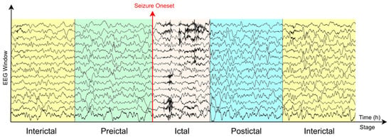
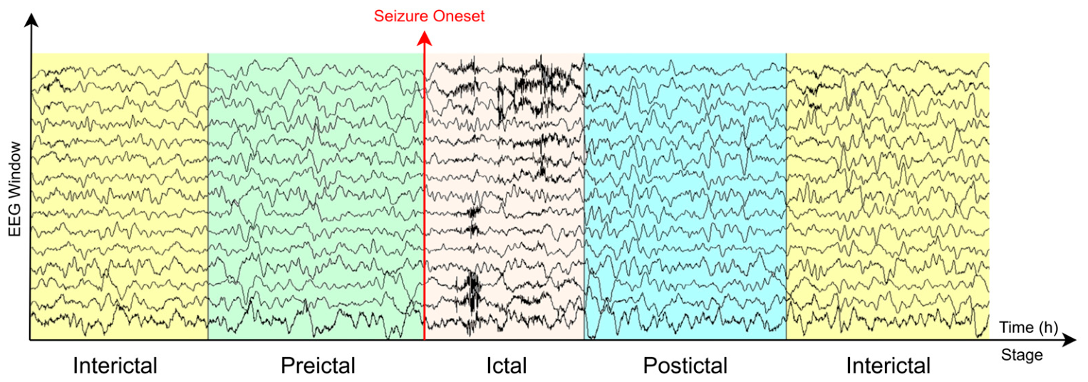
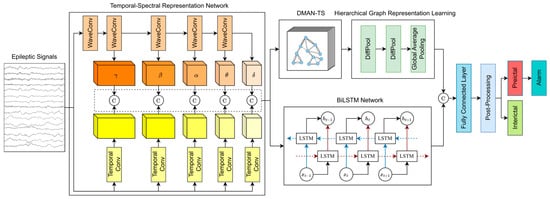
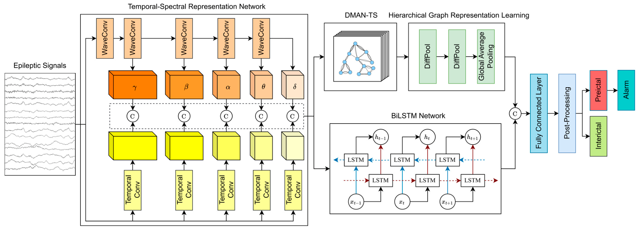
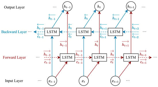
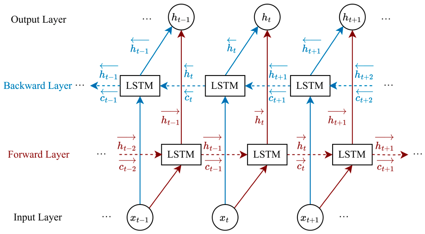
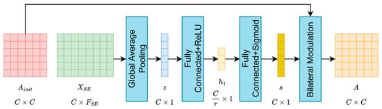
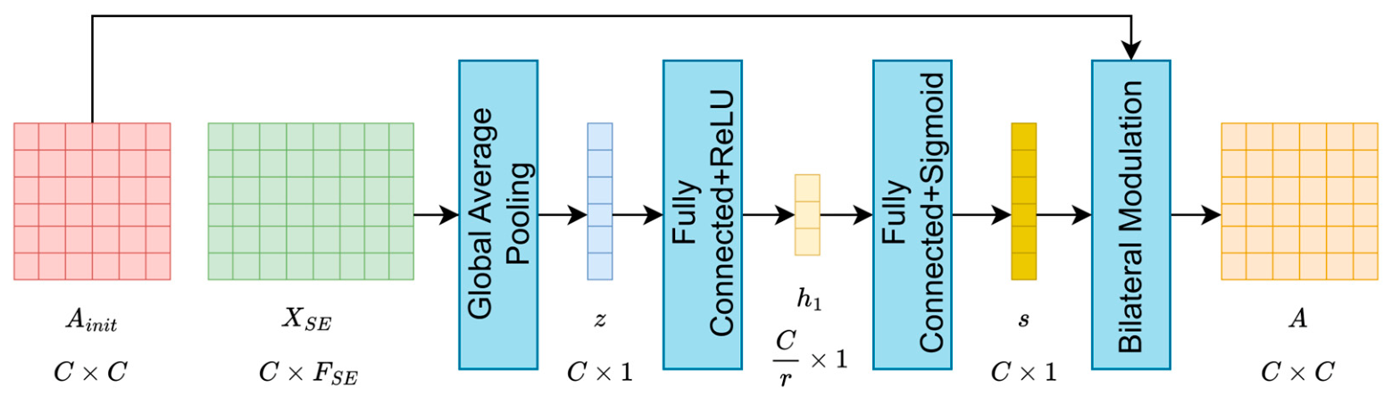
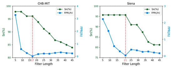
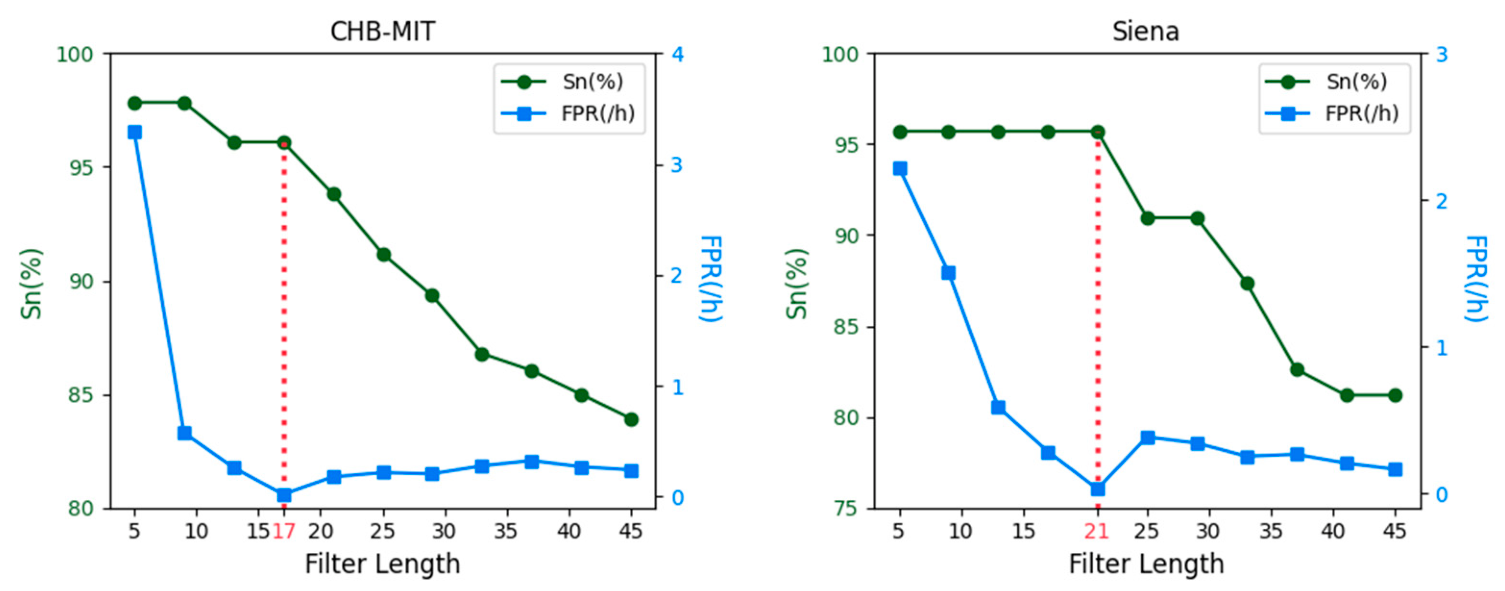
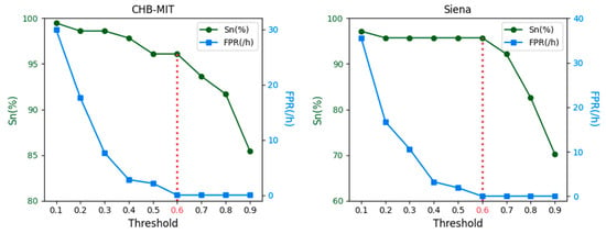
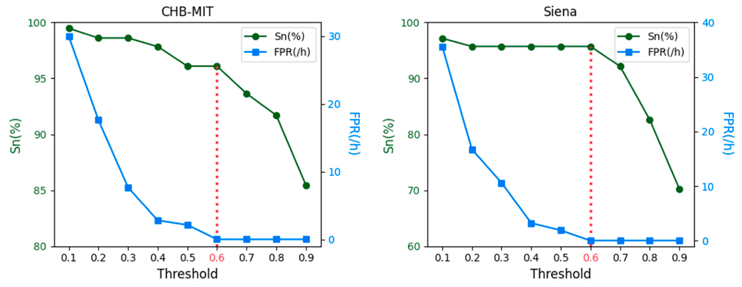
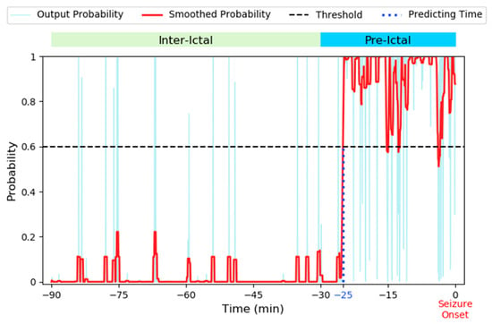
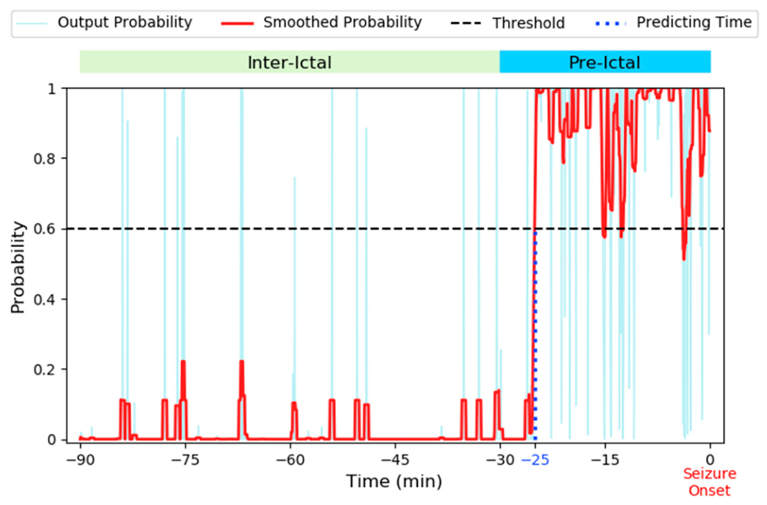
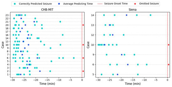
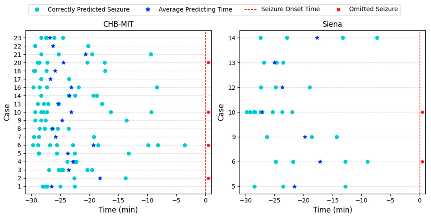
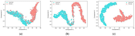
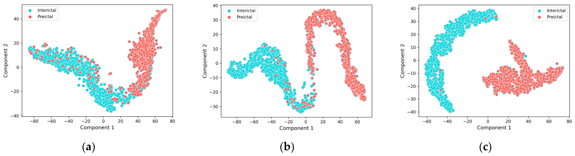

Disclaimer/Publisher’s Note: The statements, opinions and data contained in all publications are solely those of the individual author(s) and contributor(s) and not of MDPI and/or the editor(s). MDPI and/or the editor(s) disclaim responsibility for any injury to people or property resulting from any ideas, methods, instructions or products referred to in the content. |
© 2026 by the authors. Licensee MDPI, Basel, Switzerland. This article is an open access article distributed under the terms and conditions of the Creative Commons Attribution (CC BY) license.