


Abstract
Background/Objectives: Surrounding stimuli affect the visual processing of a target; however, whether this effect varies across stimulus types when peripheral targets do not need to be actively discriminated remains unclear. Methods: We recorded EEG activity from 20 participants during a central color judgment task while they viewed peripheral Gabor patterns, vertical stripes, letters, and numbers that were irrelevant to the task. Flankers appeared 1000 ms before targets in the flanked condition, providing an existing visual background. In the unflanked condition, only the fixation point was present before target onset. We compared event-related potentials (ERPs) and beta power between these conditions. Results: A spatiotemporal cluster permutation test revealed a significant interaction between stimulus type and flanker condition in the ERP results, with a cluster spanning 146–252 ms after target onset. Further comparisons revealed that flanker effects on ERP amplitude differed between Gabor patterns and vertical stripes. Within each stimulus condition, ERP changes were observed over different time ranges and scalp locations. Beta power was lower in the flanked condition for Gabor patterns, vertical stripes, and numbers, but no significant interaction was detected for beta power. Central color judgment responses were faster in the flanked condition, whereas accuracy did not differ significantly between conditions. Conclusions: These findings suggest that an existing flanker background can affect EEG responses after target onset without active discrimination of peripheral targets. Differences in flanker effects across stimulus types were supported by the ERP results, while beta power provided additional evidence of changes within stimulus conditions.
1. Introduction
Objects in everyday visual environments rarely appear in isolation. The presence and spatial arrangement of surrounding stimuli affect how we visually process a target. Previous research has shown that the distance between a Gabor pattern target and its flankers affects target detection performance [1]. The feature and spatial relationships between a central stimulus and surrounding stimuli can also change the apparent contrast of the target [2]. In addition to the distance between the target and flankers, the overall arrangement and grouping of surrounding stimuli also affect target discrimination performance [3,4,5]. Reviews of visual crowding also describe how surrounding stimuli can limit peripheral target recognition [6,7]. The effects of surrounding stimuli can also be observed in electrophysiological recordings. For example, surrounding gratings reduce the amplitude of steady-state visual evoked potentials elicited by a central grating [8]. The later N1 response is also more strongly suppressed when the surrounding gratings are parallel to the central grating than when they are perpendicular [9]. These findings indicate that visual responses after target onset depend not only on the target itself but also on the surrounding stimuli and their spatial arrangement.
In addition to spatial arrangement, stimulus type may also influence flanker effects. Grainger et al. [10] compared letters and symbols and reported greater interference from flankers for symbols. The two stimulus types also differed in their responses to flankers presented on one side or both sides of the target. Similar differences have been observed in string recognition. Position effects differ among letters, numbers, and other symbols, and the specific pattern also depends on the experimental conditions [11]. In peripheral vision, the effect of stimulus type on recognition performance also varies with target position and differs between the left and right visual fields [12]. These studies indicate that stimulus type is a factor to consider when examining visual interference. In a study of visual cues, Appelbaum et al. [13] compared the effects of orientation and phase cues on figure-ground segregation. They reported that neural responses differed between the cue conditions at a later stage. This finding suggests that differences in visual input may also be reflected in later neural responses, providing a basis for further comparisons of flanker effects across stimulus conditions.
Neural responses to visual stimuli also depend on the task participants are performing. Volberg and Greenlee [14] reported differences in neural responses between contour and noncontour stimuli during a contour detection task. The same differences were not observed during a central task. Increasing the central task load reduced the early C1 response to irrelevant stimuli in the upper visual field. The same effect was not observed at corresponding locations in the lower visual field [15]. These results indicate that neural responses to peripheral stimuli may vary with task demands. Even when the stimuli remain unchanged, their processing may be affected by the current task. In a study of texture segregation, task demands had different effects on the earlier N2 response and the later P3 response [16]. This suggests that task effects may be reflected in neural activity at different stages of processing.
In addition to event-related potentials (ERPs), power within specific frequency bands can be used to examine visual processing. Previous research has shown that the effects of visual attention on neural synchronization depend on frequency [17]. In a visual crowding task, a reduced N1 response was accompanied by a decrease in beta power. Changes in beta power are also related to target discrimination performance [18]. Potentials measured relative to event onset and oscillatory activity can capture different features of neural responses [19]. Therefore, beta power analysis can complement the analysis of flanker effects on ERP amplitude by examining whether changes are also present in frequency band activity.
Previous research has indicated that visual information may still elicit neural responses when it does not need to be actively discriminated. However, these responses are also affected by task demands. It remains to be tested whether flanker effects on ERP amplitude differ across peripheral stimulus types under the same central task demands. In this study, we used Gabor patterns, vertical stripes, letters, and numbers as peripheral targets and compared EEG activity between the flanked and unflanked conditions. The participants needed to judge only the color of the central fixation point. They did not need to report the orientation or identity of the peripheral targets. In the flanked condition, the flankers appeared before the target so that the target was presented within an existing visual background. We expected flankers to affect ERP amplitude after target onset even when peripheral targets did not need to be actively discriminated. These changes might differ across stimulus conditions. Our main test focused on the interaction between stimulus type and flanker condition in ERPs. We further examined the timing and scalp distribution of differences within each stimulus condition and used beta power analysis to examine additional changes in frequency band activity.
2. Materials and Methods
2.1. Participants
A total of 21 participants were recruited. One participant was excluded because of excessive noise in the EEG recordings, leaving 20 participants in the final sample. The final sample had a mean age of 21.35 years (SD = 0.75) and included 2 women and 18 men. A sensitivity analysis conducted in G*Power (version 3.1.9.7) indicated that, with 20 participants, a two-sided paired t test at α = 0.05 and 80% power was sensitive to an effect with a Cohen’s dz of approximately 0.66 or greater [20]. All participants had normal or corrected-to-normal vision and no history of neurological disorders. Written informed consent was obtained from all participants before the experiment. The study was approved by the Tsushima District Ethics Committee of Okayama University (protocol code Tsushima 24-009).
2.2. Apparatus and Stimuli
Visual stimuli were presented using MATLAB R2018a and Psychtoolbox-3 (version 3.0.19.11) on a Cambridge Research Systems Display++ monitor (Cambridge Research Systems Ltd., Rochester, UK) with a screen resolution of 1920 × 1080 pixels. Participants viewed the screen from 70 cm against a neutral gray background (RGB = [128, 128, 128]). Four types of peripheral stimuli were used, including Gabor patterns, vertical stripes, letters, and numbers. Each stimulus type retained its own visual features, and luminance and contrast were not matched across types.
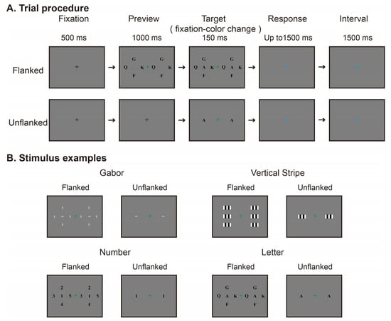
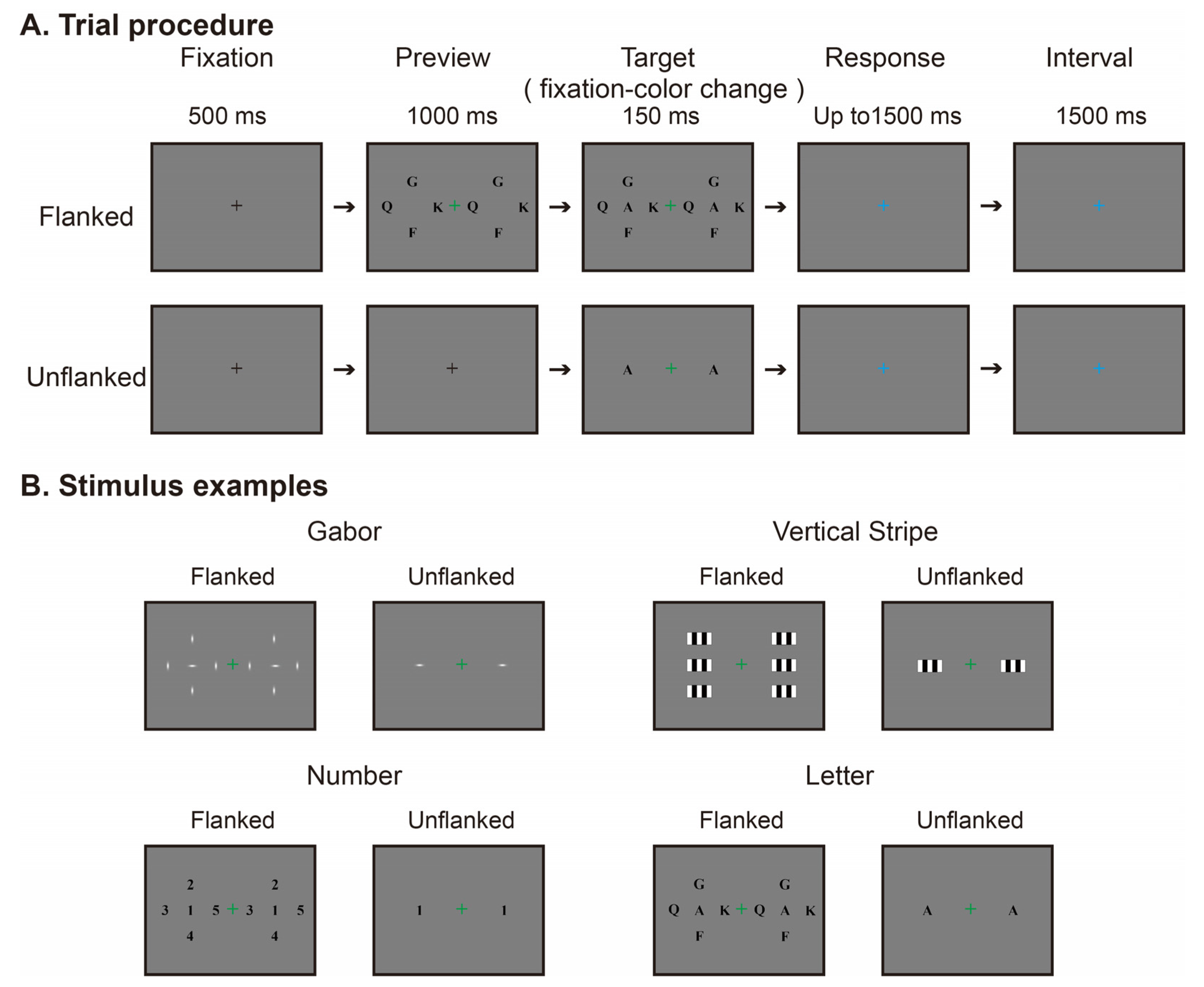
The Gabor pattern stimuli were generated by multiplying a sinusoidal grating by a two-dimensional Gaussian envelope. The image size was 70 × 70 pixels, corresponding to approximately 2.08° × 2.08° of visual angle. The sinusoidal carrier had a spatial frequency of approximately 0.72 cycles per degree, a phase of −90°, and a contrast parameter of 1. The Gabor pattern orientations were 0°, 45°, 90°, or 135°. For the Gaussian envelope, the standard deviations along the two orthogonal axes were approximately 0.12° and 0.35°, respectively. The vertical stripes stimulus consisted of alternating black and white vertical rectangular stripes, with five bands of equal width and white bands at both edges. The stimulus size was 140 × 70 pixels, corresponding to approximately 4.17° × 2.08° of visual angle. Each band was 28 pixels wide, corresponding to approximately 0.83° of visual angle. The same pattern was used for the target and flankers. No additional phase shift was applied. The letters stimuli consisted of A, F, G, K, Q, T, U, W, and Z, presented in black, bold Times New Roman font at a size of 70 × 70 pixels, corresponding to approximately 2.08° × 2.08° of visual angle. The numbers stimuli consisted of 1, 2, 3, 4, 5, and 7, with the same font, color, and size as the letter stimuli. For letters and numbers, the target and the four flankers were all different characters within each trial. The letter and number sets were selected by visual inspection to avoid including easily confused pairs, such as O and Q, M and W, and 6 and 9. No numerical similarity threshold was used. The stimulus examples are shown in Figure 1.
Figure 1.
Experimental procedure and stimulus examples. (A) Trial procedure in the flanked and unflanked conditions, illustrated with letters stimuli. The duration of each stage is shown in the figure. In the flanked condition, the flankers appeared before the targets and disappeared at the same time as the targets. At target onset, the central fixation point turned red or green. The green color is shown in the figure. The fixation point then turned blue, signaling the start of the response period, during which participants reported its preceding color (red or green). The blue fixation point remained visible until the next trial began with a black fixation point. The participants judged only the color of the fixation point and did not need to discriminate the peripheral targets. (B) Examples of the four peripheral stimulus types in the two flanker conditions. Identical target and flanker configurations were presented simultaneously in the left and right visual fields. The target center eccentricity was 9°, and the distance between the center of the target and each adjacent flanker was 4.5°.
2.3. Experimental Design
The main experiment used a within-subject design with four stimulus types—Gabor patterns, vertical stripes, letters, and numbers—and two flanker conditions, unflanked and flanked. The condition without flankers was labeled as unflanked, and the condition with flankers was labeled as flanked. Peripheral stimuli were presented simultaneously to the left and right of the central fixation point. The target identity and flanker arrangement were identical in the left and right visual fields within each trial. The target centers were located at an eccentricity of 9° to the left and right of the central fixation point. Only the targets were presented in the unflanked condition. In the flanked condition, the flankers surrounded each target, with a distance of 4.5° between the target center and each flanker center. For each stimulus type, the target size was the same in both conditions. For Gabor patterns, letters, and numbers, four flankers were placed above, below, to the left, and to the right of each target. For vertical stripes, two flankers were placed above and below each target. Through the visual angle conversion in the program, the approximate horizontal distance from the fixation point to the inner edge of the target image was found to be 7.96° for the Gabor patterns, letters, and numbers and 6.92° for the vertical stripes. In the flanked condition, the inner edge of the flanker image closest to the fixation point was approximately 3.46° from the fixation point for the Gabor patterns, letters, and numbers. For vertical stripes, the flankers were aligned vertically with the target so that their inner edges were the same horizontal distance from the fixation point as the target. These distances refer to the displayed image boundaries. The stimulus arrangements are shown in Figure 1.
The spatial parameters of the main experiment were selected on the basis of a separate behavioral pilot experiment with nine participants. The pilot experiment used Gabor patterns, letters, and numbers. We varied the target eccentricity at 9°, 11°, and 13° and the distance between the target and flanker centers at 2.5°, 3.5°, and 4.5°. The target and flankers appeared simultaneously in either the left or right visual field, with the side selected randomly. Participants reported the orientation of the Gabor patterns or the identity of the letter or number by selecting a response with the mouse. Repeated-measures ANOVAs revealed significant main effects of eccentricity and spacing for all three stimulus types (ps ≤ 0.010). None of the interactions were significant (ps ≥ 0.119). At an eccentricity of 9° and a spacing of 4.5°, the accuracy was 93.33% for Gabor patterns, 92.50% for letters, and 90.56% for numbers. We therefore used this spatial arrangement in the main experiment because it yielded relatively good discrimination performance. Vertical stripes were not included in the pilot experiment. The same spatial parameters were used for the vertical stripes in the main experiment.
2.4. Experimental Procedure
The central color judgment task was used to encourage participants to maintain their fixation at the center of the screen and to minimize active observation of the peripheral stimuli. The peripheral stimuli were irrelevant to the task, and participants were not required to discriminate or report their orientation or identities. Each trial began with a black central fixation point presented for 500 ms, followed by a 1000 ms preview period. In the flanked condition, the flankers were presented together with the central fixation point. In the unflanked condition, only the central fixation point was presented during the preview period. This arrangement allowed us to compare EEG responses after target onset in two different visual backgrounds and examine the flanker effect as a context effect. Following the preview period, the peripheral targets were presented for 150 ms. At target onset, the central fixation point simultaneously changed from black to either red or green. After 150 ms, both the targets and the flankers disappeared, and the central fixation point changed to blue. Participants were instructed to report the preceding color of the fixation point by pressing the F key for green and the J key for red. The response window lasted up to 1500 ms after the target offset. The reaction time was measured from the target offset. After a response was made or after the 1500 ms response window had elapsed, the blue fixation point remained on the screen for an additional 1500 ms. No accuracy feedback was provided during the experiment. The trial procedure is shown in Figure 1.
Each stimulus type was presented in a separate block, which resulted in four experimental blocks. The order of the four stimulus type blocks was counterbalanced across participants using a cyclic Latin square with four sequences. An additional check of the mean flanked minus unflanked difference within the main ERP interaction cluster revealed no significant effect of block position (χ2(3) = 4.12, p = 0.248) or presentation sequence (χ2(3) = 0.57, p = 0.903). Within each block, the unflanked and flanked trials were randomly intermixed. Each stimulus type was presented under both the unflanked and flanked conditions, with 60 trials in each condition. This resulted in 480 experimental trials for each participant. Each block lasted approximately 7.5 min. Participants could rest between blocks as needed, and a fixed break of 5 min was scheduled after the first two blocks. The main experimental blocks and the fixed break took approximately 35 min in total. The actual duration varied depending on the number of additional breaks. Before the formal experiment, participants completed practice trials to familiarize themselves with the task and response procedure.
2.5. EEG Recording and Processing
EEGs were recorded continuously using active Ag/AgCl electrodes (actiCAP snap, Brain Products GmbH, Gilching, Germany) mounted on an elastic cap (CACS-64-SAMW, Easycap GmbH, Wörthsee, Germany). Scalp electrodes were positioned according to the standard 10-10 system. A BrainAmp DC amplifier (Brain Products GmbH, Gilching, Germany) was used. The recordings included 29 scalp channels, one horizontal electrooculogram (HEOG) channel, and one vertical electrooculogram (VEOG) channel. The left earlobe served as the online reference, and AFz served as the ground electrode. Electrode impedances were maintained below 5 kΩ, and the sampling rate was 500 Hz. EEG preprocessing was performed using EEGLAB 2025.0.0 in MATLAB R2024b [21]. Continuous data were bandpass filtered from 0.1 to 80 Hz and notch filtered from 49 to 51 Hz. After the segments containing obvious nonphysiological noise were removed, the data were re-referenced to the average of the scalp electrodes. Extended Infomax independent component analysis (ICA) was performed on the continuous data from the 29 scalp channels using the runica algorithm [22]. Components reflecting eye movements or other clear artifacts were manually identified and removed. This assessment used ICLabel classifications [23], component time courses and scalp distributions, and their relationships with HEOG and VEOG activity. An average of 5.15 ± 1.53 independent components were removed per participant (mean ± SD). HEOG and VEOG were used only to help identify components related to eye movements and were not included in subsequent analyses.
After ICA cleaning, the data for ERP analysis were further lowpass filtered at 30 Hz and divided into epochs from −200 to 500 ms relative to peripheral target onset. Trials were rejected if the amplitude exceeded ±100 μV at any scalp EEG channel within this time window. Baseline correction was then applied to each channel using the interval from −200 to 0 ms. Trials with both correct and incorrect responses in the central color judgment task were included in the ERP analysis. After artifact rejection, the numbers of retained trials in the unflanked and flanked conditions were 58.45 ± 2.65 and 58.00 ± 3.46 for Gabor patterns, respectively. The corresponding values were 57.75 ± 2.90 and 57.75 ± 3.54 for vertical stripes, 57.80 ± 3.25 and 57.50 ± 3.44 for letters, and 58.20 ± 2.69 and 57.95 ± 3.25 for numbers (mean ± SD), respectively. The overall number of retained trials did not differ significantly between the two flanker conditions (t(19) = −0.96, p = 0.350).
To examine changes in potential before target onset, we also prepared ERP data over a longer time interval without baseline correction. After ICA cleaning, the data were lowpass filtered at 30 Hz and divided into epochs from −1500 to 500 ms relative to target onset. Artifact rejection used a threshold of ±100 μV across the entire epoch. This interval covered the initial fixation period, the preview period, and activity after target onset. The mean number of retained trials ranged from 56.90 to 57.65 across conditions. The overall number did not differ significantly between the two flanker conditions (t(19) = 0.22, p = 0.831).
Time–frequency decomposition was performed using complex Morlet wavelets over 8–30 Hz in steps of 1 Hz. The number of wavelet cycles increased linearly from 4 at 8 Hz to 10 at 30 Hz. Power was normalized to the initial fixation period from −1500 to −1250 ms and converted to decibels using 10 log10(P/Pbaseline). Previous research has linked changes in beta power to target discrimination performance in a visual crowding task [18]. We therefore used beta power as a measure to complement ERPs, averaging normalized power over 13–30 Hz and analyzing activity from 0 to 500 ms after target onset. The mean number of retained trials ranged from 55.35 to 57.10 across conditions. The overall number did not differ significantly between the two flanker conditions (t(19) = 0.25, p = 0.807).
Subsequent ERP and time–frequency statistical analyses used 27 scalp electrodes, including F7, F3, Fz, F4, F8, FC5, FC1, FCz, FC2, FC6, T7, C3, Cz, C4, T8, CP5, CP1, CP2, CP6, P7, P3, Pz, P4, P8, O1, Oz, and O2. Fp1 and Fp2 were excluded from the spatiotemporal statistical analyses because they are susceptible to residual eye movement activity.
2.6. Statistical Analysis
Statistical analyses were performed using R 4.2.3 and MATLAB R2024b. The significance level was set at α = 0.05. Condition differences in ERP amplitude and beta power were both defined as flanked minus unflanked. The behavioral measures included accuracy and reaction time in the central color judgment task. The accuracy was calculated from all valid trials. The reaction time analyses included only correct trials. For each participant, stimulus type, and flanker condition, trials with reaction times more than 2.5 SDs above or below the condition mean were excluded. Separate repeated-measures ANOVAs were performed on accuracy and reaction time, with four stimulus types and two flanker conditions. The Greenhouse–Geisser correction was applied to effects that did not meet the sphericity assumption. Partial eta squared (ηp2) was reported as the effect size.
ERP data were analyzed using spatiotemporal cluster permutation tests in R 4.2.3 [24]. The analysis covered 27 electrodes from 0 to 500 ms after target onset, with a time step of 2 ms. Spatial neighbors were defined in advance on the basis of the relative positions of the electrodes on the scalp. Adjacent time samples were 2 ms apart. Samples at electrode and time combinations that met the cluster formation threshold and were adjacent in space or time were grouped into the same cluster. We first tested the interaction between stimulus type and flanker condition. For each participant, we calculated the flanked minus unflanked difference for each of the four stimulus types. An F test with four levels of stimulus type and repeated measures was performed at each electrode and time point. The cluster formation threshold was set at α = 0.05 for each sample. The cluster statistic was the sum of the F values within the cluster. A null distribution was constructed from 5000 permutations of stimulus labels within each participant. Each permutation retained the maximum cluster statistic across all electrodes and time points. Clusters with p < 0.05 were considered significant. For each significant interaction cluster, we calculated the mean difference for each participant and stimulus type using only the samples belonging to that cluster. We then performed six paired t tests with Holm correction and reported the mean differences, 95% confidence intervals, and Cohen’s dz.
We then tested flanker effects within each stimulus type. A paired t statistic was calculated at each electrode and time point. The cluster formation threshold was set at α = 0.05 for a two-sided test at each sample. Adjacent samples above the threshold were grouped separately into positive and negative clusters. The cluster statistic was the sum of absolute t values within the cluster. We performed 5000 sign-flip permutations among the participants. In each permutation, the same sign was applied to a participant’s differences across all four stimulus types, electrodes, and time points. The maximum cluster statistic across all four stimulus types and both positive and negative clusters was retained to construct a common null distribution for multiple comparison correction. Clusters with a corrected p < 0.05 were considered significant. The time ranges and electrode distributions of clusters were used only to describe the detected differences. They were not used to determine the exact onset or offset of an effect or significance in individual samples.
Potentials before target onset were examined using ERP data over a longer time interval without baseline correction. Changes in potential during the preview period were shown at Fz, Cz, Pz, and Oz. We tested the overall mean offset in potential differences from −200 to 0 ms. For each participant and stimulus type, signed flanked minus unflanked differences were averaged across this time window and the 27 electrodes. A one-sample t test was then used to test whether the mean differed from zero. We also tested the difference averaged across the four stimulus types within each participant. This analysis reflects the overall mean offset and does not rule out local differences. We also performed exploratory spatiotemporal cluster permutation tests over the same time window, using the cluster formation threshold, neighbor definitions, and cluster statistic from the ERP analysis. For each stimulus type, 5000 sign-flip permutations were performed, retaining the maximum cluster statistic across positive and negative clusters. No additional multiple comparison correction was applied across the four stimulus types.
Beta power analyses were restricted to 13–30 Hz, 0–500 ms after target onset, and the 27 electrodes. Spatial neighbors were defined using a predefined electrode neighbor list. Temporal neighbors were consecutive time points in the data used for the time–frequency statistical analyses. Flanker effects within each stimulus type were tested using the same two-sided t statistic, cluster formation threshold, and cluster statistic as in the ERP analysis. We performed 5000 sign-flip permutations and retained the maximum cluster statistic across all four stimulus types, electrodes, time points, and both positive and negative clusters. We reported cluster p values corrected across the four stimulus types within the beta band. Clusters with p < 0.05 were considered significant. We further tested the interaction between stimulus type and flanker condition using an F test with repeated measures and 5000 permutations of stimulus labels within each participant. The cluster formation threshold was set at α = 0.05 for each sample, and the cluster statistic was the sum of the F values within the cluster. Each permutation retained the maximum cluster statistic. Clusters with p < 0.05 were considered significant.
3. Results
3.1. Behavioral Results
For accuracy, the 4 (stimulus type) × 2 (flanker condition) repeated-measures ANOVA revealed no significant main effect of stimulus type (F(1.97, 37.50) = 1.16, p = 0.324, ηp2 = 0.058, Greenhouse–Geisser ε = 0.658), no significant main effect of flanker condition (F(1, 19) = 2.40, p = 0.138, ηp2 = 0.112), and no significant stimulus type × flanker condition interaction (F(2.59, 49.20) = 1.29, p = 0.287, ηp2 = 0.064, Greenhouse–Geisser ε = 0.863) (see Table 1).
Table 1.
Behavioral performance across stimulus types and flanker conditions.
For reaction time, there was a significant main effect of the flanker condition (F(1, 19) = 21.59, p < 0.001, ηp2 = 0.532), with faster responses in the flanked condition than in the unflanked condition. The main effect of stimulus type was not significant (F(2.35, 44.71) = 1.35, p = 0.271, ηp2 = 0.066, Greenhouse–Geisser ε = 0.784), and the stimulus type × flanker condition interaction was also not significant (F(2.11, 40.07) = 0.19, p = 0.835, ηp2 = 0.010, Greenhouse–Geisser ε = 0.703) (see Table 1).
3.2. ERP Results Relative to Target Onset
3.2.1. Interaction Between Stimulus Type and Flanker Condition
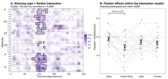
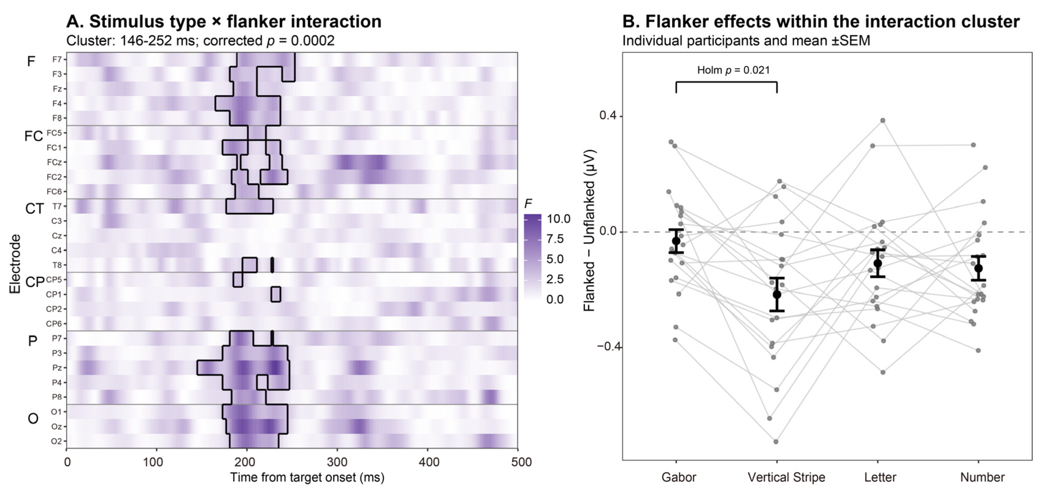
The spatiotemporal cluster permutation test revealed a significant interaction between stimulus type and flanker condition, with a cluster spanning 146–252 ms (cluster statistic ΣF = 2422.53, pcluster = 0.0002). The cluster involved 22 electrodes, including F7, F3, Fz, F4, F8, FC5, FC1, FCz, FC2, FC6, T7, T8, CP5, CP1, P7, P3, Pz, P4, P8, O1, Oz, and O2. Within the cluster, the mean flanked minus unflanked differences were −0.031 μV for Gabor patterns, −0.216 μV for vertical stripes, −0.108 μV for letters, and −0.125 μV for numbers. After Holm correction for the six pairwise comparisons, only the difference between Gabor patterns and vertical stripes was significant. The mean difference was 0.185 μV (95% CI [0.069, 0.302], t(19) = 3.34, corrected p = 0.021, dz = 0.75). None of the remaining comparisons were significant (see Figure 2).
Figure 2.
ERP interaction between stimulus type and flanker condition. (A) Spatiotemporal distribution of F values for the interaction. Black outlines mark the samples belonging to the significant cluster, which spans 146–252 ms (corrected pcluster = 0.0002). Color indicates the magnitude of F values. Electrodes are grouped by scalp location. F, FC, CT, CP, P, and O indicate frontal, frontocentral, central and temporal, centroparietal, parietal, and occipital sites, respectively. (B) Mean flanked minus unflanked potential differences for each stimulus condition, calculated using the samples belonging to the significant cluster. Gray points and connecting lines represent data from individual participants. Black points and error bars show the mean across participants ± SEM. The horizontal dashed line indicates a difference of zero. After Holm correction for the six pairwise comparisons, only the difference between Gabor patterns and vertical stripes was significant (p = 0.021).
3.2.2. Flanker Effects on ERPs Within Each Stimulus Type
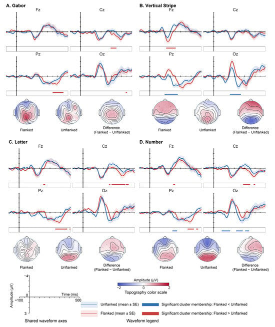
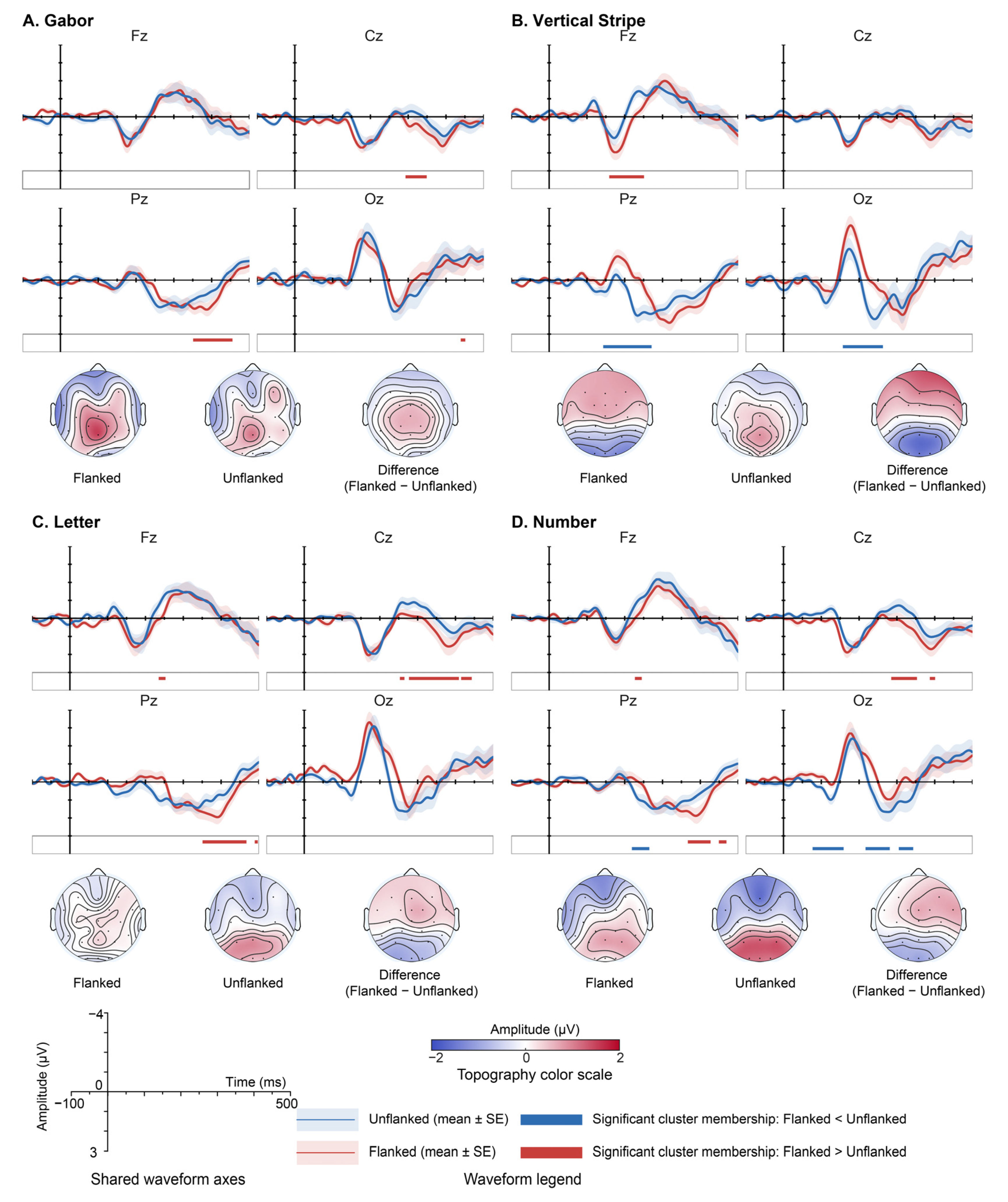
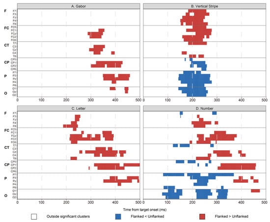
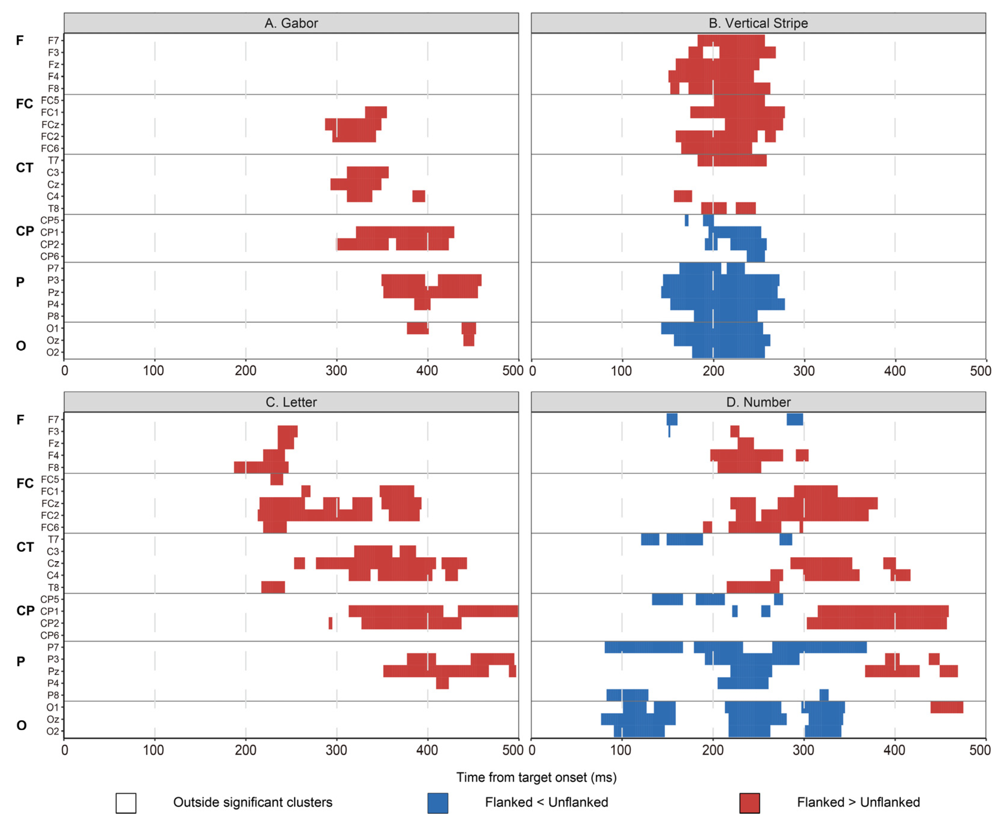
All p values below were corrected using the maximum cluster statistic across the four stimulus types, all electrodes and time points, and both positive and negative directions. The mean differences are reported as the mean ± SEM. Representative ERP waveforms and scalp distributions are shown in Figure 3. The full distributions of significant clusters across electrodes and time are shown in Figure 4.
Figure 3.
ERP waveforms and scalp topographies for the flanked and unflanked conditions across the four stimulus types. (A) Gabor patterns, (B) vertical stripes, (C) letters, and (D) numbers. Grand average ERP waveforms are shown at the representative electrodes Fz, Cz, Pz, and Oz from −100 to 500 ms. The blue and red traces indicate the unflanked and flanked conditions, respectively, with shaded areas representing ±SEM across participants. The negative voltage is plotted upward. Horizontal colored bars mark samples at each electrode and time point belonging to significant whole-scalp spatiotemporal clusters identified by the cluster-based permutation analysis after correction across the four stimulus types, all electrodes and time points, and both positive and negative directions. Red indicates flanked > unflanked and blue indicates flanked < unflanked. These bars are shown only as a visual reference to the whole-scalp cluster results and should not be interpreted as separate significance tests at individual electrodes. Scalp voltage distributions are shown for the flanked condition, the unflanked condition, and their difference (flanked − unflanked) over representative time windows for each stimulus type. These windows are 302–402 ms for Gabor patterns, 160–260 ms for vertical stripes, 198–298 ms for letters, and 220–320 ms for numbers and were selected within the time ranges covered by significant clusters to illustrate representative scalp distributions. All scalp maps use the same symmetric scale (−2 to 2 μV), with electrode locations indicated by black dots. Shared waveform axes and legends apply to all panels.
Figure 4.
Whole-scalp spatiotemporal cluster-based permutation results for the flanked versus unflanked comparison across the four stimulus types. (A) Gabor patterns, (B) vertical stripes, (C) letters, and (D) numbers. Each panel shows the distribution across electrodes and the time of significant spatiotemporal clusters from 0 to 500 ms after target onset across the 27 scalp electrodes included in the whole-scalp analysis. The colored cells indicate samples at each electrode and time point belonging to significant clusters identified by the cluster-based permutation test. Differences in cluster time ranges and scalp distributions across stimulus types are descriptive. Statistical comparisons between stimulus types are reported separately in Figure 2. Correction used the maximum cluster statistic across all four stimulus types, all electrodes and time points, and both positive and negative directions. Red indicates flanked > unflanked, whereas blue indicates flanked < unflanked. White cells indicate samples not belonging to a significant cluster. Colored samples represent cluster membership at the cluster level and should not be interpreted as independently significant effects at individual electrodes and time points. Electrodes are arranged approximately from anterior to posterior and grouped for visualization as F (frontal), FC (frontocentral), CT (central and temporal), CP (centroparietal), P (parietal), and O (occipital), with horizontal lines separating the groups.
For Gabor pattern stimuli, one significant spatiotemporal cluster was observed from 288 to 458 ms after target onset (cluster statistic Σ|t| = 1080.96, pcluster = 0.0104). It was a positive cluster with a mean difference of 0.569 ± 0.078 μV. The cluster involved FC1, FCz, FC2, C3, Cz, C4, CP1, CP2, P3, Pz, P4, O1, and Oz.
For the vertical stripes stimuli, two significant spatiotemporal clusters were identified. The positive cluster spanned 152–278 ms, with a mean difference of 0.879 ± 0.112 μV (cluster statistic Σ|t| = 1667.32, pcluster = 0.0014). It involved F7, F3, Fz, F4, F8, FC5, FC1, FCz, FC2, FC6, T7, C4, and T8. The negative cluster spanned 144–278 ms, with a mean difference of −1.151 ± 0.177 μV (cluster statistic Σ|t| = 1705.48, pcluster = 0.0010). It involved CP5, CP1, CP2, CP6, P7, P3, Pz, P4, P8, O1, Oz, and O2.
For the letters stimuli, a significant positive cluster spanned 188–500 ms, with a mean difference of 0.700 ± 0.107 μV (cluster statistic Σ|t| = 1992.10, pcluster = 0.0004). It involved F3, Fz, F4, F8, FC5, FC1, FCz, FC2, FC6, C3, Cz, C4, T8, CP1, CP2, P3, Pz, and P4.
For the numbers stimuli, one positive cluster and one negative cluster were identified. The positive cluster spanned 190–474 ms, with a mean difference of 0.769 ± 0.094 μV (cluster statistic Σ|t| = 1958.93, pcluster = 0.0004). It involved F3, Fz, F4, F8, FC1, FCz, FC2, FC6, Cz, C4, T8, CP1, CP2, P3, Pz, and O1. The negative cluster spanned 78–368 ms, with a mean difference of −0.837 ± 0.097 μV (cluster statistic Σ|t| = 1841.96, pcluster = 0.0006). It involved F7, F3, T7, CP5, CP1, P7, P3, Pz, P4, P8, O1, Oz, and O2.
3.3. Activity Before Target Onset and Baseline Checks
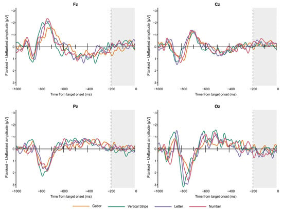
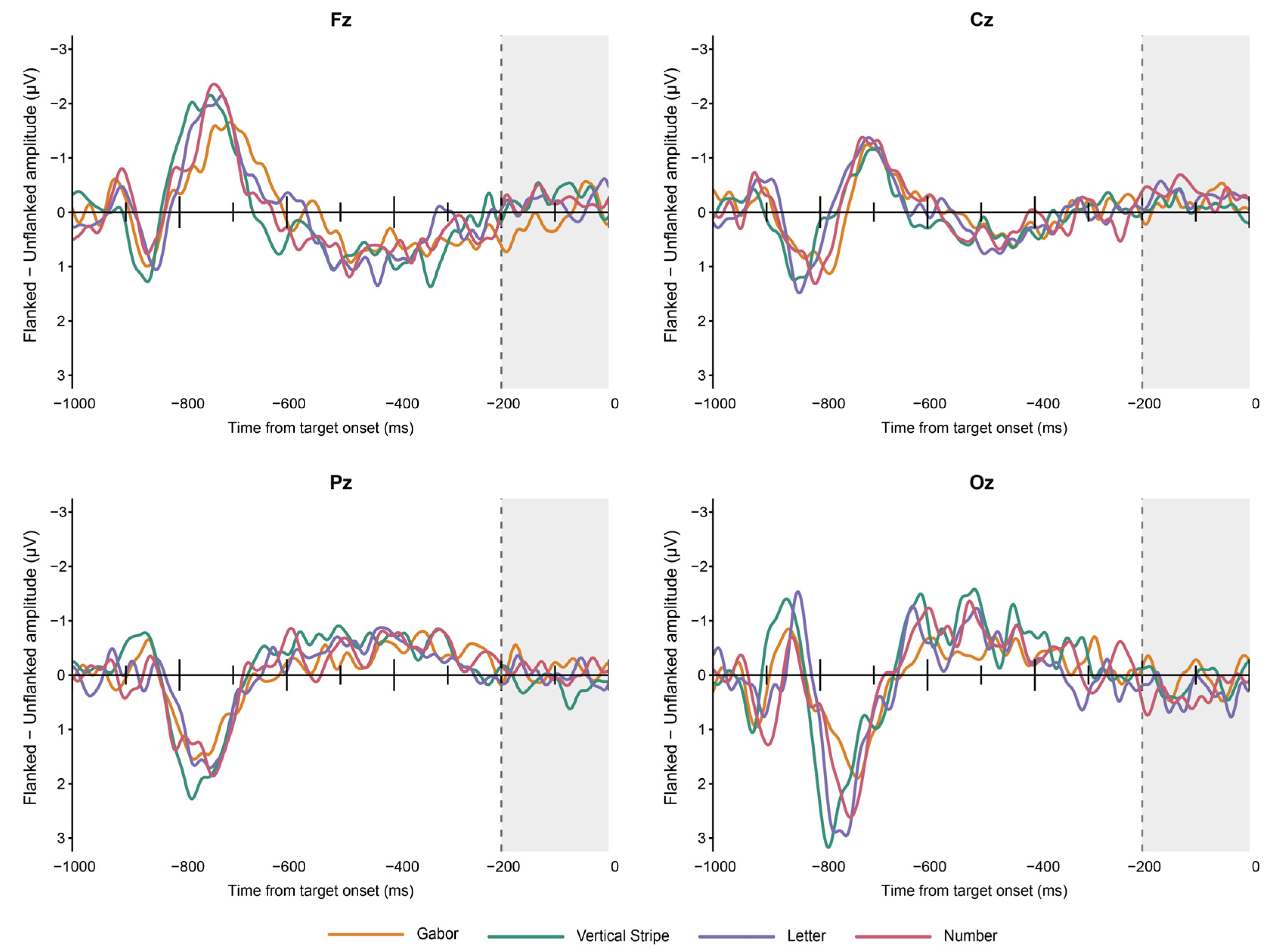
Flanked minus unflanked difference waveforms before target onset, without baseline correction, are shown in Figure 5.
Figure 5.
ERP difference waveforms before target onset. Mean flanked minus unflanked potential differences across the 20 participants are shown at Fz, Cz, Pz, and Oz from −1000 to 0 ms without baseline correction. The preview period begins at −1000 ms, and the target onset is at 0 ms. The gray area indicates the baseline interval from −200 to 0 ms used in the main ERP analysis. The vertical dashed line indicates the start of this interval. The negative voltage is plotted upward.
Exploratory spatiotemporal cluster tests over the baseline interval from −200 to 0 ms identified six local clusters of condition differences. There was one negative cluster each for Gabor patterns and letters, two positive clusters for vertical stripes, and one positive and one negative cluster for numbers. All six clusters were significant after correction using the maximum cluster statistic within each stimulus type (ps < 0.05). No additional correction was applied across stimulus types. After averaging the signed potential differences across this time window and the 27 electrodes, the mean differences were −0.001 μV for Gabor patterns, 0.019 μV for vertical stripes, −0.001 μV for letters, and 0.016 μV for numbers. None differed significantly from zero, with t(19) = −0.28, p = 0.782 for Gabor patterns, t(19) = 1.78, p = 0.091 for vertical stripes, t(19) = −0.06, p = 0.953 for letters, and t(19) = 2.04, p = 0.056 for numbers. The difference averaged across the four stimulus types was 0.008 μV (t(19) = 1.32, p = 0.204).
3.4. Beta Power Results After Target Onset
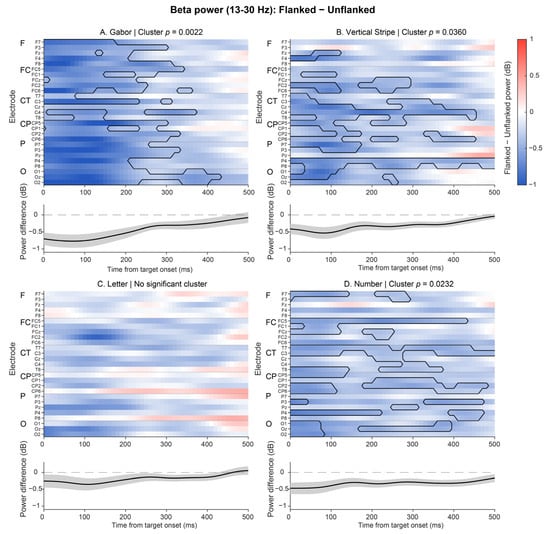
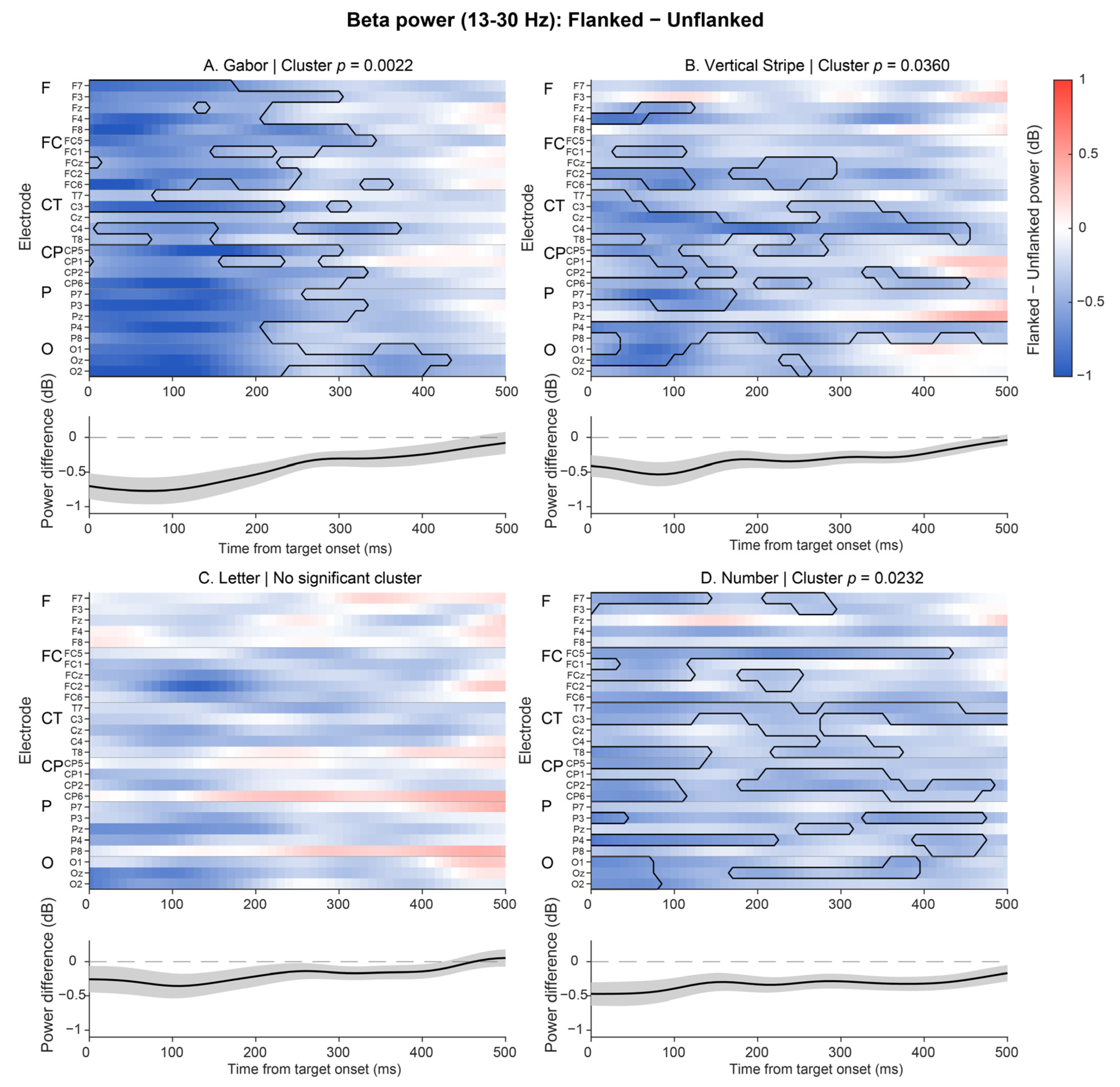
Within 13–30 Hz and 0–500 ms, cluster statistics were corrected using the maximum across the four stimulus types, all electrodes and time points, and both positive and negative directions within the beta band. Gabor patterns had a significant negative cluster in the flanked minus unflanked power difference from 0 to 430 ms, involving 26 electrodes (pcluster = 0.0022). Vertical stripes had a significant negative cluster from 0 to 500 ms, involving 22 electrodes (pcluster = 0.0360). Numbers had a significant negative cluster from 0 to 500 ms, involving 22 electrodes (pcluster = 0.0232). No significant cluster was detected for letters. The test of the interaction between stimulus type and flanker condition did not reveal a significant cluster. The results are shown in Figure 6.
Figure 6.
Flanker effects on beta power across the four stimulus types. (A) Gabor patterns, (B) vertical stripes, (C) letters, and (D) numbers. The plots show mean flanked minus unflanked beta power differences across the 20 participants from 0 to 500 ms after target onset. Power was averaged over 13–30 Hz and is expressed in decibels. Blue indicates lower power in the flanked condition, and red indicates higher power. All panels use the same color scale. Black outlines indicate the samples belonging to significant clusters. The p values shown were corrected using the maximum cluster statistic across all four stimulus types, all electrodes and time points, and both positive and negative directions within the beta band. No significant cluster was detected for letters. The black curve below each plot shows the power difference averaged first across the 27 electrodes and then across participants. The gray shading represents ±SEM, and the horizontal dashed line indicates a difference of zero. The curves describe the overall changes and do not represent separate significance tests. Electrode group abbreviations are the same as those in Figure 4.
4. Discussion
4.1. Overview of the Main Findings
In this study, flanker effects on EEG activity across peripheral stimulus conditions while participants performed a central color judgment task were examined. ERP analysis revealed an interaction between stimulus type and flanker condition. Further comparisons revealed that flanker effects on ERP amplitude differed significantly between Gabor patterns and vertical stripes. This finding indicates that flanker effects on ERP amplitude may vary with the type of visual input even when participants do not need to actively discriminate peripheral targets. Winsler et al. [25] compared letters and symbols in a peripheral character discrimination task and also found that flanker effects on ERPs differed between the two stimulus types. We observed similar differences across stimulus types during a central color judgment task. This provides additional evidence for understanding flanker effects on peripheral stimuli that are irrelevant to the task. Analyses within each stimulus condition also revealed flanker effects on ERPs across different time ranges and scalp locations. Beta power was lower in the flanked condition than in the unflanked condition for Gabor patterns, vertical stripes, and numbers. However, the interaction between stimulus type and flanker condition was not significant. Thus, the ERP results support differences in flanker effects across stimulus conditions, whereas the beta results reveal that flanker effects on power are also present in some stimulus conditions.
4.2. Spatiotemporal Features of Flanker Effects on ERPs
ERP analysis revealed an interaction between stimulus type and flanker condition, with a cluster spanning 146–252 ms after target onset. Further comparisons revealed that flanker effects differed significantly between Gabor patterns and vertical stripes. Previous research has also shown that the relationship between a target and its flankers affects visual responses after target onset. Schallmo et al. [9] reported that surrounding gratings reduced the earlier C1 response. Differences between orientation configurations were observed mainly in the N1 response at approximately 160 ms. Chicherov et al. [26] varied the length of flanking lines to change how the target and flankers grouped together. They reported that the related differences appeared mainly in the N1 response after 180 ms. These studies indicate that flanker effects may involve both early visual responses and later processing of the relationship between the target and flankers. Consistent with these findings, a negative cluster from 144 to 278 ms in the vertical stripes condition involved mainly parietal and occipital scalp sites. This change may be related to the feature relationships between the target and flankers or to visual grouping.
In the vertical stripes condition, positive changes at anterior sites and negative changes at posterior sites occurred over similar time ranges. This produced a scalp distribution with opposite polarities at anterior and posterior sites. Because the flankers appeared before the target, the target was presented within an existing flanker background. Its appearance changed the existing visual configuration. Joo et al. [27] and Joo and Murray [28] reported that flanker arrangement, stimulus spacing, and surface configuration affect the P1 response after target onset. These findings indicate that visual responses to a newly presented target are also related to the existing background. In light of these studies, the changes in ERP amplitude in our experiment may involve the integration or segregation of target and surrounding information after the target appears within the flanker background.
Changes in ERP amplitude also extended to later time periods in some stimulus conditions. The positive cluster in the Gabor patterns condition occurred from 288 to 458 ms. The positive clusters in the letters and numbers conditions extended to 500 and 474 ms, respectively. These clusters involved central scalp sites and some anterior and posterior sites. In a study of texture segmentation, Scholte et al. [29] reported that boundary detection and surface segregation followed different time courses. The responses after 200 ms also involved a wider range of scalp sites. This finding is consistent with the later changes in ERP amplitude observed in some conditions in our experiment. These changes may be related to further processing of the overall visual input after target onset. Flanker effects may therefore extend into the continued processing of the target and surrounding information.
4.3. Changes in Beta Power and Their Relationship with the ERP Results
Beta power was lower in the flanked condition than in the unflanked condition for Gabor patterns, vertical stripes, and numbers. In a letter crowding task, decreases in beta power were related to the degree of flanker interference and individual target discrimination performance [18]. Di Dona et al. [30] also examined the role of parietal beta activity in resolving visual crowding. Together, these findings suggest that beta activity may be related to interactions between peripheral targets and their surrounding flankers. More broadly, beta activity may help maintain the current sensorimotor or cognitive state [31]. Changes in beta activity may be related to adjustments in that state. In light of these findings, the decrease in beta power in some stimulus conditions in our experiment may be related to changes in visual processing or task preparation in the presence of flankers.
ERPs and beta power reflect different features of EEG activity and do not necessarily show the same pattern of change [19]. For example, Noonan et al. [32] reported that expected distraction reduced the P1 response without a corresponding change in alpha power. In our experiment, ERP differences were positive or negative at different scalp sites, whereas all significant beta effects showed decreases in power. The sign of an ERP difference indicates the direction of the potential difference between conditions. A difference in beta power indicates an increase or decrease in power within that frequency band. Therefore, the two measures do not need to change in the same direction. In addition, the ERP analysis revealed a significant interaction between stimulus type and flanker condition, whereas the beta power analysis did not detect this interaction. Specifically, the ERP results revealed that flanker effects differed significantly between Gabor patterns and vertical stripes. The beta analysis revealed decreases in power with flankers for Gabor patterns, vertical stripes, and numbers but revealed no significant effect of stimulus type on these flanker effects. Thus, both analyses revealed changes associated with flankers, but only the ERP results revealed that flanker effects varied across stimulus types.
4.4. Peripheral Visual Processing During a Central Task
The flankers were present for 1000 ms before target onset. The difference waveforms before target onset revealed that the larger voltage changes following flanker onset gradually leveled off as the target onset approached. In the baseline check, the condition differences averaged across the 27 electrodes and the entire time window did not differ significantly from zero for any stimulus type. However, brief local differences between conditions were still present. This suggests that the early voltage changes following flanker onset had decreased before target onset. Previous studies also revealed that flankers presented 1–2 s before a target could still affect the EEG response to that target [9,28]. In this study, participants only had to judge the color of the central fixation point. We still observed ERP changes related to flankers, and the flanker effect differed significantly between the Gabor patterns and vertical stripes conditions. This suggests that a continuously presented flanker background may still affect visual responses after target onset, even when peripheral targets do not need to be actively discriminated.
Previous studies of peripheral stimuli that were irrelevant to the task also provide evidence for this view. Crowded arrangements of peripheral letters have been associated with changes in visual cortical BOLD signals [33], whereas increasing central task load reduces visual cortical responses to irrelevant peripheral checkerboards [34]. The timing of these effects may also matter, as early occipital responses to texture segregation appear less sensitive to task demands than later responses do [35]. These findings are consistent with our results and indicate that the relationship between a peripheral target and its flankers may still affect visual processing even when the target is irrelevant to the current task. This effect may vary across stimulus types and stages of processing.
The behavioral results revealed shorter reaction times in the central color judgment task in the flanked condition but no significant change in accuracy. Because the flankers appeared 1000 ms before the central color change, they may have provided a cue about when the next event would occur, in addition to changing the peripheral visual input. Nobre and van Ede [36] reported that people can use regularities in event timing to adjust attention and response preparation. Participants may therefore have used the timing information provided by the earlier appearance of the flankers to prepare for the central color judgment, leading to shorter reaction times. Together with the ERP results, these findings suggest that flankers may affect both visual processing after target onset and preparation for the central task. These effects may be reflected in changes in ERP amplitude and shorter reaction times in the central task.
4.5. Limitations
Several aspects of the experimental design should be considered when interpreting the flanker effects in this study.
First, the flankers were already present before target onset. The visual background at target onset therefore differed between the flanked and unflanked conditions. Baseline checks revealed local, brief differences between conditions from −200 to 0 ms. However, the mean difference in potential between conditions, averaged across the entire time window and the 27 electrodes, did not differ significantly from zero. Because baseline correction was applied in the main ERP analysis, differences between conditions after target onset may still have been affected by background activity before target onset. In addition, the targets and flankers disappeared at the same time. Later changes in ERP amplitude may therefore include responses to stimulus offset. Future studies could separate the onset and offset times of targets and flankers to better distinguish these effects. A separate condition with flankers but no targets could also help distinguish ongoing background activity from responses following target onset.
The four stimulus types were not fully matched in size, contrast, spatial frequency, or the number and arrangement of flankers. The ERP interaction observed in this study therefore reflects differences between the specific stimulus conditions and cannot be attributed to a single stimulus property. Although the spatial arrangement was selected on the basis of the peripheral target discrimination performance in the pilot experiment, vertical stripes were not included. We therefore cannot confirm that the four stimulus types produced the same degree of crowding. The main experiment also did not require participants to report the peripheral targets. We therefore cannot determine how these neural changes are related to peripheral perceptual performance. Future studies could test this relationship by matching the main visual properties and including a peripheral discrimination task.
Participants were instructed to maintain a central fixation, but fixation position was not verified on each trial using an eye tracker. EOG recordings and ICA processing cannot fully replace eye tracking. Targets were presented simultaneously in both visual fields; therefore, this design could not separate the contributions of the left and right visual fields. The current results mainly describe the time course and scalp distribution of flanker effects and do not identify their sources in the brain. Positive and negative potential differences also cannot be directly interpreted as separate processes of facilitation or suppression. In addition, the sample was small, had an uneven sex distribution, and covered a narrow age range. These features may limit how well the findings apply to other populations. The sensitivity analysis was based on a paired t test and does not establish the power of all analyses in this study. Smaller behavioral effects may also have gone undetected. Larger and more diverse samples are needed to test the stability of these findings.
5. Conclusions
This study compared EEG responses to four types of peripheral stimuli between flanked and unflanked conditions during a central color judgment task. ERP analysis revealed an interaction between stimulus type and flanker condition, with a cluster spanning 146–252 ms after target onset. Further comparisons revealed that flanker effects on ERP amplitude differed between Gabor patterns and vertical stripes. Beta power analysis revealed lower power in the flanked condition for Gabor patterns, vertical stripes, and numbers but did not detect a significant interaction. These findings indicate that a flanker background can be associated with changes in EEG activity after target onset even when peripheral targets do not need to be actively discriminated. Differences across stimulus conditions were reflected mainly in ERPs, while the beta power results provided additional information about changes in frequency band activity.
Author Contributions
Conceptualization, X.H. and J.Y.; methodology, B.G. and Y.Y.; formal analysis, B.G.; investigation, Y.E. and J.Y.; data curation, X.H.; writing—original draft preparation, X.H.; writing—review and editing, X.H., Y.E. and J.Y.; visualization, B.G.; supervision, J.W. and J.Y.; project administration, J.W.; funding acquisition, Y.Y. and J.Y. All authors have read and agreed to the published version of the manuscript.
Funding
This work was supported by the JST FOREST Program (JPMJFR2041) and KAKENHI (JP25K02549).
Institutional Review Board Statement
The study was conducted in accordance with the Declaration of Helsinki and approved by the Tsushima District Ethics Committee of Okayama University (protocol code Tsushima 24-009).
Informed Consent Statement
Informed consent was obtained from all subjects involved in the study.
Data Availability Statement
The data presented in this study are available from the corresponding author upon reasonable request.
Conflicts of Interest
The authors declare no conflicts of interest.
References
- Polat, U.; Sagi, D. Lateral interactions between spatial channels: Suppression and facilitation revealed by lateral masking experiments. Vis. Res. 1993, 33, 993–999. [Google Scholar] [CrossRef] [Scilit]
- Xing, J.; Heeger, D.J. Measurement and modeling of center-surround suppression and enhancement. Vis. Res. 2001, 41, 571–583. [Google Scholar] [CrossRef] [Scilit]
- Livne, T.; Sagi, D. Configuration influence on crowding. J. Vis. 2007, 7, 4. [Google Scholar] [CrossRef] [Scilit]
- Manassi, M.; Sayim, B.; Herzog, M.H. Grouping, pooling, and when bigger is better in visual crowding. J. Vis. 2012, 12, 13. [Google Scholar] [CrossRef] [Scilit]
- Schwetlick, L.; Herzog, M.H. Visual crowding. Annu. Rev. Vis. Sci. 2025, 11, 359–383. [Google Scholar] [CrossRef] [Scilit]
- Whitney, D.; Levi, D.M. Visual crowding: A fundamental limit on conscious perception and object recognition. Trends Cogn. Sci. 2011, 15, 160–168. [Google Scholar] [CrossRef] [Scilit]
- Levi, D.M. Crowding—An essential bottleneck for object recognition: A mini-review. Vis. Res. 2008, 48, 635–654. [Google Scholar] [CrossRef] [Scilit]
- Vanegas, M.I.; Blangero, A.; Kelly, S.P. Electrophysiological indices of surround suppression in humans. J. Neurophysiol. 2015, 113, 1100–1109. [Google Scholar] [CrossRef] [Scilit]
- Schallmo, M.-P.; Kale, A.M.; Murray, S.O. The time course of different surround suppression mechanisms. J. Vis. 2019, 19, 12. [Google Scholar] [CrossRef] [Scilit]
- Grainger, J.; Tydgat, I.; Isselé, J. Crowding affects letters and symbols differently. J. Exp. Psychol. Hum. Percept. Perform. 2010, 36, 673–688. [Google Scholar] [CrossRef] [Scilit]
- Tydgat, I.; Grainger, J. Serial position effects in the identification of letters, digits, and symbols. J. Exp. Psychol. Hum. Percept. Perform. 2009, 35, 480–498. [Google Scholar] [CrossRef] [Scilit]
- Chanceaux, M.; Grainger, J. Serial position effects in the identification of letters, digits, symbols, and shapes in peripheral vision. Acta Psychol. 2012, 141, 149–158. [Google Scholar] [CrossRef] [Scilit]
- Appelbaum, L.G.; Ales, J.M.; Norcia, A.M. The time course of segmentation and cue-selectivity in the human visual cortex. PLoS ONE 2012, 7, e34205. [Google Scholar] [CrossRef] [Scilit]
- Volberg, G.; Greenlee, M.W. Brain networks supporting perceptual grouping and contour selection. Front. Psychol. 2014, 5, 264. [Google Scholar] [CrossRef] [Scilit]
- Rauss, K.S.; Pourtois, G.; Vuilleumier, P.; Schwartz, S. Attentional load modifies early activity in human primary visual cortex. Hum. Brain Mapp. 2009, 30, 1723–1733. [Google Scholar] [CrossRef] [Scilit]
- Schubö, A.; Meinecke, C.; Schröger, E. Automaticity and attention: Investigating automatic processing in texture segmentation with event-related brain potentials. Cogn. Brain Res. 2001, 11, 341–361. [Google Scholar] [CrossRef] [Scilit]
- Siegel, M.; Donner, T.H.; Oostenveld, R.; Fries, P.; Engel, A.K. Neuronal synchronization along the dorsal visual pathway reflects the focus of spatial attention. Neuron 2008, 60, 709–719. [Google Scholar] [CrossRef] [Scilit]
- Ronconi, L.; Bertoni, S.; Bellacosa Marotti, R. The neural origins of visual crowding as revealed by event-related potentials and oscillatory dynamics. Cortex 2016, 79, 87–98. [Google Scholar] [CrossRef] [Scilit]
- David, O.; Kilner, J.M.; Friston, K.J. Mechanisms of evoked and induced responses in MEG/EEG. NeuroImage 2006, 31, 1580–1591. [Google Scholar] [CrossRef] [Scilit]
- Faul, F.; Erdfelder, E.; Lang, A.-G.; Buchner, A. G*Power 3: A flexible statistical power analysis program for the social, behavioral, and biomedical sciences. Behav. Res. Methods 2007, 39, 175–191. [Google Scholar] [CrossRef] [Scilit]
- Delorme, A.; Makeig, S. EEGLAB: An open source toolbox for analysis of single-trial EEG dynamics including independent component analysis. J. Neurosci. Methods 2004, 134, 9–21. [Google Scholar] [CrossRef] [Scilit]
- Lee, T.-W.; Girolami, M.; Sejnowski, T.J. Independent component analysis using an extended infomax algorithm for mixed subgaussian and supergaussian sources. Neural Comput. 1999, 11, 417–441. [Google Scholar] [CrossRef] [Scilit]
- Pion-Tonachini, L.; Kreutz-Delgado, K.; Makeig, S. ICLabel: An automated electroencephalographic independent component classifier, dataset, and website. NeuroImage 2019, 198, 181–197. [Google Scholar] [CrossRef] [Scilit]
- Maris, E.; Oostenveld, R. Nonparametric statistical testing of EEG- and MEG-data. J. Neurosci. Methods 2007, 164, 177–190. [Google Scholar] [CrossRef] [Scilit]
- Winsler, K.; Grainger, J.; Holcomb, P.J. On letter-specific crowding and reading: Evidence from ERPs. Neuropsychologia 2022, 176, 108396. [Google Scholar] [CrossRef] [Scilit]
- Chicherov, V.; Plomp, G.; Herzog, M.H. Neural correlates of visual crowding. NeuroImage 2014, 93, 23–31. [Google Scholar] [CrossRef] [Scilit]
- Joo, S.J.; Boynton, G.M.; Murray, S.O. Long-range, pattern-dependent contextual effects in early human visual cortex. Curr. Biol. 2012, 22, 781–786. [Google Scholar] [CrossRef] [Scilit]
- Joo, S.J.; Murray, S.O. Contextual effects in human visual cortex depend on surface structure. J. Neurophysiol. 2014, 111, 1783–1791. [Google Scholar] [CrossRef] [Scilit]
- Scholte, H.S.; Jolij, J.; Fahrenfort, J.J.; Lamme, V.A.F. Feedforward and recurrent processing in scene segmentation: Electroencephalography and functional magnetic resonance imaging. J. Cogn. Neurosci. 2008, 20, 2097–2109. [Google Scholar] [CrossRef] [Scilit]
- Di Dona, G.; Zamfira, D.A.; Battista, M.; Battaglini, L.; Perani, D.; Ronconi, L. The role of parietal beta-band activity in the resolution of visual crowding. NeuroImage 2024, 289, 120550. [Google Scholar] [CrossRef] [Scilit]
- Engel, A.K.; Fries, P. Beta-band oscillations—Signalling the status quo? Curr. Opin. Neurobiol. 2010, 20, 156–165. [Google Scholar] [CrossRef] [Scilit]
- Noonan, M.P.; Adamian, N.; Pike, A.; Printzlau, F.; Crittenden, B.M.; Stokes, M.G. Distinct mechanisms for distractor suppression and target facilitation. J. Neurosci. 2016, 36, 1797–1807. [Google Scholar] [CrossRef] [Scilit]
- Millin, R.; Arman, A.C.; Chung, S.T.L.; Tjan, B.S. Visual crowding in V1. Cereb. Cortex 2014, 24, 3107–3115. [Google Scholar] [CrossRef] [Scilit]
- Schwartz, S.; Vuilleumier, P.; Hutton, C.; Maravita, A.; Dolan, R.J.; Driver, J. Attentional load and sensory competition in human vision: Modulation of fMRI responses by load at fixation during task-irrelevant stimulation in the peripheral visual field. Cereb. Cortex 2005, 15, 770–786. [Google Scholar] [CrossRef] [Scilit]
- Heinrich, S.P.; Andrés, M.; Bach, M. Attention and visual texture segregation. J. Vis. 2007, 7, 6. [Google Scholar] [CrossRef] [Scilit]
- Nobre, A.C.; van Ede, F. Anticipated moments: Temporal structure in attention. Nat. Rev. Neurosci. 2018, 19, 34–48. [Google Scholar] [CrossRef] [Scilit]

Disclaimer/Publisher’s Note: The statements, opinions and data contained in all publications are solely those of the individual author(s) and contributor(s) and not of MDPI and/or the editor(s). MDPI and/or the editor(s) disclaim responsibility for any injury to people or property resulting from any ideas, methods, instructions or products referred to in the content. |
© 2026 by the authors. Licensee MDPI, Basel, Switzerland. This article is an open access article distributed under the terms and conditions of the Creative Commons Attribution (CC BY) license.