A Multi-View Graph Convolutional Network with Context Gating for Frequency-Aware Sleep Stage Classification

Abstract

Background: Sleep staging is important for assessing sleep architecture and supporting the diagnosis of sleep-related disorders. Manual scoring is time-consuming and subject to inter-scorer variability, while joint modeling of EEG channel relationships and frequency characteristics remains challenging. Methods: We propose DCMG-Net (dual-branch CNN and context-gated multi-view graph network), a frequency-aware network combining multi-view graph convolution with context gating for five-class sleep staging using EEG alone. Multiscale convolutions and attention extract channel features. Functional, globally learnable, and four physiological frequency-band adjacency matrices define six graph views, whose representations are adaptively fused by context gating. Results: On Sleep-EDF-20, ISRUC-S3, and the Sleep Heart Health Study (SHHS), overall accuracies were 91.2%, 90.0%, and 86.3%; macro-F1 scores were 84.4%, 88.7%, and 77.2%; and Cohen’s κ values were 0.88, 0.87, and 0.81, respectively. Macro-F1 exceeded the highest values reported by the compared literature methods by 1.9, 4.2, and 0.7 percentage points, respectively. In the ablation experiments, gating improved macro-F1 over direct concatenation by 6.1 and 2.3 percentage points on ISRUC-S3 and SHHS. Conclusions: Frequency-band topology and context gating jointly exploit EEG frequency information and channel relationships to improve multi-view classification, providing a methodological basis for portable sleep monitoring and computer-assisted clinical scoring.

1. Introduction

Sleep staging is an important component of assessing sleep architecture and related disorders. In clinical practice, specialists typically interpret overnight polysomnography (PSG) recordings according to standardized scoring criteria [1,2]. Manual scoring is time-consuming, and its results can be influenced by inter-scorer variability and fatigue [3]. Automatic staging based solely on electroencephalography (EEG) simplifies the input signals and supports portable monitoring and large-scale sleep-data analysis [4,5].

Deep learning approaches to sleep staging primarily address temporal representation and channel relationships. DeepSleepNet extracts multiscale features using a dual-branch convolutional neural network (CNN) [6], whereas U-Time and SleepFCN model sleep signals through fully convolutional architectures [7,8]. MultiChannelSleepNet and AttnSleep introduce Transformers or attention mechanisms to strengthen representation learning [9,10]. Graph convolutional networks (GCNs) learn spatial interactions through channel relationships, as exemplified by GraphSleepNet and ProductGraphSleepNet [11,12]. MVF-SleepNet and related methods fuse EEG features from multiple views [13,14]. These studies provide a foundation for jointly modeling temporal features, frequency information, and channel associations.

Non-rapid eye movement (NREM) sleep comprises stages N1, N2, and N3. Delta slow waves in N3 and sigma-band sleep spindles in N2 have distinct spectral characteristics [2,15]. Broadband channel relationships describe overall statistical associations, while band-specific modeling represents channel relationships at different frequencies [16]. Multiscale spectral fusion and dual-stream networks enrich sleep-signal representations [17,18], and context gating provides a mechanism for adaptive recalibration of joint features [19]. These observations motivate frequency-aware multi-view modeling with input-dependent feature fusion.

In this work, we develop DCMG-Net (dual-branch CNN and context-gated multi-view graph network) to address this joint modeling problem. A multiscale one-dimensional CNN (1D-CNN) and a convolutional block attention module (CBAM) extract broadband temporal features from each EEG channel [20]. Functional, globally learnable, and four frequency-band adjacency matrices establish multi-view channel relationships [14,16], which are encoded and fused through graph convolution and context gating [19,21]. Band-specific adjacency introduces frequency information into graph propagation, while all views start from the same initial channel features. We evaluate overall classification, module contributions, and training sensitivity on three public datasets, with frequency-aware CNN/attention and graph-free multilayer perceptron (MLP) baselines for comparison.

The main contributions are as follows:

First, a multiscale 1D convolutional encoder with CBAM extracts local EEG waveforms and oscillatory patterns across different temporal receptive fields and recalibrates channel and temporal features.

Second, a multi-view GCN integrates functional, globally learnable, and four frequency-band adjacency matrices to represent input-dependent, sample-shared, and frequency-specific channel relationships.

Third, context-gated fusion generates elementwise scaling coefficients from joint features, allowing input-dependent recalibration to be compared with direct concatenation.

Fourth, the resulting reusable framework is evaluated through comparative, ablation, and sensitivity experiments on Sleep-EDF-20, ISRUC-S3, and SHHS, examining its effectiveness across channel configurations and the roles of graph encoding and fusion.

2. Related Work

Automatic sleep staging has progressively shifted from handcrafted features and conventional machine learning to deep representation learning. Reviews summarize the strengths of these approaches in feature design, sequence modeling, and evaluation [3,22]. Single-channel EEG studies show that convolutional, recurrent, and attention-based architectures can learn sleep-stage representations from raw signals [5,10]. This section reviews temporal modeling, multi-view fusion, and graph-based methods.

2.1. Deep Learning for EEG-Only Sleep Staging

Early end-to-end methods mainly used CNNs to extract local waveforms and recurrent neural networks (RNNs) to model dependencies between stages. DeepSleepNet combines a dual-branch CNN with a bidirectional long short-term memory network (Bi-LSTM) to learn local features and stage transitions [6]. U-Time models overnight signals through a fully convolutional architecture [7], and residual and fully convolutional models have also been used for EEG-only representation learning [5,8]. AttnSleep and CTCNet strengthen modeling through attention and a combination of Transformers and capsule networks, respectively [10,23]. More recent studies combine extended long short-term memory (xLSTM) with Transformers for long-sequence modeling [24], or learn sleep context from full-night multichannel recordings [25].

Other studies explore alternative EEG representations. The Patched Brain Transformer (PBT) uses signal patches and a Transformer for motor-imagery EEG decoding, providing a methodological reference for EEG representation across tasks [26]. For sleep staging, LGFNet combines local–global feature fusion with connectionist temporal classification (CTC), illustrating the integration of representation learning and sequence constraints [27].

Temporal models learn waveform morphology and dependencies between stages [6,28], whereas graph networks explicitly incorporate channel relationships [11,29]. These directions are complementary: temporal models emphasize time patterns, while graph models use channel interactions to strengthen spatial representations. We combine broadband temporal encoding with multi-view graph propagation to exploit both sources of information.

2.2. Multi-View EEG Representations and Feature Fusion

Multi-view EEG methods represent time-domain morphology, frequency-domain energy, and joint time–frequency information. Amplitude–time dual-view learning combines distinct EEG feature sources [30], while multiscale convolutions and attention extract local patterns at different temporal scales [31]. XSleepNet uses raw waveforms and time–frequency representations in a dual-stream architecture [32]. More recent multiscale spectral fusion and dual-stream designs further enrich the EEG representation space [17,18].

Combining raw waveforms with time–frequency representations expands the available features [32], making fusion an important design choice. MIASS uses multi-interactive attention to fuse physiological features [33], whereas multi-view self-supervised methods strengthen sleep representations through constraints between views [34]. Context gating derives scaling coefficients from joint activations, providing a general mechanism for input-dependent feature recalibration [19]. We apply this mechanism to fuse multi-view graph-level representations.

2.3. Graph Neural Networks and EEG Topology

Statistical associations between EEG channels provide a basis for graph representation. EEG-GNN organizes EEG signals as graphs for classification [35], while GraphSleepNet learns channel adjacency and uses spatiotemporal graph convolution for sleep staging [11]. Multi-view spatiotemporal and product-graph methods extend joint modeling of channel and temporal relationships through different structural formulations [12,29]. These studies inform the multi-view channel representation used here.

GraphSleepNet combines adaptive adjacency learning with spatiotemporal graph convolution to model EEG channel relationships [11]. ProductGraphSleepNet introduces spatiotemporal product graphs and attentive temporal aggregation [12], while MFSleepNet and StAGN strengthen representations through multiple receptive fields and adaptive graph learning, respectively [36,37]. Multi-view spatiotemporal methods incorporate different relational structures [29], and frequency and time–frequency fusion provide additional information for EEG spatial representations [13,14].

EEG rhythms vary with sleep stage, including delta slow-wave activity in N3 and sigma-band spindles in N2 [2,15]. These patterns provide a physiological basis for band selection. Combining band-specific correlations with data-driven adjacency represents statistical channel associations from multiple perspectives [16]. We therefore investigate multi-view channel modeling and its fusion.

3. Methodology

DCMG-Net treats EEG channels as graph nodes and combines multiscale feature extraction, multi-view graph convolution, and context gating for five-class sleep staging. It comprises channel encoding, multi-view adjacency construction, graph aggregation, and classification.

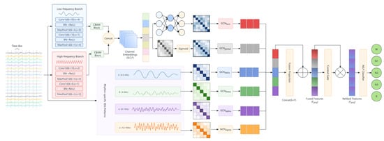
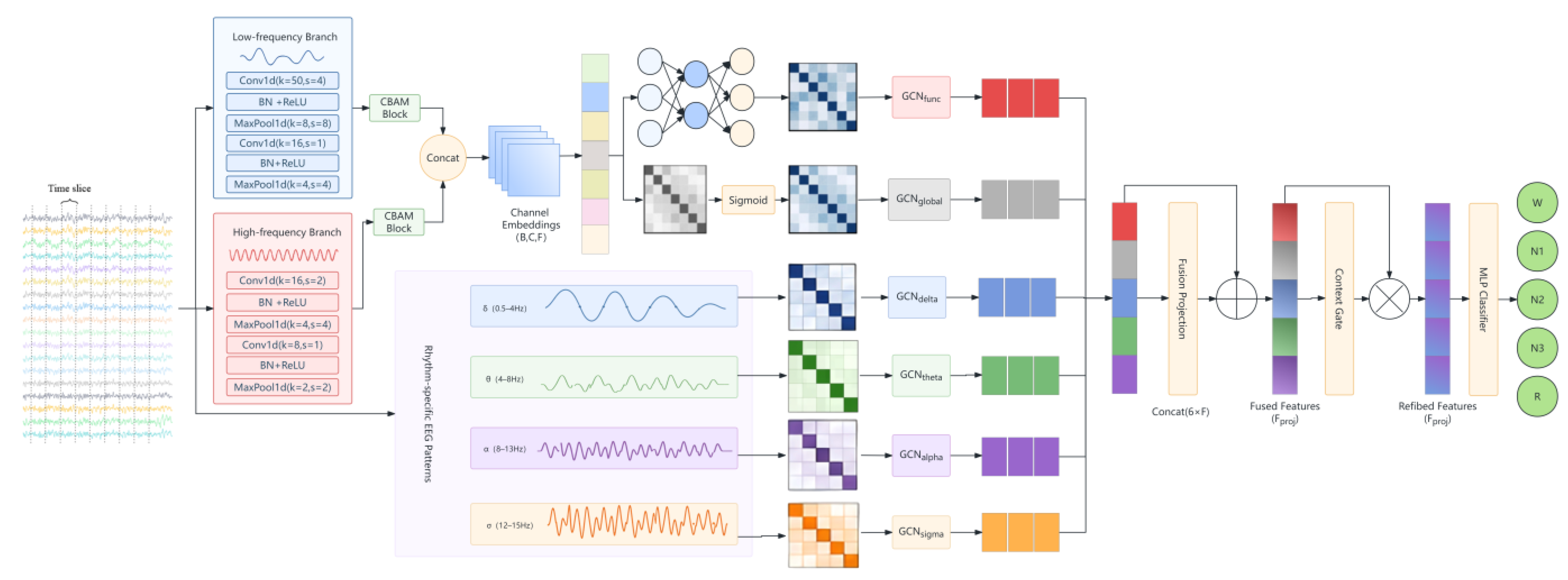
Figure 1 illustrates the overall architecture. Preprocessed EEG sequences are first encoded by a dual-branch 1D-CNN with different temporal receptive fields and CBAM to obtain channel embeddings. Functional adjacency is generated from these embeddings, global adjacency from sample-shared parameters, and four band-specific adjacency matrices from correlations of bandpass-filtered signals. Six independently parameterized GCNs then aggregate the initial channel features along the corresponding views. Finally, graph-level representations are concatenated and recalibrated by elementwise context gating, and an MLP classifier predicts the five sleep stages. The dual-branch encoder provides multiscale temporal features, while frequency-aware graph construction supplies explicit band-specific relationships.

Figure 1. Overall architecture of DCMG-Net. A dual-branch CNN with CBAM extracts broadband channel features. Band-specific adjacency and two data-driven adjacency views define six graph-convolution pathways. Graph-level representations are fused through context gating for classification. DCMG-Net: dual-branch CNN and context-gated multi-view graph network; CBAM: convolutional block attention module.

Each EEG channel is a graph node, and the recordings are segmented into 30 s epochs [1,2]. The five labels are wake (W), NREM stages N1, N2, and N3, and rapid eye movement (REM) sleep. A single sample is represented as

X^(b) ∈ ℝ^C×T,

(1)

where C is the number of EEG channels, T = 30 × f_s is the epoch length, and f_s is the sampling rate. Stacking samples along the batch dimension yields

X ∈ ℝ^B×C×T,

(2)

where B is the batch size. The objective is to learn an end-to-end nonlinear mapping

$ℱ$ : X → Y,

(3)

that maps multichannel EEG signals to a high-dimensional graph representation and predicts the corresponding sleep-stage label:

Y ∈ {W, N1, N2, N3, REM}.

(4)

3.1. Signal Preprocessing and Adaptive Augmentation

To reduce input-scale variation caused by electrode contact and individual amplitude differences [38], Z-score normalization is applied separately to each channel of an input window. For windows containing adjacent epochs, the normalization range follows the context setting. For a single-channel sequence x, normalization is defined as

$${\mathrm{x}}^{\prime }={\displaystyle \frac{\mathrm{x}-{\mathsf{\mu }}_{\mathrm{x}}}{{\mathsf{\sigma }}_{\mathrm{x}}+\mathsf{ϵ}}},$$

(5)

where μ_x and σ_x are the mean and standard deviation of the local EEG segment, respectively, and ϵ is a small constant for numerical stability. This operation produces approximately zero-mean, unit-variance inputs to stabilize training.

During training, probabilistically triggered time warping, Gaussian noise, amplitude scaling, frequency masking, and baseline shifts expand waveform and spectral variability. Each operation acts on a sample copy, with dataset-specific probabilities and magnitudes. Gaussian perturbation is defined as

$${\mathrm{x}}_{\mathrm{aug}}=\mathrm{x}+\mathcal{N}(0,{\mathsf{\sigma }}_{\mathrm{noise}}^2),$$

(6)

where the noise level controls random amplitude perturbations of the input.

Frequency-domain masking reduces reliance on narrow local bands. A fast Fourier transform (FFT) maps the signal to the spectral domain, a randomly selected band of width Δf is masked, and an inverse fast Fourier transform (IFFT) reconstructs the time-domain signal:

x_aug = IFFT(X(f) ⊙ M(f)),

(7)

where ⊙ denotes elementwise multiplication. Random baseline shifts further simulate low-frequency drift associated with electrode-contact changes. A uniformly distributed offset is added to the entire epoch:

δ∼U(−α,α),

(8)

yielding the augmented signal

x_aug = x + δ.

(9)

Time warping changes the local time scale, amplitude scaling changes signal magnitude, frequency masking perturbs local spectral components, and baseline shifts add an epoch-wide offset. Section 5.8 evaluates the complete augmentation pipeline against disabling all augmentation.

3.2. Multiscale Spatiotemporal Feature Extraction

A single temporal scale can be insufficient for representing both long-duration low-frequency dynamics and brief high-frequency events in EEG [7,28]. We therefore use the dual-branch multiscale 1D-CNN shown in Figure 1. For a physical-channel sequence X_i∈ℝ^1×T, two parallel branches extract features. The large-scale branch uses an initial kernel of size 50 and stride 4 to capture long-duration low-frequency patterns, including slow-wave activity in deep sleep [39]. The small-scale branch uses a kernel of size 16 to capture local oscillations such as spindles and transient K-complex morphology [15]. The two branches preserve information at different temporal resolutions.

A one-dimensional CBAM (Convolutional Block Attention Module, CBAM) is applied after each convolutional branch to recalibrate temporal features [20]. For a feature map F ∈ ℝ^D×T′, channel attention first generates M_c∈ℝ^D×1 to emphasize discriminative feature responses. Temporal attention then generates M_t∈ℝ^1×T′ to highlight informative time regions and strengthen the representation of brief EEG events.

The attention-enhanced branch features are concatenated along the feature-channel dimension to obtain F_fused. Global average pooling (GAP) compresses the temporal dimension, followed by a linear projection for dimensional alignment:

H_i = Linear(GAP(F_fused)) ∈ ℝ^F,

(10)

GAP aggregates features over time into a fixed-length representation, which is projected into a common hidden space. Channel features then form the node-feature matrix of one sample:

H^(b) ∈ ℝ^C×F,

(11)

For a batch, H ∈ ℝ^B×C×F. These channel embeddings correspond to the node representations in Figure 1 and serve as the graph-node inputs for subsequent topology modeling.

In the SHHS configuration, channels C4-A1 and C3-A2 each correspond to one graph node. Thus, C = 2, and every view has a 2 × 2 adjacency matrix.

3.3. Frequency-Aware Graph Construction

Given the channel embeddings, the graph-construction module generates six topology views representing input-dependent, sample-shared, and frequency-specific channel relationships:

𝒜 = {A_func, A_global, A_delta, A_theta, A_alpha, A_sigma},

(12)

where A_func and A_global represent data-driven functional connectivity and globally learnable adjacency, respectively; A_delta, A_theta, A_alpha, and A_sigma represent the four physiological frequency-band topologies.

3.3.1. Functional and Globally Learnable Adjacency

The functional view A_func is constructed dynamically from node features. For each node pair (i,j), the concatenated features are passed through a shared MLP to obtain a connection score:

s_ij = MLP([h_i‖h_j]),

(13)

A sigmoid activation produces the adjacency matrix:

$${\mathrm{A}}_{\mathrm{func}}^{(\mathrm{i},\mathrm{j})}=\mathsf{\sigma }({\mathrm{s}}_{\mathrm{ij}}),$$

(14)

where [‖] denotes vector concatenation and σ is the sigmoid function. The resulting functional adjacency varies with sample features and describes channel relationships within the current input. A separate sample-shared global adjacency generates non-negative edge weights from a parameter matrix W_S:

A_global = Sigmoid(W_S),

(15)

The global adjacency is obtained by applying a sigmoid function to a Xavier-initialized parameter matrix shared across samples. It learns channel associations from the training data without an electrode-geometry prior or additional distance, sparsity, or smoothness regularization.

3.3.2. Frequency-Prior Topology Construction

Based on sleep-related rhythms [2,15], four bands are used: delta (0.5–4 Hz), theta (4–8 Hz), alpha (8–13 Hz), and sigma (12–15 Hz). Bandpass filtering uses Hamming-window finite impulse response (FIR) filters with a default kernel duration of 4 s. Kernels are determined by the sampling rate and passband and remain fixed during training. The filtered signal is represented as

X_band ∈ ℝ^C×L,

(16)

where band ∈ {delta,theta,alpha,sigma}. The interchannel covariance matrix is then calculated as

$${\mathsf{\Sigma }}_{\mathrm{band}}={\displaystyle \frac{1}{\mathrm{L}-1}}({\mathrm{X}}_{\mathrm{band}}-{\mathsf{\mu }}_{\mathrm{band}})({\mathrm{X}}_{\mathrm{band}}-{\mathsf{\mu }}_{\mathrm{band}}{)}^{\mathrm{T}}$$

(17)

Pearson correlations are computed from channel covariance and variance to obtain a correlation matrix for each band:

$${\mathrm{R}}_{\mathrm{band}}={\mathrm{D}}_{\mathrm{band}}^{-\frac{1}{2}}{\mathsf{\Sigma }}_{\mathrm{band}}{\mathrm{D}}_{\mathrm{band}}^{-\frac{1}{2}},$$

(18)

where D_band is the diagonal variance matrix.

To obtain nonnegative propagation weights, Pearson correlations are linearly mapped to [0,1]. Zero correlation maps to 0.5, negative correlations to weights below 0.5, and positive correlations to weights above 0.5, encoding correlation strength in the graph-propagation weights:

$${\mathrm{A}}_{\mathrm{band}}={\displaystyle \frac{1}{2}}({\mathrm{R}}_{\mathrm{band}}+1),$$

(19)

This yields the four band-specific topologies A_delta, A_theta, A_alpha, and A_sigma. Each adjacency matrix modulates graph propagation, while all node inputs use shared broadband channel embeddings. Band-specific relationships and temporal features are thereby modeled jointly during graph encoding.

3.4. Multi-View Graph Convolutional Encoding

As shown in Figure 1, each topology view is processed by an independent GCN to learn topology-specific spatial representations. Given H ∈ ℝ^B×C×F and the six views, six parallel, independently parameterized encoders model channel interactions under the respective connectivity patterns.

For each view v ∈ {func, global, delta, theta, alpha, sigma}, self-loops are first added to the adjacency matrix:

$${\tilde{\mathrm{A}}}_{\mathrm{v}}={\mathrm{A}}_{\mathrm{v}}+\mathrm{I},$$

(20)

where I is the identity matrix. The degree matrix is constructed as

$${\tilde{\mathrm{D}}}_{\mathrm{v}}(\mathrm{i},\mathrm{i})={\sum }_{\mathrm{j}}{\tilde{\mathrm{A}}}_{\mathrm{v}}(\mathrm{i},\mathrm{j}),$$

(21)

followed by symmetric degree normalization:

$${\widehat{\mathrm{A}}}_{\mathrm{v}}={\tilde{\mathrm{D}}}_{\mathrm{v}}^{-1/2}{\tilde{\mathrm{A}}}_{\mathrm{v}}{\tilde{\mathrm{D}}}_{\mathrm{v}}^{-1/2},$$

(22)

The normalized adjacency is the propagation matrix. Node features are first linearly projected, and subsequent aggregation uses a rectified linear unit (ReLU). The linear projection is

Z^(v) = HW_v,

(23)

where W_v∈ℝ^F×F′ is a learnable projection matrix. Neighborhood aggregation is then performed as

$${\mathrm{H}}^{\left(\mathrm{v}\right)}=\mathrm{ReLU}\left({\widehat{\mathrm{A}}}_{\mathrm{v}}{\mathrm{Z}}^{\left(\mathrm{v}\right)}\right),$$

(24)

where Z^(v)∈ℝ^B×C×F′ is the intermediate feature tensor.

To preserve pre-aggregation information and alleviate representation homogenization in stacked graph convolutions [40], a residual connection is added after spatial aggregation:

$${\mathrm{\Phi }}_{\mathrm{res}}(\mathrm{H})=\left\{\begin{array}{c}\mathrm{H},\mathrm{F}={\mathrm{F}}^{\prime }\\ \mathrm{H}{\mathrm{W}}_{\mathrm{res}},\mathrm{F}\ne {\mathrm{F}}^{\prime }\end{array}\right.,$$

(25)

where W_res∈ℝ^F×F′ is an independent residual projection. Node representations are updated as

H^(v) ← ReLU(H^(v) + Φ_res(H)).

(26)

Layer normalization (LayerNorm) and dropout are then applied to improve training stability and generalization.

After node-level updates, graph-level representations are obtained by global average pooling:

$${\mathrm{emb}}_{\mathrm{v}}={\displaystyle \frac{1}{\mathrm{C}}}{\sum }_{\mathrm{i}=1}^{\mathrm{C}}{\mathrm{H}}_{:,\mathrm{i},:}^{\left(\mathrm{v}\right)},$$

(27)

where emb_v∈ℝ^B×F′ is the graph-level representation of view v used for subsequent fusion.

3.5. Adaptive Fusion with Context Gating

Miech et al. introduced context gating for video classification, using input activations to generate elementwise self-recalibration coefficients [19]. Because the operation acts on feature vectors rather than video-specific spatial structures, it can be transferred to joint EEG representations. In this case, six graph views provide complementary features. Their joint representation captures conditional dependencies across dimensions, and sigmoid coefficients adapt their magnitudes to the input. A bottleneck projection controls the gate’s parameter count.

The six graph embeddings are first concatenated along the feature dimension to form a joint representation of topology and frequency information:

H_concat = Concat(emb_func, emb_global, emb_delta, emb_theta, emb_alpha, emb_sigma)

(28)

where H_concat∈ℝ^B×6F′, B is the batch size, and F′ is the feature dimension of one graph view. The concatenated representation is projected into a P-dimensional fusion space:

F_proj = Linear(H_concat),

(29)

Let F_proj∈ℝ^B×P. With a bottleneck compression ratio r, the intermediate dimension is

$$\mathrm{d}=\frac{\mathrm{P}}{\mathrm{r}}$$

(30)

where r is the compression ratio. Gating weights are calculated as

Z_gate = ReLU(LayerNorm(F_projW_down)),

(31)

G = Sigmoid(Z_gateW_up),

(32)

where W_down∈ℝ^P×d, W_up∈ℝ^d×P, and d = $\frac{\mathrm{P}}{\mathrm{r}}$. The gate projects the fused features into a compressed space and restores them to P dimensions, producing elementwise coefficients G ∈ ℝ^B×P in [0,1] to adaptively modulate the representation.

The dynamic weights are applied through the elementwise Hadamard product:

F_refined = F_proj ⊙ G,

(33)

In this module, context refers to the joint feature representation. For a single-epoch input, weights are generated from the current epoch’s multichannel, multi-view information. With multiple epochs, the joint representation also includes adjacent-epoch information, allowing recalibration to adapt to the input configuration.

Temporal context length L is a dataset-specific input hyperparameter, defined as the number of consecutive 30 s epochs supplied to the shared encoder. Candidate lengths are 1, 3, 5, and 7 for Sleep-EDF-20 and 1, 3, and 5 for ISRUC-S3 and SHHS. Each dataset’s length is selected by Macro-F1 on the internal validation set within the outer training partition and fixed before evaluation on the held-out test set. The selected lengths are 1 epoch (30 s) for ISRUC-S3, 5 epochs (150 s) for Sleep-EDF-20, and 3 epochs (90 s) for SHHS. Test data are used only for final reporting and do not guide context-length adjustment.

Channel configuration motivates evaluating these lengths independently. ISRUC-S3 provides six EEG channels and therefore richer interchannel information within one epoch; its validation results favor a single epoch over longer windows. Sleep-EDF-20 and SHHS use two channels, making adjacent-epoch information a useful complement to their more limited channel coverage. Their validation results favor five and three epochs, respectively. The context-length sensitivity analysis is presented in Section 5.8. Longer context may provide additional temporal information but can also introduce irrelevant variability from neighboring epochs. Channel count motivates the comparison; internal-validation performance determines the final choice.

3.6. Classification and Class-Imbalance-Aware Optimization

The gated features are passed to an MLP classification head comprising linear projection, LayerNorm, ReLU, and dropout, followed by a five-class output layer. The label set is

Y ∈ {W, N1, N2, N3, REM},

(34)

The head outputs five logits, which are converted to class probabilities by SoftMax.

Sleep datasets typically exhibit substantial class imbalance [41,42], with transitional stages such as N1 less frequent than W and N2 [3,43]. Models may consequently favor majority classes and underperform on minority stages. We address this through both sampling and loss optimization.

During data loading, class-balanced weighted sampling is based on the effective number of samples. For class c with N_c training samples, the class weight is defined as

$${\mathrm{class}\text{\_}\mathrm{weight}}_{\mathrm{c}}=\frac{1-\mathsf{\beta }}{1-{\mathsf{\beta }}^{{\mathrm{N}}_{\mathrm{c}}}},$$

(35)

where β ∈ [0,1) is a smoothing hyperparameter; β = 0.995 in the ISRUC-S3 configuration. A power p further controls weighting strength, yielding the sampling weight

w^sample = (class_weight_y)^p,

(36)

The sampling power p regulates how strongly class weights influence sample selection. At p = 0, all training samples are sampled equally; larger p increases the influence of class weighting. The powers are 0, 0.65, and 0.4 for Sleep-EDF-20, ISRUC-S3, and SHHS, respectively.

Configurations using focal loss employ weighted focal loss [44] to emphasize difficult examples and minority classes. Let $p_{y_i}$ be the probability assigned to the true class y_i of sample i, and ${w_{y_i}}^{\mathit{loss}}$ its class weight. The loss is

$${\mathcal{L}}_{\mathrm{Focal}}=-{\displaystyle \frac{1}{\mathrm{N}}}{\sum }_{\mathrm{i}=1}^{\mathrm{N}}{\mathrm{w}}_{{\mathrm{y}}_{\mathrm{i}}}^{\mathrm{loss}}(1-{\mathrm{p}}_{{\mathrm{y}}_{\mathrm{i}}}{)}^{\mathsf{\gamma }}\log (\mathrm{p}{\mathrm{y}}_{\mathrm{i}}),$$

(37)

where N is the batch size and γ is the focusing parameter. The ISRUC-S3 default is γ = 1.2, selected based on internal-validation performance. The focal term reduces the relative contribution of easy examples, while class weights adjust the contribution of each class.

Training uses Adam with decoupled weight decay (AdamW) [45], exponential moving average (EMA) weights, learning-rate scheduling, and early stopping. Sampling powers and the ISRUC-S3 focal-loss setting are presented above; The internal-validation results for hyperparameter selection are presented in Section 5.7.

4. Experimental Setup

4.1. Datasets

We evaluated EEG-only staging on Sleep-EDF-20, ISRUC-S3, and SHHS. Recordings are divided into 30 s epochs labeled W, N1, N2, N3, and REM. Subject-independent outer cross-validation is used, with a separate validation set in each fold. All recordings from one subject remain in the same partition, and all models use identical partition lists. Training data update model parameters; validation macro-averaged F1 (Macro-F1 or MF1) selects checkpoints and controls early stopping; test data evaluate only the selected checkpoint. Dataset sizes and stage distributions are summarized in Table 1.

Table 1. Dataset characteristics and sleep-stage distributions.

Dataset	Epochs	Subjects	W	N1	N2	N3	REM
Sleep-EDF-20	42,308	20	8285 19.6%	2804 6.6%	17,799 42.1%	5703 13.5%	7717 18.2%
ISRUC-S3	17,778	10	3519 19.8%	2371 13.3%	5528 31.1%	4011 22.6%	2349 13.2%
SHHS	324,854	329	46,319 14.3%	10,304 3.2%	142,125 43.8%	60,153 18.5%	65,953 20.3%

Sleep-EDF-20 includes 20 subjects and two EEG channels, Fpz-Cz and Pz-Oz, sampled at 100 Hz [43,46]. Preprocessing retains 42,308 epochs. Subject-independent outer 20-fold testing holds out one subject per fold. A separate validation subset is selected from the remaining 19 subjects, with the rest used for training. Multiple nights from the same subject remain together. Across 20 folds, each subject appears in the outer test set exactly once.

ISRUC-S3 includes 10 healthy subjects and six EEG channels: F3-A2, C3-A2, O1-A2, F4-A1, C4-A1, and O2-A1, sampled at 200 Hz [41]. Preprocessing retains 17,778 epochs. Subject-independent outer 10-fold testing holds out one subject per fold, with a separate validation subset drawn from the remaining nine subjects and the rest used for training. Each subject appears in the outer test set exactly once.

For SHHS, 329 subjects are selected, with one recording per subject. The C4–A1 and C3–A2 EEG channels, labeled “EEG” and “EEG(sec)” in the source recordings, respectively, were sampled at 125 Hz [42], yielding 324,854 epochs after preprocessing. Subject-independent outer 20-fold testing uses nine test groups of 17 subjects and eleven of 16. Each fold holds out one group for testing and selects 30 validation subjects from the remaining subjects using predefined lists. Thus, nine folds contain 282 training, 30 validation, and 17 test subjects; the other eleven contain 283, 30, and 16, respectively, totaling 329 subjects per fold. The three partitions are mutually exclusive and shared across models. Every subject appears in the outer test set once.

Preprocessing trims wake periods at the recording boundaries [47] and normalizes signals channelwise. Stages S3 and S4 in Rechtschaffen and Kales (R&K) annotations are merged into N3. Adjacent epochs follow their stored order within each file to form context windows. Filtering and resampling comparisons are applied to the prepared epochs.

4.2. Implementation Details

The experiments used an Ubuntu server with an NVIDIA RTX 3090, Python 3.10.22, PyTorch 2.5.1, and CUDA 12.4. The global random seed was 123. Reported results correspond to this seed and do not include means and standard deviations across repeated training runs with different seeds.

Training, validation, and testing are strictly separated. Data are loaded by subject ID, and only training samples update parameters. Validation Macro-F1 is computed after each epoch, retaining the checkpoint with the highest score; ties retain the earlier checkpoint. The selected weights are then evaluated on the test set using overall accuracy (ACC), Macro-F1, κ, and N1-F1. Validation samples do not contribute gradients but guide model selection. Reported test results are not subsequently used to tune hyperparameters or replace checkpoints.

Within each dataset, models use consistent training settings and class-weighted classification losses, with at most 100 epochs. AdamW uses AMSGrad and a weight decay of 1 × 10⁻⁴. Section 5.7 reports ISRUC-S3 sensitivity to feature dimension, gate compression ratio, dropout, the focal-loss parameter, and sampling power.

Model selection uses the EMA checkpoint with the highest internal-validation Macro-F1, retaining the earlier epoch in a tie. Before validation, batch normalization (BN) statistics are re-estimated using unaugmented training samples only, without changing trainable weights. Models within each dataset share the same selection and output-processing procedures for structural comparisons.

4.3. Evaluation Metrics

Performance is assessed using standard sleep-staging metrics [22,35]: ACC (Overall Accuracy, ACC), MF1 (Macro F1-score, MF1), Cohen’s κ (Cohen’s Kappa), and per-class F1 scores.

For five-class staging, let C = 5 denote the number of stages. For class i∈{W,N1,N2,N3,REM}, TP_i, FP_i, TN_i, and FN_i denote the numbers of true positives, false positives, true negatives, and false negatives, respectively [48]. The metrics are defined below.

4.3.1. Overall Accuracy

ACC is the proportion of correctly classified epochs and measures global prediction accuracy:

$$\mathrm{ACC}={\displaystyle \frac{{\sum }_{\mathrm{C}=1}^{\mathrm{K}}\mathrm{T}{\mathrm{P}}_{\mathrm{C}}}{\mathrm{N}}},$$

(38)

where K is the number of sleep stages, N is the total number of test epochs, and TP_c is the number of correctly classified epochs in stage c.

4.3.2. Macro-F1 Score

Accuracy alone does not fully characterize performance on class-imbalanced PSG data. MF1 therefore complements accuracy [16,41]. Precision P_i and recall R_i are calculated for each class, and MF1 is the arithmetic mean of the classwise F1 scores:

$${\mathrm{Precision}}_{\mathrm{i}}=\frac{\mathrm{T}{\mathrm{P}}_{\mathrm{i}}}{\mathrm{T}{\mathrm{P}}_{\mathrm{i}}+\mathrm{F}{\mathrm{P}}_{\mathrm{i}}},{\mathrm{Recall}}_{\mathrm{i}}=\frac{\mathrm{T}{\mathrm{P}}_{\mathrm{i}}}{\mathrm{T}{\mathrm{P}}_{\mathrm{i}}+\mathrm{F}{\mathrm{N}}_{\mathrm{i}}},$$

(39)

$$\mathrm{F}{1}_{\mathrm{i}}=2\times \frac{{\mathrm{Precision}}_{\mathrm{i}}\times {\mathrm{Recall}}_{\mathrm{i}}}{{\mathrm{Precision}}_{\mathrm{i}}+{\mathrm{Recall}}_{\mathrm{i}}},\mathrm{MF}1=\frac{1}{\mathrm{C}}{\sum }_{\mathrm{i}=1}^{\mathrm{C}}\mathrm{F} 1_{\mathrm{i}},$$

(40)

Per-class F1 scores are also reported to characterize discrimination between individual sleep stages.

4.3.3. Cohen’s Kappa

Cohen’s κ measures agreement between predictions and reference annotations after correcting for chance agreement based on their marginal distributions [48,49]. Because κ is also influenced by class distribution, it is interpreted alongside ACC, MF1, and per-class F1:

$$\mathsf{\kappa }=\frac{{\mathrm{p}}_{\mathrm{o}}-{\mathrm{p}}_{\mathrm{e}}}{1-{\mathrm{p}}_{\mathrm{e}}},$$

(41)

where p_o is observed agreement, equivalent to ACC, and p_e is expected agreement under the marginal distributions of predictions and annotations. Values closer to 1 indicate greater agreement with the reference scoring.

5. Results and Discussion

5.1. Overall Classification Performance

Table 2 summarizes DCMG-Net and representative methods on the three datasets using ACC, MF1, Cohen’s κ, and per-stage F1. Comparator results are taken from the respective publications, whereas DCMG-Net results are from the present experiments. Overall and stage-specific performance are considered below.

Table 2. Overall and per-stage classification performance on three datasets. ACC, MF1, and per-class F1 are percentages; κ is reported as a decimal.

Dataset	Method	Overall Metrics			Per-Class F1-Score
		Acc	MF1	k	W	N1	N2	N3	REM
Sleep-edf-20	DeepSleepNet [6]	81.9	76.6	0.76	86.7	45.5	85.1	83.3	82.6
	SleepEEGNet [50]	81.5	76.6	0.75	89.4	44.4	84.7	84.6	79.6
	RestnetLSTM [51]	82.5	73.7	0.76	86.5	28.4	87.7	89.8	76.2
	MultitaskCNN [52]	83.1	75.0	0.77	87.9	33.5	87.5	85.8	79.0
	AttnSleep [10]	84.4	78.1	0.79	89.7	42.6	88.8	90.2	79.0
	SeqSleepNet [28]	84.6	78.0	0.79	87.7	43.8	88.2	86.5	84.0
	CTCNet [23]	86.2	82.5	0.82	92.2	57.6	89.8	89.6	82.8
	WASR-LCNN [53]	87.6	82.1	0.83	87.6	51.6	88.0	88.1	85.0
	DCMG-Net (ours)	91.2	84.4	0.88	98.7	52.9	91.9	93.6	84.8
ISRUC-S3	DeepSleepNet [6]	78.8	77.9	0.73	88.7	60.2	74.6	85.8	80.2
	SeqSleepNet [28]	78.9	76.3	0.72	83.6	43.9	79.3	87.9	86.7
	GraphSleepNet [11]	79.9	78.7	0.74	87.8	57.4	77.6	86.4	84.1
	MSTGCN [29]	82.1	80.8	0.76	89.4	59.6	80.6	89.0	85.6
	MVF-SleepNet [13]	84.1	82.8	0.79	90.0	62.5	83.3	91.1	87.3
	StAGN [37]	84.4	83.6	-	90.7	66.3	83.2	89.5	88.1
	DGraphormer-SleepNet [54]	85.4	84.5	-	91.9	67.6	83.8	90.7	88.3
	cVAN [55]	85.6	84.2	0.81	91.5	67.4	84.4	91.1	86.4
	DCMG-Net (ours)	90.0	88.7	0.87	93.3	70.1	90.2	93.9	95.9
SHHS	SleepEEGNet [50]	73.9	68.4	0.65	81.3	34.4	73.4	75.9	77.0
	DeepSleepNet [6]	81.0	73.9	0.73	85.4	40.5	82.5	79.3	81.9
	AttnSleep [10]	84.2	75.3	0.78	86.7	33.2	87.1	87.1	82.1
	SleepFCN [8]	81.3	72.0	0.74	81.7	29.0	85.4	84.1	79.6
	MFCC-CNN-LSTM [56]	82.4	75.0	-	93.8	27.1	79.5	64.1	82.2
	PFTSleep [25]	86.0	76.5	0.80	92.1	35.9	86.4	78.2	89.8
	DCMG-Net (ours)	86.3	77.2	0.87	87.5	33.6	87.8	85.4	91.7

Note: Bold values indicate the best performance, and underlined values indicate the second-best performance for each metric within each dataset. Tied values share the same formatting.

On Sleep-EDF-20, DCMG-Net achieves an ACC of 91.2%, an MF1 of 84.4%, and κ = 0.88. F1 scores for W, N1, N2, N3, and REM are 98.7%, 52.9%, 91.9%, 93.6%, and 84.8%, respectively. The high F1 scores for W, N2, and N3 indicate effective discrimination of wakefulness and stable NREM stages.

On ISRUC-S3, ACC, MF1, and κ reach 90.0%, 88.7%, and 0.87, with stagewise F1 scores of 93.3%, 70.1%, 90.2%, 93.9%, and 95.9%, indicating relatively balanced discrimination across stages. On SHHS, the corresponding overall metrics are 86.3%, 77.2%, and 0.81; stagewise F1 scores are 87.5%, 33.6%, 87.8%, 85.4%, and 91.7%. In particular, the REM F1 of 91.7% demonstrates effective representation with two EEG channels.

These results show that DCMG-Net can combine band-specific topology and channel features for five-class staging. The following analyses examine model size, stage sequences, confusion patterns, and structural comparisons to further characterize its predictions.

5.2. Model Complexity

Table 3 compares parameter counts and computational costs. Parameters are reported in millions (M) and computation in millions of floating-point operations (MFLOPs). Complexity values for SalientSleepNet, SleepPrintNet, and DynamicSleepNet were taken from the common analysis in [57]; the original SleepPrintNet architecture is described in [58]. DCMG-Net is measured using each dataset’s default configuration, counting convolutions, linear layers, and matrix multiplications. One multiply–accumulate operation (MAC) is counted as two floating-point operations (FLOPs).

Table 3. Parameter counts (M) and computational costs (MFLOPs) of different methods.

Method	Single-Channel Reference	ISRUC-S3	Sleep-EDF-20	SHHS
AttnSleep [10]	0.522805/122.5	—	—	—
HierCorrPool [59]	8.15/82.9	13.29/499.0	8.93/146.1	—
FC-STGNN [60]	0.45799/46.2	3.2/475.8	1.37/186.6	—
cVAN [55]	—	6.834571/483.4	5.699173/273.4	—
SalientSleepNet [57]	—	1.18/886.406 *	1.18/443.438 *	—
SleepPrintNet [58]	—	9.97/188.711 *	5.64/84.141 *	—
DynamicSleepNet [57]	—	1.40/48.438 *	1.29/40.156 *	—
DCMG-Net (ours)	0.267331/23.039	0.730694/278.726	0.267334/227.136	0.267334/170.787

Note: Cells report parameters (M)/computation (MFLOPs); ‘—’ indicates an unreported value. DCMG-Net uses dataset-default settings and per-sample computation with 1 MAC = 2 FLOPs. The single-channel column is a complexity reference. * Approximate per-sample computational costs, calculated by dividing the totals reported for 256 samples in [57] by 256. The source’s ISRUC configuration uses subgroup 1.

DCMG-Net uses 0.730694, 0.267334, and 0.267334 M parameters for ISRUC-S3, Sleep-EDF-20, and SHHS, with computational costs of 278.726, 227.136, and 170.787 MFLOPs, respectively. Counts cover modules used in the complete model’s forward pass and exclude the separate head used only for the CNN ablation. Fixed filter coefficients are not trainable parameters. The per-view feature dimension is 128 for ISRUC-S3 and 64 for the other datasets. Increasing this dimension expands the functional-graph MLP, six GCNs, gating layers after concatenation, and classifier. Thus, the higher ISRUC-S3 parameter count primarily reflects the hidden feature dimension rather than context length or a direct dependence of GCN weights on node count.

The configurations differ by 463,360 parameters: 74,880 in the six GCNs, 221,856 in gating, 137,600 in the classifier, and 28,992 in the front-end projection and functional-graph MLP. Expanding global adjacency from 2 × 2 to 6 × 6 adds only 32 parameters. GCN projection dimensions depend on input and output feature dimensions. Context lengths are 1, 5, and 3 epochs for ISRUC-S3, Sleep-EDF-20, and SHHS, respectively. Adjacent epochs are processed and aggregated with a shared encoder; so, context length changes computation and input coverage without directly adding these trainable parameters.

For the additional literature configurations, the reported computation for 256 samples is divided by 256 to obtain per-sample MFLOPs. Raw parameter counts are converted to M, while values originally reported in M retain their precision. The table includes a single-channel reference and dataset-specific configurations to show parameter–computation trade-offs.

5.3. Sleep-Stage Sequence Visualization

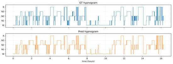
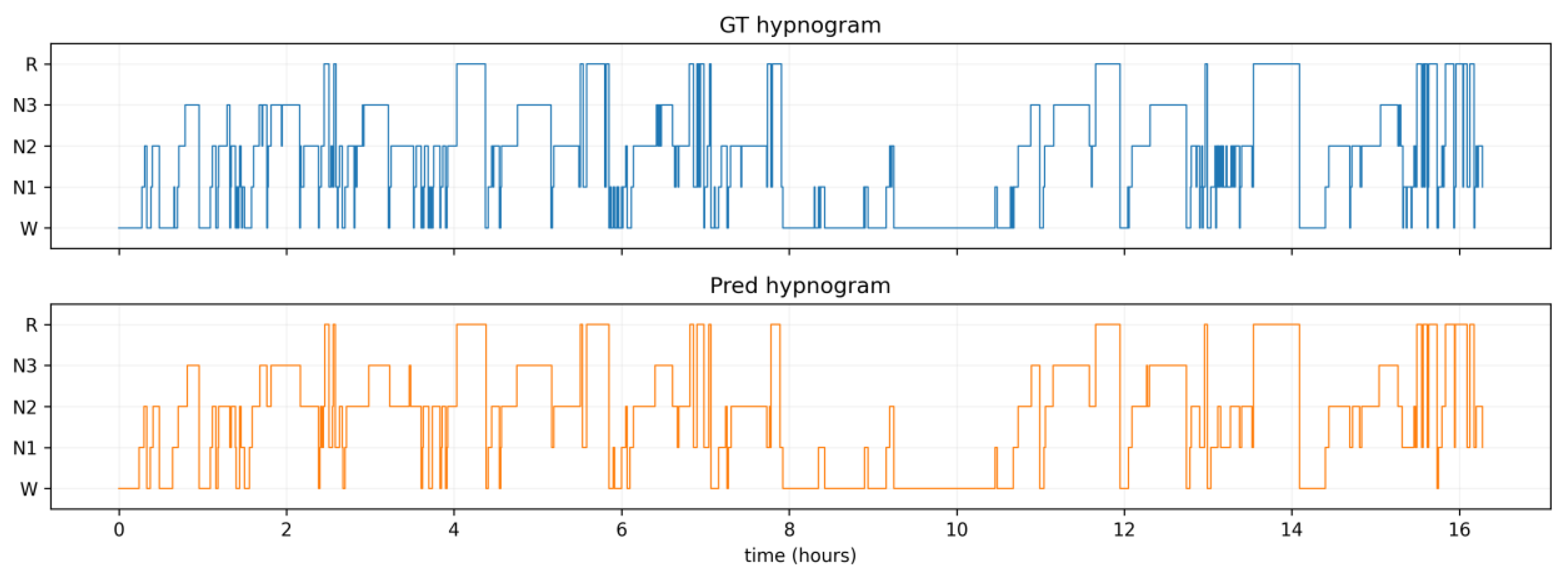
Figure 2 compares reference sleep-stage labels with DCMG-Net predictions. The upper panel shows the reference sequence and the lower panel the predictions; the vertical axis lists W, N1, N2, N3, and REM. Agreement across several sustained intervals illustrates the model’s representation of stage distributions and transition locations.

Figure 2. Example sleep-stage sequences from manual annotations (top) and DCMG-Net predictions (bottom).

The sustained intervals and transitions show that the model follows changes in sleep stage while maintaining continuity across major stage intervals. This temporal visualization complements the overall classification results.

5.4. Confusion Matrix Analysis

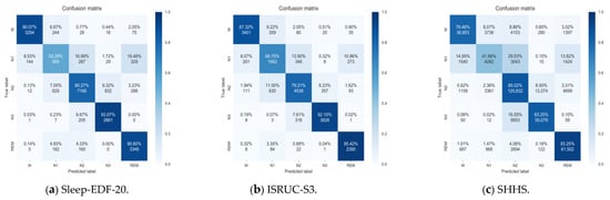
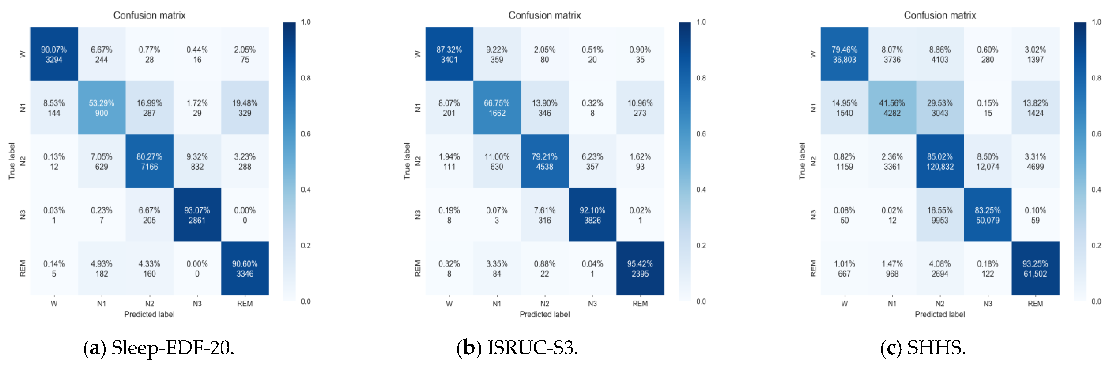
Figure 3 presents the stage-confusion patterns across the three datasets. Overall, predictions are concentrated along the diagonal, although the degree of dispersion differs between stages. On Sleep-EDF-20, the predictions for W, N3, and REM are relatively concentrated, whereas N1 is more easily confused with other stages, being misclassified mainly as REM and N2, with some instances also misclassified as W. This indicates that the discriminative boundaries between N1 and these classes remain insufficiently clear.

Figure 3. Row-normalized confusion matrices: (a) Sleep-EDF-20, (b) ISRUC-S3, and (c) SHHS. Rows indicate true stages and columns indicate predicted stages; diagonal entries denote recall.

On ISRUC-S3, REM predictions are concentrated in the correct class, and N1 predictions are also more concentrated than on Sleep-EDF-20. Bidirectional cross-classification persists between N2 and N3, suggesting that the model’s ability to distinguish these two stages can still be improved. This observation is consistent with the gradual variation of EEG features across different levels of sleep depth.

On SHHS, the predictions for REM, N2, and N3 are relatively concentrated, while those for N1 are more dispersed, being misclassified mainly as N2, W, and REM. In addition, the confusion between N2 and N3 is more pronounced in the form of N3 being predicted as N2. Thus, although the model captures discriminative features for the major sleep stages, its ability to separate N1 and neighboring stage boundaries remains limited under this dual-channel configuration.

Taken together, the confusion matrices show that the model’s recognition ability varies across stages: REM and several NREM stages exhibit concentrated prediction distributions, while N1 is the most prominent source of error. The confusion patterns also differ between datasets; so, the performance differences cannot be explained by the number of channels alone. Future work could focus on separating N1 from its confusable classes, refining feature representations by incorporating sleep-event annotations and contextual modelling.

5.5. Multi-View Response Analysis

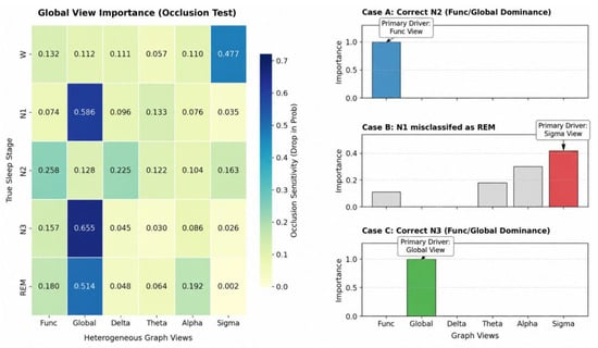
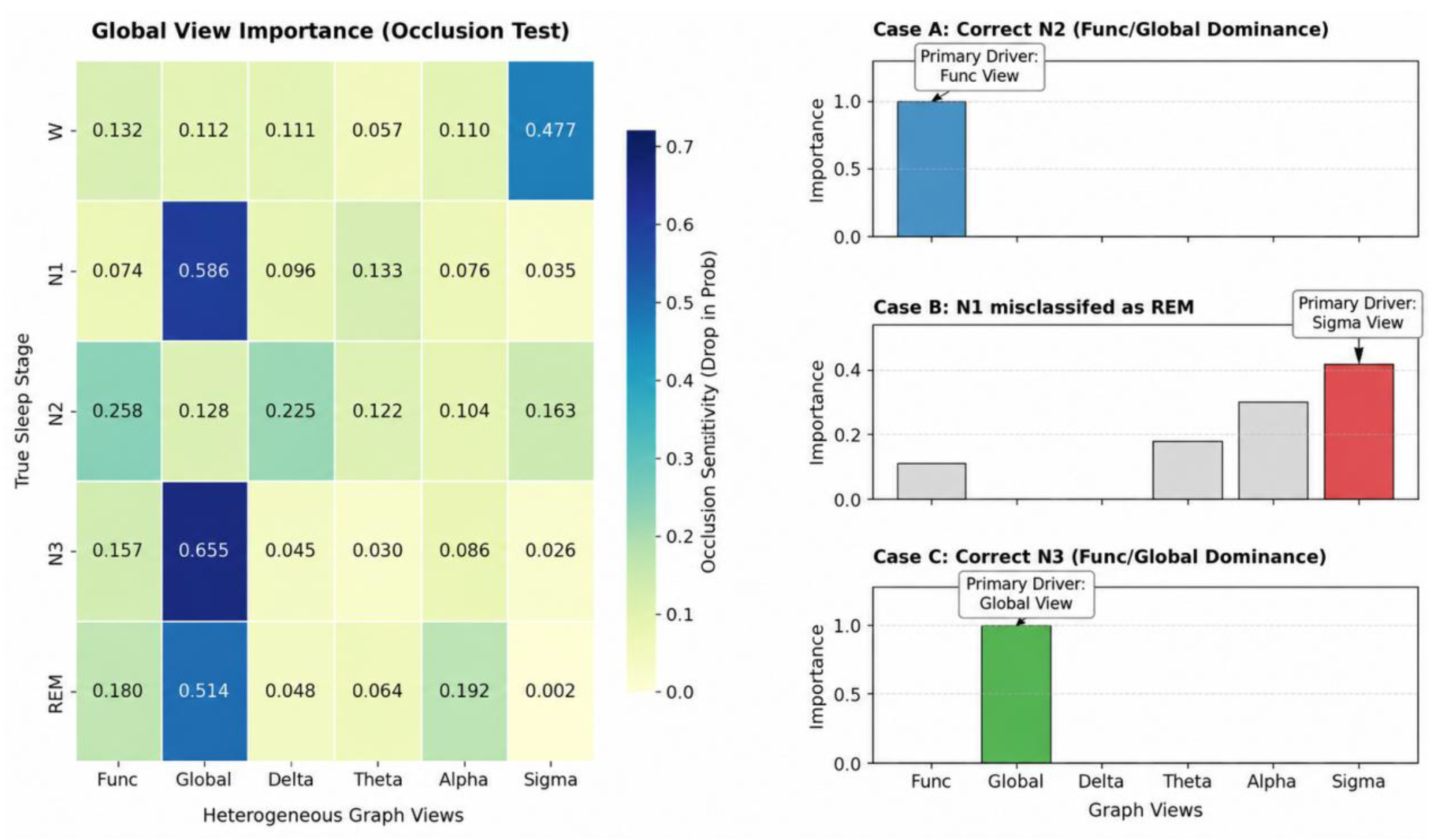
Figure 4 combines view-occlusion sensitivity with sample-level gating responses to show how different feature sources are used. Occlusion removes a view representation and examines output changes, while gating responses show adaptive recalibration of joint features. Global denotes sample-shared learnable adjacency generated by applying a sigmoid to a parameter matrix.

Figure 4. Multi-view occlusion sensitivity and example gating weights. Global denotes the sample-shared learnable adjacency.

View responses differ across stages. Global-view occlusion sensitivity is 0.655 for N3, indicating that predictions respond strongly to this representation. Sample-level gating distributions show that feature weights change with the input. Together, these analyses illustrate differentiated use of multi-view information during fusion.

5.6. Adjacency Matrix Visualization

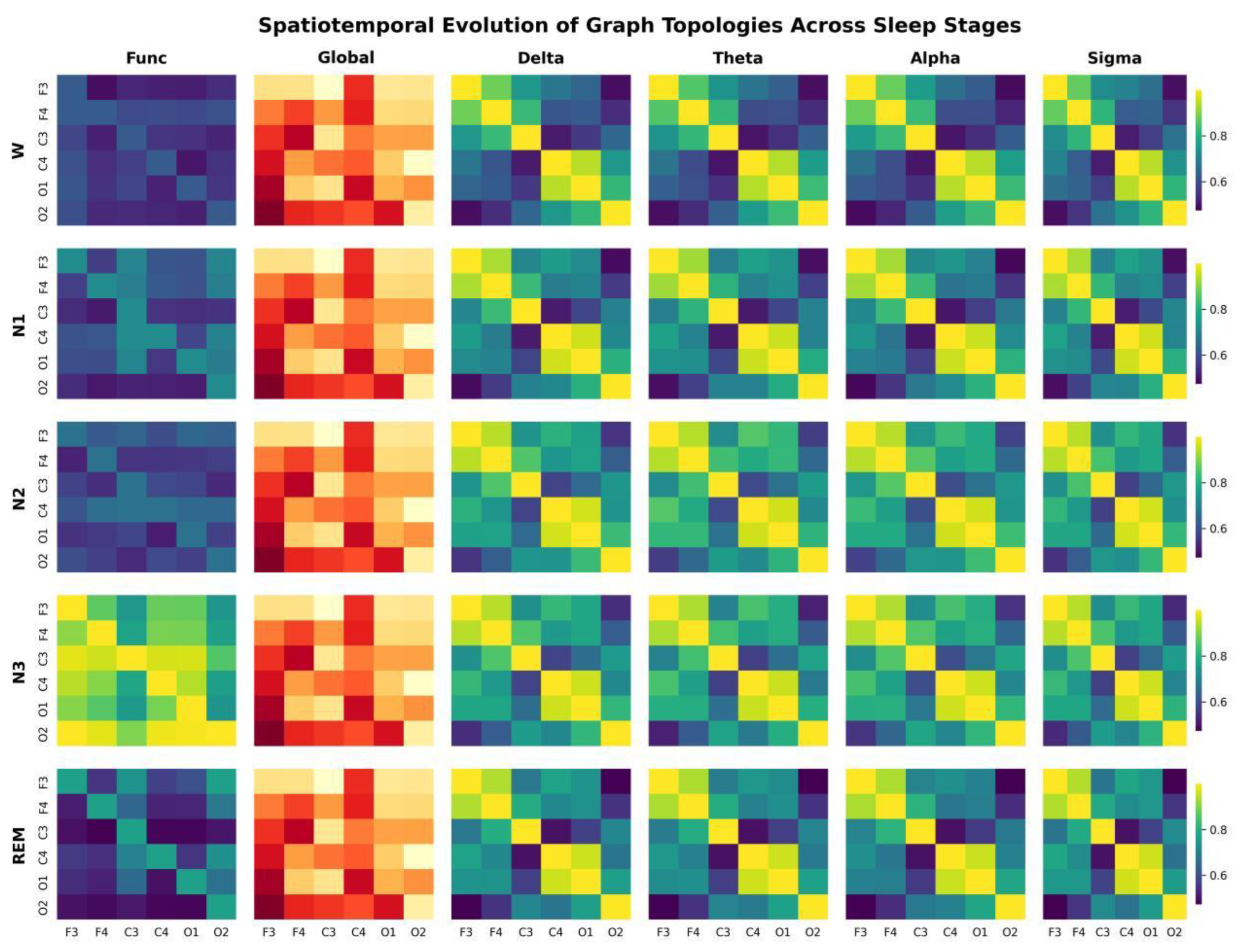
Figure 5 shows mean adjacency matrices for each view across the five stages, with colors indicating channel-edge weights. Functional adjacency is generated from input features; band-specific views represent correlations between filtered channels; and global learnable adjacency provides sample-shared associations.

Figure 5. Stage-wise mean multi-view adjacency matrices. Global denotes the sample-shared learnable adjacency; colors indicate channel edge weights. The Global view uses a yellow–orange–red color scale, whereas the other views use a purple–blue–green–yellow color scale. The color scales should be interpreted separately for each view.

Functional and band-specific adjacency vary with the input and exhibit stage-dependent weight distributions. Global adjacency shares parameters across samples and supplies consistent channel relationships across stages. Input-dependent and shared relationships therefore provide complementary topological information for fusion.

5.7. Ablation Study

The experiments address three questions: how individual components change performance, how multi-view information should be fused, and whether graph aggregation offers advantages over alternative architectures. Incremental ablations on ISRUC-S3 first examine attention, functional graphs, multiple views, and gating. The same progression is then evaluated on two-channel SHHS, with feature visualization used to examine representation changes. Finally, alternative-architecture comparisons and internal-validation hyperparameter analyses assess graph encoding and configuration choices.

Five incremental variants are evaluated. CNN is the basic multiscale encoder. CNN + CBAM tests attention-based recalibration. Functional GCN adds functional-graph aggregation to examine channel-relationship modeling. Multi-view GCN + concatenation adds globally learnable and four band-specific adjacency matrices to examine joint representation of multiple topologies. The complete DCMG-Net adds context gating to compare adaptive fusion with direct concatenation.

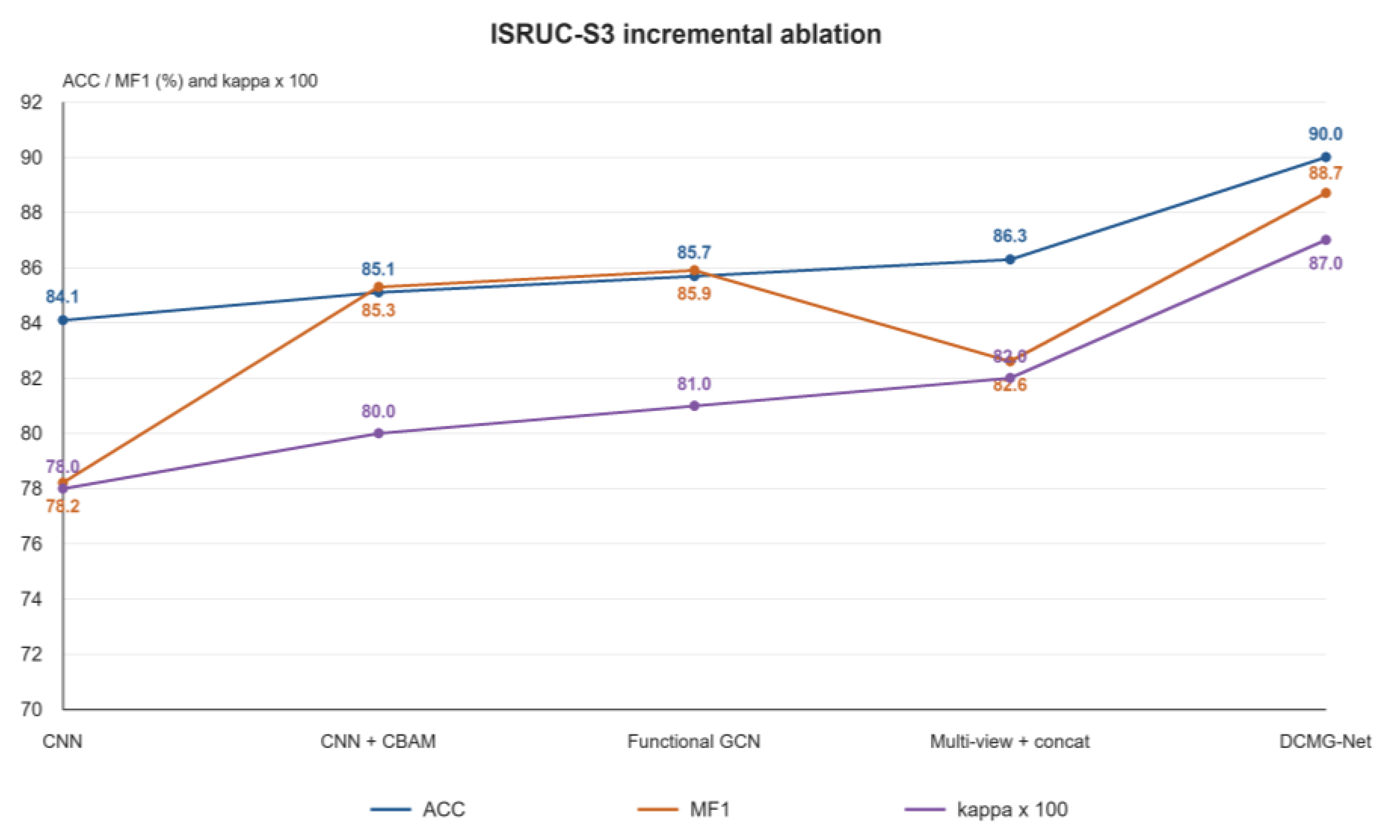
Figure 6 presents the ISRUC-S3 ablation. The baseline CNN achieves ACC = 84.1% and MF1 = 78.2%. Adding CBAM increases these to 85.1% and 85.3%, improving MF1 by 7.1 percentage points and indicating better feature representation in this comparison. Functional GCN further increases ACC and MF1 to 85.7% and 85.9%; the additional 0.6-point MF1 gain shows the supplementary contribution of channel aggregation.

Figure 6. Incremental ablation results on ISRUC-S3. ACC and MF1 are percentages; kappa is multiplied by 100 for display.

Direct multi-view concatenation achieves ACC = 86.3% and MF1 = 82.6%. Relative to the functional graph alone, ACC rises by 0.6 percentage points but MF1 falls by 3.3 points, indicating a need to coordinate features from multiple sources. Context gating raises the complete model’s ACC, MF1, and κ to 90.0%, 88.7%, and 0.87, improving MF1 over concatenation by 6.1 points. This supports input-dependent recalibration of joint features. Redundancy and interference introduced by direct concatenation provide one possible explanation for the benefit of gating.

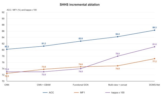
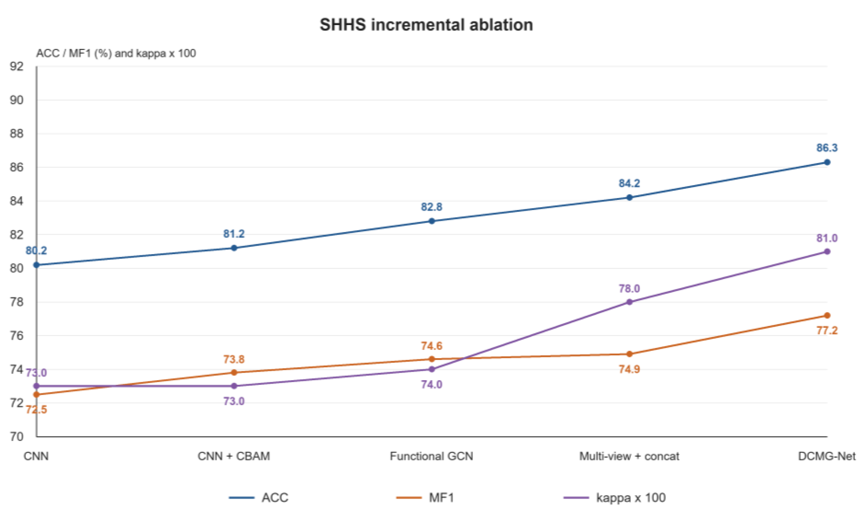
To assess these components with two-channel inputs, the same progression is evaluated on SHHS (Figure 7). The baseline CNN achieves ACC = 80.2%, MF1 = 72.5%, and κ = 0.73. Adding CBAM, functional GCN, and multi-view concatenation increases MF1 to 73.8%, 74.6%, and 74.9%, respectively. The complete model reaches MF1 = 77.2%, ACC = 86.3%, and κ = 0.81. Gating improves MF1 over concatenation and the CNN baseline by 2.3 and 4.7 percentage points. Its advantage over concatenation is consistent with ISRUC-S3, demonstrating the contribution of adaptive fusion under two-channel conditions.

Figure 7. Incremental ablation results on SHHS. ACC and MF1 are percentages; kappa is multiplied by 100 for display.

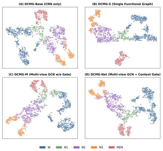
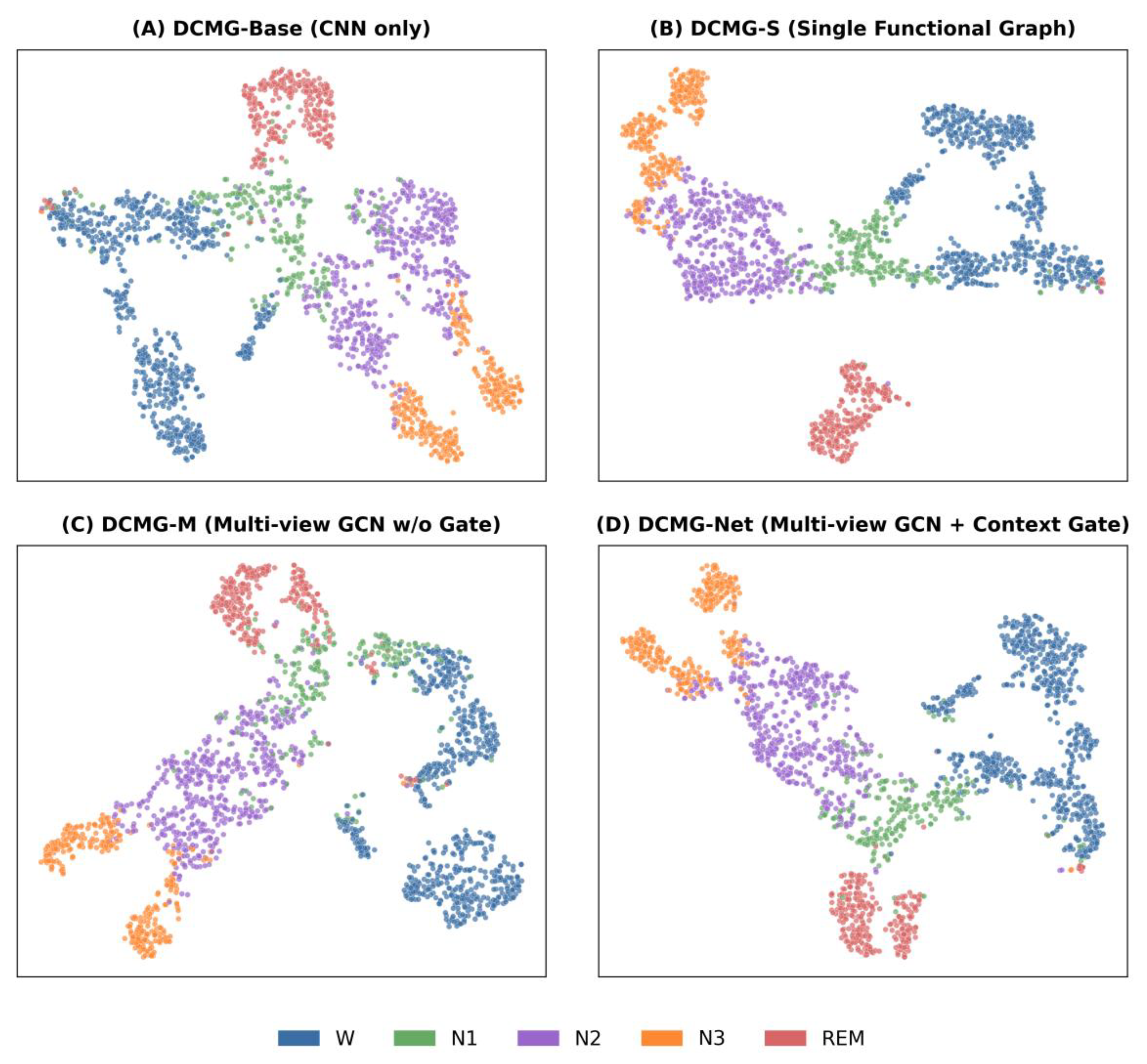
To relate ablation performance to feature distributions, Figure 8 presents two-dimensional t-distributed stochastic neighbor embedding (t-SNE) projections of four model representations. Compared with the baseline CNN, functional-graph and complete gated models show more concentrated class regions and clearer boundaries for some stages. The visualization complements the classification metrics in Figure 6 and Figure 7 by illustrating representation changes after channel aggregation and gated fusion.

Figure 8. Two-dimensional t-SNE visualizations of four model representations, colored by sleep stage.

The incremental ablations examine combinations of modules. To distinguish graph aggregation from general feature transformations, two alternative architectures are evaluated. A six-branch MLP + gating model replaces graph aggregation with nodewise MLPs while retaining six branches and context gating, testing feature mapping without neighborhood propagation. A frequency-aware CNN/attention model directly encodes raw and four band-filtered signals before fusion, comparing direct band-feature encoding with band-relationship modeling. Table 4 reports both alternatives and DCMG-Net on ISRUC-S3 and SHHS, using the same training and evaluation rules within each dataset.

Table 4. Alternative-architecture comparisons on ISRUC-S3 and SHHS.

Dataset	Model	ACC (%)	MF1 (%)	κ
ISRUC-S3	Six-branch MLP + gating	81.6	79.9	0.75
	Frequency-aware CNN/attention	79.3	77.2	0.72
	DCMG-Net (ours)	90.0	88.7	0.87
SHHS	Six-branch MLP + gating	80.7	74.2	0.73
	Frequency-aware CNN/attention	84.1	75.5	0.77
	DCMG-Net (ours)	86.3	77.2	0.81

As shown in Table 4, the six-branch MLP + gating baseline achieves a higher MF1 than the frequency-aware CNN/attention baseline on ISRUC-S3 (79.9% versus 77.2%, a difference of 2.7 percentage points). On SHHS, the ranking reverses: the frequency-aware CNN/attention baseline achieves 75.5%, exceeding the MLP + gating baseline’s 74.2% by 1.3 points. This difference suggests that the relative benefits of direct band-feature encoding and graph-free gated transformations depend on the dataset. DCMG-Net achieves the highest MF1 of the three architectures on both datasets: 88.7% on ISRUC-S3, exceeding the respective baselines by 8.8 and 11.5 points, and 77.2% on SHHS, exceeding them by 3.0 and 1.7 points. These comparisons support graph propagation for jointly encoding channel features and band-specific relationships within the present framework.

To select the reported configuration, feature dimension, gate compression ratio, dropout, focal-loss parameter, and sampling power are further compared on the ISRUC-S3 internal validation set (Table 5). These analyses examine feature capacity, the gating bottleneck, regularization, class-sensitive optimization, and sampling strength, respectively. Candidate settings are compared using internal-validation MF1.

Table 5. Internal-validation hyperparameter results on ISRUC-S3.

Parameter	Values	Validation MF1 (%)
Feature dimension	64/96/128	86.2/85.3/87/88.7
Gate compression ratio	2/4/8	85.7/88.7/87.3
Dropout	0.15/0.25/0.35	86.9/88.7/86.9
Focal γ	0.0/1.2/1.5/2.0	86.4/88.7/86.4/87.1
Sampling power	0.3/0.65/1.0	86.8/88.7/86.1

Within their respective candidate ranges, feature dimension 128, compression ratio 4, dropout 0.25, focal γ = 1.2, and sampling power 0.65 each yield an internal-validation MF1 of 88.7% (Table 5). For γ = 0.0, 1.2, 1.5, and 2.0, MF1 is 86.4%, 88.7%, 86.4%, and 87.1%, respectively, supporting γ = 1.2. These comparisons provide internal-validation evidence for the individual configuration choices. Section 5.8 examines graph construction, preprocessing, augmentation, and context length.

5.8. Graph-Construction and Training Sensitivity

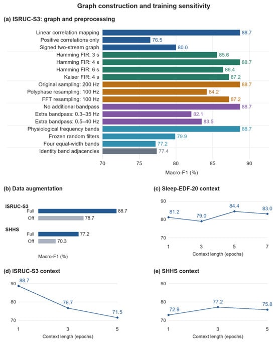
This section examines correlation processing, filtering, resampling, augmentation, and context length. Figure 9 presents MF1 by setting, with augmentation and context results separated by dataset. The context-length panels report internal-validation results used to select the input window before test evaluation. Results are compared within their corresponding groups. Percentage metrics and percentage-point differences are reported to one decimal place; differences are calculated from the displayed values.

Figure 9. Macro-F1 sensitivity: (a) correlation processing, FIR design, resampling, bandpass filtering, and band topology on ISRUC-S3; (b) full augmentation versus no augmentation; (c–e) internal-validation context-length results on Sleep-EDF-20, ISRUC-S3, and SHHS. Percentage values are shown to one decimal place.

Linear correlation mapping, positive correlations only, and separate positive/negative channels yield MF1 values of 88.7%, 76.5%, and 80.0%, respectively. Linear mapping achieves the highest value in this group, exceeding positive-only processing and separate signed channels by 12.2 and 8.7 percentage points. These results support retaining correlation information through linear mapping in this comparison.

Hamming FIR kernels of 3, 4, and 6 s yield MF1 values of 85.6%, 88.7%, and 86.4%, respectively; a 4 s Kaiser kernel yields 87.2%. The 4 s Hamming kernel performs the best among these candidates. Original 200 Hz sampling, polyphase resampling to 100 Hz, and FFT resampling to 100 Hz yield 88.7%, 84.2%, and 87.2%, respectively, favoring the original sampling rate in this comparison. No additional bandpass filtering, additional 0.3–35 Hz filtering, and additional 0.5–40 Hz filtering yield 88.7%, 82.1%, and 83.5%, respectively; the additional filters reduce MF1 by 6.6 and 5.2 percentage points. Physiological bands, frozen random filters, and four equal-width bands yield 88.7%, 79.9%, and 77.2%, respectively. Replacing all four band adjacency matrices with identity matrices yields 77.4%. The physiological-band configuration exceeds these three alternatives by 8.8, 11.5, and 11.3 percentage points, supporting band-specific topology in this comparison.

With full augmentation and no augmentation, ISRUC-S3 MF1 is 88.7% and 78.7%, respectively, a 10.0-percentage-point improvement. On SHHS, the respective values are 77.2% and 70.3%, a 6.9-point improvement. These comparisons indicate that the augmentation pipeline improves classification performance on both datasets.

On the internal validation sets, Sleep-EDF-20 context lengths of 1, 3, 5, and 7 epochs yield MF1 values of 81.2%, 79.0%, 84.4%, and 83.0%, respectively. Five epochs perform best, exceeding one and seven epochs by 3.2 and 1.4 percentage points. For ISRUC-S3, lengths of 1, 3, and 5 yield 88.7%, 76.7%, and 71.5%, respectively, favoring a single epoch. For SHHS, lengths of 1, 3, and 5 yield 72.9%, 77.2%, and 75.8%, respectively. Three epochs exceed one and five epochs by 4.3 and 1.4 points. These validation comparisons determine the dataset-specific lengths before testing and show that increasing context does not improve performance uniformly.

6. Conclusions and Future Work

DCMG-Net unifies multiscale EEG features, band-specific channel topology, and context gating in an end-to-end framework spanning channel encoding, multi-view propagation, and adaptive fusion. Experiments on three public datasets demonstrate effective classification across channel configurations. Incremental ablations further show that gating improves MF1 over direct concatenation by 6.1 percentage points on ISRUC-S3 and 2.3 points on SHHS. The framework provides a reusable approach to jointly exploiting frequency information and channel relationships in EEG-only sleep staging.

Future research will first focus on finer discrimination of transitional stages and interpretation of model mechanisms. Expert annotations of sleep events, including spindles and K-complexes, could support event-guided band representations and adaptive context selection for overlapping N1 and neighboring-stage features. Aligning adjacency and gating responses with sleep events and stage transitions, together with view occlusion and feature interventions, could clarify the contributions of channel relationships and recalibration to predictions.

Beyond the current subject-independent cross-validation, repeated training with multiple seeds, cross-dataset evaluation, and external test sets will examine the effects of sampling rate, channel configuration, and population differences. For portable monitoring, parameter sharing, pruning, and quantization of multi-view encoders and gates will be investigated alongside end-to-end latency, memory use, and power consumption on target hardware. Evaluation with newly acquired signals and computer-assisted scoring workflows will further support the transition from offline assessment to application validation.

References

- Berry, R.B.; Brooks, R.; Gamaldo, C.E.; Harding, S.M.; Marcus, C.L.; Vaughn, B.V.; Tangredi, M.M. The AASM Manual for the Scoring of Sleep and Associated Events: Rules, Terminology and Technical Specifications; American Academy of Sleep Medicine: Darien, IL, USA, 2012. [Google Scholar]
- Silber, M.H.; Ancoli-Israel, S.; Bonnet, M.H.; Chokroverty, S.; Grigg-Damberger, M.M.; Hirshkowitz, M.; Kapen, S.; Keenan, S.A.; Kryger, M.H.; Penzel, T.; et al. The visual scoring of sleep in adults. J. Clin. Sleep Med. 2007, 3, 121–131, Erratum in J. Clin. Sleep Med. 2007, 3, 448. [Google Scholar] [CrossRef] [Scilit]
- Van Der Donckt, J.; Van Der Donckt, J.; Deprost, E.; Vandenbussche, N.; Rademaker, M.; Vandewiele, G.; Van Hoecke, S. Do not sleep on traditional machine learning: Simple and interpretable techniques are competitive to deep learning for sleep scoring. Biomed. Signal Process. Control 2023, 81, 104429. [Google Scholar]
- Jirakittayakorn, N.; Wongsawat, Y.; Mitrirattanakul, S. ZleepAnlystNet: A novel deep learning model for automatic sleep stage scoring based on single-channel raw EEG data using separating training. Sci. Rep. 2024, 14, 9859. [Google Scholar] [CrossRef] [Scilit] [PubMed]
- Li, W.; Gao, J. Automatic sleep staging by a hybrid model based on deep 1D-ResNet-SE and LSTM with single-channel raw EEG signals. PeerJ Comput. Sci. 2023, 9, e1561. [Google Scholar] [CrossRef] [Scilit] [PubMed]
- Supratak, A.; Dong, H.; Wu, C.; Guo, Y. DeepSleepNet: A model for automatic sleep stage scoring based on raw single-channel EEG. IEEE Trans. Neural Syst. Rehabil. Eng. 2017, 25, 1998–2008. [Google Scholar] [CrossRef] [Scilit] [PubMed]
- Perslev, M.; Jensen, M.; Darkner, S.; Jennum, P.J.; Igel, C. U-Time: A fully convolutional network for time series segmentation applied to sleep staging. In Advances in Neural Information Processing Systems 32 (NIPS 2019), Proceedings of the 33rd Conference on Neural Information Processing Systems (NeurIPS 2019), Vancouver, BC, Canada, 8–14 December 2019; Curran Associates, Inc.: Red Hook, NY, USA, 2019; Volume 32, Available online: https://proceedings.neurips.cc/paper_files/paper/2019/hash/57bafb2c2dfeefba931bb03a835b1fa9-Abstract.html (accessed on 1 March 2025).
- Goshtasbi, N.; Boostani, R.; Sanei, S. SleepFCN: A fully convolutional deep learning framework for sleep stage classification using single-channel electroencephalograms. IEEE Trans. Neural Syst. Rehabil. Eng. 2022, 30, 2088–2096. [Google Scholar] [CrossRef] [Scilit] [PubMed]
- Dai, Y.; Li, X.; Liang, S.; Wang, L.; Duan, Q.; Yang, H.; Zhang, C.; Chen, X.; Li, L.; Li, X.; et al. MultiChannelSleepNet: A Transformer-based model for automatic sleep stage classification with PSG. IEEE J. Biomed. Health Inform. 2023, 27, 4204–4215. [Google Scholar] [CrossRef] [Scilit] [PubMed]
- Eldele, E.; Chen, Z.; Liu, C.; Wu, M.; Kwoh, C.-K.; Li, X.; Guan, C. An attention-based deep learning approach for sleep stage classification with single-channel EEG. IEEE Trans. Neural Syst. Rehabil. Eng. 2021, 29, 809–818. [Google Scholar] [CrossRef] [Scilit] [PubMed]
- Jia, Z.; Lin, Y.; Wang, J.; Zhou, R.; Ning, X.; He, Y.; Zhao, Y. GraphSleepNet: Adaptive spatial-temporal graph convolutional networks for sleep stage classification. In Proceedings of the Twenty-Ninth International Joint Conference on Artificial Intelligence, IJCAI, Virtual, 7–15 January 2021; pp. 1324–1330. [Google Scholar] [CrossRef] [Scilit] [PubMed]
- Einizade, A.; Nasiri, S.; Sardouie, S.H.; Clifford, G.D. ProductGraphSleepNet: Sleep staging using product spatio-temporal graph learning with attentive temporal aggregation. Neural Netw. 2023, 164, 667–680. [Google Scholar] [CrossRef] [Scilit] [PubMed]
- Li, Y.; Chen, J.; Ma, W.; Zhao, G.; Fan, X. MVF-SleepNet: Multi-view fusion network for sleep stage classification. IEEE J. Biomed. Health Inform. 2024, 28, 2485–2495. [Google Scholar] [CrossRef] [Scilit] [PubMed]
- Yang, J.; Wang, Q.; Dong, X.; Shen, T. Synergistic integration of brain networks and time-frequency multi-view feature for sleep stage classification. Health Inf. Sci. Syst. 2025, 13, 15. [Google Scholar] [CrossRef] [Scilit] [PubMed]
- Purcell, S.M.; Manoach, D.S.; Demanuele, C.; Cade, B.; Mariani, S.; Cox, R.; Panagiotaropoulou, G.; Saxena, R.; Pan, J.Q.; Smoller, J.W.; et al. Characterizing sleep spindles in 11,630 individuals from the National Sleep Research Resource. Nat. Commun. 2017, 8, 15930. [Google Scholar] [CrossRef] [Scilit] [PubMed]
- Li, H.; Zhang, X.; Guo, K. MFST-GCN: A sleep stage classification method based on multi-feature spatio-temporal graph convolutional network. Brain Sci. 2026, 16, 162. [Google Scholar] [CrossRef] [Scilit] [PubMed]
- Wang, K.; Yue, H.; Chen, Z.; Ma, W. SSL-MSTFNet: A multi-scale temporal-spectral fusion network with self-supervision learning for sleep stage classification. In Advanced Data Mining and Applications, Proceedings of the 21st International Conference, ADMA 2025, Kyoto, Japan, 22–24 October 2025; Yoshikawa, M., Meng, X., Cao, Y., Xiao, C., Chen, W., Wang, Y., Eds.; Springer: Singapore, 2026; Volume 16198. [Google Scholar] [CrossRef] [Scilit]
- Fang, Y.; Xia, Y.; Chen, P.; Zhang, J.; Zhang, Y. A dual-stream deep neural network integrated with adaptive boosting for sleep staging. Biomed. Signal Process. Control 2023, 79, 104150. [Google Scholar] [CrossRef] [Scilit]
- Miech, A.; Laptev, I.; Sivic, J. Learnable pooling with context gating for video classification. arXiv 2017, arXiv:1706.06905. [Google Scholar] [CrossRef] [Scilit]
- Woo, S.; Park, J.; Lee, J.-Y.; Kweon, I.S. CBAM: Convolutional block attention module. In Proceedings of the European Conference on Computer Vision (ECCV), Munich, Germany, 8–14 September 2018. [Google Scholar]
- Kipf, T.N.; Welling, M. Semi-supervised classification with graph convolutional networks. arXiv 2016, arXiv:1609.02907. [Google Scholar] [CrossRef] [Scilit]
- Fiorillo, L.; Puiatti, A.; Papandrea, M.; Ratti, P.-L.; Favaro, P.; Roth, C.; Bargiotas, P.; Bassetti, C.L.; Faraci, F.D. Automated sleep scoring: A review of the latest approaches. Sleep Med. Rev. 2019, 48, 101204. [Google Scholar] [CrossRef] [Scilit] [PubMed]
- Zhang, W.; Li, C.; Peng, H.; Qiao, H.; Chen, X. CTCNet: A CNN Transformer capsule network for sleep stage classification. Measurement 2024, 226, 114157. [Google Scholar] [CrossRef] [Scilit]
- Li, T.; Gong, Y.; Chen, X. TransUSleepNet: A scalable multi-modal U-shaped sleep rating learning architecture based on xLSTM and Transformer. IAENG Int. J. Comput. Sci. 2026, 53, 1625–1636. [Google Scholar]
- Fox, B.; Jiang, J.; Wickramaratne, S.; Kovatch, P.; Suarez-Farinas, M.; Shah, N.A.; Parekh, A.; Nadkarni, G.N. A foundational transformer leveraging full night, multichannel sleep study data accurately classifies sleep stages. Sleep 2025, 48, zsaf061. [Google Scholar] [CrossRef] [Scilit] [PubMed]
- Klein, T.; Minakowski, P.; Sager, S. Flexible Patched Brain Transformer model for EEG decoding. Sci. Rep. 2025, 15, 10935. [Google Scholar] [CrossRef] [Scilit] [PubMed]
- Wang, C.; Hou, Z.; Gao, J.; Zhong, X.; Han, S.; Zhang, T. LGFNet: A CTC-guided local-global fusion framework for single-channel sleep staging. arXiv 2026, arXiv:2607.25197. [Google Scholar] [CrossRef] [Scilit]
- Phan, H.; Andreotti, F.; Cooray, N.; Chen, O.Y.; De Vos, M. SeqSleepNet: End-to-end hierarchical recurrent neural network for sequence-to-sequence automatic sleep staging. IEEE Trans. Neural Syst. Rehabil. Eng. 2019, 27, 400–410. [Google Scholar] [CrossRef] [Scilit] [PubMed]
- Jia, Z.; Lin, Y.; Wang, J.; Ning, X.; He, Y.; Zhou, R.; Zhou, Y.; Lehman, L.-W.H. Multi-view spatial-temporal graph convolutional networks with domain generalization for sleep stage classification. IEEE Trans. Neural Syst. Rehabil. Eng. 2021, 29, 1977–1986. [Google Scholar] [CrossRef] [Scilit] [PubMed]
- An, P.; Zhao, J.; Du, B.; Zhao, W.; Zhang, T.; Yuan, Z. Amplitude–time dual-view fused EEG temporal feature learning for automatic sleep staging. IEEE Trans. Neural Netw. Learn. Syst. 2022, 35, 6492–6506. [Google Scholar] [CrossRef] [Scilit] [PubMed]
- Goerttler, S.; Wang, Y.; Eldele, E.; He, F.; Wu, M. MSA-CNN: A lightweight multi-scale CNN with attention for sleep stage classification. Biomed. Signal Process. Control 2026, 120, 110141. [Google Scholar] [CrossRef] [Scilit]
- Phan, H.; Chen, O.Y.; Tran, M.C.; Koch, P.; Mertins, A.; De Vos, M. XSleepNet: Multi-view sequential model for automatic sleep staging. IEEE Trans. Pattern Anal. Mach. Intell. 2021, 44, 5903–5915. [Google Scholar] [CrossRef] [Scilit] [PubMed]
- Wang, X.; Zhu, Y.; Lai, W. MIASS: A multi-interactive attention model for sleep staging via EEG and EOG signals. Comput. Electr. Eng. 2025, 121, 109852. [Google Scholar] [CrossRef] [Scilit]
- Yu, T.; Hu, X.; He, Y.; Wu, W.; Gu, Z.; Yu, Z.; Li, Y.; Wang, F.; Xiao, J. Multi-view self-supervised learning enhances automatic sleep staging from EEG signals. IEEE Trans. Biomed. Eng. 2025, 72, 3056–3070. [Google Scholar] [CrossRef] [Scilit] [PubMed]
- Demir, A.; Koike-Akino, T.; Wang, Y.; Haruna, M.; Erdogmus, D. EEG-GNN: Graph neural networks for classification of electroencephalogram (EEG) signals. In Proceedings of the 43rd Annual International Conference of the IEEE Engineering in Medicine and Biology Society (EMBC), Virtual, 1–5 November 2021. [Google Scholar]
- Ma, J.; Lv, X.; Zhang, Y. MFSleepNet: A multi-receptive field sleep networks for sleep stage classification. Biomed. Signal Process. Control 2025, 102, 107264. [Google Scholar] [CrossRef] [Scilit]
- Chen, J.; Dai, Y.; Chen, X.; Shen, Y.; Luximon, Y.; Wang, H.; He, Y.; Ma, W.; Fan, X. StAGN: Spatial-temporal adaptive graph network via contrastive learning for sleep stage classification. In Proceedings of the SIAM International Conference on Data Mining (SDM), Minneapolis, MN, USA, 27–29 April 2023. [Google Scholar]
- Anderer, P.; Roberts, S.; Schlögl, A.; Gruber, G.; Klösch, G.; Herrmann, W.; Rappelsberger, P.; Filz, O.; Barbanoj, M.J.; Dorffner, G.; et al. Artifact processing in computerized analysis of sleep EEG–a review. Neuropsychobiology 1999, 40, 150–157. [Google Scholar] [CrossRef] [Scilit] [PubMed]
- Steriade, M. Corticothalamic resonance, states of vigilance and mentation. Neuroscience 2000, 101, 243–276. [Google Scholar] [CrossRef] [Scilit] [PubMed]
- Li, Q.; Han, Z.; Wu, X.-M. Deeper insights into graph convolutional networks for semi-supervised learning. In Proceedings of the AAAI Conference on Artificial Intelligence, New Orleans, LA, USA, 2–7 February 2018; Volume 32. [Google Scholar]
- Khalighi, S.; Sousa, T.; Santos, J.M.; Nunes, U. ISRUC-Sleep: A comprehensive public dataset for sleep researchers. Comput. Methods Programs Biomed. 2016, 124, 180–192. [Google Scholar] [CrossRef] [Scilit] [PubMed]
- Quan, S.F.; Howard, B.V.; Iber, C.; Kiley, J.P.; Nieto, F.J.; O’Connor, G.T.; Rapoport, D.M.; Redline, S.; Robbins, J.; Samet, J.M.; et al. The Sleep Heart Health Study: Design, rationale, and methods. Sleep 1997, 20, 1077–1085. [Google Scholar] [CrossRef] [Scilit]
- Kemp, B.; Zwinderman, A.; Tuk, B.; Kamphuisen, H.; Oberye, J. Analysis of a sleep-dependent neuronal feedback loop: The slow-wave microcontinuity of the EEG. IEEE Trans. Biomed. Eng. 2000, 47, 1185–1194. [Google Scholar] [CrossRef] [Scilit] [PubMed]
- Lin, T.-Y.; Goyal, P.; Girshick, R.; He, K.; Dollar, P. Focal loss for dense object detection. In Proceedings of the IEEE International Conference on Computer Vision (ICCV), Venice, Italy, 22–29 October 2017. [Google Scholar]
- Loshchilov, I.; Hutter, F. Decoupled weight decay regularization. arXiv 2017, arXiv:1711.05101. [Google Scholar] [CrossRef] [Scilit]
- Goldberger, A.L.; Amaral, L.A.N.; Glass, L.; Hausdorff, J.M.; Ivanov, P.C.; Mark, R.G.; Mietus, J.E.; Moody, G.B.; Peng, C.-K.; Stanley, H.E. PhysioBank, PhysioToolkit, and PhysioNet: Components of a new research resource for complex physiologic signals. Circulation 2000, 101, e215–e220. [Google Scholar] [PubMed]
- Phan, H.; Chen, O.Y.; Koch, P.; Lu, Z.; McLoughlin, I.; Mertins, A.; De Vos, M. Towards more accurate automatic sleep staging via deep transfer learning. IEEE Trans. Biomed. Eng. 2020, 68, 1787–1798. [Google Scholar] [CrossRef] [Scilit] [PubMed]
- Paisarnsrisomsuk, S.; Ruiz, C.; Alvarez, S.A. Capturing the development of internal representations in a high-performing deep network for sleep stage classification. SN Comput. Sci. 2021, 2, 318. [Google Scholar] [CrossRef] [Scilit]
- Zhou, W.; Zhu, H.; Shen, N.; Chen, H.; Fu, C.; Yu, H.; Shu, F.; Chen, C.; Chen, W. A lightweight segmented attention network for sleep staging by fusing local characteristics and adjacent information. IEEE Trans. Neural Syst. Rehabil. Eng. 2022, 31, 238–247. [Google Scholar] [CrossRef] [Scilit] [PubMed]
- Mousavi, S.; Afghah, F.; Acharya, U.R. SleepEEGNet: Automated sleep stage scoring with sequence to sequence deep learning approach. PLoS ONE 2019, 14, e0216456. [Google Scholar] [CrossRef]
- Sun, Y.; Wang, B.; Jin, J.; Wang, X. Deep convolutional network method for automatic sleep stage classification based on neurophysiological signals. In Proceedings of the 11th International Congress on Image and Signal Processing, BioMedical Engineering and Informatics (CISP-BMEI), Beijing, China, 13–15 October 2018; pp. 1–5. [Google Scholar]
- Phan, H.; Andreotti, F.; Cooray, N.; Chén, O.Y.; de Vos, M. Joint classification and prediction CNN framework for automatic sleep stage classification. IEEE Trans. Biomed. Eng. 2019, 66, 1285–1296. [Google Scholar] [CrossRef] [Scilit] [PubMed]
- Fei, K.; Wang, J.; Pan, L.; Wang, X.; Chen, B. A sleep staging model on wavelet-based adaptive spectrogram reconstruction and light weight CNN. Comput. Biol. Med. 2024, 173, 108300. [Google Scholar] [CrossRef] [Scilit] [PubMed]
- Huang, P.; Qiu, M.; Liu, Y.; Fan, X. Advancing sleep stages classification through a dual-Graphormer approach. Expert Syst. Appl. 2025, 288, 128220. [Google Scholar] [CrossRef] [Scilit]
- Yang, Z.; Qiu, M.; Fan, X.; Dai, G.; Ma, W.; Peng, X.; Fu, X.; Li, Y. CVAN: A novel sleep staging method via cross-view alignment network. IEEE J. Biomed. Health Inform. 2025, 29, 4659–4671. [Google Scholar] [CrossRef] [Scilit] [PubMed]
- Pei, W.; Li, Y.; Wen, P.; Yang, F.; Ji, X. An automatic method using MFCC features for sleep stage classification. Brain Inform. 2024, 11, 6. [Google Scholar] [CrossRef] [Scilit] [PubMed]
- Wang, W.; Xiao, Q.; Xue, J.; Hu, Z. DynamicSleepNet: A multi-exit neural network with adaptive inference time for sleep stage classification. Front. Physiol. 2023, 14, 1171467. [Google Scholar] [CrossRef] [Scilit] [PubMed]
- Jia, Z.; Cai, X.; Zheng, G.; Wang, J.; Lin, Y. SleepPrintNet: A multivariate multimodal neural network based on physiological time-series for automatic sleep staging. IEEE Trans. Artif. Intell. 2021, 1, 248–257. [Google Scholar] [CrossRef] [Scilit]
- Wang, Y.; Wu, M.; Li, X.; Xie, L.; Chen, Z. Multivariate time series representation learning via hierarchical correlation pooling boosted graph neural network. IEEE Trans. Artif. Intell. 2023, 5, 321–333. [Google Scholar] [CrossRef] [Scilit]
- Wang, Y.; Xu, Y.; Yang, J.; Wu, M.; Li, X.; Xie, L.; Chen, Z. Fully connected spatial-temporal graph for multivariate time-series data. Proc. AAAI Conf. Artif. Intell. 2024, 38, 15715–15724. [Google Scholar] [CrossRef] [Scilit]
Disclaimer/Publisher’s Note: The statements, opinions and data contained in all publications are solely those of the individual author(s) and contributor(s) and not of MDPI and/or the editor(s). MDPI and/or the editor(s) disclaim responsibility for any injury to people or property resulting from any ideas, methods, instructions or products referred to in the content. |
© 2026 by the authors. Licensee MDPI, Basel, Switzerland. This article is an open access article distributed under the terms and conditions of the Creative Commons Attribution (CC BY) license.