Which Local Search Operator Works Best for the Open-Loop TSP?

Abstract

The traveling salesman problem (TSP) has been widely studied for the classical closed-loop variant. However, very little attention has been paid to the open-loop variant. Most of the existing studies also focus merely on presenting the overall optimization results (gap) or focus on processing time, but do not reveal much about which operators are more efficient to achieve the result. In this paper, we present two new operators (link swap and 3–permute) and study their efficiency against existing operators, both analytically and experimentally. Results show that while 2-opt and relocate contribute equally in the closed-loop case, the situation changes dramatically in the open-loop case where the new operator, link swap, dominates the search; it contributes by 50% to all improvements, while 2-opt and relocate have a 25% share each. The results are also generalized to tabu search and simulated annealing.

1. Introduction

The traveling salesman problem (TSP) aims to find the shortest tour for a salesperson to visit N number of cities. In graph theory, a cycle including every vertex of a graph makes a Hamiltonian cycle. Therefore, in the context of graph theory, the solution to a TSP is defined as the minimum-weight Hamiltonian cycle in a weighted graph. In this paper, we consider the symmetric Euclidean TSP variant, where the distance between two cities is calculated by their distance in the Euclidean space. Both the original problem [1] and its Euclidean variant are NP–hard [2]. Finding the optimum solution efficiently is therefore not realistic, even for the relatively small size of the input.

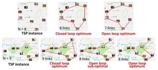
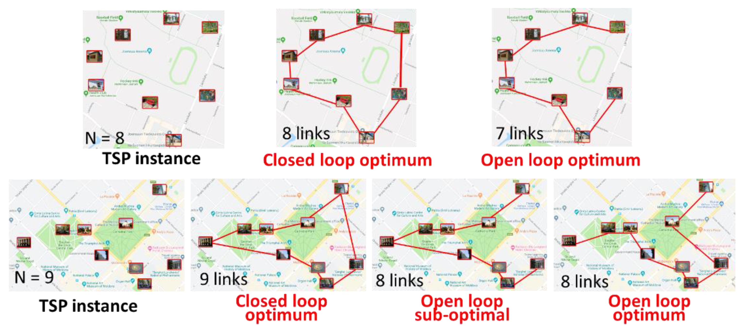
O–Mopsi (http://cs.uef.fi/o-mopsi/) is a mobile-based orienteering game where the player needs to find some real-world targets, with the help of GPS navigation [3]. Unlike a prior instruction of visiting order in the classical orienteering, O–Mopsi players have to decide the order of visiting targets by themselves. The game finishes immediately when the last target is reached. The player does not need to return to the start target. This corresponds to a special case of the orienteering problem [4]. Finding the optimum order by minimizing the tour length corresponds to solving open-loop TSP [5], because the players are not required to return to the start position. The open-loop variant is also NP–hard [2]. The solution to a closed-loop TSP is a tour; however, the solution to an open-loop TSP is an open path. Hence, a TSP with the size N contains N links in its closed-loop solution and N-1 in its open-loop solution (Figure 1). However, the optimum solution to an open-loop TSP is not usually achievable by removing the largest link from the optimum solution to the closed-loop TSP (Figure 1).

Figure 1. Difference between open- and closed-loop traveling salesman problem (TSP).

In O–Mopsi, players are not required to solve the optimum tour, but finding a good tour is still an essential part of the game. Experiments showed that, among the players who completed a game, only 14% had found the optimum tour, even if the number of targets was about 10, on average [3]. The optimum tour is still needed for reference when analyzing the performance of the players. This is usually made as a post-game analysis but can also happen during real-time play. A comparison can be made with the tour length or with the visiting order. The game creator also needs an estimator for the tour length, as it will be published as a part of the game info. If the game is created automatically on the demand, TSP must be solved real-time. The optimality is highly desired, but can sometimes be compromised for the sake of fast processing.

The number of targets in the current O–Mopsi instances varies from 4 to 27, but larger instances may appear. For the smaller instances, the relatively simple branch-and-bound algorithm is fast enough to produce the optimum tour. However, for the longer instances, it might take from minutes to hours. Along with the exact solver, a faster heuristic algorithm is therefore needed to find the solution more quickly, in spite of the danger of occasionally resulting in a sub-optimal solution. Besides O–Mopsi, TSP arises in route planning [6], orienteering problems [7], and automated map generation [8].

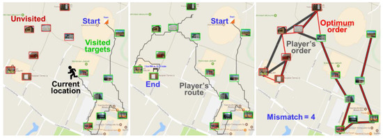
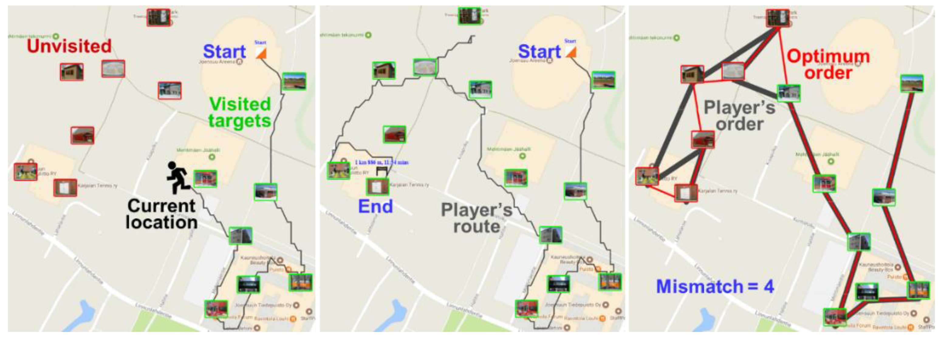
An example of O–Mopsi play is shown in Figure 2, with a comparison to the optimum tour (reference). For analyzing, we calculate several reference tours: optimum, fixed-start, and dynamic. The optimum tour takes into account the fact that the players can freely choose their starting point. Since selecting the best starting point is challenging [9], we also calculate two alternative reference tours from the location where the player started. Fixed-start is the optimum tour using this starting point. The dynamic tour follows the player’s choices from the starting point but re-calculates the new optimum every time the player deviates from optimum path. Three different evaluation measures are obtained using these three tours: gap, mismatches, and mistakes; see [10].

Figure 2. Examples of O–Mopsi playing (left), the final tour (middle) and comparison to optimum tour (right).

Being NP–hard, exact solvers of TSPs are time-consuming. Despite the huge time consumption, exact solvers were prime attractions to researchers in earlier days. Dantzig, Fulkerson, and Johnson [11], Held and Karp [12], Padberg and Rinaldi [13], Grötschel and Holland [14], Applegate et al. [15], and others developed different algorithms to produce exact solutions. Laporte [16] surveyed exact algorithms for TSP. By the year 2006, the Concorde solver solved a TSP instance with 85900 cities [17].

Along with these, different heuristic algorithms have been developed to find very fast near-optimal solutions. The local search is one of the most common heuristics to produce near-optimum results [18]. It has two parts: tour construction and tour improvement. The tour construction generates an initial solution that can be far beyond the optimum. A significant amount of research developed different tour construction algorithms, such as the savings algorithm by Reference [19], polynomial–time 3/2 approximation algorithm by Reference [20], insertion [21], greedy [21], and the nearest neighbor algorithm [21]. Among these, we use the greedy algorithm and a random arrangement for the tour construction.

Being an iterative process, the tour improvement step modifies the initial solution with a small improvement in each iteration. The key component in the local search is the choice of the operator, which defines how the current solution is modified to generate new candidate solutions. Most used operators are 2-opt [22] and its generalized variant, called k–opt [23], which is empirically the most effective local search algorithm for large TSPs [24]. Okano et al. [25] analyzed the combination of 2-opt with different well-known construction heuristics. Several researchers studied local search for TSP and different optimization problems [16,21,26,27,28,29,30,31,32], even for vehicle routing application [33,34].

Although existing studies have analyzed the local search algorithms extensively, it is still not known which operators are effective for open-loop cases. Besides this, the existing literature mainly presents optimization results of algorithms instead of providing a detailed study on different operators. As operators are the backbone of the local search algorithms, we need a detailed study on them to know how to increase the productivity of the algorithm and how to avoid the local minima.

In this paper, we study several operators and their combinations in the context of local search. We aim at answering which of them works best in terms of the quality and efficiency. We consider four operations, of which two are existing and two are new:

• Relocate [35]
• 2-opt [22]
• 3–permutation (new)
• Link swap (new)

Between the new two operators, the former also applies to the more common closed-loop TSP, but the second is specifically tailored for the open-loop problem. We also propose an algorithm to achieve a global minimum in most problem instances of size up to 31, preferably in real-time.

We study the performance of these operators when applied separately, and when mixed. We consider random, best improvement, and first improvement search strategies. We first report how successful the operators are in equal conditions, and whether the choice of the best operator changes towards the end of the iterations. We study two initialization techniques: random and heuristic, and the effect of re-starting the search. Results are reported for two open-loop datasets (O–Mopsi, Dots), see Table 1. The O–Mopsi dataset contains real-world TSP instances and the Dots dataset is a computer-generated random dataset for an experimental computer game. Since it is an outdoor dataset, generating the former one is relatively difficult. Therefore, the available number of instances are much lower than Dots. However, both datasets need real-time reference solutions.

Table 1. Datasets used in this study.

Dataset:	Type:	Distance:	Instances:	Sizes:
O-Mopsi 1	Open loop	Haversine	145	4-27
Dots 1	Open loop	Euclidean	4226	4-31

¹http://cs.uef.fi/o-mopsi/datasets/.

The rest of the paper is organized as follows. In Section 2, we describe the local search operators we use in this study. We define these operators with illustrations and study their abilities to produce unique improved solutions. In Section 3, we provide results of the tests carried on with these operators on Table 1 datasets. Based on these results, we introduce a new method to solve open-loop TSPs in this section. In Section 4, we evaluate the quality and efficiency of our proposed algorithm. In Section 5, we test stochastic variants, aiming to improve our algorithm. Lastly, in Section 6, we conclude our findings in this study.

2. Local Search

The local search is a way to upgrade an existing solution to a new candidate solution by small changes. A local search operator seeks and finds a small modification to improve the solution. The search approach of a local search operator can be one of several of different types. In the first and best improvement strategy, the first and best candidate is always chosen among all the candidates, respectively. For these two cases, we continue the search until saturation, which means no further improvement is found. In a random search strategy, candidates are chosen randomly until some constant iteration. In the local search, a better solution can almost always be found.

We next study the following four operators:

• Relocate [35]
• 2-opt [22]
• 3–permute (new)
  Link swap (new)

2.1. Relocate

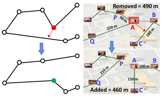
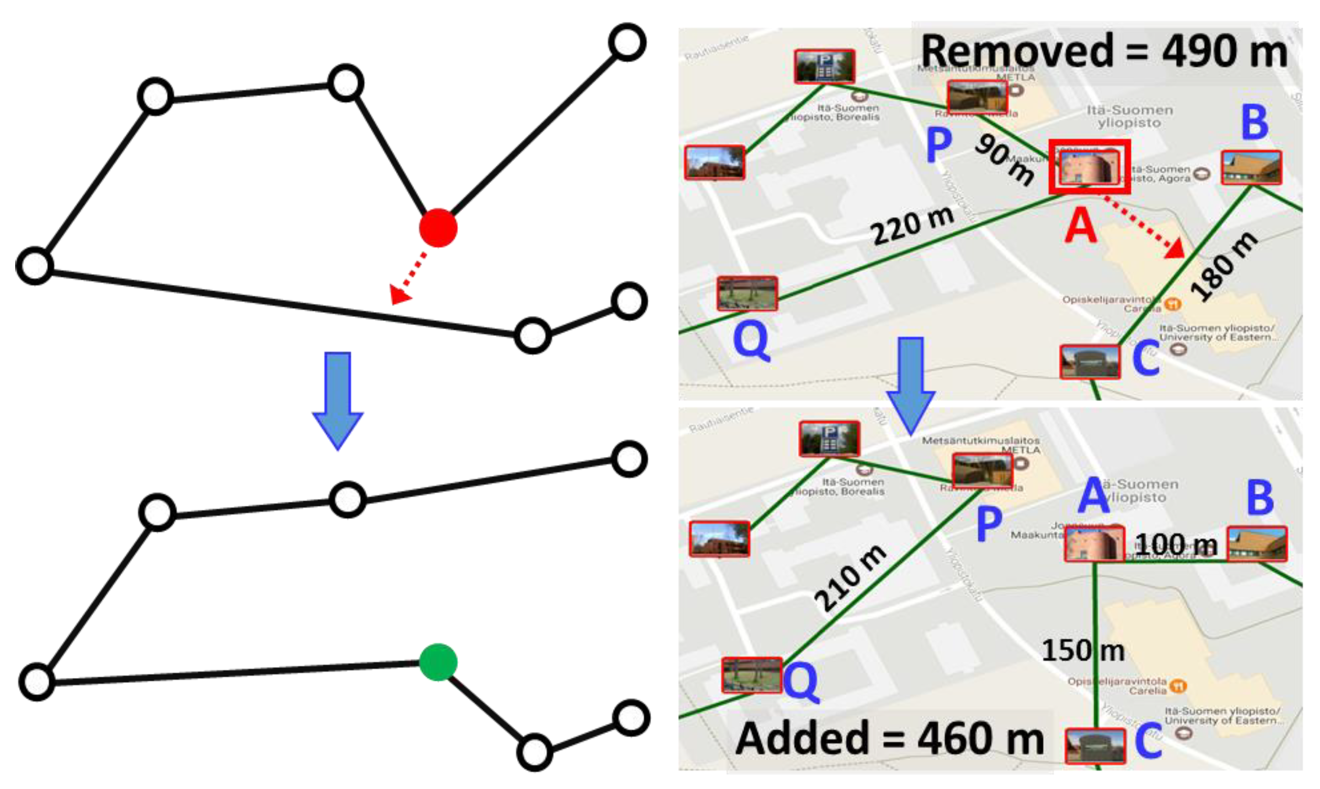
Changing the order of nodes can produce different solutions. Relocate is the process where a selected node (target) is moved from its current position in the tour to another position (destination). Hence, the position of the selected node is relocated. Each relocation of a node produces one outcome. Gendreau, Hertz, and Laporte [35] developed the GENI method to insert a new node by breaking a link. We use this idea and create relocate as a tour improvement operator. Figure 3 illustrates relocate using an O-Mopsi example, where target A is moved between B and C. First, we take A from its current position by removing links PA and AQ, and by adding link PQ to close the gap. Then, A is added to its new position by removing link BC, and by adding BA and AC. As an effect, the tour becomes 30 m shorter. The size of the search neighborhood is O(N²) because there are N possible targets and N-2 destinations to choose from, in total.

Figure 3. Working of the relocate operator and an example of how it improves the tour in an O–Mopsi game by 30 meters.

2.2. Two-Optimization (2-opt)

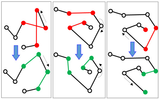
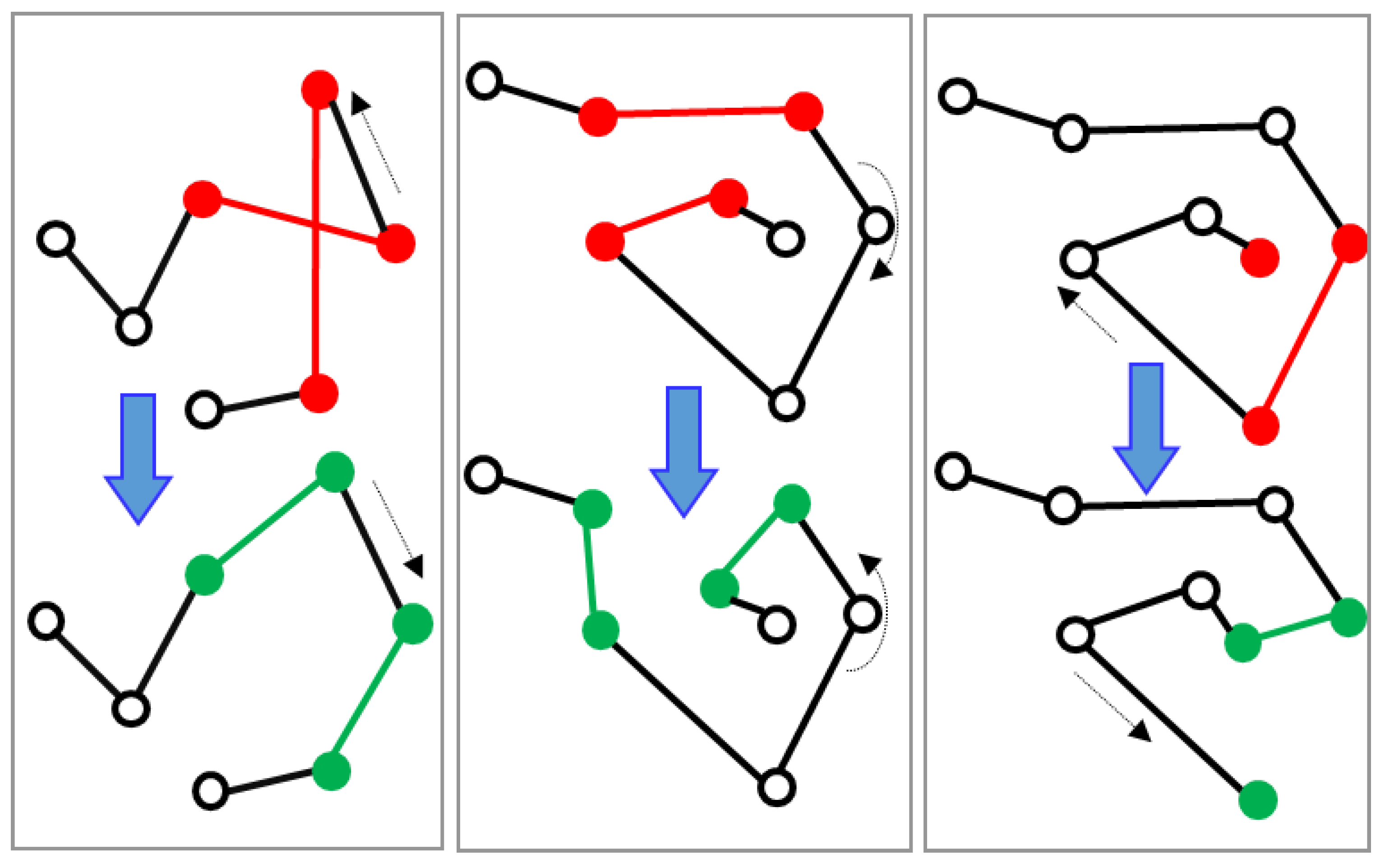
Croes [22] first introduced the 2-optimization method, which is a simple and very common operator [36]. The idea of 2-opt is to exchange the links between two pairs of subsequent nodes as shown in Figure 4. It has also been generalized to k–opt (L–K heuristics) [23] and implemented by Helsgaun [37]. Johnson and McGeoch [21] explained thoroughly the 2-opt and 3–opt processes. In the case of 3–opt, the only difference from 2-opt is to exchange the links between three pairs of nodes. The method was originally developed for the closed-loop TSP, but it applies to the open-loop TSP as well. In addition, we also consider dummy nodes paired with one of the two terminal nodes. Such a way, terminal nodes can also change into an internal node.

Figure 4. Three examples of how the 2-optimization method can improve the tour.

The 2-opt approach removes crossings in the path. Pan and Xia [38] highlighted this cross-removing effect in their work. However, 2-opt is more than the cross-removal method, as shown in Figure 4.

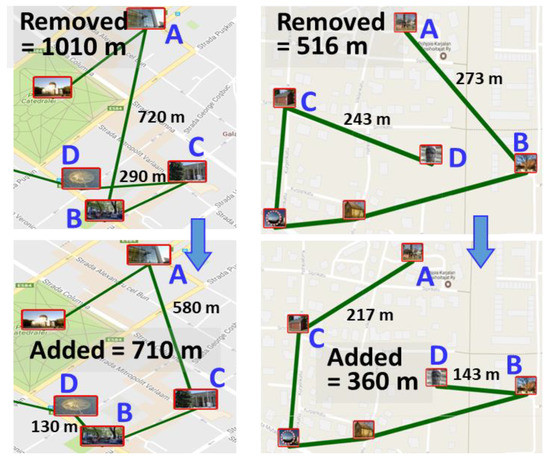
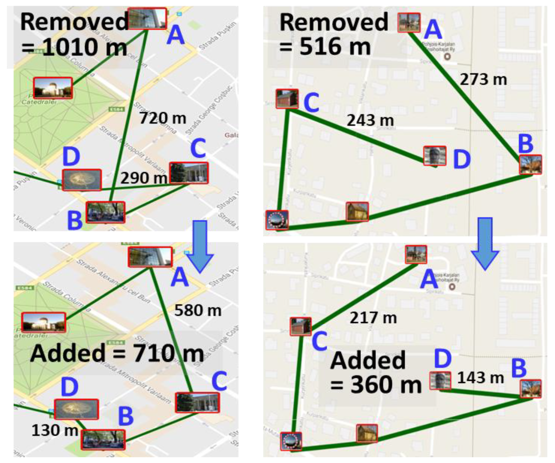
In Figure 5, 2-opt is illustrated with two real examples from O-Mopsi. Here, AB and CD are the two links involved in the operation. In the modified tour, these links are replaced by AC and BD. In the first example, the original links cross, which is then deleted and the length of the overall tour is shortened from 1010 m to 710 m. The second example shows that 2-opt can also improve the tour, even when the original links do not cross.

Figure 5. Two examples of the 2-opt method in O-Mopsi.

The 2-opt operator works with links. A tour consists of N-1 links, so there are (N-1)*(N-2) possible pairs of links. Thus, the size of the neighborhood is O(N²).

2.3. Three-Node Permutation (3-permute)

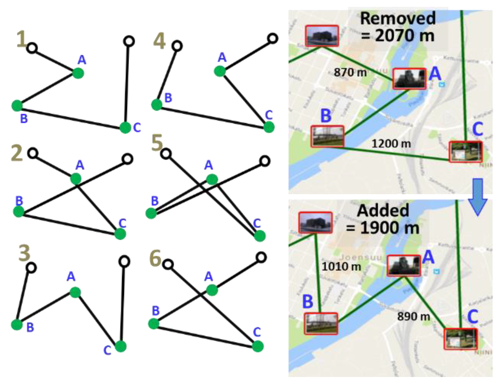
Permutation between the order of the nodes is another potentially useful operator for the local search. Although the idea is quite straightforward, we are not aware of its existence in literature, so we will briefly consider it here. As per the theory, three nodes (A, B, C) can generate six different orders. Therefore, given an existing sequence (triple) of three nodes, ABC, we can create five new solutions: ACB, BAC, BCA, CAB, and CBA.

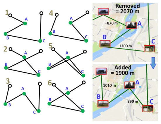
In Figure 6, an original and its five alternatives are shown. The real O-Mopsi game where this example originates from is also shown. Here, the tour length is reduced by 170 m when changing the original order (ABC) to the better one (BAC).

Figure 6. All six combinations of 3–permute and an O–Mopsi game example that is improved by 170 m.

There are N-1 possible triples, including two dummies after the terminal points. The size of the neighborhood is, therefore, 6*(N-1) = O(N), which is significantly smaller than that of the relocate and 2-opt operators.

2.4. Link Swap

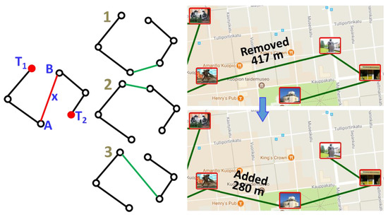
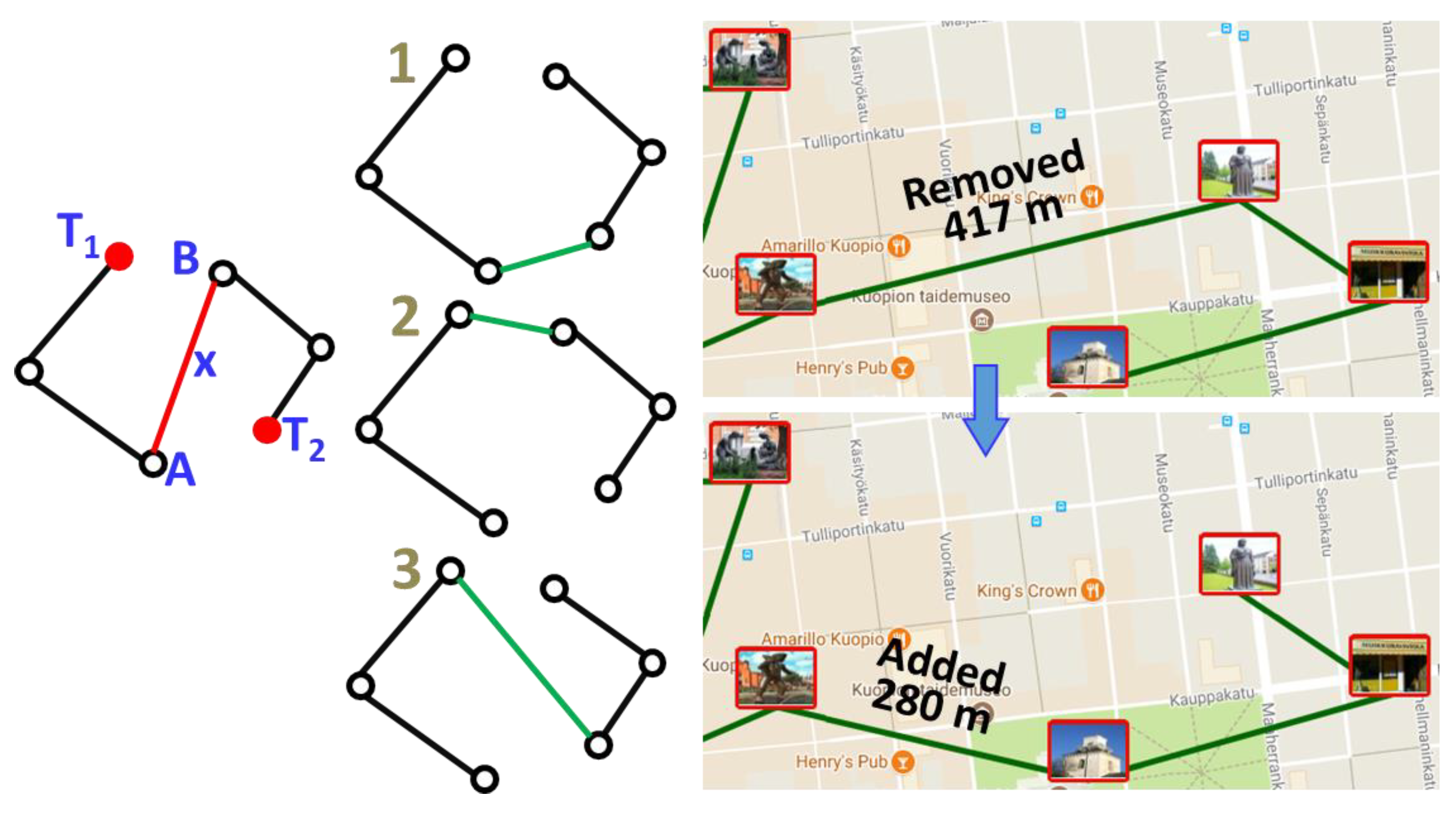
Solving the open-loop variant of TSP allows us to introduce a new operator that is not possible with the closed-loop problem. Link swap is analogous to relocate, hence we consider one link, AB, and swap it into a new location in the tour, see Figure 7. However, to keep the new solution as a valid TSP tour, we are limited to three choices: replace AB by AT₂, BT₁, or T₁T₂. As a result, one or both of the nodes A and B will become a new terminal node.

Figure 7. Original tour and three alternatives created by link swap (left). In each case, the link x is replaced by a new link connecting to one or both terminal nodes. In the O–Mopsi example (right), the tour is improved by 137m.

In the O–Mopsi example in Figure 7, we can see that a single link swap operation improves the solution by reducing the tour length up to 137 m.

We have N–1 choices for a link to be removed, and for each of them, we have three new alternatives. Thus, the size of the neighborhood is 3*(N–1) = O(N). Link swap is a special case of 3–opt and relocate operator, but as the size of the neighborhood is linear, it is a faster operation than both 3–opt and relocate operator.

2.5. The Uniqueness of the Operators

All operators create a large number of neighbor solutions. The set of solutions generated by one operator can be similar to the set of another operator. Given the same initial solution, if all the candidate solutions generated by one operator were a subset of the solutions generated by another operator, then this approach would be redundant. Next, we study the uniqueness of these methods.

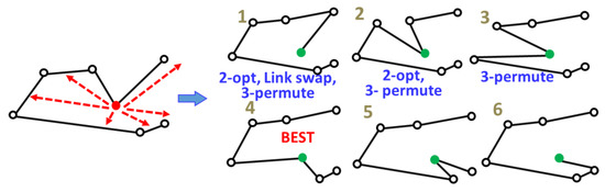
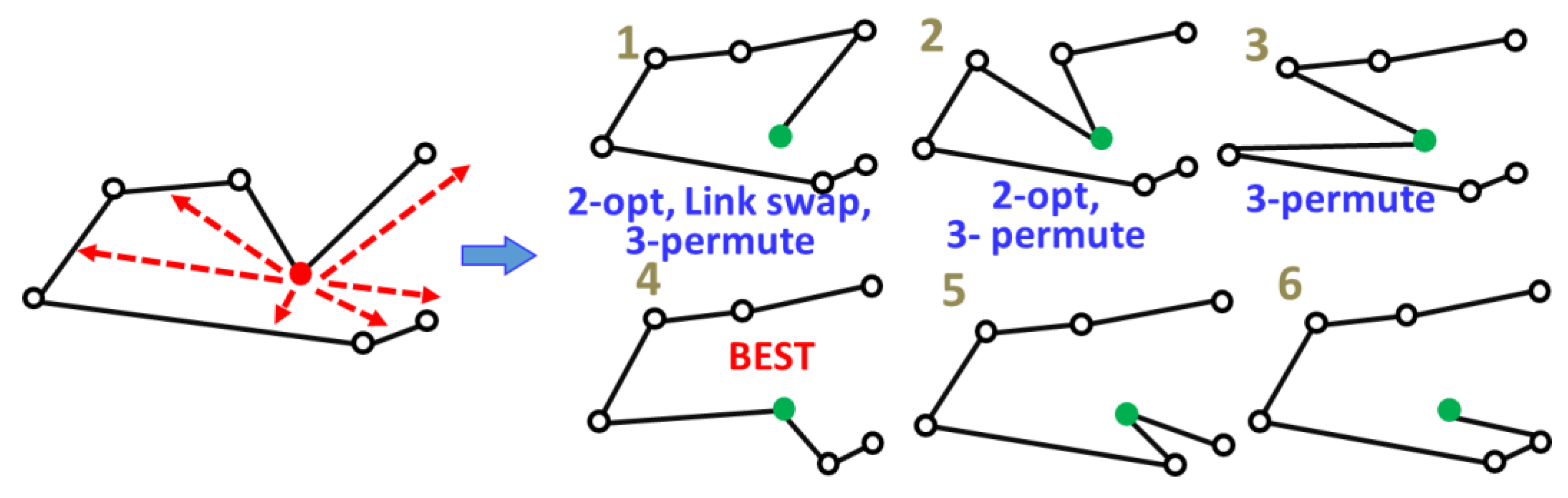
Relocate: The highlighted target in the start tour in Figure 8 can swap to six different positions. By analyzing these six results, we can observe that the tours 1 to 3 are also possible outcomes of 3–permute. Tours 1 and 2 are also possible outcomes of 2-opt and tour 1 can be an outcome of link swap. However, the rest of the tours are unique, and only possible to produce by the relocate operator. Only the relocate operator can produce the best result in this example (tour 4).

Figure 8. Six neighboring solutions created by relocate, of which three are unique.

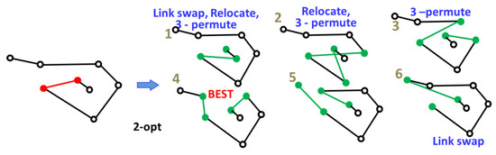
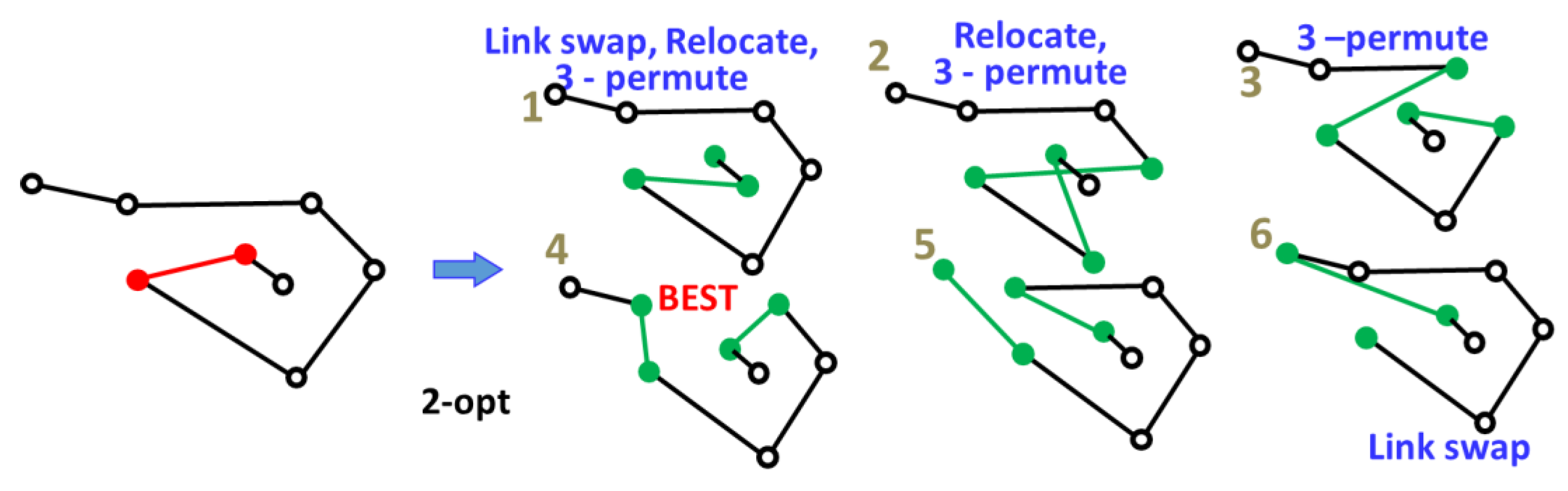
2-opt: In this method, two links are removed and two new ones are created. An example is shown in Figure 9, where the first removed link is fixed as the red one, which is highlighted, and the second one is varied. The resulting six new tours are shown. The other operators can generate four of them as well; however, two of them are unique. The best outcome is uniquely generated by the 2-opt operator.

Figure 9. Six neighboring solutions created by 2-opt, of which two are unique.

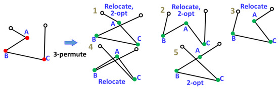
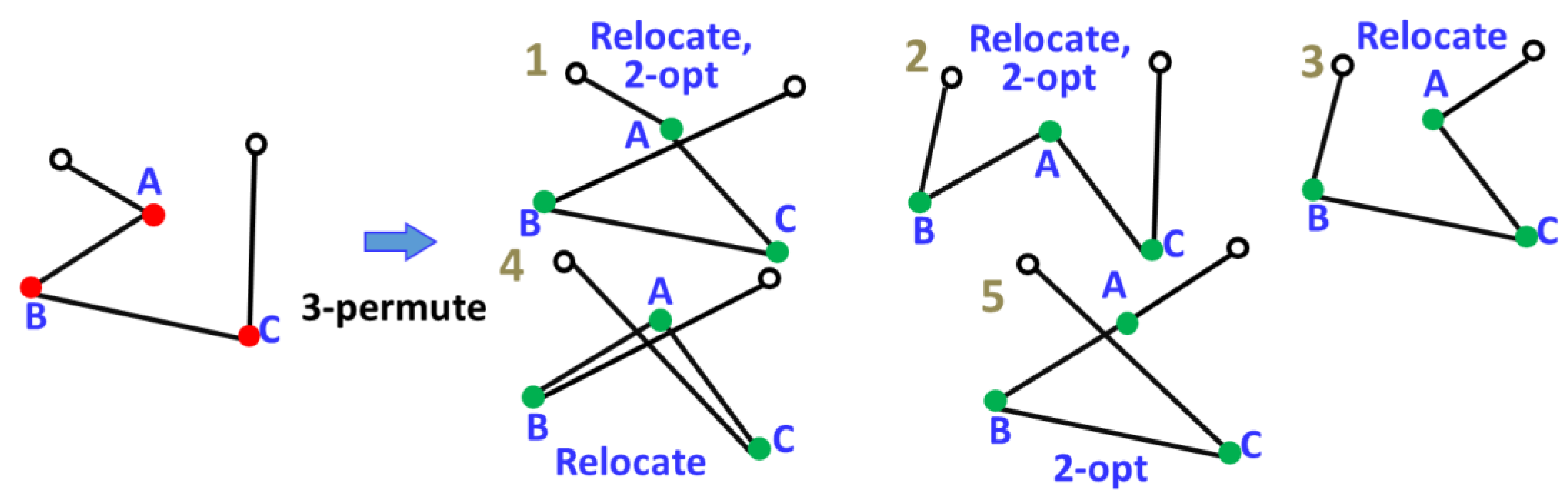
3-permute: The example in Figure 10 reveals that the operator does not produce even a single unique result. Therefore, if both relocate and 2-opt are used, this operator is redundant. Relocate can find four out of the five solutions, and 2-opt can find three.

Figure 10. Six neighboring solutions created by 3–permute, but none of them is unique.

A potential benefit of the 3–permute operator is that it needs to explore only a smaller neighborhood, O(N), in comparison to O(N²) of relocate and 2-opt. However, this smaller neighborhood is not extensive enough, as it misses the solutions shown in Figure 8 and Figure 9. Our experiments also show that the local search using 3-permute is consistently outperformed by the other operators. We, therefore, do not consider this operator further.

Link swap: This operator creates three alternatives for a selected link. Two of these are redundant with 2-opt, but the one which connects the two previous terminal points is unique (Figure 11). It is also the best one. Link swap is therefore worthwhile in cases when the terminal points are close to each other.

Figure 11. Three neighboring solutions created by link swap, of which the one connecting the terminal nodes is unique.

3. Performance of a Single Operator

We next test the performance of the different operators within a local search. For this, we need an initial tour to start with and a search strategy. These will be discussed first, followed by the experimental results.

3.1. Initial Solution

If the operator and search strategy are good, the choice of initialization should not matter much for the final result. We, therefore, consider only two choices:

• Random
• Heuristic (greedy)

Random initialization selects the nodes one by one randomly to create the initial tour.

A straightforward method for better initialization is greedy heuristic. It selects a random node as a starting point and always takes the closest unvisited node as the next target. Because of solving open-loop TSP, the starting point also matters in this case. We therefore systematically try all nodes as the starting point and generate N candidate tours using the greedy heuristics. Among N candidate tours, we select the shortest tour as the initial solution. Algorithm 1 presents the pseudocode for this.

Algorithm 1: Finding the heuristic initial path

HeuristicPath () InitialPath ← infinity FOR node ← 1 TO N DO  NewPath ← GreedyPath ( node )  IF Length ( NewPath ) < Length ( InitialPath ) THEN   InitialPath ← NewPath RETURN InitialPath

GreedyPath ( startNode ) NewPath [1] ← startNode FOR i ← 2 TO N DO  NewPath [i]  ← Nearest node from startNode  startNode    ← NewPath [i] RETURN NewPath

3.2. Search Strategy

For the search strategy we consider the following three choices:

• Best improvement
• First improvement
• Random search

Best improvement studies the entire neighborhood and selects the best one among all solutions. This can be impractical, especially if the neighborhood is large. The first improvement studies the neighborhood only until it founds any solution that provides improvement. It can be more practical as it moves on with the search quicker. Random search studies the neighbors in random order, and similar to the first improvements, accepts any new solution that improves.

We also consider repeated (multi-start) local search, which simply re-starts the search from scratch several times. This helps if the search is susceptible to getting stuck into a local minimum [39]. Moreover, every repeat is essentially a random attempt to converge to a local optimum; parallelization can be applied by running different repeats on different execution threads. O'Neil & Burtscher [40] and Al-Adwan et al. [41] preferred repeated local search, for TSP and Xiang et al. [42] for matrix multiplication to overcome local optima.

A pseudocode that covers all the search variants with all the operators is given in Algorithm 2. The only parameter is the number of iterations for which the search continues. First and best improvement searches can also be terminated when the entire neighborhood is searched without further improvement. This corresponds to the hill-climbing strategy.

Algorithm 2: Finding the improved tour by all the operators for different search strategies

LocalSearch ( InitialPath, OperationType ) Path ← InitialPath SWITCH SearchType  CASE RANDOM   FOR i ← 1 TO Iterations DO    NewPath ← NewRandomSolution ( Path, OperationType )    IF Length ( NewPath ) < Length ( Path ) THEN     Path ← NewPath  CASE FIRST   Path ← NewFirstSolution ( Path )  CASE BEST    Path ← NewBestSolution ( Path ) RETURN Path NewRandomSolution ( Path, OperationType ) SWITCH OperationType  CASE RELOCATE   Target ← Random ( 1, N )   Destination ← Random ( 1, N )   NewPath ← relocate ( Path, Target, Destination ) CASE 2OPT   FirstLink ← Random ( 1, N )   SecondLink ← Random ( 1, N )   NewPath ← 2Opt ( Path, FirstLink, SecondLink )  CASE LINKSWAP   Link ← Random ( 1, N )   NewPath ← linkSwap ( Path, Link ) RETURN NewPath NewFirstSolution ( Path, OperationType ) FOR i ← 1 TO N DO  FOR j ← 1 TO N DO    SWITCH OperationType    CASE RELOCATE     NewPath ← relocate ( Path, i, j )    CASE 2OPT     NewPath ← 2Opt ( Path, i, j )   IF Length ( NewPath ) < Length ( Path ) THEN    Path ← NewPath    RETURN Path  IF OperationType = LINKSWAP    NewPath ← linkSwap ( Path, i )   IF Length ( NewPath ) < Length ( Path ) THEN    Path ← NewPath    RETURN Path   NewBestSolution ( Path, OperationType ) FOR i ← 1 TO N DO  FOR j ← 1 TO N DO   SWITCH OperationType    CASE RELOCATE     NewPath ← relocate ( Path, i, j )    CASE 2OPT     NewPath ← 2Opt ( Path, i, j )   IF Length ( NewPath ) < Length ( Path ) THEN    Path ← NewPath  IF OperationType = LINKSWAP   NewPath ← linkSwap ( Path, i )   IF Length ( NewPath ) < Length ( Path ) THEN    Path ← NewPath RETURN Path

3.3. Results With A Single Operator

We first study how close the operators can improve paths to the optimum solutions using O–Mopsi and Dots datasets. Optimum paths were computed by branch-and-bound. Two results are reported:

• Gap (%)
• Instances solved (%)

The gap is the length of the optimum path divided by the length of the tour found by the local search (0% indicates optimum). The second result is the number of instances for which an optimum solution is found by the local search. We also express it in a percentage value, which indicates 100% means that the method finds the optimum solutions for all instances. We execute every operator individually with all search strategies on all O-Mopsi game instances. Repeated search is applied only for the random search with random initialization.

We combine the results of O-Mopsi and Dots datasets and report those in Table 2. In the table, we first write the gap values, and the percentage values of solved instances are written inside the parentheses. The 2-opt is the best individual operator. It reaches a 2% gap and solves 57% of all instances when starts from a random initialization, and 0.8% (73% instances) using the heuristic initialization. The repeats are important. With 25 repeats, the 2-opt solves 97% of all instances, and the mean gap is almost 0%.

Table 2. Combined results of single and subsequent application of random improvement with different operators averaged over O–Mopsi and Dots instances. The percentage of solved instances are shown inside the parenthesis. The number of iterations was fixed to 10000 for randomized search, whereas first and best improvements were iterated until convergence.

		Single Operator			Double Operators			Mix of Three
Initialization		Random	Heuristic	Repeated (25 times)	Repeated (25 times) Second Operator:			Repeated (25 times)
					Relocate	2-opt	Link swap	Subseq-uent	Mixed
	First	7% (30%)	1.0% (70%)	-	-	-	-	-	-
Reloc-ate	Best	6% (34%)	0.9% (72%)	-	-	-	-	-	-
	Random	6% (34%)	0.9% (71%)	0.18% (90%)	-	0.007% (98%)	0.032% (97%)	0.010% (98%)	0.005%(99.7%)
2-opt	First	2% (54%)	1.0% (70%)	-	-	-	-	-	-
	Best	2% (57%)	0.8% (73%)	-	-	-	-	-	-
	Random	2% (52%)	0.8% (73%)	0.02% (97%)	0.009% (98%)	-	0.018% (97%)	0.005% (99%)	0.005% (99.7%)
Link swap	Best	44% (5%)	2.9 (59%)	-	-	-	-	-	-
	Random	11% (31%)	3.0 (58%)	1.00% (77%)	0.019% (98%)	0.010% (97%)	-	0.006% (99%)	0.005% (99.7%)

The better initialization provides significant improvement in all cases, which indicates the search gets stuck into a local minimum. The choice of the search strategy, however, has only minor influence. We, therefore, consider only the random search in further experiments.

3.4. Combining the Operators

Our primary goal was to find an optimum solution for all game instances. The best combination (2-opt with a random search using 25 repeats) missed it for only 3% of instances. Nevertheless, these are relatively easy instances; therefore, they should all be solvable by the local search. We, therefore, consider combining different operators. We do this by applying a single run of the local search with one operator, and then continue the search with another operator. We consider all pairs and the subsequent combinations of all three operators.

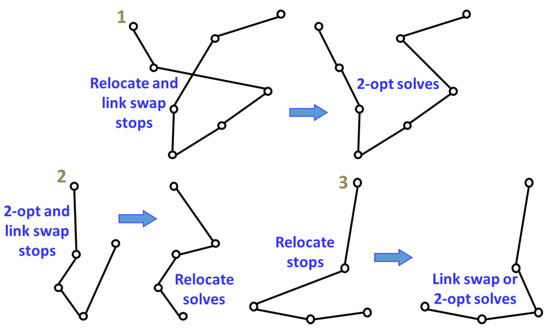
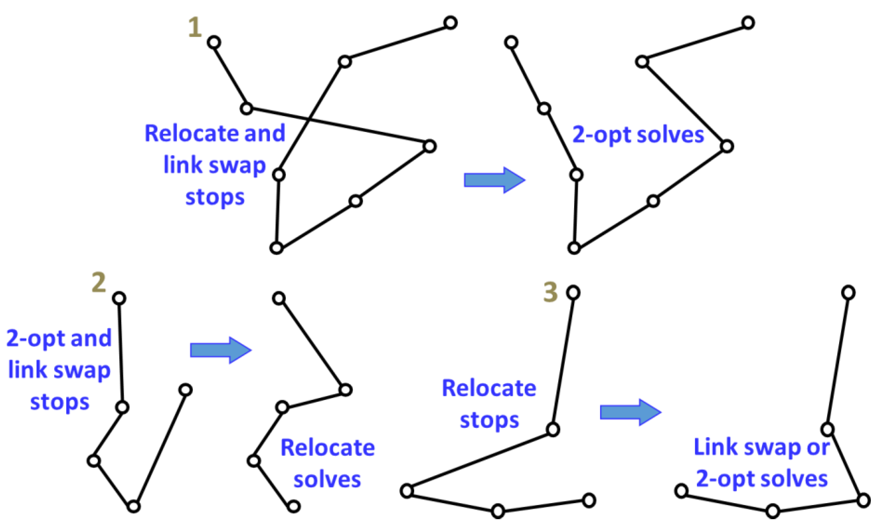
We tested all combinations but report only the results of 25 repeats using the random improvement (random initialization). From the results in Table 2, we can see that all combinations manage to solve a minimum of 97% of all instances and have a gap of 0.032% or less. The mixed variant with the order (2-opt + relocate + link swap) found the optimum solution for 99% cases. In this case, 2-opt solves already a 97% of all instances, then the consecutive relocate makes it 98%, and finally link swap makes it 99%. This shows that the operators have complementary search spaces; when one operator stops progressing, another one can still improve further. Examples are shown in Figure 12.

Figure 12. Operators have complementary search spaces.

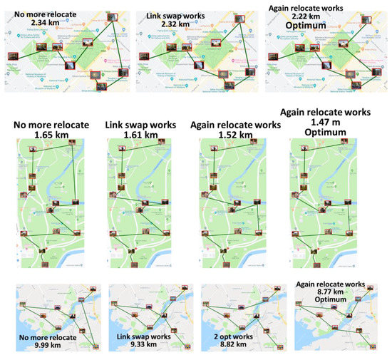
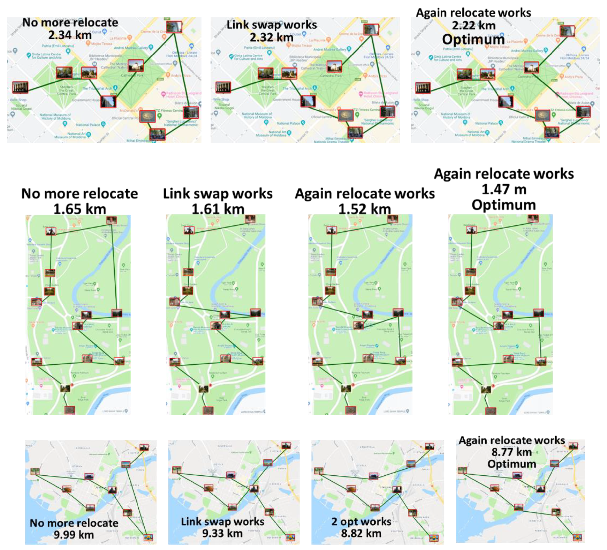
After being stopped, it is also possible that a single operator can start to work again when other operators make some improvement in the meantime. Hence, these works of other operators make the first operator alive again. Figure 13 has three such examples, where the first operator entraps into a local optimum. Then, other operators recover the process from the local optimum and improvement continues. Again, the first operator starts working later.

Figure 13. A single operator can re-work after being stuck with the help of other operators’ improvement.

In addition, we consider also mixing the operators randomly as follows. We perform only a single run of the local search for 10,000 iterations. However, instead of fixing the operator beforehand, we choose it randomly at every iteration. The pseudocode of the mixed variant is demonstrated in Algorithm 3. This random mixing solves all instances with having a 0% gap if we repeat the process for 25 times.

Algorithm 3: Finding a solution by mixing local search operators

RandomMixing ( NumberOfIteration, Path ) FOR i ← 1 TO NumberOfIteration DO  operation ← Random ( NodeSwap, 2opt, LinkSwap )  NewPath ← NewRandomSolution ( Path, operation )  IF Length ( NewPath ) < Length ( Path ) THEN    Path ← NewPath RETURN Path

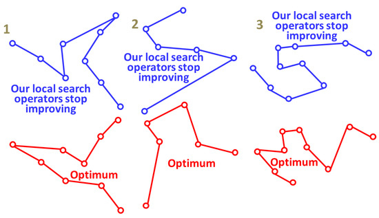
Lawler et al. [43] stated that local search algorithms get trapped in sub-optimal points. Here, we find that the operators, even when mixed, could not solve all the instances from any random initial solution. Figure 14 shows three examples where the search was stuck to a local optimum from where none of the operators can process further. In these cases, the repeated random mixed local search was needed to solve these instances.

Figure 14. Examples of local optima. Repeats overcome these.

4. Analysis of Repeated Random Mixed Local Search

We next analyze the performance of the repeated local search in more detail. We use both the 145 O–Mopsi instances and the larger Dots dataset, which contains 4226 computer-generated TSP instances. Here problem size varies from 4 to 31.

4.1. Effect of the repetitions

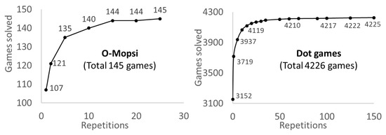
Figure 15 reports how many of the instances are solved when we increase the number of repeats. In the case of O–Mopsi, most instances (144) are solved already with 15 repeats, and all with 25 repeats. The results with the Dots instances are similar: 15–25 iterations are reasonably good, after which only 100 instances were not solved optimally. After 150 repeats, only one instance remains unsolved.

Figure 15. Instances solved as a function of the number of repetitions.

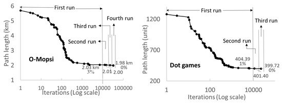
Figure 16 demonstrates the effect of repetition for a single (typical) instance as the average path length. We portray all improving steps from a random start in the first run. There is a similar kind of improving steps from different random starts in the consecutive runs. However, we only show more improved steps than the previous run. Thus, we can see there are very few better steps in higher runs, and three or four repeated runs are usually enough to achieve the optimum result. The gap values are also shown to demonstrate the closeness of our outcomes to the optimum result. In the first run, we usually achieve a result that is already very close to the optimum. The repetitions push the result to the global optimum, but they act merely as a fine tuner for the results. If we can settle the sub-optimal result very close to the global optimum, then a local search with only a few repeats would be sufficient for these datasets.

Figure 16. Typical example of the effect of repetition.

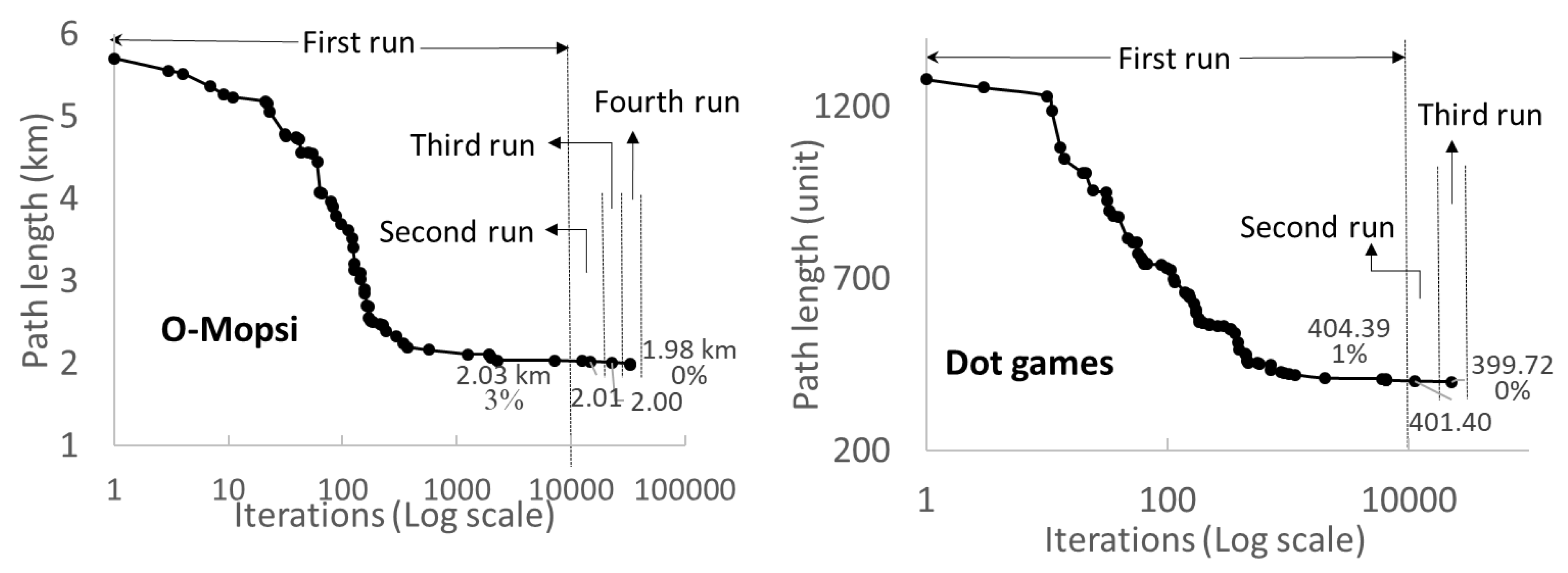
Next, we evaluate the total work based on the number of iterations and the number of repeats. We plot four different curves with random start repeated 1, 5, 15, and 25 times for the O–Mopsi instances. Figure 17 shows how close the path length becomes to the optimum during 10,000 iterations. A similar plot is also drawn for the Dots instances with 1, 5, 15, 25, 50, 100, and 150 repeats. All the curves coincide on each other so they appear as only one line in Figure 17.

Figure 17. Total amount of work.

4.2. Processing Time

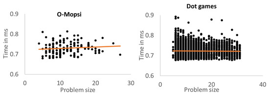
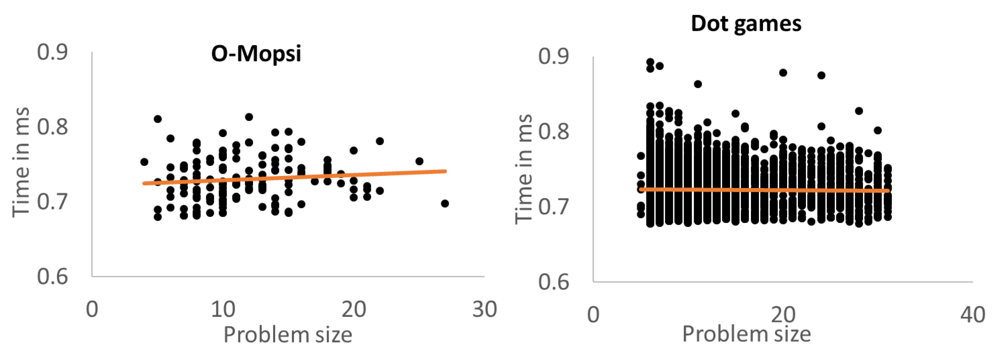
The time complexity of the method can be analyzed as follows. At each iteration, the algorithm tries to find improvement by a random local change. The effect of this change is tested in constant time. Only when improvement is found, the solution is updated accordingly, which takes O(N) time. Let us assume probability p for finding an improvement. The time complexity is, therefore, O(IR + pNIR), where I and R are the number of iterations and repetitions, respectively. The value for p is higher at the beginning, when the configuration is close to random and gradually decreases to zero when approaching to a saturation point (the solution that cannot be improved by any local operation). In our observations, p is small (0.002 on average for O–Mopsi and even lesser for Dots), so the time complexity reduces to O(IR), in practice. This means that the speed of the algorithm is almost independent on the problem size (see Figure 18).

Figure 18. Run time as a function of problem size.

In contrast, optimal solvers such as Concorde [17] have exponential time complexity. We are unable to find a complexity analysis for Concorde in literature, however, we estimate it empirically by analyzing the running time required by Concorde to solve TSPLIB [44] instances. From the website (http://www.math.uwaterloo.ca/tsp/concorde/benchmarks/bench99.html), we choose 105 instances with increasing problem sizes (N between 14 and 13509) and analyze the trend. According to this, Concorde has a complexity of (1.5e^(0.004N)). This implies that for small instances (up to several thousands) the algorithm is expected to be fast. However, the analysis also reveals that some points highly deviate from the expected line. This implies that some instances are more difficult to solve (with a higher number of nodes in the search tree) and require more time, such as the instance (d1291), with 1291 targets, which has almost 8 hours of running time where another instance (rl1304) with 1304 targets has only 22 minutes of running time. In comparison to that, Random Mix finishes more predictably.

Considering the repeats, we summarized the result in Table 3, which shows that a single run takes 0.8 ms and 25 repeats take 16 ms on an average, regardless of the dataset.

Table 3. Running time.

	Single Run	25 Repeats
O–Mopsi	0.8 ms	16 ms
Dots	0.7 ms	16 ms

4.3. Parameter Values

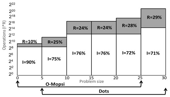
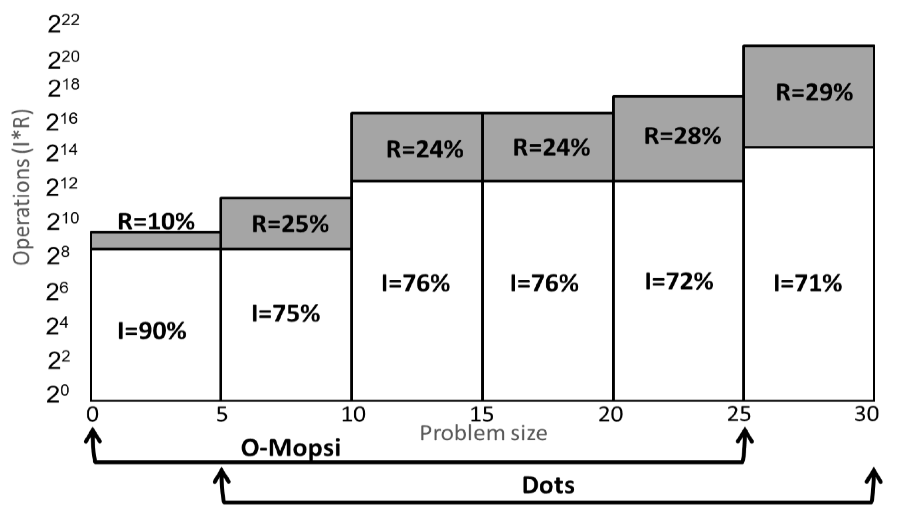
We investigate different values for the I and R parameters using grid-search and recorded how many operations are needed to solve different sized problems. The results are summarized in Figure 19. In this context, we want to mention, as there are not a sufficient number of samples with more than 25 targets in the O–Mopsi dataset and 30 targets in the Dots dataset, we ignore those samples. From the chart, we can conclude that proper parameter values to use for the O–Mopsi dataset are I = 2¹³ and R = 2⁵. The dots dataset requires higher values of I = 2¹⁵ and R = 2⁶. The relationship between I and R seems to stabilize for larger instances.

Figure 19. Required number of operations increases with problem size.

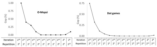
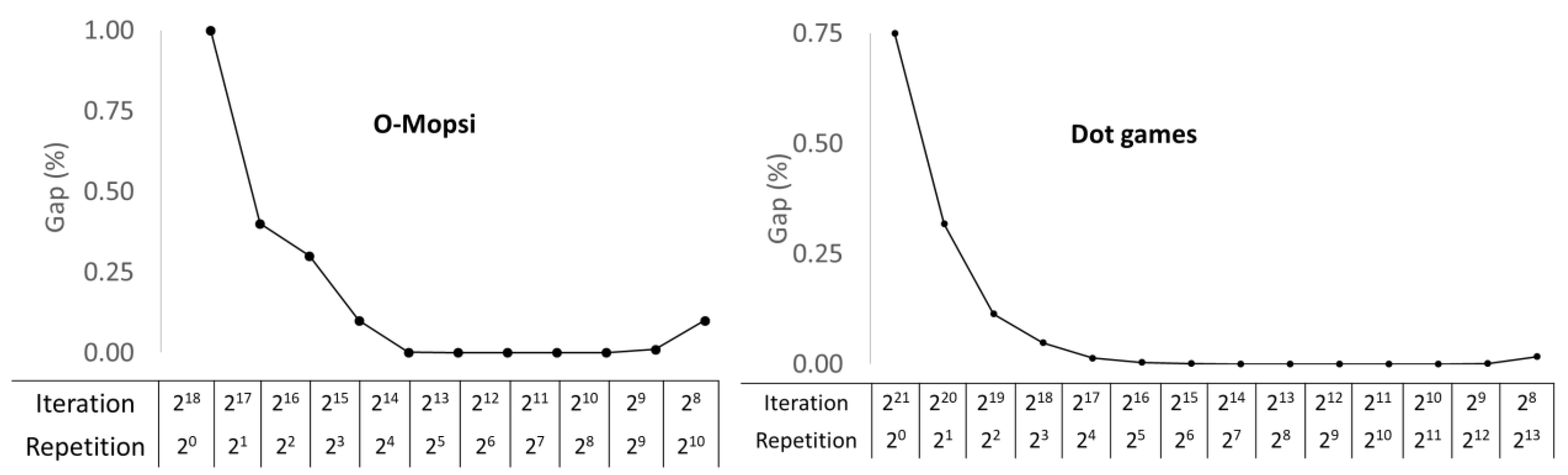
In Figure 20, we fix the product IR to 2¹⁸ (O–Mopsi) and 2²¹ (Dots) and vary their individual values. Typically, different same-product combinations are equally effective at solving the instances. However, using too few repetitions, the algorithm typically gets stuck at a local optimum, which is not the global one. On the other hand, when the number of iterations becomes too small, it is likely that some local operations can still improve the result (not saturated).

Figure 20. Gap variation with varied iterations and repetitions.

4.4. The Productivity of the Operators

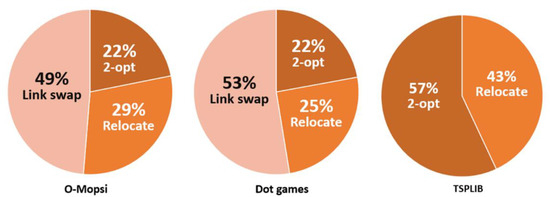
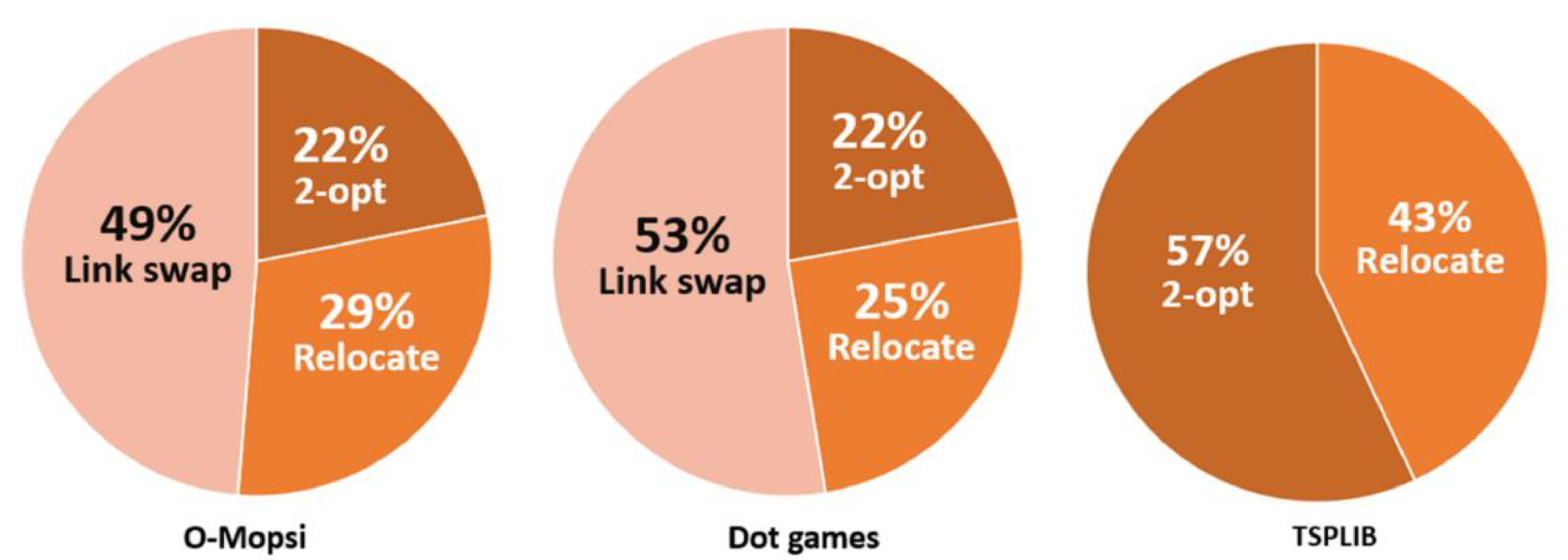
We next analyze the productivity of the operators, as follows. We count how many times each operator found an improvement in the solution. For this case, we also evaluate our operators by closed-loop instances (TSPLIB instances) [44]. We should mention here that closed-loop instances do not contain single links to swap. Therefore, the link swap operation is not possible for them. We can only use the relocate and 2-opt operators to solve TSPLIB problems. In this context, we want to mention that we choose 12 TSPLIB instances to test with problem size of 52–3795. These instances are significantly larger than O–Mopsi and Dots instances, and therefore, we used a much higher number of iterations (10⁸) and 25 repeats. The total distribution of the improvement achieved by operators is shown in Figure 21 both for the open-loop (O–Mopsi and Dot games) and closed-loop (TSPLIB) [44] cases. From the results, we can make the following observations.

Figure 21. Share of the improvements by all three operators both with the open-loop (O–Mopsi and Dot games) and closed-loop (TSPLIB) problem instances. With TSBPLIB, we use 10⁸ iterations and 25 repeats.

First, we can see that the 2-opt and relocate are almost equally productive in all cases. However, the situation changes dramatically from the closed-loop to the open-loop case. While 2-opt and relocate both have about a 50% share of all improvements in the closed-loop case (TSPLIB), they are inferior to the new link swap operator in case of open-loop test sets (O–Mopsi and Dots). The link swap operator dominates by a 50% share, while 2-opt and relocate have roughly a 25% share each. The relocate operator becomes also slightly more productive than 2-opt.

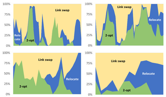
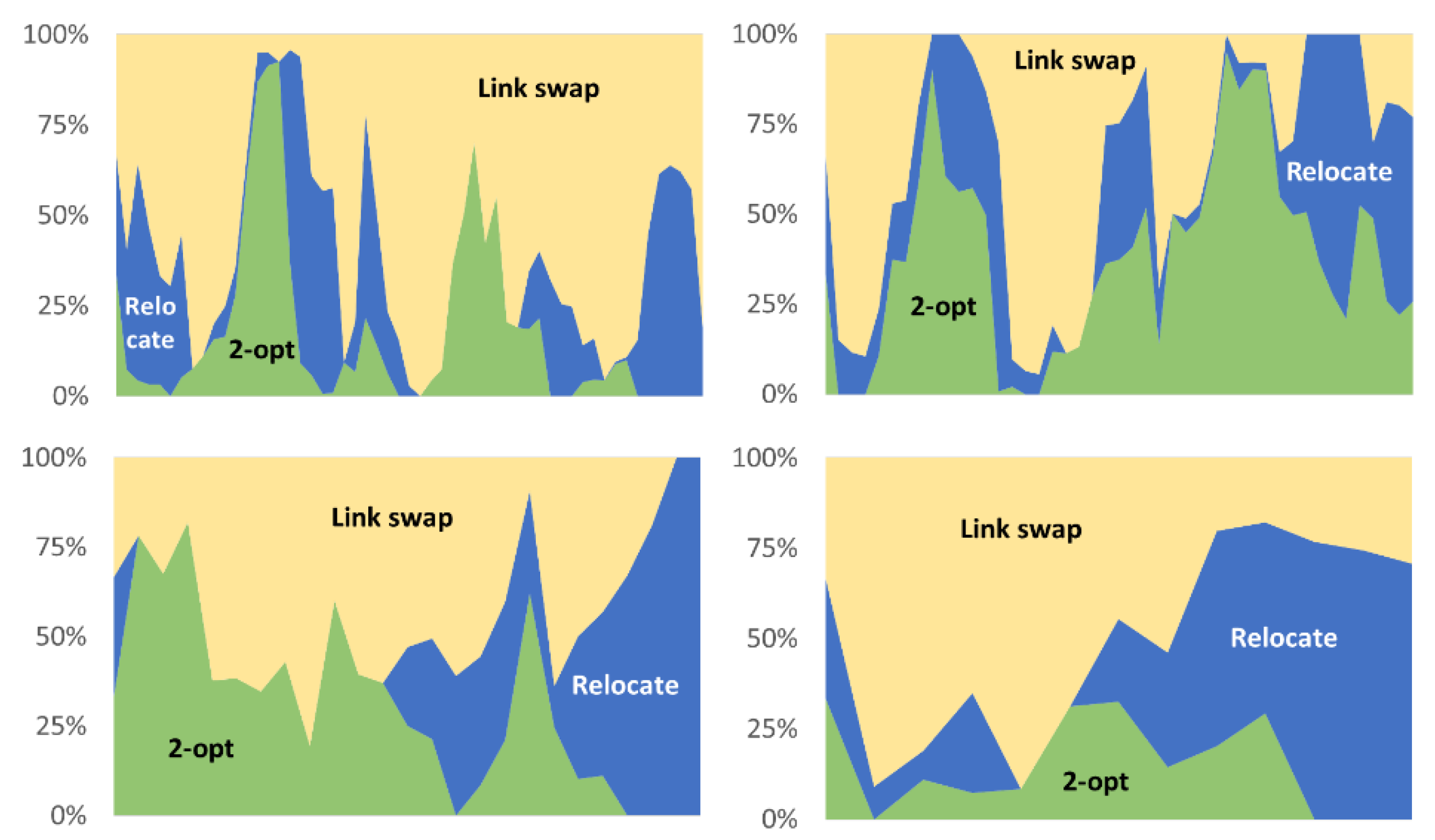
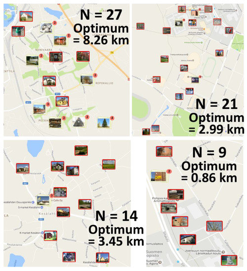
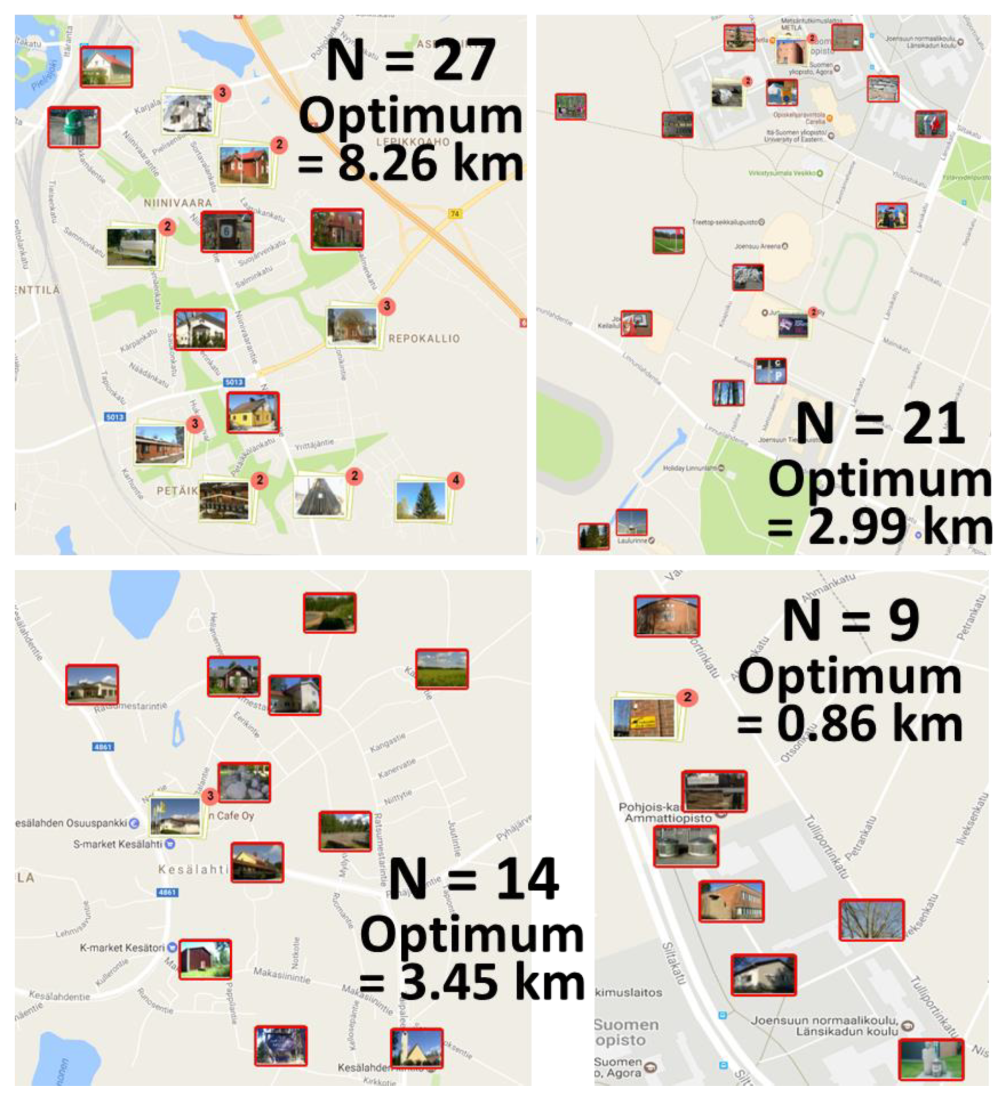
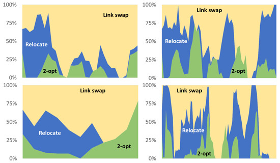
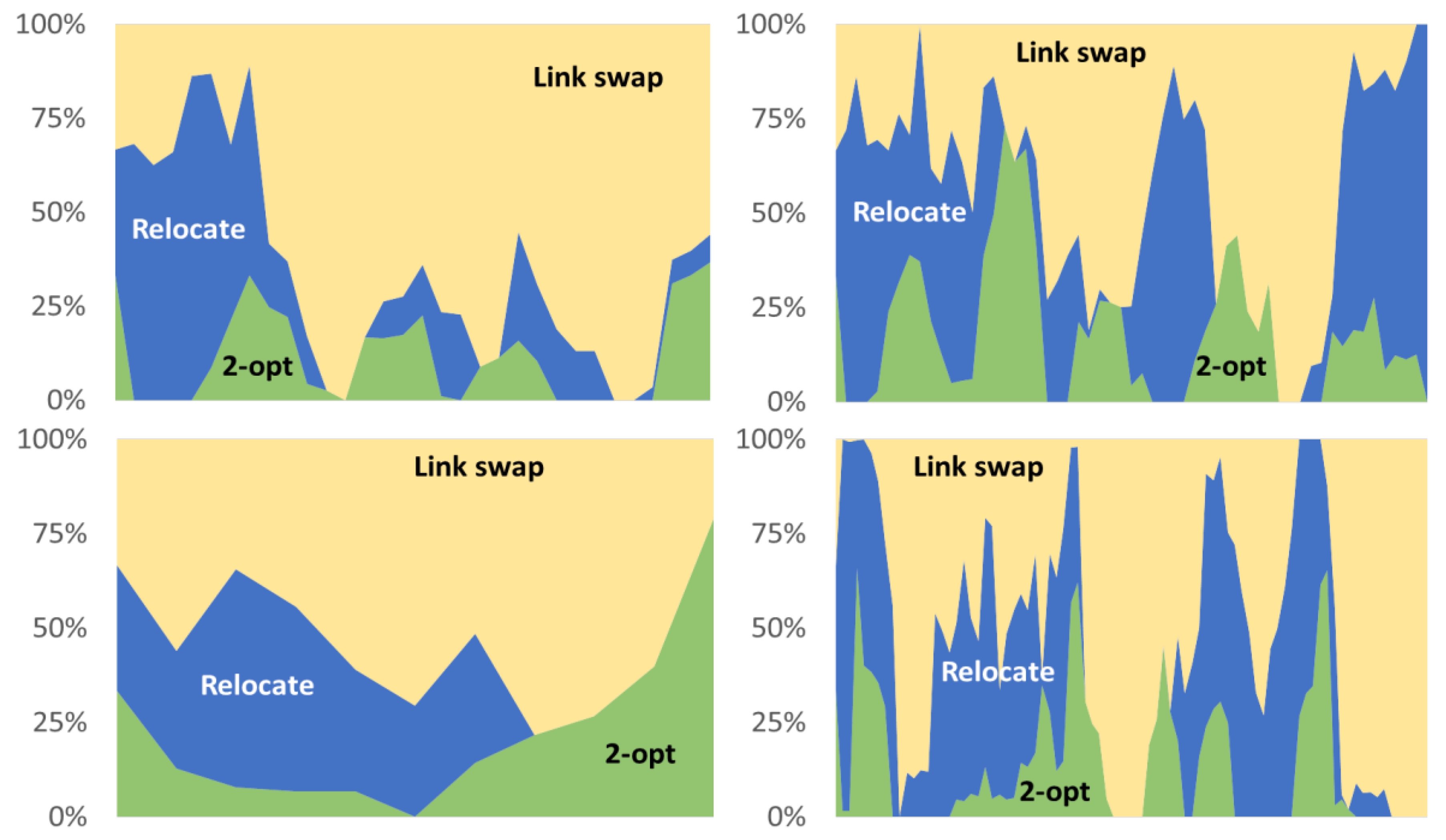
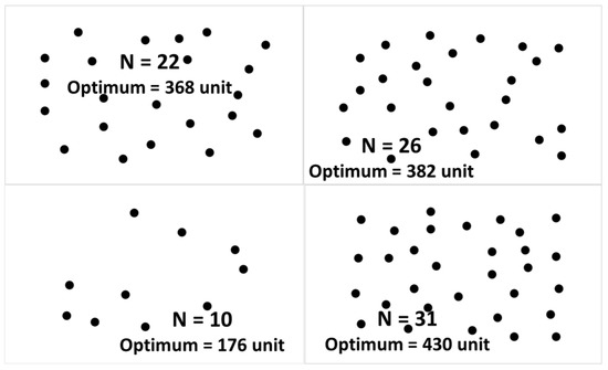
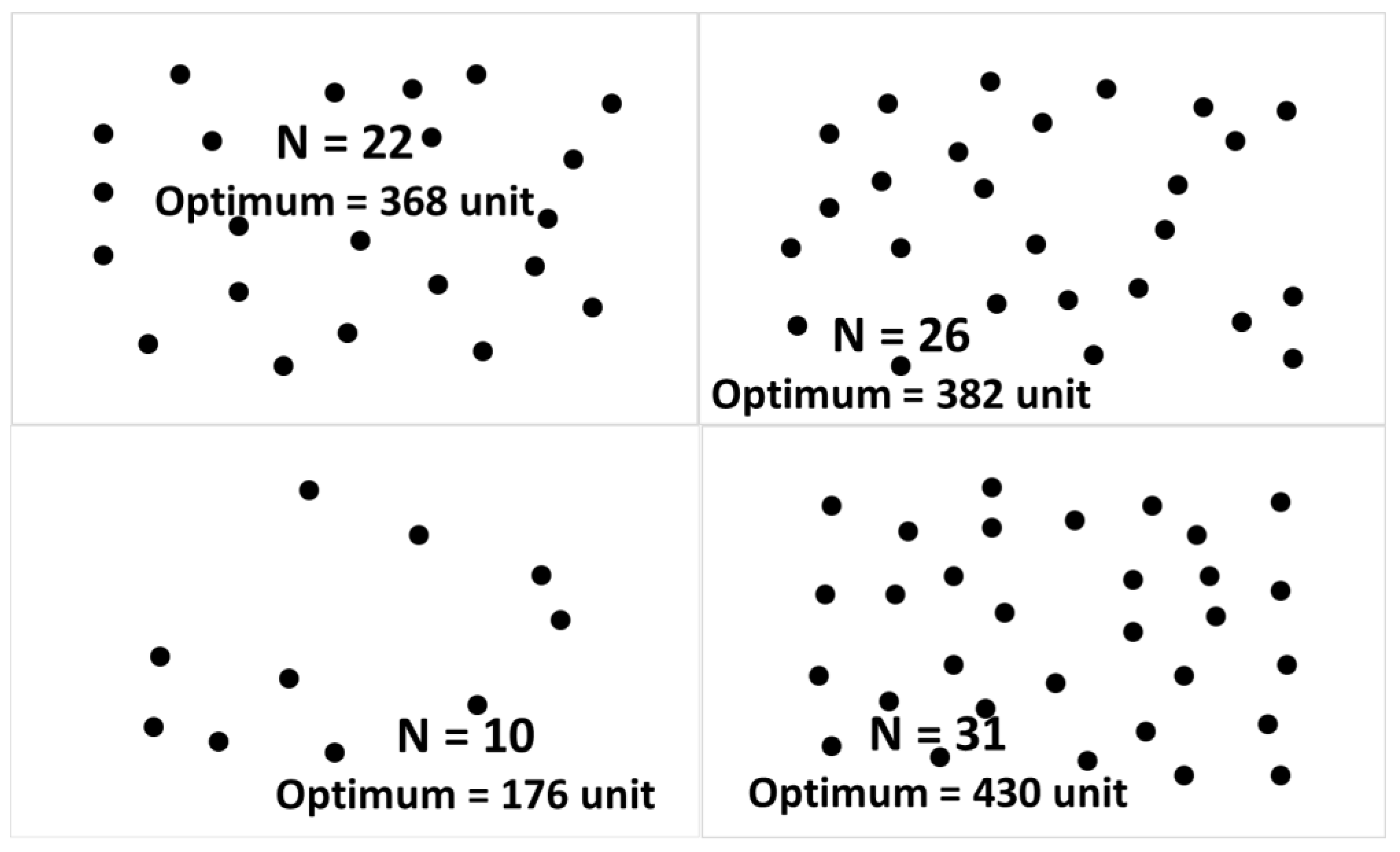
One question is whether all operators work equally efficiently at the beginning of the search, when there is more room for improvements, as they do at the end of the search when the improvements are harder to find. We select four typical O-Mopsi game examples and find the productivity of the operators through the total search spaces (Figure 22). We plot them in Figure 23. Similarly, Figure 24 shows the productivity of operators along the search spaces of four typical dot games. We plot those games in Figure 25. The diagrams show that there are no visible patterns to be observed. All operators remain productive at all stages of the search. Link swap is the most active and relocate is slightly more productive at the end of the search with the O–Mopsi instances.

Figure 22. Productivity of the operators during the search with for 4 different O–Mopsi instances.

Figure 23. Screenshots of the 4 different O–Mopsi instances (in the same order).

Figure 24. Productivity of the operators during the search with for 4 different Dots instances.

Figure 25. Screenshots of 4 different dots instances (in the same order).

5. Stochastic Variants

We consider repeat to overcome the local optimum values. However, there are several other methods to overcome local optimum values using tabu search [45], simple simulated annealing and combined variants [46,47,48,49,50], genetic algorithm [51,52,53,54]. Besides these, Quintero–Araujo et al. [55] combined iterated local search and Monte Carlo simulation on vehicle routing problems. We compared our results with some of these methods; additionally, we consider two stochastic variants of the local search:

• Tabu search [45]
• Simulated annealing [47]

Tabu search is a metaheuristic first introduced by Glover [45]. The idea is to allow uphill moves that worsen the solution to avoid being stuck in a local optimum. It forces the search to new directions. A tabu list of previously considered solutions, or moves, is maintained to prevent the search from going into cycles around the local optima.

We incorporate the tabu search with our local search as follows. When an improvement is found in the solution, we mark the added links as tabu. These links are not allowed to be changed in the next 0.2⋅N iterations. We use the best improvement as the search strategy. Table 4 shows results of tabu search for O-Mopsi and Dots games.

Table 4. Comparison of Tabu search and simulated annealing (SA) result with random mixed local search result with the same iteration and repetition for O–Mopsi and dot instances.

		Repeated (25 times)
		Gap (avg.)	Not Solved
O–Mopsi	Random mixed local search	0%	0
	Tabu search	0%	0
	Simulated annealing (SA)	0%	0
Dots	Random mixed local search	0.001%	1
	Tabu search	0.0003%	3
	SA	0.007%	10

Simulated annealing (SA) is another approach to make the search stochastic. Although there are a large number of adaptive simulated annealing variants, we consider a simpler one, the noising method of Charon and Hudry [47]. The idea is to add random noise to the cost function to allow uphill moves and therefore avoid local optima. The noise is a random number between r ∈ [0, ± r_max], and acts as a multiplier for the noisy cost function: f_noise = r⋅f. The noise starts from r_max = 1 and decreases at every iteration by a constant 2/T, where T is the number of iterations. The noise reaches r = 0 halfway, and the search then reduces back to normal local search by using normal cost function (f) for the remaining iterations. We apply a random mixed local search with 25 repeats. Table 4 also shows simulated annealing results for O-Mopsi and Dots instances.

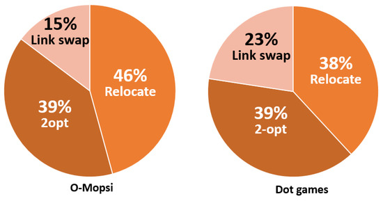
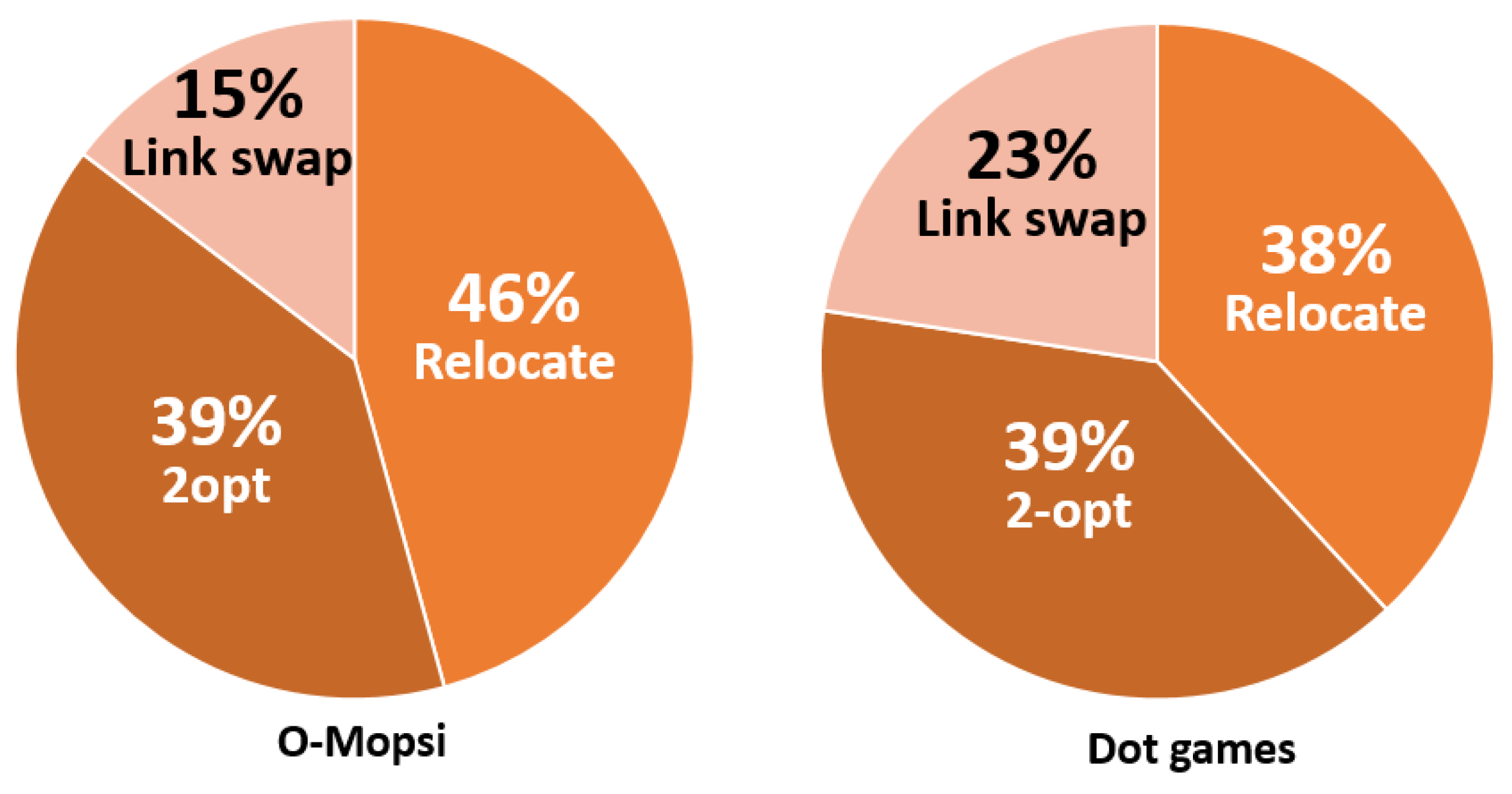
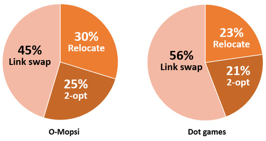
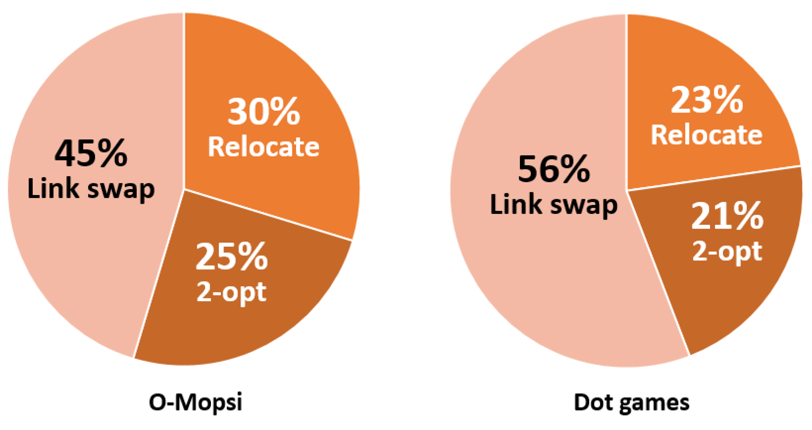
Finding the productivity of the operators as in Figure 21 for random mixed local search, we consider finding out the same in case of tabu search and simulated annealing. From a random mixed local search, we found that link swap was the most effective operation. Figure 26 illustrates that in tabu search, link swap is the least effective. However, link swap is again the most effective for the simulated annealing, as shown in Figure 27. We mark the added links as forbidden for tabu search, so link swap becomes too restrictive in this case. This makes link swap often non-working.

Figure 26. Share of improvement by all three methods for Tabu search.

Figure 27. Share of improvement by all three methods for simulated annealing (SA).

We compare the performance of random mixed local search, tabu search, and simulated annealing for O-Mopsi and dots games in Table 5. We study the gap value and execution time for every method. Results show that neither tabu nor simulated annealing improved the performance of the random mixed local search algorithm.

Table 5. Summary of overall results (mean).

Results	Random mix		Tabu		SA
	Gap	Time	Gap	Time	Gap	Time
O–Mopsi	0%	<1 s	0%	1.3 s	0 %	<1 s
Dots	0.001%	<1 s	0.0003%	1.3 s	0.007%	<1 s

6. Discussion

We have studied the open-loop variant of TSP to find out which operators work best. Two new operators were proposed: link swap and 3–permute. The link swap operator was shown to be the most productive. Even though 2-opt works best as a single operator, the best results are obtained using a mixture of all three operators (2-opt, relocate, link swap). The new operator, link swap, provides, 50% of all the improvements, while 2-opt and relocate have roughly a 25% share each. To sum up, the link swap operator is the most efficient operator in the mix.

For our problem instances up to size 31, the proposed combination of the local search (random mixed local search) finds the optimum solution in all O–Mopsi instances, and in all except one, Dots problem instances. Iterations and repetitions are the most significant parameters of the proposed method. Additionally, a suitable number of iterations and repetitions are essential with respect to the problem size, which is 2¹³ and 2⁵ for the O–Mopsi dataset, and 2¹⁵ and 2⁶ for the Dots dataset. For O–Mopsi instances, processing times are 0.8 ms (single) and 16 ms (repeats). For Dots instances, processing times are 0.7 ms (single) and 16 ms (repeats). The overall complexity of the algorithm mainly depends on the number of iterations and repeats. Furthermore, considering the multi-threaded platform, different repeats can work simultaneously to decrease the processing time by a factor of a number of threads.

Tabu search and simulated annealing were also considered but they did not provide further improvements in our tests. The productivity of the operators was consistent with those of the local search. We conclude that the local search is sufficient for our application where the optimum result is needed in real-time, and the occasional sub-optimal result can be tolerated.

The limitation of the new operator, link swap, is that it is suitable only for the open-loop case and does not apply to TSPLIB instances. Therefore, only 2-opt and relocate can be used for these instances. Without link swap, relocate also becomes weaker in the mixing algorithm, which might weaken the result.

References

- Garey, M.R.; Johnson, D.S. Computers and Intractability: A Guide to the Theory of Np-Completeness; W.H. Freeman & Co.: New York, NY, USA, 1979; ISBN 0716710455. [Google Scholar]
- Papadimitriou, C.H. The Euclidean travelling salesman problem is NP-complete. Theor. Comput. Sci. 1977, 4, 237–244. [Google Scholar] [CrossRef] [Scilit]
- Fränti, P.; Mariescu-Istodor, R.; Sengupta, L. O-Mopsi: Mobile Orienteering Game for Sightseeing, Exercising, and Education. ACM Trans. Multimed. Comput. Commun. Appl. 2017, 13, 56. [Google Scholar] [CrossRef] [Scilit]
- Vansteenwegen, P.; Souffriau, W.; Van Oudheusden, D. The orienteering problem: A survey. Eur. J. Oper. Res. 2011, 209, 1–10. [Google Scholar] [CrossRef] [Scilit]
- Chieng, H.H.; Wahid, N. A Performance Comparison of Genetic Algorithm’s Mutation Operators in n-Cities Open Loop Travelling Salesman Problem. In Recent Advances on Soft Computing and Data Mining. Advances in Intelligent Systems and Computing; Herawan, T., Ghazali, R., Deris, M., Eds.; Springer: Berlin/Heidelberg, Germany, 2014; Volume 287. [Google Scholar]
- Gavalas, D.; Konstantopoulos, C.; Mastakas, K.; Pantziou, G. A survey on algorithmic approaches for solving tourist trip design problems. J. Heuristics 2014, 20, 291–328. [Google Scholar] [CrossRef] [Scilit]
- Golden, B.L.; Levy, L.; Vohra, R. The Orienteering Problem. Nav. Res. Logist. 1987, 34, 307–318. [Google Scholar] [CrossRef] [Scilit]
- Perez, D.; Togelius, J.; Samothrakis, S.; Rohlfshagen, P.; Lucas, S.M. Automated Map Generation for the Physical Traveling Salesman Problem. IEEE Trans. Evol. Comput. 2014, 18, 708–720. [Google Scholar] [CrossRef] [Scilit]
- Sengupta, L.; Mariescu-Istodor, R.; Fränti, P. Planning your route: Where to start? Comput. Brain Behav. 2018, 1, 252–265. [Google Scholar] [CrossRef] [Scilit]
- Sengupta, L.; Fränti, P. Predicting difficulty of TSP instances using MST. In Proceedings of the IEEE International Conference on Industrial Informatics (INDIN), Helsinki, Finland, June 2019; pp. 848–852. [Google Scholar]
- Dantzig, G.B.; Fulkerson, D.R.; Johnson, S.M. Solution of a Large Scale Traveling Salesman Problem; Technical Report P-510; RAND Corporation: Santa Monica, CA, USA, 1954. [Google Scholar]
- Held, M.; Karp, R.M. The traveling salesman problem and minimum spanning trees: Part II. Math. Program. 1971, 1, 6–25. [Google Scholar] [CrossRef] [Scilit]
- Padberg, M.; Rinaldi, G. A branch-and-cut algorithm for the resolution of large-scale symmetric traveling salesman problems. SIAM Rev. 1991, 33, 60–100. [Google Scholar] [CrossRef] [Scilit]
- Grötschel, M.; Holland, O. Solution of large-scale symmetric travelling salesman problems. Math. Program. 1991, 51, 141–202. [Google Scholar] [CrossRef] [Scilit]
- Applegate, D.; Bixby, R.; Chvatal, V. On the solution of traveling salesman problems. Documenta Mathematica Journal der Deutschen Mathematiker-Vereinigung. Int. Congr. Math. 1988, Extra Volume III, 645–656. [Google Scholar]
- Laporte, G. The traveling salesman problem: An overview of exact and approximate algorithms. Eur. J. Oper. Res. 1992, 59, 231–247. [Google Scholar] [CrossRef] [Scilit]
- Applegate, D.L.; Bixby, R.E.; Chvatal, V.; Cook, W.J. The Traveling Salesman Problem: A Computational Study; Princeton University Press: Princeton, NJ, USA, 2011. [Google Scholar]
- Johnson, D.S.; Papadimitriou, C.H.; Yannakakis, M. How easy is local search? J. Comput. Syst. Sci. 1988, 37, 79–100. [Google Scholar] [CrossRef] [Scilit]
- Clarke, G.; Wright, J.W. Scheduling of Vehicles from a Central Depot to a Number of Delivery Points. Oper. Res. 1964, 12, 568–581. [Google Scholar] [CrossRef] [Scilit]
- Christofides, N. Worst-Case Analysis of a New Heuristic for the Travelling Salesman Problem (Technical Report388); Graduate School of Industrial Administration, Carnegie Mellon University: Pittsburgh, PA, USA, 1976. [Google Scholar]
- Johnson, D.S.; McGeoch, L.A. The traveling salesman problem: A case study in local optimization. Local Search Comb. Optim. 1997, 1, 215–310. [Google Scholar]
- Croes, G.A. A Method for Solving Traveling-Salesman Problems. Oper. Res. 1958, 6, 791–812. [Google Scholar] [CrossRef] [Scilit]
- Lin, S.; Kernighan, B.W. An effective heuristic algorithm for the traveling-salesman problem. Oper. Res. 1973, 21, 498–516. [Google Scholar] [CrossRef] [Scilit]
- Rego, C.; Glover, F. Local search and metaheuristics. In The Traveling Salesman Problem and Its Variations; Springer: Boston, MA, USA, 2007; pp. 309–368. [Google Scholar]
- Okano, H.; Misono, S.; Iwano, K. New TSP construction heuristics and their relationships to the 2-opt. J. Heuristics 1999, 5, 71–88. [Google Scholar] [CrossRef] [Scilit]
- Johnson, D.S.; McGeoch, L.A. Experimental analysis of heuristics for the STSP. In The Traveling Salesman Problem and Its Variations; Springer: Boston, MA, USA, 2007; pp. 369–443. [Google Scholar]
- Aarts, E.; Aarts, E.H.; Lenstra, J.K. (Eds.) Local Search in Combinatorial Optimization; Princeton University Press: Princeton, NJ, USA, 2003. [Google Scholar]
- Jünger, M.; Reinelt, G.; Rinaldi, G. The traveling salesman problem. Handb. Oper. Res. Manag. Sci. 1995, 7, 225–330. [Google Scholar]
- Laporte, G. A concise guide to the traveling salesman problem. J. Oper. Res. Soc. 2010, 61, 35–40. [Google Scholar] [CrossRef] [Scilit]
- Ahuja, R.K.; Ergun Ö Orlin, J.B.; Punnen, A.P. A survey of very large-scale neighborhood search techniques. Discret. Appl. Math. 2002, 123, 75–102. [Google Scholar] [CrossRef] [Scilit]
- Rego, C.; Gamboa, D.; Glover, F.; Osterman, C. Traveling salesman problem heuristics: Leading methods, implementations and latest advances. Eur. J. Oper. Res. 2011, 211, 427–441. [Google Scholar] [CrossRef] [Scilit]
- Matai, R.; Singh, S.; Mittal, M.L. Traveling salesman problem: An overview of applications, formulations, and solution approaches. In Traveling Salesman Problem, Theory and Applications; IntechOpen: London, UK, 2010. [Google Scholar]
- Laporte, G. The vehicle routing problem: An overview of exact and approximate algorithms. Eur. J. Oper. Res. 1992, 59, 345–358. [Google Scholar] [CrossRef] [Scilit]
- Vidal TCrainic, T.G.; Gendreau, M.; Prins, C. Heuristics for multi-attribute vehicle routing problems: A survey and synthesis. Eur. J. Oper. Res. 2013, 231, 1–21. [Google Scholar] [CrossRef] [Scilit]
- Gendreau, M.; Hertz, A.; Laporte, G. New insertion and postoptimization procedures for the traveling salesman problem. Oper. Res. 1992, 40, 1086–1094. [Google Scholar] [CrossRef] [Scilit]
- Mersmann, O.; Bischl, B.; Bossek, J.; Trautmann, H.; Wagner, M.; Neumann, F. Local Search and the Traveling Salesman Problem: A Feature-Based Characterization of Problem Hardness. In Lecture Notes in Computer Science, Proceedings of the Learning and Intelligent Optimization, Paris, France, 16–20 January 2012; Springer: Berlin/Heidelberg, Germany, 2012; Volume 7219, p. 7219. [Google Scholar]
- Helsgaun, K. An effective implementation of the Lin–Kernighan traveling salesman heuristic. Eur. J. Oper. Res. 2000, 126, 106–130. [Google Scholar] [CrossRef] [Scilit]
- Pan, Y.; Xia, Y. Solving TSP by dismantling cross paths. In Proceedings of the IEEE International Conference on Orange Technologies, Xian, China, 20–23 September 2014; pp. 121–124. [Google Scholar]
- Martí, R. Multi-start methods. In Handbook of Metaheuristics; Springer: Berlin/Heidelberg, Germany, 2003; pp. 355–368. [Google Scholar]
- O’Neil, M.A.; Burtscher, M. Rethinking the parallelization of random-restart hill climbing: A case study in optimizing a 2-opt TSP solver for GPU execution. In Proceedings of the 8th Workshop on General Purpose Processing using GPUs, San Francisco, CA, USA, 7 February 2015; pp. 99–108. [Google Scholar]
- Al-Adwan, A.; Sharieh, A.; Mahafzah, B.A. Parallel heuristic local search algorithm on OTIS hyper hexa-cell and OTIS mesh of trees optoelectronic architectures. Appl. Intell. 2019, 49, 661–688. [Google Scholar] [CrossRef] [Scilit]
- Xiang, Y.; Zhou, Y.; Chen, Z. A local search based restart evolutionary algorithm for finding triple product property triples. Appl. Intell. 2018, 48, 2894–2911. [Google Scholar] [CrossRef] [Scilit]
- Lawler, E.L.; Lenstra, J.K.; Rinnooy Kan AH, G.; Shmoys, D.B. The Traveling Salesman Problem; A Guided Tour of Combinatorial Optimization; Publisher Wiley: Chichester, UK, 1985. [Google Scholar]
- Reinelt, G. A traveling salesman problem library. INFORMS J. Comput. 1991, 3, 376–384. [Google Scholar] [CrossRef] [Scilit]
- Glover, F. Tabu Search-Part I. ORSA J. Comput. 1989, 1, 190–206. [Google Scholar] [CrossRef] [Scilit]
- Kirkpatrick, S.; Gelatt, C.D.; Vecchi, M.P. Optimization by simulated annealing. Science 1983, 220, 671–680. [Google Scholar] [CrossRef] [Scilit] [PubMed]
- Charon, I.; Hurdy, O. Application of the noising method to the travelling salesman problem. Eur. J. Oper. Res. 2000, 125, 266–277. [Google Scholar] [CrossRef] [Scilit]
- Chen, S.M.; Chien, C.Y. Solving the traveling salesman problem based on the genetic simulated annealing ant colony system with particle swarm optimization techniques. Expert Syst. Appl. 2011, 38, 14439–14450. [Google Scholar] [CrossRef] [Scilit]
- Ezugwu, A.E.S.; Adewumi, A.O.; Frîncu, M.E. Simulated annealing based symbiotic organisms search optimization algorithm for traveling salesman problem. Expert Syst. Appl. 2017, 77, 189–210. [Google Scholar] [CrossRef] [Scilit]
- Geng, X.; Chen, Z.; Yang, W.; Shi, D.; Zhao, K. Solving the traveling salesman problem based on an adaptive simulated annealing algorithm with greedy search. Appl. Soft Comput. 2011, 11, 3680–3689. [Google Scholar] [CrossRef] [Scilit]
- Albayrak, M.; Allahverdi, N. Development a new mutation operator to solve the Traveling Salesman Problem by aid of Genetic Algorithms. Expert Syst. Appl. 2011, 38, 1313–1320. [Google Scholar] [CrossRef] [Scilit]
- Nagata, Y.; Soler, D. A new genetic algorithm for the asymmetric traveling salesman problem. Expert Syst. Appl. 2012, 39, 8947–8953. [Google Scholar] [CrossRef] [Scilit]
- Singh, S.; Lodhi, E.A. Study of variation in TSP using genetic algorithm and its operator comparison. Int. J. Soft Comput. Eng. 2013, 3, 264–267. [Google Scholar]
- Vashisht, V.; Choudhury, T. Open loop travelling salesman problem using genetic algorithm. Int. J. Innov. Res. Comput. Commun. Eng. 2013, 1, 112–116. [Google Scholar]
- Quintero-Araujo, C.L.; Gruler, A.; Juan, A.A.; Armas, J.; Ramalhinho, H. Using simheuristics to promote horizontal collaboration in stochastic city logistics. Prog. Artif. Intell. 2017, 6, 275. [Google Scholar] [CrossRef] [Scilit]
© 2019 by the authors. Licensee MDPI, Basel, Switzerland. This article is an open access article distributed under the terms and conditions of the Creative Commons Attribution (CC BY) license (http://creativecommons.org/licenses/by/4.0/).