Dependence of Dispersion on Metamaterial Structural Parameters and Dispersion Management

Featured Application

Although this is a theoretical work, it studies the dispersion characteristics in metamaterials in depth and discovers many results with potential applications in optical transmission.

Abstract

This paper compares the dispersion in metamaterials (MMs) and some Thorlabs’ conventional glass, and finds that MMs may exhibit much more substantial dispersion (e.g., three orders of magnitude larger dispersion). With such large dispersion, a transmission more than 22 km is impossible because of pulse splitting resulting from the third-order dispersion. However, MMs are artificial materials with their electric and magnetic plasma frequencies tunable depending upon their structures. We take advantage of such tunability to tailor the dispersive response of MMs and investigate the dependence of dispersion on the MM structural parameters. We make dispersion management by (1) searching for the existence of some ‘good’ dispersion points and numerically demonstrating 90 km long transmission with almost no pulse width expansion and any impact from a higher order dispersion in the MM we designed; and (2) searching for the possibility for group-velocity dispersion (GVD) compensation and demonstrating 120 km transmission by configuring the dispersion-engineered MM.

1. Introduction

Chromatic dispersion is the phenomenon in which the phase velocity of an optical wave depends on its frequency because of the material and structure’s geometry [1]. Metamaterials (MMs) are materials engineered to have designed properties beyond those available in nature, with applications in all aspects of materials science [2,3]. In particular, MMs have shown promise for next generation optical materials with electromagnetic responses that cannot be obtained from conventional media. MMs are made from assemblies of multiple elements fashioned from composite materials, such as metals, plastics, or dielectric media. The materials are usually arranged in repeating patterns, at scales that are smaller than the wavelengths of the phenomena they influence. The regularly stacked structures in MMs may entail stronger chromatic dispersion. This paper makes a quantitative comparison of MMs to some conventional Thorlabs’ glass [4,5], and discloses that MMs may have dispersion surpassing those of glass by three orders of magnitude. Since dispersion is a serious factor in MMs, dispersion management is an indispensable element while light propagates in MM waveguides, in which dispersive effects accumulate to set limits on both the distance and the bit rate of the data transfer.

Recent advances in nanofabrication and breakthroughs in the field of MMs [6,7,8,9,10,11,12] have opened up a new range of possibilities for obtaining optical properties on demand in MMs [13]. There is a research group now demonstrating that the group-velocity dispersion can be compensated by designing the phase-engineered MM, thus developing a new dispersion compensation technology [14]. The dispersive properties of most MMs are determined by the electric and magnetic plasma frequencies through the Drude model [15,16,17]. MMs are artificial materials with their electric and magnetic plasma frequencies tunable, depending upon their constituents and structures. Reconfigurable MMs provide flexibility for tuning them and result in tailored dispersive properties for dispersion management purposes. This paper studies the dependence of dispersion on the electric and magnetic plasma frequencies, and searches for the possibilities of dispersion management. Two approaches for the dispersion management are proposed. Demonstrations of a 90 km long transmission, with almost no pulse width expansion and any impact from a higher order dispersion in the MM we designed, and a 120 km transmission, by configuring the dispersion-engineered MMs, are numerically realized.

2. Theory of Light Pulse Propagations in MMs

Light is a type of electromagnetic wave and its propagation in MMs obeys Maxwell’s equations. The wave equation for the light pulse propagating in nonlinear dispersive MMs can then be deduced as follows:

$$\frac{{\partial }^{2}E}{\partial z^2}={\mu }_0{\epsilon }_0\frac{{\partial }^{2}E}{\partial t^2}+{\mu }_0\frac{{\partial }^2{P}_{NL}}{\partial t^2}.$$

(1)

It is assumed that $E=1/2A(z,t)\exp [i({\beta }_{0}z-\omega t)]+c.c$ and $P_{NL}={\epsilon }_0{\chi }^{(3)}{\left|E(z,t)\right|}^{2}E(z,t)$ with ${\chi }^{(3)}$ the third-order electric susceptibility. It is known that the relative dielectric constant ${\epsilon }_r$ and relative permittivity ${\mu }_r$ in a MM have to be dispersive, otherwise the energy density could be negative [15]. Their frequency dispersion can be described by a lossy Drude model [16,17,18], as follows:

$${\epsilon }_r=1-\frac{{\omega }_{pe}{}^2}{\omega \left(\omega +i{\gamma }_e\right)}\hspace{1em}{\mu }_r=1-\frac{{\omega }_{pm}{}^2}{\omega \left(\omega +i{\gamma }_m\right)},$$

(2)

where $\omega$ is frequency, ${\omega }_{pe}$ and ${\omega }_{pm}$ are the respective electric and magnetic plasma frequencies. ${\gamma }_e$ and ${\gamma }_m$ are the respective electric and magnetic loss terms, which are very small. The loss appearing in the imaginary part of the Drude model has much of its effect on the light intensity only. In our model of dispersion compensation, the reduced intensity because of loss makes the waveform difficult for one to judge if the dispersion is fully compensated. Thereby, in the following analysis, we ignore loss for simplification. The negative refraction behavior is restricted within a certain range of frequency values. We can transform Equation (1) into the frequency space in order to expand ${\epsilon }_r(\omega )$ and ${\mu }_r(\omega )$ in powers of $\omega$, thus enabling us to treat the material parameters as a power series, which we can truncate to an appropriate order.

Taking the inverse Fourier transform, we also ignore the second derivative of z and introduce the group velocity reference frame $T=t-z/V_g\equiv t-{\beta }_{1}z$. Then, we get the propagation equation for light pulse in MMs as follows:

$$\frac{\partial A}{\partial z}=-\frac{i}{2}{\beta }_2\frac{{\partial }^{2}A}{\partial T^2}+\frac{1}{6}{\beta }_3\frac{{\partial }^{3}A}{\partial T^3}-\frac{i}{24}{\beta }_4\frac{{\partial }^{4}A}{\partial T^4}+i\Gamma |A{|}^{2}A.$$

(3)

The third-order nonlinear self-steepening effect that modulates the front edge and trailing edge of a Gaussian pulse in Equation (3) has been ignored, since what we study in the paper is the variation of the pulse shape due to higher order dispersion. However, the self-phase modulation effect remains. The third-order nonlinear self-phase modulation coefficient $\Gamma$ and ith order dispersion ${\beta }_i$ in Equation (3) can be expressed as follows:

$${\beta }_i=\frac{d^{i}k}{d{\omega }^i}{|}_{\omega ={\omega }_0}\begin{array}{cc}& \end{array}(i=1,2,3\dots \dots ),$$

(4)

$$\Gamma =\frac{{\epsilon }_0{\mu }_0{\chi }^{(3)}{\omega }^2{\mu }_r(\omega )}{2{\beta }_0},$$

(5)

with $k$ asthe wave number.

According to the definition of the index of refraction $n=\sqrt{{\epsilon }_r{\mu }_r}$, we can deduce the ith order dispersion as follows [19]:

$${\beta }_1=\frac{dk}{d\omega }=\frac{1}{c}\left[n+\frac{1}{n}\left(\frac{1+{\overline{\omega }}_p{}^2}{{\overline{\omega }}^2}-\frac{2{\overline{\omega }}_p{}^2}{{\overline{\omega }}^4}\right)\right],$$

(6)

$${\beta }_2=\frac{d{\beta }_1}{d\omega }=\frac{1}{c{\omega }_{pe}}\left[\frac{1}{n\overline{\omega }}\left(-\frac{1}{{\overline{\omega }}^2}-\frac{{\overline{\omega }}_p{}^2}{{\overline{\omega }}^2}+6\frac{{\overline{\omega }}_p{}^2}{{\overline{\omega }}^4}\right)-\frac{1}{n^3\overline{\omega }}{\left(\frac{1+{\overline{\omega }}_p{}^2}{{\overline{\omega }}^2}-\frac{2{\overline{\omega }}_p{}^2}{{\overline{\omega }}^4}\right)}^2\right],$$

(7)

$${\beta }_3=\frac{d{\beta }_2}{d\omega }=\frac{1}{c{\omega }_{pe}{}^2}\left\{\begin{array}{l}3\left[\frac{1}{n}\left(-3\frac{1}{{\overline{\omega }}^4}-3\frac{{\overline{\omega }}_p{}^2}{{\overline{\omega }}^4}+10\frac{{\overline{\omega }}_p{}^2}{{\overline{\omega }}^6}\right)-\frac{1}{n^3}{\left(\frac{1+{\overline{\omega }}_p{}^2}{{\overline{\omega }}^3}-\frac{2{\overline{\omega }}_p{}^2}{{\overline{\omega }}^5}\right)}^2\right]\\ +\overline{\omega }\left[\begin{array}{l}\frac{1}{n}\frac{12{\overline{\omega }}_p{}^2{\overline{\omega }}^2-60{\overline{\omega }}_p{}^2+12{\overline{\omega }}^2}{{\overline{\omega }}^7}+\frac{3}{n^5}{\left(\frac{{\overline{\omega }}_p{}^2{\overline{\omega }}^2-2{\overline{\omega }}_p{}^2+{\overline{\omega }}^2}{{\overline{\omega }}^5}\right)}^3\\ +\frac{3}{n^3}\left(\frac{{\overline{\omega }}_p{}^2{\overline{\omega }}^2-2{\overline{\omega }}_p{}^2+{\overline{\omega }}^2}{{\overline{\omega }}^5}\right)\left(\frac{3{\overline{\omega }}_p{}^2{\overline{\omega }}^2-10{\overline{\omega }}_p{}^2+3{\overline{\omega }}^2}{{\overline{\omega }}^6}\right)\end{array}\right]\end{array}\right\},$$

(8)

$${\beta }_4=\frac{d{\beta }_3}{d\omega }=\frac{1}{c{\omega }_{pe}{}^3}\left\{\begin{array}{l}\frac{4\left(12{\overline{\omega }}_p{}^2{\overline{\omega }}^2-60{\overline{\omega }}_p{}^2+12{\overline{\omega }}^2\right)}{n{\overline{\omega }}^7}-\frac{3\left(3{\overline{\omega }}_p{}^2{\overline{\omega }}^2-10{\overline{\omega }}_p{}^2+3{\overline{\omega }}^2\right)}{n^3{\overline{\omega }}^{11}}\\ -\frac{60{\overline{\omega }}_p{}^2{\overline{\omega }}^2-420{\overline{\omega }}_p{}^2+60{\overline{\omega }}^2)}{n{\overline{\omega }}^7}-\frac{15{\left({\overline{\omega }}_p{}^2{\overline{\omega }}^2-2{\overline{\omega }}_p{}^2+{\overline{\omega }}^2\right)}^4}{n^7{\overline{\omega }}^{19}}\\ -\frac{4\left({\overline{\omega }}_p{}^2{\overline{\omega }}^2-2{\overline{\omega }}_p{}^2+{\overline{\omega }}^2\right)\left(12{\overline{\omega }}_p{}^2{\overline{\omega }}^2-60{\overline{\omega }}_p{}^2+12{\overline{\omega }}^2\right)}{n^3{\overline{\omega }}^{11}}\\ -\frac{9{\left({\overline{\omega }}_p{}^2{\overline{\omega }}^2-2{\overline{\omega }}_p{}^2+{\overline{\omega }}^2\right)}^2\left(6{\overline{\omega }}_p{}^2{\overline{\omega }}^2-20{\overline{\omega }}_p{}^2+6{\overline{\omega }}^2\right)}{n^5{\overline{\omega }}^{15}}\\ +\frac{12{\left({\overline{\omega }}_p{}^2{\overline{\omega }}^2-2{\overline{\omega }}_p{}^2+{\overline{\omega }}^2\right)}^3}{n^5{\overline{\omega }}^{15}}\\ +\frac{12\left({\overline{\omega }}_p{}^2{\overline{\omega }}^2-2{\overline{\omega }}_p{}^2+{\overline{\omega }}^2\right)\left(3{\overline{\omega }}_p{}^2{\overline{\omega }}^2-10{\overline{\omega }}_p{}^2+3{\overline{\omega }}^2\right)}{n^3{\overline{\omega }}^{11}}\end{array}\right\},$$

(9)

where $\overline{\omega } = \frac{\omega }{{\omega }_{pe}}$ and ${\overline{\omega }}_p = \frac{{\omega }_{p\mathrm{m}}}{{\omega }_{pe}}$ are the normalized light frequency and plasma frequency. The third-order nonlinear coefficient can also be simplified as follows:

$$\Gamma =\frac{{\chi }^{(3)}\overline{\omega }{\omega }_{pe}(1-\frac{{\overline{\omega }}_p{}^2}{{\overline{\omega }}^2})}{2nc}.$$

(10)

3. Dispersion in a Regularly Exampled MM

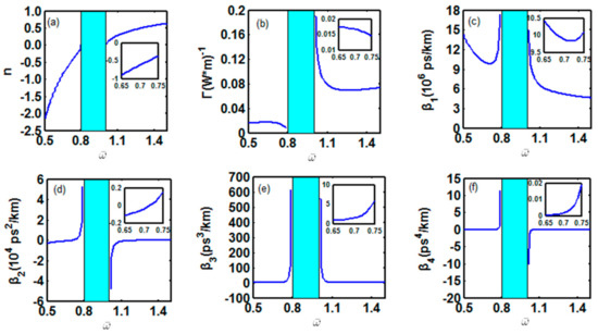
We plot the refractive index, dispersion coefficients, and third-order nonlinear coefficient in Figure 1 based on Equations (6) and (7). Although the MM structural parameters ${\omega }_{pe}$ and ${\omega }_{pm}$ can be tuned, we employ the regularly exampled parameters with third-order electric susceptibility ${\chi }^{(3)}$ as $1.9\times {10}^{-9}{ \mathrm{W}}^{-1}$ [20], ${\omega }_{pe}$ as $1.3673\times {10}^{16} \mathrm{Hz}$ [21], and ${\overline{\omega }}_p$ as 0.8 [22].

Figure 1. Variations of refractive index, third-order nonlinear coefficient, first-, second-, third-, and forth-order dispersion on $\overline{\omega }$. Insets are the magnification nearby $\overline{\omega }=0.7$.(a) Refractive index versus $\overline{\omega }$; (b) third-order nonlinear coefficient versus $\overline{\omega }$; (c) first-order dispersion versus $\overline{\omega }$; (d) second-order dispersion versus $\overline{\omega }$; (e) third-order dispersion versus $\overline{\omega }$; and (f) forth-order dispersion versus $\overline{\omega }$.

In Figure 1a, the normalized frequency can be divided into three domains, with $0<\overline{\omega }<0.8$ as the negative refractive index domain and $\overline{\omega }>1.0$ as the positive refractive index domain, respectively. The intervening region $0.8\le \overline{\omega }\le 1.0$ is the so called anomalous absorptive domain in the MM, in which the electromagnetic wave cannot propagate. It should be mentioned that (1) in Figure 1d ${\beta }_2$ increases from negative to positive in the negative refractive index region, with its zero point at ${\overline{\omega }}_D=0.706844$; (2) in Figure 1e ${\beta }_3$ is always greater than zero in both the positive and negative refractive index regions, and becomes very smooth while it is far away from the anomalous absorptive domain; (3) in Figure 1f ${\beta }_4$ is always positive in the negative refractive index region.

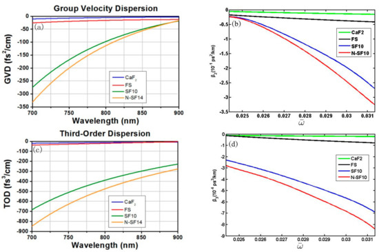
Let’s compare Figure 1 to the traditional media listed in Figure 2. Figure 2a,c, obtained from Thorlabs website [4,5], show the ${\beta }_2$ and ${\beta }_3$ of four conventional glass as a function of wavelength. In order to compare Figure 2a,c with Figure 1d,e, we need to unify the different units of abscissa in these figures. We thereby obtain Figure 2b,d by redrawing Figure 2a,c with modified abscissa and ordinate units. From Figure 2b it can be seen that ${\beta }_2$ of these conventional glass are all very small, with the order of magnitude at only ${10}^{-1}$. However, ${\beta }_2$ in Figure 1d is ${10}^4$ nearby ${\overline{\omega }}_D$. It can be estimated if extending the ${\beta }_2$ curves in Figure 2b to ${\overline{\omega }}_D$, following the current trend, the absolute value $\left|{\beta }_2\right|$ should still be smaller than that in Figure 1d. Thus, we may say that $\left|{\beta }_2\right|$ of the MM, with the regularly used ${\omega }_{pe}$ and ${\omega }_{pm}$ is much larger than that in the conventional glass. Similarly, from Figure 2d, it can be seen that ${\beta }_3$ of these conventional glass are all very small, with the order of magnitude at only ${10}^{-4}$. However, ${\beta }_3$ in Figure 1e is ${10}^0$, nearby ${\overline{\omega }}_D$. It can be estimated that, if extending the ${\beta }_3$ curves in Figure 2d to ${\overline{\omega }}_D$, following the current trend, the absolute value $\left|{\beta }_3\right|$ should still be smaller than that in Figure 1e. Therefore, we may say that $\left|{\beta }_3\right|$ of the MM with the regularly used ${\omega }_{pe}$ and ${\omega }_{pm}$ is much stronger than that in the conventional glass. What is the impact of such high dispersions in the MM? We find out these effects by studying the light pulse propagation in the MM.

Figure 2. (a,c) Second- and third-order dispersions in several conventional glass verse wavelength; (b,d) redrawing (a,c) to the normalized frequency.

4. Light Pulse Propagation in the MM

The split-step Fourier method that has been used extensively to solve the pulse-propagation problem in nonlinear dispersive media is a kind of effective beam propagation methods (BPM) [19]. We employ the split-step Fourier method to simulate the propagation of the light pulse in the MM. The incident pulse is the Gaussian pulse with $T_0$, the half pulse width at the $1/e$ of the optical peak intensity. The full width at the half maximum (FWHM) is taken to be $T_{FWHM}=5ps$ in the simulation, which is equivalent to a bit rate of $200 \mathrm{Gbps}$. The second- and third-order dispersion length are $L_D$ and ${L^{\prime }}_D$, respectively. The discussion of propagation issues requires the MM with a relatively long length. Although currently there is limitation in making long length MMs, we believe that in the near future, the technology will have breakthroughs in long length MM manufacture.

4.1. Impact of ${\beta }_2$ and ${\beta }_3$

4.1.1. Impact of ${\beta }_2$ at ${\overline{\omega }}_D$

The zero dispersion frequency ${\overline{\omega }}_D= 0.706844$ (with ${\beta }_2= 0$) in Figure 1d means the Gaussian pulse can propagate in the MM forever with no pulse spreading due to ${\beta }_2$. This is a specific phenomenon in the MM and seems an ideal circumstance. From Figure 1e, there is ${\beta }_3=2.0698 {\mathrm{ps}}^3/\mathrm{km}$ at ${\overline{\omega }}_D$. This ${\beta }_3$ is large so that the corresponding dispersion length is only ${L^{\prime }}_D=60.39 \mathrm{km}$. To have a fair idea of when and how ${\beta }_3$ takes effect, we simulate the propagation of the Gaussian pulse in Figure 3.

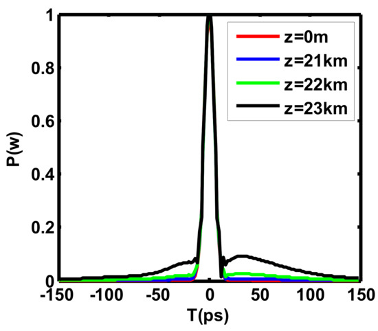
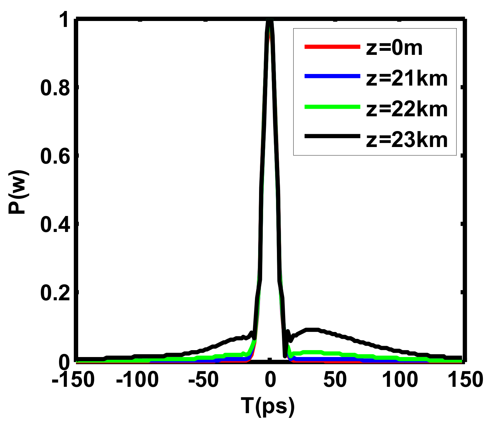
Figure 3. Pulse waveforms at different distances when ${\beta }_2=0$.

It is shown in Figure 3 that Gaussian pulse keeps its original waveform unchanged at $z<21 \mathrm{km}$. However, at around $z=22 \mathrm{km}$, the pulse starts forming a splitting peak under the influence of ${\beta }_3$. Although the pulse splitting just starts around $z=22 \mathrm{km}$, it develops quickly and has become obvious, while the pulse just transmits one more kilometer. This illustrates that ${\beta }_3$ starts to take its effect at a much earlier distance than ${L^{\prime }}_D=60.39 \mathrm{km}$, and when a pulse transmits $60.39 \mathrm{km}$, the impact of ${\beta }_3$ should be very serious, so that the original pulse waveform may be completely ruined. We have pointed out in the former section that ${\beta }_3$ in the MM is four orders of magnitude stronger than that in ordinary glass. It is such a super larger third-order dispersion that pulse splitting starts at a short distance. Thus, although an ideal circumstance of ${\beta }_2 = 0$ predicts an infinite transmission, the strong ${\beta }_3$ limits the practical transmission to a very short distance. Therefore, we need to alter our perspective by seeking an occurrence with the compensated ${\beta }_2$ and very small ${\beta }_3$. In the following two sections, we first discuss the situation nearby the zero-dispersion frequency ${\overline{\omega }}_D$.

4.1.2. Impact of ${\beta }_2$ and ${\beta }_3$ when $\overline{\omega }<{\overline{\omega }}_D$

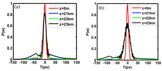
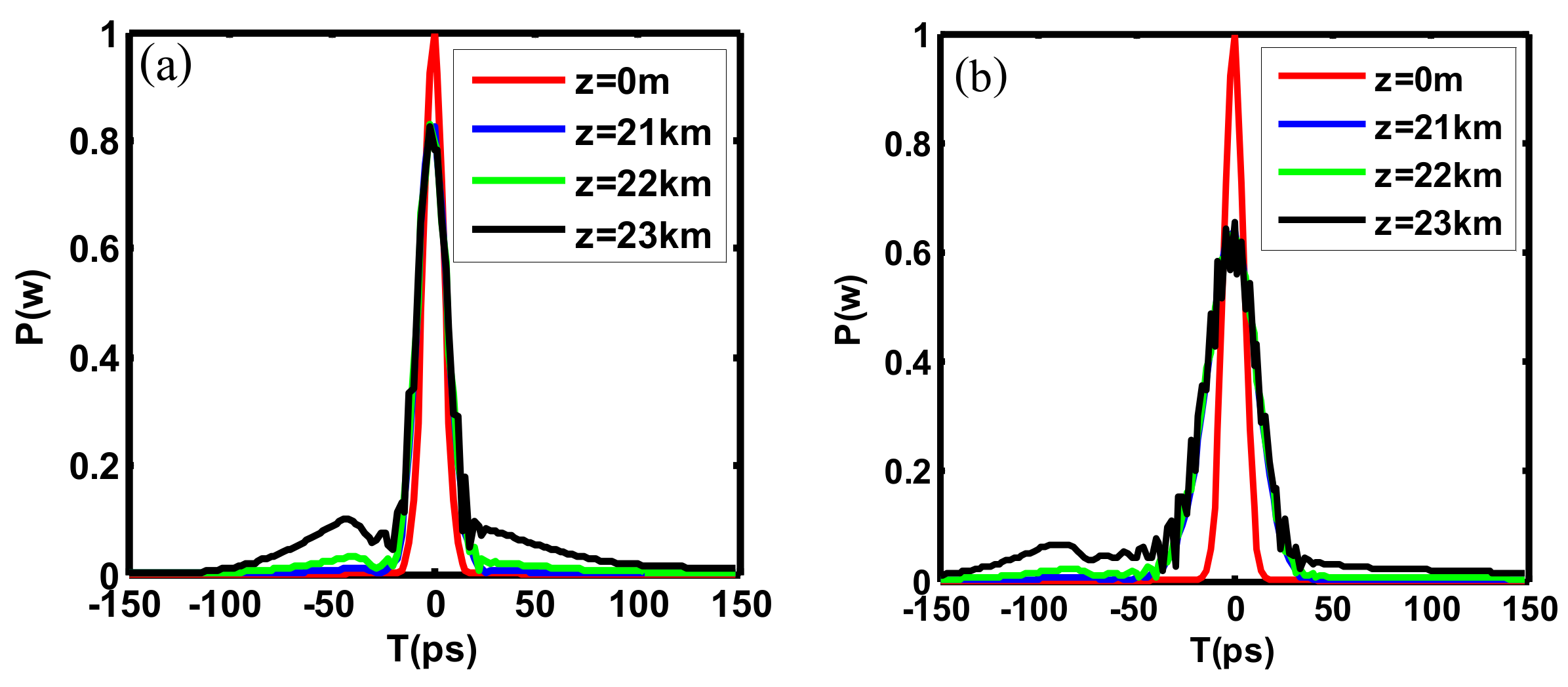
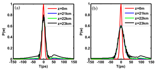
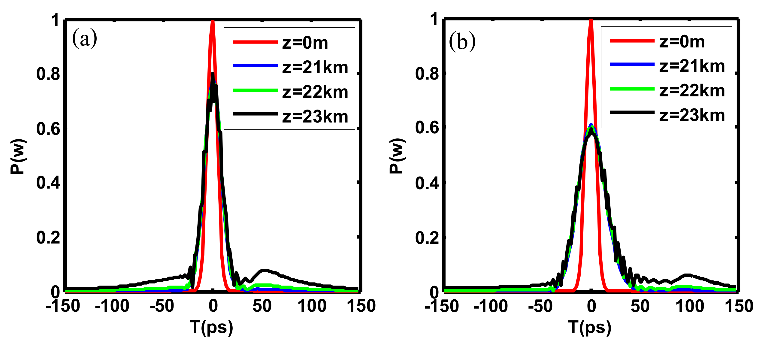
When $\overline{\omega }<{\overline{\omega }}_D$ in Figure 1d, there is ${\beta }_2<0$. Two sets of data are listed in Table 1 with different $\left|{\beta }_2\right|$ but little varied ${\beta }_3$. In addition, ${\beta }_3$ is chosen to be close to the data discussed in Section 4.1.1. Thus, ${L^{\prime }}_D$ is closed to that in the last section. Figure 4 shows the waveform plot corresponding to the two cases in Table 1. Similarly, the pulse starts to split around $z=22 \mathrm{km}$, although ${L^{\prime }}_D$ exceeds $60 \mathrm{km}$.

Table 1. Two sets of dispersion data for $\overline{\omega }<{\overline{\omega }}_D$.

$\overline{\mathit{\omega }}$	${\mathit{\beta }}_2\left({\mathbf{ps}}^2/\mathbf{km}\right)$	${\mathit{\beta }}_3\left({\mathbf{ps}}^3/\mathbf{km}\right)$	${\mathit{L}}_{\mathit{D}}\left(\mathbf{km}\right)$	${{\mathit{L}}^{\prime }}_{\mathit{D}}\left(\mathbf{km}\right)$
0.70680	−1.2589	2.0676	19.86	60.46
0.70675	−2.6715	2.0675	9.36	60.53

Figure 4. The pulse waveform comparison at different propagation distances. (a) The first case in Table 1; and (b) the second case in Table 1.

In comparison to Figure 4a,b, we can see that for the second case in Table 1, where $\left|{\beta }_2\right|$ is relatively larger, the secondary peak generated from the pulse splitting is a little far from the main peak and its peak intensity is relatively smaller. Thus, it may say that, to some extent, a larger $\left|{\beta }_2\right|$ can inhibit the influence of pulse splitting. In addition, Figure 4 also show that the secondary peak appears at the front edge of the pulse if ${\beta }_2 <0$. We also noted that the pulse splitting in Figure 4b is not so serious as that in Figure 3, although ${\beta }_3$ is similar. Again, this is due to the inhabitation of ${\beta }_2$ to the pulse splitting.

4.1.3. Impact of ${\beta }_2$ and ${\beta }_3$ when $\overline{\omega }>{\overline{\omega }}_D$

When $\overline{\omega }>{\overline{\omega }}_D$ in Figure 1d, there is ${\beta }_2>0$. Two sets of data are listed in Table 2, with different ${\beta }_2$ but little varied ${\beta }_3$. Similarly, ${\beta }_3$ is chosen to be close to the data discussed in Section 4.1.1. Figure 5 shows the waveform plot corresponding to Table 2. Similarly, the pulse starts to split around $z=22 \mathrm{km}$, although ${L^{\prime }}_D$ exceeds $60 \mathrm{km}$. The major difference between Table 1 and Table 2 is the sign of ${\beta }_2$, but ${\beta }_2$ always causes pulse broadening, no matter its sign. So, Figure 5 is similar to Figure 4. The difference is that the secondary peak appears at the rear edge of the pulse if ${\beta }_2 >0$. It also illustrates that, to some extent, a larger $\left|{\beta }_2\right|$ can inhibit the influence of the pulse splitting. We also noted that the pulse splitting in Figure 5d is not as serious as that in Figure 3, in spite of a higher ${\beta }_3$ here. Again, this is due to the inhabitation of ${\beta }_2$.

Table 2. Two sets of dispersion data for $\overline{\omega } >{\overline{\omega }}_D$.

$\overline{\mathit{\omega }}$	${\mathit{\beta }}_2\left({\mathbf{ps}}^2/\mathbf{km}\right)$	${\mathit{\beta }}_3\left({\mathbf{ps}}^3/\mathbf{km}\right)$	${\mathit{L}}_{\mathit{D}}\left(\mathbf{km}\right)$	${{\mathit{L}}^{\prime }}_{\mathit{D}}\left(\mathbf{km}\right)$
0.70690	1.5715	2.0726	15.91	60.31
0.70695	2.9894	2.0752	8.36	60.24

Figure 5. The pulse waveform comparison at different propagation distances. (a) The first case in Table 2; and (b) the second case in Table 2.

4.2. Impact of ${\beta }_2$, ${\beta }_3$, and ${\beta }_4$

In conventional media, the influence of ${\beta }_4$ can be ignored as it is so small. Section 3 shows that ${\beta }_4$ in the MM may be larger than that in the ordinary materials, however, it is just in ${10}^{-3}$ order of magnitude around ${\overline{\omega }}_D$, three orders of magnitude smaller than ${\beta }_3$ (Figure 1f). What is its impact?

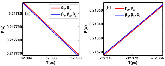
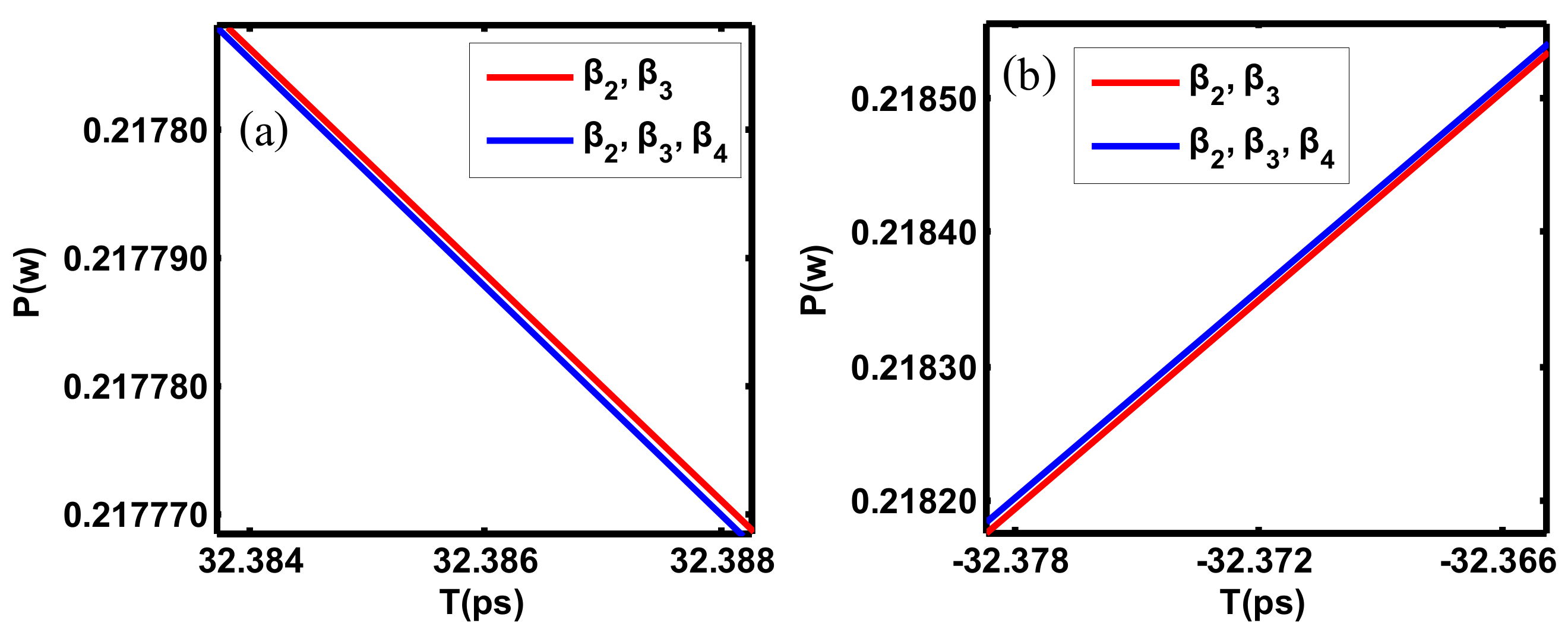
There are two groups of data in Table 3, in which $\left|{\beta }_2\right|$, ${\beta }_3$, and ${\beta }_4$ are not much different, except for the different sign for ${\beta }_2$. In Figure 6, the red line represents the portion of the pulse waveform only under the impact of ${\beta }_2$ and ${\beta }_3$, while the blue one represents the similar waveform under the simultaneous impact of ${\beta }_2$, ${\beta }_3$, and ${\beta }_4$. It is shown from a comparison to the details after the magnification of the red and blue lines at $z=21 \mathrm{km}$ that for ${\beta }_2<0$ in Figure 6a, the blue line is lower than the red line, representing a somewhat inhibition of ${\beta }_2$ to the pulse broadening, while for ${\beta }_2>0$ in Figure 6b, it is opposite, representing a little aggravation of ${\beta }_2$ to the pulse broadening. We also find that ${\beta }_4$ has no effect on the position of pulse splitting.

Table 3. Two sets of dispersion data including ${\beta }_4$.

$\overline{\mathit{\omega }}$	${\mathit{\beta }}_2\left({\mathbf{ps}}^2/\mathbf{km}\right)$	${\mathit{\beta }}_3\left({\mathbf{ps}}^3/\mathbf{km}\right)$	${\mathit{\beta }}_4\left({\mathbf{ps}}^4/\mathbf{km}\right)$	${\mathit{L}}_{\mathit{D}}\left(\mathbf{km}\right)$	${{\mathit{L}}^{\prime }}_{\mathit{D}}\left(\mathbf{km}\right)$
0.706587	−7.2648	2.0569	0.0037	3.44	60.77
0.70710	7.2532	2.0828	0.0037	3.45	60.02

Figure 6. Magnification of the partial propagation waveform at FWHM for $z=21 \mathrm{km}$. (a) The first case in Table 3; and (b) the second case in Table 3.

5. Dispersion Management in MMs

5.1. Design of the Optimal Dispersion

From the above analyses, it is realized that the second- and third-order dispersions are all serious for that particular MM, which is often exampled in the literature with ${\omega }_{pe}=1.3673\times {10}^{16}\mathrm{Hz}$ and ${\overline{\omega }}_p=0.8$ [21,22]. This makes the propagation with $z>22 \mathrm{km}$ impossible. However, MMs are such extraordinary materials that derive their properties not only from the properties of the base materials, but from their newly artificially designed structures. Their precise shape, geometry, size, orientation, and arrangement give them their smart properties capable of manipulating electromagnetic waves to achieve benefits that go beyond what is possible with conventional materials. Therefore, we expand on our views to other MMs with different ${\omega }_{pe}$ and ${\omega }_{pm}$ (i.e., ${\overline{\omega }}_p$), and take insight into the dependence of dispersion to the structural parameters ${\omega }_{pe}$ and ${\omega }_{pm}$. To obtain small second- and third-order dispersions for a reasonably long transmission, we present here the design of an MM by using the nano-inclusions model [23], made of properly arranged collections of plasmonic metallic nano-rings.

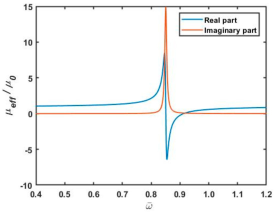
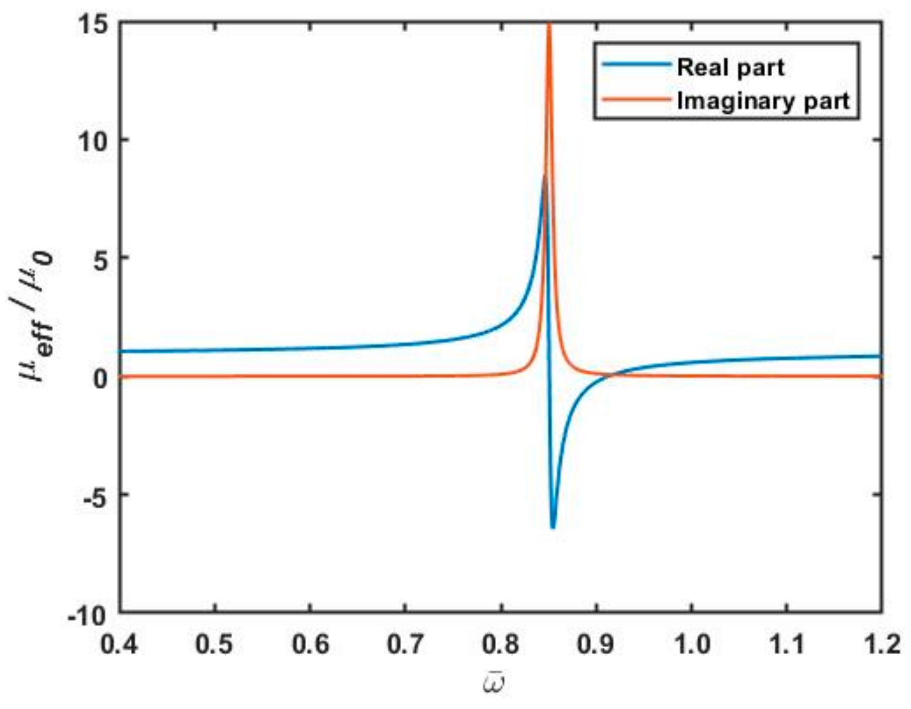
In our design, the nano-rings are made of a typical metal like aluminum, with its electrical plasma frequency described by ${\omega }_{pe}=\sqrt{N{q}_e^2/\left(m{\epsilon }_0\right)}$, where N is the density of electrons, $q_e$ is the electron charge, m is the electron mass, and ε₀ is the dielectric permittivity in a vacuum [24]. For aluminum, the number of electrons per cubic meter can be $N=1.806\times {10}^{29}{\mathrm{m}}^{-3}$ [16], then, there is ${\omega }_{pe}=2.396\times {10}^{16}\mathrm{Hz}$. When such aluminum nano-rings are embedded in a host medium, they may provide metamaterials with negative effective permeability at optical frequencies. According to the nano-inclusions model by the authors of [23], we calculated the effective permeability for the periodic arrangement of the aluminum nano-rings. The resonant magnetic dipole collective response of the effective permeability is presented in Figure 7, with R = 40 nm, a = 16 nm, N = 6, and N_d = (108 nm)⁻³. Following [25,26], the damping frequency and high frequency dielectric constant of aluminum have been assumed to follow the Drude model with ${\omega }_{\tau }=194 \mathrm{THz}$ and ${\epsilon }_{\infty }=1.65{\epsilon }_0$. The background material in this design is ${\epsilon }_b=1.2{\epsilon }_0$. With the effective magnetic permeability, the magnetic plasma frequency ${\omega }_{pm}$ can be obtained following the Drude model.

Figure 7. Effective relative magnetic permeability for bulk medium with the geometry of nano-rings.

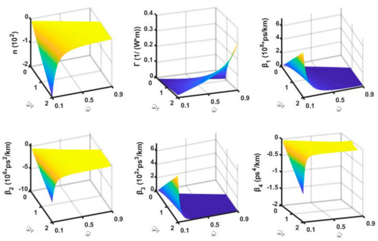
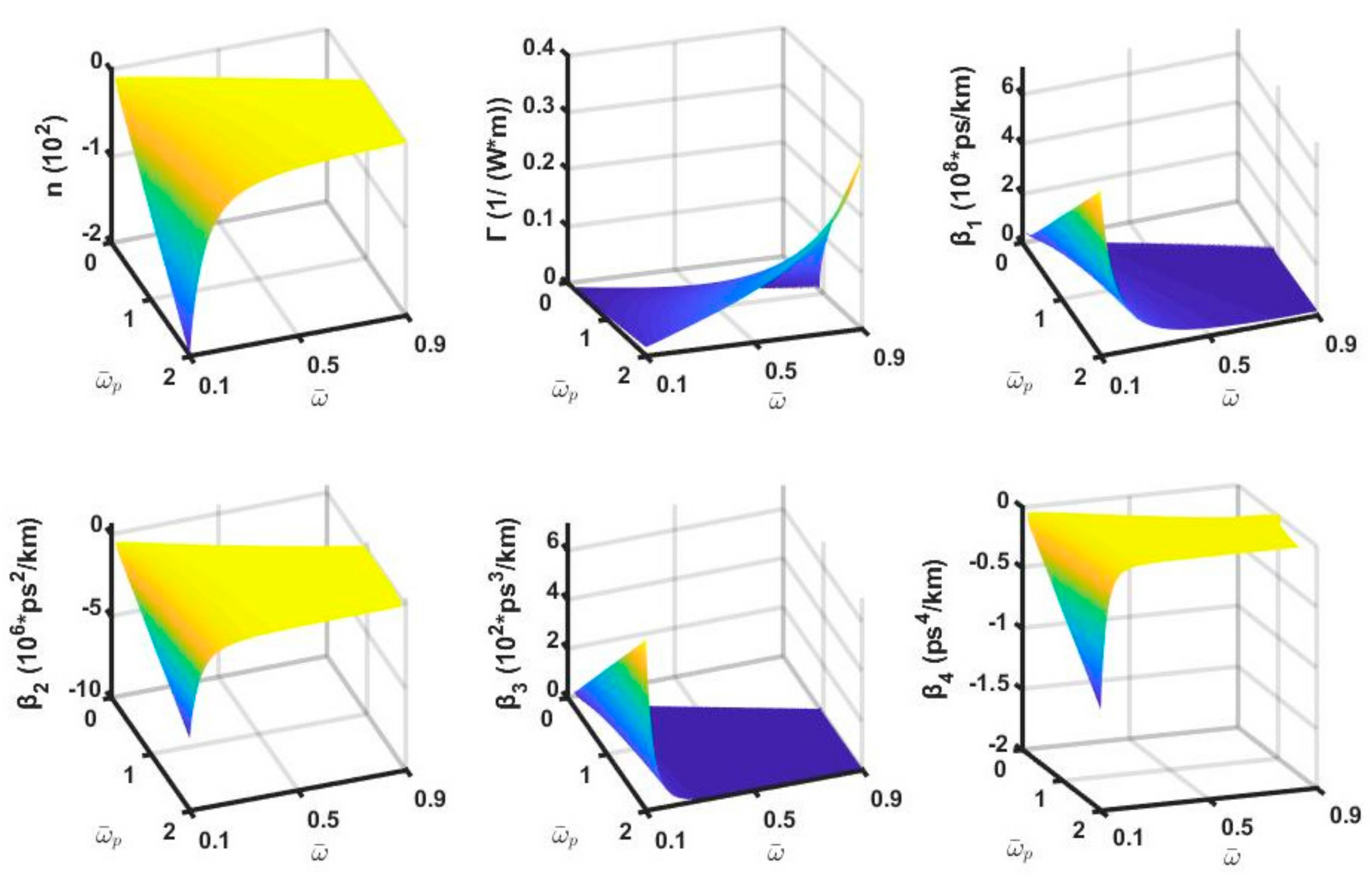
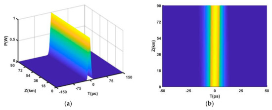
Using Equation (6), we also obtained a group of 3D plots in Figure 8 for $0.1\le \overline{\omega }\le 0.9$ and $0.1\le {\overline{\omega }}_p\le 2$, with the fixed ${\omega }_{pe}=2.396\times {10}^{16}\mathrm{Hz}$. According to the definition, the range of ${\overline{\omega }}_p$ here, gives out the range of ${\omega }_{pm}$. We search in Figure 8 for all of the values of ${\omega }_{pm}$ gained from our above design to check up their dispersion parameters, and hope to find the potential figures with lower dispersions. We pick out all points with approximately zero ${\beta }_2$ and very low ${\beta }_3$. Forty eight points with the second-order dispersion length $L_D>525 \mathrm{km}$ and the third-order dispersion length ${L^{\prime }}_D\approx 290 \mathrm{km}$ are found (see Appendix A). Among them, the best three points with the longest ${L^{\prime }}_D$ and an extremely low second-order dispersion are listed in Table 4. Figure 9 is an example of $90 \mathrm{km}$ of a repeaterless transmission for the second group of data in Table 4. Within this distance, there is almost no expansion due to group-velocity dispersion (GVD) and any impact from third-order dispersion whose impact emerges while $z\ge 90 \mathrm{km}$. Although we point out that the MM with ${\omega }_{pe}=1.3673\times {10}^{16} \mathrm{Hz}$ and ${\overline{\omega }}_p=0.8$ [21,22] exhibits serious dispersion, it is delightful to see the MM we designed is not incurable in dispersion and can be employed for long distance transmission in the future, when long-length MMs are ready.

Figure 8. Dependence of refractive index, third-order nonlinear coefficient, first-, second-, third-, and forth-order dispersion on $\overline{\omega }$ and ${\overline{\omega }}_p$, with ${\omega }_{pe}=2.396\times {10}^{16}\mathrm{Hz}$.

Table 4. Examples for the lowest second- and third-order dispersions with ${\omega }_{pe}=2.396\times {10}^{16}\mathrm{Hz}$.

$\overline{\mathit{\omega }}$	${\overline{\mathit{\omega }}}_{\mathit{p}}$	${\mathit{\omega }}_{\mathit{p}\mathit{m}}\times {10}^{16}\left(\mathit{H}\mathit{z}\right)$	${\mathit{\beta }}_2\left({\mathbf{ps}}^2/\mathbf{km}\right)$	${\mathit{\beta }}_3\left({\mathbf{ps}}^3/\mathbf{km}\right)$	${\mathit{\beta }}_4\left({\mathbf{ps}}^4/\mathbf{km}\right)$	${\mathit{L}}_{\mathit{D}}\left(\mathbf{km}\right)$	${{\mathit{L}}^{\prime }}_{\mathit{D}}\left(\mathbf{km}\right)$
0.8794313	1.277639	3.061222	0.002528	0.431002	0.0003325	9889.982	290.0218
0.8794314	1.277637	3.0612173	0.000674	0.431001	0.0003325	37111.35	290.0227
0.8794315	1.277635	3.0612125	−0.00118	0.430999	0.0003325	21177.19	290.0237

Figure 9. (a) Gaussian pulse’s 90 km propagation; (b) top view of (a).

5.2. Dispersion Management

Dispersion compensation is for the circumstance in which ${\beta }_2$ and ${\beta }_3$ can both be compensated or ${\beta }_2$ is compensated, but ${\beta }_3$ is very small. According to the dispersion compensation theory, to reach the compensation for both ${\beta }_2$ and ${\beta }_3$, there should be the following [19]:

$${\beta }_{21}{L}_1+{\beta }_{22}{L}_2=0\begin{array}{ccc}& & {\beta }_{31}{L}_1+{\beta }_{32}{L}_2=0\end{array}$$

(11)

where $L=L_1+L_2$ is dispersion period, ${\beta }_{2j}$ and ${\beta }_{3j}$ (j = 1, 2) are second- and third-order dispersion for the MM with length $L_j$.

Figure 8d shows that ${\beta }_2$ can be positive and negative, so there is a possibility to reach ${\beta }_2$ compensation. However, in Figure 8e, ${\beta }_3$ is always positive, meaning that we cannot find a negative valued ${\beta }_3$ to reach its compensation. Luckily, for the same normalized frequencies we found two sets of data in Table 5 with an opposite notation and very closed absolute values of ${\beta }_2$ for compensation. Additionally, both sets of data all have very low ${\beta }_3$, resulting in ${L^{\prime }}_D$ as long as $380 \mathrm{km}$. That is to say, while the broadening due to the GVD is compensated, the effect due to the third-order dispersion has not yet emerged. Thus, we propose a configuration with metamaterials MM1 and MM2, cross-linked periodically with their length $L_1=L_2=20 \mathrm{km}$. The simulation results for the propagation of the Gaussian pulse in the composite metamaterial MM1 and MM2 is demonstrated in Figure 10.

Table 5. Two sets of data for ${\beta }_2$ compensation with ${\omega }_{pe}=3.3673\times {10}^{16}\mathrm{Hz}$.

Metamaterial	$\overline{\mathit{\omega }}$	${\overline{\mathit{\omega }}}_{\mathit{p}}$	${\mathit{\beta }}_2\left({\mathbf{ps}}^2/\mathbf{km}\right)$	${\mathit{\beta }}_3\left({\mathbf{ps}}^3/\mathbf{km}\right)$	${\mathit{L}}_{\mathit{D}}\left(\mathbf{km}\right)$	${{\mathit{L}}^{\prime }}_{\mathit{D}}\left(\mathbf{km}\right)$
MM1	0.88	0.941095	1.184911	0.330214	21.10	378.56
MM2	0.88	0.941240	−1.183498	0.327182	21.12	382.03

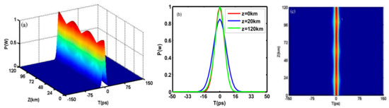
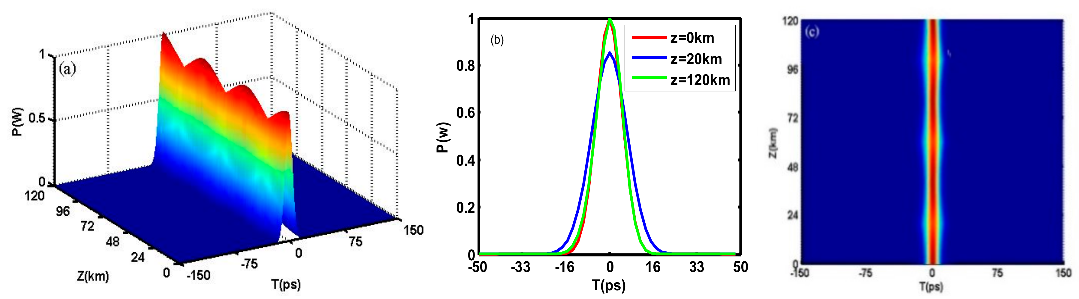
Figure 10. (a) Gaussian pulse’s 120 km propagation in MM1 and MM2; (b) waveforms of the Gaussian pulse; (c) top view of (a).

Figure 10 shows that when the pulse transmits in MM1, its width spreads with the increase of the propagation distance, and the pulse intensity lowers because of the pulse broadening. At the propagation distance $L_1=20 \mathrm{km}$, the pulse intensity reduces 20%. At this time, if we let the pulse enter into MM2 and it continually transmits inside MM2, the reduced intensity starts to be recovered and the broadened width gradually shrinks. At $Z=L_1+L_2=20+20=40 \mathrm{km}$, the intensity and the width have both been recovered to be equivalent to their initial values. The situation afterwards repeats the first MM1 and MM2 period, until it transmits $Z=120 \mathrm{km}$. While the pulse transmits one MM1 and MM2 period, the impact of ${\beta }_3$ remains uncompensated and accumulates with the increment of the transmission distance. The simulation shows that while the propagation distance approaches $140 \mathrm{km}$, the pulse splitting due to ${\beta }_3$ starts to emerge. Therefore, the MM1 and MM2 cross-linked structure allows a $120 \mathrm{km}$ repeaterless transmission.

6. Conclusions

The paper studies the dispersion in MMs and finds that the GVD and higher order dispersion in MMs may often be much more serious than that in conventional glass. Since obtaining optical properties on demand by reconfiguring the MM constitutes and structure has not been unreachable, we may be able to design MMs and obtain the dispersive properties at extensive electric and magnetic plasma frequency ranges with desire. Thus, we investigate the relationship of dispersion with the MM structural parameters ${\omega }_{pe}$ and ${\omega }_{pm}$, propose two approaches with the optimal dispersion through the MM design and the composite metamaterial MM1 and MM2 for dispersion management, and demonstrate 90 km and 120 km long distance successful transmission, respectively.

References

- Born, M.; Wolf, E. Princiiples of Optics; Cambridge University Press: Cambridge, UK, 1999; pp. 14–24. [Google Scholar]
- Shelby, R.A.; Smith, D.R.; Shultz, S.; Nemat-Nasser, S.C. Microwave transmission through a two-dimensional, isotropic, left-handed metamaterial. Appl. Phys. Lett. 2001, 78, 489–491. [Google Scholar] [CrossRef] [Scilit]
- Smith, D.R.; Padilla, W.J.; Vier, D.C.; Nemat-Nasser, S.C.; Schultz, S. Composite Medium with Simultaneously Negative Permeability and Permittivity. Phys. Rev. Lett. 2000, 84, 4184–4187. [Google Scholar] [CrossRef] [Scilit] [PubMed]
- Group Velocity Dispersion. Available online: https://www.thorlabs.us/images/TabImages/ AFS_prisms_GVD_G2-480.gif (accessed on 22 February 2018).
- Third Order Dispersion. Available online: https://www.thorlabs.us/images/TabImages/ AFS_prisms_TOD_G2-480.gif (accessed on 22 February 2018).
- Smith, D.R.; Pendry, J.B.; Wiltshire, M.C.K. Metamaterials and negative refractive index. Science 2004, 305, 788–792. [Google Scholar] [CrossRef] [Scilit] [PubMed]
- Engheta, R.; Ziolkowski, R.W. Metamaterials, Physics and Engineering Explorations; Wiley-IEEE: New York, NY, USA, 2006. [Google Scholar]
- Shalaev, V.M. Optical negative-index metamaterials. Nat. Photonics 2007, 1, 41–48. [Google Scholar] [CrossRef] [Scilit]
- Liu, Y.; Zhang, X. Metamaterials: A new frontier of science and technology. Chem. Soc. Rev. 2011, 40, 2494–2507. [Google Scholar] [CrossRef] [Scilit] [PubMed]
- Soukoulis, C.M.; Wegener, M. Past achievements and future challenges in the development of three-dimensional photonic metamaterials. Nat. Photonics 2011, 5, 523–530. [Google Scholar] [CrossRef] [Scilit]
- Zheludev, N.I.; Kivshar, Y.S. From metamaterials to metadevices. Nat. Mater. 2012, 11, 917–924. [Google Scholar] [CrossRef] [Scilit] [PubMed]
- Zheludev, N.I.; Plum, E. Reconfigurable nanomechanical photonic metamaterials. Nat. Nanotechnol. 2016, 11, 16–22. [Google Scholar] [CrossRef] [Scilit] [PubMed]
- Zheludev, N.I. Obtaining optical properties on demand. Science 2015, 348, 973–974. [Google Scholar] [CrossRef] [Scilit] [PubMed]
- Dastmalchi, B.; Tassin, P.; Koschny, T.; Soukoulis, C.M. Strong group-velocity dispersion compensation with phase-engineered sheet metamaterials. Phys. Rev. B 2014, 89, 115123. [Google Scholar] [CrossRef] [Scilit]
- Veselago, V.G. Electrodynamics of substances with simultaneously negative electrical and magnetic permeabilities. Sov. Phys. Usp. 1968, 10, 504–509. [Google Scholar] [CrossRef] [Scilit]
- Pendry, J.B.; Holden, A.J.; Stewart, W.J.; Youngs, I. Extremely Low Frequency Plasmons in Metallic Mesostructures. Phys. Rev. Lett. 1996, 76, 4773–4776. [Google Scholar] [CrossRef] [Scilit] [PubMed]
- Pendry, J.B.; Holden, A.J.; Robbins, D.J.; Stewart, W.J. Magnetism from conductors and enhanced nonlinear phenomena. IEEE Trans Microw. Theory Tech. 1999, 47, 2075–2084. [Google Scholar] [CrossRef] [Scilit]
- Shelby, R.A.; Smith, D.R.; Schultz, S. Experimental verification of a negative index of refraction. Science 2011, 292, 77–79. [Google Scholar] [CrossRef] [Scilit] [PubMed]
- Agrawal, G.P. Nonlinear Fiber Optics, 5th ed.; Academic Press: Cambridge, MA, USA, 2013. [Google Scholar]
- Liu, Y.; Xue, Y.L.; Yu, C. Modulation instability induced by cross-phase modulation in negative index materials with higher-order nonlinearity. Opt. Commun. 2015, 339, 66–73. [Google Scholar] [CrossRef] [Scilit]
- Shalaev, V.M.; Cai, W.; Chettiar, U.K.; Yuan, H.; Sarychev, A.K.; Drachev, V.P.; Kildishev, A.V. Nagative index of refraction in optical metamaterials. Opt. Lett. 2005, 30, 3356–3358. [Google Scholar] [CrossRef] [Scilit] [PubMed]
- Wen, S.; Wang, Y.; Su, W.; Xiang, Y.; Fu, X.; Fan, D. Modulation instability in nonlinear negative-index material. Phys. Rev. E 2006, 73, 036617. [Google Scholar] [CrossRef] [Scilit] [PubMed]
- Alù, A.; Salandrino, A. Negative effective permeability and left-handed materials at optical frequencies. Opt. Express 2006, 14, 1557–1567. [Google Scholar] [CrossRef] [Scilit] [PubMed]
- YXue, L.; Liu, W.; Gu, Y.; Zhang, Y. Light storage in a cylindrical waveguide with metamaterials. Opt. Laser Technol. 2015, 68, 28–35. [Google Scholar]
- Ordal, M.A.; Bell, R.J.; Alexander, R.W., Jr.; Long, L.L.; Querry, M.R. Optical properties of fourteen metals in the infrared and far infrared: Al, Co, Cu, Au, Fe, Pb, Mo, Ni, Pd, Pt, Ag, Ti, V, and W. Appl. Opt. 1985, 24, 4493–4499. [Google Scholar] [CrossRef] [Scilit] [PubMed]
- Ordal, M.A.; Long, L.L.; Bell, R.J.; Bell, S.E.; Bell, R.R.; Alexander, R.W.; Ward, C.A. Optical properties of the metals Al, Co, Cu, Au, Fe, Pb, Ni, Pd, Pt, Ag, Ti, and W in the infrared and far infrared. Appl. Opt. 1983, 22, 1099–1119. [Google Scholar] [CrossRef] [Scilit] [PubMed]
© 2018 by the authors. Licensee MDPI, Basel, Switzerland. This article is an open access article distributed under the terms and conditions of the Creative Commons Attribution (CC BY) license (http://creativecommons.org/licenses/by/4.0/).