L₁ Adaptive Control for a Vertical Rotor Orientation System

Abstract

Bottom-fixed vertical rotating devices are widely used in industrial and civilian fields. The free upside of the rotor will cause vibration and lead to noise and damage during operation. Meanwhile, parameter uncertainties, nonlinearities and external disturbances will further deteriorate the performance of the rotor. Therefore, in this paper, we present a rotor orientation control system based on an active magnetic bearing with $L_1$ adaptive control to restrain the influence of the nonlinearity and uncertainty and reduce the vibration amplitude of the vertical rotor. The boundedness and stability of the adaptive system are analyzed via a theoretical derivation. The impact of the adaptive gain is discussed through simulation. An experimental rig based on dSPACE is designed to test the validity of the rotor orientation system. The experimental results show that the relative vibration amplitude of the rotor using the $L_1$ adaptive controller will be reduced to ∼50% of that in the initial state, which is a 10% greater reduction than can be achieved with the nonadaptive controller. The control approach in this paper is of some significance to solve the orientation control problem in a low-speed vertical rotor with uncertainties and nonlinearities.

1. Introduction

Vertical rotation devices are widely applied in industrial, scientific and civilian fields, e.g., flywheels, centrifuges and washing machines. Many of these applications have a fixed bottom bearing with a free upper side. The one-side bearing structure will lead to vibration during operation and, consequently, cause collision, noise and failure. One of the traditional methods to solve this problem in washing machines is through the addition of a passive balancer [1,2,3]. However, passive control approaches, although having the advantages of simplicity and low cost, are unsatisfactory in vibration reduction because of their open-loop property. For the vertical rotation devices, an active non-contacted vibration reduction system, such as an active magnetic bearing (AMB), placed at the upper side to control the attitude of the rotor, offers a better solution to the vibration problem.

The Active Magnetic Bearing (AMB) system is a nonlinear system, with many uncertainties during its operation, such as parameter uncertainty and external random disturbances. Therefore, the control of the AMB system has been an active research topic. For example, [4] presented a feedback linearization approach to control the position of a horizontal rotor; [5], aiming at a 1-kWh flywheel energy storage device, analyzed the advantages and disadvantages of different approaches, such as decentralized control, Linear Quadratic Regulator (LQR) control and cross-feedback control; [6] proposed an on-line parameter identification method to solve the situation in which the rotor mass is unbalanced; [7], based on an AMB test rig, used radial basis function networks to identify the uncertainties and to synthesize an $H_{\infty }$ controller with the rotor setpoint; [8] presented an adaptive back-stepped controller for a flywheel energy storage system; [9] designed a test rig consisting of a flexible rotor supported by AMBs with a $\mathsf{\mu }-$synthesis controller.

The research above mostly focused on AMBs for horizontal rotors. Research on a vertical rotor has been rather limited. For example, [10] presented an H${}^{\infty }$ controller to regulate the rotor position for vertical AMB systems under 10K rpm. This research, for either horizontal or vertical rotors, has focused on high-speed rotors. However, as mentioned above, vertical low-speed rotating devices are widely used, and their dynamic behaviors will be rather complicated [11]. Therefore, it is necessary to propose a control approach for low-speed vertical rotor position control. Meanwhile, under a lower spinning rate, the influences from parameter uncertainties and external disturbances will be more severe.

The $L_1$ adaptive control theory [12] provides a powerful tool to overcome the problems of uncertainties and nonlinearities. This theory has been utilized in many applications, e.g., [13] presented a one-output drilling direction adaptive control system in the presence of time-delay, unexpected disturbance and other uncertainties; [14] proposed an underactuated robots control system with unmodeled dynamics. These studies have provided significant theoretical and simulation results for $L_1$ adaptive controllers. Based on these studies, in this paper, the authors propose an $L_1$ adaptive controller for a two-input-two-output vertical rotor orientation control system and design an experimental rig based on dSPACE to test the performance of the rotor orientation control system. The work in this paper may also be applied to twin-rotor mechanical system control [15,16,17,18].

This paper is organized as follows. Section 2 establishes the mathematical model of the rotor and presents the control aim of the system. Section 3 proposes the architecture of the adaptive control system. Section 4 analyzes the stability and performance of the adaptive control system. Section 5 gives the simulation of the adaptive control system. Section 6 presents an experimental validation of the performance of the rotor orientation control system. Section 7 provides a summary of the work.

2. Problem Statement

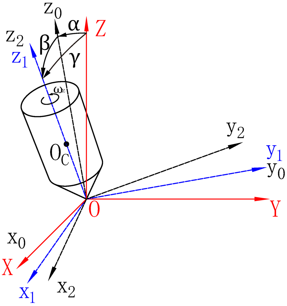
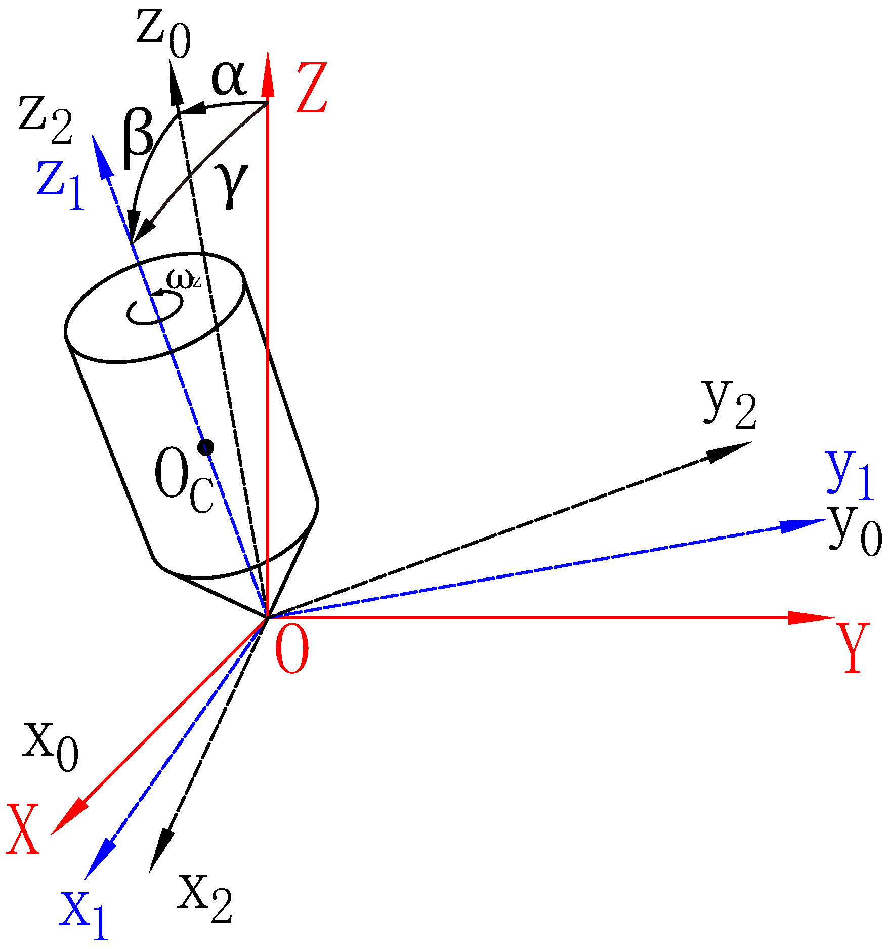
The vertical rotor is shown in Figure 1. α and β are the attitude angles of the rotor from $OXZ$ and $OYZ$, respectively. γ is the included angle between the rotor axis and $OZ$.

Figure 1. Rotor scheme.

According to the theorem of angular momentum, the motion of the rotor satisfies:

$${\displaystyle \frac{\mathrm{d}}{\mathrm{d}t}}\mathit{L}=\mathit{T}$$

where $\mathit{L}$ is the angular momentum of the rotor and $\mathit{T}$ is the external torque.

The torque induced by the gravity is given by:

$$\left\{\begin{array}{cc}\hfill T_{xg}& =Pcsin\alpha cos\beta \hfill \\ \hfill T_{yg}& =Pcsin\beta \hfill \\ \hfill T_{zg}& =0\hfill \end{array}\right.$$

(1)

where $P=m\mathrm{g}$ is the gravitational force on the rotor; $c={\overrightarrow{OO}}_c$. Then, the state equation of a spinning vertical rotor can be written as:

$$\left\{\begin{array}{cc}\hfill {\dot{x}}_1& ={\displaystyle \frac{x_3}{cos{x}_2}}\hfill \\ \hfill {\dot{x}}_2& =x_4\hfill \\ \hfill {\dot{x}}_3& ={\displaystyle \frac{Pc}{J_{xy}}}sin{x}_{1}cos{x}_2-{\displaystyle \frac{L}{J_{xy}}}{x}_4+x_3{x}_{4}tan{x}_2+{\displaystyle \frac{T_{x\mathrm{e}}}{J_{xy}}}\hfill \\ \hfill {\dot{x}}_4& ={\displaystyle \frac{Pc}{J_{xy}}}sin{x}_2-x_3^{2}tan{x}_2+{\displaystyle \frac{L}{J_{xy}}}{x}_3+{\displaystyle \frac{T_{x\mathrm{e}}}{J_{xy}}}\hfill \end{array}\right.$$

(2)

where $x_1=\alpha$ and $x_2=\beta$; $L=J_z{\omega }_z$ is the rotor angular momentum; $J_{xy}$ and $J_z$ are the rotational inertia about the $OX/OY$ axis and the $OZ$ axis, respectively; ${\omega }_z$ is the spinning rate of the rotor; $T_{x\mathrm{e}}$ and $T_{y\mathrm{e}}$ are the external control torques in the $OX$ and $OY$ directions, respectively.

If we define the following variables:

$$\left\{\begin{array}{cc}\hfill h_1(\mathit{x})& ={\displaystyle \frac{x_3}{cos{x}_2}}\hfill \\ \hfill h_2(\mathit{x})& =x_4\hfill \\ \hfill h_3(\mathit{x})& ={\displaystyle \frac{Pc}{J_{xy}}}sin{x}_{1}cos{x}_2-{\displaystyle \frac{L}{J_{xy}}}{x}_4+x_3{x}_{4}tan{x}_2\hfill \\ \hfill h_4(\mathit{x})& ={\displaystyle \frac{Pc}{J_{xy}}}sin{x}_2-x_3^{2}tan{x}_2+{\displaystyle \frac{L}{J_{xy}}}{x}_3\hfill \end{array}\right.$$

(3)

and $\mathit{h}(\mathit{x})={\left[h_1{h}_2{h}_3{h}_4\right]}^{\top }$, then Equation (2) can be rewritten as:

$$\dot{\mathit{x}}=\mathit{h}(\mathit{x})+{\mathit{B}}_1\mathit{u}$$

(4)

where $\mathit{x}={\left[x_1{x}_2{x}_3{x}_4\right]}^{\top }$ is the state vector, $\mathit{u}={\left[T_{x\mathrm{e}}{T}_{y\mathrm{e}}\right]}^{\top }$ is the system input and:

$${\mathit{B}}_1=\left[\begin{array}{cc}0& 0\\ 0& 0\\ {\displaystyle \frac{1}{J_{xy}}}& 0\\ 0& {\displaystyle \frac{1}{J_{xy}}}\end{array}\right]$$

Obviously, $\mathit{h}(\mathbf{0})=\mathbf{0}$.

Equation (4) is a nonlinear equation. Meanwhile, parameter uncertainties also exist, e.g., the rotational inertia about the $OX/OY$ axis, $J_{xy}$, is difficult to calculate accurately, and $J_z$ in $L=J_z{\omega }_z$, as well.

Without loss of generality, we suppose that $J_{xy}=J_{xy0}+{\theta }_1$, $J_z=J_{z0}+{\theta }_2$, where $J_{xy0}$ and $J_{z0}$ are nominal moments of inertia of the rotor and ${\theta }_1$ and ${\theta }_2$ are unknown constants referred to the inertia errors. These errors include the manufacturing error and accessory connections. By considering the unknown parameters, the two elements $\mathit{h}(\mathit{x})$ and $\mathit{B}$ in Equation (4) can be written as:

$$\mathit{h}(\mathit{x})=(\mathit{A}+{\mathit{A}}_{\theta })\mathit{x}+{\mathit{f}}_1(\mathit{x}){\mathit{B}}_1=\mathit{B}+{\mathit{B}}_{\theta }$$

(5)

where:

$$\mathit{A}+{\mathit{A}}_{\theta }={\left.{\displaystyle \frac{\partial \mathit{h}}{\partial \mathit{x}}}\right|}_{\mathit{x}=\mathbf{0}}$$

represents the linear parts of $\mathit{h}(\mathit{x})$, ${\mathit{f}}_1(\mathit{x})=\mathit{h}(\mathit{x})-(\mathit{A}+{\mathit{A}}_{\theta })\mathit{x}$ represents the high-order nonlinear parts of $\mathit{h}(\mathit{x})$, while $\mathit{B}$ and ${\mathit{B}}_{\theta }$ represent the certain and uncertain part of ${\mathit{B}}_1$. The subscript θ in Equation (5) refers to the uncertain parameters. $\mathit{A}$, ${\mathit{A}}_{\theta }$, $\mathit{B}$ and ${\mathit{B}}_{\theta }$ are:

$$\mathit{A}=\left[\begin{array}{cccc}0& 0& 1& 0\\ 0& 0& 0& 1\\ {\displaystyle \frac{Pc}{J_{xy0}}}& 0& 0& -{\displaystyle \frac{J_{z0}{\omega }_z}{J_{xy0}}}\\ 0& {\displaystyle \frac{Pc}{J_{xy0}}}& {\displaystyle \frac{J_{z0}{\omega }_z}{J_{xy0}}}& 0\end{array}\right]$$

$${\mathit{A}}_{\theta }=\left[\begin{array}{cccc}0& 0& 0& 0\\ 0& 0& 0& 0\\ -{\displaystyle \frac{Pc{\theta }_1}{J_{xy0}(J_{xy0}+{\theta }_1)}}& 0& 0& -{\displaystyle \frac{{\omega }_z(J_{xy0}{\theta }_2-J_{z0}{\theta }_1)}{J_{xy0}(J_{xy0}+{\theta }_1)}}\\ 0& -{\displaystyle \frac{Pc{\theta }_1}{J_{xy0}(J_{xy0}+{\theta }_1)}}& {\displaystyle \frac{{\omega }_z(J_{xy0}{\theta }_2-J_{z0}{\theta }_1)}{J_{xy0}(J_{xy0}+{\theta }_1)}}& 0\end{array}\right]$$

$$\mathit{B}=\left[\begin{array}{cc}0& 0\\ 0& 0\\ {\displaystyle \frac{1}{J_{xy0}}}& 0\\ 0& {\displaystyle \frac{1}{J_{xy0}}}\end{array}\right],{\mathit{B}}_{\theta }=\left[\begin{array}{cc}0& 0\\ 0& 0\\ -{\displaystyle \frac{{\theta }_1}{J_{xy0}(J_{xy0}+{\theta }_1)}}& 0\\ 0& -{\displaystyle \frac{{\theta }_1}{J_{xy0}(J_{xy0}+{\theta }_1)}}\end{array}\right]$$

Next, we define:

$$\mathit{f}(t,\mathit{x}(t))={\mathit{f}}_1(\mathit{x})+{\mathit{A}}_{\theta }\mathit{x}(t)+{\mathit{B}}_{\theta }\mathit{u}(t)$$

(6)

and

$$\mathit{u}={\mathit{u}}_{\mathrm{m}}+{\mathit{u}}_{\text{ad}}$$

(7)

where ${\mathit{u}}_{\mathrm{m}}=-{\mathit{K}}_{\mathrm{m}}\mathit{x}(t)$ is a linear state feedback that renders ${\mathit{A}}_{\mathrm{m}}\triangleq \mathit{A}-\mathit{B}{\mathit{K}}_{\mathrm{m}}$ Hurwitz. ${\mathit{u}}_{\text{ad}}$ is the adaptive input vector used to compensate for the unknown parameter, system nonlinearity and other disturbances. Then, Equation (4) can be rewritten as:

$$\dot{\mathit{x}}(t)=\mathit{A}\mathit{x}(t)+\mathit{B}({\mathit{u}}_{\mathrm{m}}+{\mathit{u}}_{\text{ad}})+\mathit{f}(t,\mathit{x}(t))\mathit{x}(0)={\mathit{x}}_0$$

(8)

$\mathit{f}(t,\mathit{x})$ should satisfies the following two assumptions:

Assumption 1. 

(Uniform boundedness of $\mathit{f}(\mathit{t},\mathbf{0})$).

For any $t\ge 0$, there exists $F>0$, such that $\mathit{f}(t,\mathbf{0})\le F$.

Assumption 2. 

(Boundedness of partial derivatives).

For arbitrary $\delta >0$, there exist $d_{f_x}(\delta )$ and $d_{f_t}(\delta )$, such that, for arbitrary $\mathit{x}$, as long as ${∥\mathit{x}∥}_{\infty }\le \delta$, the partial derivatives of $\mathit{f}(t,\mathit{x})$ are bounded:

$${∥{\displaystyle \frac{\partial \mathit{f}}{\partial \mathit{x}}}∥}_{\infty }\le d_{f_x}(\delta ),{∥{\displaystyle \frac{\partial \mathit{f}}{\partial t}}∥}_1\le d_{f_t}(\delta )$$

(9)

In this paper, the system equilibrium $\mathit{x}=\mathbf{0}$ implies that the rotor is along the vertical direction, which is just the control aim of the system. In other words, the control input must ensure that the equilibrium of Equation (8) is $\mathit{x}=\mathbf{0}$. While the rotor lies vertically, the external control torques also need to be zero, i.e., ${\left.({\mathit{u}}_{\mathrm{m}}+{\mathit{u}}_{\text{ad}})\right|}_{\mathit{x}=\mathbf{0}}=\mathbf{0}$. Therefore, $\mathit{f}(t,\mathbf{0})=\mathbf{0}$ for all $t\ge 0$, and Assumption 1 is satisfied naturally. Assumption 2 requires that $\mathit{f}(t,\mathit{x})$ is continuous about $\mathit{x}$ and slowly-varying about t. $\mathit{f}(t,\mathit{x})$ consists of three parts: ${\mathit{f}}_1(\mathit{x})$, ${\mathit{A}}_{\theta }\mathit{x}$ and ${\mathit{B}}_{\theta }\mathit{u}(t)$. It is obvious that ${\mathit{f}}_1$ and ${\mathit{A}}_{\theta }\mathit{x}$ satisfy the requirement, and the key issue is $\mathit{u}(t)$. Equation (7) indicates that $\mathit{u}(t)$ contains ${\mathit{u}}_{\mathrm{m}}$ and ${\mathit{u}}_{\text{ad}}$, while ${\mathit{u}}_{\mathrm{m}}=-{\mathit{K}}_{\mathrm{m}}\mathit{x}$ satisfies the requirement, and ${\mathit{u}}_{\text{ad}}$ is an artificial adaptive control input, which can be designed to be continuous and slowly varying. Therefore, Assumption 2 can be satisfied.

The control aim is to seek a proper adaptive control signal ${\mathit{u}}_{\text{ad}}$, such that the state in Equation (2) is stable about the origin.

3. ${\mathit{L}}_{\mathbf{1}}$ Adaptive Control Design of the Rotor Orientation System

3.1. Semi-Global Linearization of the System

If the nonlinearity $\mathit{f}$ is subject to the two assumptions in Section 2, then, for all $\parallel {\mathit{x}}_{\tau }{\parallel }_{L_{\infty }}\le \delta$, $\mathit{f}(t,\mathit{x}(t))$ can be linearized to a time-varying equation about [12], the norm of $\mathit{x}$ [12], i.e.,

$$\mathit{f}(t,\mathit{x}(t))={\mathit{K}}_{\mathit{\theta }}(t)\parallel \mathit{x}(t)\parallel {}_{L_{\infty }}+\mathit{\sigma }(t)$$

(10)

where ${\mathit{K}}_{\theta }(t)\in \Theta \subset {\mathbb{R}}^{2\times 1}$, Θ is a convex set and $\parallel {\mathit{K}}_{\theta }{(t)\parallel }_{\infty }\le d_{f_x}(\delta )$, ${\parallel \mathit{\sigma }\parallel }_{\infty }\le F$. $d_{f_x}(\delta )$ and F are defined in Assumptions 1 and 2, respectively. In addition, there exists a constant $d_{\theta }>0$, such that $\parallel {\dot{\mathit{K}}}_{\theta }\parallel \le d_{\theta }$.

In this paper, as $\mathit{f}(t,\mathbf{0})=\mathbf{0}$, $\mathit{\sigma }(t)=\mathbf{0}$, and Equation (8) can be written as a linear time varying system:

$$\dot{\mathit{x}}={\mathit{A}}_m\mathit{x}+\mathit{B}\left({\mathit{u}}_{\text{ad}}+{\mathit{K}}_{\theta }(t)\parallel \mathit{x}(t)\parallel {}_{L_{\infty }}\right)\mathit{x}(0)={\mathit{x}}_0$$

(11)

3.2. State Predictor

For the linearly-parameterized system Equation (11), consider the following state predictor:

$$\dot{\widehat{\mathit{x}}}(t)={\mathit{A}}_m\widehat{\mathit{x}}(t)+\mathit{B}\left({\widehat{\mathit{K}}}_{\theta }(t){\parallel \mathit{x}(t)\parallel }_{\infty }+{\mathit{u}}_{\text{ad}}\right)\widehat{\mathit{x}}(0)={\mathit{x}}_0$$

(12)

where $\widehat{\mathit{x}}(t)\in {\mathbb{R}}^{4\times 1}$ is the state of the predictor, ${\widehat{\mathit{K}}}_{\theta }={\left[{\widehat{K}}_{\theta 1}(t){\widehat{K}}_{\theta 2}(t)\right]}^{\top }$ is the estimate of ${\mathit{K}}_{\theta }(t)$ and ${\widehat{\mathit{K}}}_{\theta }(0)\in \Theta$.

3.3. $L_1$ Adaptive Control Algorithm

To streamline the following derivation, we need to use the projection operator $\text{Proj}(·,·)$ , which is defined in [12]. The projection operator has the following property: For any $\mathit{y}\in {\mathbb{R}}^n$, ${\mathit{\theta }}^{*}\in {\Omega }_0\subset {\Omega }_c$ and $\mathit{\theta }\in {\Omega }_c$, we have:

$${\left(\mathit{\theta }-{\mathit{\theta }}^{*}\right)}^{\top }\left(\text{Proj}(\mathit{\theta },\mathit{y})-\mathit{y}\right)\le 0$$

(13)

With the projection operator, the $L_1$ adaptive control algorithm can be expressed as:

$${\dot{\widehat{\mathit{K}}}}_{\mathit{\theta }}=\Gamma \text{Proj}\left({\widehat{\mathit{K}}}_{\mathit{\theta }},-{\mathit{B}}^{\top }\mathit{P}\mathit{e}\parallel \mathit{x}(t)\parallel {}_{L_{\infty }}\right),{\widehat{\mathit{K}}}_{\mathit{\theta }}(0)={\widehat{\mathit{K}}}_{\mathit{\theta }0}\in \Theta$$

(14)

where $\Gamma >0$ is the adaptive gain and $\mathit{P}={\mathit{P}}^{\top }>\mathbf{0}$ is a positive matrix that solves the Lyapunov equation ${\mathit{A}}_{\mathrm{m}}\mathit{P}+{\mathit{PA}}_{\mathrm{m}}=-\mathit{Q}$ for any $\mathit{Q}={\mathit{Q}}^{\top }>\mathbf{0}$. $\mathit{e}(t)=\widehat{\mathit{x}}(t)-\mathit{x}(t)$ is the prediction error. The projection operator ensures that ${\widehat{\mathit{K}}}_{\theta }\in \Theta$ for all $t\ge 0$.

The adaptive control signal is:

$${\mathit{u}}_{\text{ad}}(s)=-C(s)(\widehat{\mathit{\eta }}(s)+{\mathit{r}}_g)$$

(15)

where $C(s)$ is a low-pass filter, $\widehat{\mathit{\eta }}(s)$ is the Laplace transform of $\widehat{\mathit{\eta }}(t)={\widehat{\mathit{K}}}_{\theta }{\parallel \mathit{x}(t)\parallel }_{\infty }$ and ${\mathit{r}}_g$ is the reference input signal. In this paper, the control aim is $\mathit{x}=\mathbf{0}$ at $\mathit{u}=\mathbf{0}$, so $r_g={\left[00\right]}^{\top }$.

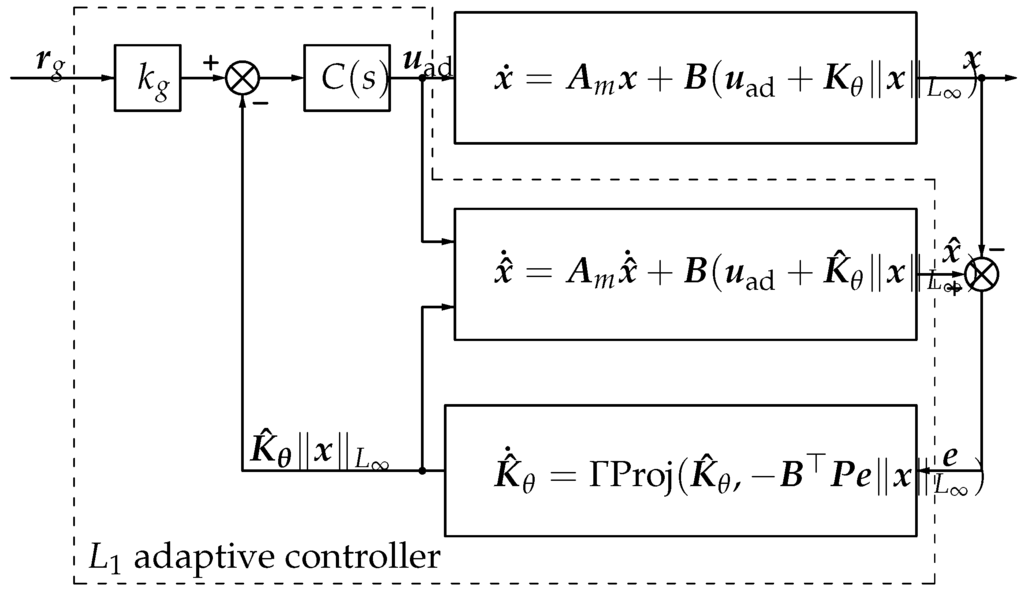
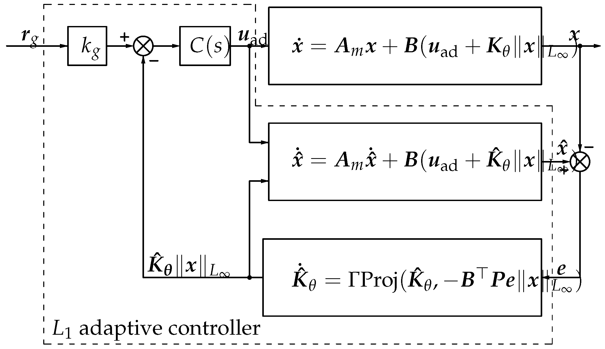
The block diagram of the adaptive control is illustrated in Figure 2.

Figure 2. $L_1$ adaptive control system algorithm.

4. Adaptive Control System Analysis

4.1. Boundedness of State Error and Parameter Error

To evaluate the performance of the adaptive control algorithm, first, we need to analyze the error boundedness. Consider the following prediction error equation derived from Equations (11) and (12):

$$\dot{\mathit{e}}(t)={\mathit{A}}_{\mathrm{m}}\mathit{e}(t)+\mathit{B}{\mathit{\theta }}_{\mathit{e}}(t)\parallel \mathit{x}(t)\parallel {}_{L_{\infty }}\mathit{e}(0)=\mathbf{0}$$

(16)

where ${\mathit{\theta }}_{\mathit{e}}(t)={\widehat{\mathit{K}}}_{\theta }(t)-{\mathit{K}}_{\theta }(t)$. For the stability of Equation (16), we have the following proposition:

Proposition 1. 

If the adaptive input ${\mathit{u}}_{\text{ad}}$ is defined as Equation (15), then we have the following result:

$${\parallel \mathit{e}\parallel }_{L_{\infty }}\le \sqrt{{\displaystyle \frac{{\theta }_m}{{\lambda }_{min}(\mathit{P})\Gamma }}}$$

(17)

where:

$${\theta }_m\triangleq 4\underset{\mathit{\vartheta }\in \Theta }{max}{\parallel \mathit{\vartheta }\parallel }^2+4{\displaystyle \frac{{\lambda }_{max}(\mathit{P})}{{\lambda }_{min}(\mathit{Q})}}\left(d_{\theta }\underset{\mathit{\vartheta }\in \Theta }{max}\parallel \mathit{\vartheta }\parallel \right)$$

Proof. 

First, we consider the following positive definite function:

$$V\left(\mathit{e}(t),{\mathit{\theta }}_{\mathit{e}}(t)\right)={\mathit{e}}^{\top }(t)\mathit{P}\mathit{e}(t)+{\displaystyle \frac{1}{\Gamma }}{\mathit{\theta }}_{\mathit{e}}^{\top }(t){\mathit{\theta }}_{\mathit{e}}(t)$$

(18)

Obviously,

$$V(\mathit{e}(0),{\mathit{\theta }}_{\mathit{e}}(0))={\displaystyle \frac{1}{\Gamma }}{\mathit{\theta }}_{\mathit{e}}^{\top }(0){\mathit{\theta }}_{\mathit{e}}(0)\le {\displaystyle \frac{1}{\Gamma }}\underset{\mathit{\vartheta }\in \Theta }{max}{\parallel \mathit{\vartheta }\parallel }^2\le {\displaystyle \frac{{\theta }_m}{\Gamma }}$$

(19)

The derivative of V about t is:

$$\begin{array}{cc}\hfill \dot{V}(\mathit{e},{\mathit{\theta }}_{\mathit{e}})=& {\dot{\mathit{e}}}^{\top }\mathit{P}\mathit{e}+{\mathit{e}}^{\top }\mathit{P}\dot{\mathit{e}}+{\displaystyle \frac{2}{\Gamma }}{\mathit{\theta }}_{\mathit{e}}{\dot{\widehat{\mathit{K}}}}_{\theta }-{\displaystyle \frac{2}{\Gamma }}{\mathit{\theta }}_{\mathit{e}}{\dot{\mathit{K}}}_{\theta }\hfill \\ \hfill =& -{\mathit{e}}^{\top }\mathit{Q}\mathit{e}+2{\mathit{\theta }}_{\mathit{e}}\left({\mathit{B}}^{\top }{\mathit{P}\mathit{e}\parallel \mathit{x}\parallel }_{L_{\infty }}+\text{Proj}({\widehat{\mathit{K}}}_{\theta },-{\mathit{B}}^{\top }{\mathit{P}\mathit{e}\parallel \mathit{x}\parallel }_{L_{\infty }})\right)\hfill \\ & -{\displaystyle \frac{2}{\Gamma }}{\mathit{\theta }}_e{\dot{\mathit{K}}}_{\theta }\hfill \end{array}$$

(20)

According to the property of the projection operator, it follows that:

$$2{\mathit{\theta }}_{\mathit{e}}\left({\mathit{B}}^{\top }{\mathit{P}\mathit{e}\parallel \mathit{x}\parallel }_{L_{\infty }}+\text{Proj}({\widehat{\mathit{K}}}_{\mathit{\theta }},-{\mathit{B}}^{\top }{\mathit{P}\mathit{e}\parallel \mathit{x}\parallel }_{L_{\infty }})\right)\le 0$$

(21)

Then, the derivative yields:

$$\dot{V}(\mathit{e},{\mathit{\theta }}_{\mathit{e}})\le -{\mathit{e}}^{\top }\mathit{Q}\mathit{e}-{\displaystyle \frac{2}{\Gamma }}{\mathit{\theta }}_{\mathit{e}}{\dot{\mathit{K}}}_{\mathit{\theta }}\le -{\mathit{e}}^{\top }\mathit{Q}\mathit{e}+{\displaystyle \frac{2}{\Gamma }}\parallel {\mathit{\theta }}_{\mathit{e}}{\dot{\mathit{K}}}_{\mathit{\theta }}\parallel$$

(22)

Given that ${\widehat{\mathit{K}}}_{\mathit{\theta }}\in \Theta$, ${\mathit{K}}_{\mathit{\theta }}\in \Theta$ and $\parallel {\dot{\mathit{K}}}_{\mathit{\theta }}\parallel \le d_{\theta }$, for any $\tau \ge 0$, the parameter error yields:

$$\begin{array}{cc}& \parallel {\mathit{\theta }}_{\mathit{e}}{\dot{\mathit{K}}}_{\mathit{\theta }}\parallel \le \parallel {\mathit{\theta }}_{\mathit{e}}\parallel ·\parallel {\dot{\mathit{K}}}_{\mathit{\theta }}\parallel =\parallel {\widehat{\mathit{K}}}_{\mathit{\theta }}-{\mathit{K}}_{\mathit{\theta }}\parallel ·\parallel {\dot{\mathit{K}}}_{\mathit{\theta }}\parallel \le 2\underset{\mathit{\vartheta }\in \Theta }{max}\parallel \mathit{\vartheta }\parallel ·d_{\theta }\hfill \\ & {\displaystyle \frac{1}{\Gamma }}{\mathit{\theta }}_{\mathit{e}}{(\tau )}^{\top }{\mathit{\theta }}_{\mathit{e}}(\tau )\le {\displaystyle \frac{4}{\Gamma }}\underset{\mathit{\vartheta }\in \Theta }{max}{\parallel \mathit{\vartheta }\parallel }^2\hfill \end{array}$$

(23)

Therefore, if, for any τ, there exists $V(\tau )>{\theta }_m/\Gamma$, the quadratic form of the prediction error has to yield:

$${\mathit{e}}^{\top }(\tau )\mathit{P}\mathit{e}(\tau )>4{\displaystyle \frac{{\lambda }_{max}(\mathit{P})}{\Gamma {\lambda }_{min}(\mathit{Q})}}\underset{\mathit{\vartheta }\in \Theta }{max}\parallel \mathit{\vartheta }\parallel d_{\theta }$$

(24)

Hence:

$${\mathit{e}}^{\top }(\tau )\mathit{Q}\mathit{e}(\tau )\ge {\displaystyle \frac{{\lambda }_{min}(\mathit{Q}){\mathit{e}}^{\top }(\tau )\mathit{Q}\mathit{e}(\tau )}{{\lambda }_{max}(\mathit{P})}}>{\displaystyle \frac{4}{\Gamma }}\underset{\mathit{\vartheta }\in \Theta }{max}\parallel \mathit{\vartheta }\parallel$$

(25)

which means that, for any $\tau >0$, as long as $V(\tau )>{\theta }_m/\Gamma$, its derivative yields.

$$\dot{V}(t,\mathit{x}(t))\le 0$$

(26)

Given that $V(t,\mathbf{0})\le {\theta }_m/\Gamma$, therefore, for all $t\ge 0$, it follows that:

$$V(t,\mathit{x}(t))\le {\displaystyle \frac{{\theta }_m}{\Gamma }}$$

(27)

Meanwhile, as ${\lambda }_{min}(\mathit{P}){\parallel \mathit{e}(t)\parallel }_{L_{\infty }}^2\le {\mathit{e}}^{\top }(t)\mathit{P}\mathit{e}(t)\le V(t)$, it follows that:

$${\parallel \mathit{e}(t)\parallel }_{L_{\infty }}^2\le {\displaystyle \frac{{\theta }_m}{{\lambda }_{min}(\mathit{P})\Gamma }},\forall t\ge 0$$

(28)

Then Equation (17) is proved. ☐

According to Equation (18), the parameter error yields:

$${\displaystyle \frac{1}{\Gamma }}{\mathit{\theta }}_{\mathit{e}}^{\top }{\mathit{\theta }}_{\mathit{e}}=V-{\mathit{e}}^{\top }\mathit{P}\mathit{e}\le v\le {\displaystyle \frac{{\theta }_m}{\Gamma }}$$

(29)

which leads to:

$$\parallel {\mathit{\theta }}_{\mathit{e}}{\parallel }_{L_{\infty }}\le \sqrt{{\theta }_m}$$

(30)

Therefore, the parameter error is also bounded.

4.2. Boundedness of State Variables

To analyze the boundedness of the system state $\mathit{x}(t)$, we first consider the following ideal system:

$${\dot{\mathit{x}}}_{\text{id}}(t)={\mathit{A}}_{\mathrm{m}}{\mathit{x}}_{\text{id}}(t)+\mathit{B}\left({\mathit{K}}_{\mathit{\theta }}\parallel {\mathit{x}}_{\text{id}}(t)\parallel \infty +{\mathit{u}}_{\text{id}}(t)\right){\mathit{x}}_{\text{id}}(0)={\mathit{x}}_0$$

(31)

The ideal control signal is:

$${\mathit{u}}_{\text{id}}(s)=-C(s)\mathit{\eta }(s)$$

(32)

where $\mathit{\eta }(s)$ is the Laplace transform of $\mathit{\eta }(t)={\mathit{K}}_{\theta }(t){\parallel {\mathit{x}}_{\text{id}}(t)\parallel }_{\infty }$.

We define $G(s)\triangleq {(s{\mathbb{I}}_4-{\mathit{A}}_{\mathrm{m}})}^{-1}\mathit{B}(s{\mathbb{I}}_2-C(s))$ and $L\triangleq {max}_{\vartheta \in \Theta }{\parallel \vartheta \parallel }_1$, where ${\mathbb{I}}_4$ and ${\mathbb{I}}_2$ are, respectively, fourth-order and second-order identity matrices. According to the definition of ${\mathit{K}}_{\theta }$ in Equation (10), $\parallel {\mathit{K}}_{\mathit{\theta }}{\parallel }_{L_{\infty }}\le L$. It can be proven that ${\mathit{x}}_{\text{id}}$ in Equation (31) is banded input banded state (BIBS) stable when ${\parallel G(s)\parallel }_{L_1}L<1$.

Proof. 

According to the definition of $G(s)$, Equation (31) can be transformed to:

$$s{\mathit{x}}_{\text{id}}(s)-\mathit{x}(0)={\mathit{A}}_{\mathrm{m}}{\mathit{x}}_{\text{id}}(s)+\mathit{B}(s{\mathbb{I}}_2-C(s))\mathit{\eta }(s)$$

(33)

After performing some algebraic operations, we get:

$${\mathit{x}}_{\text{id}}(s)=G(s)\mathit{\eta }(s)+{\mathit{x}}_{\text{in}}(s)$$

(34)

where ${\mathit{x}}_{\text{in}}(s)={(s{\mathbb{I}}_4-{\mathit{A}}_{\mathrm{m}})}^{-1}{\mathit{x}}_0$. For $\forall \tau \in (0,\infty )$ and $t\in [0,\tau ]$, the following bound exists [12]:

$$\parallel {\mathit{x}}_{\text{id}\tau }{\parallel }_{L_{\infty }}\le \parallel G(s){\mathit{K}}_{\mathit{\theta }}{\parallel }_{L_1}·{∥\parallel {\mathit{x}}_{\text{id}}{(t)\parallel }_{\infty \tau }∥}_{L_{\infty }}+{\parallel {\mathit{x}}_{\text{in}\tau }\parallel }_{L_{\infty }}$$

(35)

According to the definition of the ∞-norm and the $L_1$-norm, the following bound exists:

$$\parallel {\mathit{x}}_{\text{id}\tau }{\parallel }_{L_{\infty }}\le {∥{∥{\mathit{x}}_{\text{id}\tau }(t)∥}_{\infty }∥}_{L_{\infty }}$$

(36)

Meanwhile, since $\parallel G(s){\mathit{K}}_{\mathit{\theta }}{\parallel }_{L_1}\le {\parallel G(s)\parallel }_{L_1}\parallel {\mathit{K}}_{\mathit{\theta }}{\parallel }_{\infty }\le {\parallel G(s)\parallel }_{L_1}L<1$, therefore,

$$\parallel {\mathit{x}}_{\text{id}\tau }{\parallel }_{L_{\infty }}\le {\displaystyle \frac{\parallel {\mathit{x}}_{\text{in}}{\parallel }_{L_{\infty }}}{1-\parallel G(s){\mathit{K}}_{\mathit{\theta }}{\parallel }_{L_1}}}$$

(37)

According to the definition of ${\mathit{x}}_{\text{in}}$, if it is bounded, ${\mathit{x}}_{\text{id}}$ will be bounded. Therefore, System (31) is BIBS stable.

The system in Equation (31) is equivalent to the system predictor in Equation (12) while ${\widehat{\mathit{K}}}_{\mathit{\theta }}={\mathit{K}}_{\mathit{\theta }}$. Because ${\mathit{\theta }}_{\mathit{e}}$ and ${\mathit{x}}_{\text{in}}$ are both bounded, $\widehat{\mathit{x}}$ is bounded. Meanwhile, since $\mathit{e}=\widehat{\mathit{x}}-\mathit{x}$ and $\mathit{e}$ is also bounded, therefore, $\mathit{x}$ is bounded, i.e., System (2) is BIBS stable under the $L_1$-controller. ☐

4.3. Performance of the Adaptive System

According to Equation (17), the prediction error $\mathit{e}$ can be reduced by enhancing ${\lambda }_{min}(\mathit{P})$ or the adaptive gain Γ. ${\lambda }_{min}(\mathit{P})$ depends on the performance of the linear part ${\mathit{A}}_{\mathrm{m}}$, i.e., the wider the stability margin of the linear part of the system is, the smaller will be the prediction error. Similarly, the increase of Γ will reduce the error, as well.

5. Simulation Results for the Adaptive Control System

5.1. Simulation of the Adaptive Controller

Consider the nominal mechanical parameters in Table 1.

Table 1. Rotor parameters.

Parameter	Value	Unit
Material	Iron	–
Outer diameter	150	mm
Inner diameter	142	mm
Height	150	mm
Mass	1.737	kg

According to Table 1, the nominal rotational inertias of the rotor about the two axes are: $J_{xy0}=0.01864\text{kg}·{\mathrm{m}}^2$ and $J_{z0}=0.008439\text{kg}·{\mathrm{m}}^2$. Then, the system parameters in Equation (8) are:

$$\mathit{A}=\left[\begin{array}{cccc}0& 0& 1& 0\\ 0& 0& 0& 1\\ 161.4& 0& 0& -185.1\\ 0& 161.4& 185.1& 0\end{array}\right],\mathit{B}=\left[\begin{array}{cc}0& 0\\ 0& 0\\ 56.65& 0\\ 0& 56.65\end{array}\right]$$

(38)

The control input is:

$${\mathit{u}}_{\mathrm{m}}=-{\mathit{K}}_{\mathrm{m}}\mathit{x}=\left[\begin{array}{cccc}0& 100& 7& 0\\ -100& 0& 0& 7\end{array}\right]\mathit{x}$$

(39)

Therefore,

$${\mathit{A}}_{\mathrm{m}}=\mathit{A}-\mathit{B}{\mathit{K}}_{\mathrm{m}}=\left[\begin{array}{cccc}0& 0& 1& 0\\ 0& 0& 0& 1\\ 161.4& -5665& -396.55& -185.1\\ 5665& 161.4& 185.1& -396.55\end{array}\right]$$

(40)

Let the parameter uncertainties be ${\theta }_1=0.2J_{xy0}$ and ${\theta }_1=0.2J_{z0}$, the adaptive gain be $\Gamma =20,000$ and the low-pass filter be:

$$C(s)=\left[\begin{array}{cc}{\displaystyle \frac{3{\omega }_c^{2}s+{\omega }_c^3}{{(s+{\omega }_c)}^3}}& 0\\ 0& {\displaystyle \frac{3{\omega }_c^{2}s+{\omega }_c^3}{{(s+{\omega }_c)}^3}}\end{array}\right]$$

(41)

The bandwidth of $C(s)$ will influence the stability and performance of the system. A detailed discussion of the low-pass filter $C(s)$ is in [12].

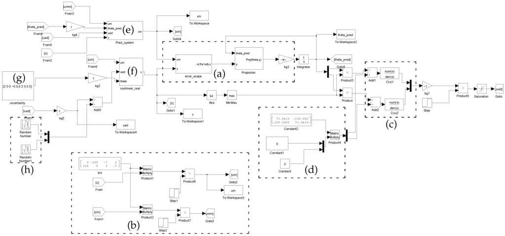
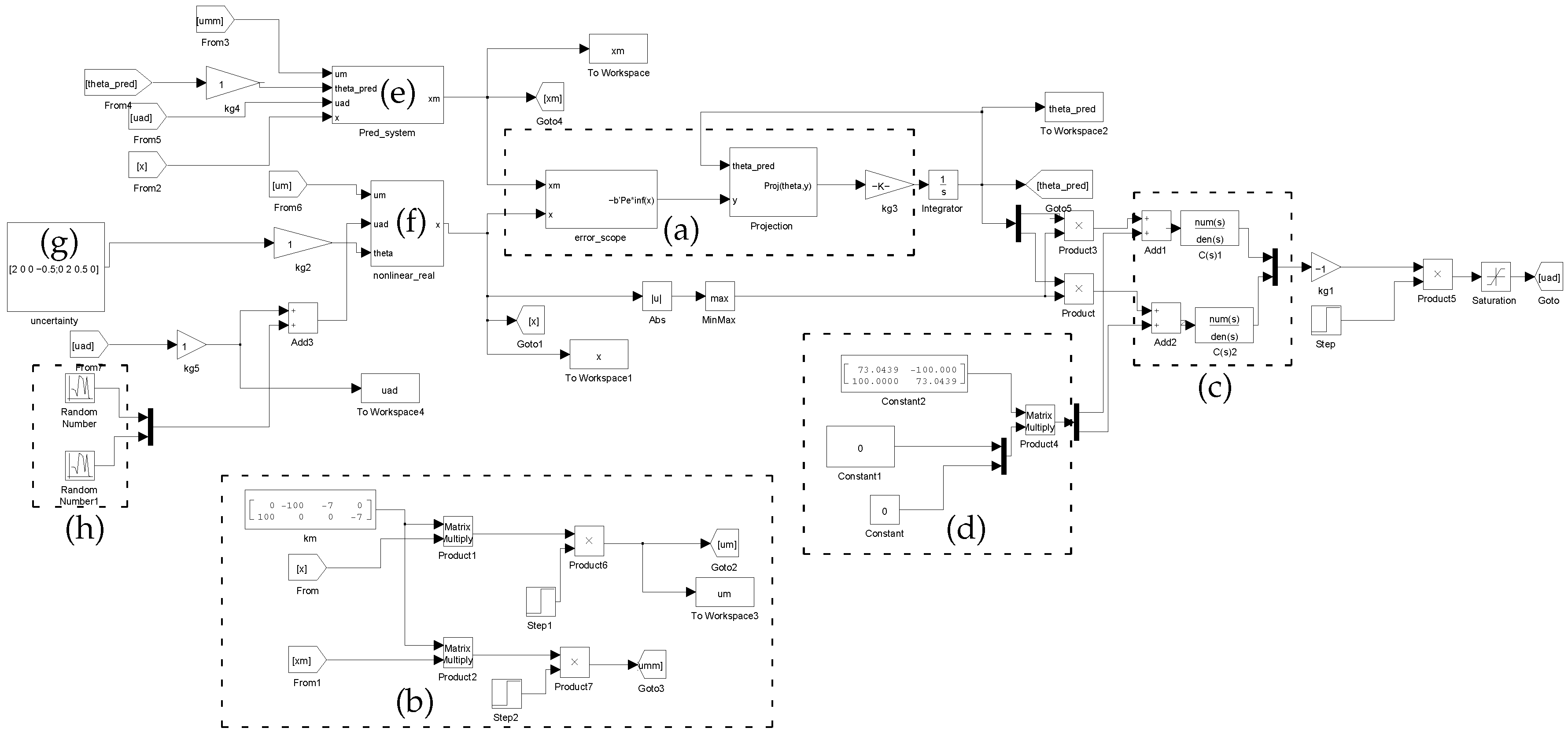
The simulation model using MATLAB/Simulink is illustrated in Figure 3. (a) is the parameter adaptive law in Equation (14); (b) is the nonadaptive control input ${\mathit{u}}_{\mathrm{m}}$ in Equation (39); (c) is the low-pass filter $C(s)$ in Equation (41); (d) is the reference input, which is zero in this paper’s situation; (e) is the state predictor in Equation (12); (f) is the plant system in Equation (2); (g) gives the parameter uncertainties; (h) is the external disturbance.

Figure 3. Block diagram in Simulink.

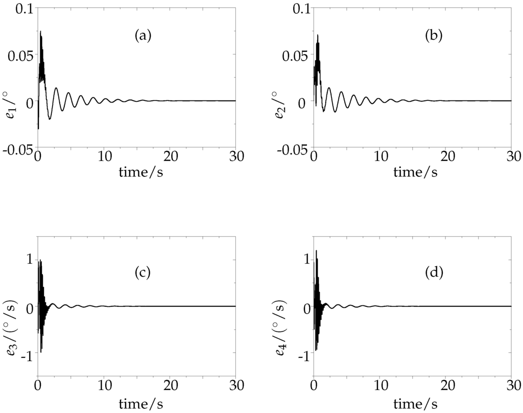
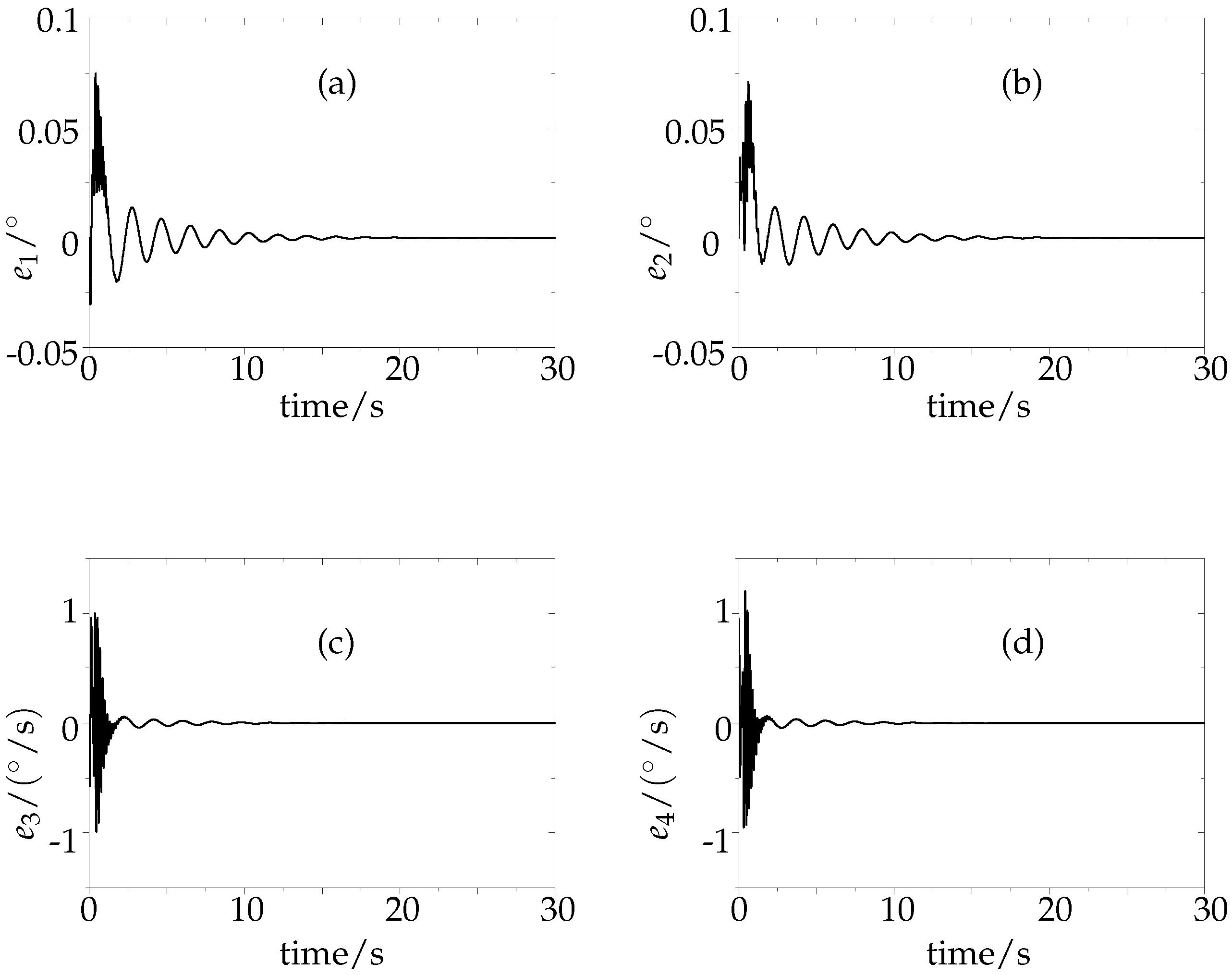
The simulation results for the prediction error in every component are shown in Figure 4. All of the components of the prediction error get reduced as time progresses.

Figure 4. Prediction error simulation results for: (a) the x-direction component $e_1$; (b) the y-direction component $e_2$; (c) the x-direction angular error $e_3$; and (d) y-direction angular error $e_4$.

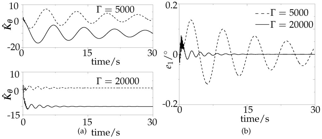
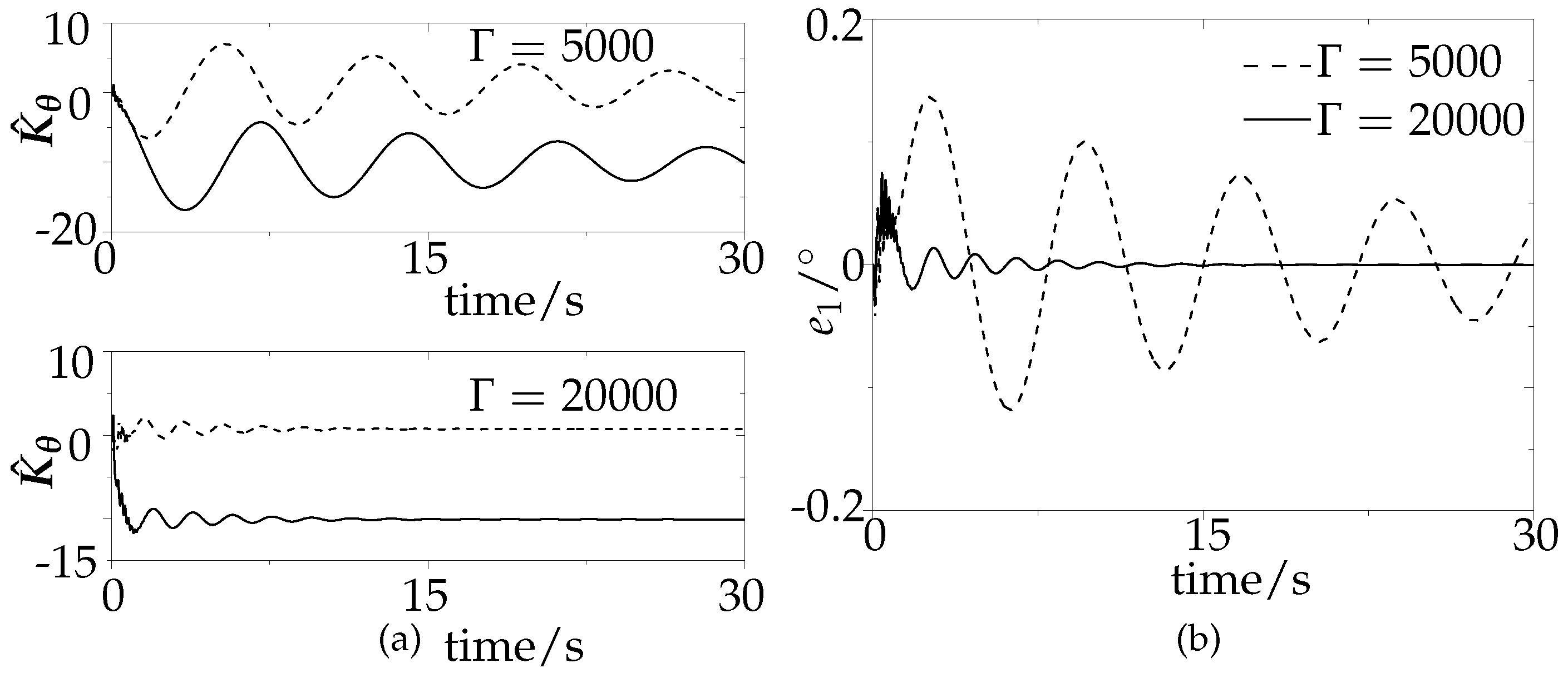
The variation trends of system parameter prediction, ${\widehat{\mathit{K}}}_{\theta }$, and one of the prediction error components, $e_1$, under different adaptive gains are shown in Figure 5. It can be seen that, when Γ is larger, ${\widehat{\mathit{K}}}_{\theta }$ and $e_1$ will converge more quickly. Therefore, Γ should be as large as possible, as long as the actuator of the control system can be achieved.

Figure 5. Simulation comparison for Γ values: (a) comparison of parameter ${\mathit{K}}_{\mathit{\theta }}$; (b) comparison of error $e_1$.

5.2. Simulation of the Rotor Orientation System

Figure 4 and Figure 5 imply that the adaptive control algorithm in Equations (14) and (15) is effective. On this basis, to further simulate the performance of the orientation system, we introduce more uncertainties. Besides the parameter uncertainty, consider the following uncertain system:

$$\dot{\mathit{x}}={\mathit{A}}_{\mathrm{m}}\mathit{x}+\mathit{B}({\mathit{u}}_{\text{ad}}+{\mathit{K}}_{\theta }{\parallel \mathit{x}\parallel }_{\infty }+\mathit{\sigma }),\mathit{x}(0)={\mathit{x}}_0$$

(42)

where $\mathit{\sigma }$ refers to an external random disturbance. Unlike Equation (11), here $\mathit{\sigma }\ne \mathbf{0}$.

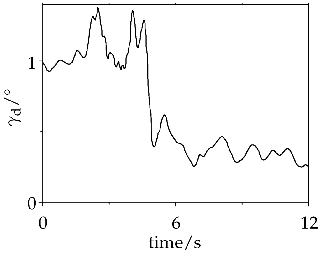
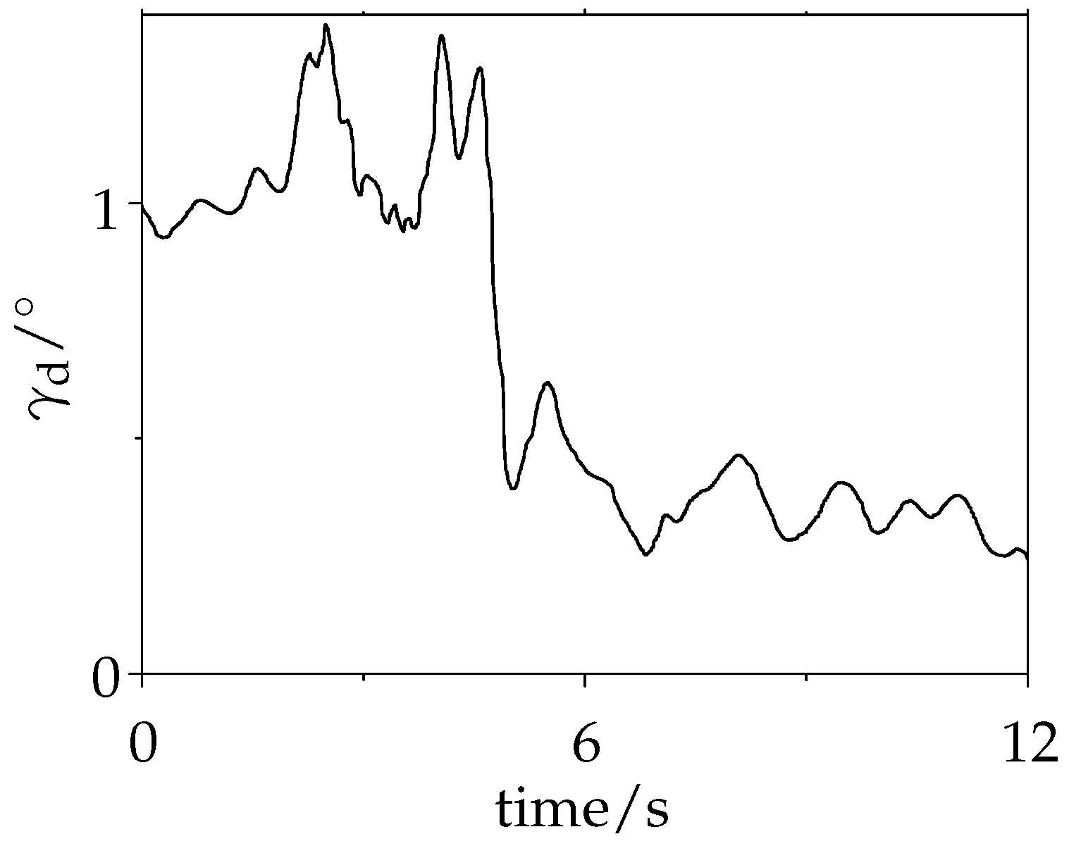
Let the adaptive controller activate at $t=4\mathrm{s}$, then we obtain the result of the rotor angular drift, ${\gamma }_{\mathrm{d}}=\sqrt{{\alpha }^2+{\beta }^2}$, from the vertical direction, as shown in Figure 6. It is obvious that, after the controller actuates, the angular displacement of the rotor reduces from more than $>1^{\circ }$ to $<0.4^{\circ }$. Therefore, the orientation control is effective.

Figure 6. Simulation result for the orientation control system.

6. Experimental Results for the Rotor Orientation System

6.1. Experimental Devices

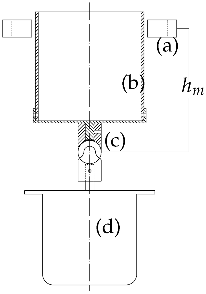
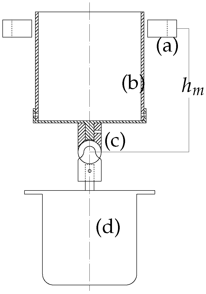
To demonstrate the feasibility of the adaptive control algorithm, we designed an experimental platform as shown in Figure 7. The iron rotor lies vertically in the center. It is connected to the drive motor at the bottom with a universal bearing, which enables the rotor to swing freely while rotating with the motor coaxially. Four electromagnets lie perpendicularly around the rotor to provide the orientation control forces. Two gap sensors are installed at a ${90}^{\circ }$ interval to detect the attitude of the rotor and provide feedback signals to the control system.

Figure 7. Experimental platform for the orientation control system: (a) electromagnet; (b) rotor; (c) universal joint; (d) motor.

6.2. Experimental Process

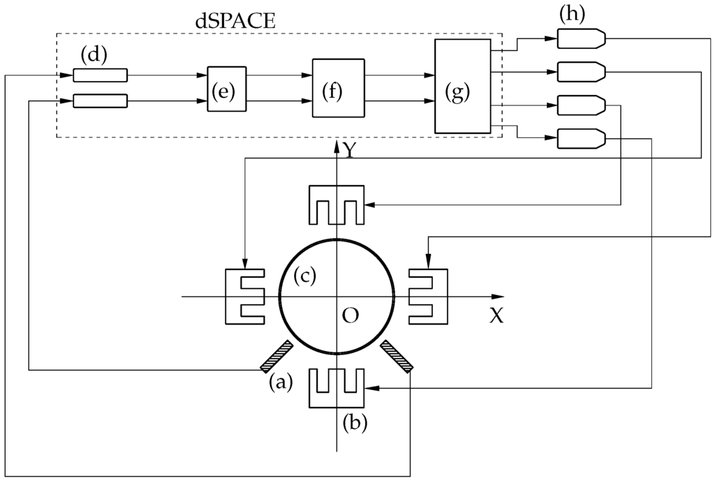
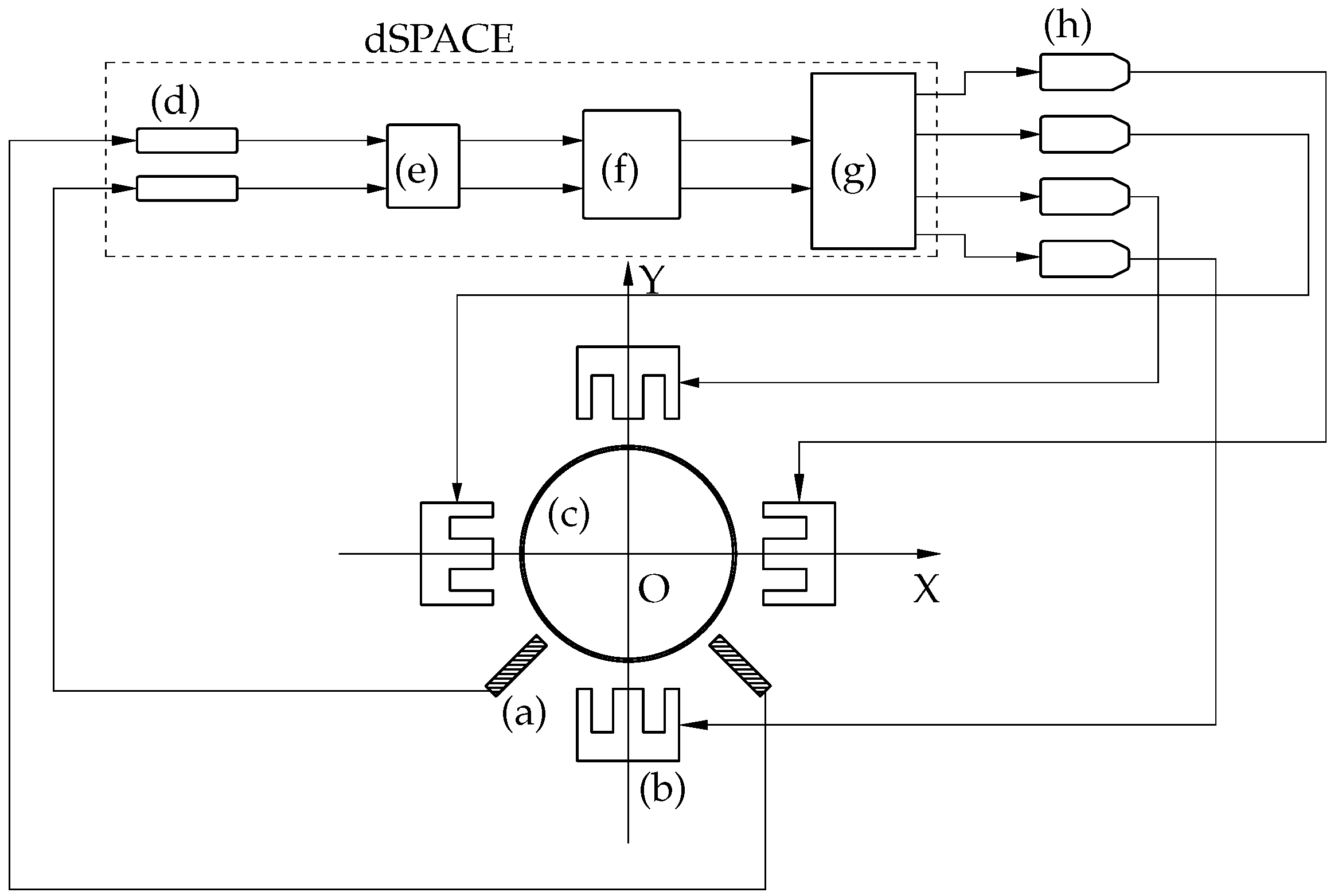
The block diagram is illustrated in Figure 8. In the experiment, we choose dSPACE as the digital controller.

Figure 8. Block diagram of the orientation experiment: (a) gap sensor; (b) electromagnet; (c) rotor; (d) gap calculation; (e) angle calculation; (f) controller; (g) control current calculation; (h) power amplifier.

The experimental program is as follows:

1.

Measurement of the rotor drift angle.

The drift angles of the rotor in the $X/Y$ directions $angl{e}_x$ and $angl{e}_y$, respectively, are converted from the two gap values $ga{p}_1$ and $ga{p}_2$. The two angles are the state variables $x_1$ and $x_2$ in Equation (2).

2.

Calculation of the electromagnetic force.

According to Equations (15) and (39), the control torque is:

$$\mathit{u}=\left[\begin{array}{c}{T}_{x\mathrm{e}}\\ T_{y\mathrm{e}}\end{array}\right]={\mathit{u}}_{\mathrm{m}}+{\mathit{u}}_{\text{ad}}$$

(43)

The torque is given by:

$$\left\{\begin{array}{cc}{T}_{x\mathrm{e}}=(F_{y-}-F_{y+})h_{\mathrm{m}}\hfill & \\ T_{y\mathrm{e}}=(F_{x+}-F_{x-})h_{\mathrm{m}}\hfill & \end{array}\right.$$

(44)

where $F_{x+},F_{x-},F_{y+}$ and $F_{y-}$ are the forces of each electromagnet in the X and Y directions and $h_{\mathrm{m}}$ is the installation height of the electromagnets.

Because the electromagnetic force can only be attractive, to make them continuous and smooth, the forces of each direction are realized via a bias control, i.e.,

$$\left\{\begin{array}{cc}\hfill F_{x+}& =F_{\mathrm{n}0}+{\displaystyle \frac{M_{y\mathrm{e}}}{2h_{\mathrm{m}}}}\hfill \\ \hfill F_{x-}& =F_{\mathrm{n}0}-{\displaystyle \frac{M_{y\mathrm{e}}}{2h_{\mathrm{m}}}}\hfill \\ \hfill F_{y+}& =F_{\mathrm{n}0}-{\displaystyle \frac{M_{x\mathrm{e}}}{2h_{\mathrm{m}}}}\hfill \\ \hfill F_{x-}& =F_{\mathrm{n}0}+{\displaystyle \frac{M_{x\mathrm{e}}}{2h_{\text{m}}}}\hfill \end{array}\right.$$

(45)

where $F_{\mathrm{n}0}$ is the reference value of each electromagnet, about which each force varies. The control force signal for each electromagnet is determined through Equations (43) and (45).

3.

Calculation of the current in every electromagnet.

The electromagnetic force of each electromagnet yields:

$$F={\displaystyle \frac{A{I}^2}{{(B+g)}^2}}$$

(46)

where A and B are factors corresponding to the electromagnet. Substituting Equations (46) into the control force Equations (45) gives the current signal of each electromagnet.

$$\left\{\begin{array}{cc}\hfill I_{x+}& =(B+g_{x+})\sqrt{\left(F_{\mathrm{n}0}+{\displaystyle \frac{M_{x\mathrm{c}}}{2h_{\mathrm{m}}}}\right)/A}\hfill \\ \hfill I_{x-}& =(B+g_{x-})\sqrt{\left(F_{\mathrm{n}0}-{\displaystyle \frac{M_{x\mathrm{c}}}{2h_{\mathrm{m}}}}\right)/A}\hfill \\ \hfill I_{y+}& =(B+g_{y+})\sqrt{\left(F_{\mathrm{n}0}+{\displaystyle \frac{M_{y\mathrm{c}}}{2h_{\mathrm{m}}}}\right)/A}\hfill \\ \hfill I_{y-}& =(B+g_{y-})\sqrt{\left(F_{\mathrm{n}0}-{\displaystyle \frac{M_{y\mathrm{c}}}{2h_{\mathrm{m}}}}\right)/A}\hfill \end{array}\right.$$

(47)

where $g_{x\pm }$ and $g_{y\pm }$ are the gaps of each electromagnet. The current signal in Equation (47) can be loaded onto each electromagnet via a power amplifier.

6.3. Experimental Results

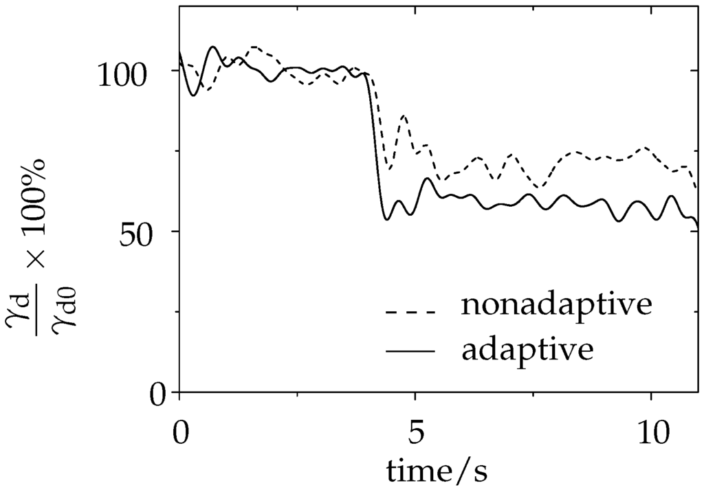
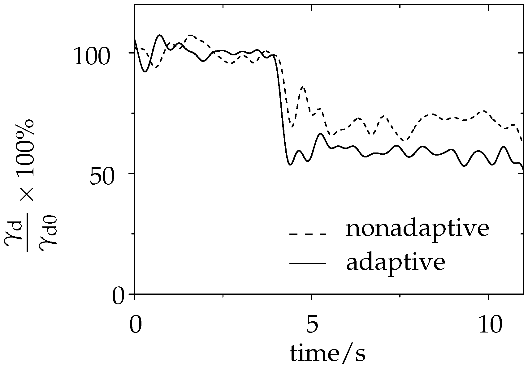
The experimental results for the orientation control system are shown in Figure 9. To clearly show the performance of the adaptive orientation control system, a result of the nonadaptive orientation control, that ${\mathit{u}}_{\text{ad}}=\mathbf{0}$ and only ${\mathit{u}}_{\mathrm{m}}$ activates, is also illustrated, as a contrast. ${\gamma }_{d0}$ is the average angular displacement without control, which is about $0.8^{\circ }$ of the adaptive control and $0.7^{\circ }$ of the nonadaptive control. The control system starts to actuate at $t=4\mathrm{s}$.

Figure 9. Experimental results for the angular drift of the rotor orientation system.

It can be seen from Figure 5 that, after the controller activates, the average angular displacement of the rotor from the vertical direction reduces to less than ∼50% of the adaptive controller and about ∼60% of the nonadaptive controller. The adaptive controller has a better performance in vibration reduction.

Furthermore, by comparing Figure 9 with Figure 6, it can be seen that the trend of the angular displacement is basically the same.

7. Conclusions

In the paper, an adaptive orientation control system for a vertical low-speed rotor is presented. The nonlinearity and parameter uncertainty are transformed into an equivalent linear time-varying form about the norm of the system state. Then, an adaptive algorithm is established based on the state predictor, and an adaptive position control method is presented to overcome the parameter uncertainty, nonlinearity and random disturbance. The stability and boundedness of the prediction error has been analyzed. The analysis indicates that the prediction error is uniformly bounded and that the bound is inversely proportional to the square root of the adaptive gain. Meanwhile, the state of the adaptive control system is BIBS stable. Finally, the control system is verified via simulation and experiment. Simulation results demonstrate the boundedness of the prediction error and the parameter estimation. The experimental result shows that the position control method reduces the amplitude of rotor vibration effectively during rotation. The work in this paper is of significance for control methods and the design of vertical AMB systems and similar rotor mechanical systems.

References

- Bae, S.; Lee, J.; Kang, Y.; Kang, J.; Yun, J. Dynamic analysis of an automatic washing machine with a hydraulic balancer. J. Sound Vib. 2002, 257, 3–18. [Google Scholar] [CrossRef]
- Chen, H.W.; Zhang, Q.J. Stability analyses of a vertical axis automatic washing machine with a hydraulic balancer. Mech. Mach. Theory 2011, 46, 910–926. [Google Scholar] [CrossRef]
- Chen, H.W.; Zhang, Q.J.; Fan, S.Y. Study on steady-state response of a vertical axis automatic washing machine with a hydraulic balancer using a new approach and a method for getting a smaller deflection angle. J. Sound Vib. 2011, 330, 2017–2030. [Google Scholar] [CrossRef]
- Smith, R.D.; Weldon, W.F. Nonlinear control of a rigid rotor magnetic bearing system: Modeling and simulation with full state feedback. IEEE Trans. Magn. 1995, 31, 973–980. [Google Scholar] [CrossRef]
- Ahrens, M.; KuCera, L.; Larsonneur, R. Performance of a Magnetically Suspended Flywheel Energy Storage Device. IEEE Trans. Control Syst. Technol. 1996, 4, 494–502. [Google Scholar] [CrossRef]
- Lum, K.Y.; Coppola, V.; Bernstein, D. Adaptive autocentering control for an active magnetic bearing supporting a rotor with unknown mass imbalance. IEEE Trans. Control Syst. Technol. 1996, 4, 587–597. [Google Scholar]
- Gibson, N.S.; Choi, H.; Buckner, G.D. H control of active magnetic bearings using artificial neural network identification of uncertainty. In Proceedings of the IEEE International Conference on Systems, Man and Cybernetics, Washington, DC, USA, 5–8 October 2003; Volume 2, pp. 1449–1456.
- Sivrioglu, S. Adaptive backstepping for switching control active magnetic bearing system with vibrating base. Control Theory Appl. IET 2007, 1, 1054–1059. [Google Scholar] [CrossRef]
- Mushi, S.E.; Lin, Z.; Allaire, P.E. Design, construction, and modeling of a flexible rotor active magnetic bearing test rig. IEEE/ASME Trans. Mechatron. 2012, 17, 1170–1182. [Google Scholar] [CrossRef]
- Tsai, N.; Kuo, C.; Lee, R. Regulation on radial position deviation for vertical AMB systems. Mech. Syst. Signal Process. 2007, 21, 2777–2793. [Google Scholar] [CrossRef]
- Shi, M.; Wang, D.; Zhang, J. Nonlinear dynamic analysis of a vertical rotor-bearing system. J. Mech. Sci. Technol. 2013, 27, 9–19. [Google Scholar] [CrossRef]
- Hovakimyan, N.; Cao, C. L1 Adaptive Control Theory: Guaranteed Robustness with Fast Adaptation; Society for Industrial and Applied Mathematics: Philadelphia, PA, USA, 2010; Volume 21. [Google Scholar]
- Sun, H.; Li, Z.; Hovakimyan, N.; Başsar, T.; Downton, G. L1 Adaptive Control for Directional Drilling Systems. IFAC Proc. Vol. 2012, 45, 72–77. [Google Scholar] [CrossRef]
- Nguyen, K.D.; Dankowicz, H. Adaptive control of underactuated robots with unmodeled dynamics. Robot. Auton. Syst. 2014, 64, 84–99. [Google Scholar] [CrossRef]
- Tao, C.W.; Taur, J.S.; Chang, Y.H.; Chang, C.W. A novel fuzzy-sliding and fuzzy-integral-sliding controller for the twin-rotor multi-input–multi-output system. IEEE Trans. Fuzzy Syst. 2010, 18, 893–905. [Google Scholar] [CrossRef]
- Allouani, F.; Boukhetala, D.; Boudjema, F. Particle swarm optimization based fuzzy sliding mode controller for the twin rotor MIMO system. In Proceedings of the 2012 16th IEEE Mediterranean Electrotechnical Conference, Hammamet, Tunisia, 25–28 March 2012; pp. 1063–1066.
- Nejjari, F.; Rotondo, D.; Puig, V.; Innocenti, M. Quasi-LPV modelling and non-linear identification of a twin rotor system. In Proceedings of the 2012 20th Mediterranean Conference on Control & Automation (MED), Barcelona, Spain, 3–6 July 2012; pp. 229–234.
- Rădac, M.B.; Precup, R.E.; Petriu, E.M.; Preitl, S. Iterative data-driven tuning of controllers for nonlinear systems with constraints. IEEE Trans. Ind. Electron. 2014, 61, 6360–6368. [Google Scholar] [CrossRef]
© 2016 by the authors; licensee MDPI, Basel, Switzerland. This article is an open access article distributed under the terms and conditions of the Creative Commons Attribution (CC-BY) license (http://creativecommons.org/licenses/by/4.0/).