Automatic Calibration Strategy Based on Artificial Neural Networks for Shift Control of Automatic Transmission

Abstract

As the number of gears in automatic transmissions (AT) increases, the calibration parameters in the gear shift control process of the transmission control unit (TCU) increase exponentially, significantly increasing the calibration workload during engineering development. To address the challenges of high cost and long cycle times associated with traditional manual calibration, this paper proposes an automatic calibration strategy for shift control based on artificial neural networks (ANNs). The core of this method lies in utilizing an ANN to establish a non-linear mapping relationship between shift characteristics and calibration parameters, thereby simulating and replacing the analysis and adjustment process of engineers. In this research, a vehicle simulation model based on a 9-speed automatic transmission (9AT) was first constructed. A large-scale dataset of shift characteristics was obtained by traversing various parameter combinations, and key features were extracted for model training. Simulation results demonstrate that the trained ANN model performs excellently in the automatic calibration process, requiring only 4 to 5 iterations to adjust shift quality to a level comparable to manual calibration. Its convergence speed and efficiency are significantly superior to traditional rule-based calibration methods. Furthermore, the model exhibits a certain degree of generalization ability and robustness across different throttle openings and gear-shifting conditions. The proposed automatic calibration method does not rely on high-precision physical models, effectively shortening the development cycle and improving calibration efficiency, which holds significant application value in the field of automatic transmission engineering development.

1. Introduction

With increasingly stringent global regulations on emissions and fuel economy, modern AT are rapidly evolving toward higher gear counts, with 10-speed variants now in series production [1]. This trend has led to an exponential increase in the complexity of control logic and the volume of associated software data. Calibration engineers are tasked with the challenge of finding a global optimal balance between three conflicting objectives across thousands of shifting patterns: shift duration, shift comfort, and clutch thermal loss [2].

The core complexity of the gearshift calibration problem stems from the system’s high degree of nonlinearity and limited observability. A typical production 10-speed transmission requires the calibration of over 22,000 labels [1,3]. Furthermore, the shifting process involves complex electromagnetic hydraulic responses, clutch engagement dynamics, and nonlinear friction characteristics that are highly sensitive to oil temperature fluctuations and component aging [4]. In industrial practice, production vehicles are typically equipped only with angular speed sensors, lacking low-cost sensors for direct measurement of hydraulic pressure or output shaft torque [5,6]. Consequently, control logic faces “blind” periods during critical stages like the fill phase and torque phase, necessitating a heavy reliance on the robustness of open-loop feedforward control [7]. Traditional manual calibration thus depends on engineers performing exhaustive road tests on prototype vehicles, which is time-consuming (often 1–2 years), costly, and prone to poor reproducibility due to uncontrollable environmental factors like traffic and weather [8,9].

To optimize shift quality and enhance calibration efficiency, various strategies have been explored. Design of Experiments (DoE) methodologies [2,8,9,10] are widely studied and involve performing extensive shifting tests on dynamometers to find optimal parameter sets offline based on objective ratings. While DoE can calibrate steady-state operations, transient conditions still require real-world tuning. Fundamentally, DoE follows a “traverse-then-optimize” logic; as gear numbers increase, the required test points grow exponentially, resulting in extremely low data efficiency. Calibrating a single legal gearshift using such black-box approaches often necessitates executing over 1500 cycles [3].

Numerous studies have applied modern control theory utilizing physical models and optimization algorithms to calculate optimal control trajectories online or offline. These include the use of Kalman Filters (KFs) [11,12,13,14,15], sliding mode observers (SMO) [16,17,18], and Luenberger observers for driveline torque estimation [13,17,19]; pseudo-spectral methods for optimal trajectory planning [20,21,22,23]; a sliding mode controller (SMC) is used to precisely track the optimized target oil pressure [24,25]; and model predictive control (MPC) for real-time coordination of clutch and engine torques [26,27,28]. Variants like integrated MPC (i-MPC) can anticipate transitions between the torque and inertia phases for smoother shifts [29], while linear quadratic regulators (LQR) are used to balance jerk and friction work in multi-objective functions [12,16,27,30]. However, these strategies rely heavily on high-fidelity models. Physical models often fail to capture the full transient characteristics of hydraulic systems and are highly sensitive to modeling errors, hydraulic delays, and lags, which often lead to closed-loop control inaccuracies.

Beyond these approaches, some researchers have utilized data-driven predictive control to plan optimal trajectories online [22,31]. Iterative learning control (ILC) has been proposed for the offline calibration and iterative update of fill phase parameters, often converging in 2–3 iterations [32], and has been extended to the torque and inertia phases [3,33,34]. With the rise in artificial intelligence, scholars have applied reinforcement learning (RL) to achieve parameter adaptation with a small number of trials [23,35]. Others have utilized gated recurrent units (GRUs) to plan clutch target positions and trajectories in real-time. However, these advanced strategies often impose a high computational burden, making them difficult to integrate directly into resource-constrained vehicle controllers.

In summary, with the exception of DoE, most existing research follows a logic chain of: establishing high-fidelity models, estimating intermediate variables, planning optimal trajectories, observing shift characteristics, and optimizing control parameters. This leads to high model dependence, complex control logic, significant closed-loop latency, and heavy computational loads, which restrict practical application. In contrast, a human engineer optimizes specific control parameters directly based on observed shift characteristics [32]. If artificial intelligence (AI) could directly learn this calibration experience to establish a nonlinear mapping between shift features and control parameters, the complex modeling and planning stages could be bypassed. Given that shift characteristics are physically similar across all AT systems, a trained AI model could theoretically adapt to various operating conditions and different transmissions.

Therefore, to validate the feasibility of this research approach, this study trains a neural network model offline using a large amount of shift data specifically for the most critical base pressure among the manually calibrated parameters, directly establishing a nonlinear mapping between shift characteristics and the base pressure parameter, and invokes this neural network model online to adjust the base pressure parameter. The remainder of this paper is organized as follows: Section 2 presents the physical model used for simulation and defines the shift control strategy, analyzing the relationship between features and parameters. Section 3 introduces the automated calibration strategy based on human-expert rules and the neural network training process. Section 4 provides simulation validation, and Section 5 offers conclusions.

2. Model and Gear Shift Strategy

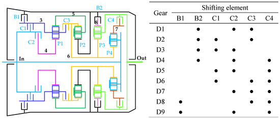
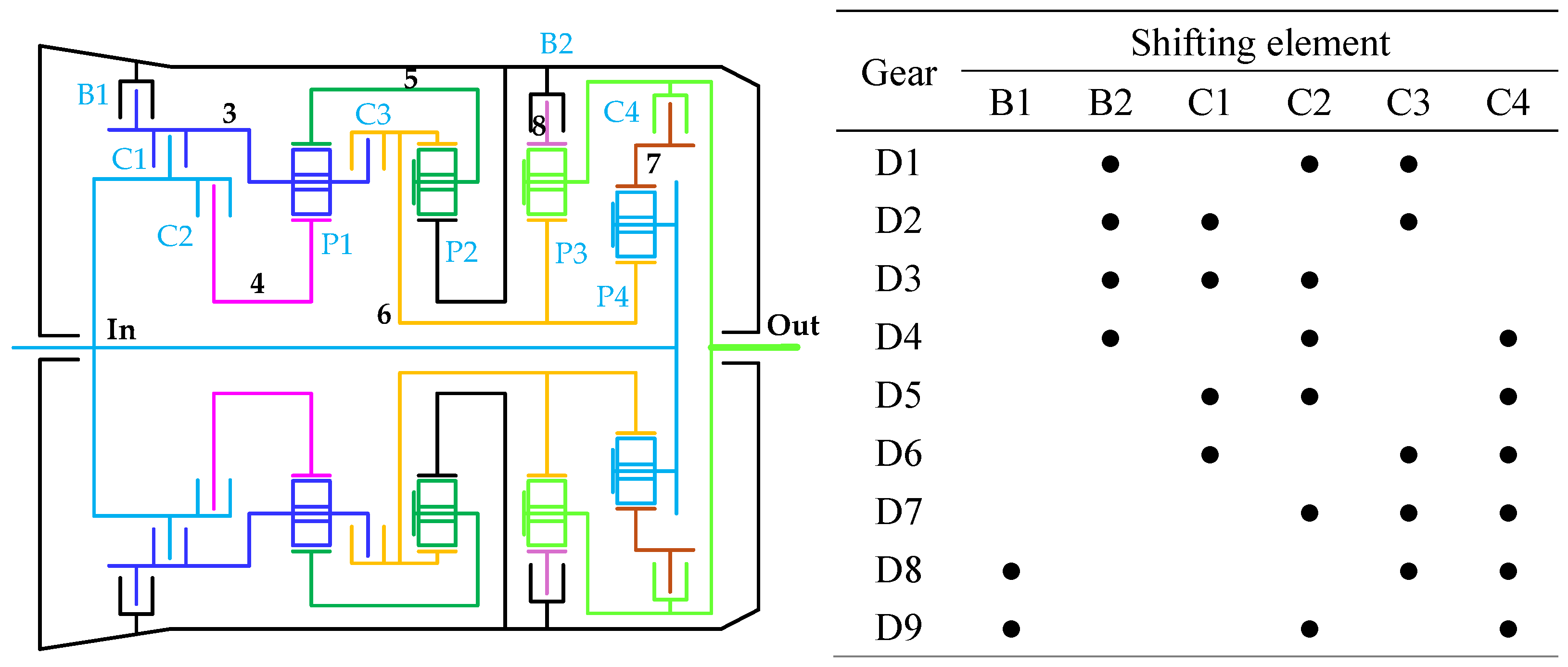
The simplified structural diagram of the transmission model is shown in Figure 1, consisting of multiple drive shafts, four sets of planetary gears, and six clutches. Calibration parameters for the oil-filling stage can be obtained through bench testing [36].

Figure 1. Scheme and shift logic of the 9AT. (Numbers 3–8 indicate the serial numbers of the shafts).

The objective of this study is to directly establish the mapping relationship between shift characteristics and calibration parameters; therefore, the overall precision of the model is not a primary concern—accurately reflecting the AT shift characteristics is sufficient to meet the research requirements of this thesis. Accordingly, the torque converter, clutch model, and the hydraulic oil filling model have been simplified or omitted, and these choices are explained in the corresponding sections. Additionally, the influence of the transmission oil temperature on the shift process is temporarily disregarded in simulations. Based on the interconnections of the transmission components, each drive shaft is modeled using Newton’s second law, with planetary gear sets linked via six clutches. The shift logic diagram is shown in Figure 1.

The following will model the clutch, shafts, and planetary gear (PG) assembly within the transmission.

2.1. Engine Model

The model of the engine is based on experimental data that maps the engine torque to the engine speed and throttle opening.

$$T_e=f({\omega }_e,P_{Th})$$

(1)

where $T_e$ and ${\omega }_e$ are the engine torque and engine speed, respectively, and $P_{Th}$ is the throttle opening.

The engine rotational dynamics are modeled by the following state equation:

$$I_{ei}{\dot{\omega }}_e=T_e-{∆T}_{ec}-T_i$$

(2)

where $I_{ei}$ is the lumped moment of inertia of the engine and the torque converter impeller, $T_i$ is the impeller torque, and ${∆T}_{ec}$ is the engine torque reduction amount implemented through ignition timing delay or fuel cut action to improve the shift quality [37]. The lower and upper limits of engine torque reduction ${∆T}_{ec}$ are set to 0 (no cut) and $T_e$ (full cut), respectively.

2.2. Torque Converter Model

The torque converter is modeled by nonlinear static maps describing dependencies of the torque ratio $R_{Tq}$ and the capacity factor $K_i$ on the turbine-impeller speed ratio $R_{\omega }={\omega }_{in}/{\omega }_e$ [38]:

$$T_i={\displaystyle \frac{{\omega }_e^2}{K_i^2\left(R_{\omega }\right)}}$$

(3)

$$T_{in}=R_{Tq}\left(R_{\omega }\right)T_i$$

(4)

where $T_{in}$ is the turbine torque.

2.3. Clutch Model

Because the clutch friction static curve exhibits significant nonlinearity/discontinuity in the zero slip speed (static friction) region, it is difficult to apply in automatic transmission shift control optimization [39]. Multiple clutch modeling approaches were studied and compared [20]. Since this study concerns only TP and IP related to base pressure parameters and does not address the zero-slip transition phase at the end of IP, this paper adopts the simplified clutch friction model like [34,37,40]. That model simplifies behavior near zero slip speed to achieve a smooth transition at the end of IP.

In this paper, the clutch employs a tangent function model [37]. Under specified pressure and slip conditions, the torque transmitted by the clutch is expressed as follows:

$$T_C=\mu ·n·r·\left(A·p-F_S\right)\tanh \left(∆\omega /a\right)$$

(5)

$$T_C=T_{\mathit{Cap}}·\tanh \left(∆\omega /a\right)$$

(6)

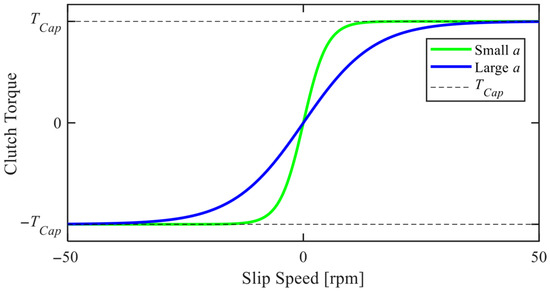
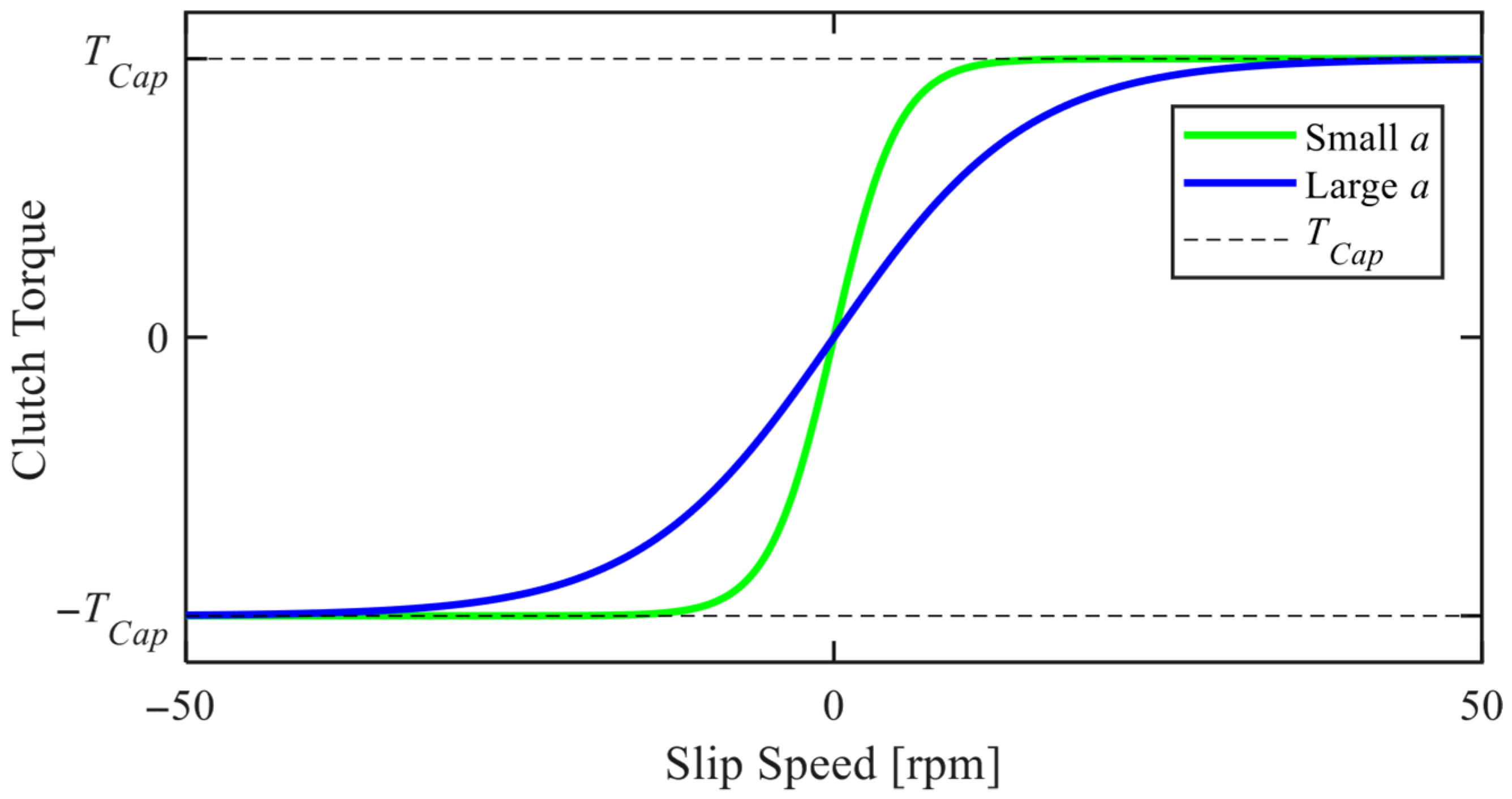
$T_C$ denotes the torque transmitted by the clutch, $\mu$ represents the clutch friction coefficient, $n$ indicates the number of friction surfaces, $r$ signifies the equivalent radius, $A$ denotes the clutch friction area, $p$ represents the clutch pressure, and $F_S$ indicates the return spring force, $∆\omega$ denotes clutch slip, $T_{Cap}$ represents clutch torque capacity, and $a$ indicates the slip coefficient. The influence of $a$ is illustrated in Figure 2. This means that at the end of IP (when the clutch locks up), slip cannot be eliminated. When $a$ is large, the slip at clutch closure is greater, but this also implies a smoother closure process. However, this study does not address the effects of that phase [37].

Figure 2. The mathematical model of clutch reverse cutting with different $a$.

2.4. Shaft Model

In other studies, the drive shaft is often modeled as a spring-damper system to achieve higher model accuracy. However, the objective of the modeling in this paper is to establish a practical simulation model without formulating state equations; therefore, the drive shaft is treated as a rigid body in this work. The dynamic model of the shaft is as follows:

$$T_{drive}-T_{React}=J·a$$

(7)

$T_{drive}$ denotes the drive-side torque, $T_{React}$ represents the load-side torque.

2.5. Planetary Gear Model

The PG consists of a sun gear, a ring gear, and a carrier. The force relationships among these components can be expressed as follows:

$$T_S+T_R+T_C=0$$

(8)

$T_R$ denotes the ring gear torque, $T_S$ denotes the sun gear torque, and $T_C$ denotes the carrier torque, with all three forces balanced.

The torque relationship between the components of the PG is as follows:

$$\left\{\begin{array}{c}{\displaystyle \frac{T_R}{T_S}}=-{\displaystyle \frac{Z_R}{Z_S}}\\ {\displaystyle \frac{T_C}{T_S}}={\displaystyle \frac{Z_R+Z_S}{Z_S}}\end{array}\right.$$

(9)

The rotational speed relationship between the components of the PG is as follows:

$${\omega }_S+{\displaystyle \frac{Z_R}{Z_S}}·{\omega }_R-\left(1+{\displaystyle \frac{Z_R}{Z_S}}\right){\omega }_C=0$$

(10)

$$i={\displaystyle \frac{Z_R}{Z_S}}$$

(11)

$${\omega }_S+{i·\omega }_R-\left(1+i\right){\omega }_C=0$$

(12)

$Z_R$ denotes the number of teeth on the ring gear, $Z_S$ denotes the number of teeth on the sun gear, ${\omega }_S$ denotes the rotational speed of the sun gear, ${\omega }_R$ denotes the rotational speed of the ring gear, and ${\omega }_C$ denotes the rotational speed of the carrier, $i$ denotes the ratio of the PG. $T_R$ and $T_C$ can be expressed as follows:

$$T_R=i·T_S$$

(13)

$$T_C=(i+1)·T_S$$

(14)

Driving resistance $T_R$ is expressed as:

$$T_R=\left({\displaystyle \frac{1}{2}}\rho A_d{C}_d{v}_{veh}^2+m_{vek}g\cos \left(\beta \right)+m_{veh}gf\right)·r_{whl}$$

(15)

where $\rho$ is the air density, $A_d$ is the vehicle frontal area, $C_d$ is the aerodynamic drag coefficient, $v_{veh}$ is the vehicle speed, $f$ is the friction coefficient, $m_{veh}$ is the vehicle mass, $\beta$ is the slope angle of the road, and $r_{whl}$ is the tire rolling radius.

$T_{out}$ is the driving resistance torque referred to the output shaft, and is expressed as:

$$T_{out}=T_R/{Ratio}_{Diff}$$

(16)

where ${Ratio}_{Diff}$ is the gear ratio from the output shaft to the wheel axle.

Since vehicle speed changes minimally during gear shifting, resistance can be treated as a constant value. By numbering each axis and analyzing the force relationships between the gears, and considering Equations (13) and (14), the dynamic equations for all drive shafts are shown in Equations (17)–(24).

$$J_{in}{\dot{\omega }}_{in}=T_{in}+T_{C1}+T_{C2}+(i_{PG4}+1){·T}_{PG4\_S}$$

(17)

$$J_{out}{\dot{\omega }}_{out}=T_{out}+T_{C4}+(i_{PG3}+1){·T}_{PG3\_S}$$

(18)

$$J_3{\dot{\omega }}_3=T_{B1}+T_{C1}+T_{C3}+(i_{PG1}+1){·T}_{PG1\_S}$$

(19)

$$J_4{\dot{\omega }}_4=T_{C2}+T_{PG1\_S}$$

(20)

$$J_5{\dot{\omega }}_5={i_{PG1}T}_{PG1\_S}+(i_{PG2}+1){·T}_{PG2\_S}$$

(21)

$$J_6{\dot{\omega }}_6=T_{C3}+{i_{PG2}T}_{PG2\_S}+T_{PG3\_S}+T_{PG4\_S}$$

(22)

$$J_7{\dot{\omega }}_7=T_{C4}+{i_{PG4}T}_{PG4\_S}$$

(23)

$$J_8{\dot{\omega }}_8=T_{B2}+{i_{PG3}T}_{PG3\_S}$$

(24)

$J_{out}$ is the sum of the vehicle’s equivalent rotational inertia referred to the output shaft and the inherent rotational inertia of the output shaft. $T_{C1}$, $T_{C2}$, $T_{C3}$, $T_{C4}$, $T_{B1}$ and $T_{B2}$ are the torques transmitted by the clutch or the brake. $T_{PG\_S}$ represent the torques of the sun gear in the planetary gear set.

From Equation (12) and the connection relationship between the shaft and the planetary gears, Equations (25)–(28) are obtained:

$${\omega }_4+{i_{PG1}·\omega }_5=\left(1+i_{PG1}\right){\omega }_3$$

(25)

$${i_{PG2}·\omega }_6=\left(1+i_{PG2}\right){\omega }_5$$

(26)

$${\omega }_6+{i_{PG3}·\omega }_8=\left(1+i_{PG3}\right){\omega }_{out}$$

(27)

$${\omega }_6+{i_{PG4}·\omega }_7=\left(1+i_{PG4}\right){\omega }_{in}$$

(28)

By assigning the unknown variables, which are speeds, internal force/torque, and output shaft torque, to the left side and the known (or assumed to be known) variables, which are torques of the input shaft, and brake, clutch, and driving resistance to the right side, a matrix format can be constituted as shown in Equation (29). Equations (30)–(33) show the details of such a matrix. The $\mathbf{M}$ is a 12 by 12 matrix, and it is invertible. Thus, it is possible to solve the unknown variables uniquely using Equation (34).

$$\mathbf{M}\mathsf{\Omega }=\mathbf{B}\mathbf{T}$$

(29)

$$\mathbf{M}=\left[\begin{array}{cccccccccccc}{J}_{in}& 0& 0& 0& 0& 0& 0& 0& 0& 0& 0& {-i}_{PG4}-1\\ 0& J_{out}& 0& 0& 0& 0& 0& 0& 0& 0& -i_{PG3}-1& 0\\ 0& 0& J_3& 0& 0& 0& 0& 0& -i_{PG1}-1& 0& 0& 0\\ 0& 0& 0& J_4& 0& 0& 0& 0& 1& 0& 0& 0\\ 0& 0& 0& 0& J_5& 0& 0& 0& -i_{PG1}& -i_{PG2}-1& 0& 0\\ 0& 0& 0& 0& 0& J_6& 0& 0& 0& -i_{PG2}& 1& 1\\ 0& 0& 0& 0& 0& 0& J_7& 0& 0& 0& 0& {-i}_{PG4}\\ 0& 0& 0& 0& 0& 0& 0& J_8& 0& 0& -i_{PG3}& 0\\ 0& 0& i_{PG1}-1& 1& i_{PG1}& 0& 0& 0& 0& 0& 0& 0\\ 0& 0& 0& 0& i_{PG2}-1& i_{PG2}& 0& 0& 0& 0& 0& 0\\ 0& i_{PG3}-1& 0& 0& 0& 1& 0& i_{PG3}& 0& 0& 0& 0\\ i_{PG4}-1& 0& 0& 0& 0& 1& i_{PG4}& 0& 0& 0& 0& 0\end{array}\right]$$

(30)

$$\mathsf{\Omega }=\left[\begin{array}{c}{\dot{\omega }}_{in}\\ {\dot{\omega }}_{out}\\ {\dot{\omega }}_3\\ {\dot{\omega }}_4\\ {\dot{\omega }}_5\\ {\dot{\omega }}_6\\ {\dot{\omega }}_7\\ {\dot{\omega }}_8\\ T_{PG1\_S}\\ T_{PG2\_S}\\ T_{PG3\_S}\\ T_{PG4\_S}\end{array}\right]$$

(31)

$$\mathbf{B}=\left[\begin{array}{cccccccc}1& 0& 1& 1& 0& 0& 0& 0\\ 0& 1& 0& 0& 0& 1& 0& 0\\ 0& 0& 1& 0& 1& 0& 1& 0\\ 0& 0& 0& 1& 0& 0& 0& 0\\ 0& 0& 0& 0& 0& 0& 0& 0\\ 0& 0& 0& 0& 1& 0& 0& 0\\ 0& 0& 0& 0& 0& 1& 0& 0\\ 0& 0& 0& 0& 0& 0& 0& 1\\ 0& 0& 0& 0& 0& 0& 0& 0\\ 0& 0& 0& 0& 0& 0& 0& 0\\ 0& 0& 0& 0& 0& 0& 0& 0\\ 0& 0& 0& 0& 0& 0& 0& 0\end{array}\right]$$

(32)

$$\mathbf{T}=\left[\begin{array}{c}{\mathit{T}}_{\mathit{i}\mathit{n}}\\ {\mathit{T}}_{\mathit{o}\mathit{u}\mathit{t}}\\ {\mathit{T}}_{\mathit{C}1}\\ {\mathit{T}}_{\mathit{C}2}\\ {\mathit{T}}_{\mathit{C}3}\\ {\mathit{T}}_{\mathit{C}4}\\ {\mathit{T}}_{\mathit{B}1}\\ {\mathit{T}}_{\mathit{B}2}\end{array}\right]$$

(33)

$$\mathsf{\Omega }={\mathbf{M}}^{-1}\mathbf{B}\mathbf{T}$$

(34)

Based on the mathematical model above, this paper establishes a mathematical simulation model in MATLAB/Simulink 2023b. The simulation step is set to 1 ms. System inputs include throttle pedal position and brake pedal position, while outputs include engine speed and torque, input shaft speed and torque, vehicle speed, gears, and other signals.

2.6. Shift Control Strategy

In the development of a new vehicle model, the calibration of the AT’s shift process is the most critical development task. AT typically consists of several PGs, with different gear sets connected by friction clutches. Different clutch combinations correspond to different gear ratios. During gear shift, changing the combination of engaged clutches alters the transmission ratio, thereby enabling gear changes. In this article, the 9-speed AT engages three clutches simultaneously across all gear positions, with two clutches remaining engaged between adjacent gears, which means that during gear changes, one clutch must disengage while another must engage. The clutch that needs to be engaged is called the On-coming (OC) clutch, while the other clutch that needs to be disengaged is called the Off-going (OG) clutch. Therefore, the gearshift process involves the torque transmitted by the input shaft being gradually transferred from the OG clutch to the OC clutch, while simultaneously synchronizing the rotational speeds at both sides of the OC clutch. Generally, the gearshift process is divided into three stages: the filling phase (FP), the torque phase (TP), and the inertia phase (IP).

2.6.1. Shift Control Progress

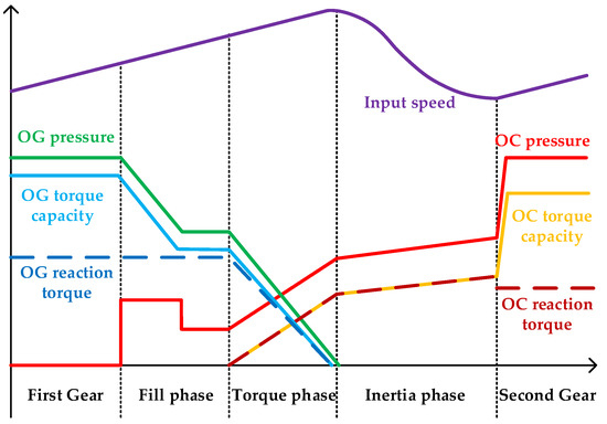
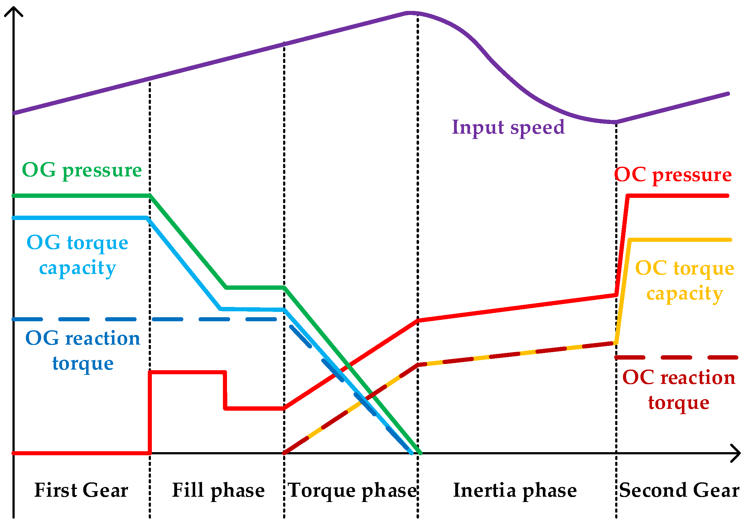
Figure 3 illustrates the changes in clutch pressure, clutch torque, and input shaft speed during the upshift from first to second gear. The clutches in AT are hydraulically driven. Therefore, before transmitting torque, the clutch must first be filled with hydraulic fluid to eliminate the air gap. This phase is called the filling phase; the OG pressure drops to the minimum pressure required to transmit the current torque. Next, the gear shift enters the torque phase, where the OC clutch and the OG clutch exchange torque. OC pressure gradually increases, progressively transmitting greater torque, while OG pressure gradually decreases to zero, with the transmitted torque gradually decreasing to zero. The torque phase would end when the torque transmitted by the transmission is fully transferred to the OC clutch. During the inertial phase, the two sides of the OC clutch are not yet synchronized. Therefore, OC pressure must be maintained or increased further until synchronization is achieved. Finally, OC pressure shall be increased to the maximum pressure to fully engage the OC clutch.

Figure 3. Power-on up gear shift progress.

During gear shift, the transmission system enters an uncontrolled state due to simultaneous changes in OC and OG pressures. Therefore, a smooth and rapid shift can only be achieved through the coordinated operation of OC and OG pressures. When the throttle changes rapidly, if control pressure varies in real time with rotational speed and torque, the actual pressure cannot promptly reach the target value. Therefore, additional compensation is required based on the gradient of torque and rotational speed [41]. Due to differing gear ratios before and after gear shift, the same input torque produces different output torques. To ensure smoothness during gear changes, torque control is also required to accelerate the synchronization process and reduce jerk [42,43,44]. The control of FP is primarily related to the physical structure of the transmission. The transmission hydraulic system is a complex nonlinear system, particularly during the oil-filling process of clutch engagement. First-principles modeling of this oil-filling process presents a challenging task, with typically higher order and only a few studies having addressed it [32,45,46,47]. Therefore, the simulation model struggles to reproduce the clutch oil filling characteristics observed in actual vehicles. In industry, standardized testing on a test bench can be conducted to obtain the FP parameters [36]. Researchers have also proposed online adaptive methods based on models and iterative learning controllers (ILC) to derive FP parameters [32,48,49]. Since the focus of this study is to explore whether ANNs can replace manual calibration rather than the specific shifting process, a simplified shifting process is adopted, and FP is not considered.

In this paper, the shift control strategy utilizes a pressure control strategy based on a fixed linear profile. To validate the automatic calibration strategy described in this paper, the shift control strategy needs to be simplified. Since the simulation model does not account for FP, this paper focuses solely on TP and IP. Furthermore, clutch pressure in the TP begins transmitting torque from zero. To simplify the number of calibration parameters, linear control is employed for pressure control during TP, while linear plus PI control is used during IP.

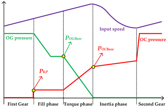
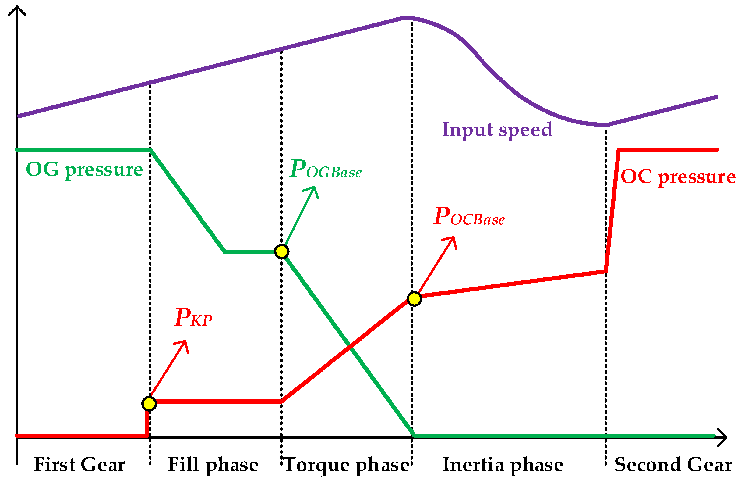
To cover the operating conditions across different rotational speeds, torques, temperatures, and gear positions, a lookup table can be used to parameterize the shift control curve. Based on calibration experience, the maximum and minimum durations of the TP and IP must be constrained. Finally, the pressure control curve trajectory of the shift clutch in this study is shown in Figure 4.

Figure 4. Shape-constrained pressure command during Power-on up gear shift.

2.6.2. Gear Shift Process Characteristic Analysis

Although the filling process of the OC clutch during FP is not considered in the simulation, the oil-draining process of the OG clutch must be taken into account. Because the OG clutch needs to reduce pressure from its maximum level to a target value that is just sufficient for the current torque transmission before TP begins.

If $P_{OCBase}$ pressure is appropriate, but $P_{OGBase}$ pressure is low, the torque capacity of the OG clutch will fall below the required transmitted torque, causing the input shaft to overspeed, which is called flare. Conversely, if $P_{OGBase}$ is too high, the torque transmitted by the OG clutch remains constant as the OG pressure decreases. Simultaneously, as OC pressure rises, the OC clutch begins to transmit torque. Both OC and OG clutch simultaneously transmitted excessive torque, causing the gear sets of both gears to be locked at the same time, which is called tie-up. As a tie-up cannot be reproduced in simulations, this study does not consider the feature.

Furthermore, if $P_{OGBase}$ is appropriate but $P_{OCBase}$ is high, the duration of TP becomes excessively short. During IP, the clutch will engage too rapidly, which induces significant fluctuations throughout the drivetrain. In contrast, if $P_{OCBase}$ is too low, when the OG pressure drops to zero, the OC pressure has not reached the required pressure that enable to transmit the full torque, which makes the input shaft flare and the duration of IP over long.

The characteristics of a flare are difficult to quantify due to the varying input speeds in different operating conditions and gears. The gear shift percentage ($GSP$) is proposed to represent the gear shift process, normalizing the input speed variation during the gear change. $GSP$ is calculated as follows:

$$GSP=(n_{TgtSlip}-n_{CurrSlip})/n_{TgtSlip}$$

(35)

$$n_{TgtSlip}=n_{InSpd}-n_{TgtSpd}$$

(36)

$$n_{CurrSlip}=n_{InSpd}-n_{CurrSpd}$$

(37)

$$n_{TgtSpd}=n_{OutSpd}·{Ratio}_{TgtGear}$$

(38)

$$n_{CurrSpd}=n_{OutSpd}·{Ratio}_{CurrGear}$$

(39)

$GSP$ represents the gear shift percentage; $n_{TgtSlip}$ represents the differ of $n_{TgtSpd}$ and $n_{InSpd}$; $n_{CurrSlip}$ represents the differ of $n_{CurrSpd}$ and $n_{InSpd}$; $n_{TgtSpd}$ represents the virtual input speed based on the target gear ratio, called the target gear speed; $n_{CurrSpd}$ represents the virtual input speed based on the current gear ratio, called the current gear speed; ${Ratio}_{TgtGear}$ represents the ratio of the target gear; ${Ratio}_{CurrGear}$ represents the ratio of the current gear.

During the gear shift process, assuming the input shaft acts as a rigid body and out shaft speed is static, dynamic equations of the input shaft throughout FP, TP, and IP can be abstractly formulated as follows:

$$J_{in}{\dot{\omega }}_{in}=T_{in}+T_{OG}$$

(40)

$$J_{in}{\dot{\omega }}_{in}=T_{in}+T_{OC}+T_{OG}$$

(41)

$$J_{in}{\dot{\omega }}_{in}=T_{in}+T_{OC}$$

(42)

Equation (40) is used in FP, Equation (41) is used in TP, and Equation (42) is used in IP.

According to Equation (5), the torque capacity of the OC and OG clutches is:

$$T_{Cap\_OC}={\mu }_{OC}·n_{OC}·r_{OC}·\left(A_{OC}·p_{OC}-F_{S\_OC}\right)$$

(43)

$$T_{Cap\_OG}={\mu }_{OG}·n_{OG}·r_{OG}·\left(A_{OG}·p_{OG}-F_{S\_OG}\right)$$

(44)

Before the inertia phase of gear shifting, to ensure smooth input shaft speed, a balance must be maintained among the three torques. During FP, the OC clutch torque is 0. In order to ensure that the input shaft does not flare, $T_{in}$ shall be less than $T_{Cap\_OG}$. The OG min pressure that can make sure $T_{in}\le T_{Cap\_OG}$, is the OG base pressure ($P_{OGBase}$). At the end of TP, the OG pressure is 0, which means the OG clutch torque is 0. In order to ensure that the input shaft does not flare, $T_{in}$ shall less than $T_{Cap\_OC}$. The OC min pressure that can make sure $T_{in}\le T_{Cap\_OC}$, is the OC base pressure ($P_{OCBase}$).

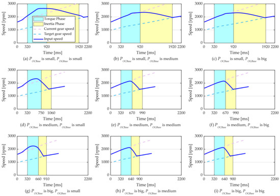
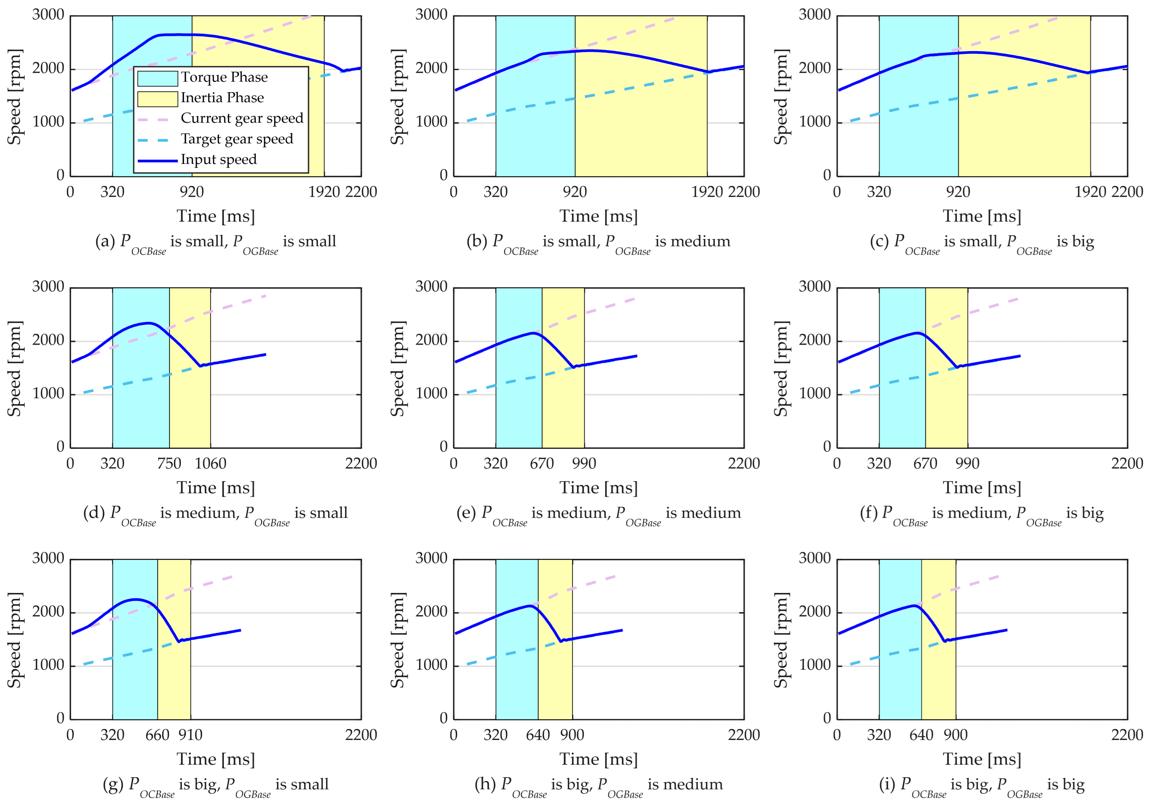
To validate the above analysis, simulations were conducted with different $P_{OCBase}$ and $P_{OGBase}$ to obtain gear-shift characteristics, as shown in Figure 5:

Figure 5. Characteristics of the gear shift process under different $P_{OCBase}$ and $P_{OGBase}$.

$GSP$ can accurately describe the variation in the input speed during the gear shift process, including the flare when $GSP$ is less than 0.

When the OG pressure is too low, the flare begins from FP, which means that the powertrain opens prematurely, and the torque that the OG clutch can transmit is less than the input torque. When OC pressure is too low, the flare begins from TP. When the OG clutch is fully disengaged, the torque capacity of the OC clutch is unable to fully handle the torque transmitted by the input shaft, which also cannot satisfy the conditions for entering the inertial stage, further resulting in excessively long durations TP and IP.

Based on the above analysis and combined with engineering practice, the following four gear shift characteristics need to be considered: flare during FP (minimum of $GSP$ during FP, ${GSP}_{Flr\_FP}$), flare during TP (minimum of $GSP$ during TP, ${GSP}_{Flr\_TP}$), duration of TP ($T_{TP}$), and duration of IP ($T_{IP}$).

During gear shift, the flare is not allowed. The durations of TP and IP do not have fixed values and are determined based on driving style and other conditions. For this article, a baseline value of 300 ms is temporarily selected, with a 50 ms margin of error added to define the allowable time range. As a result, the allowed range is determined by the following conditions:

$$\left\{\begin{array}{c}{GSP}_{Flr\_FP}=0\\ {GSP}_{Flr\_TP}=0\\ {250 \mathrm{ms}<T}_{TP}<350 \mathrm{ms}\\ {250 \mathrm{ms}<T}_{IP}<350 \mathrm{ms}\end{array}\right.$$

(45)

3. Calibration Strategy

Based on the shift process control strategy presented in this paper, the most critical work is calibrating the two parameters-$P_{OCBase}$ and $P_{OGBase}$, while the calibration method has already been described above. The automatic calibration strategy proposed integrates the mapping relationship between gear shift characteristics and calibration parameters into an ANN model. During the shift, the ANN model can analyze shift characteristics and determine the magnitudes of the calibration parameters. For comparison, a rule-based calibration strategy that is based on the calibration experience of engineers is designed.

3.1. Rule-Based Strategy

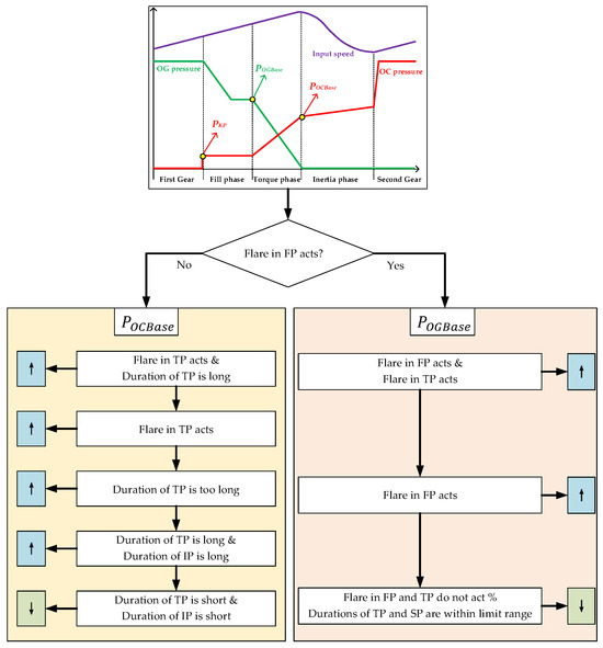
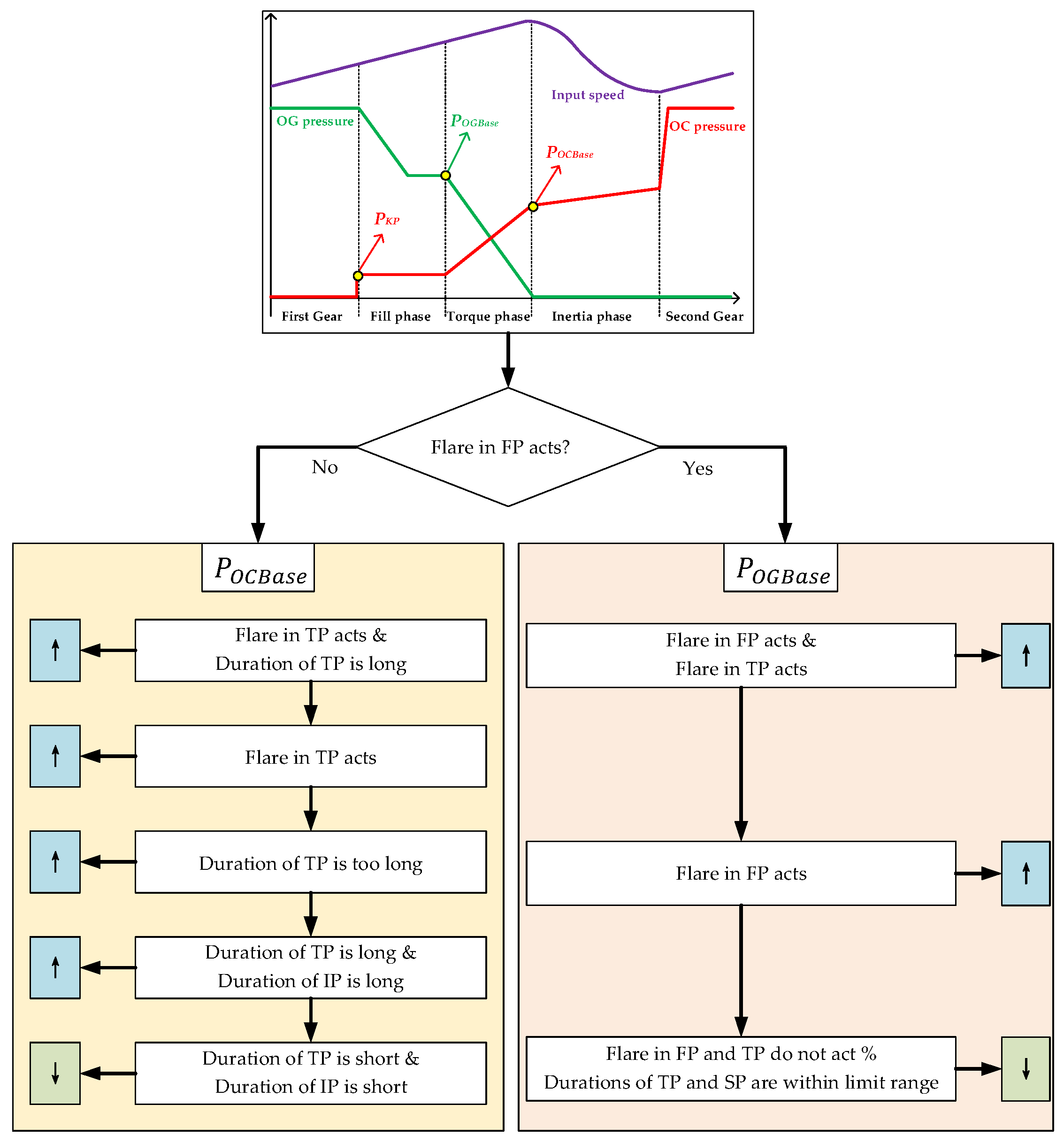
Traditional manual calibration methods rely heavily on the engineering experience, determining the pressure magnitudes of the OC and OG clutches based on features observed during the gear shift process. Drawing on engineering practical field experience, the rule-based calibration strategy designed in this paper is shown in Figure 6.

Figure 6. Automatic calibration strategy based on engineering experience rules. (An upward arrow indicates that the parameter needs to be increased, while a downward arrow indicates that the parameter needs to be decreased).

As shown in Figure 6, the rule-based strategy can only adjust one parameter at once. Flare in FP shall first be considered. If flare in FP acts, $P_{OGBase}$ shall be adjusted, while if a flare in FP does not act, $P_{OCBase}$ shall be adjusted. For $P_{OCBase}$, the engineering experience rules are as follows:

• if flare in TP actives and duration of TP is long, $P_{OCBase}$ shall increase;
• if flare in TP actives, $P_{OCBase}$ shall increase;
• if duration of TP is too long, $P_{OCBase}$ shall increase;
• if duration of TP is long and the duration of IP is long, $P_{OCBase}$ shall increase;
• if duration of TP is too short and the duration of IP is too short, $P_{OCBase}$ shall decrease.

As for $P_{OGBase}$, the engineering experience rules are as follows:

• if flare in FP actives, and flare in TP actives, $P_{OGBase}$ shall increase;
• if flare in FP actives, $P_{OGBase}$ shall increase;
• if flare in FP and TP are not active and the durations of TP and IP are within the limit range, $P_{OGBase}$ shall decrease.

The manual calibration method is essentially as described above, and will be compared with the automatic calibration method proposed in this paper.

3.2. ANN-Based Strategy

The purpose of automatic calibration is to automatically adjust the calibration parameters when driving, achieving rapid and smooth shift quality. ANNs possess strong nonlinear fitting capabilities, enabling them to emulate human analysis of complex phenomena and arrive at the most probable solution. Because ANNs resemble the human brain, they can acquire and store knowledge and experience through training. The nodes in an ANN are highly analogous to neurons in the human brain; each node represents a portion of knowledge or experience, and the interconnections among these nodes collectively form an ANN capable of learning. Like the human brain, an ANN also needs to undergo learning. Junior engineers initially require experienced engineers to teach them which features correspond to specific outcomes; through continuous learning and training, they gradually acquire extensive calibration experience. Similarly, by training an ANN with a large volume of labeled gear shift data featuring complete characteristics, an experienced ANN model can theoretically be obtained.

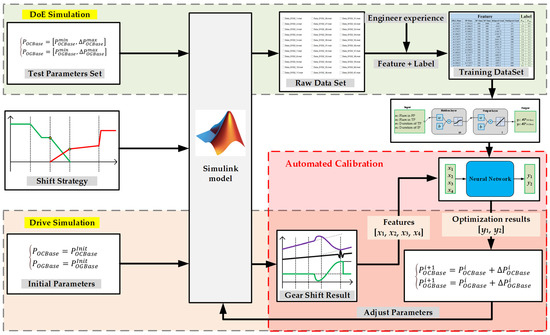
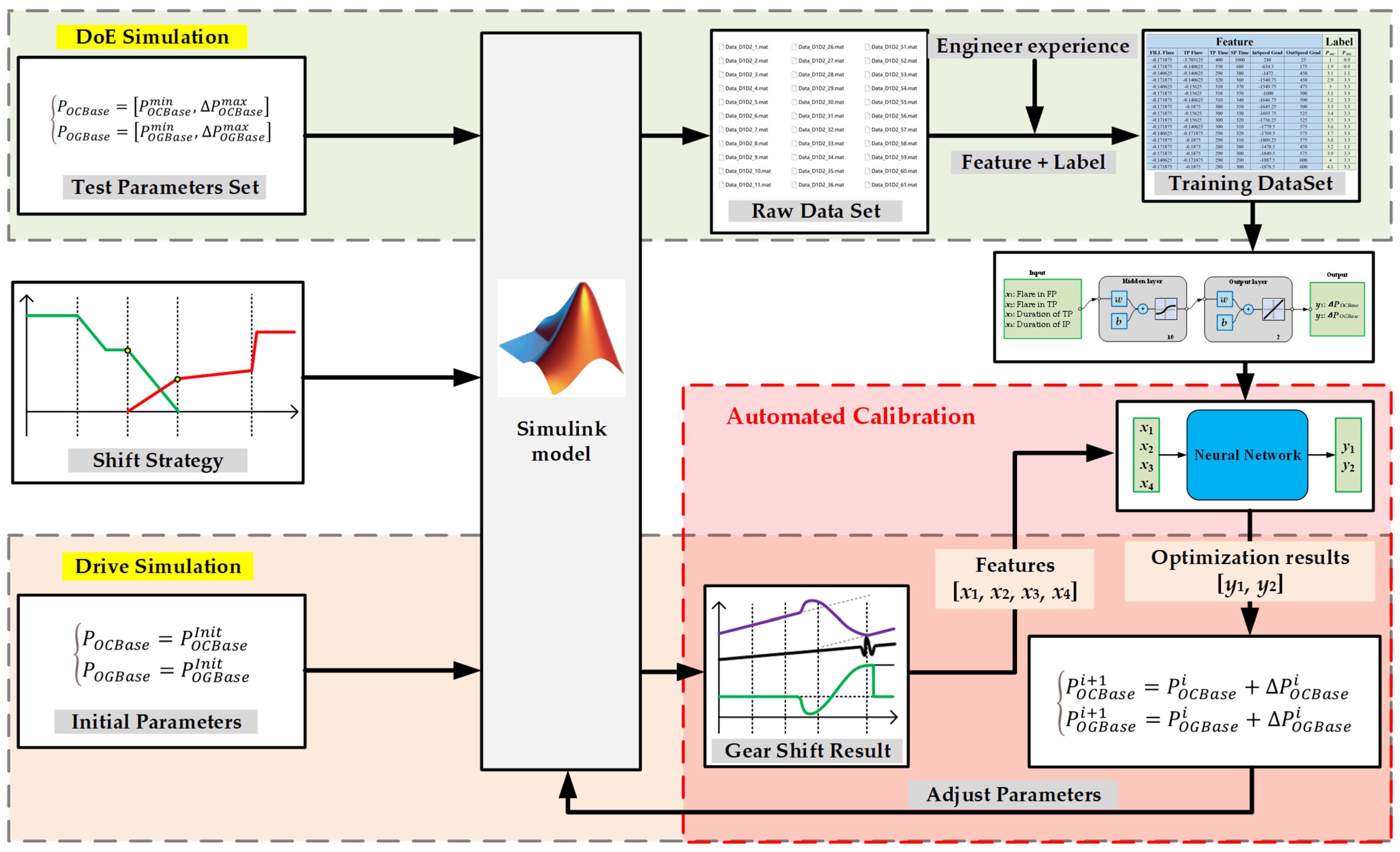
In the context of automatic calibration using the ANN fitting in the calibration process, the method proposed in this paper includes several basic steps, as shown in Figure 7. The ANN model is trained, tested, and validated in the MATLAB toolbox. First, based on the vehicle simulation model, the value ranges of the selected calibration parameters are traversed to obtain a dataset of shift results under all parameter combinations, which is then preprocessed, including normalization and data cleaning, to ensure its suitability for the ANN training. Next, an appropriate ANN architecture is selected, which needs to consider the requirements of automatic calibration, and features are extracted from the shift dataset and labeled. Finally, the processed data is input into the ANN for training to obtain an automatic calibration model that integrates the correspondence relationship between shift characteristics and calibration parameter magnitudes.

Figure 7. Schematic diagram of the automatic calibration strategy based on the ANN mode.

3.2.1. Gear Shift Data

If the ANN model is used in place of engineers to automatically adjust calibration parameters based on shift characteristics, it is first necessary to analyze whether the ANN is suitable for analyzing actual shift processes.

As mentioned above, this paper primarily studies the impact of $P_{OCBase}$ and $P_{OGBase}$ on shift quality; therefore, the training data is mainly obtained by traversing all combinations within the simulation ranges of $P_{OCBase}$ and $P_{OGBase}$.

Since clutch pressure control parameters vary under different operating conditions (such as input torque), this study conducts simulations under consistent operating conditions—specifically, gear upshift from gear 1st to gear 2nd (D1D2) with 20% throttle. The $P_{OCBase}$ parameter range is set to [3, 6] with a step of 0.05, and the $P_{OGBase}$ parameter range is set to [2.5, 5.5] with a step of 0.05, resulting in a total of 3600 parameter combinations. Finally, simulations for all combinations yield 3600 datasets. The single operating condition was chosen in this study to verify whether the ANN model is usable under that specific condition; its performance will inevitably be affected under other conditions. If the ANN model is demonstrated to be feasible, this study will attempt to address the model’s generalization capability. However, that is beyond the scope of the present work.

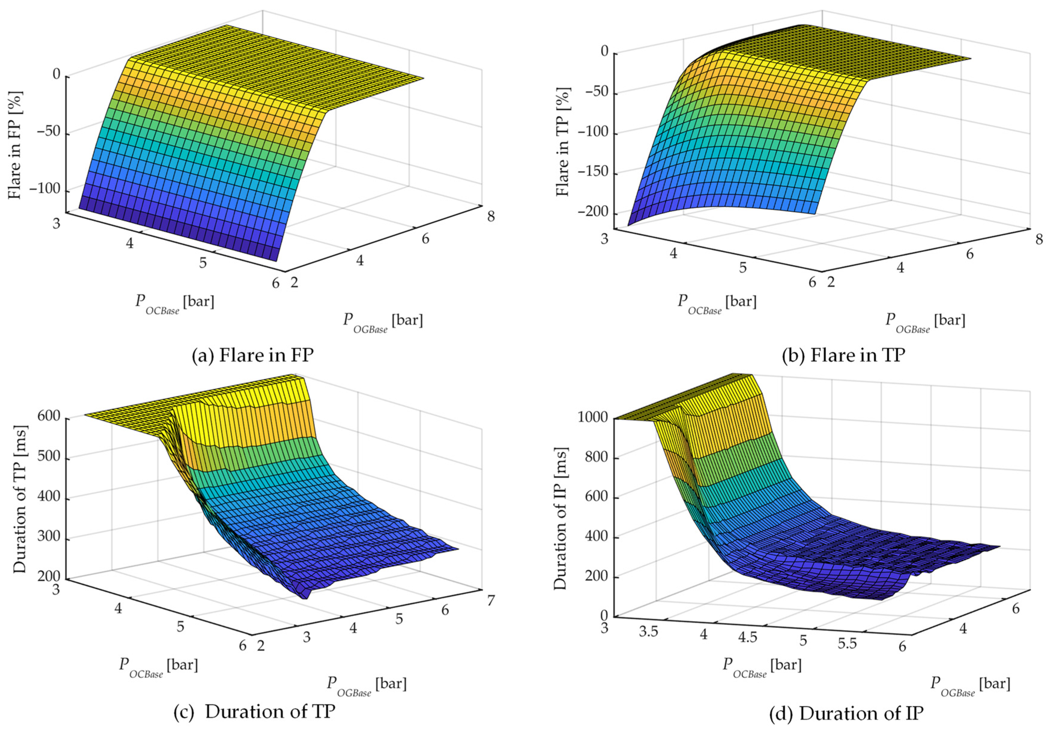
For the training data, features need to be extracted. Based on the preceding analysis, when extracting gear shift features, the following factors must be considered: flare during FP (minimum of $GSP$ during FP, ${GSP}_{Flr\_FP}$), flare during TP (minimum of $GSP$ during TP, ${GSP}_{Flr\_TP}$), duration of TP ($T_{TP}$), and duration of IP ($T_{IP}$). The distribution of gear-shift features is shown in Figure 8, revealing distinct statistical features. It is worth noting that, because the influence of FP was not taken into account, the feature set chosen in this paper aligns with the engineers’ experience. Relying on this feature set, $P_{OCBase}$ and $P_{OGBase}$ can be calibrated by the engineers.

Figure 8. Shift characteristic distribution map within the range of all parameter values.

Since the output of the ANN model during parameter calibration should indicate the degree to which the calibration parameters are large or small, the labels for the data should indicate the degree to which $P_{OCBase}$ and $P_{OGBase}$ are large or small. Therefore, the optimal values of $P_{OCBase}$ and $P_{OGBase}$ must first be determined. In this study, data that meet the target gear shift characteristic indicators described in Section 2.6.2 and Equation (45) are used as reference points. Then, the reference point ($P_{OCBase\_Ref}$ and $P_{OGBase\_Ref}$) will serve as zero points, and the difference between the parameters of other data ($P_{OCBase}$ and $P_{OGBase}$) and the optimal parameters ($P_{OCBase\_Ref}$ and $P_{OGBase\_Ref}$) will be set as the data labels.

3.2.2. Training ANN Model

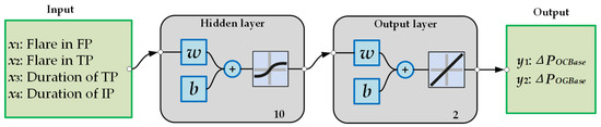
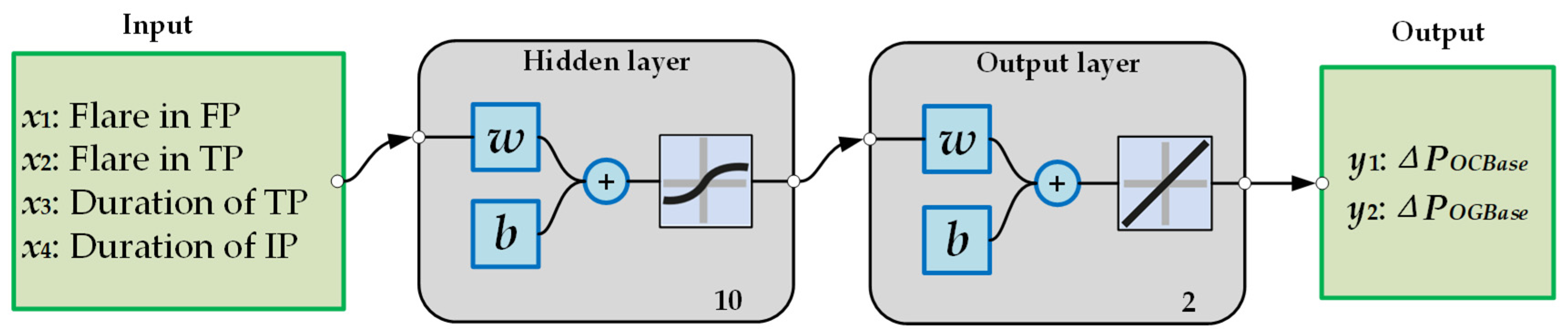
The basic structure of the ANN used in this research is shown in Figure 9.

Figure 9. The Structure of the ANN.

This is a two-layer ANN, where each neuron receives all inputs and is associated with weights and biases; after multiple layers of computation, the output is generated through an activation function. The variables of the input layer are features extracted from the gear shift process, including ${GSP}_{Flr\_FP}$, ${GSP}_{Flr\_FP}$, $T_{TP}$, and $T_{IP}$.

Considering the problem requirements and dataset characteristics, the selection of an appropriate feedforward neural network architecture is important. Several simulations were executed to assess performance across different architectural configurations, employing mean squared error (MSE) as the performance metric. The ANN model updates its weights and biases using the Levenberg–Marquardt training algorithm, which combines the advantages of the Gauss-Newton algorithm and gradient descent. It demonstrates outstanding performance across various complex fitting and optimization problems, excels at specific regression tasks, and achieves the fastest training speed. Table 1 presents the training results for the different architectures. When the number of neurons in the hidden layer exceeds 10, the MSE no longer decreases significantly. Thus, the hidden layer with 10 neurons and the output layer with 2 neurons are selected.

Table 1. Impact of Various Architectural Designs on Neural Network Performance.

Net	Layers	Number of Neurons Per Layer	MSE
Net 1	2	5, 2	0.2539
Net 2	2	10, 2	0.2209
Net 3	2	15, 2	0.2226
Net 4	2	20, 2	0.2215

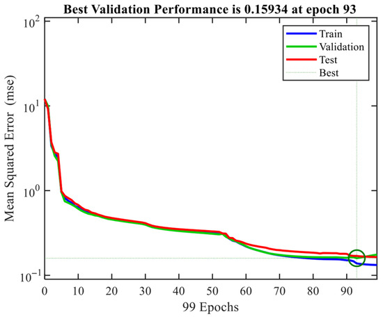
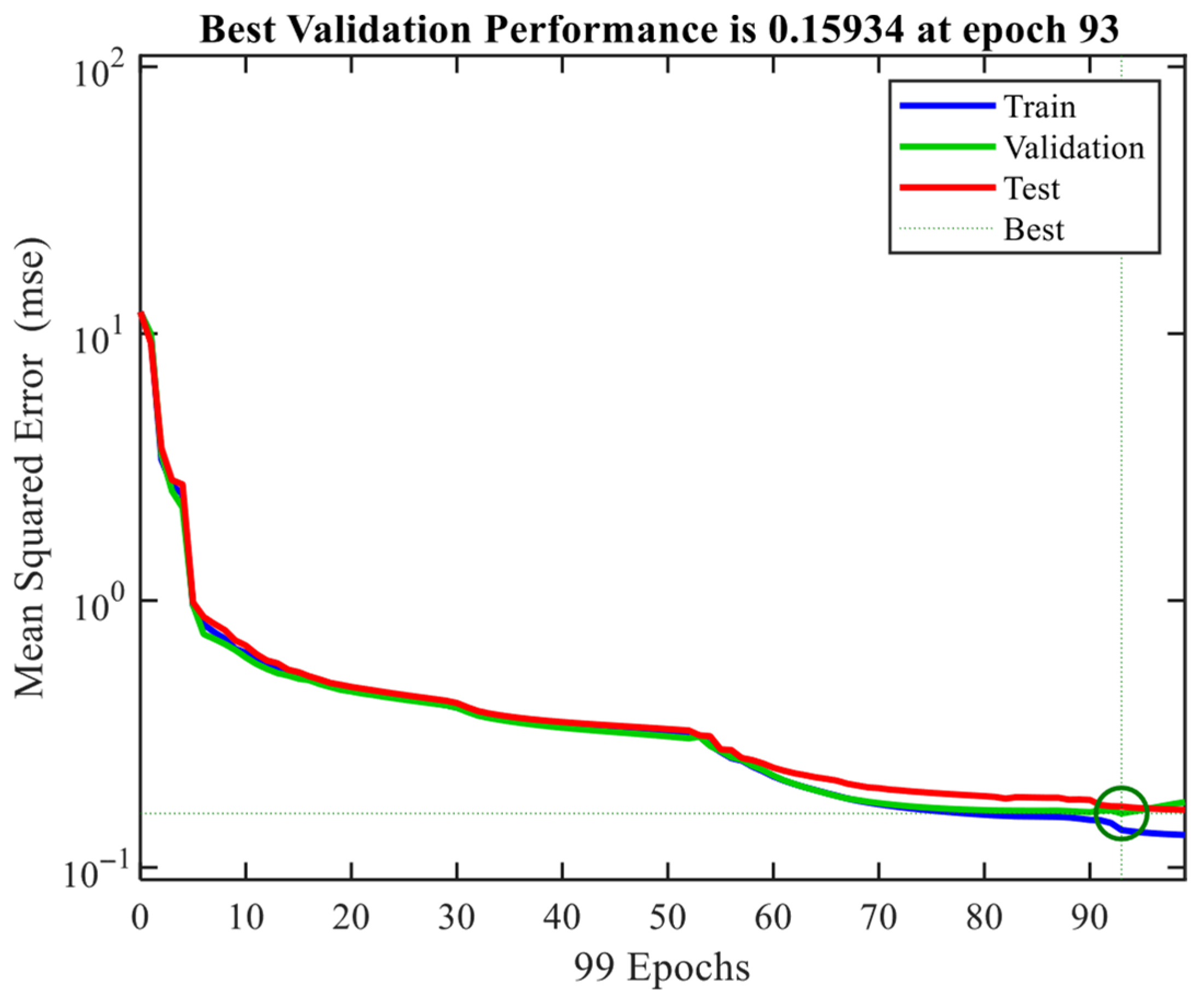
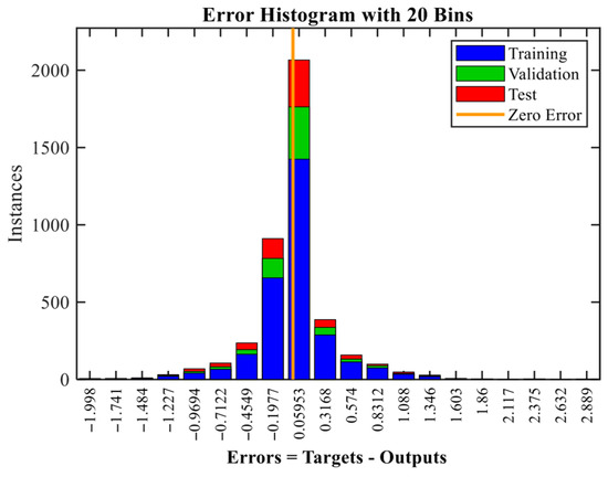
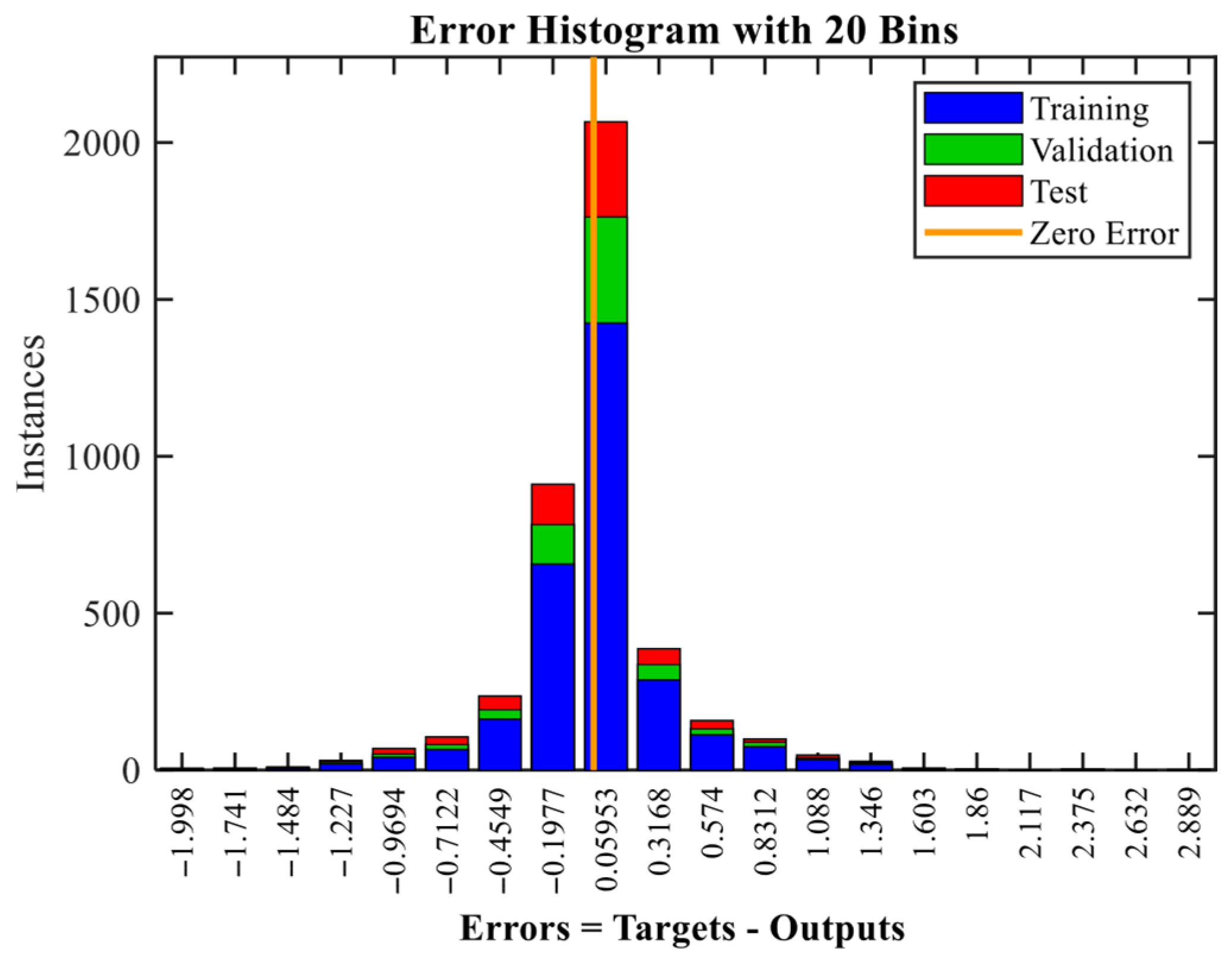
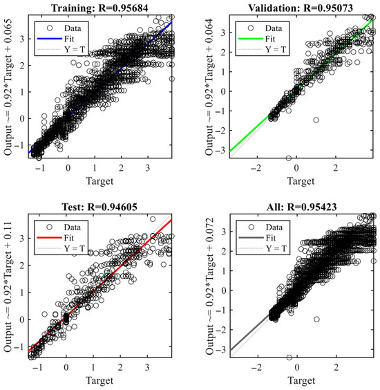
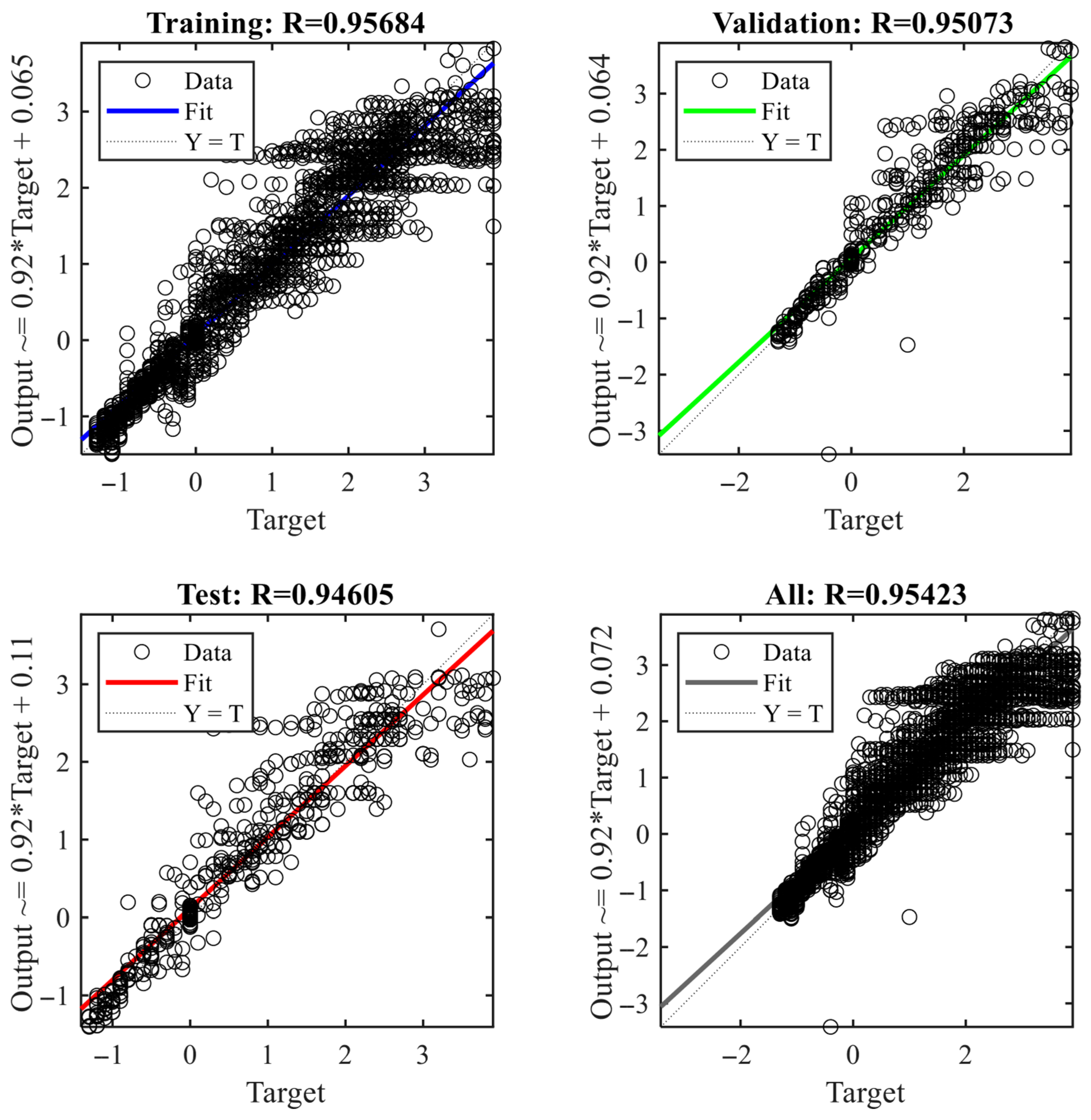
The total number of samples in the training dataset is 3600, with the training set, validation set, and test set accounting for 70%, 15%, and 15%, respectively. During regression training, the R² values across various datasets perform well—around 0.95—indicating that the ANN model achieves high accuracy while posing minimal risk of overfitting. The training results are shown in Figure 10, Figure 11 and Figure 12. To ensure the model possesses strong generalization capabilities and avoids overfitting the training data, an independent validation set—comprising 15% of the total samples—was utilized to monitor the training process through an early stopping mechanism, as shown in Figure 10.

Figure 10. Best validation performance.

Figure 11. Error histogram.

Figure 12. Training, validation, and test results.

4. Simulation Results Analysis

In this study, the two proposed automatic calibration strategies are validated: a rule-based strategy and an ANN-based strategy. All the simulations are performed under Matlab/Simulink, with the same conditions as the training datasets for the ANN model.

During the simulation, the same operating condition as the training dataset is selected—20% throttle and gear shift in D1D2. Initial parameters ($P_{OCBase}^1$ and $P_{OGBase}^1$) are set. After each gear shift, the calibration parameters should be updated as:

$$P_{OCBase}^{i+1}=P_{OCBase}^i-{∆P}_{OCBase}^i$$

(46)

$$P_{OGBase}^{i+1}=P_{OGBase}^i-{∆P}_{OGBase}^i$$

(47)

$P_{OCBase}^i$ and $P_{OGBase}^i$ are the values in the current gear shift; ${∆P}_{OCBase}^i$ and ${∆P}_{OGBase}^i$ are the adjusted values in the current gear shift based on the calibration strategy; $P_{OCBase}^{i+1}$ and $P_{OGBase}^{i+1}$ are the values in the next gear shift.

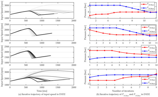
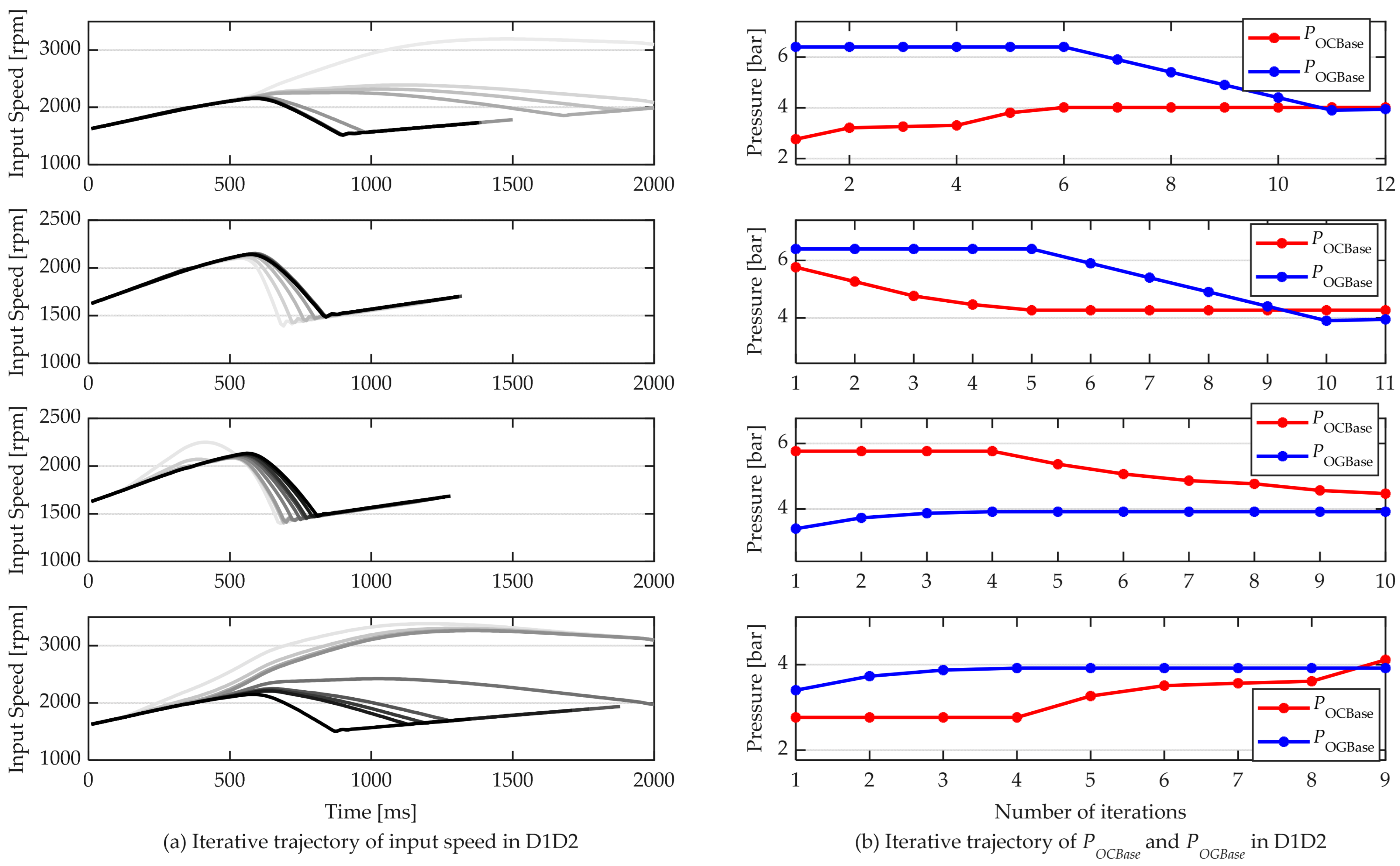
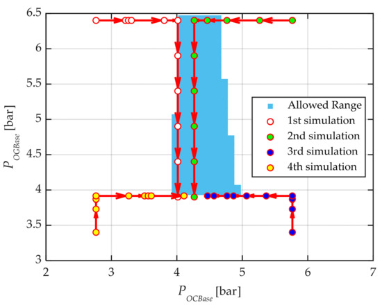
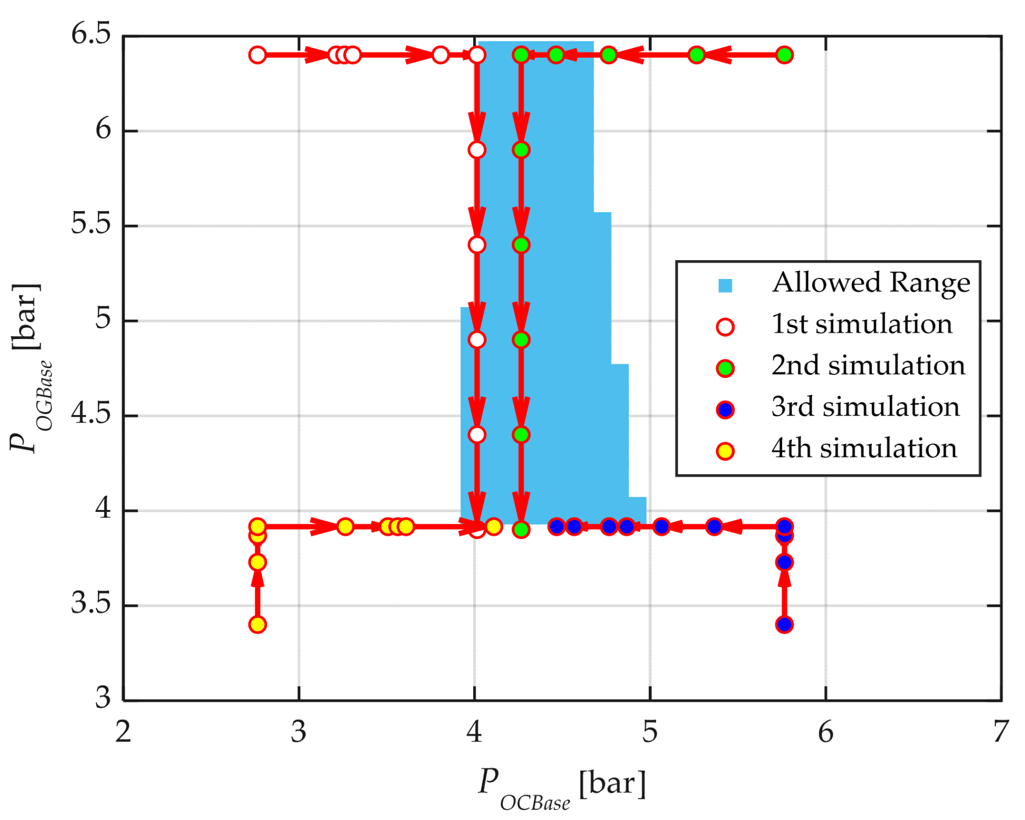
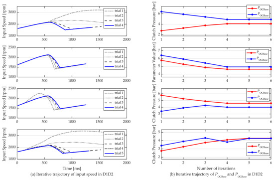
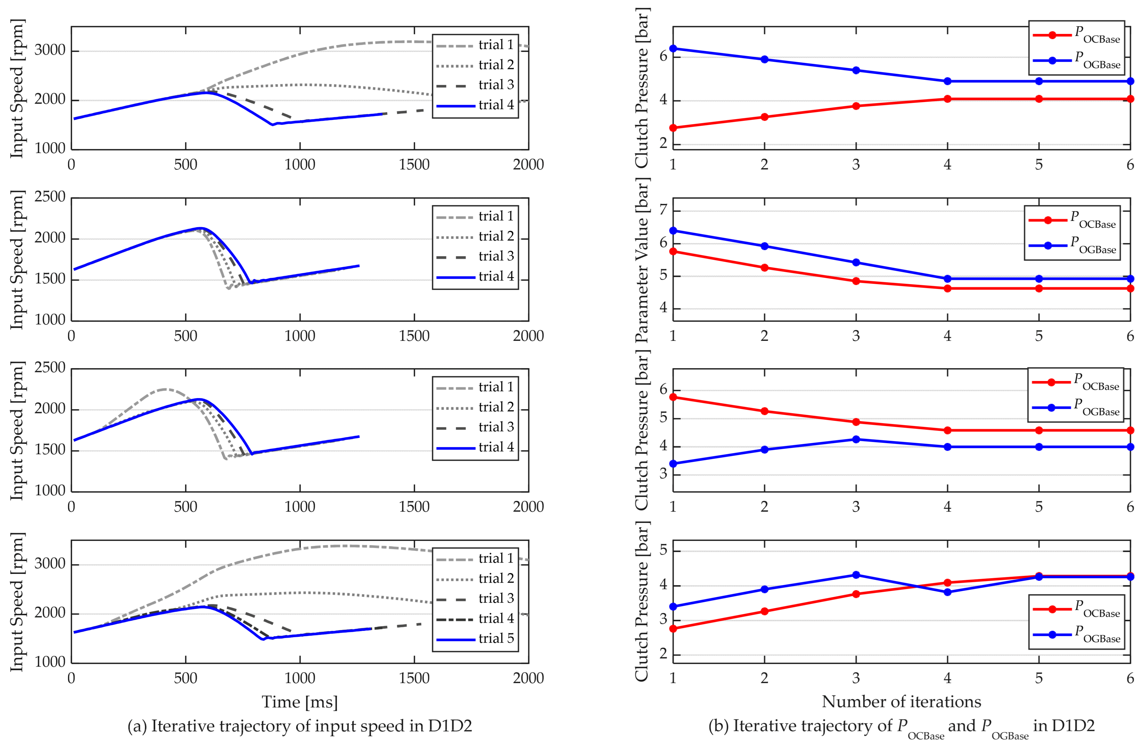
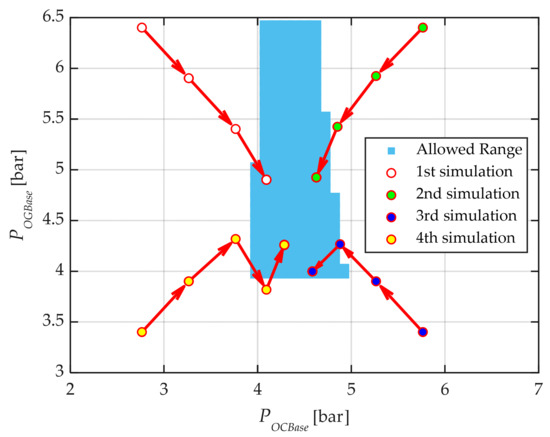
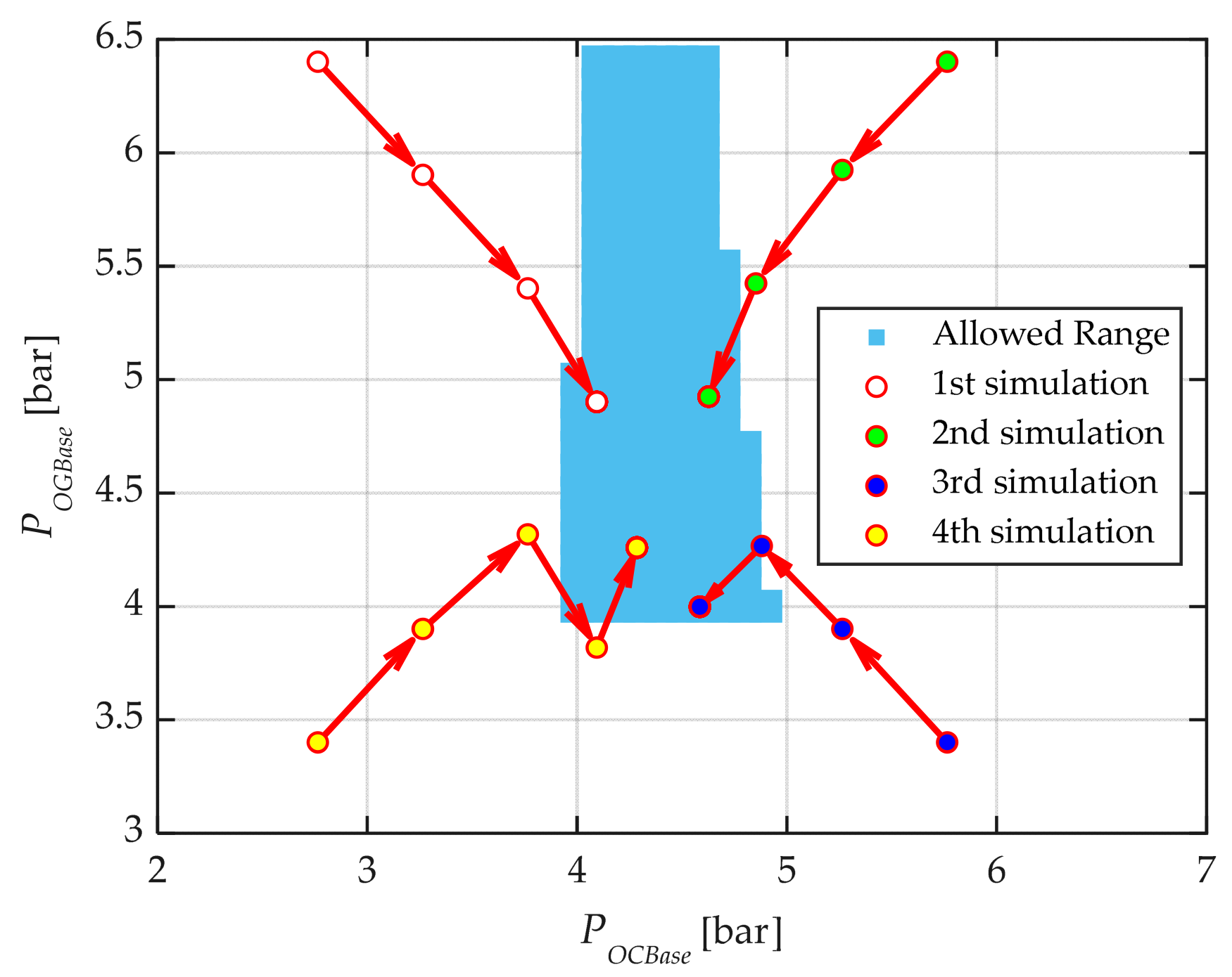
For the rule-based strategy, four simulations were conducted by setting different initial values for $P_{OCBase}$ and $P_{OGBase}$. Figure 13 shows the simulation results. Figure 13a is the iterative trajectory of input speed (as the number of iterations increases, the color of the lines deepens). Figure 13b is the iterative trajectory of $P_{OCBase}$ and $P_{OGBase}$. As shown in Figure 14, after approximately 10 iterations, both parameters starting from different initial points are able to reach the allowed range that satisfies engineering experience.

Figure 13. Simulation results in D1D2 with different initial values for the rule-based strategy.

Figure 14. Iteration trajectories in 4 simulations for the rule-based strategy.

Table 2 shows the exact initial and final values in the four simulations. Figure 14 shows that $P_{OGBase}$ can reach the min value, which could hold the input torque transmitted by the OG clutch. The allowed range is the convergence interval of $P_{OCBase}$ and $P_{OGBase}$, which is obtained from the dataset shown in Figure 8, taking into account the constraints of Equation (45).

Table 2. Initial and final values in 4 simulations for the rule-based strategy.

Simulations	${\mathit{P}}_{\mathit{O}\mathit{C}\mathit{B}\mathit{a}\mathit{s}\mathit{e}}^{\mathit{I}\mathit{n}\mathit{i}\mathit{t}}$ [bar]	${\mathit{P}}_{\mathit{O}\mathit{G}\mathit{B}\mathit{a}\mathit{s}\mathit{e}}^{\mathit{I}\mathit{n}\mathit{i}\mathit{t}}$ [bar]	Iterations	${\mathit{P}}_{\mathit{O}\mathit{C}\mathit{B}\mathit{a}\mathit{s}\mathit{e}}^{\mathit{F}\mathit{i}\mathit{n}\mathit{a}\mathit{l}}$ [bar]	${\mathit{P}}_{\mathit{O}\mathit{G}\mathit{B}\mathit{a}\mathit{s}\mathit{e}}^{\mathit{F}\mathit{i}\mathit{n}\mathit{a}\mathit{l}}$ [bar]
1st	2.76	6.4	12	4.01	3.90
2nd	5.76	6.4	11	4.27	3.90
3rd	5.76	3.4	10	4.47	3.92
4th	2.76	3.4	9	4.11	3.92

The trained ANN model is integrated into the simulation model for automatic calibration testing, and the testing process is shown in Figure 7. During the simulation, the same operating condition as the training dataset is selected—20% throttle and gear shift in D1D2, and initial parameters ($P_{OCBase}^1$ and $P_{OGBase}^1$) are set. During the simulation, to prevent overshoot, set limit of 0.5 bar for the output results (${∆P}_{OCBase}$ and ${∆P}_{OGBase}$) of the ANN model.

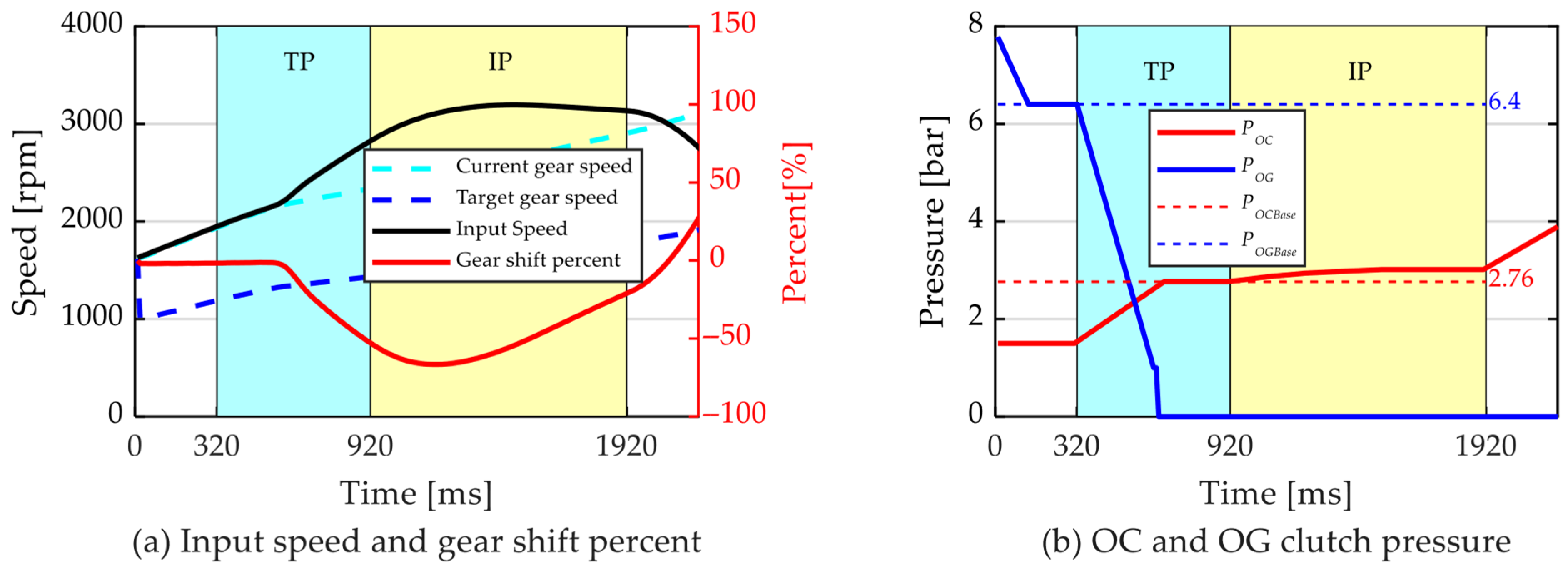
In the first simulation, the initial value of $P_{OCBase}^1$ is set to a smaller value of 2.76 bar, and the initial value of $P_{OGBase}^1$ is set to a larger value of 6.4 bar. Figure 15 and Figure 16 show the trajectories of input shaft speed, gear-shift percentage, and clutch pressure during several iterations. It can be seen that the ANN model adjusted the gear shift quality to a normal level within only four iterations. Figure 15a,b are simulation results for the initial values, where the gear shift process exhibits significant abnormalities. The input shaft exhibits severe flare during TP, but does not flare during FP, indicating that $P_{OCBase}^1$ is small while $P_{OCGBase}^1$ is not small. Since the OC clutch is unable to fully transmit the input shaft torque, the flare is severe. As the shift process fails to meet the conditions for normal completion of TP and IP, TP and IP must be forcibly terminated, causing both the duration of TP and IP to reach their maximum values. Finally, the feature matrix extracted from the first iteration of the gear shift process is [0, −53, 600, 1000], the outputs of the ANN model are [−0.5, 0.5], indicating that ${∆P}_{OCBase}$ needs to add 0.5 bar, while ${∆P}_{OGBase}$ needs to minus 0.5 bar.

Figure 15. Simulation results of the 1st iteration for the ANN-based strategy.

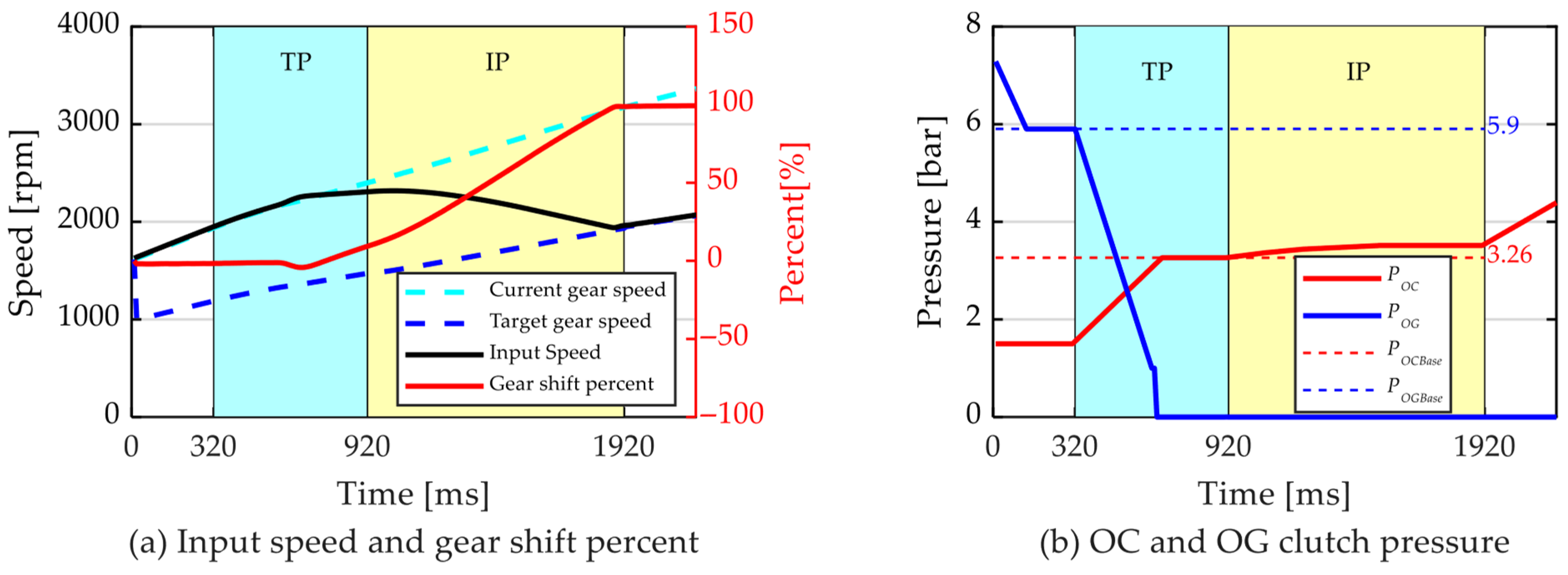
Figure 16. Simulation results of the 2nd iteration for the ANN-based strategy.

After adjustment, in the second iteration, ${∆P}_{OCBase}$ became 3.26 bar, and ${∆P}_{OGBase}$ became 5.9 bar. The second iteration simulation results are shown in Figure 16a,b. The severity of flare decreased, but the durations of the TP and IP remained at their maximum values. The feature matrix for gear shift is [0, −4.2, 600, 1000], the outputs of the ANN model are [−0.5, 0.5], indicating that ${∆P}_{OCBase}$ needs to add 0.5 bar, while ${∆P}_{OGBase}$ needs to minus 0.5 bar.

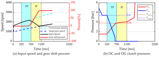
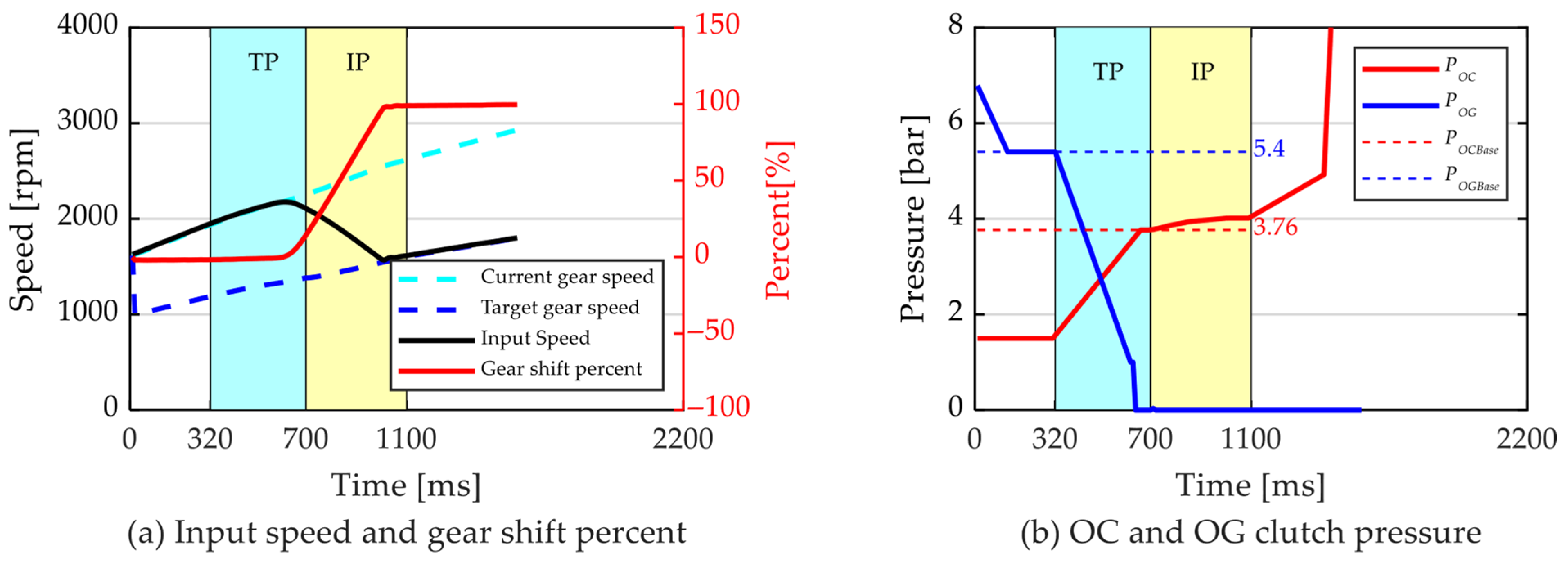
Before the third iteration, ${∆P}_{OCBase}$ became 3.76 bar, and ${∆P}_{OGBase}$ became 5.4 bar. The third iteration simulation results are shown in Figure 17a,b. The flare disappeared, while the duration of TP and IP was still long. The feature matrix for gear shift is [0, 0, 380, 410], the outputs of the ANN model are [−0.33, 0.5], indicating that ${∆P}_{OCBase}$ needs to add 0.33 bar, while ${∆P}_{OGBase}$ needs to minus 0.5 bar.

Figure 17. Simulation results of the 3rd iteration for the ANN-based strategy.

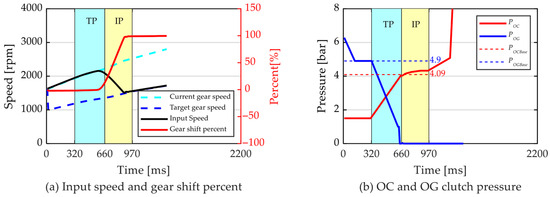
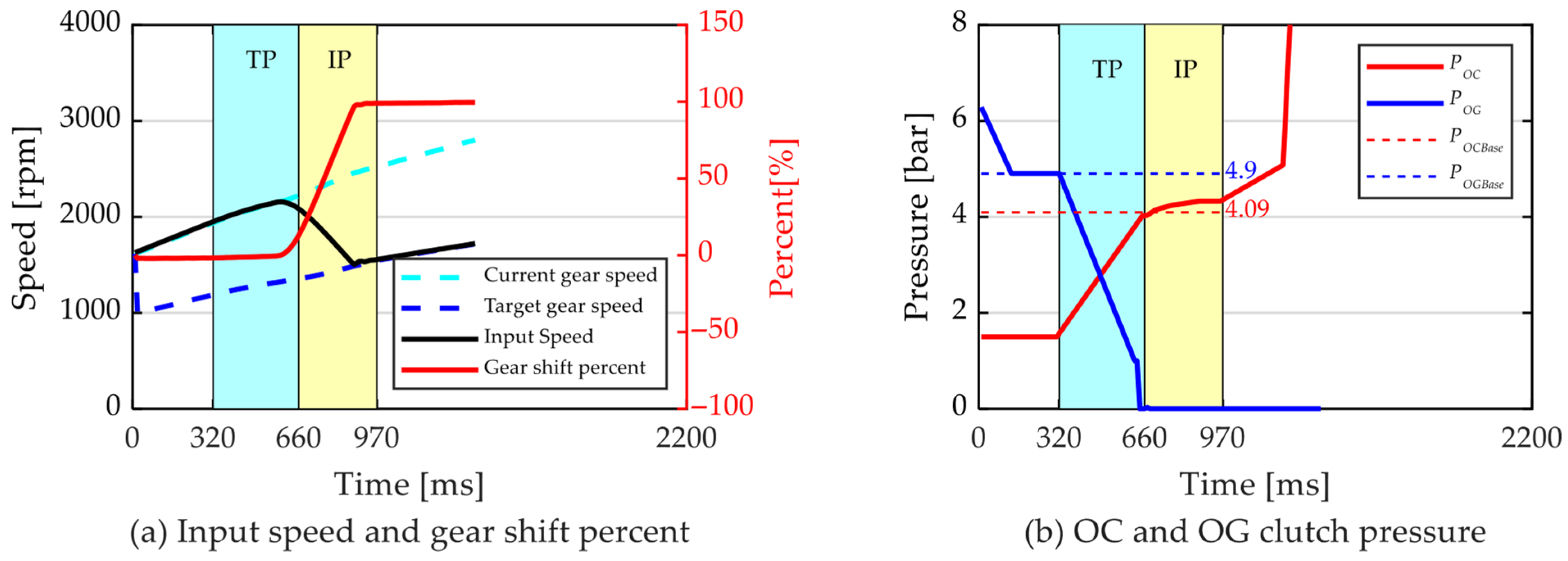
Before the fourth iteration, ${∆P}_{OCBase}$ became 4.09 bar, and ${∆P}_{OGBase}$ became 4.9 bar. The third iteration simulation results are shown in Figure 18a,b. Flare disappeared, while the duration of TP and IP is still long. The flare disappeared, and both the duration of TP and IP are within acceptable ranges, indicating that the current gearshift quality meets empirical requirements. The gear shift features and outputs of the ANN model across four iterations in the first simulation are shown in Table 3.

Figure 18. Simulation results of the 4th iteration for the ANN-based strategy.

Table 3. Iteration process of the ANN model during the first simulation for the ANN-based strategy.

Iterations	Gear Shift Features of the ANN Model				Outputs of the ANN Model		Parameters
	${\mathit{G}\mathit{S}\mathit{P}}_{\mathit{F}\mathit{l}\mathit{r}\_\mathit{F}\mathit{P}}$ [%]	${\mathit{G}\mathit{S}\mathit{P}}_{\mathit{F}\mathit{l}\mathit{r}\_\mathit{T}\mathit{P}}$ [%]	${\mathit{T}}_{\mathit{T}\mathit{P}}$ [ms]	${\mathit{T}}_{\mathit{I}\mathit{P}}$ [ms]	${∆\mathit{P}}_{\mathit{O}\mathit{C}\mathit{B}\mathit{a}\mathit{s}\mathit{e}}^{\mathit{i}}$ [bar]	${∆\mathit{P}}_{\mathit{O}\mathit{G}\mathit{B}\mathit{a}\mathit{s}\mathit{e}}^{\mathit{i}}$ [bar]	${\mathit{P}}_{\mathit{O}\mathit{C}\mathit{B}\mathit{a}\mathit{s}\mathit{e}}^{\mathit{i}}$ [bar]	${\mathit{P}}_{\mathit{O}\mathit{G}\mathit{B}\mathit{a}\mathit{s}\mathit{e}}^{\mathit{i}}$ [bar]
1st	0	−53	600	1000	−0.5	0.5	2.76	6.4
2nd	0	−4.2	600	1000	−0.5	0.5	3.26	5.9
3rd	0	0	380	410	−0.33	0.5	3.76	5.4
4th	0	0	340	310	0	0	4.09	4.9

During the other three simulations, relatively different initial values were assigned to $P_{OCBase}^1$ and $P_{OGBase}^1$. These three simulation results will no longer be analyzed in detail. Among all 4 simulations, the iteration process of input speed and calibration parameters is shown in Figure 19a,b, respectively. After 4 or 5 iterations, the gearshift quality meets empirical requirements. From the iterative process, it can be observed that after each ANN model adjustment, the input shaft speed becomes increasingly closer to the normal trajectory, and the anomaly features gradually disappear. The number of iterations and final parameter values ($P_{OCBase}^{Final}$ and $P_{OGBase}^{Final}$) under different initial values ($P_{OCBase}^{Init}$ and $P_{OGBase}^{Init}$) are shown in Table 4. The iterative trajectories of calibration parameters under different initial values are shown in Figure 20, and the final parameter values all fell within the allowed range.

Figure 19. Simulation results in D1D2 with different initial values for the ANN-based strategy.

Table 4. Initial and final values in four simulations for the ANN-based strategy.

Simulations	${\mathit{P}}_{\mathit{O}\mathit{C}\mathit{B}\mathit{a}\mathit{s}\mathit{e}}^{\mathit{I}\mathit{n}\mathit{i}\mathit{t}}$ [bar]	${\mathit{P}}_{\mathit{O}\mathit{G}\mathit{B}\mathit{a}\mathit{s}\mathit{e}}^{\mathit{I}\mathit{n}\mathit{i}\mathit{t}}$ [bar]	Iterations	${\mathit{P}}_{\mathit{O}\mathit{C}\mathit{B}\mathit{a}\mathit{s}\mathit{e}}^{\mathit{F}\mathit{i}\mathit{n}\mathit{a}\mathit{l}}$ [bar]	${\mathit{P}}_{\mathit{O}\mathit{G}\mathit{B}\mathit{a}\mathit{s}\mathit{e}}^{\mathit{F}\mathit{i}\mathit{n}\mathit{a}\mathit{l}}$ [bar]
1st	2.76	6.4	4	4.09	4.90
2nd	5.76	6.4	4	4.63	4.92
3rd	5.76	3.4	4	4.58	4.00
4th	2.76	3.4	5	4.29	4.26

Figure 20. Iteration trajectories in four simulations for the ANN-based strategy.

The rule-based strategy had an average iteration count of 10.5, while the ANN-based strategy had an average iteration count of 4.25. Compared with the rule-based strategy, the ANN-based strategy achieved a 60% improvement in convergence speed.

Since the ANN model in this paper was trained based on datasets of D1D2 gear shift at 20% throttle, automatic calibration for D1D2 achieves satisfactory results as expected. To further verify the generalization ability of the proposed ANN model, simulations under other operating conditions—such as different throttle levels and gears—are required.

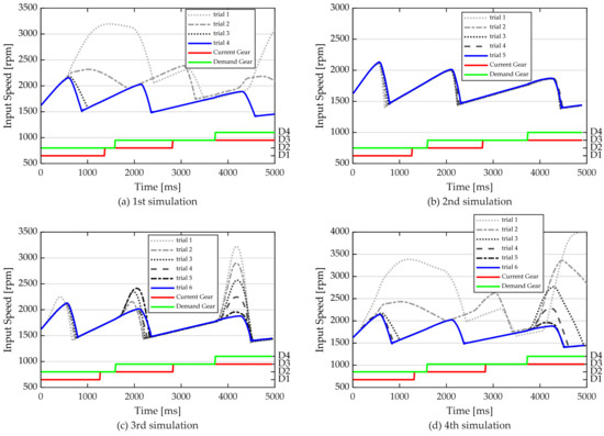
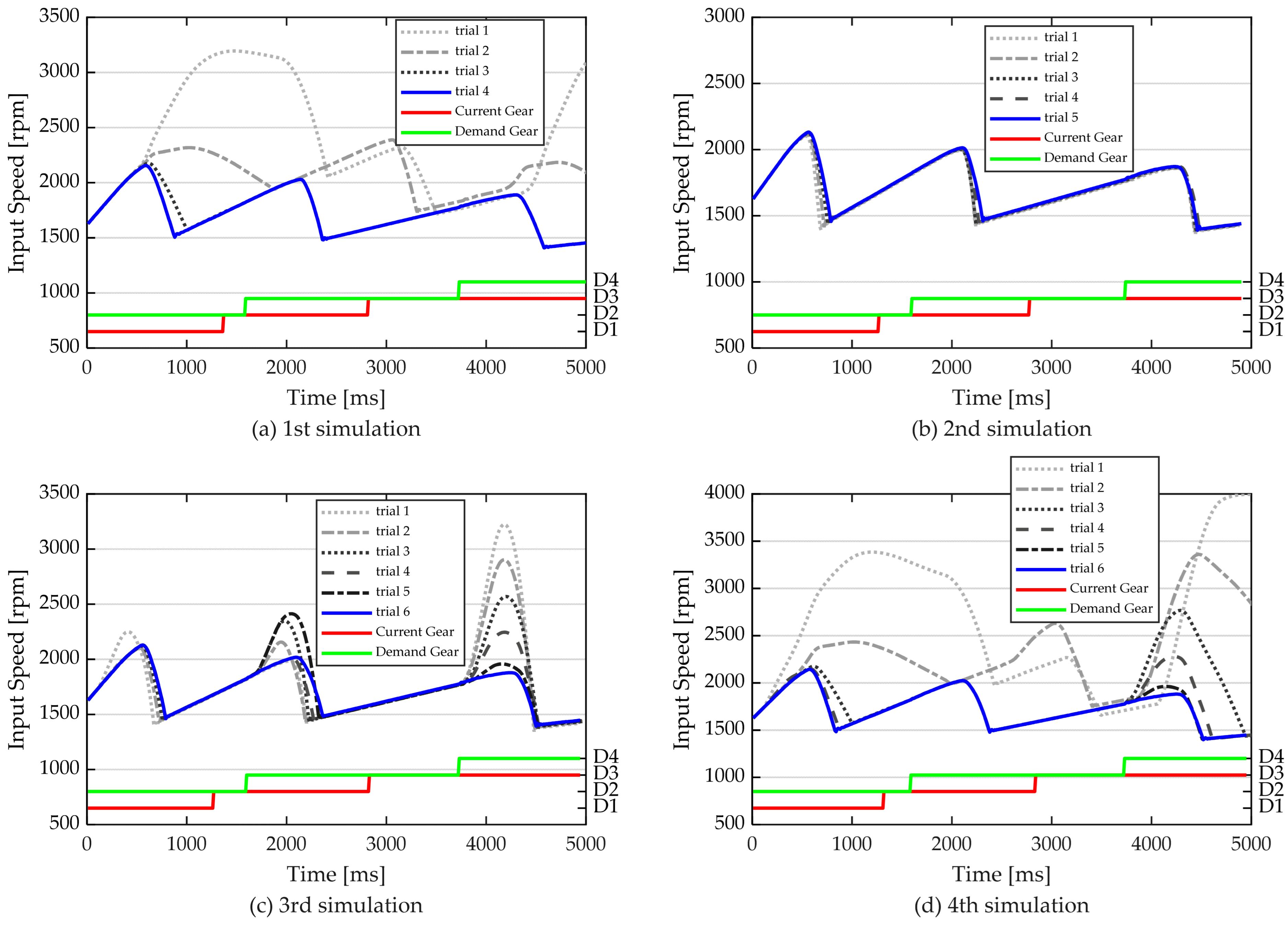
Figure 21 shows the iterative process of D1D2, D2D3, and D3D4 gear shifts at 20% throttle. It can be seen that under different initial parameters ((a) $P_{OCBase}^{Init}$ is small, $P_{OGBase}^{Init}$ is small; (b) $P_{OCBase}^{Init}$ is small, $P_{OGBase}^{Init}$ is large; (c) $P_{OCBase}^{Init}$ is large, $P_{OGBase}^{Init}$ is small; (d) $P_{OCBase}^{Init}$ is large, $P_{OGBase}^{Init}$ is large), gear shift quality can be adjusted to meet engineering experience requirements in up to six iterations.

Figure 21. Simulation results with 20% pedal for the ANN-based strategy.

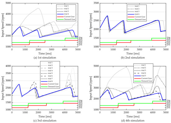
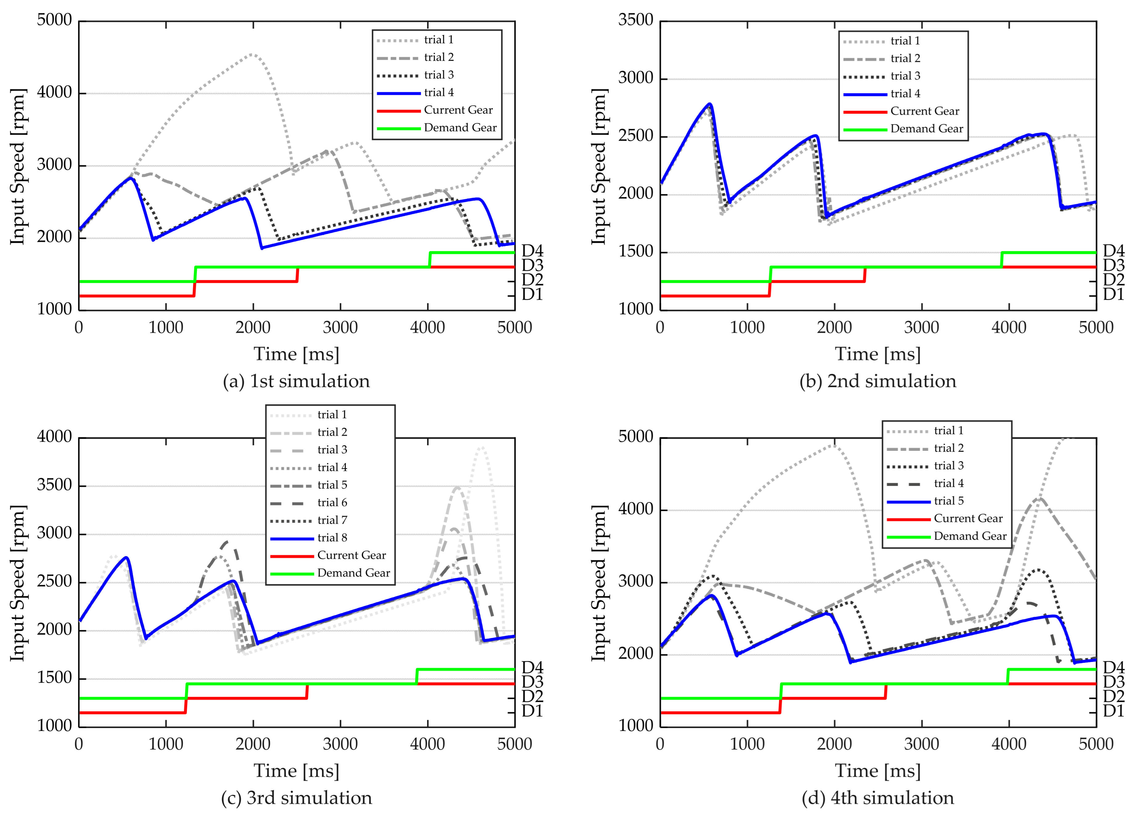
Figure 22 shows the iterative process of D1D2, D2D3, and D3D4 gear shifts at 50% throttle. It can be seen that under different initial parameters ((a) $P_{OCBase}^{Init}$ is small, $P_{OGBase}^{Init}$ is small; (b) $P_{OCBase}^{Init}$ is small, $P_{OGBase}^{Init}$ is large; (c) $P_{OCBase}^{Init}$ is large, $P_{OGBase}^{Init}$ is small; (d) $P_{OCBase}^{Init}$ is large, $P_{OGBase}^{Init}$ is large), gear shift quality can be adjusted to meet engineering experience requirements in up to eight iterations.

Figure 22. Simulation results with 50% pedal for the ANN-based strategy.

5. Conclusions

This study proposes an ANN–based automatic calibration method for AT. The ANN model incorporates engineering calibration experience and automatically adjusts parameters by monitoring key features of the gear shift process—determining whether relevant parameters are too large or too small. Importantly, this method does not rely on high-precision math models or complex control algorithms; instead, it achieves the desired performance using only a large volume of training data. The following studies have been completed:

(1)

Engineers’ calibration experience has been codified into a rule-based automatic calibration strategy that can optimize shift metrics to target values within approximately 10 iterations.

(2)

Iterate through calibration parameters to collect a large amount of gear shift process data, then extract gear shift features and label them for training an ANN model.

(3)

When performing automatic calibration using a trained ANN model, the calibration can be completed within a maximum of five iterations. Compared with the rule-based strategy, the convergence speed of the ANN-based strategy improved by 60%.

(4)

When the simulation conditions match those of the training dataset, the iterative process converges rapidly; however, under other differing conditions, the convergence rate slows, indicating that the ANN model possesses a degree of generalization. To improve the performance of the ANN model, it is necessary to expand the range of conditions represented in the training dataset.

The automatic calibration strategy proposed in this paper eliminates reliance on highly accurate AT models. It captures the shift characteristics of AT and trains an ANN model to learn the mapping between these shift characteristics and calibration parameters. During automatic calibration, compared to the rule-based strategy, this ANN model can rapidly adjust calibration parameters to allowed ranges within just a few iterations, satisfying empirical shift-quality requirements. Moreover, even under operating conditions and shifting scenarios that differ from the training dataset, the ANN-based strategy still demonstrates performance no worse than that of rule-based strategies, exhibiting a degree of adaptability and considerable potential for optimization. Compared with conventional manual calibration methods and other model-based automatic calibration approaches, the characteristic-based automatic calibration method proposed herein enhances calibration efficiency, shortens calibration cycles, and holds potential for generalization ability. Because the ANN model is effective only on the training dataset, and the shifting data from the real vehicle differs substantially from the shifting data of the simulation model, this study could not perform on-vehicle validation. The ANN model’s generalization capability and its application to real vehicles will be the focus of future research.

References

- Masunaga, S.; Miyazaki, T.; Habata, Y.; Yamada, K.; Hasegawa, Y.; Kondo, T.; Kitaori, I.; Takeichi, A. Development of Innovative Toyota 10-Speed Longitudinal Automatic Transmission. SAE Int. J. Engines 2017, 10, 701–708. [Google Scholar] [CrossRef] [Scilit]
- Küçükay, F.; Kassel, T.; Alvermann, G.; Gartung, T. Efficient Calibration of Automatic Transmissions on the Roller Dynamometer. ATZ Worldw. 2009, 111, 46–52. [Google Scholar] [CrossRef] [Scilit]
- Mishra, K.D.; Cardwell, G.; Srinivasan, K. Automated Calibration of Gearshift Controllers Using Iterative Learning Control for Hybrid Systems. Control Eng. Pract. 2021, 111, 104786. [Google Scholar] [CrossRef] [Scilit]
- Yanakiev, D.; Fujii, Y.; Tseng, E.; Pietron, G.M.; Kucharski, J.; Kapas, N. Torque Phase Shift Control Based on Clutch Torque Estimation. In Proceedings of the ASME 2013 Dynamic Systems and Control Conference, Palo Alto, CA, USA, 21–23 October 2013; Volume 1, p. V001T11A004. [Google Scholar]
- Kim, S.; Oh, J.J.; Choi, S.B. Driveline Torque Estimations for a Ground Vehicle with Dual-Clutch Transmission. IEEE Trans. Veh. Technol. 2018, 67, 1977–1989. [Google Scholar] [CrossRef] [Scilit]
- Cvok, I.; Deur, J.; Ivanovic, V.; Zhang, Y.; Fujii, Y. Optimal Control Allocation-Based Automatic Transmission Upshift Control Strategy for Inertia Phase. IEEE Trans. Veh. Technol. 2024, 73, 1957–1973. [Google Scholar] [CrossRef] [Scilit]
- Thornton, S.; Annaswamy, A.; Yanakiev, D.; Pietron, G.M.; Riedle, B.; Filev, D.; Wang, Y. Adaptive Shift Control for Automatic Transmissions. In Proceedings of the ASME 2014 Dynamic Systems and Control Conference, San Antonio, TX, USA, 22–24 October 2014; Volume 2, p. V002T27A001. [Google Scholar]
- Bagot, B.; Schmidt, A.; Ebner, T.; Altenstrasser, H. Model-Based Methodology for the Automated Optimization of Shift Quality for Automatic Transmissions. ATZ Worldw. 2008, 110, 12–17. [Google Scholar] [CrossRef] [Scilit]
- Steffen, B. Reproducible Shifting Points and Automated Calibration of Passenger Cars’ Transmissions. ATZ Worldw. 2007, 109, 9–12. [Google Scholar] [CrossRef] [Scilit]
- Boissinot, F.; Bellavoine, J.; Shabashevich, A.; Puster, S. Automated Calibration for Transmission on Powertrain Dynamometers. In SAE Technical Paper; SAE International: Detroit, MI, USA, 2015. [Google Scholar] [CrossRef] [Scilit]
- Wu, J.; Walker, P.D.; Ruan, J.; Zhang, N. Target Torque Estimation for Gearshift in Dual Clutch Transmission with Uncertain Parameters. Appl. Math. Model. 2017, 51, 1–20. [Google Scholar] [CrossRef] [Scilit]
- Zhou, S.; Walker, P.; Wu, J.; Zhang, N. Power on Gear Shift Control Strategy Design for a Parallel Hydraulic Hybrid Vehicle. Mech. Syst. Signal Process. 2021, 159, 107798. [Google Scholar] [CrossRef] [Scilit]
- Roozegar, M.; Setiawan, Y.D.; Angeles, J. Design, Modelling and Estimation of a Novel Modular Multi-Speed Transmission System for Electric Vehicles. Mechatronics 2017, 45, 119–129. [Google Scholar] [CrossRef] [Scilit]
- Zhao, Z.; He, L.; Yang, Y.; Wu, C.; Li, X.; Karl Hedrick, J. Estimation of Torque Transmitted by Clutch during Shifting Process for Dry Dual Clutch Transmission. Mech. Syst. Signal Process. 2016, 75, 413–433. [Google Scholar] [CrossRef] [Scilit]
- Wu, J.; Zhou, S.; Zhang, Y.; Zhou, S. Optimal Gear Shift Control of Two-Speed Dual-Clutch Transmission in Electric Vehicle for Smoothness and Friction Loss Reduction. Int. J. Automot. Technol. 2024, 25, 913–930. [Google Scholar] [CrossRef] [Scilit]
- Tian, Y.; Yang, H.; Mo, W.; Zhou, S.; Zhang, N.; Walker, P.D. Optimal Coordinating Gearshift Control of a Two-Speed Transmission for Battery Electric Vehicles. Mech. Syst. Signal Process. 2020, 136, 106521. [Google Scholar] [CrossRef] [Scilit]
- Mishra, K.D.; Srinivasan, K. Robust Control and Estimation of Clutch-to-Clutch Shifts. Control Eng. Pract. 2017, 65, 100–114. [Google Scholar] [CrossRef] [Scilit]
- Zhao, Z.; Li, X.; He, L.; Wu, C.; Hedrick, J.K. Estimation of Torques Transmitted by Twin-Clutch of Dry Dual-Clutch Transmission during Vehicle’s Launching Process. IEEE Trans. Veh. Technol. 2017, 66, 4727–4741. [Google Scholar] [CrossRef] [Scilit]
- Oh, J.J.; Choi, S.B.; Kim, J. Driveline Modeling and Estimation of Individual Clutch Torque during Gear Shifts for Dual Clutch Transmission. Mechatronics 2014, 24, 449–463. [Google Scholar] [CrossRef] [Scilit]
- Čorić, M.; Ranogajec, V.; Deur, J.; Ivanović, V.; Eric Tseng, H. Optimization of Shift Control Trajectories for Step Gear Automatic Transmissions. J. Dyn. Syst. Meas. Control 2017, 139, 061005. [Google Scholar] [CrossRef] [Scilit]
- Ranogajec, V.; Deur, J.; Coric, M. Bond Graph Analysis of Automatic Transmission Shifts Including Potential of Extra Clutch Control. SAE Int. J. Engines 2016, 9, 1929–1945. [Google Scholar] [CrossRef] [Scilit]
- Feng, J.; Qin, D.; Liu, Y.; Wang, X.; Lv, H. Pseudo-Spectral Optimization and Data-Driven Control of Vehicle Start Process with Dual-Clutch Transmission. Mech. Mach. Theory 2022, 172, 104814. [Google Scholar] [CrossRef] [Scilit]
- Liu, Y.; Zhang, J.; Lv, Z.; Ye, J. The Optimization of RBFNN Gearshift Controller Parameters for Electric Vehicles Using PILCO Reinforcement Learning. IEEE Access 2023, 11, 92807–92821. [Google Scholar] [CrossRef] [Scilit]
- Xia, G.; Chen, J.; Tang, X.; Zhao, L.; Sun, B. Shift Quality Optimization Control of Power Shift Transmission Based on Particle Swarm Optimization–Genetic Algorithm. Proc. Inst. Mech. Eng. Part D J. Automob. Eng. 2022, 236, 872–892. [Google Scholar] [CrossRef] [Scilit]
- Liu, Z.; Gao, J.; Zheng, Q. Antishudder Gearshift Controller Design for Automatic Transmission. IEEE Trans. Veh. Technol. 2011, 60, 4261–4275. [Google Scholar] [CrossRef] [Scilit]
- Li, A.; Qin, D. Adaptive Model Predictive Control of Dual Clutch Transmission Shift Based on Dynamic Friction Coefficient Estimation. Mech. Mach. Theory 2022, 173, 104804. [Google Scholar] [CrossRef] [Scilit]
- Park, J.; Choi, S. Gear Shifting Based on MIMO Model Predictive Control for Convenient Adjustment of Shifting Performance. IEEE Trans. Veh. Technol. 2022, 71, 233–249. [Google Scholar] [CrossRef] [Scilit]
- Cvok, I.; Soldo, J.; Deur, J.; Ivanovic, V.; Zhang, Y.; Fujii, Y. Model Predictive Control for Automatic Transmission Upshift Inertia Phase. IEEE Trans. Contr. Syst. Technol. 2023, 31, 2335–2349. [Google Scholar] [CrossRef] [Scilit]
- Cvok, I.; Soldo, J.; Deur, J.; Ivanovic, V.; Zhang, Y.; Fujii, Y. Integrated Torque and Inertia Phase Model Predictive Controls of Automatic Transmission Upshifts. IEEE Trans. Veh. Technol. 2025, 74, 12072–12088. [Google Scholar] [CrossRef] [Scilit]
- Cvok, I.; Deur, J.; Ivanovic, V.; Zhang, Y.; Fujii, Y. An LQR Approach of Automatic Transmission Upshift Control Including Use of Off-Going Clutch within Inertia Phase. SAE Int. J. Adv. Curr. Prac. Mobil. 2020, 2, 2081–2091. [Google Scholar] [CrossRef] [Scilit]
- Lu, X.; Chen, H.; Gao, B.; Zhang, Z.; Jin, W. Data-Driven Predictive Gearshift Control for Dual-Clutch Transmissions and FPGA Implementation. IEEE Trans. Ind. Electron. 2015, 62, 599–610. [Google Scholar] [CrossRef] [Scilit]
- Mishra, K.D.; Cardwell, G.; Srinivasan, K. Modeling, Control, and Adaptation for Shift Quality Control of Automatic Transmissions. In SAE Technical Paper Series; SAE International: Warrendale, PA, USA, 2019. [Google Scholar] [CrossRef] [Scilit]
- Shin, S.; Choi, S.B. Observer-Based Iterative Learning Control for a High Relative Degree Nonlinear System and Its Application to a Vehicular Wet-Clutch System. Mech. Mach. Theory 2023, 180, 105158. [Google Scholar] [CrossRef] [Scilit]
- Dong, P.; Li, J.; Guo, W.; Wang, S.; Xu, X.; Mao, F.; Liu, Y. Gearshift Overlap for Multistep Downshift of Automatic Transmissions Based on Iterative Learning Control. IEEE/ASME Trans. Mechatron. 2024, 29, 224–236. [Google Scholar] [CrossRef] [Scilit]
- Beaudoin, M.-A.; Boulet, B. Improving Gearshift Controllers for Electric Vehicles with Reinforcement Learning. Mech. Mach. Theory 2022, 169, 104654. [Google Scholar] [CrossRef] [Scilit]
- Jeffrey, K.R.; Kevin, L.K.; Scott, T.K. Method of Determining Initial Transmission Calibration. US7069767B2, 4 July 2006. [Google Scholar]
- Peng, H.; Maguire, J.M.; Bai, S. Dynamic Analysis and Control System Design of Automatic Transmissions; SAE International: Warrendale, PA, USA, 2013. [Google Scholar]
- Deur, J.; Asgari, J.; Hrovat, D.; Kovač, P. Modeling and Analysis of Automatic Transmission Engagement Dynamics-Linear Case. J. Dyn. Syst. Meas. Control 2006, 128, 263–277. [Google Scholar] [CrossRef] [Scilit]
- Thornton, S.; Pietron, G.M.; Yanakiev, D.; McCallum, J.; Annaswamy, A. Hydraulic Clutch Modeling for Automotive Control. In Proceedings of the 52nd IEEE Conference on Decision and Control, Florence, Italy, 10–13 December 2013; pp. 2828–2833. [Google Scholar] [CrossRef] [Scilit]
- Shi, G.; Dong, P.; Sun, H.Q.; Liu, Y.; Cheng, Y.J.; Xu, X.Y. Adaptive Control of the Shifting Process in Automatic Transmissions. Int. J. Automot. Technol. 2017, 18, 179–194. [Google Scholar] [CrossRef] [Scilit]
- Robinette, D.; Gibson, G.; Szpara, D.; Tehansky, E. Performance Characterization of Automatic Transmission Upshifts with Reduced Shift Times. SAE Int. J. Engines 2015, 8, 1359–1373. [Google Scholar] [CrossRef] [Scilit]
- Kim, D.; Peng, H.; Bai, S.; Maguire, J.M. Control of Integrated Powertrain with Electronic Throttle and Automatic Transmission. IEEE Trans. Contr. Syst. Technol. 2007, 15, 474–482. [Google Scholar] [CrossRef] [Scilit]
- Tokura, T.; Asami, T.; Hasegawa, Y.; Sugimura, T.; Kono, K.; Aoki, K. Development of Smooth Up-Shift Control Technology for Automatic Transmissions with Integrated Control of Engine and Automatic Transmission. In SAE World Congress & Exhibition; SAE International: Warrendale, PA, USA, 2007. [Google Scholar]
- Bai, S.; Brennan, D.; Dusenberry, D.; Tao, X.; Zhang, Z. Integrated Powertrain Control. In SAE 2010 World Congress & Exhibition; SAE International: Warrendale, PA, USA, 2010. [Google Scholar]
- Guo, W.; Liu, Y.; Zhang, J.; Xu, X. Dynamic Analysis and Control of the Clutch Filling Process in Clutch-to-clutch Transmissions. Math. Probl. Eng. 2014, 2014, 293637. [Google Scholar] [CrossRef] [Scilit]
- Meng, F.; Zhang, H.; Cao, D.; Chen, H. System Modeling and Pressure Control of a Clutch Actuator for Heavy-Duty Automatic Transmission Systems. IEEE Trans. Veh. Technol. 2016, 65, 4865–4874. [Google Scholar] [CrossRef] [Scilit]
- Watechagit, S.; Srinivasan, K. Modeling and Simulation of a Shift Hydraulic System for a Stepped Automatic Transmission. In SAE Technical Paper Series; SAE International: Warrendale, PA, USA, 2003. [Google Scholar] [CrossRef] [Scilit]
- Depraetere, B.; Pinte, G.; Swevers, J. A Reference Free Iterative Learning Strategy for Wet Clutch Control. In Proceedings of the 2011 American Control Conference, San Francisco, CA, USA, 29 June–1 July 2011; pp. 2442–2447. [Google Scholar]
- Pinte, G.; Depraetere, B.; Symens, W.; Swevers, J.; Sas, P. Iterative Learning Control for the Filling of Wet Clutches. Mech. Syst. Signal Process. 2010, 24, 1924–1937. [Google Scholar] [CrossRef] [Scilit]
Disclaimer/Publisher’s Note: The statements, opinions and data contained in all publications are solely those of the individual author(s) and contributor(s) and not of MDPI and/or the editor(s). MDPI and/or the editor(s) disclaim responsibility for any injury to people or property resulting from any ideas, methods, instructions or products referred to in the content. |
© 2026 by the authors. Licensee MDPI, Basel, Switzerland. This article is an open access article distributed under the terms and conditions of the Creative Commons Attribution (CC BY) license.