Near-Wellbore Hydraulic Fracture Characterization by In-Well Fiber Optic LF-DAS and DTS

Abstract

In-well hydraulic fracture monitoring based on joint low-frequency distributed acoustic sensing (LF-DAS)/distributed temperature sensing (DTS) enables the acquisition of optical fiber mechanical strain data, which reflect fracture propagation and rock deformation during hydraulic fracturing. This paper presents an analytical method to interpret the mechanical strain profile measured by in-well LF-DAS/DTS during the fracturing process based on strain transfer theory and the Sneddon solution for fracture propagation. The analytical method is validated by a numerical model that simulates the strain field induced by fracture propagation. The sensitivity of the fiber strain to key factors, such as fracture geometry parameters and gauge length, is analyzed. The results indicate that compressive strain in the formation adjacent to the propagating fracture remains observable from the mechanical strain profile under the low fiber lag parameter condition. The presented method is applied to analyze the mechanical strain profile measured from a fractured horizontal well. Considering the reactivation of the pre-existing fracture, the location of the fractures is identified, and the fractures’ geometric parameters are inverted. This study provides a quantitative evaluation method for fracture geometry characterization based on joint LF-DAS/DTS fracturing monitoring.

1. Introduction

LF-DAS has been widely used for real-time strain monitoring during fracturing. Compared with conventional fracturing monitoring methods, such as microseismic monitoring and tracer monitoring, LF-DAS monitoring exhibits advantages in characterizing fractures at the cluster level. LF-DAS measurements are correlated with axial strain in the fiber, which can be induced by both temperature change and mechanical deformation [1]. Generally, fiber cable is deployed behind the casing of the well adjacent to the fracturing well to record LF-DAS measurement. In the Hydraulic Fracturing Test Site 2 (HFTS-2) project in the Permian Delaware Basin, fibers were deployed in two horizontal wells and one vertical well to monitor LF-DAS strain response in both horizontal and vertical direction during the fracturing process [2]. In the Ordos Basin, LF-DAS was also deployed to acquire cross-well strain data. These data enabled the identification of the fracture hit location and observation of the pre-existing fracture reactivation event [3]. Recently, the value of the in-well LF-DAS data has become increasingly recognized by researchers. Kerr et al. [4] studied the LF-DAS strain response monitored from the treatment well during a diagnostic fracture injection test (DFIT). It was found that the strain response extended approximately 350 ft along the treatment well from perforation clusters, suggesting possible fracture propagation along the treatment well. Saw et al. [5] estimated fracture width based on the LF-DAS data acquired from the fracturing well during fracturing.

There are many studies on the interpretation of strain response monitored by LF-DAS fracturing monitoring. Zhang et al. [6] utilized the Displacement Discontinuity Method (DDM) to model the strain field around propagating fractures. The modeled strain/strain rate response patterns were consistent with field observations from HFTS-2. Wang et al. [7] simulated the vertical-direction strain rate response induced by fracture propagation using the Chevron proprietary 3D fully coupled finite element simulator to interpret the observed cross-well LF-DAS strain rate monitored by vertical fibers. Wu and Liu et al. [8,9] simulated the strain response pattern of frac-hit monitored by cross-well LF-DAS, and proposed an algorithm based on Green’s function for fracture width inversion [10]. Liu et al. [11] constructed a stochastic discrete fracture network to study the effects of natural fractures on both the hydraulic fracture network and the cross-well strain response. Hao et al. [12] utilized COMSOL Multiphysics to simulate cross-well LF-DAS strain rate response patterns under various monitoring well inclinations. Srinivasan et al. [13] employed a 3D DDM-based geo-mechanical model to simulate the strain and strain rate response at the in-well fiber location during hydraulic fracturing. The simulation results showed that simulated strain exhibited higher intensity than the field measurements. The discrepancy was mainly attributed to the model representing actual rock strain, while the field measurements reflect the strain experienced by the fiber.

The fiber packaging method can induce strain discrepancies between the host material and optical fiber, and strain transfer theory has been developed to correct this error [14]. By combining strain transfer theory with the penny-shaped fracture propagation model, Nwabueze et al. [15] presented an analytical method accounting for proppant deformation and fracture width hysteresis to improve the interpretation of strain measurements in hydraulic fracture diagnostics. The research team applied this method to evaluate the width and conductivity of the hydraulic fracture using in-well and far field [16] distributed strain sensing based on Rayleigh frequency shift (DSS-RFS) field data. Zhang et al. [17] simulated initiation and propagation of fractures in indoor multi-layered rock masses with the true triaxial fracturing physical simulation system, while strain was monitored by fibers deployed in each layer. Strain transfer theory was employed to identify the fracture propagation path, and the results obtained were highly consistent with the actual fracture morphology. Although strain transfer theory has seen limited application in petroleum engineering, existing studies indicate that its application improves the interpretation of strain measured by optical fibers.

Authors previously extracted mechanical strain data from LF-DAS measurements during fracturing through an improved strain-temperature decoupling method [18].

In this study, a method is proposed by combining strain transfer theory with a semi-infinite blade-shape fracture propagation model. The mechanical strain data acquired during a multi-cluster fracturing process were interpreted, and the fracture width and height were inversed.

2. Methods

2.1. Mechanism of In-Well LF-DAS Response During Fracturing

When coherent light propagates through a fiber segment of gauge length, the optical phase measured by a phase-based DAS instrument can be expressed as [19]

$$\varphi ={\displaystyle \frac{4\pi n{L}_{\mathrm{G}}}{{\lambda }_{\mathrm{L}}}}$$

(1)

where $\varphi$ is the optical phase in radians; λ_L is the wavelength, m; n is the refractive index, dimensionless; and L_G is the gauge length, m.

Gauge length is the measuring length of the fiber, which covers multiple spatial sampling locations. The physical property output is measured at the gauge-length level [20]. The wavelength is generally treated as a constant in the monitoring process. Accordingly, the optical phase change can be expressed as [21]

$$\mathsf{\Delta }\varphi =\varphi \left({\displaystyle \frac{\mathsf{\Delta }L}{L}}+{\displaystyle \frac{\mathsf{\Delta }n}{n}}\right)$$

(2)

where L represents the length of the optical fiber, m.

Temperature change affects fiber properties through thermal expansion and the thermo-optic effect, while axial strain on the fiber also induce changes in the refractive index [22]. According to the combined effect of the physical factors described above, Equation (2) can be expressed as

$$\mathsf{\Delta }\varphi =C_{\epsilon }{\epsilon }_{\mathrm{M}}+C_{\mathrm{T}}\mathsf{\Delta }T$$

(3)

where ε_M is the mechanical strain, m; T is temperature, °C; and C_ε and C_T are the strain and thermal coefficient, respectively, rad/(m/m) and rad/°C.

DTS is used to measure temperature values. When the fiber cable is permanently cemented behind the casing of the fracturing well to record DAS and DTS data during fracturing, the mechanical strain can be extracted from the low-frequency component of DAS measurements through a strain-temperature decoupling method. The mechanical strain data enable identification of near-wellbore fracture distribution and observation of fracture dynamic effectiveness throughout the fracturing process.

2.2. Optical Fiber Strain Forward Model in Fracturing Process

2.2.1. Strain Transfer Model

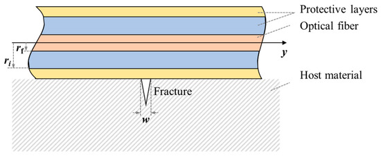
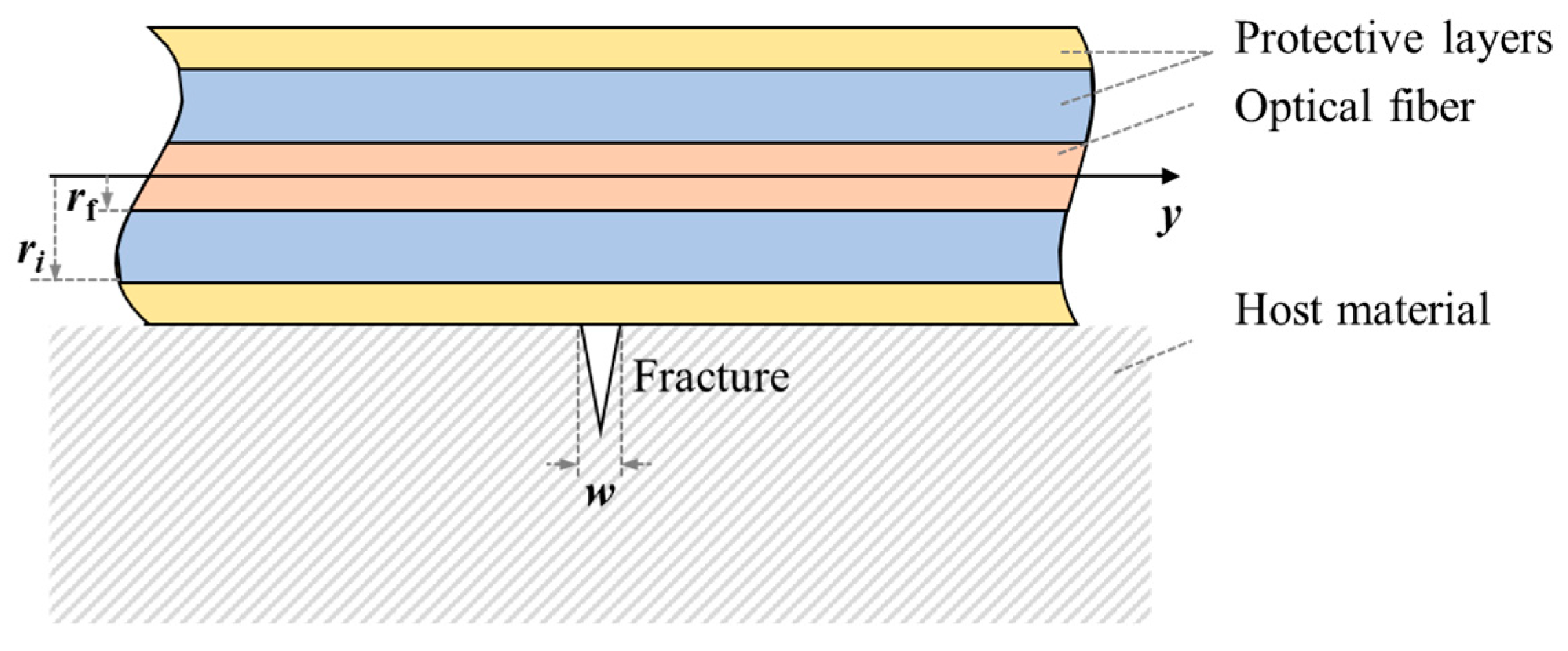
When a fracture occurs at the interface between the host material and the fiber with multi-layered protective coatings (Figure 1), the resulting deformation is transmitted through the protective layers rather than applied directly to the fiber. This transfer mechanism leads to a difference between strain measured by the fiber and the actual strain in the host material.

Figure 1. Schematic diagram of the fracture monitored by optical fiber with protective layers.

The optical fiber is treated as a linear elastic material, and the protective layers are assumed to be ideal elastoplastic materials. Perfect coupling is assumed at the interfaces between the fiber and its protective layers. The fracture is set to locate at y = 0. For any position along the fiber where y ≥ 0, there is [23,24]

$${\displaystyle \frac{{\mathrm{d}}^2{u}_{\mathrm{f}}\left(y\right)}{\mathrm{d}{y}^2}}-{\lambda }^2{u}_{\mathrm{f}}\left(y\right)=-{\lambda }^2\left[{\displaystyle \underset{0}{\overset{y}{\int }}{\epsilon }_{\mathrm{m}}\left(y^{\prime }\right)\mathrm{d}{y}^{\prime }+\frac{w}{2}}\right]$$

(4)

$${\lambda }^2={\displaystyle \frac{2}{E_{\mathrm{f}}{r}_{\mathrm{f}}^2\left[\frac{1}{G_1}\ln \left(\frac{r_1}{r_{\mathrm{f}}}\right)+{\displaystyle \sum _{i=2}^N\frac{1}{G_i}\ln \left(\frac{r_i}{r_{i-1}}\right)}\right]}}$$

(5)

where y denotes the axial coordinate along the fiber; u_f is the axial displacement of the fiber, m; λ is the fiber lag parameter, m⁻¹; ε_m denotes strain in the host material; w is the maximum fracture width, m; E is Young’s modulus, Pa; G is shear modulus, Pa; r denotes the radius of the material, m; the subscript f represents fiber, and the subscript i represents the protective layer index.

The general solution to the differential equation given in Equation (4) is expressed as

$$u_{\mathrm{f}}\left(y\right)=A\sinh (\lambda y)+B\cosh (\lambda y)+\left[{\displaystyle \underset{0}{\overset{y}{\int }}{\epsilon }_{\mathrm{m}}\left(y^{\prime }\right)\mathrm{d}{y}^{\prime }+\frac{w}{2}}\right]$$

(6)

The boundary conditions are given by

$$\left\{\begin{array}{ll}{u}_{\mathrm{f}}\left(y\right)=0\hfill & y=0\hfill \\ {\epsilon }_{\mathrm{f}}\left(y\right)\to {\epsilon }_{\mathrm{m}}\left(y\right)\hfill & y\to \infty \hfill \end{array}\right.$$

(7)

Substituting the boundary conditions and the geometric equation ${\epsilon }_{\mathrm{f}}=\partial u_{\mathrm{f}}/\partial y$ into Equation (6) gives

$$\begin{array}{cc}{u}_{\mathrm{f}}\left(y\right)={\displaystyle \frac{w}{2}}\left(1-e^{-\lambda y}\right)+{\displaystyle \underset{0}{\overset{y}{\int }}{\epsilon }_{\mathrm{m}}\left(y^{\prime }\right)\mathrm{d}{y}^{\prime }}& \left(y\ge 0\right)\end{array}$$

(8)

Since the displacement distribution along the fiber is centrosymmetric under this case, for the entire fiber, the following therefore holds:

$$u_{\mathrm{f}}\left(y\right)=\mathrm{sgn}(y)\left[{\displaystyle \frac{w}{2}}\left(1-e^{-\lambda \left|y\right|}\right)+{\displaystyle \underset{0}{\overset{\left|y\right|}{\int }}{\epsilon }_{\mathrm{m}}\left(y^{\prime }\right)\mathrm{d}{y}^{\prime }}\right]$$

(9)

where sgn(y) is the sign function, defined as $\mathrm{sgn}(y)=\left\{\begin{array}{ll}1\hfill & \left(y>0\right)\hfill \\ 0\hfill & \left(y=0\right)\hfill \\ -1\hfill & \left(y<0\right)\hfill \end{array}\right.$.

By differentiating both sides of Equation (9) with respect to y and considering the symmetry of the host material strain distribution, the fiber axial strain distribution for the case of a single fracture opening at the origin is derived, as expressed in Equation (10).

$${\epsilon }_{\mathrm{f}}\left(y\right)={\displaystyle \frac{\lambda w}{2}}{e}^{-\lambda \left|y\right|}+{\epsilon }_{\mathrm{m}}\left(y\right)$$

(10)

2.2.2. Formation Deformation Model

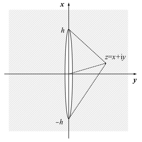
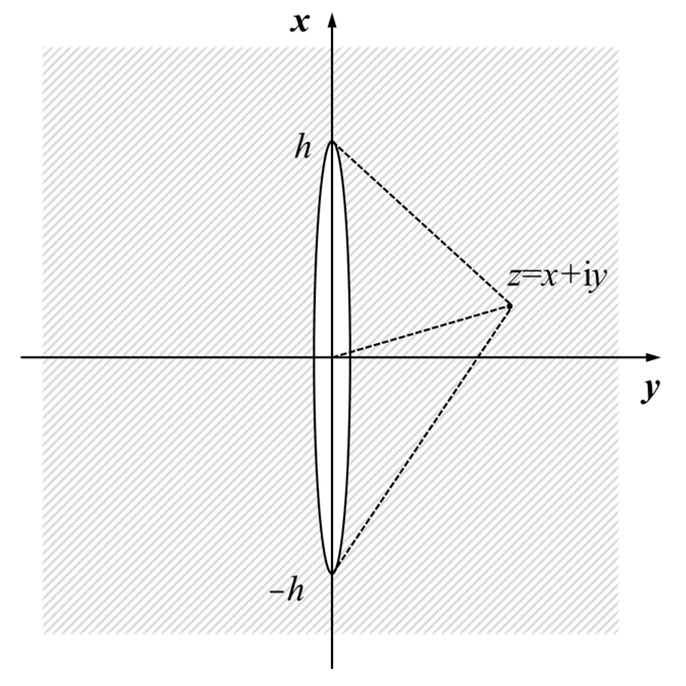
Since the host material strain in the expressions for fiber displacement and strain distribution is unknown, another model is required to determine it. The fiber optic system installed in the fracturing well primarily detects near-wellbore flow and deformation, while far-field fracture deformation has a negligible effect on measurements. The fracture is assumed to be blade-shaped and perpendicular to the fiber, corresponding to Mode I displacement. The single propagating fracture can then be treated as a single infinite-length fracture with constant height along the fracture length, thereby simplifying the computation of the axical strain in the near-wellbore formation from a three-dimensional problem to a half-plane problem. The physical model of this problem is illustrated in Figure 2.

Figure 2. Coordinate system for the Sneddon solution of stress around a semi-infinite fracture.

In Figure 2, y denotes the fiber axial direction, x denotes the fracture height direction, h is the fracture half-height and z represents the coordinate of an arbitrary point in the complex plane. The equilibrium differential equation for this problem is expressed as

$$\left\{\begin{array}{l}{\displaystyle \frac{\partial {\sigma }_x}{\partial x}}+{\displaystyle \frac{\partial {\tau }_{xy}}{\partial y}}=0\\ {\displaystyle \frac{\partial {\tau }_{yx}}{\partial x}}+{\displaystyle \frac{\partial {\sigma }_y}{\partial y}}=0\end{array}\right.$$

(11)

The boundary conditions are given by

$$\left\{\begin{array}{lll}\sigma =0,\hfill & u_x=u_y=0\hfill & (x^2+y^2\to \infty )\hfill \\ {\sigma }_y=-P,\hfill & {\tau }_{xy}=0\hfill & (y=0,\left|x\right|\le h)\hfill \\ u_y=0\hfill & \hfill & (y=0,\left|x\right|>h)\hfill \end{array}\right.$$

(12)

where σ denotes the stress tensor, and σ_x and σ_y are normal stress in the x and y directions. τ_xy is the shear stress. u_x and u_y are displacement in the x and y directions. P is net pressure within the fracture.

Applying the Westergaard stress function method [25,26] to solve the equation gives

$$\left\{\begin{array}{l}{\sigma }_x=\mathrm{Re}Z-y\mathrm{Im}{Z}^{\prime }\hfill \\ {\sigma }_y=\mathrm{Re}Z+y\mathrm{Im}{Z}^{\prime }\hfill \\ {\tau }_{xy}=-y\mathrm{Re}{Z}^{\prime }\hfill \end{array}\right.$$

(13)

where Z is a function of z that satisfies the boundary conditions. $Z^{\prime }$ is the first derivative of Z with respect to z.

In this case, the Westergaard stress function takes the following form [26,27]:

$$Z(z)=P\left[{\displaystyle \frac{z}{\sqrt{z^2-h^2}}}-1\right]$$

(14)

At x = 0, the solution is obtained as

$${\sigma }_x=P\left[{\displaystyle \frac{{\left|y\right|}^3+2h^2\left|y\right|}{{\left(h^2+y^2\right)}^{3/2}}}-1\right]$$

(15)

$${\sigma }_y=P\left[{\displaystyle \frac{{\left|y\right|}^3}{{\left(h^2+y^2\right)}^{3/2}}}-1\right]$$

(16)

According to Hooke’s law for plane strain problems

$${\epsilon }_y={\displaystyle \frac{1+\upsilon }{E}}\left[\left(1-\upsilon \right){\sigma }_y-\upsilon {\sigma }_x\right]$$

(17)

by substituting Equations (15) and (16) into Equation (17), axial strain along the fiber direction in the near-wellbore formation during fracturing is obtained as

$${\epsilon }_{\mathrm{m}}={\epsilon }_y={\displaystyle \frac{P\left(1+\upsilon \right)}{E}}\left[{\displaystyle \frac{\left(1-2\upsilon \right){\left|y\right|}^3-2\upsilon h^2\left|y\right|}{{\left(h^2+y^2\right)}^{3/2}}}+(2\upsilon -1)\right]$$

(18)

where ν is the Poisson’s ratio.

2.2.3. Optical Fiber Strain Model

By differentiating both sides of Equation (18), the relationship between the maximum fracture width and net pressure within the fracture is obtained as

$$u_y={\displaystyle \frac{w}{2}}={\displaystyle \frac{2\left(1-{\nu }^2\right)Ph}{E}}$$

(19)

The fiber displacement is obtained by substituting Equations (18) and (19) into Equation (9)

$$u_{\mathrm{f}}\left(y\right)=\mathrm{sgn}(y)\left\{{\displaystyle \frac{w}{2}}\left(1-e^{-\lambda \left|y\right|}\right)+{\displaystyle \frac{w}{4(1-\upsilon )h}}{\displaystyle \underset{0}{\overset{\left|y\right|}{\int }}\left[\frac{\left(1-2\upsilon \right){\left|y^{\prime }\right|}^3-2\upsilon h^2\left|y^{\prime }\right|}{{\left(h^2+{y^{\prime }}^2\right)}^{3/2}}+(2\upsilon -1)\right]\mathrm{d}{y}^{\prime }}\right\}$$

(20)

The fiber strain is obtained by substituting Equations (18) and (19) into Equation (10), as follows:

$${\epsilon }_{\mathrm{f}}\left(y\right)={\displaystyle \frac{\lambda w}{2}}{e}^{-\lambda \left|y\right|}+{\displaystyle \frac{\left(1-2\upsilon \right){\left|y\right|}^3-2\upsilon h^2\left|y\right|}{{\left(h^2+y^2\right)}^{3/2}}}+(2\upsilon -1)$$

(21)

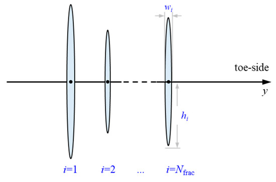
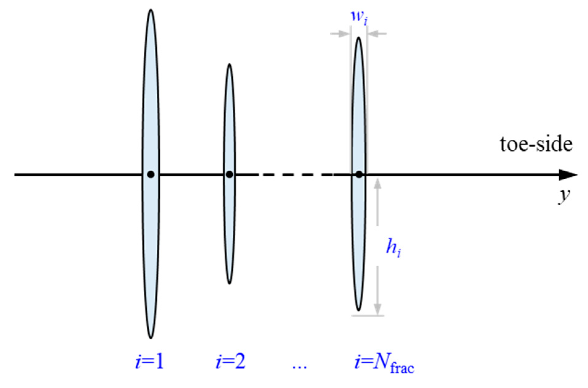
For the case of multi-cluster fracturing, it is assumed that the center of fractures is located at the same depth (Figure 3). Based on the superposition principle, the fiber displacement profile for multi-cluster fracture initiation is given by Equation (22).

$$u_{\mathrm{f}}\left(y\right)={\displaystyle \sum _{i=1}^{N_{\mathrm{frac}}}\mathrm{sgn}(y-y_i)\left\{\frac{w_i}{2}\left(1-e^{-\lambda \left|y-y_i\right|}\right)+\frac{w_i}{4(1-\upsilon )h_i}{\displaystyle \underset{0}{\overset{\left|y-y_i\right|}{\int }}\left[\frac{\left(1-2\upsilon \right){\left|y^{\prime }\right|}^3-2\upsilon {h_i}^2\left|y^{\prime }\right|}{{\left({h_i}^2+{y^{\prime }}^2\right)}^{3/2}}+(2\upsilon -1)\right]\mathrm{d}{y}^{\prime }}\right\}}$$

(22)

Figure 3. Schematic diagram of multi-cluster fracturing.

Field-acquired DAS measurements represent the variation of physical quantities over a distance of gauge length of the fiber, rather than the actual values at the measurement points. This conversion is performed using Equation (23) as follows:

$${\epsilon }_{\mathrm{measure}}\left(y\right)={\displaystyle \frac{u_{\mathrm{f}}\left(y+\frac{L_{\mathrm{G}}}{2}\right)-u_{\mathrm{f}}\left(y-\frac{L_{\mathrm{G}}}{2}\right)}{L_{\mathrm{G}}}}$$

(23)

where ε_measure denotes the strain converted from actual DAS measurements.

2.3. Forward Model Validation

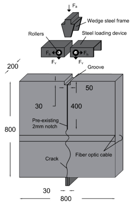
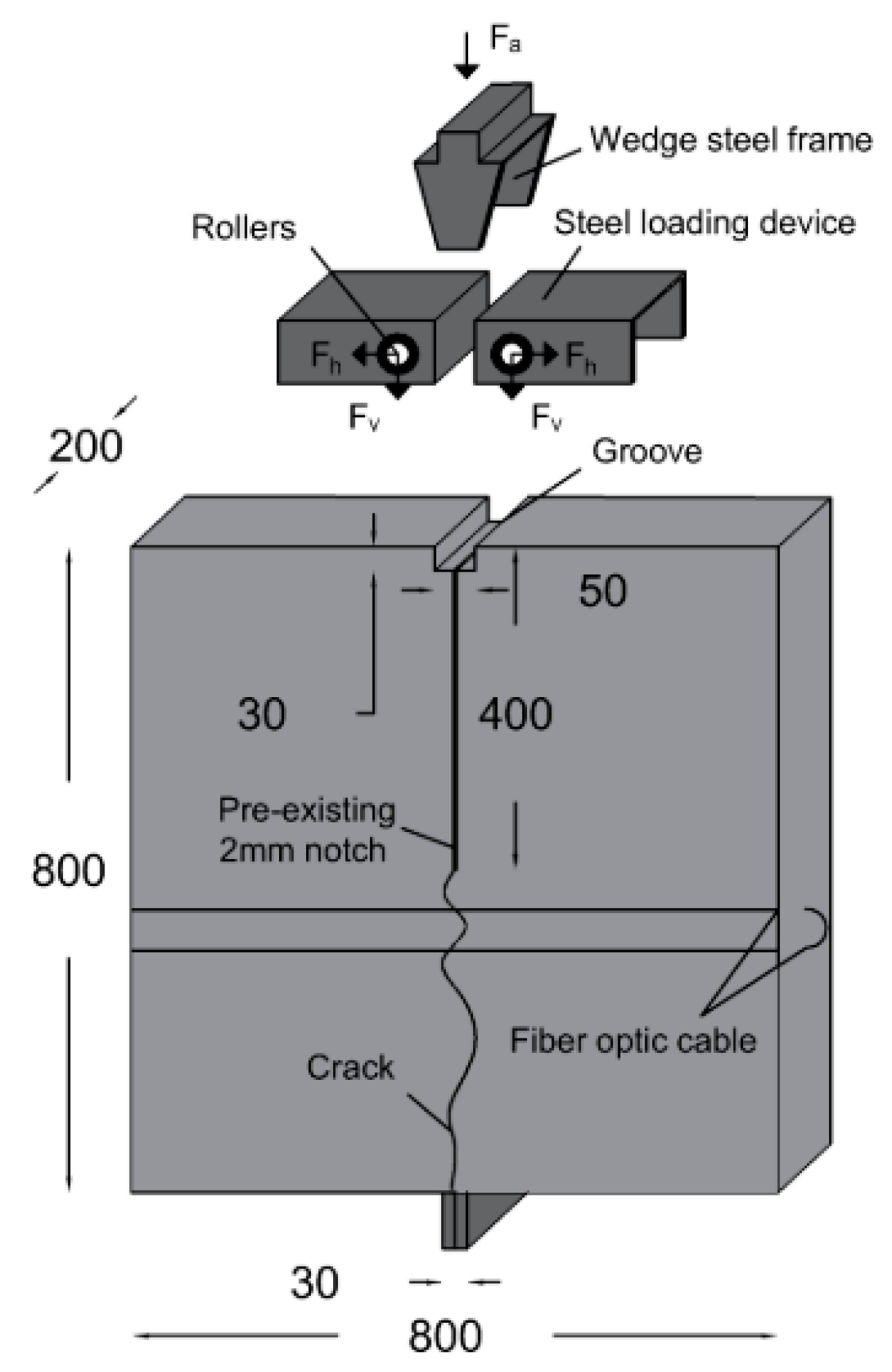
Bassil et al. [24] performed a wedge splitting test (WST) using an optical backscattering reflectometry system and a linear variable differential transformer (LVDT). The fiber strain response and the crack width at the fiber location were measured as the crack propagated towards the metallic support. The schematic of the testing setup is illustrated in Figure 4. The interrogator unit employed in the experiment had a spatial resolution of 1.3 mm. The LVDT had a displacement precision of 1 µm and measurement range of 10 mm.

Figure 4. The schematic of WST [24].

Strain in the host material localized at the crack process zone disappears later in the macrocracking stage. Therefore, strain in the tested concrete specimen could be neglected during the test. Strain in fiber in WST can be expressed as follows:

$${\epsilon }_{\mathrm{f}}\left(y\right)={\displaystyle \frac{\lambda w}{2}}{e}^{-\lambda \left|y\right|}$$

(24)

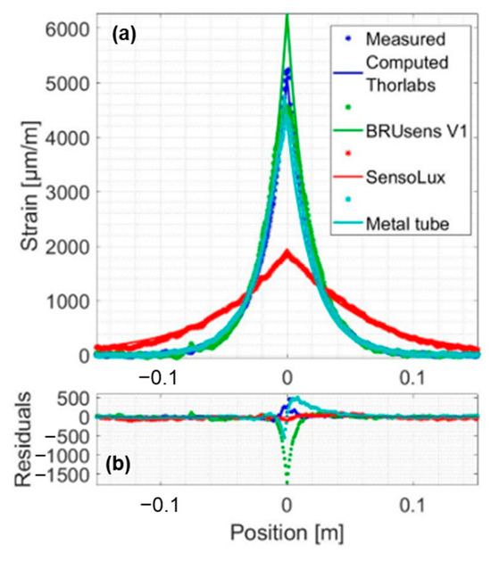
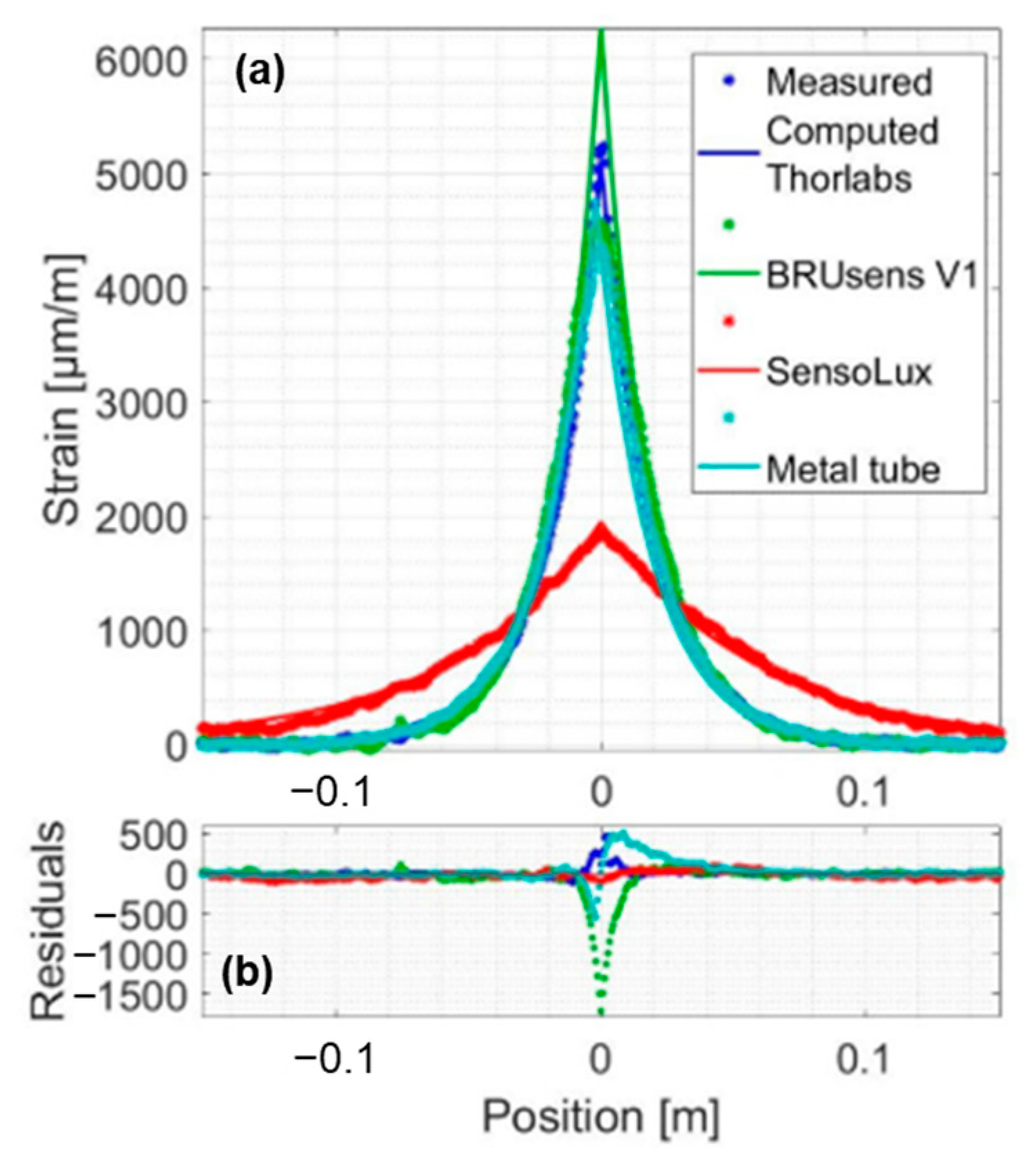
Equation (24) is derived from Equation (10) by neglecting the host material strain term on the right-hand side; thereby only strain resulting from crack width variation was considered in the fiber strain. The analytical results from Equation (24) showed consistency with the measured strain in WST (Figure 5), confirming the reliability of Equation (24). In Figure 5, colors represent the type of optical fibers used in WST. In Figure 5a, the star marker represents the experimental measurement, and the solid line represents the analytical result obtained from Equation (24).

Figure 5. (a,b) Comparison between analytical results and measured strain for a crack width of 200 μm [24].

The host material strain term is non-linear and non-negligible during in-well LF-DAS fracturing monitoring. It is difficult for existing laboratory experiments of fracturing to monitor the formation rock strain and measure the fracture width and height simultaneously. Therefore, numerical simulation is employed to validate the analytical method proposed in this study. Hao et al. [12] extended the traditional PKN model and built a forward model of strain during a single-fracture propagation process based on a semi-analytical finite element method. The model assumes a quasi-static fracture propagation process and incorporates the following assumptions: (a) the fracturing fluid is a Newtonian fluid and full-fills the fracture, (b) the fracturing fluid exhibits laminar flow within the fracture, (c) the formation rock is an impermeable linear-elastic material, (d) the leak-off of the fracturing fluid is neglected.

Host material strain term was calculated by Hao’s model, while the fiber strain resulting from the change in fracture width was calculated via Equation (24). The in-well fiber strain during single fracture propagation was then obtained by summing these two components according to Equation (10). Parameters used in the numerical simulation are listed in Table 1. The analytical method results obtained from Equation (21) were compared with the numerical simulation results to validate the proposed analytical method, since the influence of gauge length on the measurements was not considered in the model validation.

Table 1. Parameters used in the numerical simulation.

Parameter	Value
Young’s modulus, GPa	30
Poisson’s ratio	0.22
Formation density, kg/m3	2560
Pumping rate, m3/min	3
Fracturing fluid viscosity, mPa·s	5
Fracture height, m	20
Fiber lag parameter, m−1	0.05

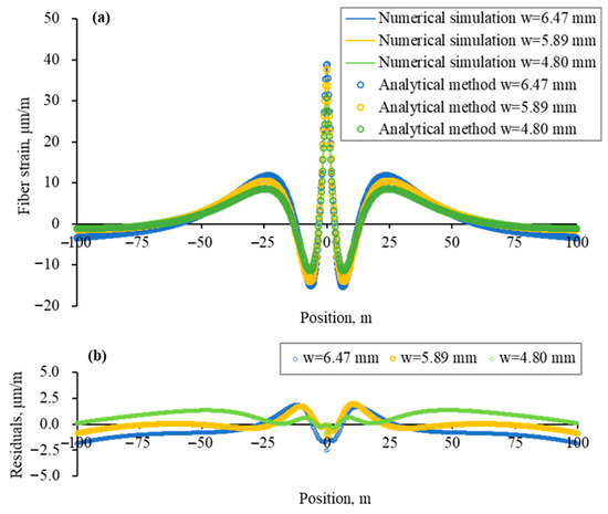
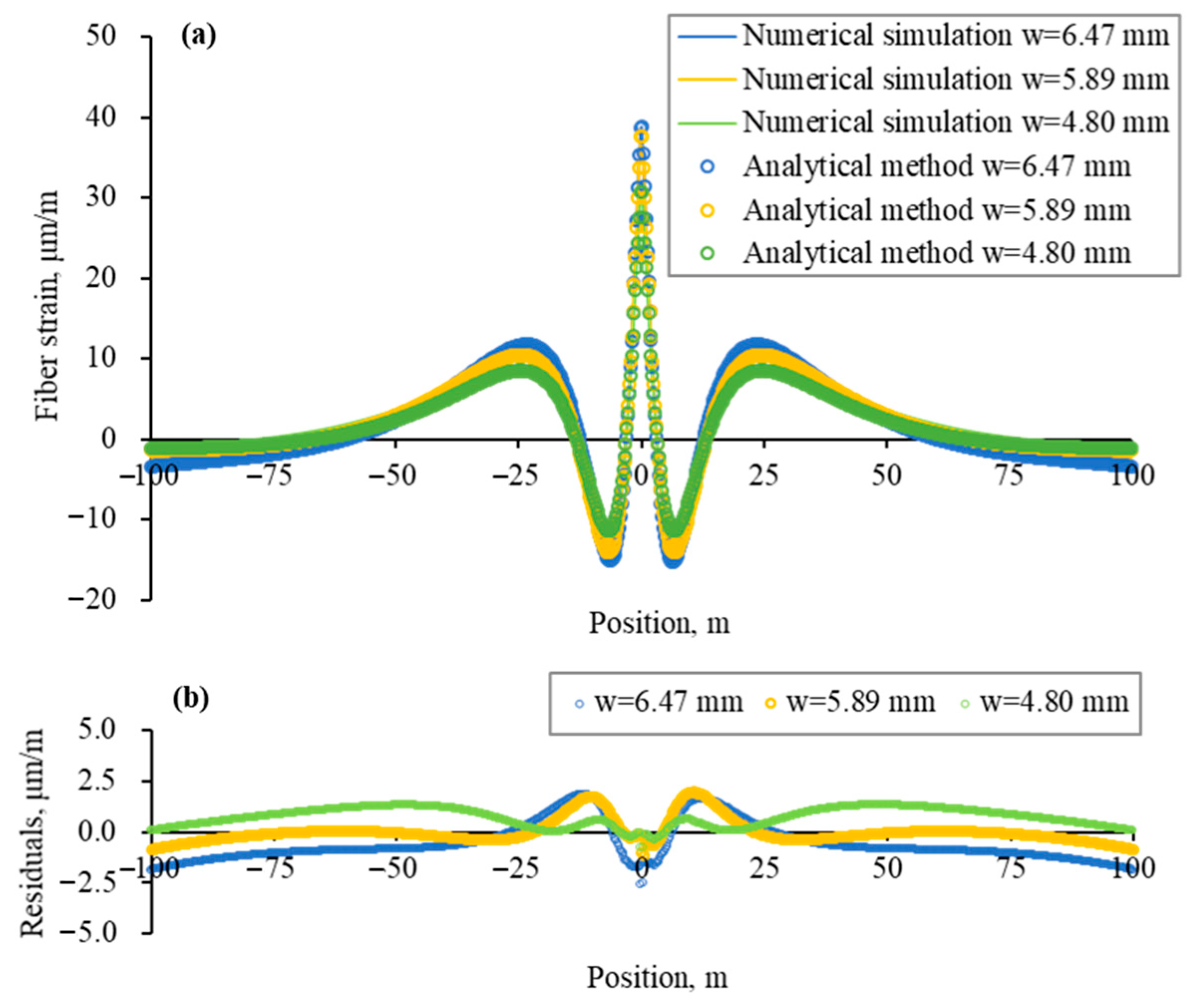
Figure 6a illustrates the comparison between fiber strain profiles calculated by numerical simulation and the analytical method. The fracture was set to initiate at position zero. The residual profile is shown in Figure 6b.

Figure 6. (a) Comparison of strain profiles obtained from numerical simulation and the analytical method; (b) Residuals between numerical simulation results and analytical method results.

In the case of single-fracture propagation, the fiber strain profile is symmetric about the fracture initiation location, and fiber strain reaches a local peak at that point. The stress shadow effect can be observed in the near-fracture region. Fiber strain approaches zero at distances far from the fracture location. Fiber strain derived from the analytical method shows agreement with that from the numerical simulation in both trend and magnitude. Residual at the fracture location is less than 5% of the numerical simulation results.

3. Sensitivity Analysis

Based on the analytical model, mechanical strain measured by the in-well fiber during fracturing was obtained. The effects of fracture size, monitoring parameters, and formation geomechanical parameters on the strain response were analyzed. The analysis considered a single fracture initiating at the zero point and a measurement interval of 0.5 m. The mechanical strain profiles in this section were obtained based on Equations (20) and (23).

3.1. Fracture Size

The model developed for in-well fracturing monitoring is based on the infinite-length fracture assumption, thus is not applicable to analysis of fracture length. Therefore, only the effects of fracture width and height on fiber mechanical strain response were considered in this section. The formation geomechanical parameters and monitoring parameters are listed in Table 2.

Table 2. Geomechanical and monitoring parameters for fracture size sensitivity analysis.

Parameter	Value
Young’s modulus, GPa	30
Poisson’s ratio	0.22
Fiber lag parameter, m−1	0.05
Gauge length, m	1

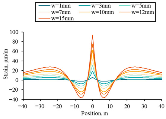
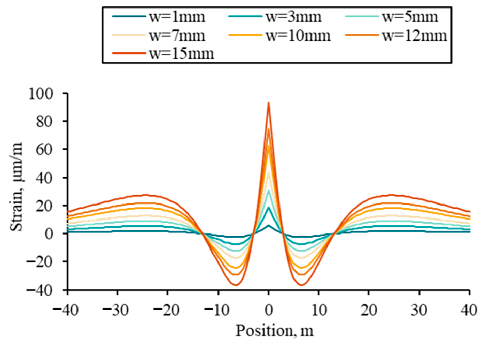
First, the effect of fracture width on fiber strain was analyzed, with the fracture height set at 20 m, while the fracture width was varied across a range of 1–15 mm. Figure 7 shows that fiber strain at the fracture initiation location increases with fracture width, accompanied by an intensified compressive strain in the near-fracture region due to the stress shadow effect. Notably, fracture width has minimal impact on the spatial extent of the stress shadow zone.

Figure 7. Fiber strain profiles under different fracture widths.

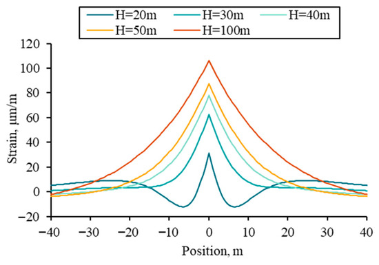
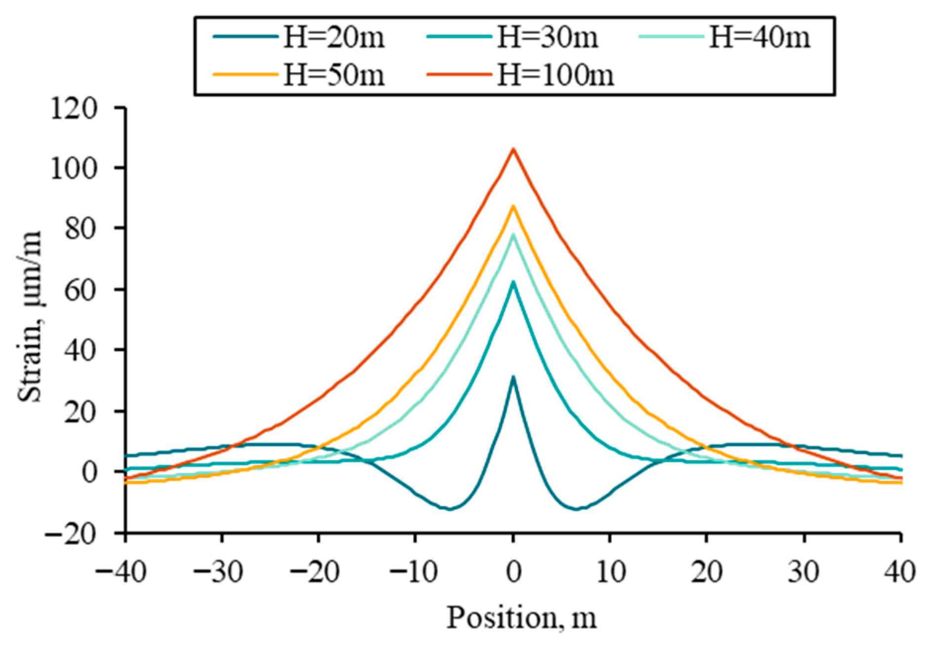
With the fracture width fixed at 5 mm, fiber strain was simulated for fracture heights of 20, 30, 40, 50, and 100 m. The results are presented in Figure 8. Under the same conditions, larger fracture height results in lower net pressure within the fracture, thereby weakening the stress shadow effect on the region adjacent to the fracture. Fiber strain at the fracture location increases as fracture height increases.

Figure 8. Fiber strain profiles under different fracture heights.

3.2. Monitoring Parameters

The sensitivity of fiber-measured strain response to the fiber lag parameter and gauge length is analyzed in this section. The fiber lag parameter is primarily determined by the fiber cable used in field applications, while gauge length is selected based on the range available in the DAS interrogator unit. Other parameters are provided in Table 3.

Table 3. Geomechanical and fracture size parameters for monitoring parameters sensitivity analysis.

Parameter	Value
Young’s modulus, GPa	30
Poisson’s ratio	0.22
Fracture width, mm	5
Fracture height, m	20

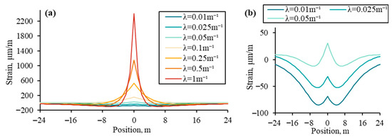
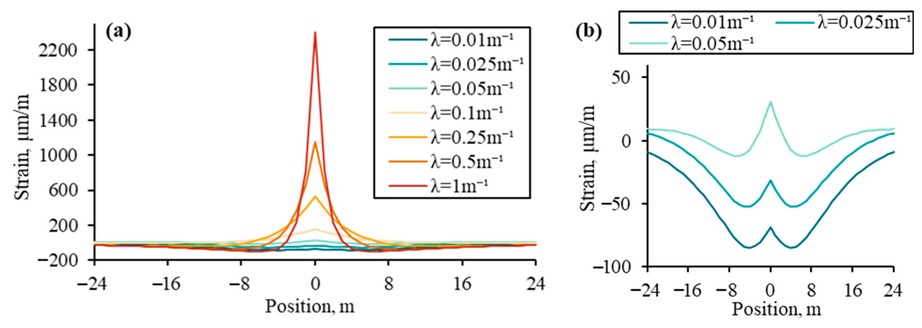
The effect of fiber lag parameter on the fiber strain is investigated with a gauge length of 1 m. Figure 9a shows the fiber strain profiles for different fiber lag parameters, while Figure 9b provides a detailed view of the results in Figure 9a.

Figure 9. (a) Fiber strain profiles under different fiber lag parameters; (b) Partial enlarged view of (a).

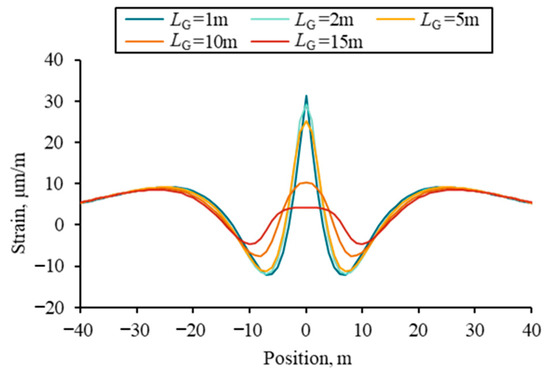
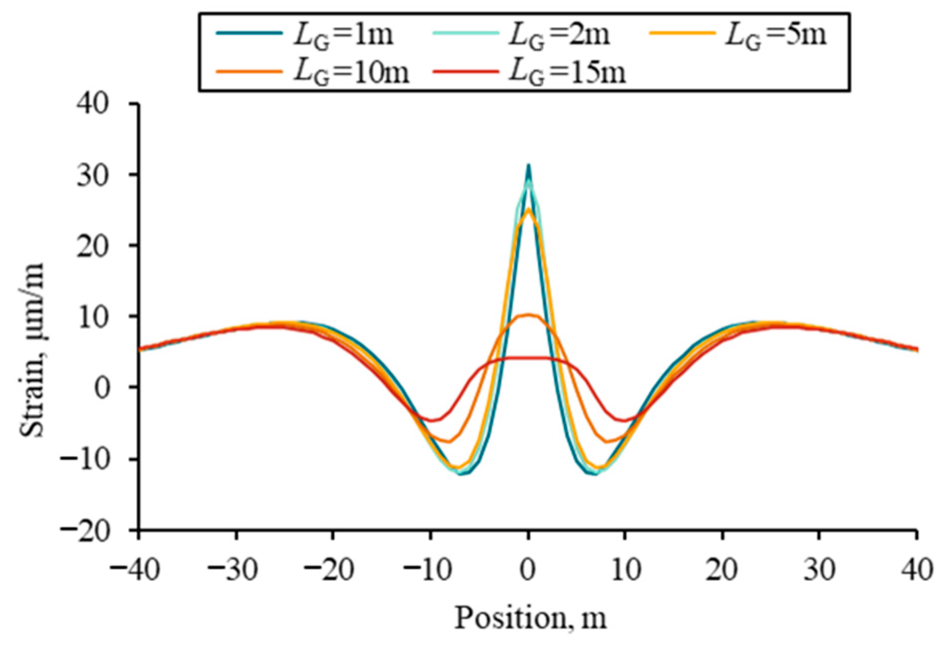
Under the single-fracture propagation condition, the fiber lag parameter influences both peak strain at the fracture location and the overall trend of the fiber strain profile. With a lower fiber lag parameter (Figure 9b), the compressive deformation of the formation near the fracture remains observable. A higher fiber lag parameter results in a pronounced increase in fiber strain at the fracture location, as the tensile strain induced by fracture opening progressively dominates the response. To analyze the effect of gauge length, values of 1, 2, 5, 10, and 15 m were selected, with the fiber lag parameter fixed at 0.05 m⁻¹. Figure 10 illustrates the fiber strain profiles under various gauge lengths.

Figure 10. Fiber strain profiles under different gauge lengths.

As gauge length increases, fiber strain measured at the fracture location diminishes. Additionally, the characteristic local peak in the fiber strain profile becomes increasingly difficult to discern.

3.3. Formation Geomechanical Parameter

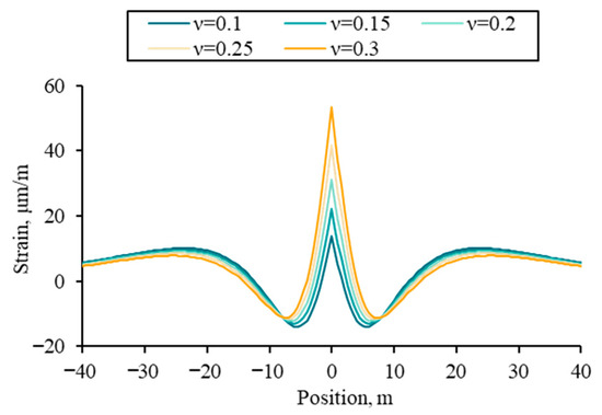
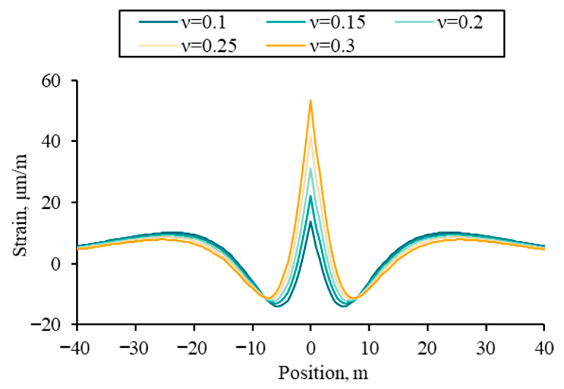
The Sneddon fracture width solution is incorporated into the model development, allowing the effect of formation of Young’s modulus on strain in the near-wellbore formation to be indirectly represented through its impact on fracture width. Consequently, only the effect of Poisson’s ratio on the fiber strain response is analyzed in this section.

Analyses are performed with a fracture width of 5 mm, fracture height of 20 m, fiber lag parameter of 0.05 m⁻¹, and gauge length of 1 m. Fiber strain response was simulated for Poisson’s ratios of 0.1, 0.15, 0.2, 0.25, and 0.3, with the results illustrated in Figure 11. With increasing Poisson’s ratio, fiber strain at the fracture location increases, while the spatial extent of the stress shadow zone near the fracture exhibits only marginal variation.

Figure 11. Fiber strain profiles under different Poisson’s ratios.

4. Inversion Algorithms

A genetic algorithm was applied to fit the mechanical strain profile and to perform an inversion for globally optimal fracture width and height in a fracture stage. Residuals between the forward model results and mechanical strain derived from the LF-DAS/DTS strain-temperature decoupling method were evaluated. The sum of squared residuals was then adopted as the fitness function for the genetic algorithm (Equation (25)). During inversion, the objective was to minimize the sum squared residual

$$f\left(\left[\mathit{w},\mathit{h}\right]\right)={\displaystyle \sum _{i=1}^n{\left({\epsilon }_{\mathrm{M},i}-{\epsilon }_{\mathrm{f},i}\right)}^2}$$

(25)

where w and h denote the one-dimensional arrays of maximum fracture width and half-height for the multi-cluster fractures, respectively. n is the number of data points in the mechanical strain profile.

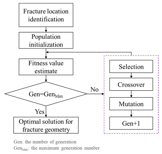
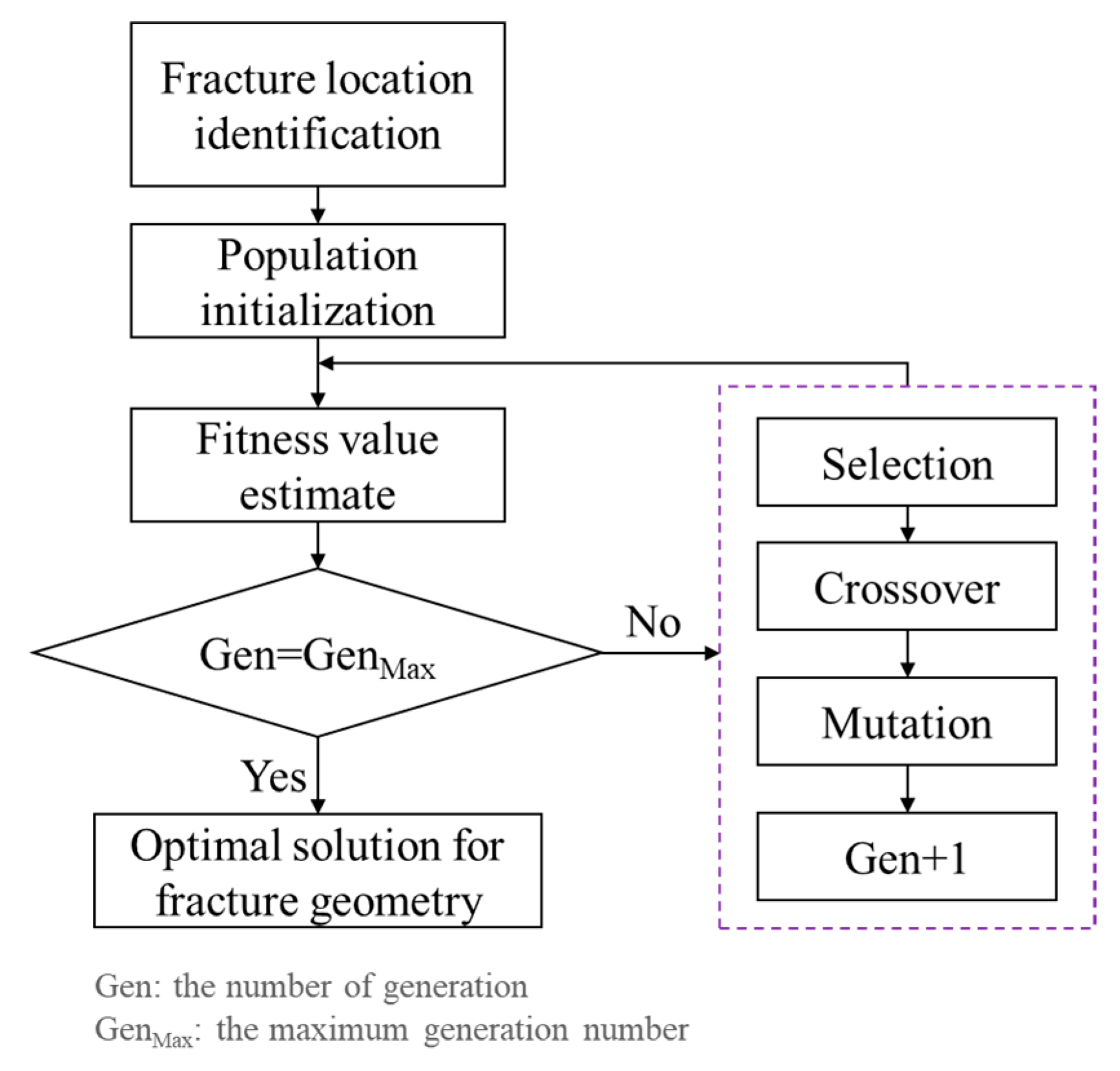
The algorithmic workflow is presented in Figure 12. First, the locations of hydraulic fractures and pre-existing fractures were identified using DAS and LF-DAS monitoring data from the treatment well during fracturing, supplemented by LF-DAS data from adjacent wells when the fracturing well served as a monitoring well. These identified locations were then integrated into the forward model. Subsequently, an initial population representing multi-cluster fracture widths and heights was established. The genetic algorithm then iteratively evolved through steps of fitness evaluation, selection, crossover, and mutation. The optimal solution for fracture width and height was ultimately obtained upon reaching the maximum number of generations and achieving convergence.

Figure 12. Flowchart of the inversion algorithm.

5. Field Application

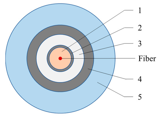
Well A-2 is a multi-stage, multi-cluster fractured horizontal well in a shale reservoir with natural fractures that are poorly developed. Post-fracturing core analysis indicates that the bedding planes within this reservoir had little influence on the hydraulic fracture propagation. DAS and DTS data were measured simultaneously by the fibers installed behind the casing of Well A-2 during the fracturing operation. The structure of the fiber cable is illustrated in Figure 13. Geometrical parameters and size of each protective coating are summarized in Table 4. The shear modulus of Layer 1 is 0.2 × 10⁻⁴ GPa. The fiber diameter is 62.5 μm, with a Young’s modulus of 72 GPa, and a Poisson’s ratio of 0.16. Based on Equation (5), the fiber lag parameter is 0.06 m⁻¹.

Figure 13. The structure of the fiber cable.

Table 4. Parameters of protective coatings.

Layer Index	Diameter mm	Young’s Modulus GPa	Poisson’s Ratio
1	2.10	-	-
2	2.52	195	0.25
3	4.55	68	0.32
4	6.35	195	0.25
5	10.41	1.5	0.42

Well A-1, located on the same pad, was fractured one year prior to the fracturing of Well A-2, at which time the fiber cable had already been installed in Well A-2. The two wells are separated by a distance of 250 m, with parallel horizontal well sections at the same depth. The perforation cluster spacing ranges from 6 to 12 m in both two wells. During monitoring, gauge length was configured to 15 m for cross-well monitoring and 5 m for in-well monitoring. Frac-hit strain responses were identified during the Well A-1 fracturing process by fibers installed in Well A-2. Furthermore, fractures induced during the hydraulic fracturing of Well A-1 were subsequently reactivated during the fracturing operations of Well A-2.

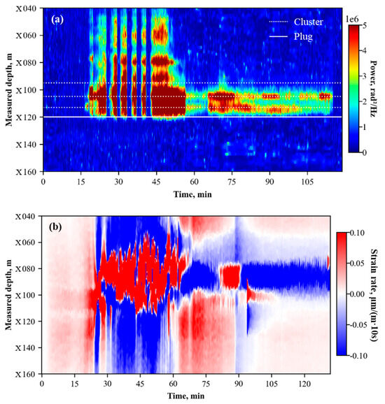
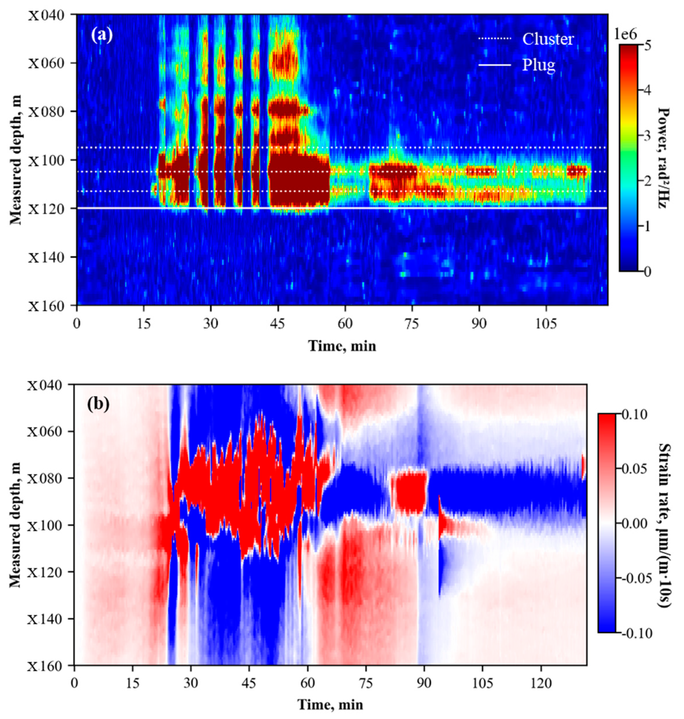
Figure 14 displays waterfall plots from Well A-2 fiber monitoring during the fracturing of Well A-1 and Well A-2, capturing the reactivation of pre-existing fractures. During the fracturing operation of Stage 18 in Well A-1, cross-well LF-DAS captured characteristic heart-shaped strain responses at measured depths of X080 m and X090 m (Figure 14a), indicating the frac-hit locations. The interval between MD X060 m and X110 m was dominated by tensile strain rate responses. Subsequently, during the fracturing of Stage 17 in Well A-2, the in-well waterfall plot (Figure 14b) exhibited pronounced acoustic responses at measured depths of X060 m, X080 m, and X090 m, even though there was no perforation operated in those locations.

Figure 14. Waterfall plots during the fracturing process: (a) Cross-well LF-DAS waterfall plot during Well A-1 Stage 18 fracturing; (b) In-well DAS waterfall plot during Well A-2 Stage 17 fracturing.

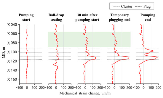
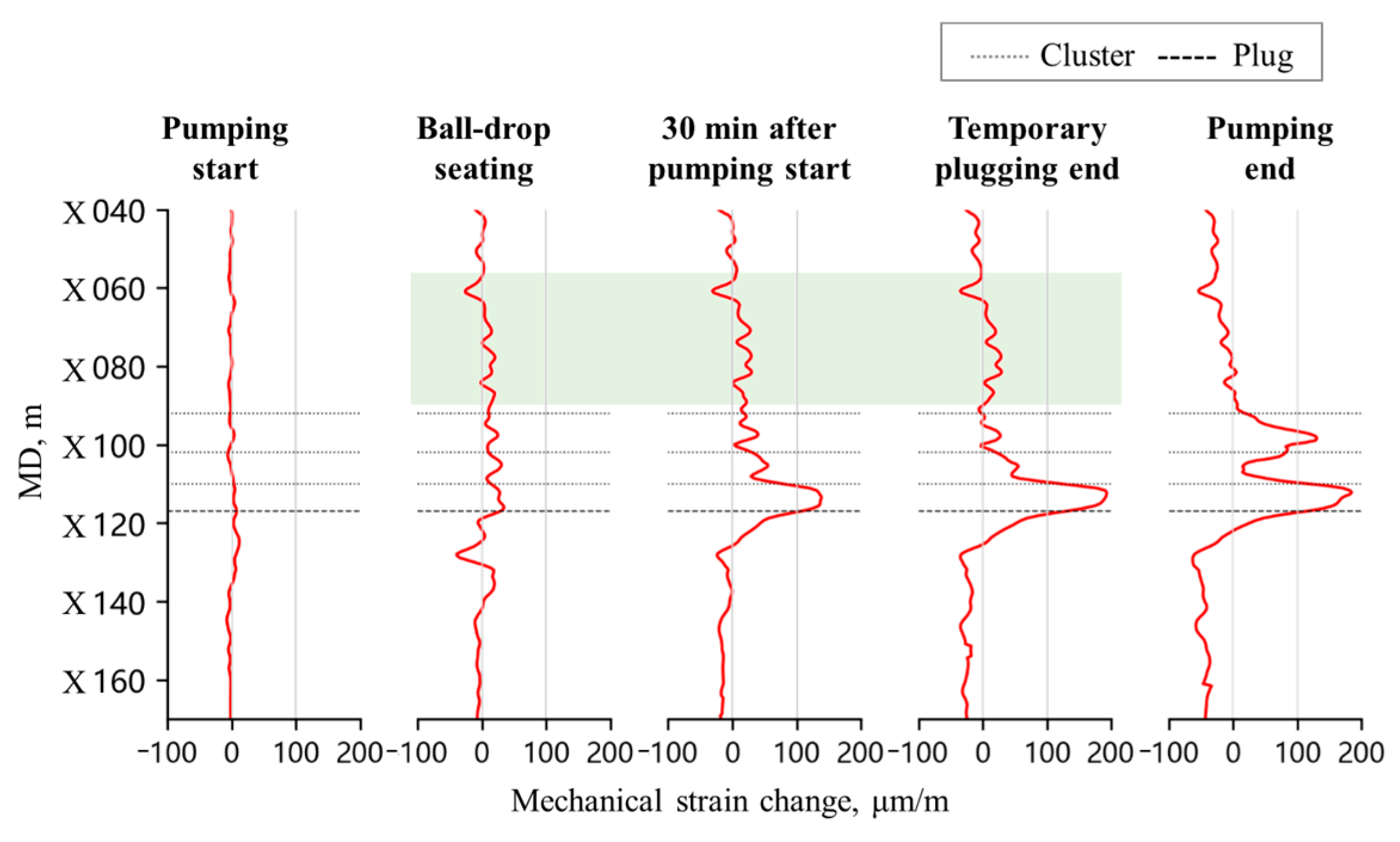
Figure 15 is the timing-slicing plots of mechanical strain profile for Stage 17 of Well A-2. The non-perforated intervals that displayed acoustic responses during fracturing also exhibited significant tensile strain responses (indicated by the green highlighted area in Figure 15). These phenomena indicate that during Well A-2 fracturing, the fracturing fluid entered both newly initiated hydraulic fractures via perforation clusters and pre-existing fractures through the near-wellbore region, thereby resulting in reactivation of the latter.

Figure 15. Timing-slicing plots of mechanical strain profile at Stage 17 of Well A-2.

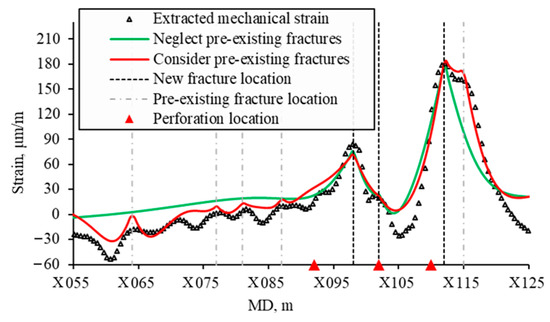
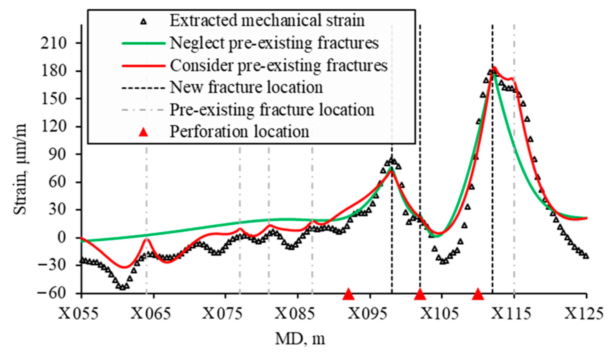
Two fitting cases were performed to fit the mechanical strain profile at the pumping end time of the Stage 17 fracturing: one accounted for the influence of pre-existing fractures and the other neglected it. In the case accounted for pre-existing fractures, potential variation in the geomechanical parameter of the reservoir were not taken into consideration. Fitting results are shown in Figure 16. The fitted curves are consistent with the overall trend of the mechanical strain profile, demonstrating good fitting performance.

Figure 16. Fitted mechanical strain profiles at Stage 17 of Well A-2.

Based on a comprehensive analysis of cross-well LF-DAS data from Well A-1 and in-well DAS/DTS monitoring results, three newly initiated hydraulic fractures and five reactivated fractures were identified at the end of pumping. The initiation locations of new fractures did not strictly coincide with perforation positions but exhibited a discernible spatial offset. The reactivated pre-existing fractures were located at measured depths of X059 m, X072 m, X076 m, X082 m, and X110 m. These fractures comprised fractures propagated during the fracturing of Well A-1, as well as a fracture initiated during the Stage 16 fracturing of Well A-2 (at MD X110 m). The inversed new fracture widths and heights are listed in Table 5.

Table 5. The inversed new fracture width and height in two fitting cases.

MD m	Neglect Pre-Existing Fractures		Account for Pre-Existing Fractures
	Fracture Width mm	Fracture Height m	Fracture Width mm	Fracture Height m
X098	6.86	21.78	4.35	19.5
X102	1.39	9.84	0.50	9.82
X112	12.35	23.52	10.51	20.74

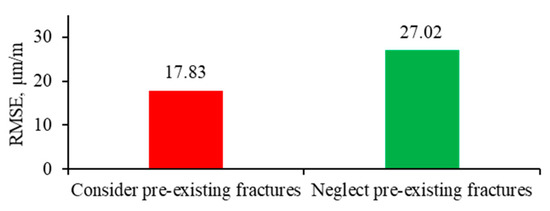
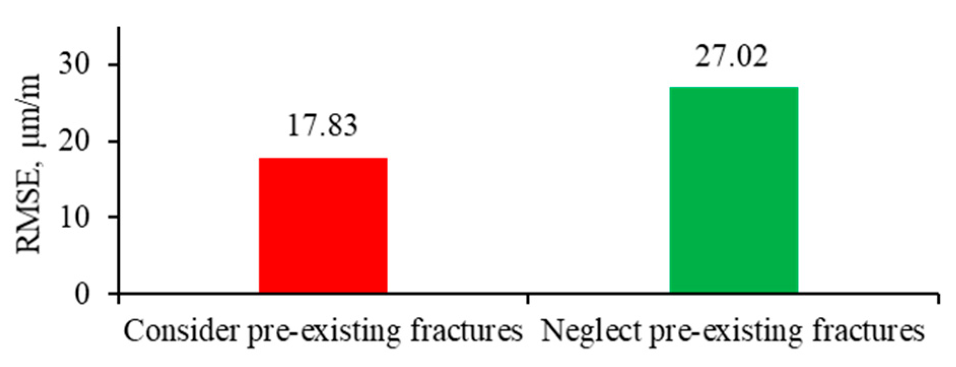
Inversed fracture width and height were larger when pre-existing fractures were neglected. Accounting for pre-existing fractures yielded better fitting results than neglecting them, as evidenced by a root mean square error (RMSE) that was 1.51 times higher when pre-existing fractures were not considered (Figure 17).

Figure 17. Bar chart of the RMSE for the two fitting cases.

6. Method and Study Limitations

The analytical method simplifies single fracture propagation to the opening of a semi-infinite fracture with a constant height in the formation strain model. Furthermore, the model relies on several fundamental assumptions, including that the formation is homogeneous and isotropic linear elastic material. The proposed method is applicable to scenarios where vertical fractures propagate during horizontal well fracturing. While it effectively characterizes near-wellbore fracture geometry, it cannot capture far-field features, such as fracture length. In more complex cases, such as inclined fractures or the reactivation of bedding planes, alternative models must be employed to compute formation strain.

The proposed method assumes perfect bonding between the fiber optic cable, cement sheath, and formation. Consequently, calculation of the fiber lag parameter does not account for decoupling between the fiber and its protective coatings. A theoretical framework for calculating fiber lag parameter under imperfect bonding conditions can be found in Ref. [23]. As fiber lag parameter is a critical factor influencing analytical method results, experimental calibration of the actual parameter is advisable prior to optical fiber cable deployment.

7. Conclusions

This study developed an analytical method based on strain transfer theory to interpret fiber strain profiles measured by in-well fiber during fracturing. The proposed method facilitates the identification of hydraulic fracture and pre-existing fracture reactivation location, as well as the inversion of fracture width and height. The reliability of the analytical method was validated through numerical simulation of the three-dimensional formation strain field during single-fracture propagation.

Under the single-fracture propagation condition, the in-well fiber strain profile exhibits a localized peak at the fracture location. The peak magnitude of the fiber strain correlates positively with increases in fracture width and height. Tensile deformation induced by fracture opening plays a pivotal role in fiber strain response. However, compressive deformation near the fracture remains discernible in the fiber strain profile under conditions of low fiber lag parameter.

The proposed analytical method was applied to interpret the mechanical strain profile extracted from in-well LF-DAS/DTS measurements. Fracture width and height at the end of pumping for a fracturing stage were inversed. Due to early installation of the optical fiber system, fractures induced by the adjacent well were captured prior to the stimulation of the fiber-installed well. By considering the reactivation of these pre-existing fractures into the inversion process, a better match with the extracted mechanical strain profile was achieved.

References

- Ugueto, G.A.; Todea, F.; Daredia, T.; Wojtaszek, M.; Huckabee, P.T.; Reynolds, A.; Laing, C.; Chavarria, J.A. Can You Feel the Strain? DAS Strain Fronts for Fracture Geometry in the BC Montney, Groundbirch. In Proceedings of the SPE Annual Technical Conference and Exhibition, Calgary, AB, Canada, 30 September–2 October 2019. [Google Scholar]
- Ciezobka, J. Overview of Hydraulic Fracturing Test Site 2 in the Permian Delaware Basin (HFTS-2). In Proceedings of the 9th Unconventional Resources Technology Conference, Houston, TX, USA, 26–28 July 2021. [Google Scholar]
- Qi, Y.; Zhang, T.; Chen, Q.; Ma, B.; Bai, J.; Ye, K.; Tang, J. What Low Frequency Distributed Acoustic Sensing Revealed of The Hydraulic Fracturing in Tight Oil Reservoir: Ordos Case Study. In Proceedings of the International Petroleum Technology Conference, Dhahran, Saudi Arabia, 12–14 February 2024. [Google Scholar]
- Kerr, E.; Barree, R.; Estrada, E. What Can You Learn from a DFIT on Fiber Optics? In Proceedings of the SPE Hydraulic Fracturing Technology Conference and Exhibition, The Woodlands, TX, USA, 6–8 February 2024. [Google Scholar]
- Saw, J.; Zhu, X.; Luo, L.; Correa, J.; Soga, K.; Ajo-Franklin, J. Distributed Fiber Optic Sensing for in-well hydraulic fracture monitoring. Geoenergy Sci. Eng. 2025, 250, 213792. [Google Scholar] [CrossRef] [Scilit]
- Zhang, Z.; Fang, Z.; Stefani, J.; DiSiena, J.; Bevc, D.; Ning, I.L.C.; Hughes, K.; Tan, Y. Fiber Optic Strain Monitoring of Hydraulic Stimulation: Geomechanical Modeling and Sensitivity Analysis. In Proceedings of the SPE/AAPG/SEG Unconventional Resources Technology Conference, Austin, TX, USA, 20–22 July 2020. [Google Scholar]
- Wang, J.; Tan, Y.; Rijken, P.; Liu, X.; Singh, A.; Li, Y. Observations and Modeling of Fiber-Optics Strain on Hydraulic Fracture Height Growth in HFTS-2. In Proceedings of the SPE/AAPG/SEG Unconventional Resources Technology Conference, Houston, TX, USA, 26–28 July 2021. [Google Scholar]
- Liu, Y.; Wu, K.; Jin, G.; Moridis, G. Rock Deformation and Strain-Rate Characterization during Hydraulic Fracturing Treatments: Insights for Interpretation of Low-Frequency Distributed Acoustic-Sensing Signals. SPE J. 2020, 25, 2251–2264. [Google Scholar] [CrossRef] [Scilit]
- Wu, K.; Liu, Y.; Jin, G.; Moridis, G. Fracture Hits and Hydraulic-Fracture Geometry Characterization Using Low-Frequency Distributed Acoustic Sensing Strain Data. J. Pet. Technol. 2021, 73, 39–42. [Google Scholar] [CrossRef] [Scilit]
- Liu, Y.; Jin, G.; Wu, K.; Moridis, G. Hydraulic-Fracture-Width Inversion Using Low-Frequency Distributed-Acoustic-Sensing Strain Data—Part I: Algorithm and Sensitivity Analysis. SPE J. 2021, 26, 359–371. [Google Scholar] [CrossRef] [Scilit]
- Liu, Q.; Ou, Y.; Sharma, M. Factors Controlling the Properties of Hydraulic Fracture Networks in Naturally Fractured Formations. In Proceedings of the SPE Annual Technical Conference and Exhibition, New Orleans, LA, USA, 23–25 September 2024. [Google Scholar]
- Hao, Y.; Chen, M.; Wang, S. Research on the mechanism of LF-DAS fiber-optic strain rate evolution and automatic interpretation method for multivariate monitoring wells. Eng. Fract. Mech. 2025, 322, 111178. [Google Scholar] [CrossRef] [Scilit]
- Srinivasan, A.; Jurick, D.; Haustvei, K.; Jin, G.; Guzik, A.; Wu, K. In-Well Stress Shadow and Near-Wellbore Fracture Geometry Diagnosis Using High-Resolution Distributed Strain Sensing via Rayleigh Frequency Shift. In Proceedings of the Unconventional Resources Technology Conference, Denver, CO, USA, 13–15 June 2023. [Google Scholar]
- Wang, H.; Xiang, P.; Jiang, L. Strain transfer theory of industrialized optical fiber-based sensors in civil engineering: A review on measurement accuracy, design and calibration. Sens. Actuators A Phys. 2019, 285, 414–426. [Google Scholar] [CrossRef] [Scilit]
- Nwabueze, Q.A.; Leggett, S. Proppant consolidation and hysteresis in hydraulic fractures: Insights from the application of a strain transfer model for interpreting fracture width changes from distributed fiber optic strain sensing. Geoenergy Sci. Eng. 2026, 256, 214159. [Google Scholar] [CrossRef] [Scilit]
- Nwabueze, Q.A.; Leggett, S. Physics-Based Interpretation of RFS-DSS for Far-Field Monitoring of Fracture Conductivity. In Proceedings of the SPE Hydraulic Fracturing Technology Conference and Exhibition, The Woodlands, TX, USA, 3–5 February 2026. [Google Scholar]
- Zhang, X.; Guo, Y.; Bi, Z.; Guo, W.; Teng, S. Dynamic Analysis of Hydraulic Fracture Propagation in Indoor Layered Rocks Based on OFDR Technology. Rock Mech. Rock Eng. 2025. [Google Scholar] [CrossRef] [Scilit]
- Song, J.; Sui, W.; Guo, H.; Li, J. Near-Wellbore Fracture Diagnosis via Strain Decoupling from Integrated In-Well LF-DAS and DTS Data. Sensors 2026, 26, 1813. [Google Scholar] [CrossRef] [Scilit] [PubMed]
- Lindsey, N.J.; Rademacher, H.; Ajo-Franklin, J.B. On the Broadband Instrument Response of Fiber-Optic DAS Arrays. J. Geophys. Res. Solid Earth 2020, 125, e2019JB018145. [Google Scholar] [CrossRef] [Scilit]
- Weber, M.; Weatherly, D.; Mahue, V.; Hull, R.A.; Trujillo, K.; Bohn, R.; Jimenez, E. Optimizing Completion Designs for the East Texas Haynesville Utilizing Production Flow Allocations from Lower-Cost Fiber Optic Sensing DAS/DTS Systems. In Proceedings of the SPE/AAPG/SEG Unconventional Resources Technology Conference, Houston, TX, USA, 26–28 July 2021. [Google Scholar]
- Budiansky, B.; Drucker, D.; Kino, G.; Rice, J. Pressure sensitivity of a clad optical fiber. Appl. Opt. 1979, 18, 4085–4088. [Google Scholar] [CrossRef] [Scilit] [PubMed]
- Fang, Z.; Chin, K.K.; Qu, R.; Cai, H. Fundamentals of Optical Fiber Sensors; John Wiley & Sons: New York, NY, USA, 2012. [Google Scholar]
- Feng, X.; Zhou, J.; Sun, C.; Zhang, X.; Ansari, F. Theoretical and Experimental Investigations into Crack Detection with BOTDR Distributed Fiber Optic Sensors. J. Eng. Mech. 2013, 139, 1797–1807. [Google Scholar] [CrossRef] [Scilit]
- Bassil, A.; Chapeleau, X.; Leduc, D.; Abraham, O. Concrete Crack Monitoring Using a Novel Strain Transfer Model for Distributed Fiber Optics Sensors. Sensors 2020, 20, 2220. [Google Scholar] [CrossRef] [Scilit] [PubMed]
- Westergaard, H.M. Bearing Pressures and Cracks. J. Appl. Mech. 1939, 6, A49–A53. [Google Scholar] [CrossRef] [Scilit]
- Sneddon, I.N.; Lowengrub, M. Crack Problems in the Classical Theory of Elasticity; John Wiley & Sons, Inc.: New York, NY, USA, 1969. [Google Scholar]
- Tada, H.; Paris, P.C.; Irwin, G.R. The Stress Analysis of Cracks Handbook, 3rd ed.; ASME Press: New York, NY, USA, 2000. [Google Scholar]
Disclaimer/Publisher’s Note: The statements, opinions and data contained in all publications are solely those of the individual author(s) and contributor(s) and not of MDPI and/or the editor(s). MDPI and/or the editor(s) disclaim responsibility for any injury to people or property resulting from any ideas, methods, instructions or products referred to in the content. |
© 2026 by the authors. Licensee MDPI, Basel, Switzerland. This article is an open access article distributed under the terms and conditions of the Creative Commons Attribution (CC BY) license.