Impact of Hyperparameters on Surrogate Model Performance: Calcite Dissolution Under Geological Disposal Conditions

Abstract

Efficient simulation of geochemical reactions is critical for predicting the long-term chemical evolution of geological disposal repositories for radioactive waste. In large-scale reactive transport simulations, geochemical equilibrium calculations often represent a major computational bottleneck because they must be repeatedly solved for many spatial cells and time steps. This study investigates the development of machine-learning-based surrogate models that are designed to approximate geochemical equilibrium calculations and thereby significantly accelerate reactive transport simulations while reducing computational resource requirements. Calcite dissolution induced by magnesium-rich fluid inflow is used as a representative test case to evaluate the feasibility and performance of such surrogate models. Training and validation datasets were generated using the IPhreeqc C++ API, enabling the automated execution of a large number of PHREEQC equilibrium simulations across a chemically relevant parameter space. The resulting dataset captures nonlinear relationships between initial aqueous composition and outputs of interest after chemical equilibration, including aqueous species concentrations and amounts of minerals. Fully connected feed-forward neural networks were designed and implemented in TensorFlow to reproduce PHREEQC results, and the influence of key hyperparameters—such as network depth, width, activation functions, learning rate, and batch size—was systematically investigated. The results demonstrate that surrogate model accuracy and training stability are sensitive to hyperparameter selection, even for a relatively simple chemical system. Properly configured neural network architectures reproduce equilibrium geochemical responses with high accuracy and provide a computationally efficient alternative to repeated PHREEQC calculations, highlighting their potential for accelerating large-scale reactive transport modelling workflows.

1. Introduction

Nuclear energy remains a key component of global strategies aimed at achieving low-carbon electricity production while enhancing energy security. The operation of nuclear facilities, however, inevitably generates high-level radioactive waste. Geological disposal in deep, stable host formations is internationally recognised as the most viable solution for ensuring the long-term isolation of such waste from the biosphere [1]. Among the relevant aspects for safety assessments of Deep Geological Repositories (DGRs) is the reliable prediction of geochemical processes controlling radionuclide mobility over timescales of thousands to hundreds of thousands of years [2].

The safety of geological disposal facilities for highly radioactive waste is governed by a number of coupled hydraulic, mechanical, thermal, chemical processes taking place in repository engineered and geological barriers that affect radionuclide release and transport if any occurs. As mentioned above, radionuclide transport analysis needs to be performed for timeframes of thousands of years. Therefore, it is a computationally very demanding task. Among other factors, radionuclide mobility and retention in the engineered and geological barriers will highly depend on the prevailing chemical conditions in the porewater. These conditions will be determined by various processes, such as speciation, mineral dissolution/precipitation, ion exchange, surface complexation, etc.

The most common approach used in modern reactive transport simulators is operator splitting of reactions and transport terms, usually in a sequential manner [3]. Often, transport simulations are solved by one computational code while the chemical reactions are handled by a separate geochemical solver [4]. Consequently, information on state variables must be exchanged between the codes at every time step for each spatial node (e.g., iCP [5], HPx [6], PHT3D [7]). In addition, the initialization and execution of the chemical solver (e.g., PHREEQC [8]) for each reaction calculation introduces further computational overhead, resulting in significant computational demands for large-scale systems such as deep geological repositories. Precise and well-trained DNN-based surrogate models significantly reduce these efforts for large-scale reactive transport analysis [9].

Geochemical modelling is essential for understanding mineral–water interactions that control porewater chemistry and mineral formation in geological disposal systems. In such repositories, engineered barriers and surrounding host rocks are continuously exposed to groundwater over long timescales. Under such conditions, calcium-bearing minerals such as calcite may dissolve if the infiltrating water is chemically undersaturated. This process becomes particularly relevant when magnesium-rich fluids interact with cement-based engineered barriers. Calcite dissolution, potentially coupled with dolomite precipitation, alters calcium availability, carbonate speciation, and pH, thereby influencing long-term barrier performance and radionuclide retention. Because these reactions are nonlinear and thermodynamically coupled, their simulation using conventional geochemical solvers can become computationally demanding in large-scale reactive transport analyses.

To address this challenge, this study investigates the use of data-driven surrogate models to approximate geochemical reaction calculations with high accuracy and substantially reduced computational cost. The IPhreeqc [8] application programming interface (API) for C++ is used in an offline workflow to generate comprehensive training and validation datasets. These datasets span a wide range of relevant geochemical states and reaction conditions, capturing the evolution of aqueous species concentrations, mineral saturations, and reaction progress during calcite dissolution and transient dolomite precipitation induced by magnesium inflow.

Several fully connected feed-forward neural networks with varying architectures and algorithms are trained using TensorFlow. A consistent training strategy is applied across all models, including normalisation of input variables, monitoring of convergence behaviour, and the use of independent validation datasets to prevent overfitting. The surrogate models are evaluated against the results obtained from PHREEQC simulations, demonstrating their ability to reproduce key geochemical outputs with high accuracy across the tested parameter space.

2. Methodology

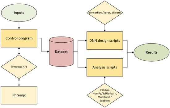
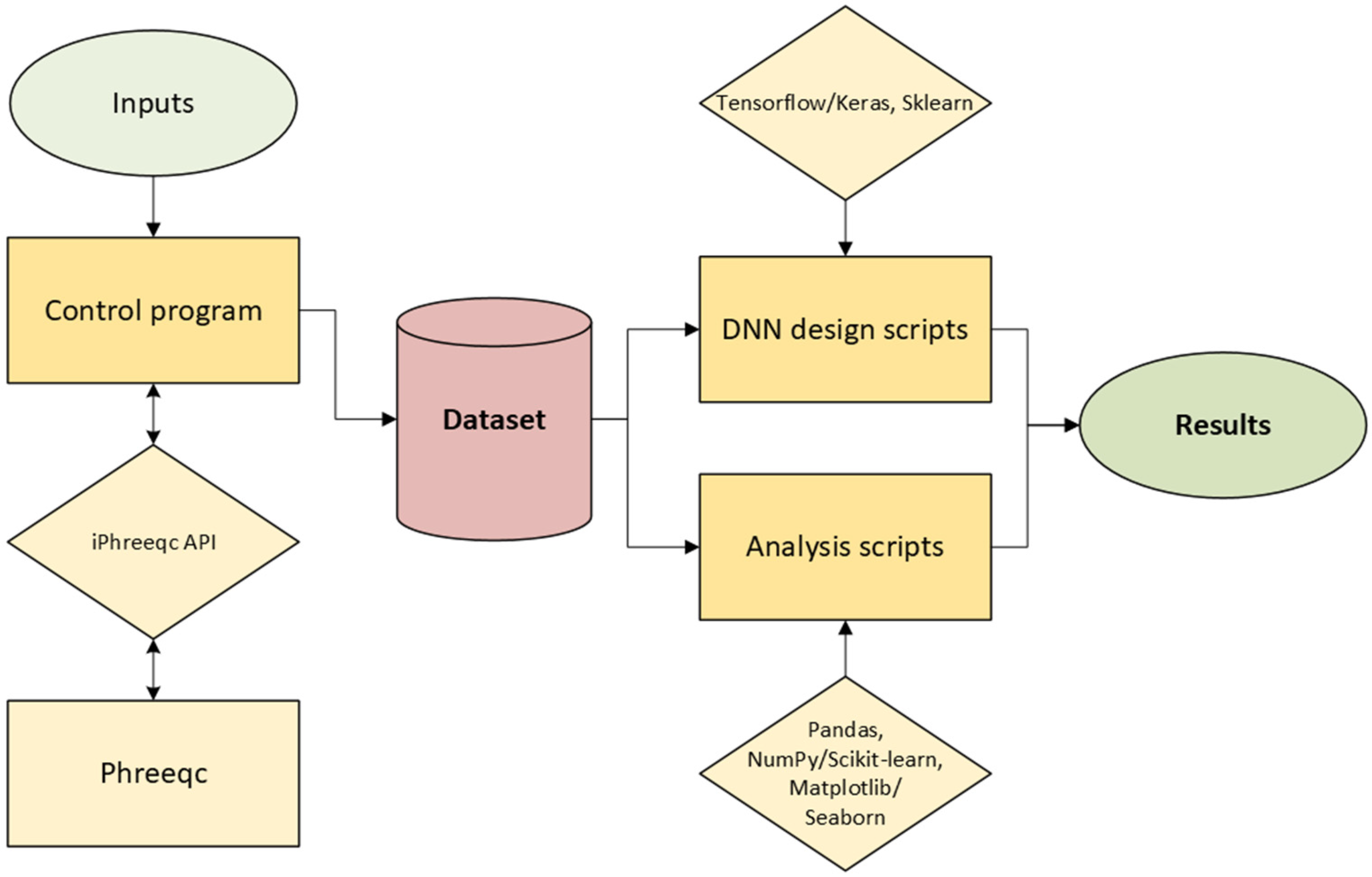
The objective of this work is to effectively approximate the response of purely geochemical calculations using differently tuned surrogate models. The development of a reliable surrogate model requires a carefully designed workflow, in which the generation of high-quality training and validation datasets represents a critical step. The principal schematic of this workflow is shown in Figure 1.

Figure 1. Workflow for surrogate modelling of calcite dissolution using PHREEQC and deep neural networks.

The workflow begins with the definition of input parameters (features, ranges, etc.), which are processed by a control program that interfaces with PHREEQC (Version 3.8.7) through the IPhreeqc API to perform geochemical calculations. These simulations generate a comprehensive dataset representing the system response over a specified range of conditions. The dataset is subsequently used for two distinct purposes. First, it is used in DNN design scripts, where deep neural network (DNN) models are constructed and trained to approximate the geochemical response of the system. These scripts define the model architecture, training process, and optimisation (e.g., using TensorFlow [10]/Keras [11] and scikit-learn [12]). Second, the dataset is used in analysis scripts, which do not build models but instead process and evaluate data. These scripts are used to explore relationships in the dataset, assess model accuracy, and visualise results (e.g., using Pandas [13], NumPy [14], Matplotlib [15], and Seaborn [16]). The trained models and their performance assessment constitute the final results.

2.1. Chemical System Simulated

Calcite dissolution is highly relevant in geological disposal systems that employ cement-based engineered barriers. Cementitious materials contain significant amounts of calcium-bearing phases, including portlandite and calcite, which provide an alkaline buffering environment; calcite is also commonly present in clay-based materials such as bentonite. When external groundwater interacts with these materials, mineral–water reactions govern the long-term chemical evolution of the barrier. If the infiltrating groundwater is undersaturated with respect to calcite, dissolution occurs and releases Ca²⁺ and carbonate species into solution. Over time, this leads to decalcification, potential porosity changes, and modification of the mineral assemblage. In magnesium-rich environments, secondary reactions such as dolomite formation may additionally influence mineral stability and buffering capacity.

In this study, the system to be analysed considers the equilibrium reaction between mineral calcite (CaCO₃) and water containing dissolved MgCl₂. All simulations are restricted to chemical equilibrium reactions and are performed using PHREEQC through the IPhreeqc interface using a PHREEQC-formatted version of the Nagra/PSI Chemical Thermodynamic Database [17], developed for the geochemical modelling of radioactive waste disposal systems. Calcite dissolution is governed by its saturation state, defined by the ion activity product of Ca²⁺ and CO₃²⁻ relative to the mineral solubility product. When the solution is undersaturated (SI < 0), the reaction $\mathrm{C}\mathrm{a}\mathrm{C}{\mathrm{O}}_3(\mathrm{s})\rightleftharpoons \mathrm{C}{\mathrm{a}}^{2+}+\mathrm{C}{\mathrm{O}}_3^{2-}$ proceeds toward dissolution until equilibrium is reached [18]. The dissolved carbonate species further redistribute according to pH-dependent equilibria, forming bicarbonate and carbonic acid species, which directly affect solution pH and buffering behaviour [18].

The presence of Mg²⁺ modifies the equilibrium system. While chloride behaves conservatively, magnesium interacts with carbonate species and may promote the formation of dolomite-type phases under thermodynamic equilibrium conditions. As calcite dissolves and Ca²⁺ is released, magnesium competes for carbonate ions, coupling dissolution with possible secondary mineral precipitation. This interaction changes aqueous calcium concentrations, carbon speciation, and overall mineral stability.

The coupled effects of mineral equilibrium, aqueous speciation, magnesium competition, and ionic strength lead to strong nonlinearity of the chemical system. This nonlinear mapping between input conditions and resulting aqueous and mineral compositions forms the basis for the surrogate modelling framework developed in this study.

2.2. Definition of Input Ranges and Sampling Procedure

The dataset must accurately represent the nonlinear chemical response of the system; therefore, the minimum and maximum values of the input variables were selected considering the reactive transport benchmark for calcite dissolution and precipitation [19]. The interaction between a MgCl₂-rich inflow and a calcite-bearing medium generates a range of aqueous compositions as dissolution and precipitation reactions progress. The lower and upper bounds for each total element (Mg, Cl, C, Ca) were selected to encompass the full spectrum of chemically relevant states observed during the benchmark simulation.

The selected ranges therefore represent physically and thermodynamically consistent limits of the reactive system. For example, the upper bounds of Mg_f and Cl_f correspond to the maximum inflow concentrations and therefore represent externally imposed conditions. In contrast, Ca_f and C_f are not fixed inputs but are changing as a result of geochemical reactions. Their bounds reflect the range of concentrations that can be generated during calcite dissolution and potential secondary phase formation, rather than predefined initial or final states (Table 1). This approach ensures that the surrogate model is trained within a chemically meaningful domain rather than on arbitrarily chosen concentration intervals.

Table 1. Input ranges for each chemical element.

Input	Min. Value	Max. Value	Units
Mg_f	0	1.05 × 10−3	mol/kg water
Cl_f	0	2.05 × 10−3	mol/kg water
C_f	7.24 × 10−8	1.24 × 10−4	mol/kg water
Ca_f	3.89 × 10−8	3.56 × 10−4	mol/kg water

2.3. Dataset Generation

For geochemical equilibrium simulations, the widely used code PHREEQC [8] was selected. However, the direct use of PHREEQC in a sequential script-based manner (loose coupling) is not computationally efficient when very large datasets (10³–10⁵ samples) are required for training DNNs. The repeated initialisation of input files and interpreter overhead significantly increase computational cost and reduce scalability.

To overcome this limitation, a standalone application was developed in C++ using the IPhreeqc Application Programming Interface (API) [8]. This approach enables efficient in-memory execution of equilibrium calculations (tight coupling) and avoids repeated file input/output operations. The implementation is based on the inclusion of the IPhreeqc header (<IPhreeqc.hpp>) and allows for direct interaction with the geochemical solver within a computational workflow.

The workflow consists of three main steps. First, PHREEQC input commands are accumulated line by line using the AccumulateLine method. Once the full chemical system is defined, the accumulated commands are executed using RunAccumulated to perform equilibrium calculations. Finally, selected outputs, such as aqueous species concentrations, are retrieved using GetSelectedOutputValue. The selected output block is predefined to extract only the variables required for surrogate model training, thereby reducing memory usage and minimising post-processing requirements.

To generate the dataset, each input variable was sampled independently using a uniform distribution within its prescribed minimum and maximum bounds. Using this approach, a total of 21,099 sample sets were created. Given the relatively moderate dimensionality of the chemical system and the sufficiently large dataset size, uniform sampling was considered adequate to provide a near-homogeneous coverage of the input space without introducing bias toward specific concentration regions. This ensures that the surrogate model is exposed to the full range of possible system states, allowing it to learn the underlying nonlinear relationships between total element concentrations and the resulting equilibrium outputs across the entire domain of interest.

Each generated sample set was processed in the sequence using the equilibrium simulations in PHREEQC via the IPhreeqc interface, ensuring that all sampled compositions were evaluated under consistent thermodynamic constraints. The resulting dataset is used for surrogate model development.

2.4. DNN Training and Validation

Exploratory data analysis was performed prior to training the neural network to (i) quantify linear correlations, (ii) screen for potential nonlinear dependencies, and (iii) identify possible interaction structures between the input features and the output variables. This information is important for guiding model development, as it supports appropriate choices of model complexity, architecture, and data preprocessing (e.g., normalisation or transformation).

To construct surrogate models for the chemical equilibrium calculations of calcite dissolution, fully connected feed-forward deep neural networks (DNNs) were implemented using the TensorFlow/Keras framework. As described in the previous chapter, the training dataset was generated using the IPhreeqc C++ API, and subsequently imported into Python 3.12.2 for preprocessing and model development. A total of four input variables (C_f, Ca_f, Mg_f, Cl_f) describing the aqueous chemical state were mapped to six selected output variables (C, Ca, Mg, Cl, Calcite, Dolomite (ord)), representing the post-equilibrium aqueous composition and mineral amounts.

The dataset was divided into training and validation subsets using an 80/20 split, where the training subset was used to fit the neural network parameters, while the validation subset was used to independently evaluate model performance during training and to prevent overfitting. To preserve potential ordering effects related to the sampling strategy, shuffling (random reordering of samples before splitting) was disabled during splitting. Prior to training, both input and output variables were normalised using a MinMaxScaler to the range [0, 1]. This scaling approach ensures numerical stability during optimisation and maintains consistency. The scalers were fitted exclusively on the training data and subsequently applied to the validation dataset to avoid data leakage.

2.4.1. Model Construction

The adopted DNN architecture consisted of an input layer with four neurons, corresponding to the chemical state variables (C_f, Ca_f, Mg_f, Cl_f), and a final dense output layer with six neurons representing the equilibrium aqueous concentrations and mineral amounts. Between these layers, multiple fully connected hidden layers were introduced. Both the total number of neurons and the network depth (number of hidden layers) were systematically varied to evaluate their influence on predictive accuracy and training stability.

In addition to architectural variations, different activation functions (responsible for nonlinear transformations applied to neuron outputs) were tested, including hyperbolic tangent (Tanh), rectified linear unit (ReLU), and sigmoid-weighted linear unit (SiLU). The batch size (number of samples processed before each weight update) was also treated as a tuneable hyperparameter, with different values examined to assess their impact on convergence behaviour and generalisation performance.

The choice of architecture and hyperparameters was motivated by the need to balance model capacity and generalisation ability. The Tanh activation function was selected due to its smooth and symmetric output range, which is advantageous when modelling equilibrium-based chemical systems characterised by continuous nonlinear dependencies. Batch size and number of epochs (full passes through the training dataset) were chosen to ensure stable convergence without overfitting, as assessed by monitoring training and validation loss histories.

2.4.2. Training

All models were trained using the Adam optimizer, a gradient-based optimisation algorithm that iteratively updates model parameters in the direction that reduces prediction error, with mean squared error (MSE) as the loss function. Given the relatively large size of the training dataset, the networks were trained for 20 epochs (i.e., 20 complete passes through the full training dataset) under identical optimisation settings to ensure fair comparison between the tested hyperparameter configurations.

2.4.3. Validation

Model performance was evaluated both on the training and validation datasets to assess predictive accuracy and generalisation capability. This setup provided a controlled baseline configuration for subsequent hyperparameter sensitivity analyses, focusing exclusively on the chemical equilibrium surrogate without coupling to transport processes.

3. Results

3.1. Sampled Datasets

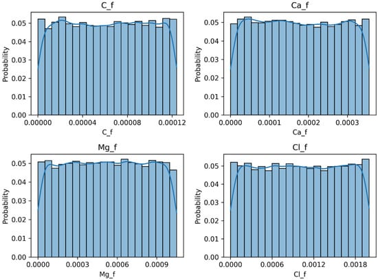
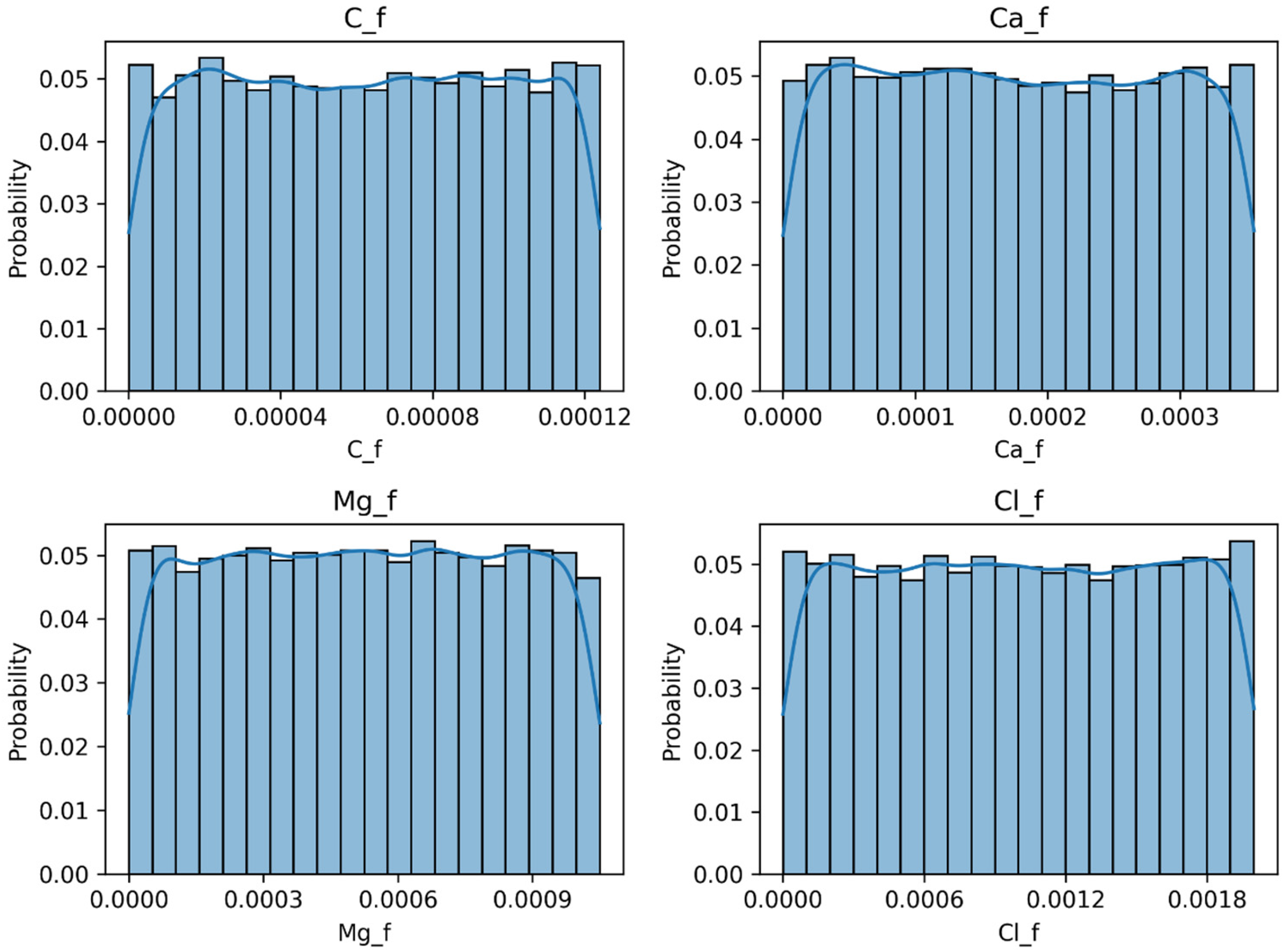
Figure 2 shows the histograms of the four input variables (features)—C_f, Ca_f, Mg_f, and Cl_f—used for surrogate model training. All features exhibit nearly uniform probability density distributions across their predefined ranges, confirming that the sampling strategy successfully generated a homogeneous coverage of the geochemical input space. Minor fluctuations in bin heights are attributed to finite sample size rather than systematic bias.

Figure 2. Histograms of uniformly sampled input features (C_f, Ca_f, Mg_f, Cl_f) used for surrogate model training, with overlaid kernel density estimation (KDE) curves indicating the empirical probability density distribution.

The uniform distributions ensure balanced representation of low- and high-concentration regimes, which is essential for capturing the nonlinear equilibrium behaviour associated with calcite dissolution under varying MgCl₂ conditions. Importantly, the absence of skewness or clustering indicates that any correlations learned by the neural network originate from the chemical equilibrium response computed with IPhreeqc, rather than from artefacts of the sampling procedure.

3.2. Phreeqc Results with Sampled Inputs

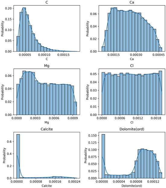
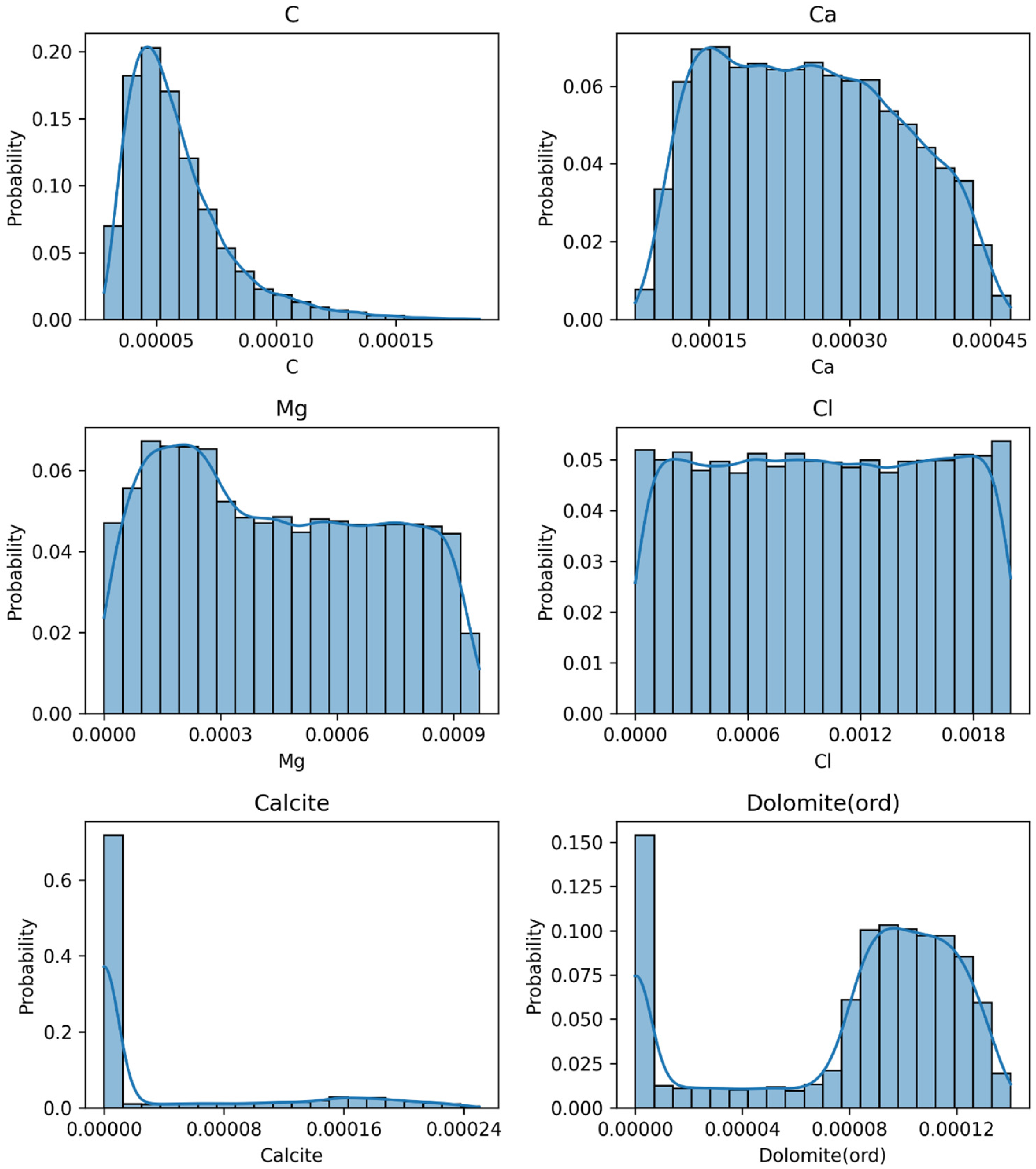
Figure 3 presents the histograms of the output variables (labels) obtained from the equilibrium calculations: aqueous species concentrations (C, Ca, Mg, Cl) and mineral amounts (Calcite and Dolomite (ord)). In contrast to the uniformly sampled inputs, the outputs exhibit strongly non-uniform and nonlinear distributions, reflecting the intrinsic thermodynamic constraints of the reactive system. Dissolved carbon (C) shows a positively skewed distribution with a pronounced peak at low concentrations and a long right tail, indicating that most equilibrium states correspond to low dissolved carbon, while higher concentrations occur less frequently. Calcium (Ca) and magnesium (Mg) concentrations display broader, moderately skewed distributions shaped by mineral saturation conditions, whereas the chloride (Cl) concentration remains approximately uniform due to its conservative behaviour in the system (non-reactive species).

Figure 3. Histograms of output variables (C, Ca, Mg, Cl, Calcite, Dolomite (ord)) obtained from equilibrium calculations, with overlaid kernel density estimation (KDE) curves representing the empirical probability density distributions.

Mineral phases exhibit highly non-Gaussian behaviour. Calcite shows a dominant peak near zero, indicating that in a large fraction of the sampled conditions calcite is either absent or present in very small amounts, with precipitation occurring only within a limited region of the parameter space. Dolomite (ord) presents a bimodal-type distribution, with a significant probability mass near zero and a second concentration range corresponding to precipitation-dominated conditions. These strongly skewed and discontinuous distributions highlight the nonlinear and threshold-controlled nature of mineral equilibrium reactions, which increase the complexity of surrogate modelling compared to the input feature space.

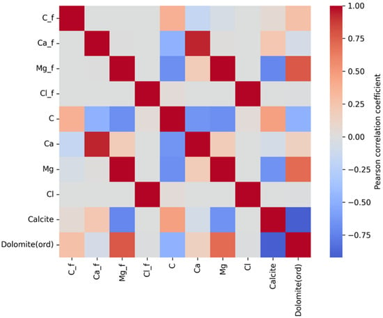
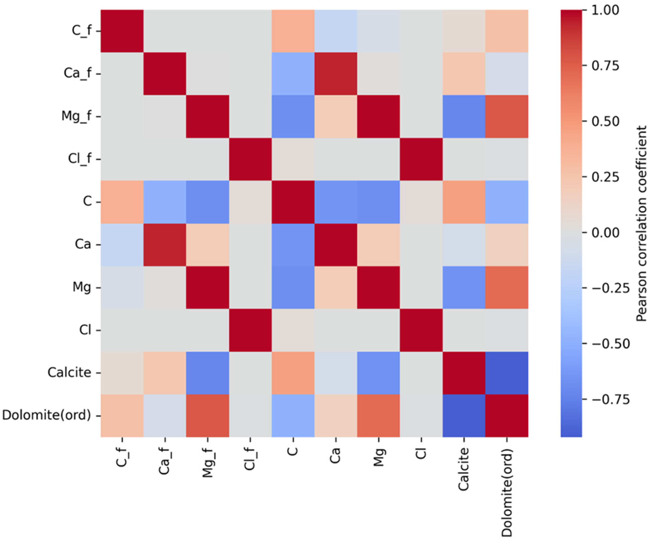
The correlation heatmap in Figure 4 illustrates the Pearson correlation coefficients between the input features (C_f, Ca_f, Mg_f, Cl_f) and the equilibrium outputs (C, Ca, Mg, Cl, Calcite, Dolomite (ord)). As expected from the uniform sampling strategy, the input features show negligible correlation among themselves, confirming statistical independence of the generated dataset. In contrast, strong correlations appear between certain inputs and their corresponding equilibrium concentrations, particularly Ca_f–Ca and Mg_f–Mg, indicating that initial bulk concentrations significantly influence their dissolved equilibrium states.

Figure 4. Pearson correlation coefficients values (heatmap type graph) of input features and equilibrium outputs, illustrating linear dependencies between initial chemical conditions and reactive equilibrium responses.

The mineral phases exhibit more complex relationships than separate chemical elements. Calcite shows s positive correlation with dissolved carbon (C) concentration and moderate dependence on Ca_f, reflecting its control by carbonate system equilibria. Dolomite (ord) is strongly positively correlated with Mg_f and Mg, and negatively correlated with Calcite, indicating competitive behaviour between Calcite and Dolomite. The pronounced negative correlation between Calcite and Dolomite (ord) highlights the thermodynamic coupling between these mineral phases, where conditions favouring Dolomite formation tend to suppress Calcite precipitation. Overall, Figure 3 confirms that nonlinear geochemical interactions, rather than simple linear dependencies, govern the reactive equilibrium system.

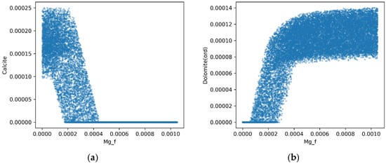
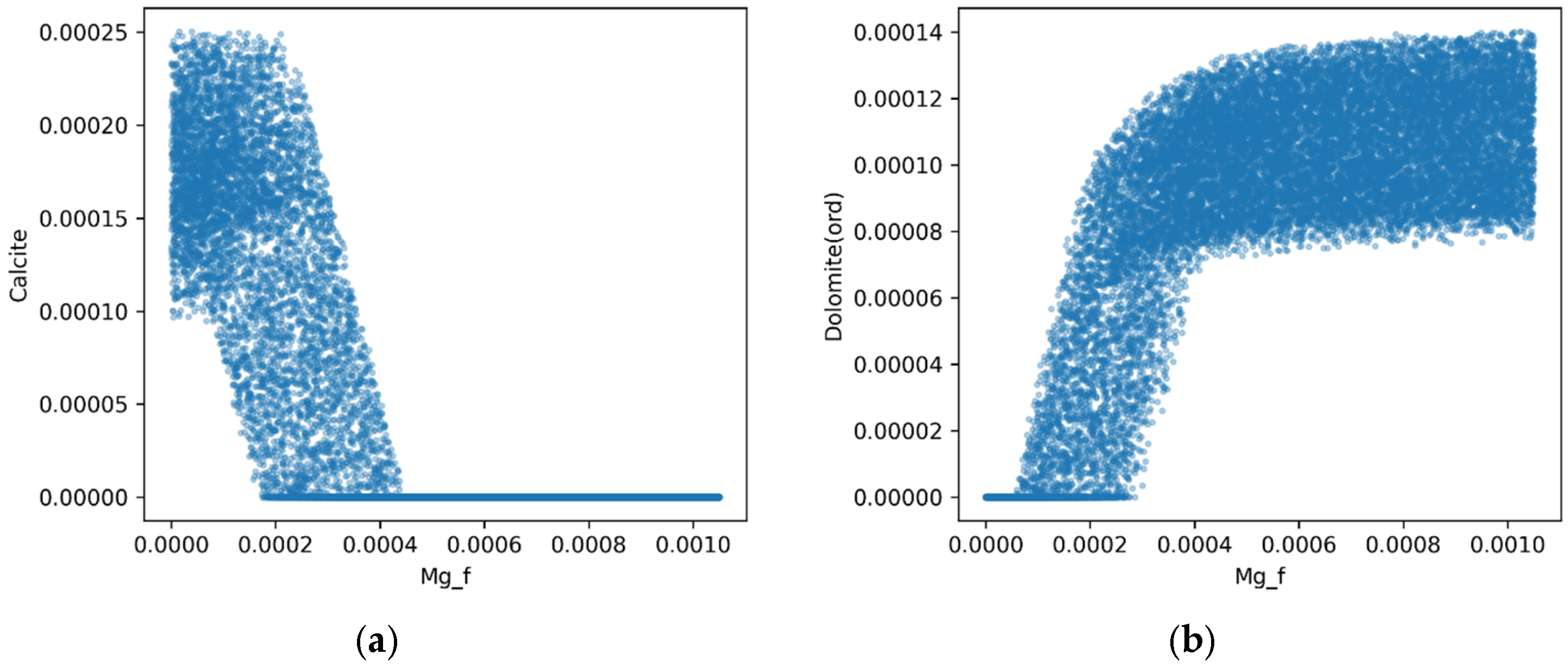
The scatter plots in Figure 5 highlight the most informative relationships among all variable pairs, specifically Mg_f–Calcite and Mg_f–Dolomite (ord). In the first plot (Figure 5a), a clear negative and strongly nonlinear relationship between Mg_f and Calcite is observed. At low Mg_f values, calcite precipitation spans a wide range and reaches its maximum values. As Mg_f increases, calcite rapidly decreases and eventually collapses to zero, forming a horizontal band at Calcite = 0. This pattern reflects the thermodynamic suppression under magnesium-rich conditions.

Figure 5. Scatter plots illustrating nonlinear mineral equilibrium responses to increasing magnesium concentration (Mg_f): (a) Calcite concentration versus Mg_f; (b) Dolomite (ord) concentration versus Mg_f.

In contrast, the Mg_f vs. Dolomite (ord) plot (Figure 5b) shows the opposite trend. Dolomite formation is negligible at very low Mg_f values but increases sharply beyond a threshold magnesium concentration and then approaches a saturation-like plateau. The curved shape indicates a nonlinear phase transition from calcite-dominated to dolomite-dominated conditions. These results complement the correlation heatmap by revealing the underlying nonlinear structure that cannot be fully captured by linear Pearson correlation coefficients alone.

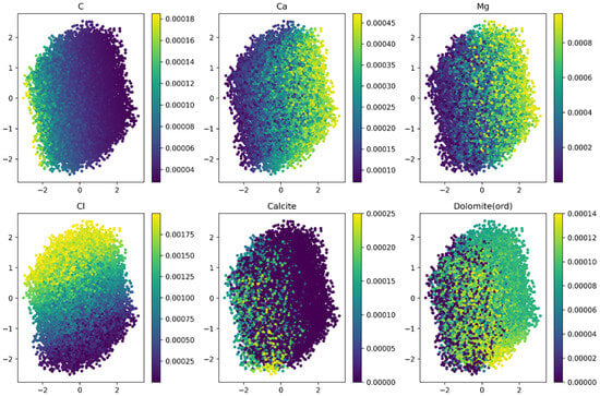
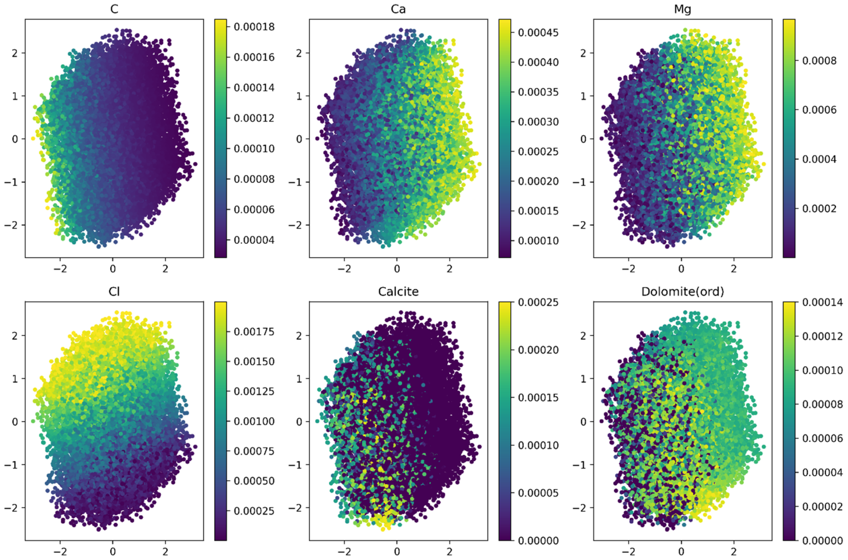
Figure 6 shows a two-dimensional projection of the dataset obtained using Principal Component Analysis (PCA), a statistical method that transforms the data into new axes representing directions of maximum variability. The first principal component (PC1), shown on the horizontal (x) axis, captures the largest variation in the dataset, while the second principal component (PC2), shown on the vertical (y) axis, captures the next largest variation and is orthogonal to PC1. These axes represent combinations of the original variables rather than individual physical quantities. Each subplot is coloured according to the magnitude of a different variable (C, Ca, Mg, Cl, Calcite, Dolomite (ord)). The projection reveals a continuous, structured distribution rather than distinct clusters, indicating that the geochemical states evolve smoothly across the sampled parameter space. The colour gradients for aqueous species, particularly Ca and Mg, are predominantly aligned along the PC1 direction, indicating that the dominant variability in the system is largely controlled by changes in calcium and magnesium concentrations.

Figure 6. Two-dimensional projection of the dataset using Principal Component Analysis (PCA). The axes (PC1—horizontal or x axis and PC2—vertical or y axis) represent directions of maximum variance in the data and correspond to combinations of the original variables. The dataset is coloured by aqueous species concentrations and mineral amounts to illustrate the global structure of reactive equilibrium states.

Additional insight is gained when examining the mineral phases. Calcite displays high values concentrated in a specific region of the projected space, with large areas showing near-zero amounts. In contrast, Dolomite (ord) shows an opposite spatial pattern, increasing in regions where Calcite diminishes. This complementary distribution further confirms the competitive mineral equilibria and phase transition behaviour previously observed in the scatter plots. Compared to the correlation heatmap and pairwise plots, this projection highlights the global structure of the dataset, demonstrating that the reactive system occupies a coherent nonlinear distribution governed by coupled carbonate equilibrium reactions rather than independent linear trends.

3.3. DNN Model Construction, Selection of Architecture

Based on the observed data structure in the histograms, scatter plots, and PCA projection, different hyperparameter configurations were systematically selected to evaluate their influence on surrogate model accuracy and training efficiency. The histograms revealed strongly skewed and threshold-controlled output distributions (especially for Calcite and Dolomite (ord)), while the scatter plots demonstrated pronounced nonlinear and phase-transition-like relationships. The PCA projection further indicated that the dataset forms a continuous but nonlinear distribution rather than separable clusters. Consequently, networks with varying depths, widths, activation functions, and learning rates were tested to assess their ability to capture smooth trends as well as sharp transitions in mineral formation. This structured comparison allowed for an evaluation of how architectural complexity and optimisation settings affect both the predictive fidelity and computational performance of the surrogate models.

3.4. Network Size

In Figure 7a, the network with a total of 22 neurons (i.e., computational units that determine the model’s capacity to represent nonlinear relationships) exhibits a smooth and monotonic decrease in both training and validation mean square error (MSE) over the 20 epochs. The training error drops rapidly during the first few epochs, indicating efficient learning of the dominant nonlinear relationships in the reactive equilibrium mapping, and then gradually converges toward a lower value. The validation curve closely follows the training curve throughout the training process, with no visible divergence, suggesting stable generalisation and absence of overfitting. However, the final MSE values remain slightly higher compared to the larger network (Figure 7b), indicating that the representational capacity of 22 neurons is sufficient but somewhat limited for fully capturing the complexity of the chemical response surface.

Figure 7. Comparison of Training and Validation MSE for Networks with 22 (a) and 50 (b) Neurons.

In Figure 7b, the network with 50 neurons demonstrates a similar convergence pattern but achieves consistently lower training and validation errors across all epochs. The model converges to a smaller final MSE, reflecting improved approximation capability due to increased network capacity. As in the 22-neuron case, the training and validation curves remain nearly overlapping, confirming stable optimisation and good generalisation. Additional experiments with 100 neurons produced virtually identical convergence behaviour and final error levels as the 50-neuron model, indicating that performance saturates around 50 neurons, and further increases in neuron quantity just increase computational cost without measurable gains in predictive accuracy.

In Figure 8a, the network with 50 neurons organised in a single hidden layer shows a steady decrease in both training and validation MSE over the training epochs. The training error drops sharply during the first epoch, followed by a more gradual and smooth convergence toward the final value. The validation curve closely follows the training curve throughout the optimisation process, indicating stable generalisation and absence of overfitting. However, the convergence is relatively moderate in speed and the final MSE remains slightly higher compared to the deeper architecture, suggesting that while a single hidden layer with sufficient width can approximate the nonlinear reactive mapping, its representational efficiency is somewhat limited.

Figure 8. Comparison of Training and Validation MSE for 1 (a) and 3 (b) Hidden-Layer Networks (50 Neurons Total).

In Figure 8b, the 50-neuron network distributed across three hidden layers (4–10–20–10–6 architecture) demonstrates faster convergence and consistently lower training and validation errors across all epochs. The deeper structure enables a more efficient hierarchical representation of the nonlinear geochemical equilibrium relationships, resulting in improved approximation accuracy. As in the single-layer case, the training and validation curves remain closely aligned, confirming robust generalisation. Additional experiments with four hidden layers yielded nearly identical convergence behaviour and final MSE values compared to the three-layer configuration, indicating that performance saturates at three hidden layers and that further increases in depth do not provide measurable improvements for the considered reactive system.

3.5. Activation Functions

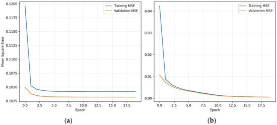
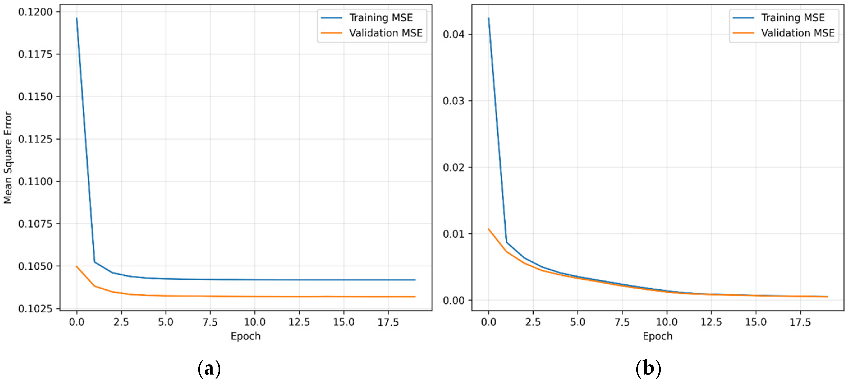
The comparison between ReLU (Figure 9a) and Tanh (Figure 9b) activation functions highlights notable differences in convergence behaviour under identical architectural and training settings. In the ReLU case, the training and validation losses decrease sharply during the first epoch but quickly reach a plateau, remaining nearly constant thereafter. This behaviour indicates premature stagnation of the optimisation process. While ReLU sometimes provided faster convergence in certain runs, repeated experiments revealed sensitivity to initialisation and training dynamics, occasionally leading to unstable learning or early saturation of the loss. In contrast, the Tanh activation exhibits a smoother and more gradual reduction in both training and validation MSE, with continuous improvement across epochs. The close alignment of training and validation curves and the absence of early plateauing suggest more consistent and stable convergence behaviour. Overall, Tanh demonstrated greater robustness across runs, whereas ReLU showed higher variability despite its potential for rapid initial learning.

Figure 9. Comparison of Training and Validation MSE for ReLu (a) and Tanh (b) Activation functions.

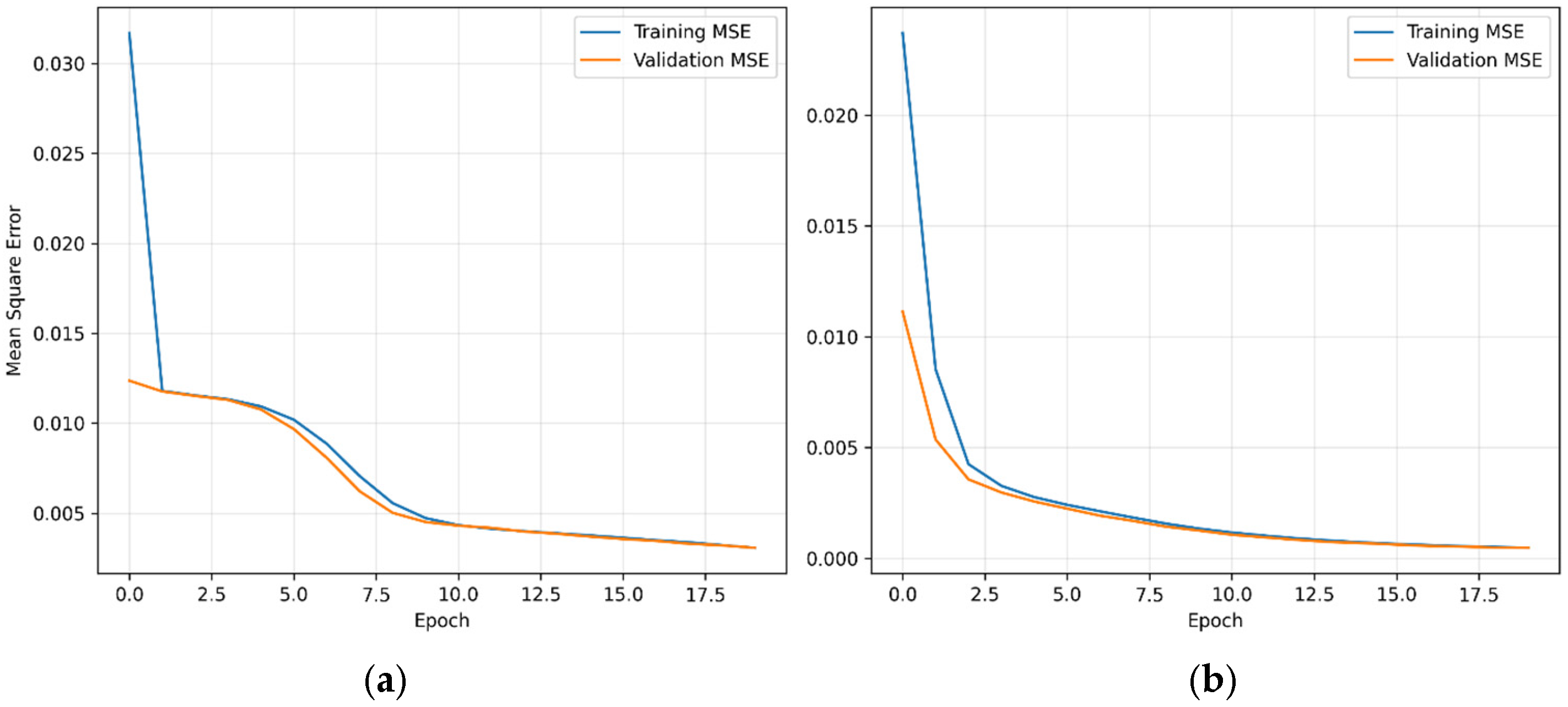
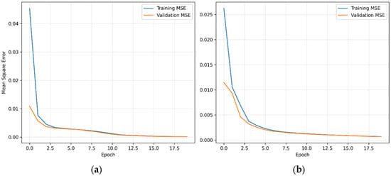
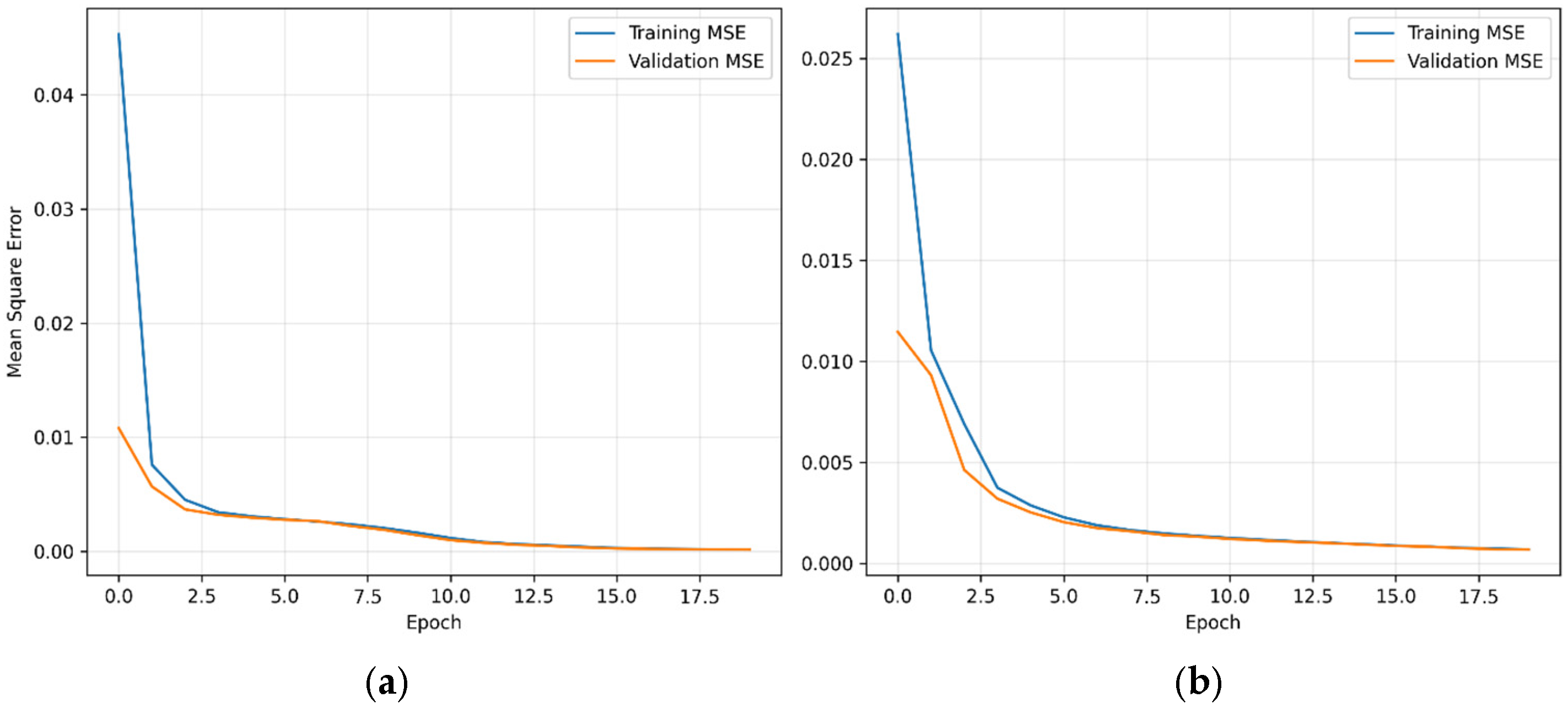
In Figure 10 the comparison between SiLU (a) and Tanh (b) activation functions indicates that Tanh achieves a more pronounced error reduction in this particular case. Although both activation functions exhibit stable and monotonic convergence with closely aligned training and validation curves, the Tanh model reaches substantially lower MSE values.

Figure 10. Comparison of Training and Validation MSE for SiLU (a) and Tanh (b) Activation functions.

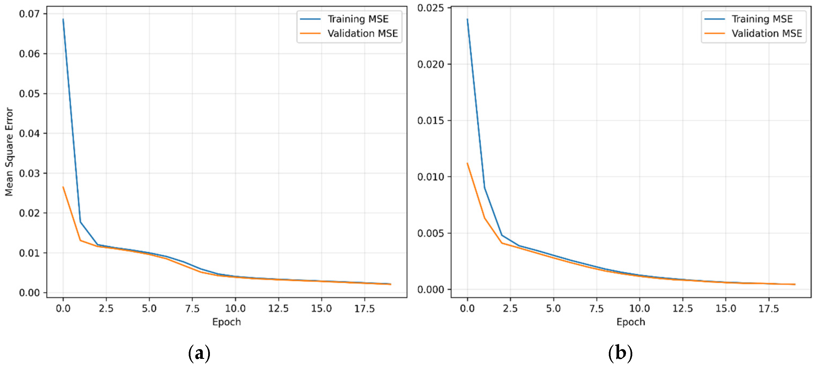
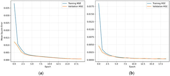
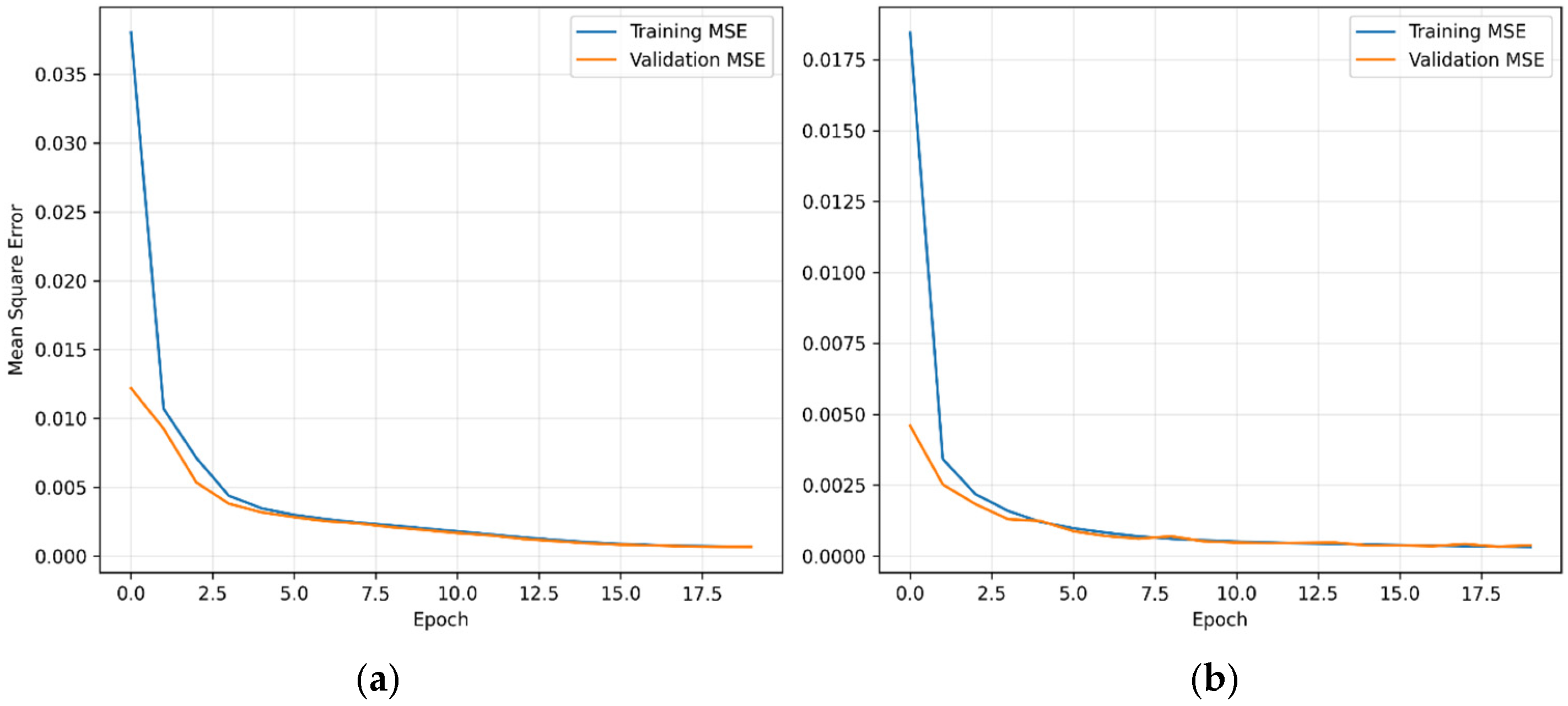
The comparison of batch sizes 32 (Figure 11a) and 8 (Figure 11b) shows that reducing the batch size leads to faster convergence and lower final MSE values. With batch size 32, both training and validation errors decrease smoothly but more gradually, reaching a moderate final error level. In contrast, batch size 8 exhibits a steeper initial decline and consistently achieves lower training and validation MSE across epochs. The smaller batch introduces greater stochasticity in the gradient updates, which can enhance exploration of the loss landscape and improve generalisation. For the considered reactive surrogate model, a batch size of 8 provides similar predictive accuracy compared to batch size 32, but smaller batches increase computational time per epoch due to more frequent weight updates.

Figure 11. Comparison of Training and Validation MSE for Batch Sizes 32 (a) and 8 (b).

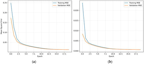
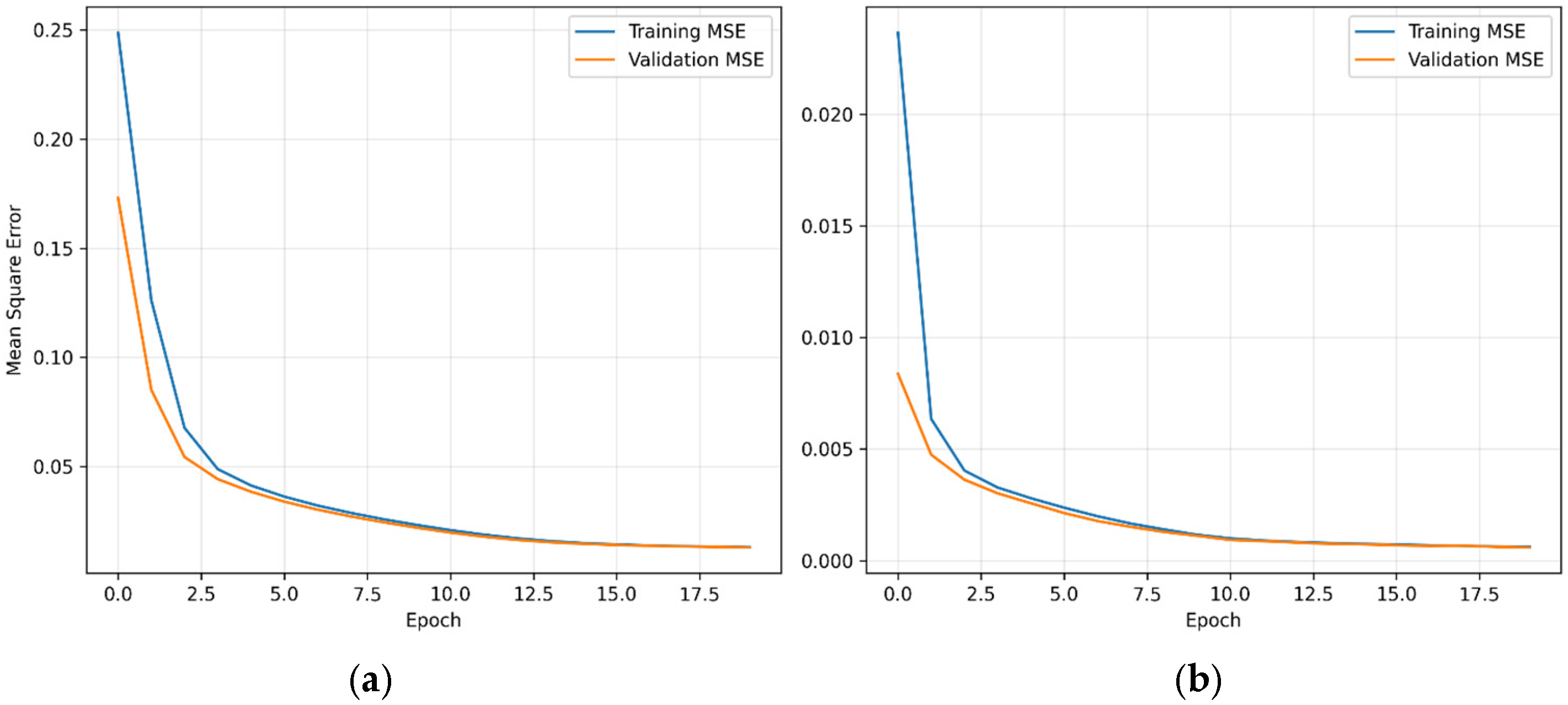
The comparison between batch sizes 1024 (Figure 12a) and 32 (Figure 12b) shows a clear advantage of the smaller batch size in terms of convergence speed and final accuracy. With batch size 1024, the training and validation MSE decrease smoothly but remain substantially higher throughout the training process, indicating slower optimisation and a limited ability to reach a low-error region within the same number of epochs. In contrast, batch size 32 exhibits a much steeper reduction in both training and validation errors, achieving significantly lower final MSE values. The smaller batch size introduces greater gradient variability, which helps the optimizer explore the loss landscape more effectively and escape shallow regions, leading to improved generalisation. Although large batches are computationally efficient per epoch, these results suggest that, for the considered reactive surrogate problem, moderate batch sizes such as 32 provide superior optimisation performance and predictive accuracy compared to very large batches like 1024.

Figure 12. Comparison of Training and Validation MSE for Batch Sizes 1024 (a) and 32 (b).

4. Conclusions

This study demonstrated that deep neural network (DNN) surrogate models can accurately reproduce the equilibrium geochemical calculations of Calcite dissolution and Dolomite precipitation generated with the IPhreeqc C++ API. By restricting the analysis strictly to the reactive chemical domain, without coupling to transport processes, the nonlinear mapping between initial aqueous composition (C_f, Ca_f, Mg_f, Cl_f) and post-equilibrium aqueous and mineral states was isolated and systematically evaluated. The results confirm that equilibrium speciation involving competitive carbonate reactions and magnesium-induced phase transitions can be reliably approximated by properly configured feed-forward neural networks.

The analysis of input–output relationships indicated that the reactive equilibrium dataset is characterised by smooth but nonlinear dependencies governed by thermodynamic constraints and mineral stability thresholds. Histograms, correlation analysis, scatter plots, and PCA projections showed that mineral phase transitions (Calcite dissolution and Dolomite precipitation) introduce sharp nonlinear features that must be captured by the surrogate model. Despite these complexities, the correctly parametrised surrogate models achieved high accuracy across the sampled chemical domain, with training and validation losses values closely aligned, indicating stable generalisation without overfitting.

The conducted parametric hyperparameter analysis revealed that surrogate model accuracy and training stability depend on network architecture and optimisation settings. Increasing neuron count improved accuracy up to a saturation threshold (approximately 50 neurons), beyond which no significant gains were observed. Distributing neurons across multiple hidden layers enhanced convergence efficiency, with three hidden layers providing an optimal balance between representational capacity and stability. Among the tested activation functions, Tanh showed more robust and consistent convergence behaviour compared to ReLU and SiLU for the considered equilibrium system. Batch size also significantly influenced optimisation dynamics, where moderate batch sizes (8–32) yielded faster convergence and lower final MSE compared to very large batches. These findings indicate that careful hyperparameter tuning is essential for chemically consistent surrogate modelling.

Overall, the results demonstrate that well-tuned DNN surrogate models provide an efficient and accurate alternative to repeated equilibrium calculations performed with chemical solver such as PHREEQC. Such surrogate models can be coupled with transport solvers to solve reactive transport problems in geochemical systems relevant to deep geological repository conditions and reduce computational cost while preserving accuracy within the predefined chemical domain.

References

- International Atomic Energy Agency (IAEA). Geological Disposal of Radioactive Waste; Technical Reports Series No. 413; International Atomic Energy Agency: Vienna, Austria, 2002. [Google Scholar]
- OECD Nuclear Energy Agency (NEA). The Handling of Timescales in Assessing Post-Closure Safety of Deep Geological Repositories; OECD/NEA: Paris, France, 2012. [Google Scholar]
- Steefel, C.I.; Appelo, C.A.J.; Arora, B.; Jacques, D.; Kalbacher, T.; Kolditz, O.; Lagneau, V.; Lichtner, P.C.; Mayer, K.U.; Meeussen, J.C.L.; et al. Reactive transport codes for subsurface environmental simulation. Comput. Geosci. 2015, 19, 445–478. [Google Scholar] [CrossRef] [Scilit]
- Narkunienė, A.; Grigaliūnienė, D.; Poškas, G. THC Modelling of Bentonite Barrier of Geological Repository in Granite and Its Impact on Long-Term Safety. Appl. Sci. 2024, 14, 7851. [Google Scholar] [CrossRef] [Scilit]
- Nardi, A.; Idiart, A.; Trinchero, P.; De Vries, L.M.; Molinero, J. Interface COMSOL–PHREEQC for reactive transport modelling of CO2 storage. Comput. Geosci. 2014, 69, 10–20. [Google Scholar] [CrossRef] [Scilit]
- Jacques, D.; Šimůnek, J.; Timmerman, A.; Van Genuchten, M.T. Modeling coupled hydrological and chemical processes: Long-term uranium transport simulation. Vadose Zone J. 2008, 7, 698–711. [Google Scholar] [CrossRef] [Scilit]
- Prommer, H.; Barry, D.A.; Zheng, C. MODFLOW/MT3DMS-based reactive multicomponent transport modeling. Ground Water 2005, 41, 247–257. [Google Scholar] [CrossRef] [Scilit] [PubMed]
- Parkhurst, D.L.; Appelo, C.A.J. Description of Input and Examples for PHREEQC Version 3–A Computer Program for Speciation, Batch-Reaction, One-Dimensional Transport, and Inverse Geochemical Calculations; U.S. Geological Survey Techniques and Methods, Book 6; USGS: Reston, VA, USA, 2013; Chapter A43.
- Prasianakis, N.I.; Laloy, E.; Jacques, D.; Meeussen, J.C.L.; Miron, G.D.; Kulik, D.A.; Idiart, A.; Demirer, E.; Coene, E.; Cochepin, B.; et al. Geochemistry and machine learning: Methods and benchmarking. Environ. Earth Sci. 2025, 84, 121. [Google Scholar] [CrossRef] [Scilit]
- Abadi, M.; Agarwal, A.; Barham, P.; Brevdo, E.; Chen, Z.; Citro, C.; Corrado, G.S.; Davis, A.; Dean, J.; Devin, M.; et al. TensorFlow: Large-Scale Machine Learning on Heterogeneous Distributed Systems. arXiv 2016, arXiv:1603.04467. [Google Scholar]
- Chollet, F. Keras. Available online: https://keras.io (accessed on 30 March 2026).
- Pedregosa, F.; Varoquaux, G.; Gramfort, A.; Michel, V.; Thirion, B.; Grisel, O.; Blondel, M.; Prettenhofer, P.; Weiss, R.; Dubourg, V.; et al. Scikit-learn: Machine Learning in Python. J. Mach. Learn. Res. 2011, 12, 2825–2830. [Google Scholar]
- McKinney, W. Data Structures for Statistical Computing in Python. In Proceedings of the 9th Python in Science Conference (SciPy 2010), Austin, Texas, 28 June–3 July 2010; pp. 51–56. [Google Scholar]
- Harris, C.R.; Millman, K.J.; van der Walt, S.J.; Gommers, R.; Virtanen, P.; Cournapeau, D.; Wieser, E.; Taylor, J.; Berg, S.; Smith, N.J.; et al. Array Programming with NumPy. Nature 2020, 585, 357–362. [Google Scholar] [CrossRef] [Scilit] [PubMed]
- Hunter, J.D. Matplotlib: A 2D Graphics Environment. Comput. Sci. Eng. 2007, 9, 90–95. [Google Scholar] [CrossRef] [Scilit]
- Waskom, M.L. Seaborn: Statistical Data Visualization. J. Open Source Softw. 2021, 6, 3021. [Google Scholar] [CrossRef] [Scilit]
- Hummel, W.; Berner, U.; Curti, E.; Pearson, F.J.; Thoenen, T. Nagra/PSI Chemical Thermodynamic Data Base 01/01; Universal Publishers: Parkland, FL, USA, 2002. [Google Scholar]
- Appelo, C.A.J.; Postma, D. Geochemistry, Groundwater and Pollution, 2nd ed.; CRC Press: Boca Raton, FL, USA, 2005. [Google Scholar]
- Kolditz, O.; Görke, U.-J.; Shao, H.; Wang, W. Thermo-Hydro-Mechanical-Chemical Processes in Porous Media: Benchmarks and Examples; Springer: Berlin, Germany, 2012. [Google Scholar]
Disclaimer/Publisher’s Note: The statements, opinions and data contained in all publications are solely those of the individual author(s) and contributor(s) and not of MDPI and/or the editor(s). MDPI and/or the editor(s) disclaim responsibility for any injury to people or property resulting from any ideas, methods, instructions or products referred to in the content. |
© 2026 by the authors. Licensee MDPI, Basel, Switzerland. This article is an open access article distributed under the terms and conditions of the Creative Commons Attribution (CC BY) license.