Inertia Estimation in High-RES Power Systems Using Small-Signal Power Injection

Abstract

This paper proposes a continuous inertia estimation framework for transmission-level power systems with high renewable energy penetration, using a battery energy storage system (BESS) as a controllable small-signal power injection source. The proposed framework integrates BESS-based active power injection, a two-stage signal-smoothing scheme, and a rate-of-change-of-frequency (RoCoF)-based estimation mechanism to enable continuous inertia estimation without relying on major disturbance events. With noise-robust processing and moving-window analysis, the framework can reliably track inertia variations under noisy measurement conditions and diverse operating scenarios. The framework is validated on the IEEE 39-bus system under renewable energy source (RES) penetration levels of 0%, 10%, 20%, and 30%. The estimation error remains within ±3.5% across all scenarios, ranging from 1.26% at 0% RES penetration to 3.43% at 30% penetration. In addition, the estimated inertia closely follows the theoretical decrease from 3.20 s to 2.22 s as RES penetration increases. These results demonstrate the accuracy and robustness of the proposed framework for continuous inertia monitoring in low-inertia power systems with high-RES penetration.

1. Introduction

With increasing penetration of renewable energy sources (RES), modern power systems are experiencing a progressive reduction in rotational inertia. Unlike conventional synchronous generators, most RES units are interfaced with the grid through power electronic converters and, without virtual inertia or grid-forming control, provide little or no inherent inertial support. As a result, the rate of change of frequency (RoCoF) following power imbalances can increase significantly, posing growing challenges to frequency stability and secure system operation [1,2]. Under such conditions, accurate estimation of system inertia has become increasingly important for the monitoring, operation, and control of high-RES power systems [3,4].

Most existing inertia estimation methods rely on large disturbance events, such as generator outages or major load changes, and estimate system inertia from the resulting frequency response using the swing equation [5,6,7,8,9]. These methods are commonly implemented using phasor measurement units (PMUs) or wide-area measurement systems (WAMS) and can provide useful inertia information following major events [10,11,12]. However, because they depend on infrequent disturbances, their applicability to continuous monitoring and real-time tracking of inertia variations is limited.

To improve timeliness, recent studies have explored inertia estimation methods based on ambient measurements of frequency and power under normal operating conditions. Several studies have shown that PMU-based ambient data can be used to estimate online inertia variations, including area-level and system-wide inertia in interconnected power systems [13,14,15,16,17,18,19]. These findings indicate that ambient measurements can provide useful information on inertia dynamics without requiring large disturbances.

In addition to passive approaches, recent studies have investigated active inertia estimation methods that use controllable excitation signals to improve estimation timeliness and identifiability. Existing work has demonstrated the feasibility of BESS-based inertia estimation in microgrids and small islanded systems, including real-time estimation methods using local frequency measurements and small-signal power injection [20,21,22]. These results suggest that active excitation can serve as a practical alternative to disturbance-based estimation without disrupting normal operation. However, most of these methods have been validated only in microgrids or small-scale islanded systems. Their applicability to transmission-level power systems with multi-area structures, high RES penetration, and non-uniform regional inertia distribution remains insufficiently investigated.

Motivated by this research gap, this paper proposes a BESS-based active inertia estimation framework for a multi-area transmission-level power system. The proposed framework employs controllable small-signal power injection to excite system frequency dynamics and combines this mechanism with a two-stage signal filtering process to improve robustness under noisy measurement conditions. The framework is evaluated under operating scenarios with different RES penetration levels and uneven regional inertia distribution to assess its feasibility and estimation performance. The results show that the proposed framework can maintain stable and accurate inertia estimation across a range of operating conditions, indicating its potential for continuous inertia monitoring in future low-inertia transmission systems.

The remainder of this paper is organized as follows: Section 2 introduces the theoretical background of inertia estimation. Section 3 presents the signal processing methods. Section 4 describes the test system and simulation scenarios. Section 5 evaluates the proposed method through simulations, and Section 6 concludes the paper.

2. Inertia Response and Estimation Method

This section introduces the frequency response, the fundamentals of inertia, and the inertia estimation method used in this paper.

2.1. Background of Frequency Response

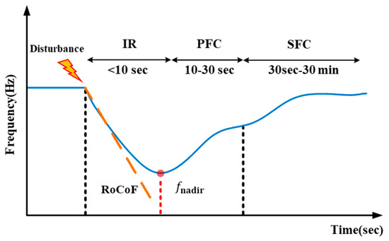
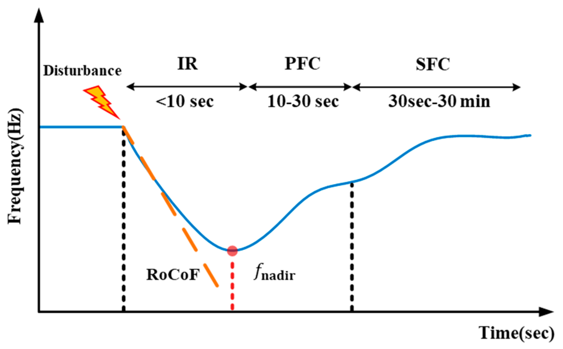
When a supply–demand imbalance occurs in a power system, the frequency response can be divided into three stages: inertial response (IR), primary frequency control (PFC), and secondary frequency control (SFC), as shown in Figure 1. When a sudden load increase or generator outage occurs, the rotational kinetic energy stored in synchronous generator rotors is released to the grid and forms the initial inertial response. This response provides instantaneous power support at the onset of the disturbance, thereby reducing the RoCoF and alleviating the frequency nadir. Subsequently, primary frequency control is provided by governor response, which gradually arrests and recovers the frequency, typically over a time scale of several to tens of seconds (e.g., 10–30 s). Finally, secondary frequency control, implemented via automatic generation control (AGC), restores the system frequency to its nominal value.

Figure 1. Frequency response of the power system after disturbance.

2.2. Theoretical Background

In conventional power systems, synchronous generators provide the dominant contribution to system inertia. The inertia constant of a synchronous generator determines the kinetic energy stored in the rotor and, consequently, influences the RoCoF and frequency regulation capability. This section introduces the definition of the inertia constant and its mathematical formulation [23].

The rotational inertia of a synchronous generator is determined by the rotor mass distribution and geometry. The corresponding kinetic energy stored in the rotating parts is given by:

$$E_{\mathit{gen}}={\displaystyle \frac{J{\omega }^2}{2}}$$

(1)

In (1), $E_{\mathit{gen}}$ represents the kinetic energy stored in the rotating parts of the synchronous machine; $J$ denotes the rotor-system moment of inertia, and $\omega$ is the mechanical angular speed.

From this relationship, it can be observed that the magnitude of the moment of inertia is purely determined by the physical dimensions and mass distribution of the rotor, and is not directly dependent on the electrical power output of the synchronous machine.

$$H_{\mathit{gen}}={\displaystyle \frac{E_{\mathit{nom}}}{S_{\mathit{gen}}}}={\displaystyle \frac{J{\omega }_N^2}{2S_{\mathit{gen}}}}$$

(2)

In (2), $E_{\mathit{nom}}$ represents the kinetic energy of the synchronous machine at its rated speed; $S_{\mathit{gen}}$ denotes the rated apparent power of the synchronous machine; and ${\omega }_N$ is the rated mechanical angular speed of the synchronous machine.

In conventional power systems, where system inertia mainly originates from synchronous generators, the equivalent inertia constant can be represented as the weighted average of the inertia constants of all synchronous generators, as shown below:

$$H_{\mathit{sys}}=\sum _{i=1}^N{\displaystyle \frac{H_{\mathit{gen},i}{S}_{\mathit{gen},i}}{S_{\mathit{sys}}}}$$

(3)

In (3), $H_{\mathrm{sys}}$ and $H_{\mathit{gen},i}$ represent the system equivalent inertia constant, the inertia constant of the i-th synchronous generator. Similarly, $S_{\mathit{sys}}$ and $S_{\mathit{gen},i}$ denote the total system capacity and the rated capacity of the generator.

With the increasing integration of RESs such as wind and solar power, the sources of inertia in the power grid are no longer limited to the rotational kinetic energy of synchronous machine rotors. To reflect this change, the equivalent inertia constant can be further extended as follows:

$$H_{\mathit{sys}}={\displaystyle \frac{{\sum }_{i=1}^{N_G}{H}_{\mathit{gen},i}{S}_{\mathit{gen},i} +\sum _{k=1}^{N_{\mathit{RES}}}{H}_{res,k}{S}_{res,k}}{S_{\mathit{sys}}}}$$

(4)

In (4), $N_G$ represents the number of synchronous generators participating in the calculation, and $N_{RES}$ denotes the number of RES units. $H_{\mathrm{res},k}$ is the equivalent virtual inertia constant of the k-th RES unit, and $S_{\mathrm{res},k}$ represents its rated capacity.

As the rotational inertia provided by synchronous generators gradually decreases, the influence of equivalent inertia from the load side and RES units on the system becomes increasingly significant. In particular, frequency-dependent loads and RESs or energy storage systems connected through power electronic converters can, through appropriate control strategies, participate in voltage and frequency regulation, thereby significantly altering the overall inertia characteristics.

This transformation reduces the inherent inertial support capability of the system, thereby requiring additional spinning reserve to maintain frequency stability. Consequently, the effective system inertia becomes a critical indicator, and its quantification and analysis form an essential foundation of this paper.

2.3. Proposed Inertia Estimation Framework

The swing equation describes the electromechanical dynamics of a synchronous machine, specifically the rotor acceleration or deceleration that occurs following a system disturbance. When formulated in terms of system frequency, the swing equation can be expressed as shown in (5).

$${\displaystyle \frac{2H}{f_0}}{\displaystyle \frac{df}{dt}}=P_{m\left(\mathit{pu}\right)}-P_{e\left(\mathit{pu}\right)}$$

(5)

In (5), $P_{m\left(\mathit{pu}\right)}$ denotes the mechanical power supplied by the prime mover, whereas $P_{e\left(\mathrm{pu}\right)}$ represents the electrical power output of the synchronous generator. The nominal system frequency is denoted by $f_0$, and ${\displaystyle \frac{df}{dt}}$ denotes the RoCoF. These variables collectively characterize the electromechanical power balance that governs the system’s dynamic behavior following a disturbance.

Based on the swing equation, when $P_{m\left(\mathit{pu}\right)}$ and $P_{e\left(\mathit{pu}\right)}$ are approximately balanced, the power injected into the grid by the BESS, $P_{\mathit{BESS}}$, can be incorporated into the formulation. Under this condition, the relationship can be expressed as shown in (6).

$${\displaystyle \frac{2H}{f_0}}{\displaystyle \frac{df}{dt}}=P_{m\left(\mathit{pu}\right)}-P_{e\left(\mathit{pu}\right)}+P_{\mathit{BESS}}=\Delta P$$

(6)

In this context, when the short-term variations in mechanical and electrical power within the system are negligible, the condition $P_{m\left(\mathit{pu}\right)}\approx$ $P_{e\left(\mathit{pu}\right)}$ can be reasonably assumed. Under this assumption, the swing equation can be further simplified, and the corresponding expression for estimating the equivalent system inertia constant $H$ can be derived. The resulting formulation is presented in (7).

$$H={\displaystyle \frac{\Delta P\hspace{0.17em}{f}_0}{2RoCoF}}$$

(7)

Finally, by applying a known and controllable power perturbation $\Delta P$ and combining it with the real-time measurements of the RoCoF, the equivalent system inertia can be estimated.

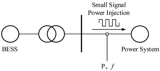
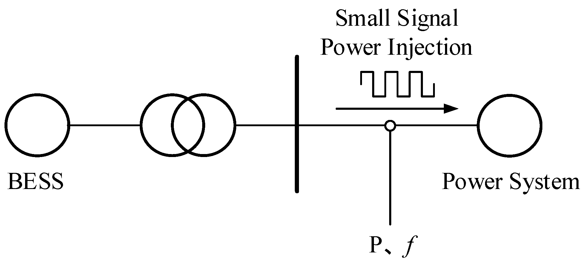
As shown in Figure 2, the BESS injects a controllable small-signal power into the power system, while the terminal frequency $f$ and active power $P_{\mathit{BESS}}$ are measured.

Figure 2. Small-signal power injection from the BESS into the power system.

The estimated inertia $H_{est}$ is compared with the system inertia $H_{sys}$ to quantify the estimation error. The percentage error, denoted as $PE\%$, is defined in (8). This metric is used to evaluate the accuracy of $H_{est}$ under each scenario and is adopted in the subsequent sections.

$$PE\%={\displaystyle \frac{|H_{sys}-H_{est}|}{H_{sys}}}\times 100\%$$

(8)

3. Signal Processing Method

This paper considers practical operating conditions in real power systems by incorporating measurement noise and appropriate data-processing procedures so that the analyzed signals better reflect real-world behavior. The complete signal-processing and estimation workflow is shown in Figure 3, which summarizes the key steps that connect noisy measurements to the final inertia estimation result. It includes reading the measured frequency $f$ and power P, superimposing measurement noise, and conditioning the signals through digital filtering. A two-stage filtering scheme is adopted to improve signal quality while preserving the frequency dynamic characteristics required for inertia estimation. First, a Savitzky–Golay filter is applied to smooth the signals, reducing high-frequency measurement noise while preserving the main signal trend and features. Then, discrete wavelet transform (DWT) is used for multi-resolution denoising to further remove residual noise components. The resulting processed frequency signal is then used to compute the inertia constant H based on the swing equation.

Figure 3. Data processing and computational flow.

3.1. Noise Addition Method

This paper uses the PSS^®E simulation platform to build a power system model and simulate the power injection behavior of the BESS, allowing the resulting frequency response to be observed for inertia estimation. However, PSS^®E does not include measurement noise or signal disturbances that commonly appear in real systems. To improve the accuracy and practicality of the proposed real-time inertia estimation method, this paper adds appropriate stochastic noise to the simulated data to reflect field measurements. Since these disturbances are random in nature, and Gaussian white noise is commonly encountered in measurement processes [24,25], this paper adopts Gaussian white noise as the noise source.

3.2. Savitzky–Golay Filtering

In the first stage of filtering, this paper employs a Savitzky–Golay filter, which is a numerical smoothing technique based on local polynomial regression. The objective of this filter is to attenuate high-frequency noise while preserving essential signal characteristics, including peaks, slopes, and local curvature, thereby preventing the loss of important dynamic features. The Savitzky–Golay method operates by selecting a symmetric sliding window of odd length centered on each time sample and fitting a polynomial of a specified order to the data points within the window. The value of this polynomial evaluated at the center of the window is then taken as the smoothed output. This procedure is applied sequentially across the entire dataset to achieve effective noise reduction without excessively distorting the underlying signal behavior [26,27].

Assume an s-order polynomial $f_i$. After applying the smoothing operation to the frequency samples, the resulting linear combination $\widehat{f_i}$ can be expressed as follows:

$$f_i=\sum _{j=0}^s{a_s}_j\cdot i^j=a_{s_0}+a_{s_1}\cdot i+a_{s_2}\cdot i^2+\cdots +a_{s_s}\cdot i^s$$

(9)

$$\widehat{f_i}=\sum _{k=-L}^L{c}_k\cdot \widetilde{f_{i+k}}=c_{-L}\cdot \widetilde{f_{i-L}}+c_{-L+1}\cdot \widetilde{f_{i-L+1}}+\cdots +c_L\cdot \widetilde{f_{i+L}}$$

(10)

Here, i denotes the position of the observation point, ${a_s}_j$ represents the polynomial coefficients, $\widehat{f_i}$ is the smoothed frequency value, $\widetilde{f_{i+k}}$ is the original noise-contaminated frequency sample, and $c_k$ denotes the smoothing weights. The objective is to determine the optimal set of $c_k$ such that:

$$E=\sum _{k=-L}^L{\left(f_i^k-\widetilde{f_{i+k}}\right)}^2=\sum _{k=-L}^L{\left[\left(\sum _{j=0}^s{a_s}_j\cdot i^j\right)-\widetilde{f_{i+k}}\right]}^2$$

(11)

Here, $E$ denotes the sum of squared errors over all samples within the moving window. The polynomial coefficients are determined by minimizing $E$, thereby obtaining the best local polynomial fit for the noisy frequency signal. Taking the partial derivative of $E$ with respect to each polynomial coefficient and setting it to zero yields:

$${\displaystyle \frac{\partial E}{\partial {a_s}_j}}=2\sum _{k=-L}^L\left[\left(\sum _{j=0}^s{a_s}_j\cdot i^j\right)-\widetilde{f_{i+k}}\right]i^r=0$$

(12)

Rearranging (12) gives:

$$\sum _{k=-L}^L\widetilde{f_{i+k}}·i^r=\sum _{j=0}^s{a_s}_j\sum _{k=-L}^L{i}^{j+r}$$

(13)

Here, (12) and (13) are used only in the Savitzky–Golay filtering stage to determine the local polynomial coefficients for smoothing the noisy frequency signal within each moving window. Their purpose is to preserve the local dynamic characteristics of the frequency signal before the subsequent DWT-based denoising and RoCoF calculation. In (13), $r = 0, 1, 2, \dots , s$ and $i = -L, -L+1, \dots , L$, where $L$ denotes the half-width of the moving window, and (13) can then be written in matrix form for computational implementation. Accordingly, the matrix $A_{i,r}$ is defined as follows:

$$A_{i,r}=\left[\begin{array}{cccc}{\left(-L\right)}^0& {\left(-L\right)}^1& \cdots & {\left(-L\right)}^s\\ {\left(-L+1\right)}^0& {\left(-L+1\right)}^1& \cdots & {\left(-L+1\right)}^s\\ ⋮& ⋮& \ddots & ⋮\\ 0^0& 0^1& \cdots & 0^s\\ ⋮& ⋮& \ddots & ⋮\\ L^0& L^1& \cdots & L^s\end{array}\right]$$

(14)

The corresponding expressions in matrix form are given in (15a)–(15c).

In (15a), the normal equation obtained from the least-squares fitting is shown, and (15b) provides its closed-form solution.

In the Savitzky–Golay formulation, the smoothing weights $c_k$ correspond to the coefficients that yield the polynomial value at the center of the window, giving:

$$\left(A^{T}A\right)\cdot a=A^T\tilde{f}$$

(15a)

$$a={\left(A^{T}A\right)}^{-1}{A}^T\tilde{f}$$

(15b)

$${\left[{\left(A^{T}A\right)}^{-1}{A}^T\right]}_{1\times \left(2L+1\right)}$$

(15c)

Finally, the smoothed frequency signal can be obtained by applying the weight vector $c_k$ to the noisy frequency measurements, as expressed in

$$f_{\mathrm{smooth}}=c_k\cdot f_{\mathrm{noisy}}$$

(16)

In (16), $f_{\mathrm{smooth}}$ denotes the smoothed frequency value, while $f_{\mathrm{noisy}}$ represents the original frequency samples containing disturbances and measurement noise. To compute each smoothed frequency point, the sample at the target time and its $L$ neighboring points on both sides—i.e., a total of $2L+1$ frequency samples—are used as the input for the polynomial fitting. This sliding-window procedure effectively suppresses high-frequency noise and mitigates its impact on the frequency signal, thereby improving the stability and reliability of the subsequent frequency estimation.

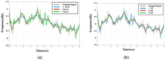
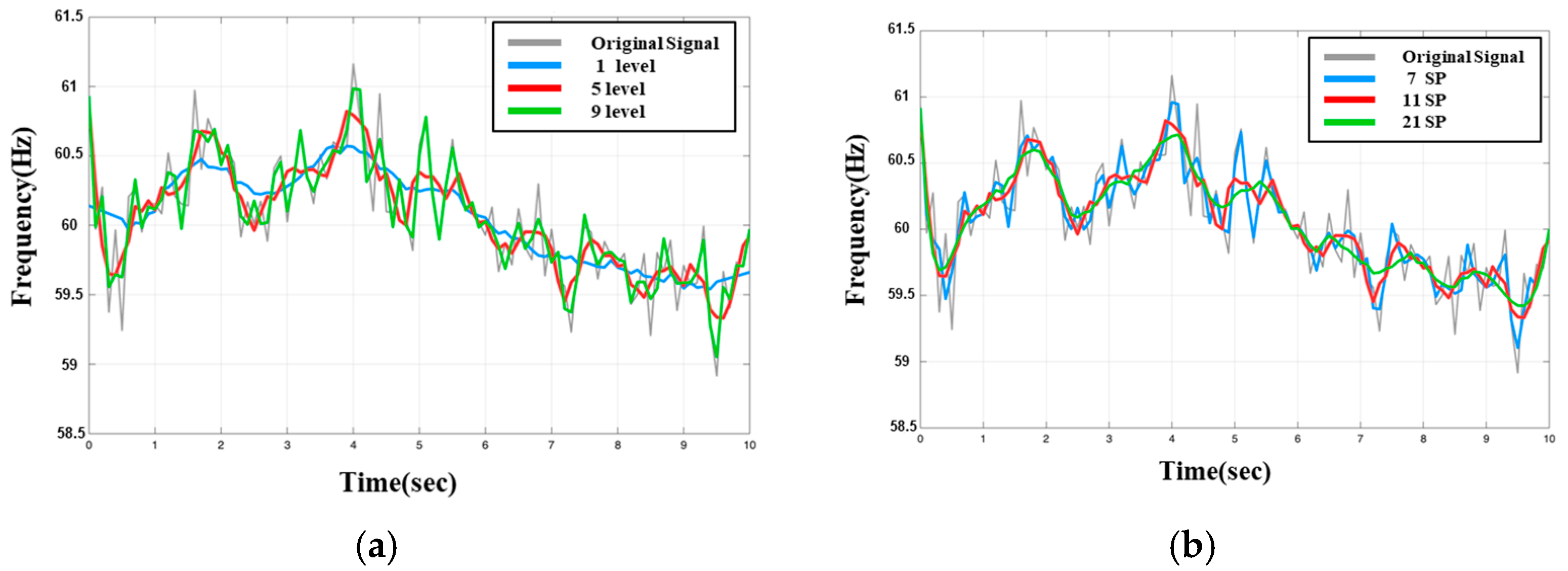
The filter parameters were adjusted based on the characteristics of the target signal and the analysis requirements to balance smoothing and feature preservation. As shown in Figure 4a,b, the filter reduced high-frequency measurement noise while preserving the main dynamic changes in the frequency signal.

Figure 4. Savitzky–Golay filtering results: (a) different polynomial orders; (b) different window lengths.

As shown in Figure 4a, with the window length fixed at 11, a lower polynomial order provides stronger smoothing but may suppress important signal details, whereas a higher polynomial order preserves more local features but is more sensitive to noise. As shown in Figure 4b, with the polynomial order fixed at 5, a shorter window length retains more local variations but offers weaker noise suppression, while a longer window length may lead to over-smoothing. Based on the test results, a polynomial order of 5 and a window length of 11 were selected for subsequent analysis.

3.3. DWT-Based Frequency Extraction

To further improve frequency-signal quality and suppress noise-induced fluctuations, this paper adopts the wavelet transform in the second-stage signal processing. Wavelet transforms are generally categorized as the continuous wavelet transform (CWT) and the DWT. The DWT decomposes a signal into multiple frequency bands in a multiresolution (hierarchical) manner. Because the frequency data used in this paper are discrete-time sequences, the DWT is selected for the second-stage processing. The DWT formulation is given in (17).

$$DWT\left(s,m,k\right)={\displaystyle \frac{1}{\sqrt{a}}}\sum _{n}S\left(n\right){\Psi }^{*}\left({\displaystyle \frac{k-b}{a}}\right)$$

(17)

where $S\left(n\right)$ denotes the value of the discrete signal at the n sampling point (i.e., the sample sequence). The index m represents the scale level, which determines the degree of dilation of the wavelet; the corresponding scale parameter is typically discretized as a = $a_0^m$. The index k is the translation (or position) index, specifying the time location associated with each wavelet coefficient. Ψ (⋅) is the mother wavelet function. The parameter b is the translation parameter used to shift the wavelet to a specified position, which is commonly discretized as ${b=nb}_{0}a$. The normalization factor $1/\sqrt{a}$ is introduced to preserve wavelet energy across different scales, ensuring the comparability of coefficients at different scale levels.

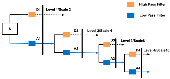
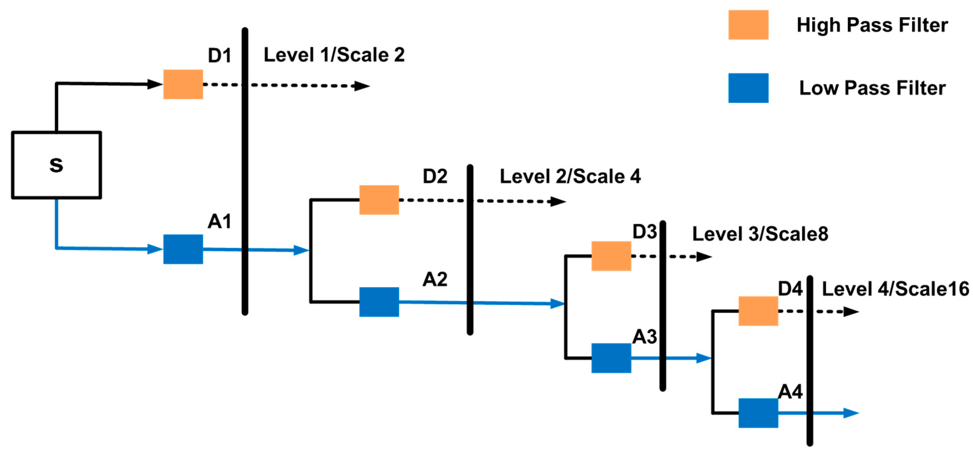
The DWT performs multilevel decomposition of the original signal by successively passing it through high-pass and low-pass filters. As shown in Figure 5, the decomposition process of the DWT is presented [28]. The original signal is first passed through a pair of high-pass and low-pass filters and decomposed into the detail component D1 and the approximation component A1. Subsequently, the same operation is applied only to the approximation component A1, yielding D2 and A2, and this procedure is recursively repeated until the predefined decomposition level is reached. At each level, the detail components (e.g., D1 to D4) progressively extract high-frequency information from different frequency bands, while the approximation components (e.g., A1 to A4) increasingly represent the low-frequency content of the signal. After each down sampling operation, the signal length is reduced to half of that at the previous level, resulting in a multiresolution analysis in which time resolution decreases and frequency resolution increases with the decomposition level.

Figure 5. Multilevel decomposition using DWT.

This paper adopts sym4 as the mother wavelet for denoising [29,30]. Based on preliminary testing, the signal is decomposed to the seventh level, yielding A7 and D1–D7. This decomposition improves noise suppression while preserving the signal characteristics required for subsequent RoCoF calculation and inertia estimation.

3.4. Moving-Window RoCoF Calculation

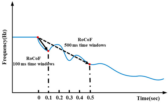
In power system operation and monitoring, the RoCoF, defined as the time derivative of frequency, is a key indicator. RoCoF reflects the speed of frequency variation following a disturbance and is widely used to assess the severity of power imbalance, support the estimation of equivalent system inertia, and serve as a triggering criterion for protection relays. Common approaches for RoCoF calculation include numerical differentiation of frequency signals and linear fitting using a moving measurement window. These methods are highly dependent on the selection of the measurement window.

As shown in Figure 6, different window lengths result in noticeable differences in the calculated RoCoF. When the window is too short, measurement noise or short-term frequency fluctuations may be included in the calculation, thereby degrading estimation accuracy. Conversely, an excessively long window may smooth out rapid frequency variations, leading to an underestimation of RoCoF. Therefore, the measurement window length is a critical factor in RoCoF calculation. Window lengths in the range of 20 to 500 ms are commonly adopted [31,32,33], depending on the application and operating conditions. In this paper, a window length of 200 ms is adopted to capture the transient variations caused by small disturbances.

Figure 6. RoCoF calculation with different window sizes.

4. Test System Model

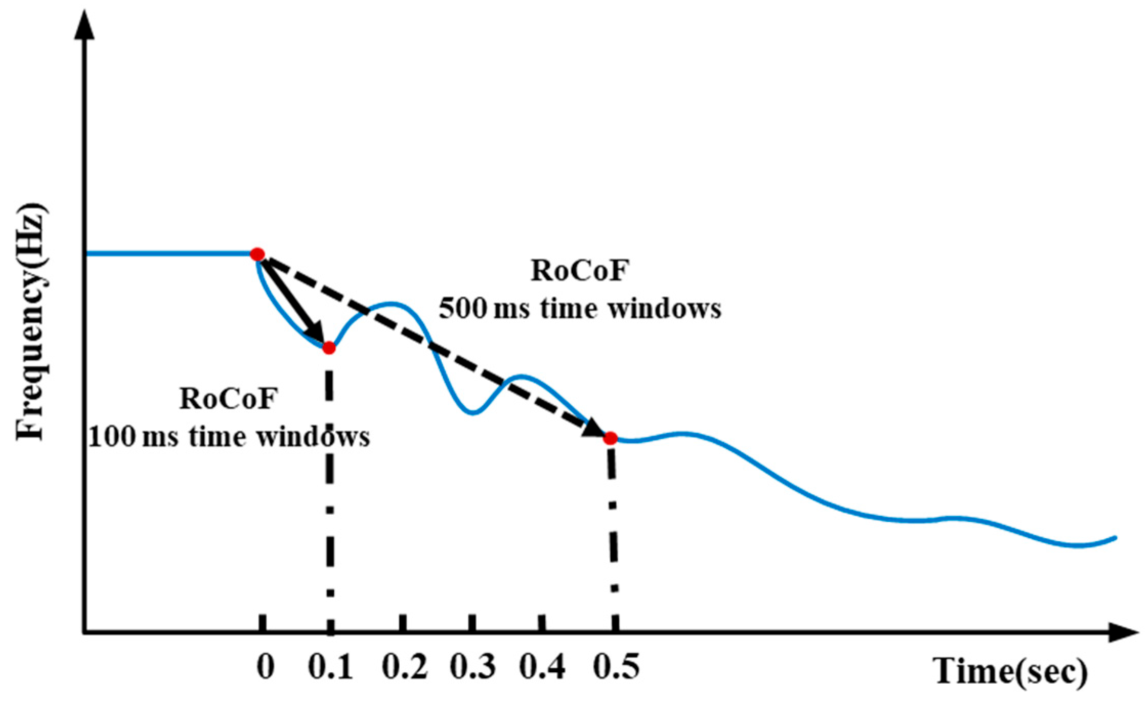
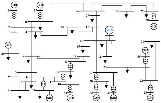
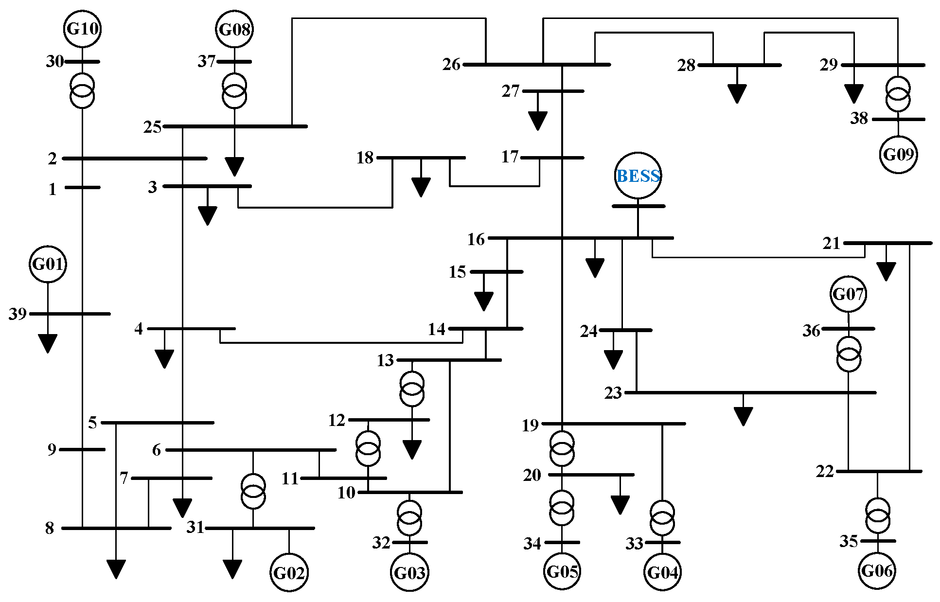
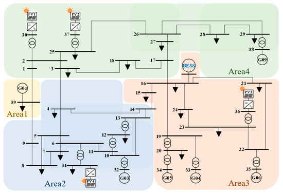
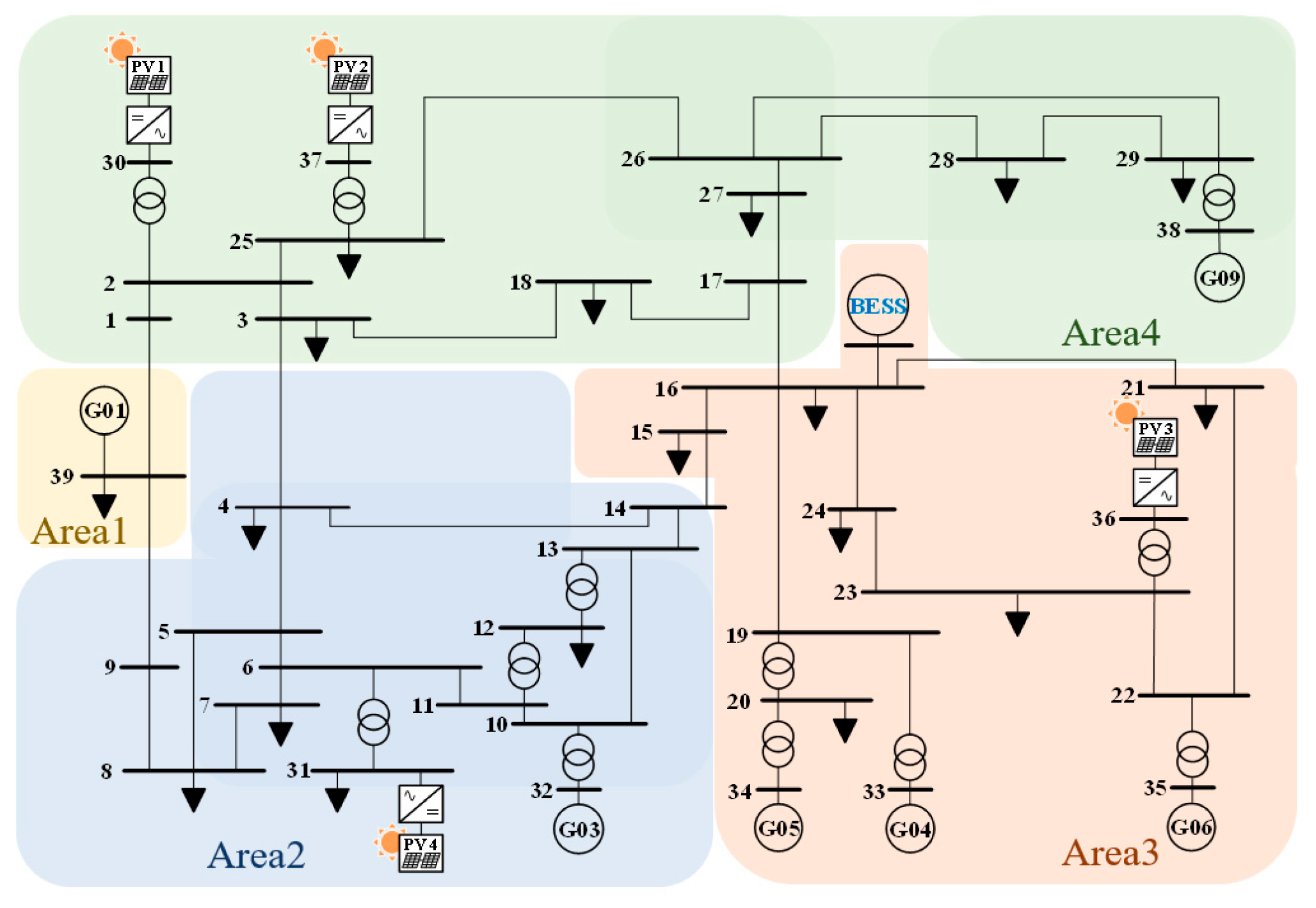
To verify the feasibility of applying the proposed inertia estimation method to a transmission-level multi-area power system, the IEEE 39-bus test system [34], whose topology is shown in Figure 7, was used as the simulation platform. This test system is a standard benchmark derived from the actual power grid in the northeastern United States. It consists of 39 buses, operates at a nominal frequency of 60 Hz, and includes 10 conventional generating units supplying a total load of 5856.8 MW. The detailed system parameters are listed in Table 1. A BESS with a rated capacity of 10 MVA is installed at Bus 16. Bus 16 is selected because it is located near the center of the system, making it a representative connection point for observing the overall system frequency response under small-signal power injection. Meanwhile, 10 MVA corresponds to approximately 0.16% of the total installed capacity of the system. An energy storage system of this scale can inject sufficient power to produce a small but measurable frequency deviation for inertia estimation, while remaining sufficiently limited so as not to dominate the overall system response or cause a large disturbance. The parameters of the BESS model are identified from real equipment data in [35] and are used to construct the small-signal injection and inertia estimation scenarios.

Figure 7. Topology of the IEEE39-bus system.

Table 1. Power system data.

Scenario	Size
Capacity	10,173.9 MVA
Generation	5913.78 MW
Loads	5856.8 MW
H	3.2 s
BESS	10 MW

4.1. System Scenarios with Different RES Penetration Levels

To evaluate the proposed method under high-RES conditions, system-wide RES penetration levels of 10%, 20%, and 30% are considered. For each case, a subset of conventional synchronous generators is replaced by inertia-less photovoltaic (PV) units to achieve the specified penetration level, as summarized in Table 2. The replacement plan is implemented cumulatively to progressively increase RES penetration: once a generator is replaced in a given case, it remains replaced in all subsequent cases, and additional synchronous generators are replaced to reach the next penetration level. For example, in Scenario 2, generators G8 and G10 are replaced; in Scenario 3, G8 and G10 remain replaced and G7 is additionally replaced; in Scenario 4, G8, G10, and G7 remain replaced and G2 is further replaced, ultimately reaching an aggregated RES penetration level of 30%. The modified IEEE 39-bus system configuration, with RES integration under the considered penetration scenarios, is shown in Figure 8. The resulting area-level penetration ratios are reported in Table 3. In addition, Table 3 lists $N_{syn}$, the number of original synchronous generators in an area, and $N_{StoR}$, the number of synchronous generators replaced by RES in an area. These statistics produce regions with low, medium, and high inertia levels and enable evaluation of the proposed method under spatially non-uniform inertia distribution.

Table 2. Settings for different RES penetration scenarios.

Scenario	Description	${\mathit{S}}_{\mathit{s}\mathit{y}\mathit{s}}$ (MVA)	${\mathit{S}}_{\mathit{s}\mathit{y}\mathit{n}}$ (MVA)	${\mathit{P}}_{\mathit{s}\mathit{y}\mathit{n}}$ (MW)	Syn to RES	${\mathit{S}}_{\mathit{R}\mathit{E}\mathit{S}}$ (MVA)	${\mathit{P}}_{\mathit{R}\mathit{E}\mathit{S}}$ (MW)	RES %	${\mathit{H}}_{\mathit{s}\mathit{y}\mathit{s}}$
1	RES 0%	10,173.9	10,173.9	5913.78	-	0	0	0	3.2
2	RES 10%		8928.7	5103.8058	G8, G10	1245.2	810	13.65	2.8
3	RES 20%		7903.7	4541.28	G7	2270.2	1370	23.17	2.4854
4	RES 30%		7067.7	3971.955	G2	3106.2	1942.93	32.84	2.2229

Figure 8. IEEE-39 bus system with integrated RES.

Table 3. Area configurations after RES replacement.

AREA	${\mathit{N}}_{\mathit{s}\mathit{y}\mathit{n}}$	${\mathit{N}}_{\mathit{S}\mathit{t}\mathit{o}\mathit{R}}$	${\mathit{H}}_{\mathit{s}\mathit{y}\mathit{n}}$	${\mathit{H}}_{\mathit{s}\mathit{y}\mathit{n}+\mathit{R}\mathit{E}\mathit{S}}$	${\mathit{S}}_{\mathit{s}\mathit{y}\mathit{n}}$ (MVA)	${\mathit{P}}_{\mathit{s}\mathit{y}\mathit{n}}$ (MW)	${\mathit{S}}_{\mathit{R}\mathit{E}\mathit{S}}$ (MVA)	${\mathit{P}}_{\mathit{R}\mathit{E}\mathit{S}}$ (MW)	RES %
2	2	1	3.2	1.607	843.7	648.719	836	572.7	49.77
3	4	3	3.2	2.448	3340.7	1786.841	1025.2	559.27	23.48
4	3	1	3.2	1.839	1684.1	829.729	1245.2	789.44	42.51

4.2. BESS Power Injection

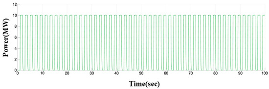
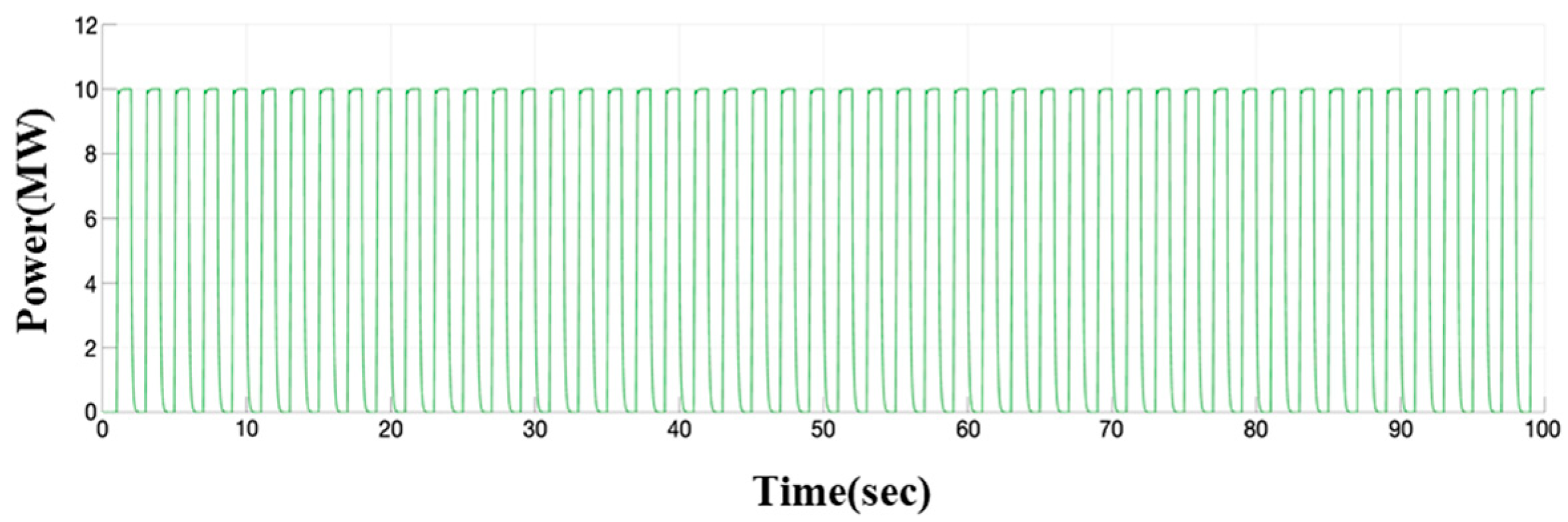
In this paper, the BESS is configured to inject a square-wave active-power signal into the power system, with a peak amplitude of 1 p.u. The test is conducted over 100 s, during which the power injection is continuously applied for 50 cycles, each with a period of 2 s. In each cycle, the BESS outputs 10 MW for the first 1 s and 0 MW for the following 1 s. As shown in Figure 9, the injected power rises to 10 MW at each rising edge and returns to 0 MW at each falling edge, forming a symmetric square-wave profile. This consistent and repeatable periodic injection serves as a controllable small-signal injection source for inertia estimation.

Figure 9. Square-wave power output of the BESS.

4.3. Frequency Observation

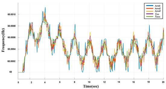
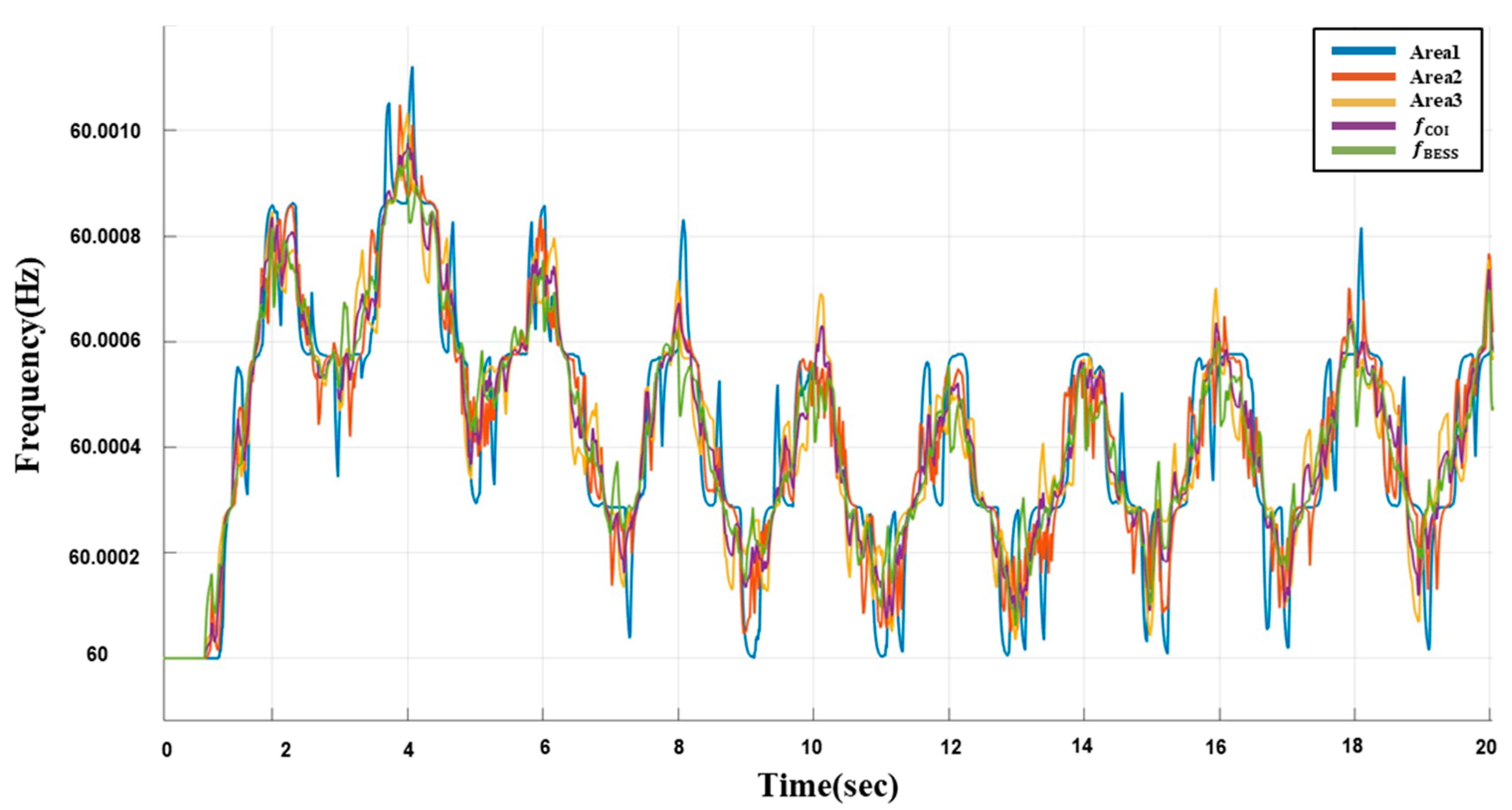
To verify that the observed frequency variations were primarily driven by the controllable small-signal power injection from the BESS, bus frequencies in different areas were monitored, emulating the deployment of PMUs in a practical power system. In addition to collecting frequency measurements at buses in multiple areas, the center-of-inertia frequency, ${\mathrm{f}}_{\mathrm{COI}}$, was also calculated. As shown in (18), ${\mathrm{f}}_{\mathrm{COI}}$ was computed as a weighted average, where ${\mathrm{H}}_{\mathrm{i}}$ and ${\mathrm{f}}_{\mathrm{i}}$ denote the inertia constant and frequency of area i, respectively, and N is the total number of areas. This formulation provides a weighted-average frequency that reflects the overall system frequency behavior [36].

$$f_{COI}={\displaystyle \frac{\sum _i^N{H}_i\cdot f_i}{{\sum }_i^N{H}_i}}$$

(18)

As shown in Figure 10, the frequency responses at different observation points are shown. The results indicate that the frequency measured at the BESS terminal, ${\mathrm{f}}_{\mathrm{BESS}}$, follows the same trend as $f_{COI}$ and the bus frequencies across the system, showing that the system frequency response is primarily driven by the injected $P_{\mathit{BESS}}$. Therefore, for inertia constant estimation, the frequency measured at the BESS terminal, ${\mathrm{f}}_{\mathrm{BESS}}$, is used as the frequency variation indicator to reduce the influence of power interactions within the system.

Figure 10. Frequency trends across multiple areas.

5. Simulations and Results

This section presents the estimation results for the original system and for systems with different RES penetration levels, along with the error statistics for each scenario.

5.1. Original System Tests

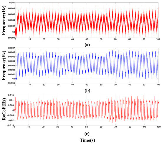
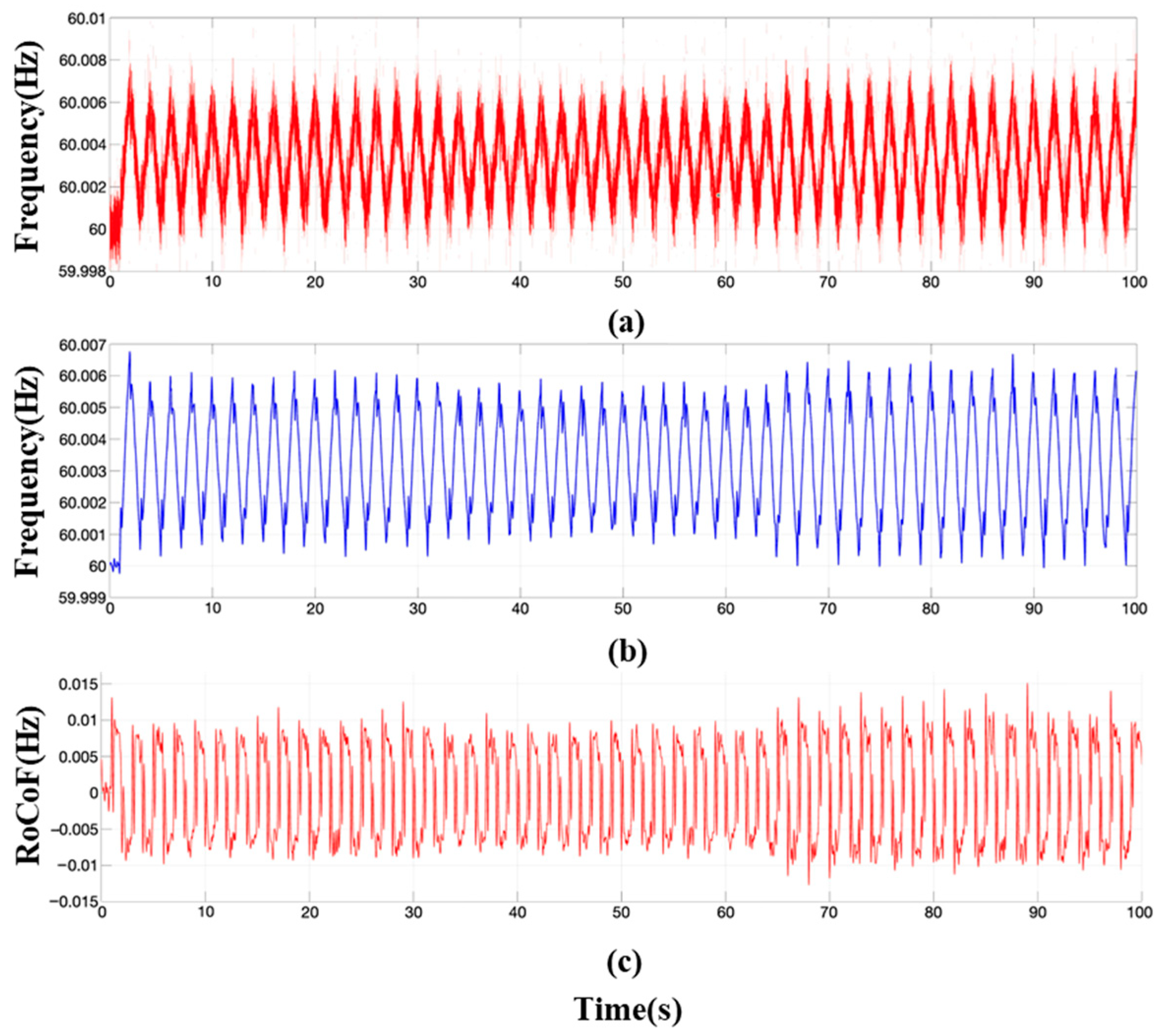
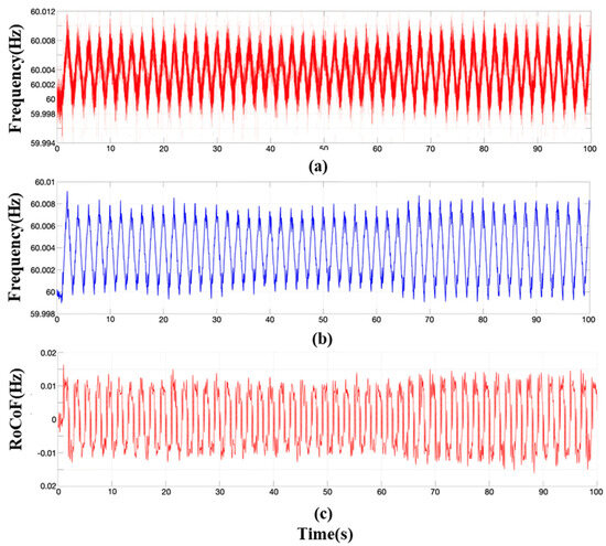
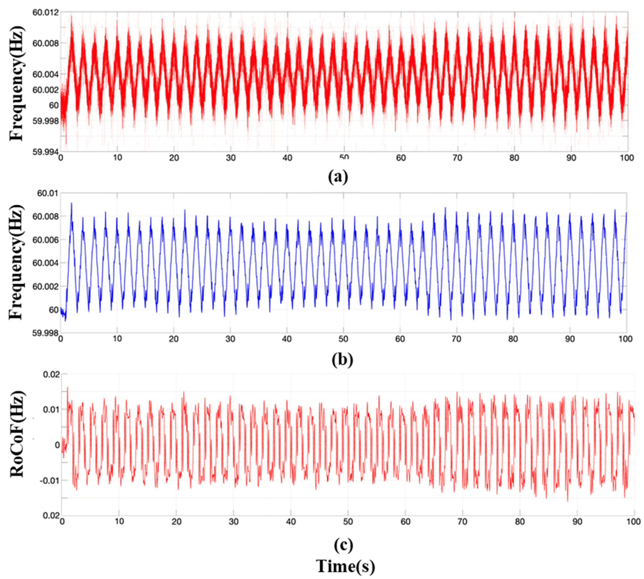
In a system composed of synchronous generators, the system inertia is provided by the synchronous machines. As shown in Figure 11a, the frequency response under a square-wave power disturbance from the BESS oscillates around 60 Hz and exhibits clear frequency deviations following each change in the storage power output. In addition, many small random spikes are superimposed on the waveform, indicating the presence of high-frequency noise. Such high-frequency components are amplified when the frequency signal is differentiated to compute the RoCoF, which degrades estimation accuracy. Therefore, signal processing is required to suppress these components. As shown in Figure 11b, the frequency response after two-stage processing using the Savitzky–Golay filter and the DWT becomes smooth and continuous, while preserving the periodic variation caused by the square-wave disturbance. The key features are retained without noticeable distortion, and the filtered signal is used as a reliable input for RoCoF calculation. By differentiating the filtered frequency signal, the RoCoF time series as shown in Figure 11c is obtained.

Figure 11. Original system (RES0%): Frequency measurements—(a) raw frequency, (b) filtered frequency, and (c) the resulting RoCoF.

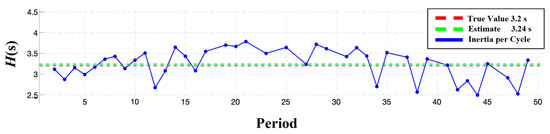
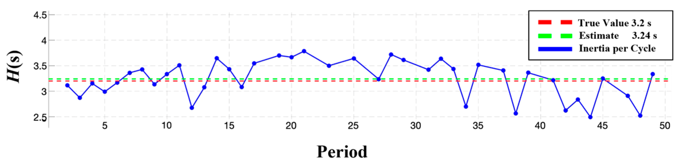
For inertia estimation, this paper uses the RoCoF extrema in each cycle as the input. A trimmed percentile approach is applied by retaining only the data within the 10th–90th percentile range; the upper and lower 10% outliers are removed, and the remaining 80% of the samples are used to compute inertia. This approach preserves the dominant dynamic response while reducing the impact of noise and outliers. As shown in Figure 12, 50 cycles are generated in this simulation; after removing the upper and lower 10% of samples, 40 valid samples are retained for analysis. The total processing time, including noise filtering and inertia estimation, does not exceed 1 min. The results show that most cycle-by-cycle estimates fall between 2.6 s and 3.7 s. The mean estimated inertia constant is 3.24 s, and the percentage error relative to the theoretical value of 3.2 s is approximately 1.26%, verifying that the proposed method achieves acceptable estimation accuracy under the studied system conditions.

Figure 12. Original system (RES0%) inertia estimation results.

5.2. Testing on a RES-Integrated Power System

For all scenarios, the measured frequency data are processed using the same signal-processing procedure described earlier, including the two-stage filtering and the RoCoF calculation based on a sliding window, to extract key features required for inertia estimation. After replacing synchronous generators with RESs, the overall system inertia decreases because these resources are non-inertial. For RES penetration levels of 10%, 20%, and 30%, the inertia constant $H_{sys}$ decreases from 3.2 to 2.808, 2.485, and 2.223, respectively. As shown in Figure 13a–c, the frequency response and RoCoF under the 30% RES penetration scenario are driven by the BESS output. Due to the reduced inertia, the same BESS output leads to larger variations in both the frequency response and RoCoF.

Figure 13. RES30% system: Frequency measurements—(a) raw frequency, (b) filtered frequency, and (c) the resulting RoCoF.

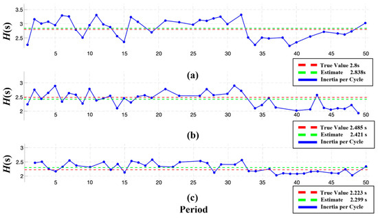
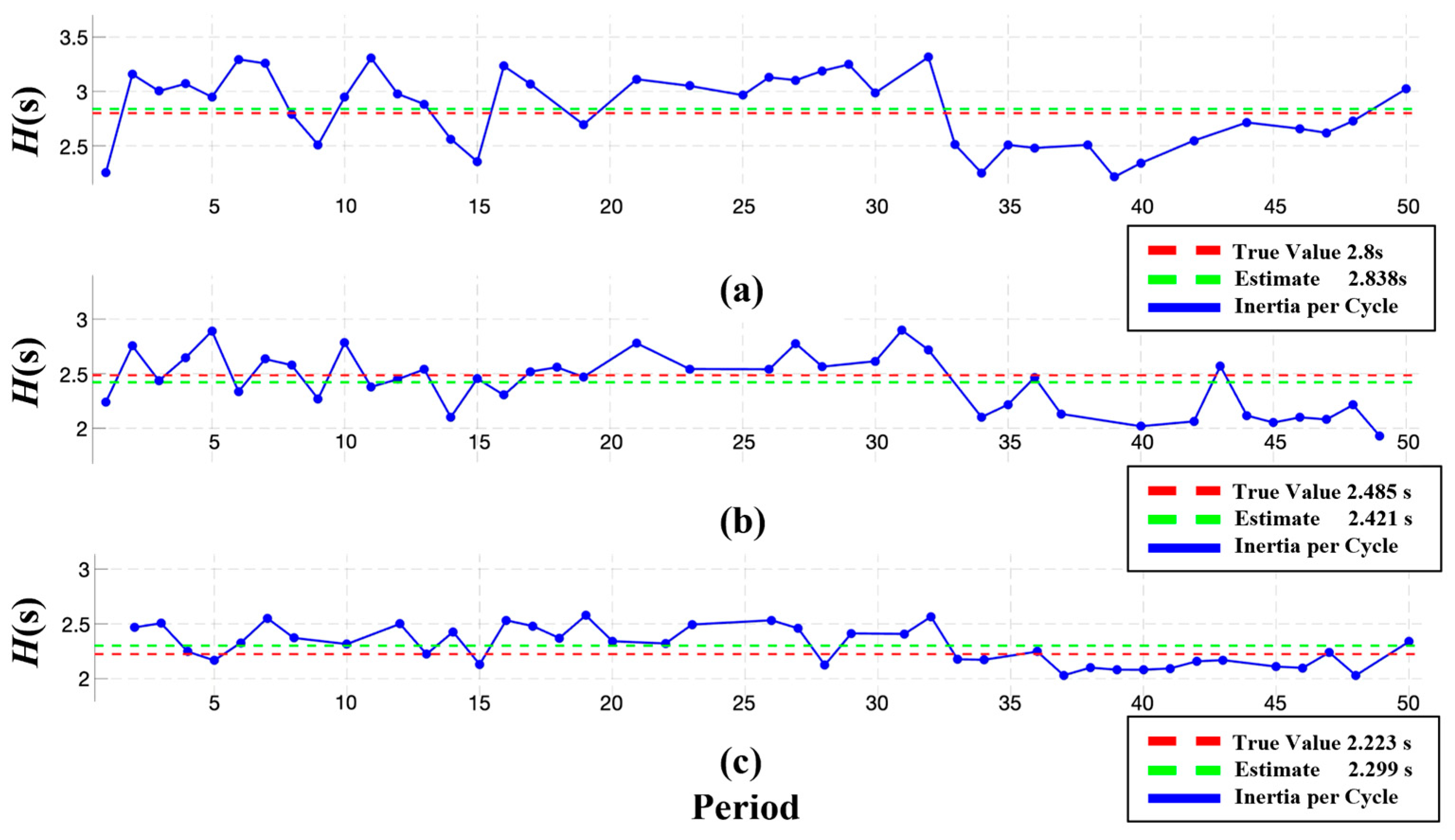
The comparison between the estimated inertia $H_{est}$ and the corresponding system inertia $H_{sys}$ for each scenario is shown in Figure 14a–c. In the RES10% scenario, most $H_{est}$ values fall within 2.4–3.3 s. After outlier screening, the estimated mean is 2.838 s, corresponding to an error of approximately 1.35% relative to $H_{sys}$ 2.8 s. In the RES20% scenario, most $H_{est}$ values fall within 2.0–2.9 s. After outlier screening, the estimated mean is 2.421 s, yielding an error of approximately 2.6% compared with $H_{sys}$ 2.485 s. In the RES30% scenario, most $H_{est}$ values fall within 2.0–2.6 s. After outlier screening, the estimated mean is 2.299 s, resulting in an error of approximately 3.4% relative to $H_{sys}$ 2.223 s. Even under high-RES penetration, where the system rotational kinetic energy is significantly reduced, the proposed method maintains acceptable estimation accuracy.

Figure 14. Inertia estimation results: (a) RES10%, (b) RES20%, and (c) RES30%.

5.3. Error Trend and Statistical Analysis

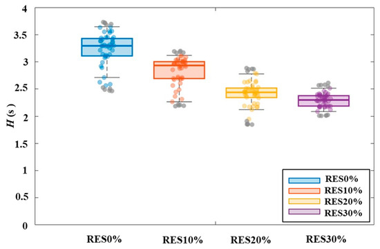
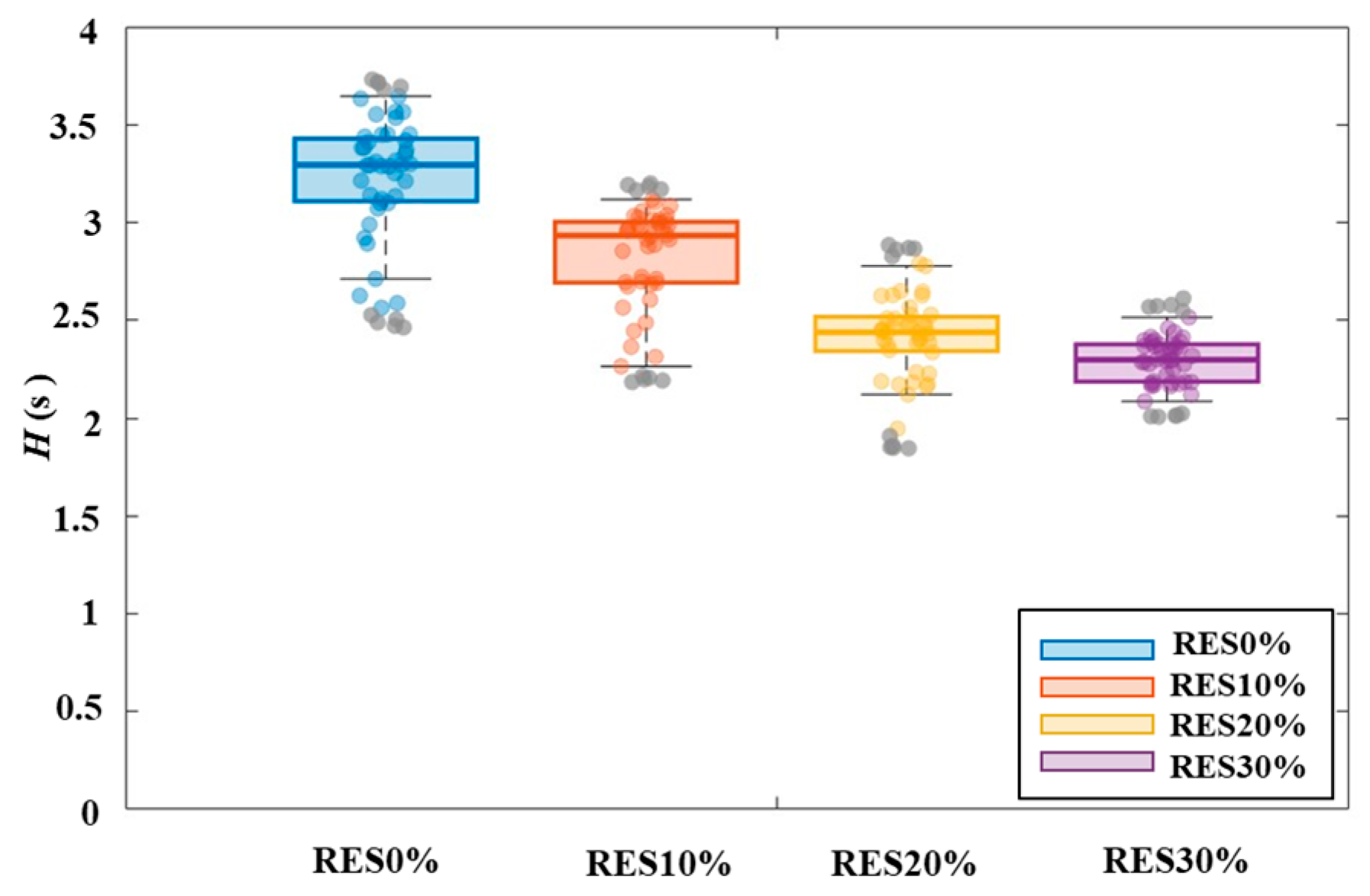
By analyzing and comparing the simulation results, the estimation accuracy and general applicability of the proposed method can be evaluated. As shown in Figure 15, the $H_{est}$ values are computed for each disturbance cycle under all scenarios. The colored markers indicate the samples retained for the boxplot statistics, whereas the gray markers denote the extreme values removed by the upper and lower 10% trimming. From RES0% to RES30%, the range between the maximum and minimum $H_{est}$ decreases from approximately 1.1 s to 0.6 s. For the RES30% scenario, $H_{sys}$ is 2.22 s and $H_{est}$ is mainly distributed within 2.0–2.6 s, with a mean of 2.229 s and a median of 2.298 s. Under reduced inertia, the same BESS output leads to a larger RoCoF, which is consistent with the progressive reduction in system inertia as RES penetration increases. Moreover, because reduced inertia amplifies the RoCoF and frequency variations under the same disturbance, the identification features become more pronounced relative to measurement noise. Consequently, with the same signal-processing and sliding-window settings, the dispersion of $H_{est}$ decreases, and the estimates exhibit a more concentrated distribution.

Figure 15. Statistics of estimated inertia under different scenarios.

At this stage, the percentage error PE% and the mean-difference metric $e$ are calculated for each scenario, where $e$ =$H_{sys}$ − $H_{est}$. Table 4 summarizes the values of $H_{sys}$, $H_{est}$, the median, PE% and $e$ for all scenarios. The results show that both PE% and $e$ gradually increase from RES0% to RES30%. indicating that the estimation becomes more sensitive as system inertia decreases. This trend is consistent with the reduction in $H_{sys}$ caused by the increasing penetration of non-inertial RESs without virtual inertia support. Under low-inertia conditions, the same absolute deviation ∣$H_{sys}$ − $H_{est}$∣ leads to a larger relative error in terms of PE%, highlighting the increased importance of estimation accuracy as RES penetration rises.

Table 4. Summary of inertia estimation and error metrics.

Scenario	${\mathit{H}}_{\mathit{s}\mathit{y}\mathit{s}}$	$\overline{{\mathit{H}}_{\mathit{e}\mathit{s}\mathit{t}}}$	Median	PE%	$\mathit{e}$
RES 0%	3.2	3.2403	3.294	1.26	0.0403
RES 10%	2.8	2.8377	2.933	1.35	0.0377
RES 20%	2.485	2.4206	2.43	2.57	0.0639
RES 30%	2.223	2.2992	2.298	3.43	0.0763

Overall, the proposed framework maintains the estimation error within an acceptable range across all studied RES penetration scenarios. Although the error gradually increases as RES penetration rises and the equivalent system inertia decreases, the estimated inertia still follows the theoretical trend well, indicating that the framework can reliably capture inertia variations under different operating conditions. These results demonstrate that the proposed framework provides stable and accurate estimation performance not only in relatively high-inertia cases but also in low-inertia conditions with higher RES penetration. The consistent performance across RES0% to RES30% confirms the robustness of the framework against changing system inertia levels and measurement noise.

From an application perspective, the proposed framework has potential value for real-time inertia monitoring and operational assessment in transmission-level power systems with high-RES penetration. Because the framework does not rely on major disturbance events and instead uses controllable small-signal power injection from a BESS, it can support continuous awareness of system inertia under normal operating conditions. This capability may be useful for online security assessment, operational planning, and stability-oriented control support in future low-inertia power systems, where timely knowledge of inertia variations is increasingly important.

6. Conclusions

This paper proposes a BESS-based continuous inertia estimation framework for transmission-level power systems with high renewable energy source (RES) penetration. The proposed framework combines controllable small-signal power injection, two-stage signal processing, and moving-window RoCoF analysis to improve estimation robustness under noisy measurement conditions. Validation on the IEEE 39-bus system under RES penetration levels of 0%, 10%, 20%, and 30% shows that the estimation error remains within ±3.5% across all scenarios, ranging from 1.26% at 0% RES penetration to 3.43% at 30% RES penetration. These results confirm that the proposed framework can provide accurate and stable inertia estimation under low-inertia, high-RES operating conditions, making it suitable for real-time inertia monitoring and operational assessment in future power systems with high RES penetration.

References

- Lavanya, L.; Swarup, K.S. Inertia monitoring in powersystems: Critical features, challenges, and framework. Renew. Sustain. Energy Rev. 2024, 190, 114076. [Google Scholar]
- Prabhakar, K.; Jain, S.K.; Padhy, P.K. Inertia estimation in modern power system: A comprehensive review. Electr. Power Syst. Res. 2022, 211, 108222. [Google Scholar] [CrossRef] [Scilit]
- Tan, B.; Zhao, J.; Netto, M.; Krishnan, V.; Terzija, V.; Zhang, Y. Power system inertia estimation: Review of methods and the impacts of converter-interfaced generations. Int. J. Electr. Power Energy Syst. 2022, 134, 107362. [Google Scholar] [CrossRef] [Scilit]
- Heidari, M.; Ding, L.; Kheshti, M.; Bao, W.; Zhao, X.; Popov, M.; Terzija, V. A review on application of machine learning-based methods for power system inertia monitoring. Int. J. Electr. Power Energy Syst. 2024, 162, 110279. [Google Scholar] [CrossRef] [Scilit]
- Abouyehia, M.; Egea-Alvarez, A.; Ahmed, K.H. Evaluating inertia estimation methods in low-inertia power systems: A comprehensive review with analytic hierarchy process-based ranking. Renew. Sustain. Energy Rev. 2025, 217, 115794. [Google Scholar] [CrossRef] [Scilit]
- Hadavi, A.; Hagh, M.T.; Zadeh, S.G. Critical inertia thresholds for frequency stability in renewable Energy-Integrated power systems. Int. J. Electr. Power Energy Syst. 2025, 169, 110733. [Google Scholar] [CrossRef] [Scilit]
- Zhang, W.; Wen, Y.; Chung, C.Y. Inertia security evaluation and application in low-inertia power systems. IEEE Trans. Power Syst. 2025, 40, 1725–1737. [Google Scholar] [CrossRef] [Scilit]
- Inoue, T.; Taniguchi, H.; Ikeguchi, Y.; Yoshida, K. Estimation of power system inertia constant and capacity of spinning-reserve support generators using measured frequency transients. IEEE Trans. Power Syst. 1997, 12, 136–143. [Google Scholar] [CrossRef] [Scilit]
- Bian, Y.; Wyman-Pain, H.; Li, F.; Bhakar, R.; Mishra, S.; Padhy, N.P. Demand Side Contributions for System Inertia in the GB Power System. IEEE Trans. Power Syst. 2018, 33, 3521–3530. [Google Scholar] [CrossRef] [Scilit]
- Ashton, P.M.; Saunders, C.S.; Taylor, G.A.; Carter, A.M.; Bradley, M.E. Inertia Estimation of the GB Power System Using Synchrophasor Measurements. IEEE Trans. Power Syst. 2015, 30, 701–709. [Google Scholar] [CrossRef] [Scilit]
- Wang, Y.; Yokoyama, A.; Baba, J. A Multifunctional Online Estimation Method for Synchronous Inertia of Power Systems Using Short-Time Phasor Transient Measurement Data with Linear Least Square Method After Disturbance. IEEE Access 2024, 12, 17010–17022. [Google Scholar] [CrossRef] [Scilit]
- Kerdphol, T.; Watanabe, M.; Mitani, Y.; Ngamroo, I. Inertia Assessment from Transient Measurements: Recent Perspective from Japanese WAMS. IEEE Access 2022, 10, 66332–66344. [Google Scholar] [CrossRef] [Scilit]
- Tuttelberg, K.; Kilter, J.; Wilson, D.; Uhlen, K. Estimation of Power System Inertia from Ambient Wide Area Measurements. IEEE Trans. Power Syst. 2018, 33, 7249–7257. [Google Scholar] [CrossRef] [Scilit]
- Zeng, F.; Zhang, J.; Chen, G.; Wu, Z.; Huang, S.; Liang, Y. Online Estimation of Power System Inertia Constant Under Normal Operating Conditions. IEEE Access 2020, 8, 101426–101436. [Google Scholar] [CrossRef] [Scilit]
- Li, H.; You, S.; Jiang, Z.; Tan, J.; Hoke, A.; Liu, J.; Zhu, L.; Rockwell, B.; Kruse, C.; Liu, Y. Ambient-Frequency-Data Based System-Level Inertia Estimation Using Physical Equation and its Practice on Hawaii Islands. IEEE Trans. Power Syst. 2024, 39, 6948–6959. [Google Scholar] [CrossRef] [Scilit]
- Yang, D.; Wang, B.; Ma, J.; Chen, Z.; Cai, G.; Sun, Z.; Wang, L. Ambient-Data-Driven Modal-Identification-Based Approach to Estimate the Inertia of an Interconnected Power System. IEEE Access 2020, 8, 118799–118807. [Google Scholar] [CrossRef] [Scilit]
- Bi, T.; Liu, J.; Wang, C. Online Estimation of Area-Level Inertia Considering Inter-Area Equivalent Frequency Dynamics. IEEE Trans. Power Syst. 2025, 40, 57–72. [Google Scholar] [CrossRef] [Scilit]
- Azizi, S.; Sun, M.; Liu, G.; Terzija, V. Local Frequency-Based Estimation of the Rate of Change of Frequency of the Center of Inertia. IEEE Trans. Power Syst. 2020, 35, 4948–4951. [Google Scholar] [CrossRef] [Scilit]
- Kerdphol, T.; Watanabe, M.; Nishikawa, R.; Hayashi, Y.; Mitani, Y. Inertia Estimation of the 60 Hz Japanese Power System from Synchrophasor Measurements. IEEE Trans. Power Syst. 2023, 38, 753–766. [Google Scholar] [CrossRef] [Scilit]
- AEMO. Quantifying Synthetic Inertia of a Grid-Forming Battery Energy Storage System—Technical Note; Technical Note (Version 1.0); AEMO: Melbourne, Australia, 2024. [Google Scholar]
- Tamrakar, U.; Copp, D.A.; Nguyen, T.A.; Hansen, T.M.; Tonkoski, R. Real-Time Estimation of Microgrid Inertia and Damping Constant. IEEE Access 2021, 9, 114523–114534. [Google Scholar] [CrossRef] [Scilit]
- Hosaka, N.; Berry, B.; Miyazaki, S. The world’s first small power modulation injection approach for inertia estimation and demonstration in the island grid. In Proceedings of the 2019 8th International Conference on Renewable Energy Research and Applications (ICRERA), Brașov, Romania, 3–6 November 2019; pp. 722–726. [Google Scholar]
- Anderson, P.M.; Fouad, A.A. Power System Control and Stability, 2nd ed.; Wiley-IEEE Press: Hoboken, NJ, USA, 2002. [Google Scholar]
- Zhang, J.; Tang, L.; Mingotti, A.; Peretto, L.; Wen, H. Analysis of White Noise on Power Frequency Estimation by DFT-Based Frequency Shifting and Filtering Algorithm. IEEE Trans. Instrum. Meas. 2020, 69, 4125–4133. [Google Scholar] [CrossRef] [Scilit]
- Yang, P.; Tan, Z.; Wiesel, A.; Nehorai, A. Power System State Estimation Using PMUs With Imperfect Synchronization. IEEE Trans. Power Syst. 2013, 28, 4162–4172. [Google Scholar] [CrossRef] [Scilit]
- John, A.; Sadasivan, J.; Seelamantula, C.S. Adaptive Savitzky-Golay Filtering in Non-Gaussian Noise. IEEE Trans. Signal Process. 2021, 69, 5021–5036. [Google Scholar] [CrossRef] [Scilit]
- Krishnan, S.R.; Seelamantula, C.S. On the Selection of Optimum Savitzky-Golay Filters. IEEE Trans. Signal Process. 2013, 61, 380–391. [Google Scholar] [CrossRef] [Scilit]
- Grande, L.S.A.; Granizo, R.; Arnaltes, S. Wavelet analysis to detect ground faults in electrical power systems with full penetration of converter interface generation. Electronics 2023, 12, 1085. [Google Scholar] [CrossRef] [Scilit]
- Avdaković, S.; Nuhanović, A.; Kusljugić, M. Wavelets as a tool for power system dynamic events analysis. J. King Saud Univ.—Eng. Sci. 2017, 29, 258–269. [Google Scholar]
- Guo, Y.; Zhou, X.; Li, J.; Ba, R.; Xu, Z.; Tu, S.; Chai, L. A Novel and Optimized Sine–Cosine Transform Wavelet Threshold Denoising Method Based on the sym4 Basis Function and Adaptive Threshold Related to Noise Intensity. Appl. Sci. 2023, 13, 10789. [Google Scholar] [CrossRef] [Scilit]
- Ten, C.F.; Crossley, P.A. Evaluation of RoCoF relay performances on networks with distributed generation. In Proceedings of the CIRED 2005—18th International Conference Electricity Distribution, Turin, Italy, 6–9 June 2005; pp. 1–4. [Google Scholar]
- Rezkalla, M.; Pertl, M.; Marinelli, M. Electric power system inertia: Requirements, challenges and solutions. Electr. Eng. 2018, 100, 1983–2002. [Google Scholar] [CrossRef] [Scilit]
- Yin, H.; Qiu, W.; Wu, Y.; You, S.; Tan, J.; Hoke, A.; Kruse, C.J.; Rockwell, B.W.; Liu, Y. Field measurement and analysis of frequency and RoCoF for low-inertia power systems. IEEE Trans. Ind. Electron. 2024, 71, 7996–8006. [Google Scholar] [CrossRef] [Scilit]
- Athay, T.; Podmore, R.; Virmani, S. A Practical Method for the Direct Analysis of Transient Stability. IEEE Trans. Power Appar. Syst. 1979, 98, 573–584. [Google Scholar] [CrossRef] [Scilit]
- Chang, C.-M.; Chang, H.-C.; Hung, C.-C.; Kuo, C.-C. The Impact of Energy Storage System Control Parameters on Frequency Regulation Strategies. IEEE Access 2025, 13, 34010–34022. [Google Scholar] [CrossRef] [Scilit]
- You, S.; Li, H.; Liu, S.; Sun, K.; Wang, W.; Qiu, W.; Liu, Y. Calculate center-of-inertia frequency and system RoCoF using PMU data. In Proceedings of the IEEE Power & Energy Society General Meeting (PESGM), Washington, DC, USA, 26–29 July 2021; pp. 1–5. [Google Scholar]
Disclaimer/Publisher’s Note: The statements, opinions and data contained in all publications are solely those of the individual author(s) and contributor(s) and not of MDPI and/or the editor(s). MDPI and/or the editor(s) disclaim responsibility for any injury to people or property resulting from any ideas, methods, instructions or products referred to in the content. |
© 2026 by the authors. Licensee MDPI, Basel, Switzerland. This article is an open access article distributed under the terms and conditions of the Creative Commons Attribution (CC BY) license.