Feasibility of Applying Kriging for Earthquake Ground Motion Intensity Measures in South Korea

Abstract

Estimating ground motion parameters at an unsampled site is challenging for seismologists and engineers alike. An attempt is made to apply Kriging interpolation to estimate peak ground accelerations at specific nuclear power plant sites. However, issues such as data quality and Kriging assumptions pose challenges to how practical and reasonable Kriging interpolation results may be in terms of estimating ground motion parameters. Peak ground acceleration data from the 2016 Gyeongju and 2017 Pohang earthquakes were taken from a local seismological agency. Peak ground acceleration, logarithms of the peak ground acceleration, and residuals between the recorded data and global and local ground motion models were used to select and derive empirical variogram models. The leave-one-out cross-validation process suggested estimating peak ground acceleration residuals from a locally developed ground motion model using an Exponential variogram model. Kriging estimates were compared to a site-specific ground motion model. These estimates appeared reasonable at one site but were significantly off at the other site. On the whole, Kriging estimates were lower than ground motion model predictions. When viewed relative to the nearest recordings, Kriging estimates appeared inconsistent across the two earthquake events. A nearest neighbor approach to computing Kriging estimates suggested a minimum of five data points but much more for modeling an empirical variogram. Results also suggest focusing on validation processes more than variogram selection. This suggests caution when applying Kriging for ground motion-related assessments in South Korea.

1. Introduction

An interest in seismology and earthquake hazard studies has been renewed in the Korean peninsula, primarily due to the 2016 M_W 5.5 Gyeongju and 2017 M_W 5.5 Pohang earthquakes. These moderately sized earthquakes occurred near multiple nuclear power plant (NPP) complexes and an underground radioactive waste repository [1,2]. Such events made the populace re-evaluate emergency preparedness and hazard studies, as well as the understanding of the seismological environment of South Korea.

An important issue during this seismic rejuvenation is the estimation of earthquake ground motion shaking levels, especially in areas where there is no ground motion instrumentation. A family of methods in estimating parameters at different locations is Kriging interpolation, more commonly known as just Kriging. Kriging is a geostatistical technique based on the premise that values of a variable at nearby locations tend to be more similar than values at distant locations [3,4,5,6]. This premise is more commonly known as spatial correlation. Several studies have applied Kriging interpolation methods in estimating earthquake ground shaking and related matters.

Two studies demonstrated the development of ground shaking contours for well-documented earthquakes in California, USA [7,8]. Of these, one study applied Kriging directly to peak values [7], while the other transformed the peak values into a probability [8]. These studies showed differences in contours from ground motion models as well as different types of Kriging, noting that the ground motion models (GMMs) they applied tended to overestimate intensity measures or that Kriging estimates tended to be underestimated. Another study in Japan utilized boring-derived information to improve Kriging estimates used for developing contours [9]. Interestingly, Kriging is frequently used for contour development in modern practice. Kriging was also used to develop related contours for earthquake intensity in Italy and Costa Rica [10,11]. Naturally, these studies had sizable, well-studied data sets; supposedly, a necessary condition for performing a useful Kriging (>>30) [12,13,14]. Kriging has also been utilized in estimating factors that affect ground motion shaking, such as the time average shear wave velocity in the upper 30 m of material [15,16,17,18], while other studies expand the application of Kriging to generate data to estimate structural response parameters in uninstrumented infrastructure from earthquake ground shaking [19,20,21].

Many of these studies appeared to apply variogram models that did not seem to fit the data evenly, had significant scatter, or only provided variogram model parameters [7,8,9,10,11,18,19,20]. Likewise, several of these studies do not show verification or validation, with a few implying it is somewhat difficult with small data sets.

As such, this study attempts to perform Kriging and validation to estimate earthquake ground motions at two sites utilizing a small data set (<30). Due to data availability, only peak ground accelerations (PGAs) from digitally recorded ground motions are considered herein. Cross validation is conducted, in addition to other related metrics, to gauge the performance of the model variogram and internal Kriging estimates. Then after, Kriging is applied to estimate the logarithm of the PGA, the intra-event residuals from a Global GMM, and the intra-event residuals from a locally derived GMM for two earthquake events at two NPP sites. These two NPP sites were selected not only because of local interest but also due to the existence of a unique site-specific GMM designed for South Korean NPP sites. Unlike most GMMs, this site-specific GMM accounts for local site and path effects with extensive verification procedures [22]. Furthermore, this study expands on the Kriging estimates by examining the premise of spatial correlation in applying a nearest-neighbor approach in Kriging estimates; that is, if closer sites are more correlated than further sites, then would using only closer sites in Kriging interpolation produce a better estimate? It is expected that, as the number of further sites is reduced, Kriging estimates will approach the site-specific GMM estimates. This study assumes the data are isotropic and, in certain cases, satisfying assumptions behind empirical variogram modeling. This study also assumes surficial distance estimates are accurate representations without loss of pertinent information. Hopefully, the results of this study will help extend the database on Kriging with smaller data sets in performance assessments and in determining which areas can or should be invested in to help improve the work of engineers, modelers, and policy makers.

2. Materials and Methods

Descriptions on available data, Kriging implementation, and adjustments to data are made here. Kriging is split into two parts, with the selection of an appropriate variogram and derivation of Kriging weights for interpolation at unsampled points. These parts will be detailed in sequence.

2.1. Data Source

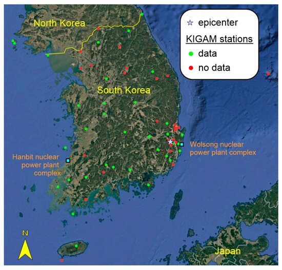
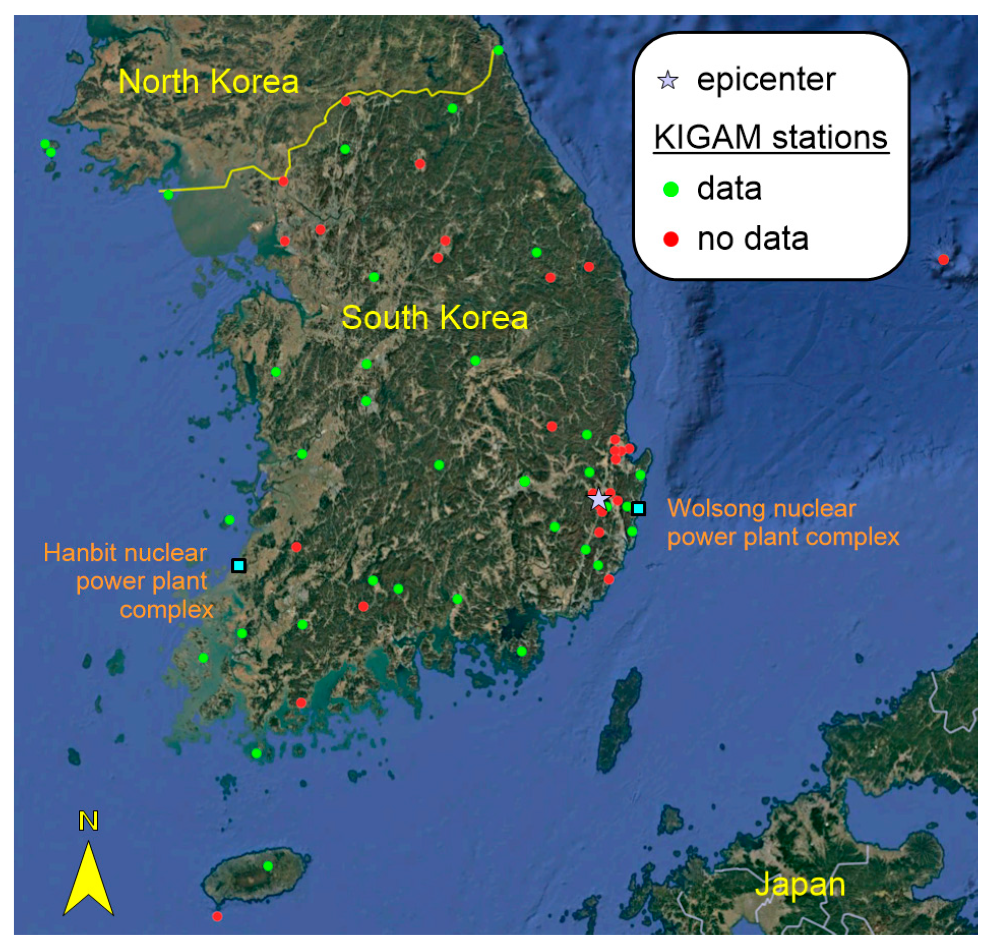
Only data provided by Korea Institute of Geoscience and Mineral Resources (KIGAM) is considered. KIGAM has an active nationwide seismic observatory network with site information and relatively good support [23]. For practicality, PGAs from the 2016 M_W 5.5 M_L 5.8 Gyeongju earthquake and 2017 M_W 5.5 M_L 5.4 Pohang earthquakes are used [1,2]. For the Gyeongju earthquake, 34 KIGAM seismic observatories have a recorded PGA available. Figure 1 shows the distribution of the KIGAM seismic observatories that recorded a PGA for the Gyeongju earthquake. However, only 24 of these stations are installed on the surface and were actively operational during the earthquake. For the Pohang earthquake, 27 surface-installed stations have a recorded PGA. Note that the Pohang earthquake epicenter is approximately 40 km northeast of the 2016 Gyeongju event, and although it is from the same seismically active region, it is generally considered an anthropogenic event. Active stations during the earthquake are shown in Table 1. As expected, stations closer to the epicenter recorded higher PGAs, and stations farther from the epicenter recorded relatively lower PGAs, typically below 1 cm/s², which is quite small.

Figure 1. Seismic observatories operated by KIGAM. Green symbols represent stations which have processed recordings of the 2016 Gyeongju earthquake. Epicenter of the 2016 Gyeongju earthquake is marked with a purple star. Hanbit and Wolsong NPP complexes are also located in blue squares.

Table 1. Seismic stations where KIGAM posted a PGA value. Seismic stations are represented by a station code with their corresponding location listed.

			2016 Gyeongju Earthquake [1]		2017 Pohang Earthquake [2]
Station Code	Latitude (°)	Longitude (°)	Epicentral Distance (km)	PGA (cm/s2)	Epicentral Distance (km)	PGA (cm/s2)
AJD	34.75	126.12	300.8	1.04	331.2	0.75
BBK	35.58	129.44	29.9	52.16	59.1	5.69
BGD	34.16	126.56	299.0	1.42	335.5	0.47
BRN	37.97	124.64	474.4	0.90	469.1	0.29
BRS	37.92	124.69	467.3	0.55	462.2	0.21
CGD	35.61	128.84	35.7	60.52	73.3	5.28
CHS	36.18	129.09	47.6	18.04	26.6	21.46
DKJ	35.95	129.11	22.0	80.82	29.7	44.89
GKP1	35.89	128.61	54.7	43.53	73.1	13.74
GRE	35.26	127.44	167.9	3.35	198.2	2.68
HAK	35.93	129.50	33.8	19.43	23.2	34.12
HKU	36.61	127.36	190.0	9.98	189.0	4.30
KJM	34.83	128.59	116.2	7.82	158.2	2.63
KMC	35.99	127.94	115.4	7.23	129.3	6.33
KSA	38.60	128.35	323.4	0.59	290.2	0.90
MAK	35.37	129.18	43.3	38.30	83.9	3.42
MKL	35.73	129.24	5.6	227.10	43.5	9.72
MRD	33.12	126.27			437.3	0.35
MUN	34.91	126.43	268.3	1.34	298.4	0.80
NPR	36.04	126.87	212.1	5.32	225.6	2.12
PCH	37.96	127.13	305.8	0.81	286.3	0.67
SND	37.16	128.80			127.1	6.44
SNU	37.45	126.95			262.1	1.53
TJN	36.38	127.36	178.5	5.65	183.0	2.90
WID	35.62	126.31	261.5	1.97	282.0	0.94
YIN	37.16	127.40	223.3	1.98	211.2	2.50
YPD	37.66	125.70	376.5	0.79	369.7	0.47

2.2. Kriging Estimator

Kriging is a multi-stage geostatistical method and is briefly introduced here. Kriging is the common name given to a set of methods revolving around spatial interpolation [3,4,5,6]. Spatial samples are treated as:

$$Z\left(u\right)=\mu \left(u\right)+\epsilon \left(u\right)$$

(1)

where $Z\left(u\right)$ is the value of the variable of interest at location $u$, $\mu \left(u\right)$ is a location-dependent mean, and the random variable $\epsilon \left(u\right)$ is a zero mean second-order stationary random field with a covariance function $C\left(h\right)$ and variogram $\gamma \left(h\right)$, where $h$ is lag. Lag, in geostatistics, is treated as the distance between sample locations $u$. Therefore, the distance between location $u_1$ and $u_2$ is the lag. Note that for a covariance at 0 distance, $C\left(0\right)$ is the variance. The correlation between mean and residual is assumed to be 0. With this nomenclature, the Ordinary Kriging estimator is typically denoted as:

$$Z^{\ast }\left(u_0\right)=\sum _{i=1}^{n}w\left(u_i\right)Z\left(u_i\right)$$

(2)

where $Z^{\ast }\left(u_0\right)$ is the estimated value at interested location $u_0$, $i$ is an index for sampled values up to a limit of $n$ sampled neighbors, $w$ is a regressed weight, and $Z\left(u_i\right)$ are known values at sampled locations $u_i$. The weights are estimated by minimizing the expected square of the estimation error from Equation (2):

$$e=E{\left[Z^{\ast }\left(u_0\right)-\sum _{i=1}^n{w}_{i}Z\left(u_i\right)\right]}^2$$

(3)

where subject to an unbiasedness constraint, $\sum w_i=1$. Inclusion of the unbiasedness constraint is commonly denoted as Ordinary Kriging. Incorporating an optimization technique known as the Lagragian multiplier method to account for the unbiasedness constraint leads to a set of normal equations:

$$\left[\begin{array}{ccc}\begin{array}{cc}{\gamma }_{11}& {\gamma }_{12}\\ {\gamma }_{21}& {\gamma }_{22}\end{array}& \dots & \begin{array}{cc}{\gamma }_{1m}& 1\\ {\gamma }_{2m}& 1\end{array}\\ ⋮& \ddots & ⋮\\ \begin{array}{cc}{\gamma }_{m1}& {\gamma }_{m2}\\ 1& 1\end{array}& \dots & \begin{array}{cc}{\gamma }_{mm}& 1\\ 1& 0\end{array}\end{array}\right]\left[\begin{array}{c}{w}_1\\ w_2\\ \begin{array}{c}⋮\\ w_m\\ \lambda \end{array}\end{array}\right]=\left[\begin{array}{c}{\gamma }_{01}\\ {\gamma }_{02}\\ \begin{array}{c}⋮\\ {\gamma }_{0m}\\ 1\end{array}\end{array}\right]$$

(4)

where ${\gamma }_{ij}$ is the aforementioned variogram, representing the contrast between location $i$ and $j$, equivalent to $\gamma \left(u_i,u_j\right)$. Again, the aforementioned lag $h$ is the distance between locations indexed by $i$ and $j$. A solution for the vector of weights can be determined by inverting the variogram matrix of sampled locations:

$$\left[\begin{array}{c}{w}_1\\ w_2\\ \begin{array}{c}⋮\\ w_m\\ \lambda \end{array}\end{array}\right]={\left[\begin{array}{ccc}\begin{array}{cc}{\gamma }_{11}& {\gamma }_{12}\\ {\gamma }_{21}& {\gamma }_{22}\end{array}& \dots & \begin{array}{cc}{\gamma }_{1m}& 1\\ {\gamma }_{2m}& 1\end{array}\\ ⋮& \ddots & ⋮\\ \begin{array}{cc}{\gamma }_{m1}& {\gamma }_{m2}\\ 1& 1\end{array}& \dots & \begin{array}{cc}{\gamma }_{mm}& 1\\ 1& 0\end{array}\end{array}\right]}^{-1}\left[\begin{array}{c}{\gamma }_{01}\\ {\gamma }_{02}\\ \begin{array}{c}⋮\\ {\gamma }_{0m}\\ 1\end{array}\end{array}\right]$$

(5)

These weights are also used to estimate the variance of the Kriging error. From the same principles as mentioned above, manipulation of Equation (3), and the weights from Equation (5), the resultant error variance is:

$${\sigma }^2\left(u_0\right)=C\left(0\right)-\sum _{i=1}^{n}w\left(u_i\right)\gamma \left(u_0,u_i\right)-\lambda$$

(6)

which is essentially the difference between the variance and the Kriging weighted variogram values relative to the target site. Note how Equation (6) does not depend on sampled values. Ordinary Kriging interpolation techniques were derived assuming the geospatial data satisfies second order stationarity, i.e., constant mean and variance depending on lag. Interestingly, geospatially observed data cannot be used to directly check for geospatial stationarity. This assumption allows the use of a variogram to model the observed data.

2.3. Variogram

The variogram is a key component in Kriging. A variogram is a function that describes the spatial variability of the sampled data as a function of distance and/or direction. Typically, spatial data is used to derive an empirical variogram that represents the variability in the study region. Empirical variograms are typically defined through:

$$\gamma \left(h_k\pm \delta \right)={\displaystyle \frac{1}{2N\left(h_k\right)}}\sum _{i=1}^{N\left(h_k\right)}{\left[Z\left(u_i+h_k\right)-Z\left(u_i\right)\right]}^2$$

(7)

where $h$ is lag or separation distance, $k$ is an index representing bins (i.e., 1, 2, 3 …), $\delta$ represents the half width of the lag bin, and $N\left(h_k\right)$ is the number of data pairs separated by lag $h$ within the bin. Interestingly, Equation (7) is also called a semivariogram, because it is divided by 2, as $Z\left(u\right)$ values are calculated twice for each pair.

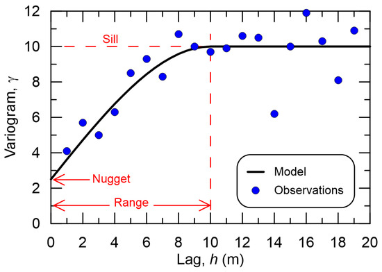
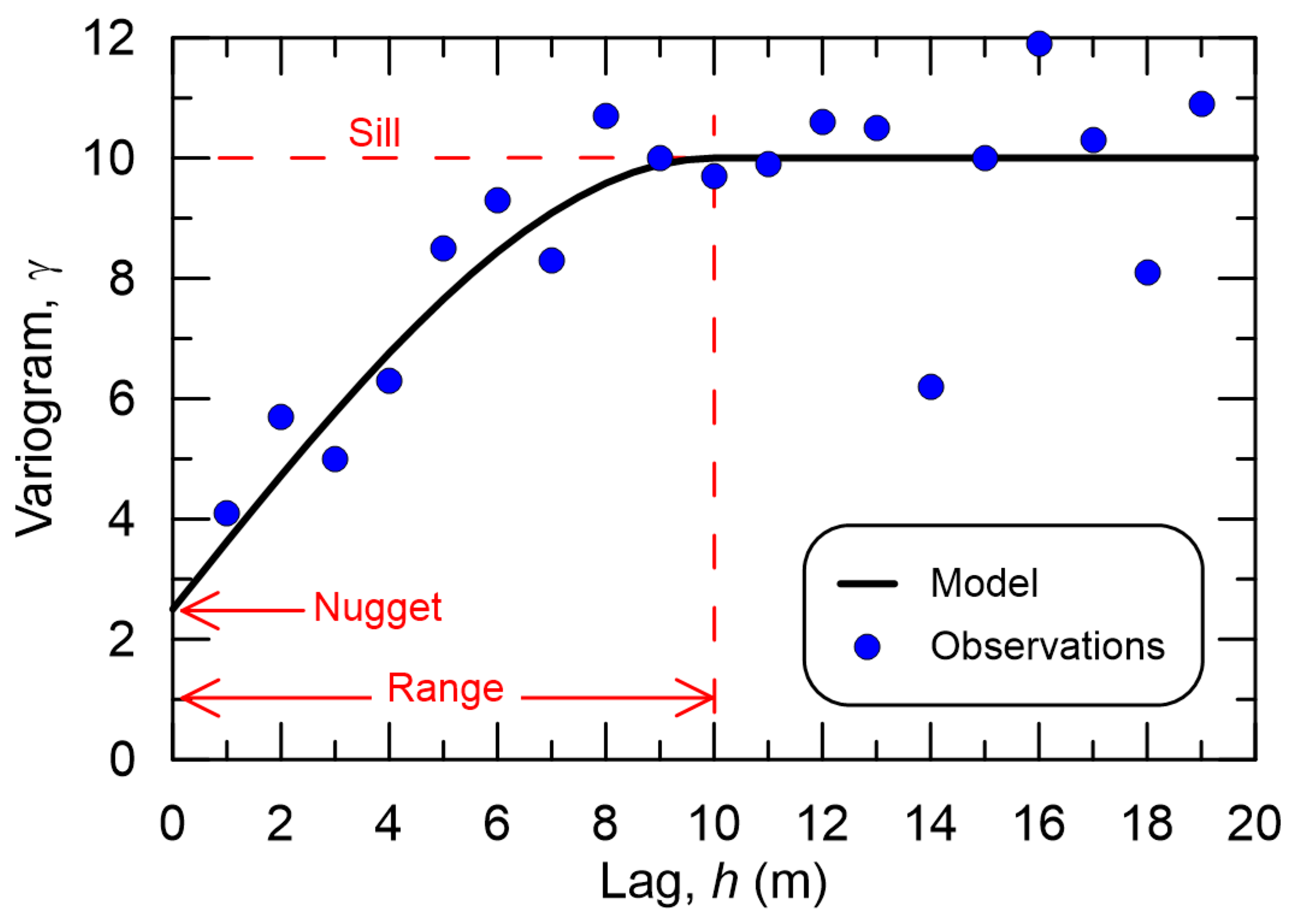
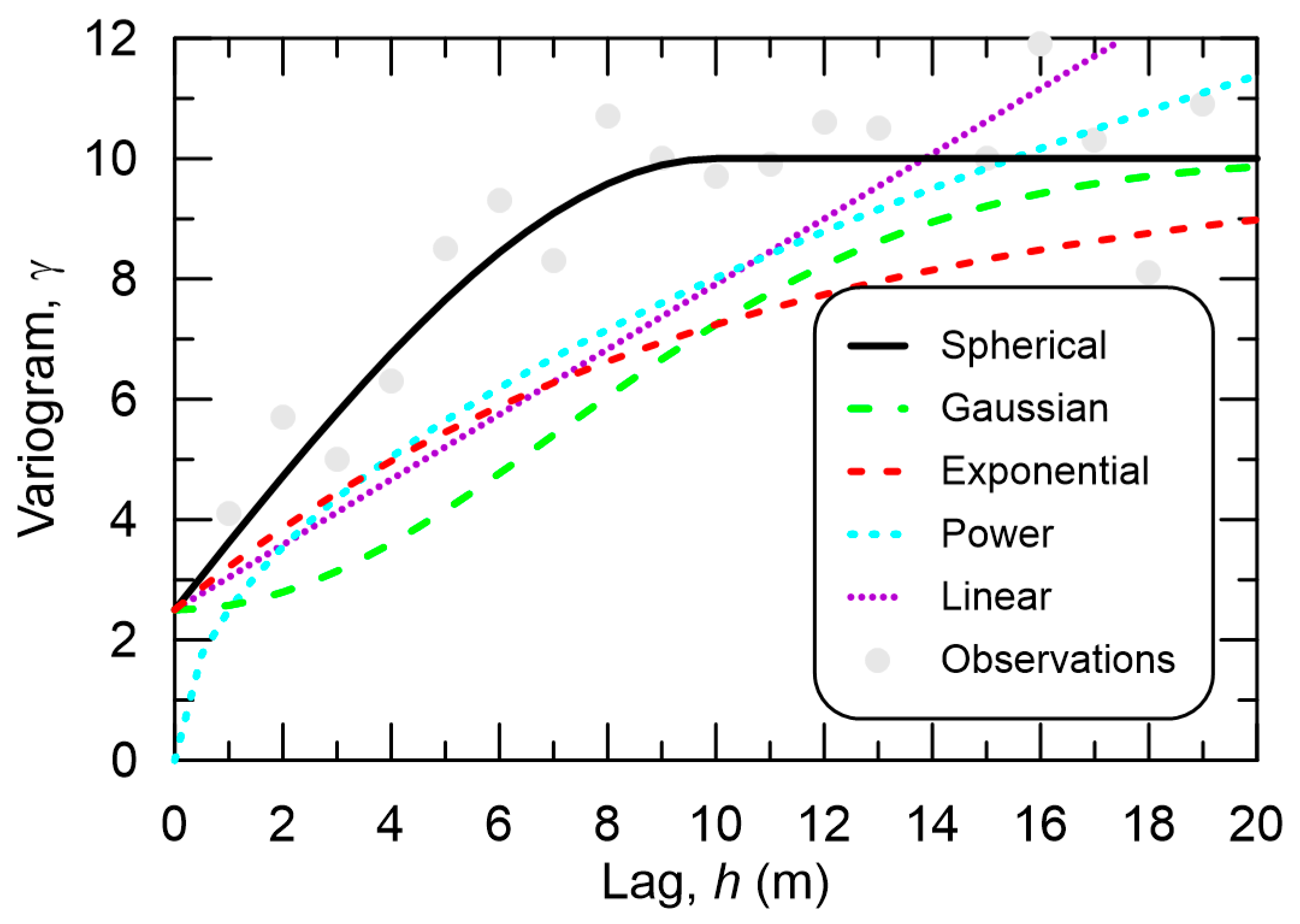
An empirical variogram is typically modeled using a specific parametric form. This is due to several assumptions and issues, one being mathematically non-negative definite for matrix inversion. This form includes parameters such as a nugget, sill, and range. A nugget is the value of the variogram at short distances, a sill is the maximum value of the variogram, while the range is the distance beyond which the data points are no longer correlated, with maximum variance. An example of these parameters is shown in Figure 2.

Figure 2. Example variogram, showing observations and a fitted variogram model. Indicators in red are shown to describe parameters. Here, nugget = 2.5, sill = 10.0, and range = 10.0.

An example variogram model is the Gaussian model. This model gently starts the initial increase in variability, which then increases rapidly after a certain distance. The Gaussian model is typically used to explain localized variability, with an example model form of:

$$\gamma \left(h\right)=Nugget+\left(Sill-Nugget\right)\left[1-\exp \left(-{\displaystyle \frac{h^2}{{Range}^2}}\right)\right]$$

(8)

Another variogram model is the Exponential model, which has the variability exponentially increase and is suitable for situations where variability continues to increase with distance when attenuation is slow. The model form is:

$$\gamma \left(h\right)=Nugget+\left(Sill-Nugget\right)\left[1-\mathit{exp}\left(-{\displaystyle \frac{h}{Range}}\right)\right]$$

(9)

The Spherical model has the variability increase linearly up to the range, after which it remains constant. The general model form is:

$$\gamma \left(h\right)=\left\{\begin{array}{c}Nugget+\left(Sill-Nugget\right)\left[{\displaystyle \frac{3h}{2Range}}-{\displaystyle \frac{1}{2}}{\left({\displaystyle \frac{h}{Range}}\right)}^3\right],ifh\le range\\ Sill,ifh>range\end{array}\right.$$

(10)

The Power-Law variogram is an interesting one in that it considers variability to continuously increase with lag. The general model for this is:

$$\gamma \left(h\right)=Coefficient\times h^{\beta }$$

(11)

where Coefficient represents some initial parameter, and $\beta$ is the Power-Law exponent, sometimes called a scaling parameter. This scaling parameter is typically $0<\beta <2$, as $\beta =0$ indicates constant variance, and $\beta =2$ describes a parabola with zero gradient at the origin, implying that the process is not random [24,25].

The simplest variogram model is the Linear model. Due to its linear form, the parameters of a sill and range are not applicable, but the nugget can be treated as an intercept or the variogram value at lag 0. An example model form is:

$$\gamma \left(h\right)=Nugget+Slope\times h$$

(12)

where Slope is the parameter representing the slope. An interesting case arises when the data fluctuates around a constant value. In this case, Slope = 0. This suggests that the variogram values are uncorrelated at the scale of the data and sample spacing. Both Power-Law and Linear variogram models are considered nonstationary models.

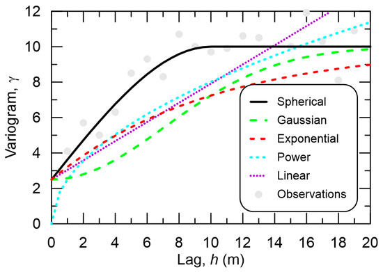
Figure 3 shows the different variogram models and their overall behavior for the same nugget = 2.5, sill = 10.0, and range = 10.0. This figure builds on Figure 2, showing example observations to give the reader a sense of how these variogram models compare when the same parameters are considered. The Linear model is regressed from the observations data, using the nugget as a fixed intercept, and only serves as a relative example. The Power model is regressed from the observations data as well but fixes the Coefficient parameter in Equation (11) to the nugget and only serves as a relative example.

Figure 3. Example variogram showing observations and Spherical, Gaussian, Exponential, and Linear variogram models. All models have a nugget = 2.5, sill = 10.0, and range = 10.0. Slope for the Linear model and exponent in Power model is regressed from the observations.

However, constructing a variogram model for use is quite tedious and perhaps subjective. Given the definition in Equation (7), a significant amount of data is required so that there are enough pairs to cover a wide range of lag. As also denoted in Equation (7), data pairs are typically grouped into lag bins, with the representative lag being the independent variable, and sometimes, there may be swaths of data missing for a bin. There is no need to have model variograms be the result of intense nonlinear regression, leaving it up to the modeler. Interestingly, the state-of-practice generally considers a good empirical variogram model as satisfying Kriging assumptions. Data that do not lend an appropriate variogram are typically considered either to be non-stationary or not spatially correlated. Thus, even if the data do not show structured spatial correlation, a modeler can still apply a relevant variogram as they deem fit. The Kriging interpolation result may not be reasonable, but it is difficult to gauge how unreasonable under the aforementioned conditions.

2.4. Ground Motion Models

From seismology and earthquake hazard studies, the vibratory ground motions that propagate away from an earthquake hypocenter will attenuate with distance and be regionally dependent [26,27,28,29,30,31,32]. It is assumed, due to these and similar factors, seismic network recorded PGA values from an earthquake may not be stationary. A typical approach in resolving such an issue is to apply Kriging to the measurement residuals from an appropriate model. In this study, two GMMs for calculating residuals are considered. One was developed from an extensive global database that closely matched measured PGA values for the 2016 Gyeongju and 2017 Pohang events [33,34]. Another GMM was based on local data and can be considered non-ergodic [35]. Non-ergodic GMMs are considered to be better than GMMs developed from global databases, as they specifically account for local behavior, typically resulting in lower uncertainties [29,30,31,32]. Kriging is used to interpolate a residual, which is then integrated back into the corresponding GMM PGA estimate at the site. For comparison and completeness, Kriging is also used to interpolate a site PGA. In this case, Kriging is used to estimate log(PGA), as ground motion intensity measures are generally log-normally distributed [34,35].

2.5. Modeling

This study would like to evaluate the outcomes of the Kriging process and its impact on estimates. In doing so, certain metrics are used to help guide the evaluation. One metric is the square of the residual sum of squares (RSS):

$$RSS=\sum _{i=1}^n{\left({measured}_i-{estimate}_i\right)}^2$$

(13)

Another similar metric is the root mean square error (RMSE):

$$RMSE=\sqrt{{\displaystyle \frac{1}{n}}RSS}$$

(14)

Another statistical metric is the Z-score:

$$Z-score={\displaystyle \frac{measured-estimate}{\sigma }}$$

(15)

which measures how many standard deviations an estimate is away from the measurement. This is used to provide guidance on how good an estimate is. In this study, a count on the number of estimates beyond the ±1.96 limit (95%) is the metric, indicative of the predictive power of the processes used. Processes that lead to many estimates beyond the limits are considered to be not as effective as those that lead to many estimates within the limits.

The aforementioned metrics are used to help evaluate an appropriate variogram model and in validating the Kriging process. For this study, 5 variogram models were presented: Linear, Power, Exponential, Gaussian, and Spherical. Regressed parameters for each variogram model are determined by minimizing RSS. The variogram model corresponding to the lowest RSS is considered the most representative of spatial behavior for the intensity measure of interest. In addition to selecting an appropriate variogram model, validating the Kriging estimate is also useful. The generally accepted approach to validation in Kriging is a process called cross-validation (CV) [36,37,38,39]. CV is generally used to find the best model amongst a field of models, and the leave-one-out cross-validation (LOOCV) technique is applied here. This technique essentially removes one data point from the data set, applies Kriging based on the subset of data, and evaluates the accuracy of the estimate. This is repeated for each point in the original data set. Typically, RMSE is the metric used in determining the cross-validation performance of the Kriging estimate.

2.6. Interpolation

For this study, Kriging interpolation is performed in two stages. The first stage is to develop a variogram model. The second stage is to perform Kriging estimates for the study sites. An assessment is made in each stage.

In the first stage, the aforementioned 5 variogram models are considered. Each empirical model is parameterized three times according to a target intensity measure estimate: log(PGA), Global GMM residual [34], and Local GMM residual [35]. Each set of parameters will have a corresponding RSS. A similar process is repeated for LOOCV, but RMSE is used to assess the variogram model and Kriging estimation process, with lower RMSE being better. To gain further insight, this study also counts the number of Z-scores in the LOOCV process beyond the 1.96 threshold (95% confidence). A higher number means the estimation ability is low, while a lower number suggests good performance. All three metrics, RSS for the variogram models, RMSE for LOOCV, and number of exceeding Z-scores, will be utilized for a holistic assessment of the best combination for the second stage Kriging interpolation.

In the second stage, the target sites considered are the Hanbit and Wolsong NPP complexes, as shown in Figure 1. For calculation purposes, the coordinates for Hanbit NPP are 126.4164° E and 35.4086° N, while the Wolsong NPP coordinates are 129.4757° E and 35.7135° N. A Kriging estimate based on findings from the first stage are compared to the site-specific GMM estimate [22]. For this study, a series of Kriging estimates are made by employing a nearest-neighbor approach; that is, an estimate is made from a subset of the measured data where the furthest measurement is removed, and Kriging is calculated from the remaining subset. This is repeated until there is only one measurement left.

All methods described herein were implemented using the Python programming language with base modules, version 3.10.9. Verification was performed using simple hand calculations and examples found in a related textbook [40]. It should be noted that there are commercial software programs that implement the different flavors of Kriging and model fitting. These commercial software programs were not used in this study.

Also note that, as shown in Figure 1, many of the stations are aligned in an “L” shape, in particular east–west, and the target sites are at the corner and edge of the “L”. This type of geometry is not conducive to anisotropic analysis, especially given the number of stations where large swaths of area will be empty.

3. Results

3.1. Variogram Models

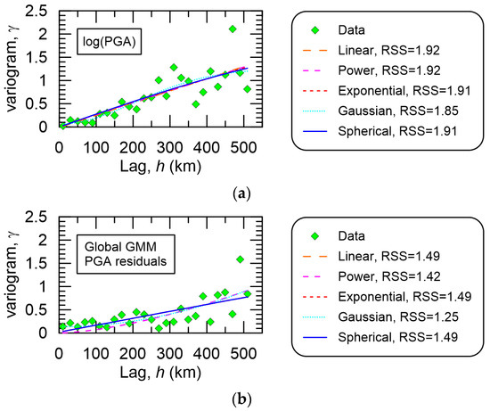
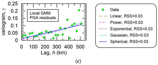
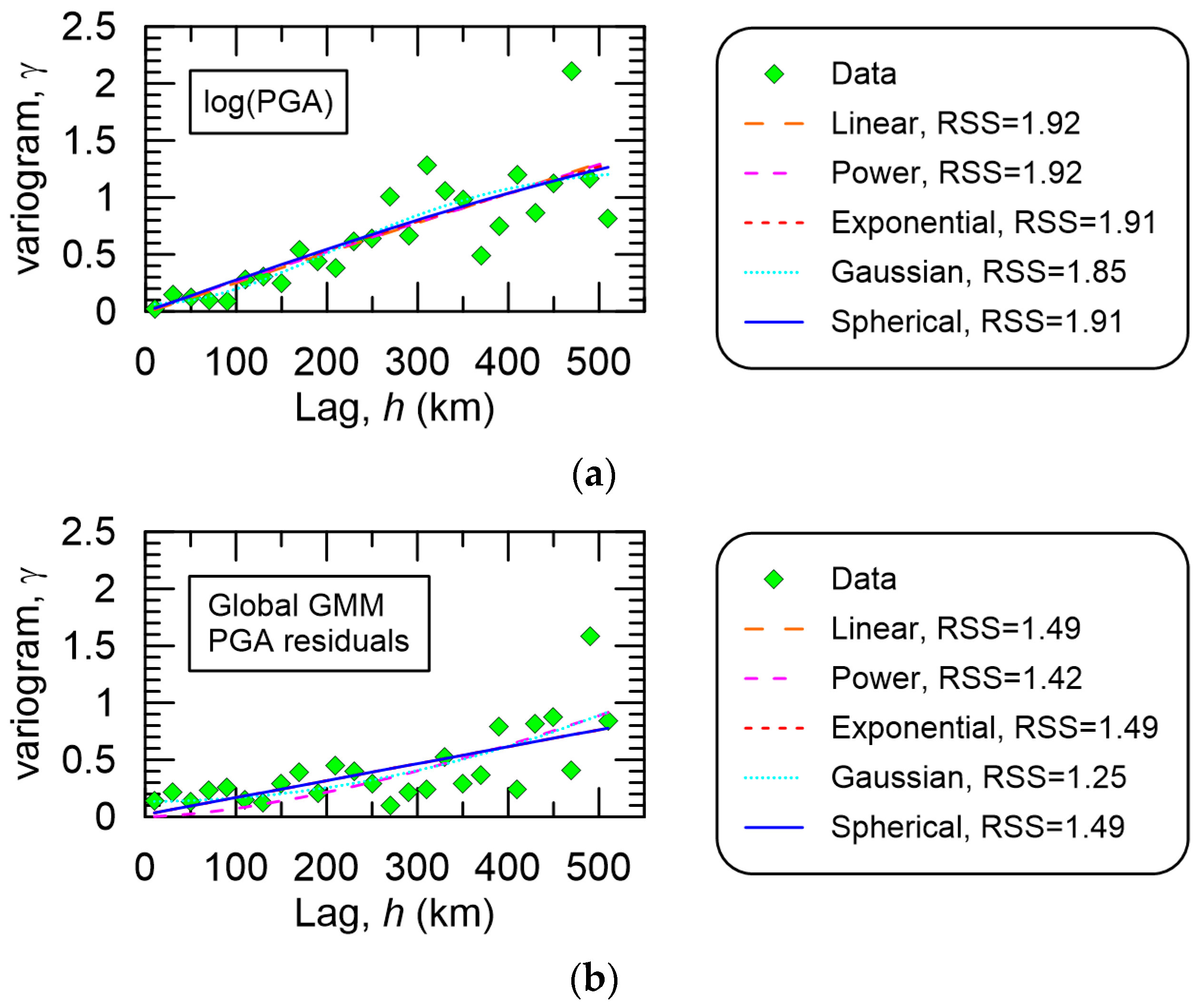
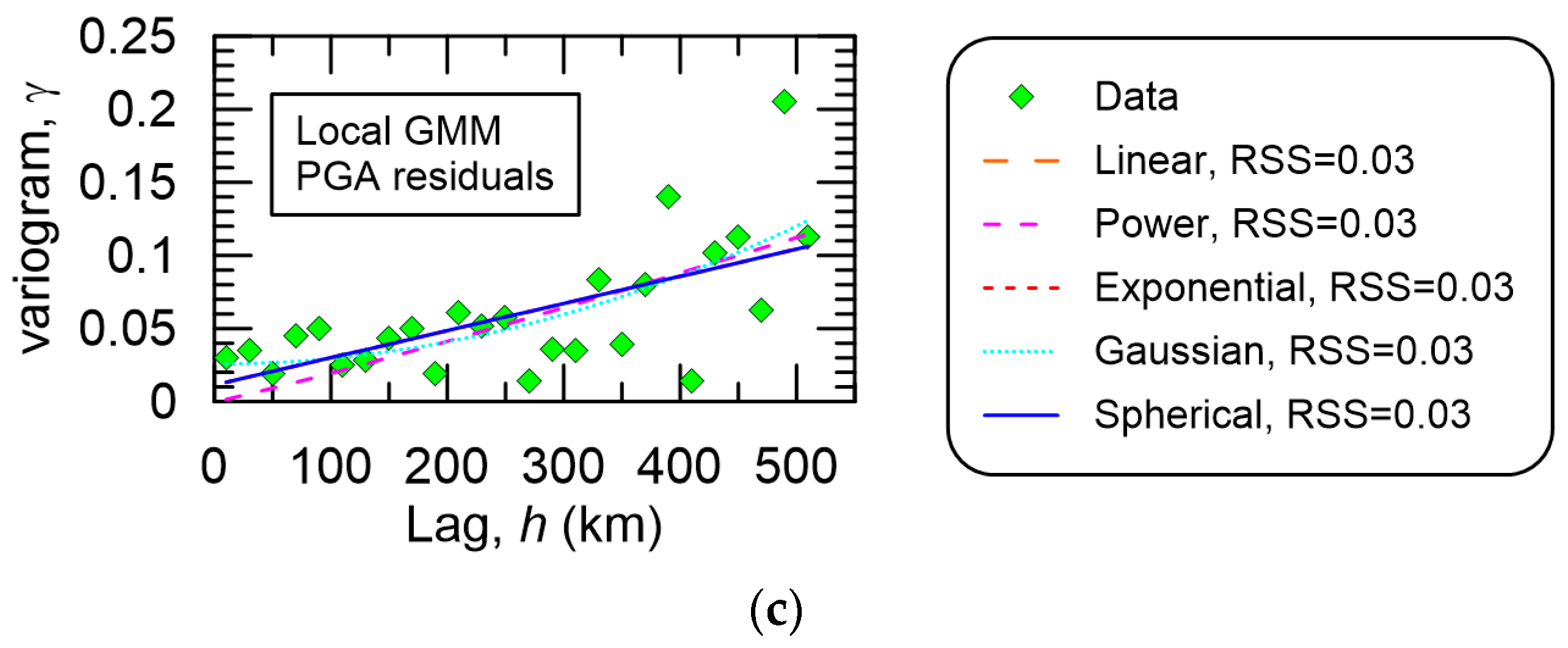
Figure 4 plots the variogram results from the KIGAM station-recorded PGAs for the 2016 Gyeongju earthquake. In the figure legend, the RSS is indicated next to the variogram model type. Figure 4a is based off of log(PGA) data, Figure 4b is based on Global GMM PGA residuals, while Figure 4c is based off of Local GMM PGA residuals. Although the figures suggest some form of spatial structure, the variability is wide at larger lags. Interestingly, the Gaussian variogram model scored the lowest RSS across the different intensity measure types, while the Linear variogram model scored the highest RSS.

Figure 4. Plots of variogram modeling for the 2016 Gyeongju earthquake. Data is shown in symbols with a bin width of 20 km. Legends list the different models considered and the corresponding regressed RSS. Variograms are based on (a) log(PGA); (b) PGA residuals when taken against the Global GMM; and (c) PGA residuals when taken against the Local GMM.

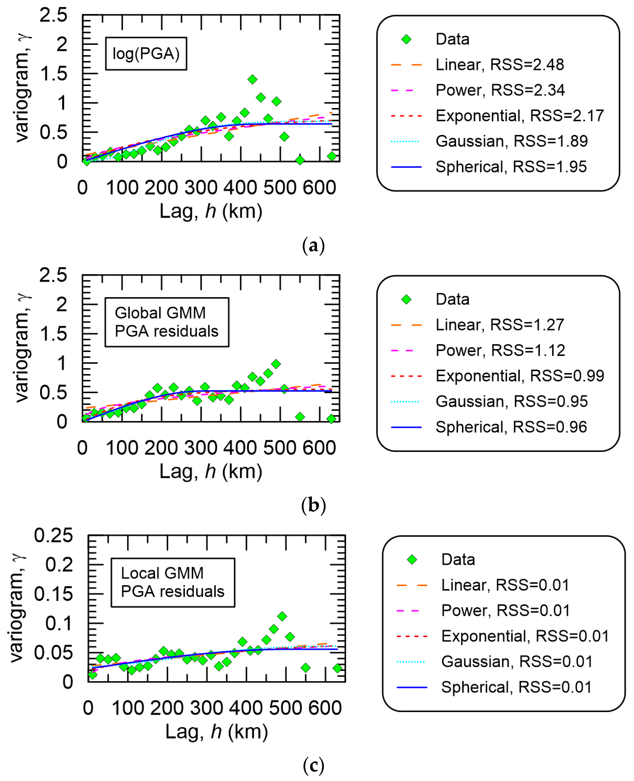
Figure 5 is the same as Figure 4 but for the 2017 Pohang earthquake. In these figures, there appears to be a drop in variance at larger lags. Similarly, the Gaussian variogram model produced the lowest RSS, while the Linear variogram model resulted in the largest RSS.

Figure 5. Plots of variogram modeling for the 2017 Pohang earthquake. Data is shown in symbols with a bin width of 20 km. Legends list the different models considered and the corresponding regressed RSS. Variograms are based on (a) log(PGA); (b) PGA residuals when taken against the Global GMM; and (c) PGA residuals when taken against the Local GMM.

Variogram parameters are summarized in Table 2. This table shows the nugget, sill, and range for Exponential, Gaussian, and Spherical variogram models for both earthquakes. The table lists the intercept and slope for the Linear variogram model as nugget and sill, respectively. The table also lists the intercept and Coefficient in the Power variogram model under the nugget and sill, respectively.

Table 2. Regressed variogram model Coefficients.

		2016 Gyeongju Earthquake [1]			2017 Pohang Earthquake [2]
Study	Variogram Model	Nugget	Sill	Range	Nugget	Sill	Range
log(PGA)	Linear 1	0.0000	0.0026		0.1073	0.0012
	Power 2	0.0029	0.9827		0.0143	0.6176
	Exponential	0.0000	7.3910	2652	0.0000	0.7772	272.5
	Gaussian	0.0627	1.2574	291.1	0.0000	0.6844	230.8
	Spherical	0.0000	1.6795	908.1	0.0000	0.6390	442.9
Global	Linear 1	0.0206	0.0015		0.2312	0.0006
GMM	Power 2	0.0000	1.5400		0.0521	0.3818
Residuals	Exponential	0.0206	5179	3,485,649	0.0000	0.5599	139.4
	Gaussian	0.1348	5582	42,997	0.0738	0.5340	155.5
	Spherical	0.0206	499.5	504,332	0.0000	0.5253	304.0
Local	Linear 1	0.0115	0.0002		0.0270	0.000006
GMM	Power 2	0.0001	1.0895		0.0079	0.3180
Residuals	Exponential	0.0115	504.3	2,715,890	0.0209	0.0714	378.3
	Gaussian	0.0258	464.4	35,083	0.0270	0.0618	306.4
	Spherical	0.0115	122.9	992,434	0.0227	0.0558	505.1

¹ For Linear variogram models, nugget represents the intercept, while sill represents the slope. ² For Power-Law variogram models, nugget represents the intercept, while sill represents the Coefficient.

3.2. Cross Validation

Results from LOOCV are shown in Table 3. The table lists results for two earthquake events. It shows the RMSE per intensity measure type and variogram model used. It also lists the number of stations with an estimate that computed a Z-score beyond the ±1.96 threshold. Interestingly, the validation results show that estimates using the Gaussian variogram model had the least favorable results regardless of the intensity measure type. The RSMEs are relatively large, primarily due to mismatches at one or two stations. Note that the Gaussian variogram model had the lowest RSS when evaluating across the different models. Overall, the table suggests Kriging estimates on Local GMM residuals for both events are the best from an RMSE perspective. Interestingly, RSMEs appear similar for both events when estimating Global or Local GMM residuals.

Table 3. LOOCV for two earthquake events. Itemized according to type of intensity measure and variogram model.

		2016 Gyeongju Earthquake [1]		2017 Pohang Earthquake [2]
Study	Variogram Model	RMSE	Z-Score (# > 95%)	RMSE	Z-Score (# > 95%)
log(PGA)	Linear	0.2451	1	0.1704	0
	Power	0.2369 a	1	0.1777	0
	Exponential	0.2438	1	0.1704	0
	Gaussian	16.1421	18	30.5337	27
	Spherical	0.2409	1	0.1644 a	1
Global	Linear	0.3951	3	0.4002	0
GMM	Power	0.4510	13	0.3661 a	1
Residuals	Exponential	0.3951	3	0.3849	2
	Gaussian	491.8429	18	32.3659	20
	Spherical	0.3951 a	3	0.3854	2
Local	Linear	0.1756 a	3	0.1692	2
GMM	Power	0.1924	12	0.1588 a	1
Residuals	Exponential	0.1756	3	0.1677	2
	Gaussian	9.4613	18	60.2304	25
	Spherical	0.1756	3	0.1686	2

^a Lowest RMSE in the group.

Another interesting observation is the overall performance for log(PGA) estimates when viewed from both an RMSE and Z-score perspective. Most notably, for the 2016 Gyeongju earthquake, LOOCV Kriging consistently underestimated station MKL below the −1.96 threshold. Surprisingly, this behavior was not reproduced in the 2017 Pohang earthquake validation process. These results suggest active site (station MKL) and source mechanisms (2016 Gyeongju). These mechanisms may have been partially captured in both GMMs used as the estimates on 2016 Gyeongju PGA residuals, as station MKL did not exceed the ±1.96 Z-score threshold on average. However, estimates for 2016 Gyeongju PGA residuals from both GMMs exceeded the ±1.96 Z-score threshold for all variogram models at stations BRS, HAK, and HKU. This switches to stations CHS and DKJ when considering the 2017 Pohang earthquake. Other than local site and source effects, there do not appear to be obvious reasons for why some stations give varying results across two earthquakes of similar magnitude and in relatively close proximity.

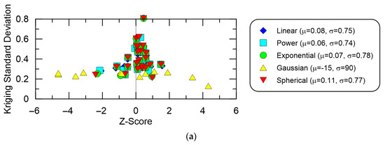
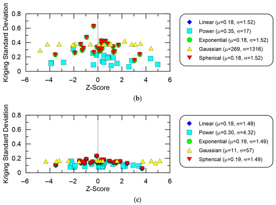
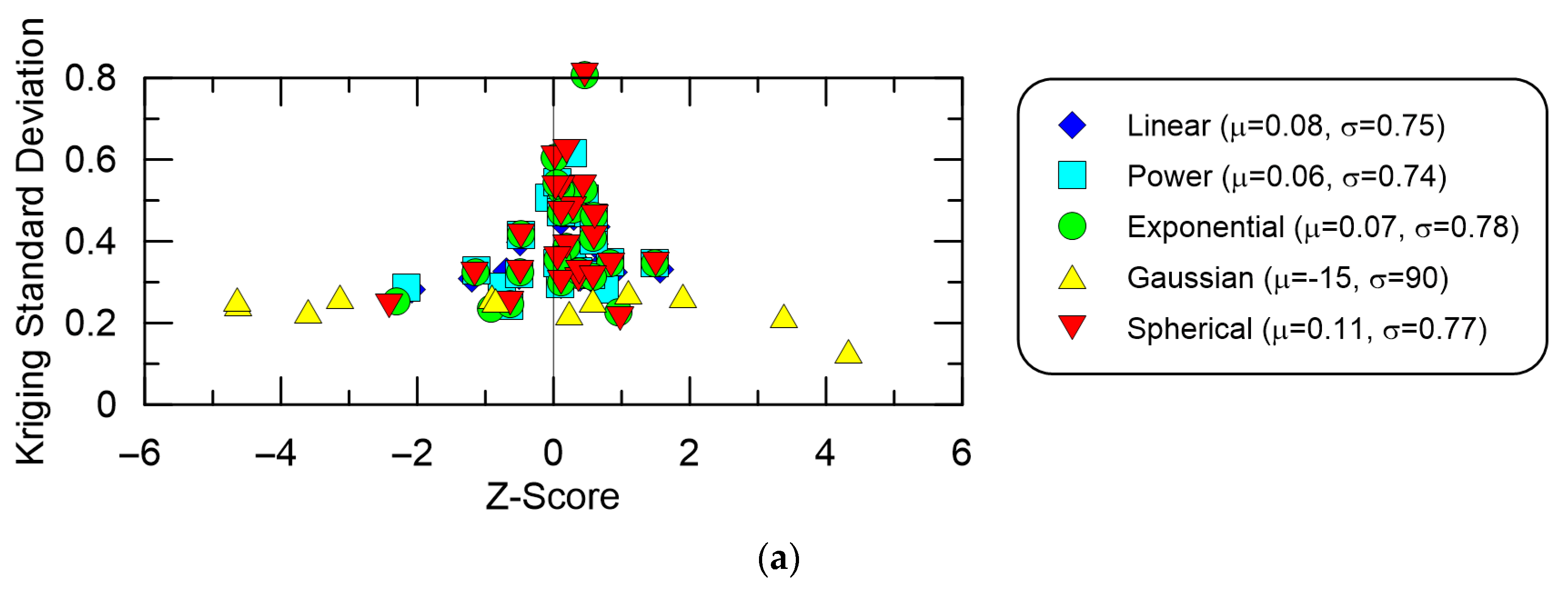
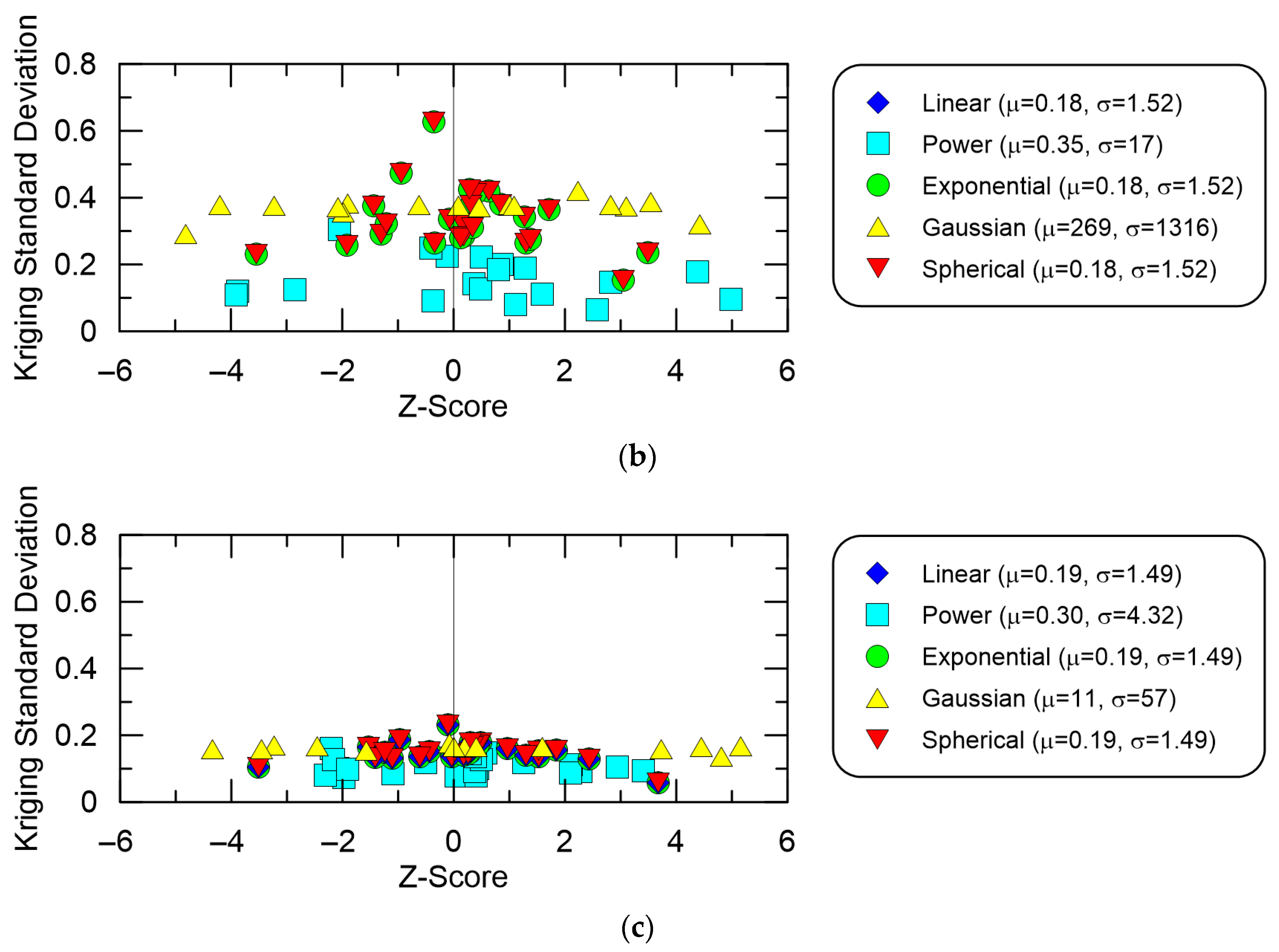
However, these Z-scores can be misinterpreted when the standard deviation is small. Figure 6 plots Z-scores against their LOOCV estimated standard deviation for the 2016 Gyeongju earthquake. Figure 6a–c show data when the intensity measure is log(PGA), the Global GMM residual, and the Local GMM residual, respectively. The legends in each graph show the mean and standard deviation of the Z-scores for the indicated variogram model. For the 2016 Gyeongju earthquake, there were 24 Z-scores used in estimating the mean and standard deviation. The means and standard deviations are relatively high, because one to three Z-scores are extreme outliers, exaggerating the results. Surprisingly, the figure suggests that Kriging standard deviations are similar for log(PGA) and Global GMM residual estimates. The low Kriging standard deviations for the Local GMM residual estimates suggest that the Z-scores may be inflated. Similar behavior was observed for the 2017 Pohang earthquake, which used 27 Z-scores.

Figure 6. Plots showing Z-score against Kriging estimated standard deviation for LOOCV for the 2016 Gyeongju earthquake. Legends list the different models considered and the associated mean and standard deviation for Z-scores. Kriging estimated standard deviation is based on (a) log(PGA); (b) PGA residuals when taken against the Global GMM; and (c) PGA residuals when taken against the Local GMM.

Based on the LOOCV process, using the Linear, Exponential, and Spherical variogram models in estimating PGA residuals from a Local GMM through Kriging works best amongst the parameters considered in this study. Considering both earthquake events, the Exponential variogram model presents a good balance of a low RMSE and fewest number of estimates exceeding a pre-determined threshold. Therefore, an Exponential variogram model is used in Kriging to estimate PGA residuals from a Local GMM.

3.3. Kriging Interpolation

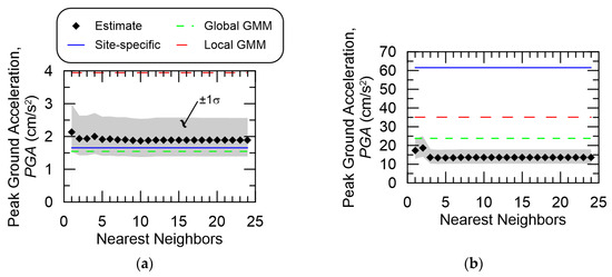
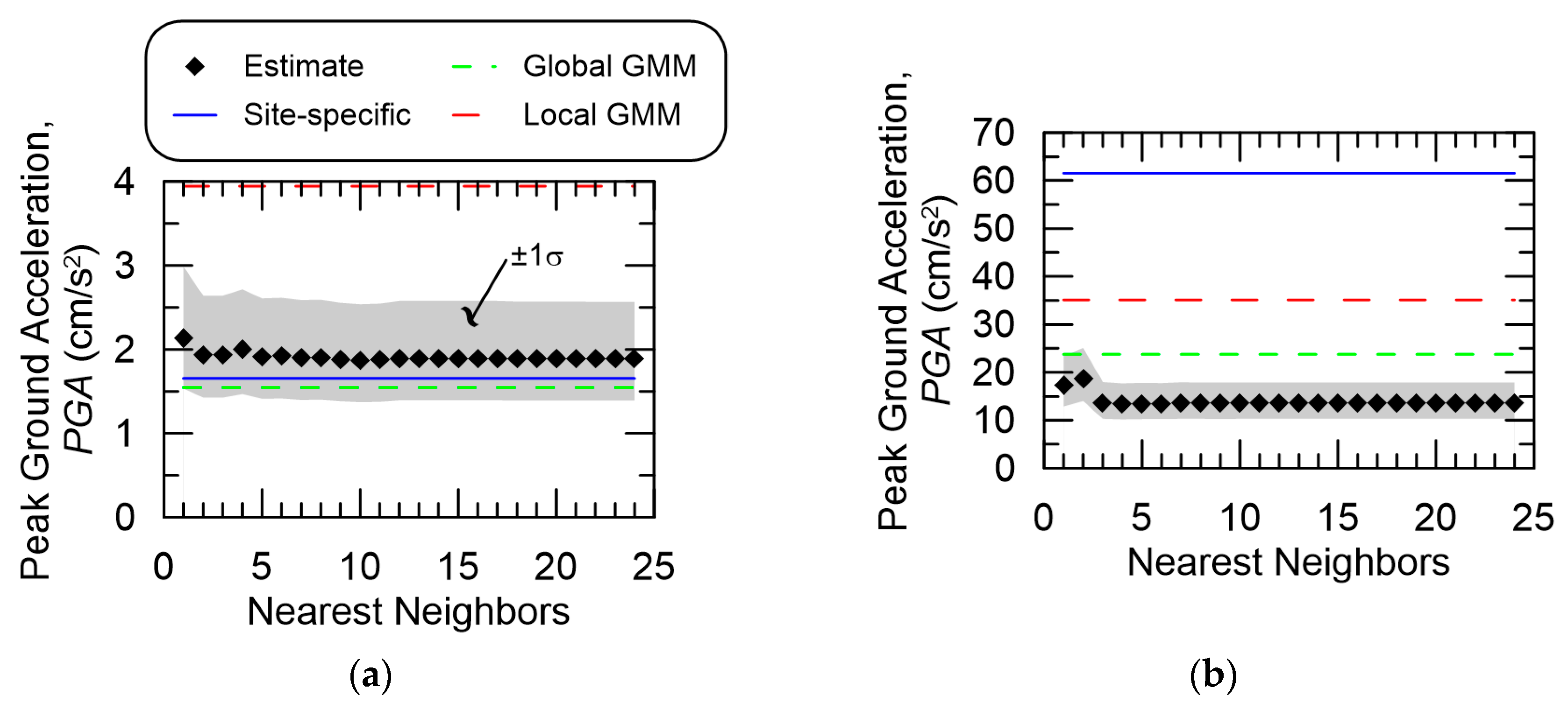
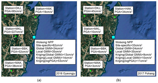
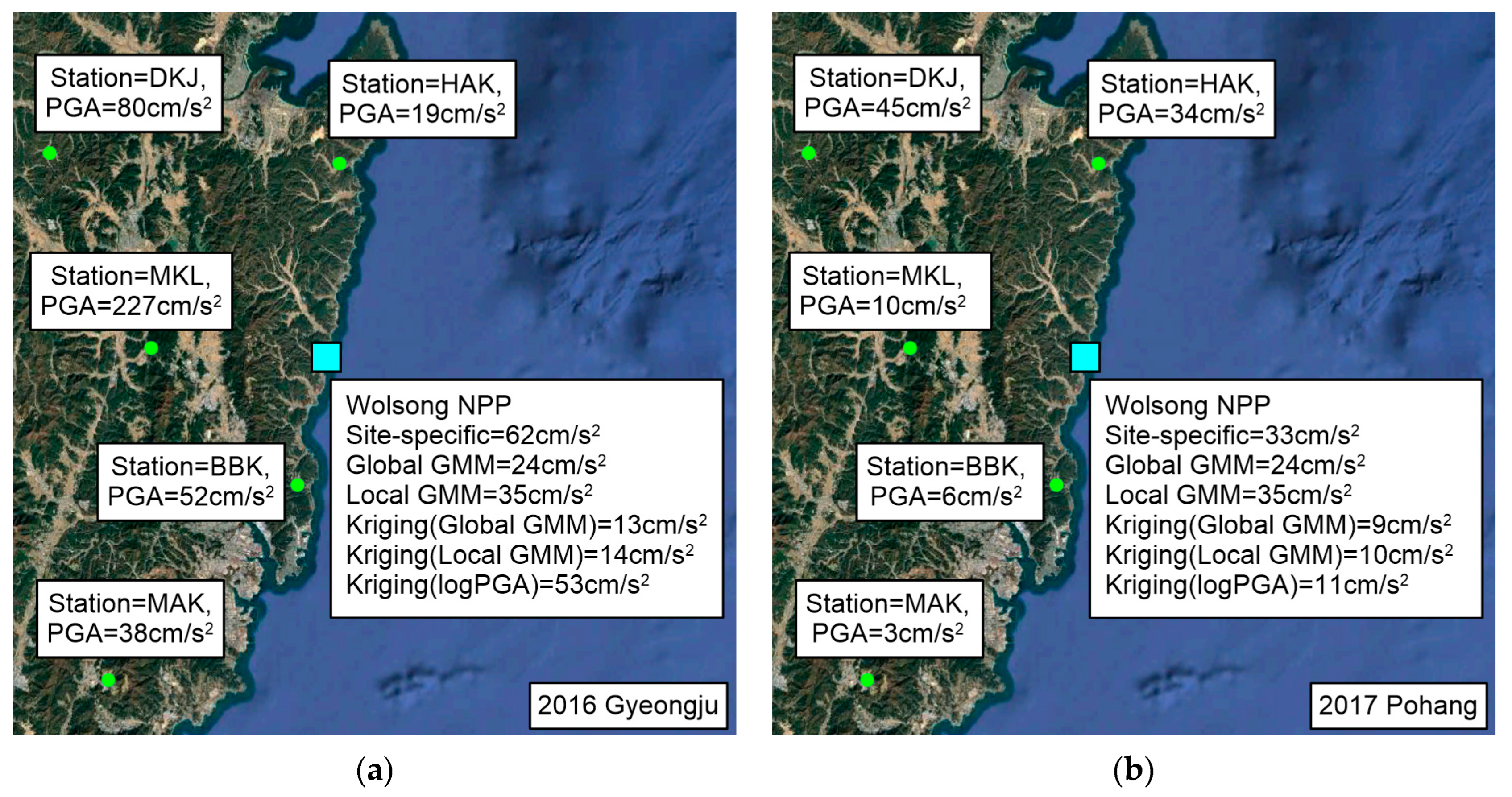
Kriging estimates are made on the two NPP locations for both earthquake events. As mentioned previously, a nearest neighbor approach is applied. Figure 7 is for the 2016 Gyeongju earthquake and plots the resultant PGA estimates against the number of closest stations to the NPP. The shaded area indicates ±1σ from the Kriging estimate. For comparison, estimates for the site-specific, Global, and Local GMMs are shown as well. Interestingly, Figure 7a shows that as the number of stations reduces to four or fewer, minor changes in the Kriging estimate and variance are apparent at Hanbit NPP. However, Figure 7b shows significant changes in the Kriging estimates and variances when there are two stations or less available for interpolation. When compared to the site-specific estimate, the Kriging estimate is within ±1σ; however, the estimate from the Global GMM is closer. Surprisingly, the estimate from the Local GMM is quite different from the other estimates. Interestingly, the Kriging, Local GMM, and Global GMM estimates are significantly less than the Wolsong NPP site-specific estimate. For the Wolsong NPP case, the three nearest recorded PGAs from the 2016 Gyeongju earthquake were 19, 36, and 227 cm/s², corresponding to stations HAK, BBK, and MKL, respectively.

Figure 7. Estimated PGA obtained by Kriging PGA residuals from a Local GMM at NPPs for the 2016 Gyeongju earthquake considering the number of closest stations. The site-specific PGA estimate is shown, along with predictions from both Global and Local GMMs. Shaded area indicates Kriging estimate ±1 standard deviation. Estimates are for the (a) Hanbit NPP and (b) Wolsong NPP.

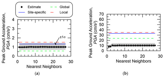
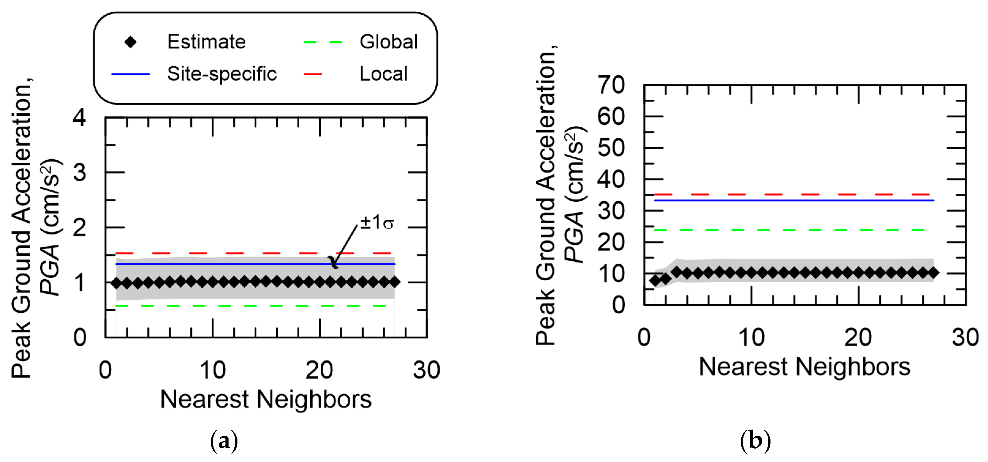
Figure 8 is similar to Figure 7 but for the 2017 Pohang event. It shows negligible difference when further stations are removed from the interpolation process. Figure 8a displays data for the Hanbit NPP, where again, the Kriging estimate is within ±1σ, but unlike the Gyeongju case, the Local GMM estimate is closer to the site-specific estimate. This is also shown in Figure 8b. Unfortunately, the Kriging estimate is the furthest from the site-specific estimate. However, in this case, the three nearest station measured PGAs were 34, 6, and 10 cm/s², corresponding to stations HAK, BBK, and MKL, respectively. These recordings are closer to the Kriging estimate than the site-specific and Local GMM estimates.

Figure 8. Estimated PGA obtained by Kriging PGA residuals from a Local GMM at NPPs for the 2017 Pohang earthquake considering the number of closest stations. The site-specific PGA estimate is shown, along with predictions from both Global and Local GMMs. Shaded area indicates Kriging estimate ±1 standard deviation. Estimates are for the (a) Hanbit NPP and (b) Wolsong NPP.

4. Discussion

Interestingly, some models ended up duplicating other models, such as the Linear, Exponential, and Spherical, where whatever benefits the structural form could offer were immensely minimized. The exaggerated parameters shown for the sill and range for the Gyeongju event shown in Table 2 result in a model similar to the Linear estimate. This was also evident in the LOOCV process. The LOOCV process also revealed a somewhat contrarian result, where the best fitted empirical variogram model performed the worst under Kriging. However, to be fair, the Gaussian model-derived RSME values were heavily skewed due to one to three exaggerated estimates across both earthquakes. This suggests that even the best fitted variogram model may not be beneficial for Kriging. Somewhat surprising, but perhaps not unexpected, was that the LOOCV process showed good performance in having Kriging estimates on log(PGA).

However, Kriging estimates at the two sites for the two events were slightly inconsistent. Estimates for Hanbit NPP tended to be better than those at Wolsong NPP. This is perhaps attributed to the order of magnitude difference in estimates. In some cases, using a GMM resulted in a better estimate. The Kriging results were relatively inconsistent as well. As an example, Figure 9 plots PGA measurements at some of the nearest stations surrounding the Wolsong NPP. The figure also shows PGA estimates from both GMMs and Kriging estimates at Wolsong NPP. An Exponential variogram model was used for consistency. Figure 9a is for the 2016 Gyeongju earthquake, while Figure 9b is for the 2017 Pohang earthquake. The measurements shown in Figure 9a appear quite diverse. Similar to Figure 8b, Global and Local GMMs were closer to the site-specific estimate than the validated Kriging estimates. Surprisingly, the Kriging PGA estimate for log(PGA) performed the best and was similar in value to station BBK. Given the model variogram and LOOCV assessment, the log(PGA) might not have been obvious. Figure 9b shows a site-specific estimate to be close to station HAK, but Kriging estimates appear to be closer to station MKL, which is very different from station BBK, as suggested by the 2016 Gyeongju earthquake. Again, these results suggest different local site and source mechanisms. These are difficult to isolate without additional information, which is not available through public channels.

Figure 9. PGA measurements at the closest stations and PGA estimates for the Wolsong NPP due to the (a) 2016 Gyeongju earthquake and (b) 2017 Pohang earthquake.

Additionally, spatial correlation did not show a strong influence on the results. This is in contrast to the aforementioned studies showing good Kriging “results” in seismically active and moderately active regions. Although a larger data set may be needed in developing an appropriate variogram model, the Kriging process suggested that a minimum of five data points is required for a consistent estimate when considering the nearest-neighbor approach. This condition was valid regardless of the variogram model used. Moreover, similar results were reached when the lag was changed to 25 and 50. This may be due to the low number of stations available for use, rendering parameters dependent on data quantity less influential. Combined with the observations from fitting an empirical variogram and LOOCV results, it would appear that studying LOOCV results is relatively more important than modeling an empirical variogram, at least in this study.

Moreover, the results can also help pinpoint specific local site and source mechanisms for non-ergodic ground shaking studies. In the LOOCV process, the results were able to identify stations that showcased measurements outside of a normal expected range. Of course, this range assumes all measurements follow the assumptions of spatial correlation, which is difficult to prove in itself. However, the principles of seismology and earthquake engineering do suggest that earthquake ground motion shaking is similar at points close to each other than at points far apart. The resulting difference stems from local site, source, and, in some cases, path effects.

5. Conclusions

Kriging estimates on different PGAs were performed at two uninstrumented sites for two moderately sized earthquakes. These sites were chosen because they have a site-specific GMM to provide a relatively good PGA estimate. Five different variogram models were considered, and LOOCV was conducted on both events with 24 and 27 PGA records, which is slightly below the literature-recommended minimum number of data points. A variety of metrics were utilized to ascertain how effective the Kriging estimates were relative to the site-specific estimates. Even with the numerous tools utilized in this study, the various metrics, and the multitude of considerations, it appears that applying Kriging for earthquake ground motion intensity measures in a small network is inconsistent.

References

- M 5.4–6 km S of Gyeongju, South Korea. Available online: https://earthquake.usgs.gov/earthquakes/eventpage/us10006p1f/executive (accessed on 21 April 2025).
- M 5.5–7 km SW of Heunghae, South Korea. Available online: https://earthquake.usgs.gov/earthquakes/eventpage/us2000bnrs/executive (accessed on 21 April 2025).
- Mercer, W.; Hall, A. The experimental error of field trials. J. Agric. Sci. 1911, 4, 107–132. [Google Scholar] [CrossRef] [Scilit]
- Krige, D.G. On the departure of ore value distributions from the lognormal model in South African gold mines. J. S. Afr. Inst. Min. Metal. 1960, 61, 231–244. [Google Scholar]
- Krige, D.G. Lognormal-de Wijsian Geostatistics for ore Evaluation, 2nd ed.; South African Institute of Mining and Metallurgy: Johannesburg, South Africa, 1981; 58p. [Google Scholar]
- Matheron, G. Principles of geostatistics. Econ. Geol. 1963, 58, 1246–1266. [Google Scholar] [CrossRef] [Scilit]
- Carr, J.R.; Glass, C.E. Use of geostatistics for accurate mapping of earthquake ground motion. Geophys. J. Int. 1989, 97, 31–40. [Google Scholar] [CrossRef] [Scilit]
- Carr, J.R.; Deng, E.D.; Glass, C.E. An application of disjunctive kriging for earthquake ground motion estimation. Math. Geol. 1986, 18, 197–213. [Google Scholar] [CrossRef] [Scilit]
- Sugai, M.; Mori, Y.; Ogawa, K. Application of kriging method into practical estimations of earthquake ground motion hazards. J. Struct. Constr. Eng. 2015, 80, 39–46. (In Japanese) [Google Scholar] [CrossRef] [Scilit]
- De Rubeis, V.; Tosi, P.; Gasparini, C.; Solipaca, A. Application of Kriging Technique to Seismic Intensity Data. Bull. Seismol. Soc. Am. 2005, 95, 540–548. [Google Scholar] [CrossRef] [Scilit]
- Linkimer, L. Application of the kriging method to draw isoseismal maps of the significant 2002–2003 costa rican earthquakes. Rev. Geol. Am. Cent. 2008, 38, 119–134. [Google Scholar] [CrossRef] [Scilit]
- Webster, R.; Oliver, M.A. How Large a Sample is Needed to Estimate the Regional Variogram Adequately? In Geostatistics Tróia ’92, 1st ed.; Soares, A., Ed.; Springer: Dordrecht, The Netherlands, 1993; Volume 5, pp. 155–166. [Google Scholar] [CrossRef] [Scilit]
- Aumond, P.; Can, A.; Mallet, V.; Coensel, B.D.; Ribeiro, C.; Botteldooren, D.; Lavandier, C. Kriging-based spatial interpolation from measurements for sound level mapping in Urban Areas. J. Acoust. Soc. Am. 2018, 143, 2847–2857. [Google Scholar] [CrossRef] [Scilit]
- ASTM D5922-25; ASTM International, Standard Guide for Analysis, Interpretation, and Modeling of Spatial Variation in Geostatistical Site Investigations. ASTM International: West Conshohocken, PA, USA, 2025.
- Thompson, E.M.; Wald, D.J. Developing Vs30 Site-Condition Maps By Combining Observations With Geologic And Topographic Constraints. In Proceedings of the 15th World Conference on Earthquake Engineering, Lisbon, Portugal, 24–28 September 2012. [Google Scholar]
- Thompson, E.M.; Wald, D.J.; Worden, C.B. A vs30 map for California with geologic and topographic constraints. Bull. Seism. Soc. Am. 2014, 104, 2313–2321. [Google Scholar] [CrossRef] [Scilit]
- Geyin, M.; Maurer, B.W. U.S. National VS30 Models and Maps Informed by Remote Sensing and Machine Learning. Seismol. Res. Lett. 2023, 94, 1467–1477. [Google Scholar] [CrossRef] [Scilit]
- Zhou, J.; Li, L.; Li, X.J.; Yu, Y.X.; Tian, Q.J. Lateral variations of shear wave velocity (vs) profile and vs30 over gentle terrain. Soil Dyn. Earthq. Eng. 2023, 175, 108265. [Google Scholar] [CrossRef] [Scilit]
- Hoang, P.H.; Phan, H.N.; Nguyen, D.T.; Paolacci, F. Kriging Metamodel-Based Seismic Fragility Analysis of Single-Bent Reinforced Concrete Highway Bridges. Buildings 2021, 11, 238. [Google Scholar] [CrossRef] [Scilit]
- Xing, L.; Gardoni, P.; Zhou, Y. Kriging metamodels for the dynamic response of high-rise buildings with outrigger systems and fragility estimates for seismic and wind loads. Resilient Cities Struct. 2022, 1, 110–122. [Google Scholar] [CrossRef] [Scilit]
- Abdelmalek-Lee, E.; Burton, H. A dual Kriging-XGBoost model for reconstructing building seismic responses using strong motion data. Bull. Earthq. Eng. 2024, 22, 3563–3589. [Google Scholar] [CrossRef] [Scilit]
- Korea Electric Power Research Institute. Technological Development for Seismic Safety Evaluation Basis of NPP Sites. Evaluation of Maximum Potential Earthquake for Nuclear Power Plant Sites; Report number: KINS/GR-335; KEPRI/TR.E08.C2006.225; Korea Electric Power Research Institute: Daejeon, Republic of Korea, 2011; 529p. [Google Scholar]
- Geo Big Data Open Platform. Available online: https://data.kigam.re.kr/ (accessed on 12 August 2024). (In Korean)
- Kitanidis, P.K. Introduction to Geostatistics: Applications to Hydrogeolog; Cambridge University Press: Cambridge, UK, 1997; pp. 61–63. [Google Scholar]
- Oliver, M.A.; Webster, R. Basic Steps in Geostatistics: The Variogram and Kriging; Springer: New York, NY, USA, 2015; 106p. [Google Scholar]
- Abrahamson, N.; Silva, W.; Kamai, R. Summary of the ASK 14 ground motion relation for active crustal regions. Earthq. Spectra 2014, 30, 1025–1055. [Google Scholar] [CrossRef] [Scilit]
- Boore, D.M.; Stewart, J.P.; Seyhan, E.; Atkinson, G.M. NGA-West2 equations for predicting PGA, PGV, and 5% damped PSA for shallow crustal earthquakes. Earthq. Spectra 2014, 30, 1057–1085. [Google Scholar] [CrossRef] [Scilit]
- Chiou, B.S.J.; Youngs, R.R. Update of the Chiou and Youngs NGA model for the average horizontal component of peak ground motion and response spectra. Earthq. Spectra 2014, 30, 1117–1153. [Google Scholar] [CrossRef] [Scilit]
- Liu, C.Y.; Macedo, J.; Kottke, A.R. Evaluating the performance of nonergodic ground motion models in the ridgecrest area. Bull. Earthq. Eng. 2023, 21, 5347–5373. [Google Scholar] [CrossRef] [Scilit]
- Macedo, J.; Liu, C.Y. A Nonergodic Ground Motion Model for Chile. Bull. Seismol. Soc. Am. 2022, 112, 2542–2561. [Google Scholar] [CrossRef] [Scilit]
- Sung, C.-H.; Miyake, H.; Abrahamson, N.; Morikawa, N. Nonergodic Ground-Motion Models for Subduction Zone and Crustal Earthquakes in Japan. Bull. Seismol. Soc. Am. 2024, 114, 1717–1738. [Google Scholar] [CrossRef] [Scilit]
- Liu, C.Y.; Macedo, J.; Abrahamson, N.; Kottke, A. A Nonergodic Ground-Motion Model for Türkiye. Bull. Seismol. Soc. Am. 2025, 116, 482–497. [Google Scholar] [CrossRef] [Scilit]
- Jung, S.-J.; Yee, E. Compatible Ground Motion Models for South Korea Using Moderate Earthquakes. Appl. Sci. 2024, 14, 1182. [Google Scholar] [CrossRef] [Scilit]
- Campbell, K.W.; Bozorgnia, Y. NGA-West2 ground motion model for the average horizontal components of PGA, PGV, and 5% damped linear acceleration response spectra. Earthq. Spectra 2014, 30, 1087–1115. [Google Scholar] [CrossRef] [Scilit]
- Emolo, A.; Sharma, N.; Festa, G.; Zollo, A.; Convertito, V.; Park, J.; Chi, H.; Lim, I. Ground-motion prediction equations for South Korea Peninsula. Bull. Seismol. Soc. Am. 2015, 105, 2625–2640. [Google Scholar] [CrossRef] [Scilit]
- Stone, M. Cross-Validatory Choice and Assessment of Statistical Predictions. J. R. Stat. Soc. Ser. B Stat. Methodol. 1974, 36, 111–133. [Google Scholar] [CrossRef] [Scilit]
- David, M. The Practice of Kriging. In Advanced Geostatistics in the Mining Industry, 1st ed.; Guarascio, M., David, M., Huijbregts, C., Eds.; Springer: Dordrecht, The Netherlands, 1976; Volume 24, pp. 31–48. [Google Scholar] [CrossRef] [Scilit]
- Delfiner, P. Linear Estimation of non Stationary Spatial Phenomena. In Advanced Geostatistics in the Mining Industry, 1st ed.; Guarascio, M., David, M., Huijbregts, C., Eds.; Springer: Dordrecht, The Netherlands, 1976; Volume 24, pp. 49–68. [Google Scholar] [CrossRef] [Scilit]
- Ploton, P.; Mortier, F.; Réjou-Méchain, M.; Baraloto, C.; Pelissier, R.; Ruas, D. Spatial validation reveals poor predictive performance of large-scale ecological mapping models. Nat. Commun. 2020, 11, 4540. [Google Scholar] [CrossRef] [Scilit]
- Burrough, P.; McDonnell, R. Principles of Geographical Information Systems; Oxford University Press: New York, NY, USA, 1998; pp. 138–142. [Google Scholar]
Disclaimer/Publisher’s Note: The statements, opinions and data contained in all publications are solely those of the individual author(s) and contributor(s) and not of MDPI and/or the editor(s). MDPI and/or the editor(s) disclaim responsibility for any injury to people or property resulting from any ideas, methods, instructions or products referred to in the content. |
© 2026 by the authors. Licensee MDPI, Basel, Switzerland. This article is an open access article distributed under the terms and conditions of the Creative Commons Attribution (CC BY) license.