Dynamic Analysis of the Maglev Vehicle–Turnout System Considering Spatial Magnetic–Rail Interaction

Abstract

The dynamic performance of medium- and low-speed maglev vehicle–track coupling systems, as well as the dynamic response of the vehicle body and suspension frame under suspension electromagnet failure, is of great significance for the safe operation of maglev tracks. Based on vehicle–track coupling dynamics theory, and considering the spatial dynamic magnetic rail relationship in combination with the suspension control system, a dynamic vehicle–track model incorporating suspension electromagnet failure is established. The effect of such failures on electromagnet suspension force and overall vehicle performance are analyzed. The results indicate that the theoretically calculated electromagnetic force differs significantly from the actual force. Under four electromagnet operating conditions, lateral displacement has the greatest influence on suspension force. By considering the magnetic saturation of ferromagnetic materials and the leakage effect of suspension gaps, a spatial dynamic magnetic orbit relationship is established. A single-pole suspension electromagnet fault has little effect on overall vehicle performance. When the suspension electromagnet on one side fails, the suspension frame tilts toward that side and is supported and operated by a sled. When three suspension points fail, the entire suspension frame loses its suspension state and operates fully under sled support. When a suspension frame electromagnet becomes stuck, severe fluctuations in suspension force and vehicle vibration acceleration occur. These fluctuations increase with vehicle operating speed, seriously endangering operational performance. The findings provide a fundamental theoretical basis for the safe operation and maintenance of medium- and low-speed maglev vehicles under fault conditions.

1. Introduction

With the continuous advancement of urbanization in China, the urban population has grown significantly. As a result, the demand for intracity transportation has in-creased substantially, placing higher and more stringent requirements on urban rail transit systems. Vibration and noise problems caused by traditional wheel–rail trains have become increasingly prominent, exerting a noticeable impact on the daily lives of residents living along rail lines. Medium- and low-speed maglev rail transit has emerged to address this demand, offering advantages such as strong climbing capability, low noise, environmental friendliness, enhanced ride comfort, and reduced dependence on terrain conditions. It therefore holds promising prospects for short-distance urban transportation.

A maglev vehicle is a large integrated system combining the vehicle system, track system, levitation control system, and electromagnetic propulsion system. Among these subsystems, the interaction between the electromagnet and the guide rail forms the foundation of dynamic studies of maglev train systems, as the magnetic–track relationship essentially determines the system’s dynamic characteristics [1]. The electromagnetic force is a three-dimensionally distributed force, and deriving its analytical expression requires complex elliptic integrations and equation solving, making it impossible to obtain a precise and simple closed-form solution [2].

Early researchers derived calculation formulas for electromagnetic force and electromagnetic torque under one-dimensional and two-dimensional magnetic–track relationships based on the principles of virtual work [3], conformal transformation [2,3,4], and the magnetic flux tube method [3,5,6,7]. Shi et al. [8] pioneered fundamental research on maglev rail relationships, deriving formulas for electromagnetic forces and moments under one-dimensional and two-dimensional rail conditions based on theories such as the virtual work method, conformal mapping, and magnetic flux tube method. By analyzing the characteristics of electromagnetic suspension forces under active control modes, they established a theoretical foundation for the linearization of maglev rail relationships and the study of dynamic interactions between maglev vehicles and track structures. Zhai Wanming and Zhao Chunfa et al. [1,9] acknowledged progress in two-dimensional and dynamic studies of maglev/track interactions but noted that the theoretical framework remains incomplete. They observed that while system stability research has expanded to the system level, it lacks integration with engineering practice, emphasizing the need for future research on three-dimensional maglev interactions, relevant experiments, and new stability analysis methods. Fan Yili [10] addressed vertical dynamics in medium-low speed maglev systems, proposing a piecewise linearized spring-damping model to simplify complex closed-loop control rail relationships. Multi-condition dynamic simulations verified that this model could replace full controller models with minimal error.

Given that maglev tracks and electromagnets interact through spatially distributed three-dimensional forces, and precise 3D electromagnetic distributions require integration within elliptical domains where analytical solutions are unattainable, He Guang [11] incorporated magnetic reluctance and saturation effects using Maxwell finite element software (Ansys Electronics 16.0) to refine electromagnetic force calculations and derived transverse electromagnetic damping forces for the first time. Wen Jiaolong and Zeng Shuo [12,13] conducted refined modeling studies on multi-degree-of-freedom and spatial maglev relationships: the former established a five-degree-of-freedom numerical model via 3D finite element analysis, while the latter developed a spatial maglev fitting model accounting for magnetic medium saturation and relative spatial poses. Liang Xin et al. [14,15] further investigated dynamic maglev relationships in normally conductive maglev trains, developing single-electromagnet dynamic suspension control models and maglev vehicle-bridge coupling dynamics models. Wang Zhiyu et al. [16] examined how maglev modeling approaches affect high-speed maglev vehicle dynamics simulation results.

To investigate electromagnetic characteristics of suspension modules, Tian and Chen et al. [17,18] analyzed key parameters and dimensions of electromagnets, while Li et al. [19] established principles for yoke thickness selection. Zhao et al. [9] demonstrated that 2D maglev relationships fail to capture 3D motion characteristics of suspension electromagnets on curved tracks. Consequently, finite element-based coil force analysis models [20,21,22], single-degree-of-freedom generalized Bouc-Wen hysteresis models [23], and spatial dynamic maglev models [24] became prevalent for 3D calculations. These approaches derived precise electromagnetic force analytical expressions incorporating full-circuit reluctance corrections and nonlinear magnetization curves of ferromagnetic materials [25].

As direct application of 3D electromagnetic forces in vehicle system dynamics simulations remains computationally challenging [26,27,28], maglev-track interaction forces require simplification [28,29,30,31]. Classical control theories like state feedback and PID are employed for suspension controller design due to their simplicity and engineering feasibility [31,32,33,34]. Han Xiaohan et al. [35] developed a two-stage series control model analyzing how control parameters and track beam characteristics affect maglev-track coupled vibrations. Sun et al. [36,37,38] addressed traditional controller limitations by establishing nonlinear maglev models integrated with intelligent control algorithms, designing RBF neural network estimators and minimal parameter learning sliding mode control strategies that significantly enhance control performance. Subsequently, this team proposed adaptive neural network controllers combining double-layer neural networks with reinforcement learning, incorporating input delay compensation and parameter optimization. They further improved disturbance rejection by using Gaussian process regression for precise parameter identification and backstepping sliding mode control. Zhou et al. [39,40] applied harmonic balance methods to reveal track flexibility-induced self-excited vibrations correlated with supply voltage, proposing voltage-regulated control with PI controllers. Chen et al. [41,42] developed suspension algorithms fusing sliding mode bifurcation control, acceleration feedback correction, and RBF adaptive compensation to suppress coupled vibrations. Su et al. [43] focused on high-performance control, implementing novel RBF neural networks (RBFNN) and adaptive sliding mode controllers for efficient maglev control. Yaseen et al. [44] proposed three nonlinear controllers—adaptive sliding mode control (AT-SMC), adaptive backstepping sliding mode control (ABS-SMC), and adaptive integral backstepping sliding mode control (AIBS-SMC)—for gap control, with AT-SMC demonstrating superior gap tracking and dynamic response. Wen et al. [45] introduced a Koopman operator-based data-driven control framework for maglev suspension systems. Building on this, Zhai Mingda et al. [46] proposed an online optimization algorithm using residual-driven Youla parameterization to enhance high-speed maglev suspension performance through dynamic compensation via matrix parameter adjustment. Focusing on key issues in maglev technology [47,48,49,50,51,52], these studies cover a wide range of aspects, from system dynamic characteristics and control methods to component strength and multi-body coupled vibrations. They encompass comparisons of different types of maglev systems as well as research on the control of specific components, providing multi-dimensional references for the theoretical refinement and practical application of maglev technology.

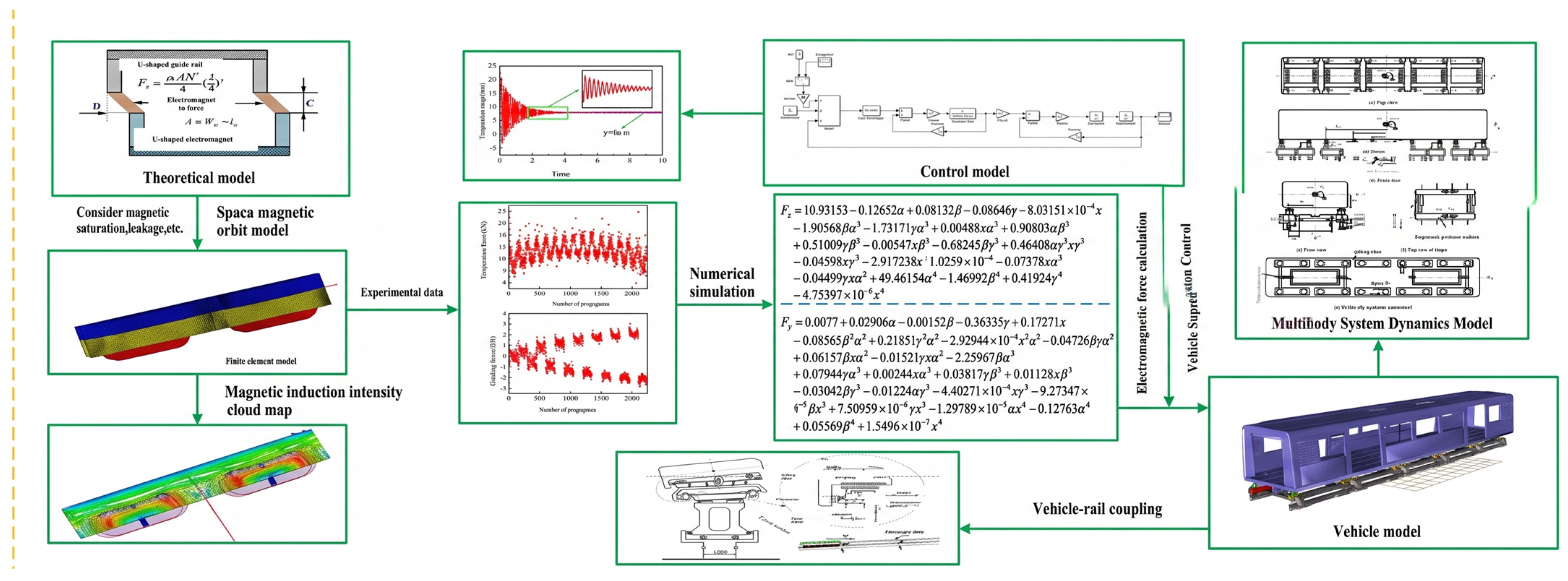
This paper constructs an analytical framework for a vehicle-turnout coupling system that integrates PID suspension control with multibody dynamics. Firstly, an engineering-feasible PID control strategy is employed in the magnetic rail modeling to achieve stable vehicle suspension control. Secondly, a high-precision dynamic model of the vehicle-turnout coupling system is established using multibody dynamics software to systematically analyze the coupled vibration characteristics between the vehicle and turnout. Considering that during normal vehicle operation, two typical failures—in-motion vehicle drop and electromagnet seizure—caused by suspension malfunctions are inevitable, this paper focuses on these two failure scenarios and conducts an in-depth investigation into the transient variations in suspension force, fluctuations in air spring forces, and the vibration response characteristics of the vehicle body. Distinguished from previous studies focusing solely on single support or suspension systems, this paper presents a coupled modeling approach that integrates PID suspension control with the track elasticity and geometric irregularities in the turnout section, thereby filling a research gap in the dynamic response analysis of low-speed maglev vehicles under suspension failure conditions in turnout areas. It reveals the cascading impact mechanisms of abrupt suspension force changes on the load distribution of air springs in adjacent suspension frames and lateral stability under two failure modes: vehicle drop and electromagnet seizure. Furthermore, this paper proposes fault severity evaluation indices based on the peak value of suspension force and the trend toward zero of the lateral force in air springs, providing direct theoretical foundations and engineering references for fault-tolerant control, speed restriction strategies in turnout sections, and redundancy design of suspension systems in low-speed maglev systems.

2. Spatial Dynamic Magnetic–Track Relationship Model

2.1. Fundamental Theory of Electromagnetic Fields

Maxwell’s equations apply to all electromagnetic phenomena. In a time-varying electromagnetic field, Maxwell’s equations can be expressed as follows:

$$\left\{\begin{array}{l}\nabla \times H=J+{\displaystyle \frac{\partial D}{\partial t}}\\ \nabla \times E=-{\displaystyle \frac{\partial B}{\partial t}}\\ \nabla \cdot D=\rho \\ \nabla \cdot B=0\end{array}\right.$$

(1)

where $H$ denotes the magnetic field intensity (A/m), $J$ denotes the current density (A/m²), $D$ denotes the electric flux density (C/m²), $E$ denotes the electric field intensity (V/m), $B$ denotes the magnetic flux density (Wb/m²), and $\rho$ denotes the charge density (C/m³).

In this study, the magnetic field of the levitation electromagnet is considered a static field. Therefore, the system of Equation (1) can be simplified as follows:

$$\left\{\begin{array}{l}\nabla \times H=J\\ \nabla \cdot B=0\end{array}\right.$$

(2)

Maxwell’s equations constitute the fundamental principles governing electromagnetic fields. In practical electromagnetic field problems, appropriate simplifications of the magnetic field region are required, corresponding boundary conditions must be imposed, and suitable transformation equations must be performed to facilitate analysis, solution, and numerical computation.

2.2. Magnetic–Track Relationship Model

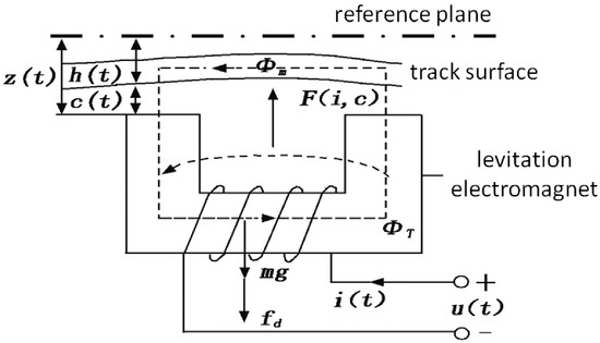
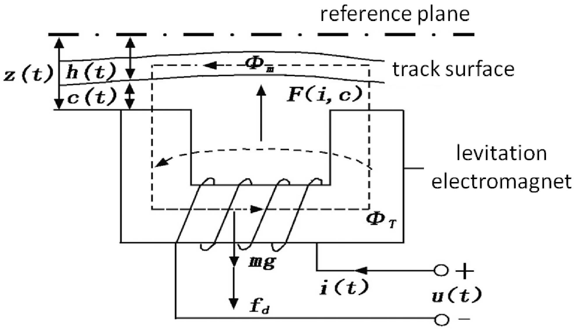
Most electromagnetic force models currently used for medium- and low-speed mag-lev vehicles are derived by transforming the system into a monopolar electromagnet mod-el using methods such as the virtual work method, conformal transformation, and the magnetic flux tube method. Therefore, in this study, an electromagnetic simulation model was developed and validated through experiments. The levitation electromagnet model is shown in Figure 1. In the figure, the position of the rail surface relative to the suspension electromagnet is represented by the equation: z(t) = h(t) + c(t), where h(t) and c(t) denote the distance between the rail surface and the reference plane, and the actual air gap, respectively. The symbols Φm and ΦT represent the air gap flux and the total flux, respectively. The variables i(t) and u(t) correspond to the current flowing through the coil and the terminal voltage, respectively. Furthermore, denoting the electromagnetic force acting on the track as F(i, c), the system dynamic equation for the suspension electromagnet in the vertical direction, subject to an external disturbance f(d), is formulated as:

$$m\ddot{z}(t)=-F\left(i,c\right)+mg+f(d)$$

Figure 1. Levitation electromagnet model.

The key parameters of the levitation electromagnet used in the magnetic–track relationship calculation are listed in Table 1.

Table 1. Key parameters of the suspended electromagnet.

Parameter	Numerical Value
Suspension electromagnet length (mm)	2650
Suspension electromagnet width (mm)	220
Magnetic pole width (mm)	28
Rated suspension gap (mm)	8
Rated coil current (A)	25
Equivalent coil winding resistance (Ω)	0.55
Number of coil winding turns (turns)	320

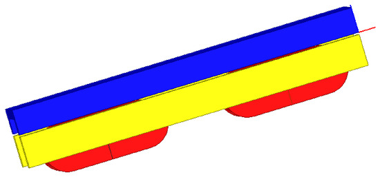
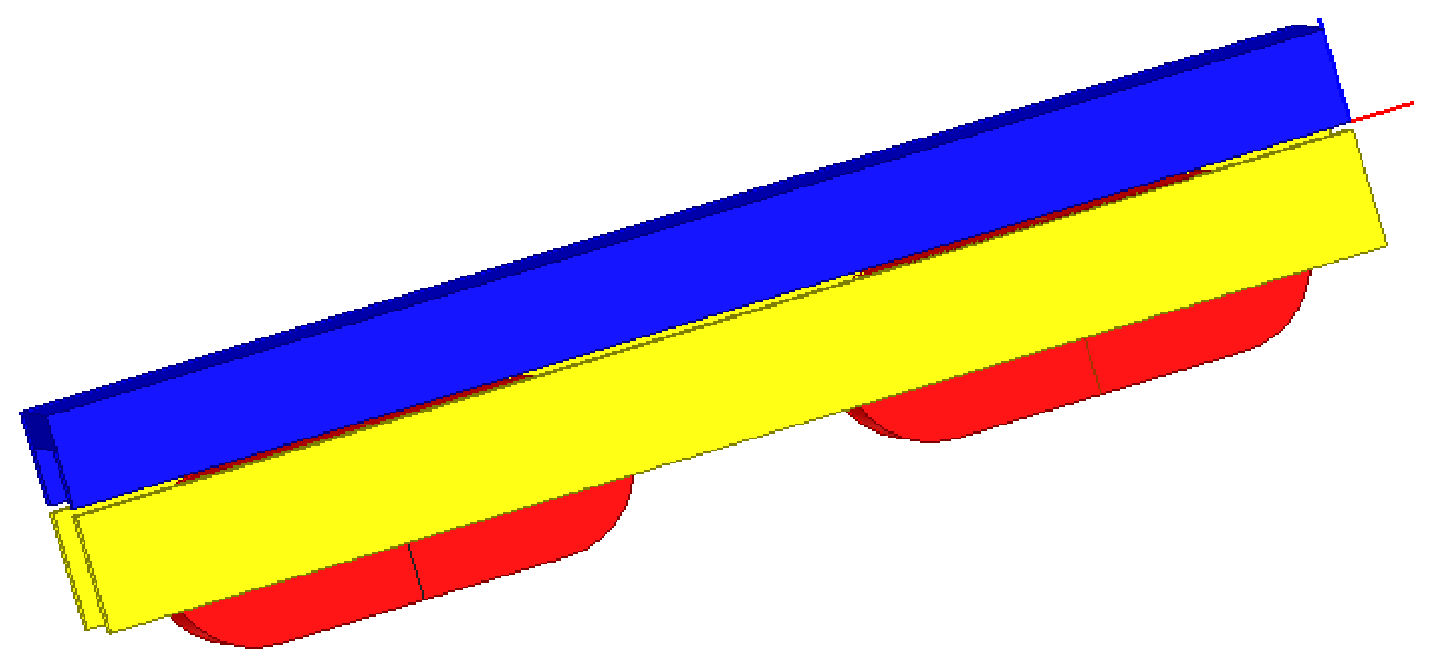
During normal operation or static levitation, the two poles of the levitation electromagnet are aligned with the corresponding poles of the track. However, during motion, track irregularities and external disturbances inevitably cause lateral displacement, yaw, roll, and pitch, leading to misalignment between the electromagnet poles and the track poles. The resulting spatial dynamic magnetic–track relationship model is illustrated in Figure 2.

Figure 2. Three-dimensional model of the electromagnet.

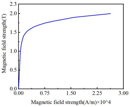
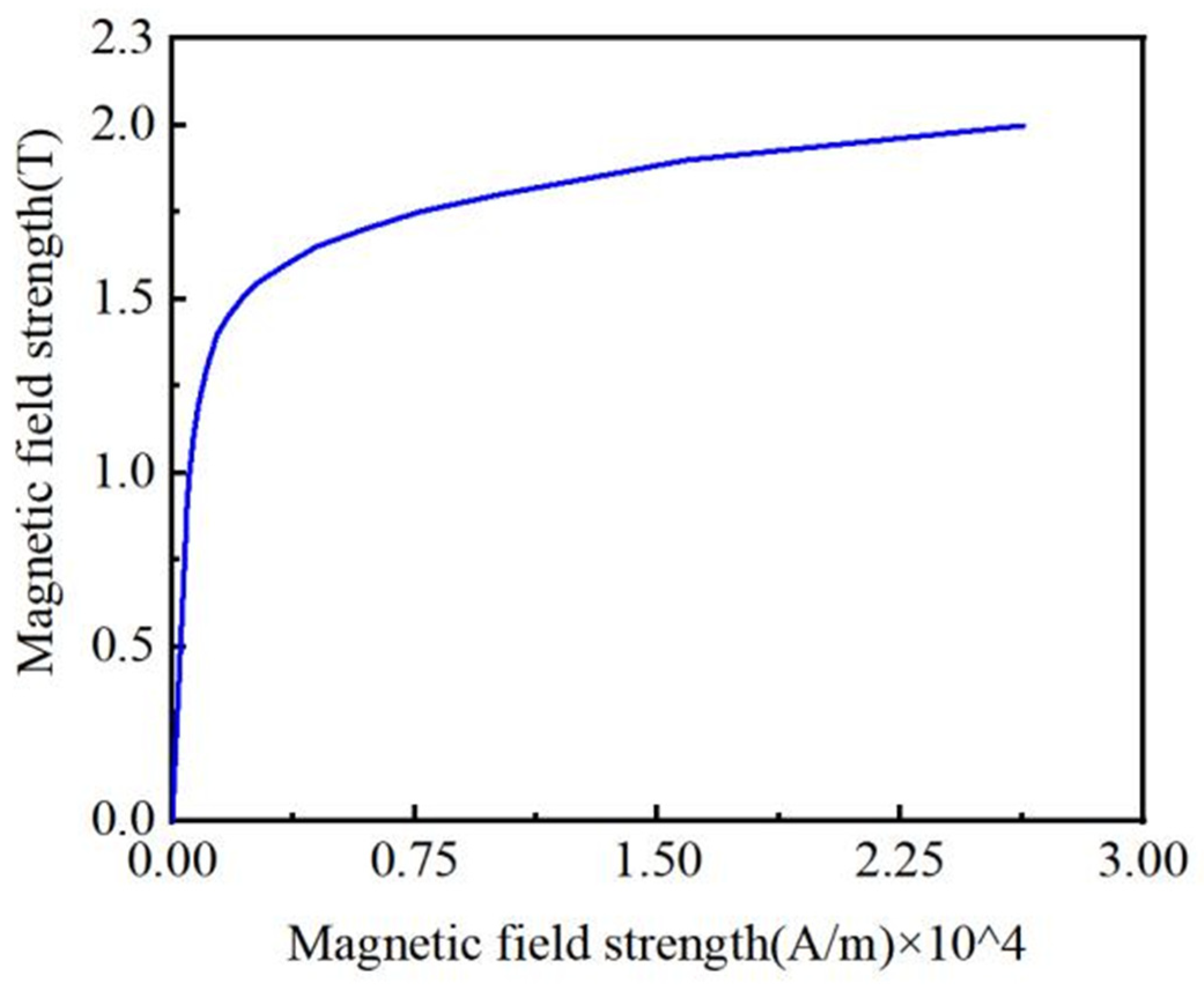
When the electromagnet undergoes lateral displacement relative to the F-type rail, the magnetic flux splits into two components: the main flux and the secondary flux. Generally, the magnetic flux entering the directly opposing pole surfaces between the levitation electromagnet and the F-rail is defined as the main flux, whereas the flux entering through non-opposing surfaces is defined as the secondary flux. This secondary flux passes through the sides of the rail and generates a lateral component of electromagnetic force, namely the guidance force. The material selected for this study is Q235, which is a ferromagnetic material widely used in engineering applications. The magnetization curve used in the calculations is shown in Figure 3.

Figure 3. Q235 magnetization curve.

2.3. Model Validation

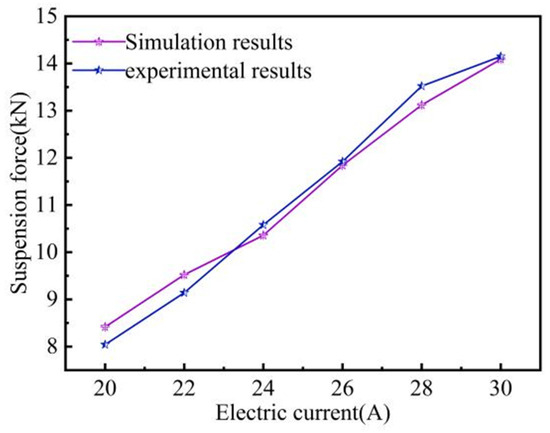
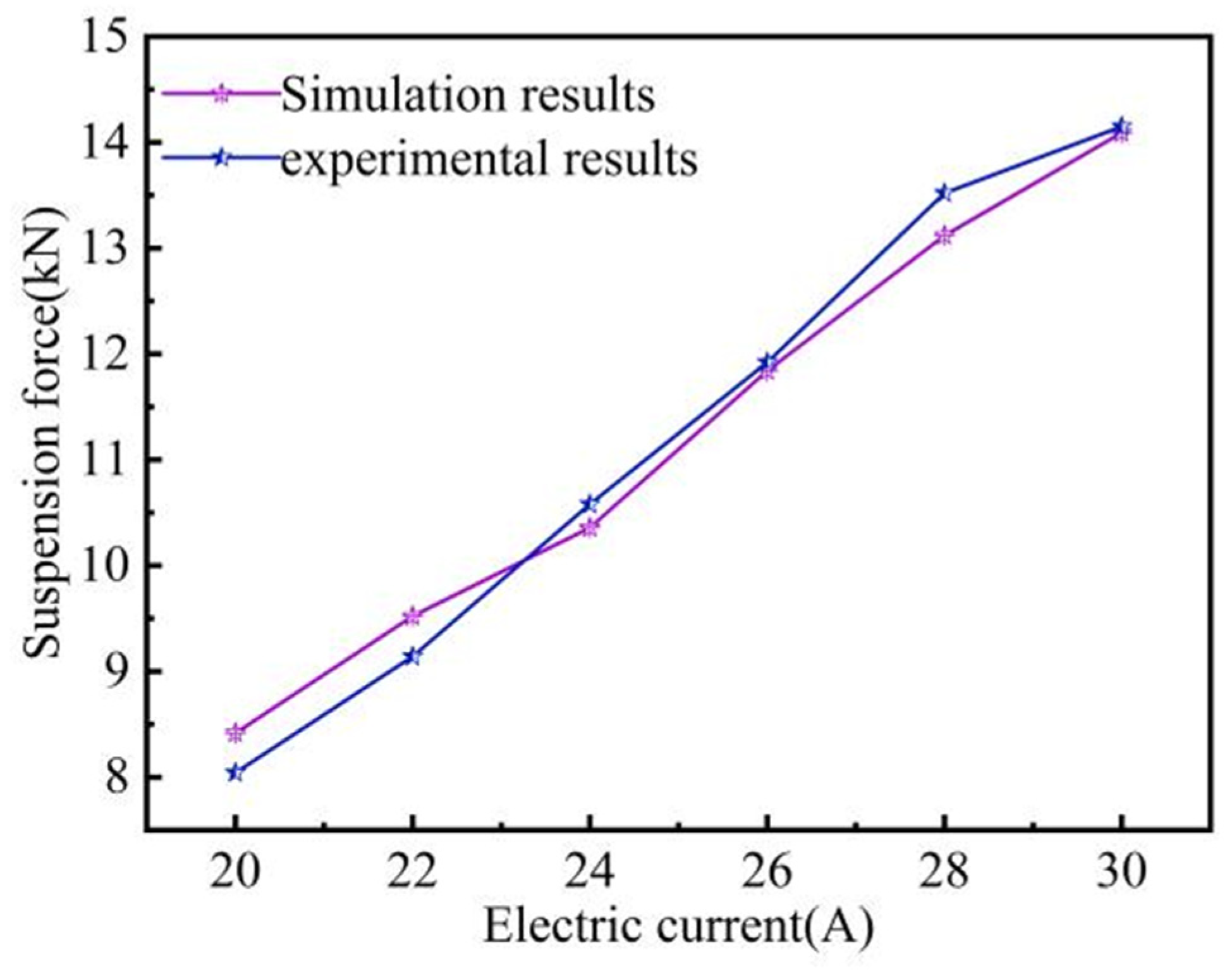
According to the working principle of the levitation electromagnet in medium- and low-speed maglev vehicles, an experimental setup for levitation force testing was constructed using a vehicle-grade electromagnet and F-rail material. The test was conducted under a fixed air gap and current. Due to experimental limitations, only the levitation force at an air gap of 8 mm was measured, as shown in Figure 4.

Figure 4. Comparison of simulation results and experimental results for levitation force.

To verify the correctness of the magnetic–track relationship model, a comparative analysis between the UM simulation results and the experimental results was conducted. As shown in Figure 4, the results obtained from the proposed magnetic–track relationship model were in close agreement with the experimental data, with only minor deviations. This demonstrates the model’s reliability and suitability for subsequent computational analyses.

2.4. Comparative Analysis of Simulation and Theoretical Models

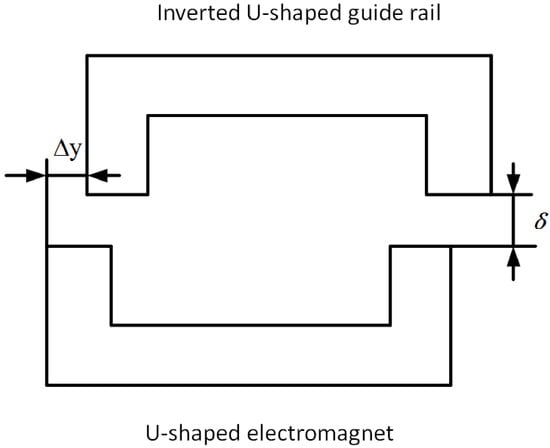
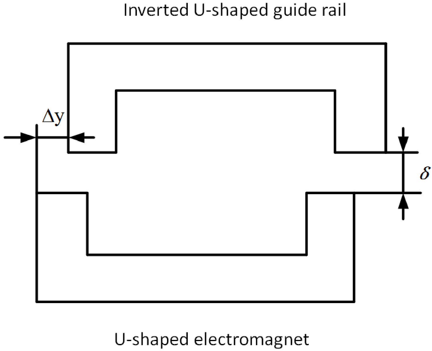
Medium- and low-speed maglev trains adopt a laterally self-stabilizing guidance method. Figure 5 shows a schematic of the magnetic–track relationship under lateral dis-placement. In the figure, the lateral displacement between the inverted U-shaped guideway and the U-shaped suspension electromagnet is denoted by Δy, and the suspension air gap is represented by δ.

Figure 5. Schematic of magnetic–track relationship under lateral displacement.

For medium- and low-speed maglev trains under lateral displacement, the levitation force and guidance force are expressed as follows:

$$F_y=F_m{\displaystyle \frac{2\delta }{\pi W_m}}\arctan ({\displaystyle \frac{\Delta y}{\delta }})$$

(3)

$$F_z=F_m\left[1+{\displaystyle \frac{2\delta }{\pi W_m}}-{\displaystyle \frac{2\Delta y}{\pi W_m}}\arctan ({\displaystyle \frac{\Delta y}{\delta }})\right]$$

(4)

where $F_m$ denotes the electromagnetic force, $W_m$ denotes the magnetic pole width, $\delta$ denotes the levitation gap, and $\Delta y$ represents the lateral displacement between the electromagnet and the guide rail.

Because the theoretical electromagnetic force formulas are derived under simplifying assumptions [37], whereas the actual electromagnetic characteristics are more complex, a combined analysis of the theoretical results and simulation results was performed.

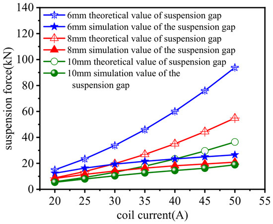
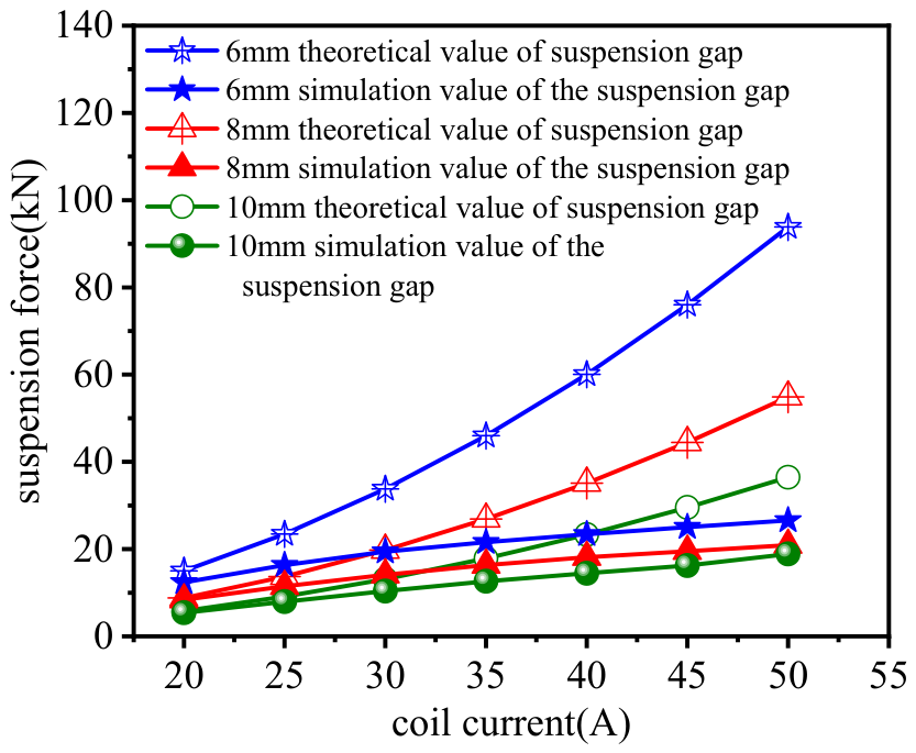
For medium- and low-speed maglev trains, the levitation gap typically varies between 6 mm and 10 mm, and the coil current fluctuates between 20 and 50 A. Three-dimensional simulations were carried out under these operating conditions, and a comparison between the simulated and theoretical levitation forces is presented in Figure 6.

Figure 6. Comparison of theoretical calculations and simulation results for levitation force.

Figure 6 shows that the theoretical solutions for suspension force are significantly higher than the 3D electromagnetic simulation values across various suspension gaps and coil currents. This discrepancy is attributed to the fact that the analytical theoretical model neglects the magnetic saturation characteristics of the ferromagnetic medium. In contrast, the numerical simulation further accounts for leakage flux losses within the spatial magnetic field; consequently, the simulated values are consistently lower than the theoretical predictions, providing a more accurate representation of the actual suspension characteristics of the electromagnet.

Furthermore, the results indicate that the suspension force increases significantly with rising coil current and decreasing suspension gap. Under the extreme operating condition of a 6mm suspension gap and a 20 A coil current, the peak 3D electromagnetic suspension force is approximately 13.7 kN, whereas it drops to approximately 7.3 kN when the gap increases to 10 mm. Caution must be exercised to prevent the risk of “drop-out” or derailment due to insufficient suspension force. Additionally, when the coil current is below 30 A and the suspension gap exceeds 8 mm, the relative deviation between the simulated and theoretical values is minimal, indicating that the analytical model maintains acceptable engineering calculation accuracy. However, as the suspension gap decreases to 6 mm, the proportion of leakage flux in the magnetic circuit rises sharply and the magnetic saturation effect intensifies. This leads to a significant increase in the relative deviation between simulation and theory, rendering the analytical model ineffective for precise calculations.

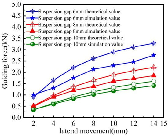
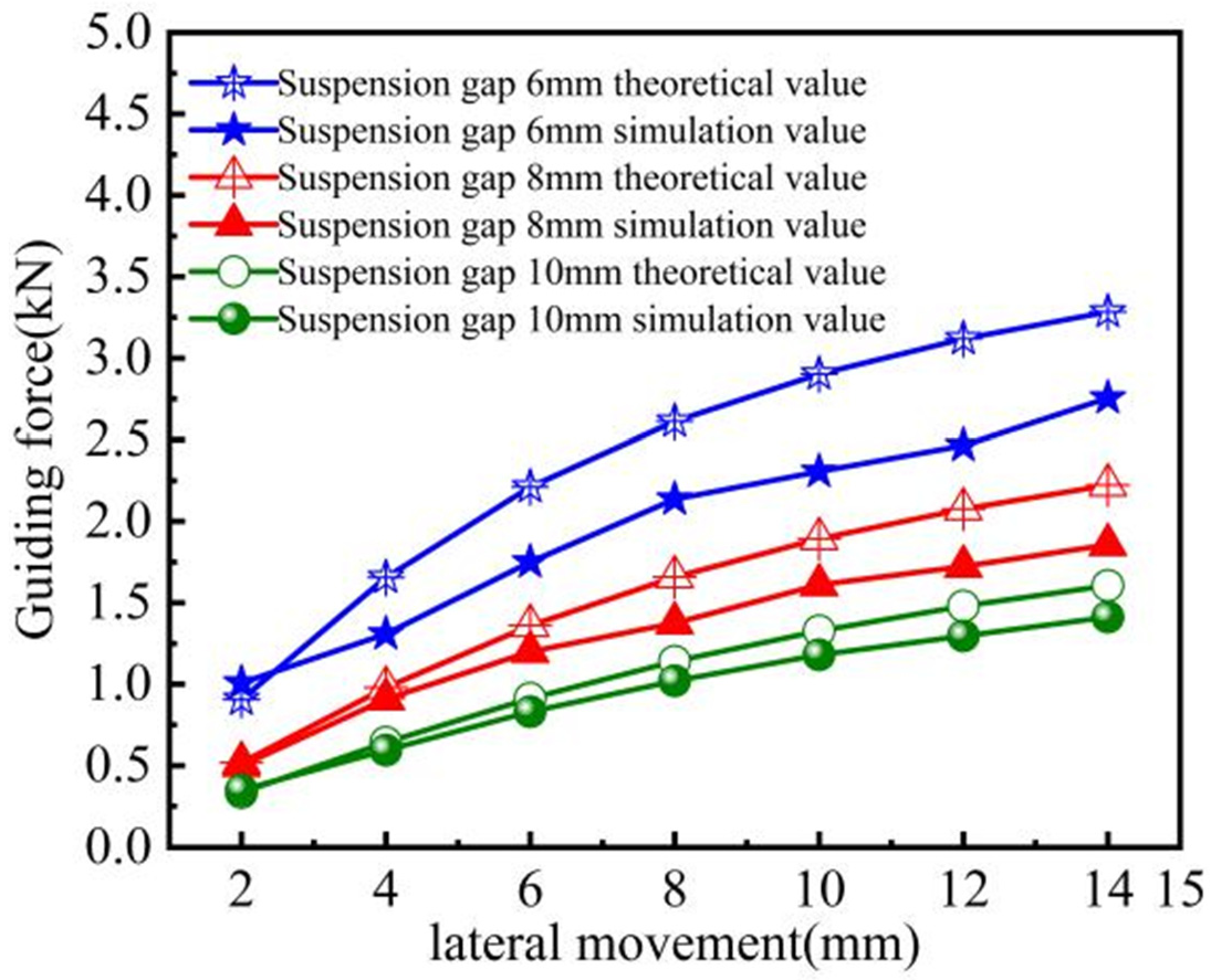
Figure 7 compares the simulated and theoretical guidance forces under lateral displacement at a rated coil current of 25 A and levitation gaps between 6 mm and 10 mm.

Figure 7. Comparison of theoretical calculations and simulation results for guidance force.

Figure 7 shows that, consistent with the suspension force results in Figure 6, theoretical guidance force values are consistently greater than 3D simulation values for all tested suspension gaps and electromagnet lateral displacements. The data indicates that guidance force rises significantly with increased lateral displacement and reduced suspension gap. At a 6 mm gap and 2 mm displacement, the simulated guidance force is approximately 1.1 kN, dropping to only 0.4 kN at a 10 mm gap, which necessitates precautions against lateral instability from force insufficiency. Moreover, the relative deviation between simulation and theory grows substantially as lateral displacement increases and the gap narrows, reaching a peak of 18.6% at a 10 mm gap and 14 mm displacement.

In summary, because the theoretical electromagnetic force is derived from simplified assumptions, notable discrepancies exist between theoretical results and simulation or experimental data. Therefore, electromagnetic simulations and experiments are necessary to recalibrate and refine the computational model so that it more accurately reflects real operating conditions.

3. Spatial Magnetic–Track Relationship Surrogate Model

The magnitude of the electromagnetic force generated by the levitation electromagnet depends not only on the levitation gap but also on four additional degrees of freedom: lateral displacement, yaw, roll, and pitch. In principle, all five degrees of freedom (including vertical motion) should be considered when calculating the electromagnetic force. However, because the subsequent vehicle model incorporates a levitation control module that maintains stable levitation through active control, the six-degree-of-freedom spatial dynamic magnetic–track model developed in this paper considers only four degrees of freedom—lateral displacement, yaw, roll, and pitch. Under the condition that the levitation module and the track do not collide, four motion parameters are defined, and their variation ranges are given in Table 2.

Table 2. Range of Variation of Motion Parameters for the Levitation Module.

Parameter	Range
Horizontal movement distance/mm	−14~14
Head shaking angle/°	−0.65~0.65
Side rolling angle/°	−0.55~0.55
Pitching angle/°	−0.46~0.46

3.1. Electromagnetic Force Simulation Under Four Operating Conditions

During maglev train operation, lateral displacement is unavoidable, resulting in relative lateral movement between the levitation electromagnet and the track. When the levitation gap remains constant, an increase in lateral displacement leads to a reduction in levitation force. At the same time, a guidance force arises that pulls the electromagnet back toward its central position. During operation, the lateral displacement between the electromagnet and the track is constrained, with a maximum allowable offset of 14 mm.

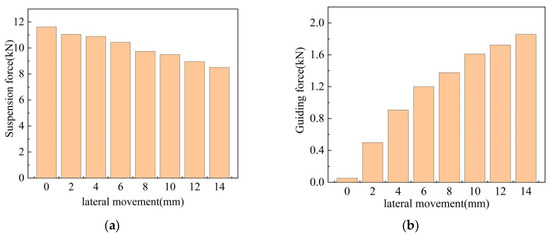
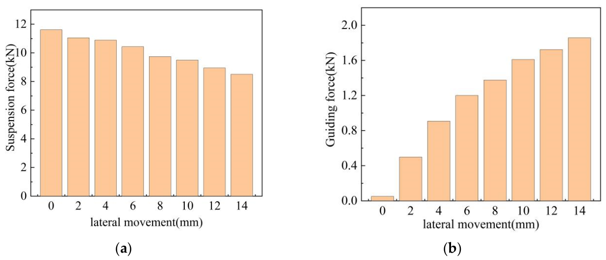
Figure 8 shows the effect of lateral displacement on electromagnetic force under an 8 mm levitation gap and a coil current of 25 A.

Figure 8. Effect of lateral displacement on electromagnetic force: (a) effect on levitation force; (b) effect on guidance force.

As shown in the results of Figure 8, with the incremental increase in the lateral offset of the electromagnet, the levitation force exhibits a continuous decline. This implies that under large-lateral-displacement operating conditions, the system is required to compensate for its load-bearing capacity by either augmenting the excitation current or reducing the levitation gap. However, such measures will inevitably intensify the control burden and elevate the risk of “sucking death” (a situation where the electromagnet and the guideway adhere tightly due to excessive magnetic attraction). Therefore, it is advisable to restrict the rated operating lateral displacement within 8 mm to reserve a sufficient safety margin.

Although the guidance force demonstrates an increasing trend with the lateral displacement and showcases a self-centering characteristic, its growth rate gradually decelerates. This indicates that in large-lateral-displacement regions (for instance, when the lateral displacement exceeds 10 mm), the guidance stiffness undergoes a significant reduction, leading to a weakened ability to resist lateral disturbances. Hence, it is recommended to set the alarm threshold at 10 mm and enhance the gain in the active guidance control or introduce lateral compensation mechanisms.

In contrast, the lateral displacement has a relatively minor impact on the traction force, which suggests that the levitation and traction systems possess excellent decoupling characteristics. Consequently, traction control can be implemented largely independently of the lateral displacement conditions, without the need for additional feed-forward corrections. This not only simplifies the design of the drive but also ensures the smooth and stable operation of the maglev system.

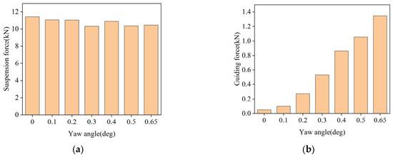
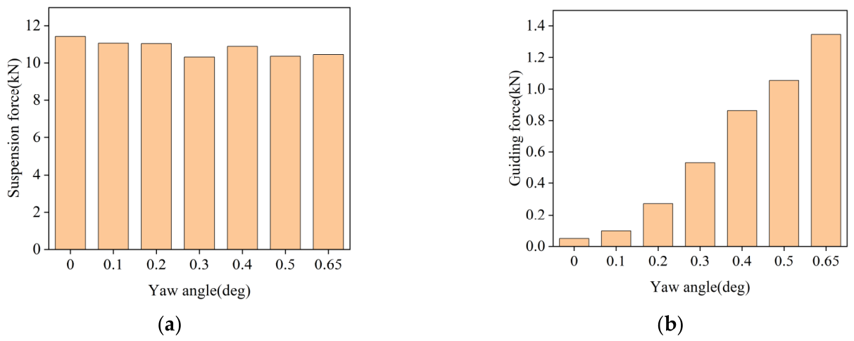
Figure 9 shows the effect of electromagnet yaw on electromagnetic forces under the same conditions (8 mm levitation gap and 25 A current).

Figure 9. Effect of yaw on electromagnetic force: (a) effect on levitation; (b) effect on guidance force.

As shown in Figure 9, when yaw motion occurs, the variation in levitation force remains within 1 kN. Meanwhile, the guidance force increases with the yaw angle, and this increase becomes more pronounced at yaw angles greater than approximately 0.1°.

During train operation, roll and pitch motions are also inevitable. However, compared with lateral displacement and yaw, these motions do not cause significant lateral misalignment between the electromagnet and the F-rail. Consequently, no guidance force is generated, or any variation is negligible and can be ignored.

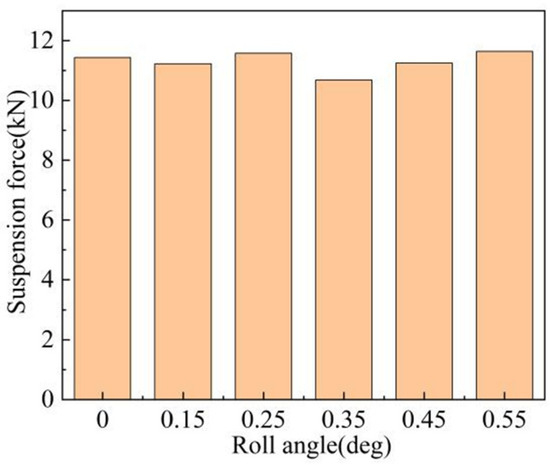
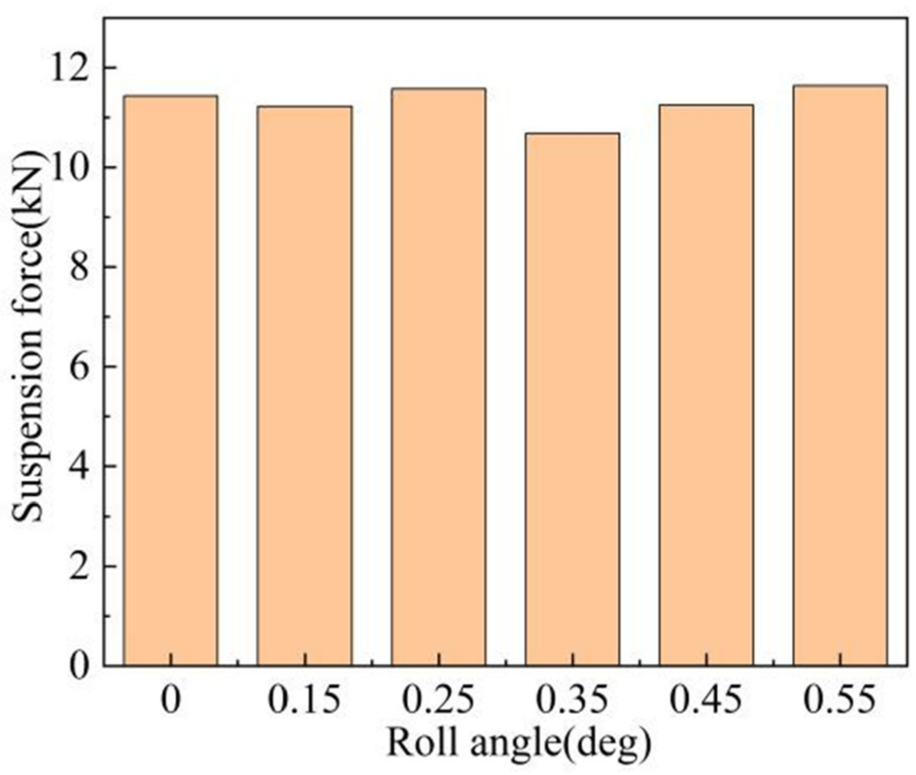
Figure 10 shows the effect of electromagnet roll on levitation force under an 8 mm levitation gap and a 25 A current.

Figure 10. Effect of roll on electromagnetic force.

As shown in Figure 10, as the roll angle increases, the levitation force exhibits only minor variations and remains relatively stable within a narrow range.

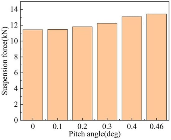
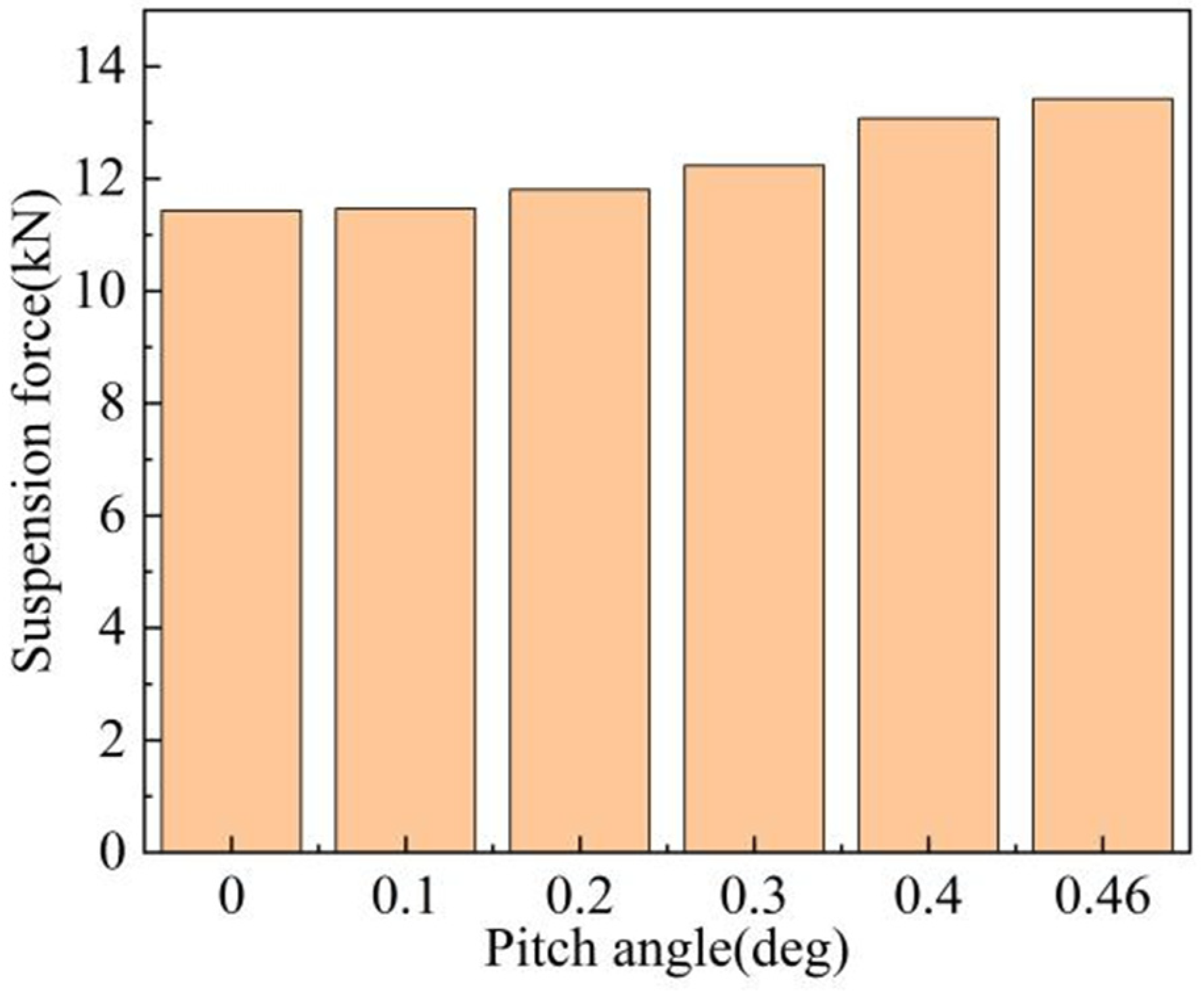
Figure 11 shows the effect of electromagnet pitch on the levitation force under an 8 mm levitation gap and a 25 A current.

Figure 11. Effect of pitch on electromagnetic force.

As shown in Figure 11, the levitation force increases significantly with increasing pitch angle and reaches a maximum of 13.42 kN at a pitch angle of 0.46°. This occurs because a larger pitch angle causes a differential change in the front and rear levitation gaps, bringing the electromagnet surfaces closer to the track and thereby significantly increasing the levitation force.

3.2. Fitting of Spatial Electromagnetic Levitation and Guidance Forces

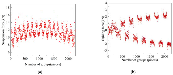
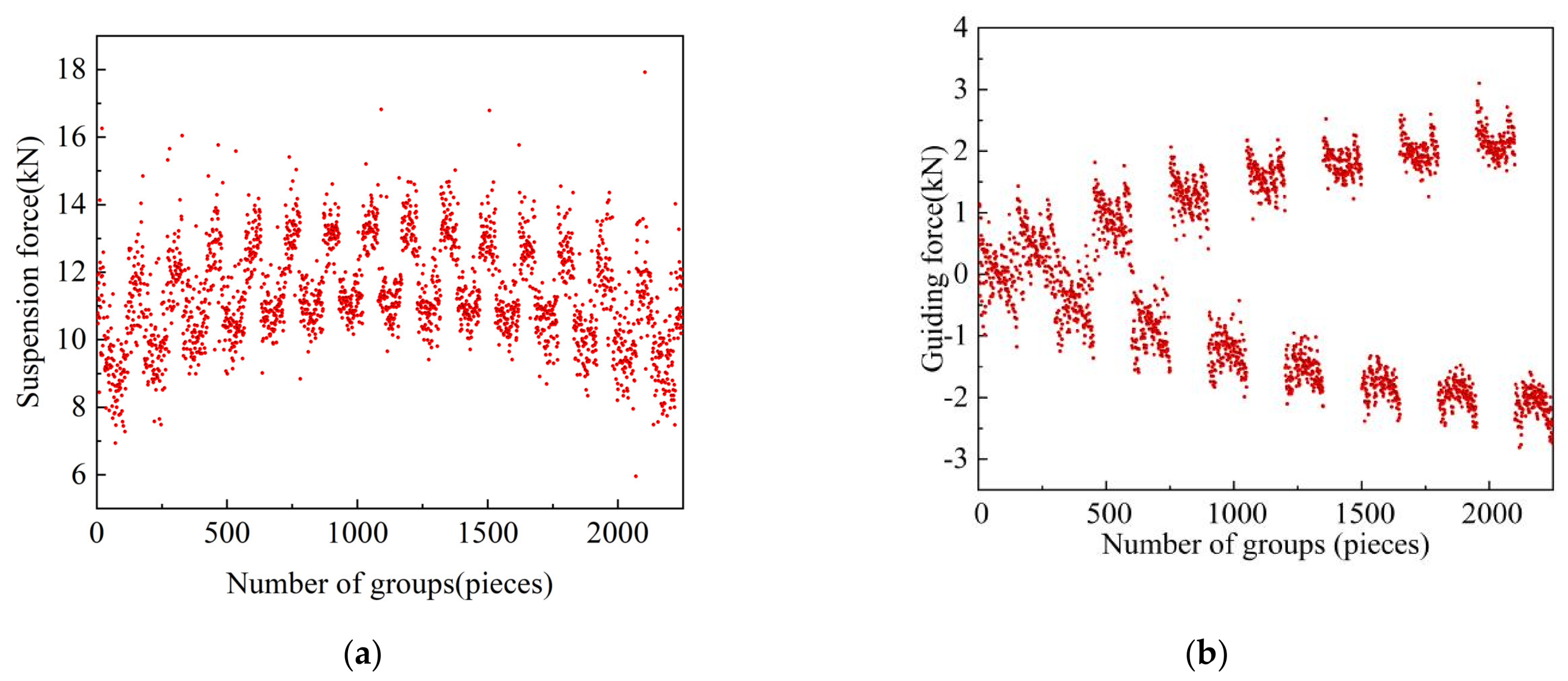
Based on the established six-degree-of-freedom spatial dynamic magnetic–track relationship model and by comprehensively considering four degrees of freedom—lateral displacement, yaw, roll, and pitch—multiple sets of simulation data were obtained using electromagnetic simulation software. The resulting data scatter plots are shown in Figure 12.

Figure 12. Scatter plot of simulation data: (a) levitation force; (b) guidance force.

Through simulation analysis, a refined dynamic magnetic–track relationship model was established by accounting for magnetic saturation effects, and a polynomial calculation model consistent with actual operating conditions was fitted as a surrogate. Terms of degree 3 or higher that consist of products of two or more variables (e.g., x³, α²β, γx², β³γ …) exhibit near-linear relationships with one another, resulting in a high degree of correlation among high-order cross terms. Consequently, the fitted complex polynomial function does not exhibit a simple convergent trend, as illustrated in Figure 12b.

Because analytical formulas for electromagnetic force are typically derived using simplified assumptions, this study constructed a spatial dynamic magnetic–track model and performed simulation analyses. Based on the computed data from multiple simulation cases, a final polynomial-based surrogate model was developed.

For the levitation force, the polynomial fitting model is expressed as

$$\begin{array}{l}{F}_z=10.93153-0.12652\mathsf{\alpha }+0.08132\mathsf{\beta }-0.08646\mathsf{\gamma }-8.03151\times {10}^{-4}x\\ -1.90568\mathsf{\beta }{\mathsf{\alpha }}^3-1.73171\mathsf{\gamma }{\mathsf{\alpha }}^3+0.00488x{\mathsf{\alpha }}^3+0.90803\mathsf{\alpha }{\mathsf{\beta }}^3+0.51009\mathsf{\gamma }{\mathsf{\beta }}^3\\ -0.00547x{\mathsf{\beta }}^3-0.68245\mathsf{\beta }{\mathsf{\gamma }}^3+0.46408\mathsf{\alpha }{\mathsf{\gamma }}^3-0.04598x{\mathsf{\gamma }}^3-2.917238\\ \times {10}^{-5}\mathsf{\beta }{x}^3-1.0259\times {10}^{-4}\mathsf{\gamma }{x}^3-9.28364\times {10}^{-5}\mathsf{\alpha }{x}^3+0.52675{\mathsf{\alpha }}^2{\mathsf{\beta }}^2\\ +3.50337{\mathsf{\alpha }}^2{\mathsf{\gamma }}^2-0.00578{\mathsf{\alpha }}^2{x}^2-0.97186\mathsf{\beta }\mathsf{\gamma }{\mathsf{\alpha }}^2+0.07301\mathsf{\beta }x{\mathsf{\alpha }}^2\\ -0.04499\mathsf{\gamma }x{\mathsf{\alpha }}^2+49.46154{\mathsf{\alpha }}^4-1.46992{\mathsf{\beta }}^4+0.41924{\mathsf{\gamma }}^4\\ -4.75397\times {10}^{-5}{x}^4\end{array}$$

(5)

For the guidance force, the polynomial fitting model is expressed as

$$\begin{array}{l}{F}_y=0.0077+0.02906\mathsf{\alpha }-0.00152\mathsf{\beta }-0.36335\mathsf{\gamma }+0.17271x-0.08565{\mathsf{\beta }}^2{\mathsf{\alpha }}^2\\ +0.21851{\mathsf{\gamma }}^2{\mathsf{\alpha }}^2-2.92944\times {10}^{-4}{x}^2{\mathsf{\alpha }}^2-0.04726\mathsf{\beta }\mathsf{\gamma }{\mathsf{\alpha }}^2+0.06157\mathsf{\beta }x{\mathsf{\alpha }}^2\\ -0.01521\mathsf{\gamma }x{\mathsf{\alpha }}^2-2.25967\mathsf{\beta }{\mathsf{\alpha }}^3+0.07944\mathsf{\gamma }{\mathsf{\alpha }}^3+0.00244x{\mathsf{\alpha }}^3-1.50138\mathsf{\alpha }{\mathsf{\beta }}^3\\ +0.03817\mathsf{\gamma }{\mathsf{\beta }}^3+0.01128x{\mathsf{\beta }}^3-0.03042\mathsf{\beta }{\mathsf{\gamma }}^3-0.01224\mathsf{\alpha }{\mathsf{\gamma }}^3-4.40271\times {10}^{-4}x{\mathsf{\gamma }}^3\\ -9.27347\times {10}^{-5}\mathsf{\beta }{x}^3+7.50959\times {10}^{-6}\mathsf{\gamma }{x}^3-1.29789\times {10}^{-5}\mathsf{\alpha }{x}^4-0.12763{\mathsf{\alpha }}^4\\ +0.05569{\mathsf{\beta }}^4-0.09258{\mathsf{\gamma }}^4+1.5496\times {10}^{-7}{x}^4\end{array}$$

(6)

where $x$ represents the lateral displacement, $\alpha$ denotes the pitch angle, $\beta$ denotes the roll angle, and $\gamma$ denotes the yaw angle.

The primary challenge in deriving theoretical expressions for the magnetic–track relationship lies in the complexity of elliptical domain integrals, which makes it difficult to obtain simplified closed-form solutions. Therefore, a refined dynamic magnetic–track relationship model was established by conducting detailed simulation analyses and accounting for magnetic saturation effects. The resulting polynomial fitting model served as a practical surrogate for the theoretical formula and provided a realistic computational basis for electromagnetic force calculations in subsequent levitation control simulations.

4. Levitation Control System

4.1. Mathematical Model

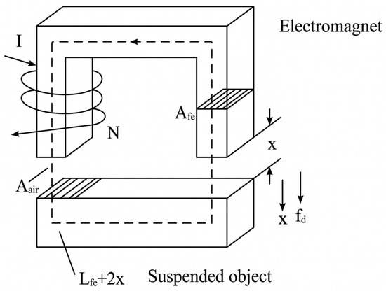
It is difficult to perform an accurate theoretical analysis of the magnetic circuit of an electromagnet. Therefore, a simplifying assumption is usually made that all magnetic flux passes through the iron core without leakage, except across the air gap, as shown in Fig-ure 13. In the figure, I denotes the excitation current of the suspension electromagnet coil; N represents the number of coil turns; A_fe is the cross-sectional area of the track iron core; A_ai is the equivalent cross-sectional area of the air gap; X represents the suspension air gap; f_d denotes the external disturbance load; and L_fe + 2x represents the total magnetic circuit length.

From Figure 13, the inductance of the electromagnet can be expressed as

$$L={\displaystyle \frac{{\mu }_0{N}^{2}A}{2x}}$$

(7)

Figure 13. Electromagnet magnetic circuit diagram.

If the effect of the iron core is neglected, the electromagnetic force can be expressed as

$$F={\displaystyle \frac{{\mu }_0{N}^2{I}^{2}A}{4x^2}}$$

(8)

When the cross-sectional area of the magnetic circuit is fixed, the magnitude of the electromagnetic force can be expressed by a closed-form formula. When the gravitational force acting on the levitation module equals the electromagnetic force, the control system reaches a balanced position, i.e., an equilibrium point. At equilibrium, $i=i_0$ and $z=z_0$. If an external disturbance occurs at equilibrium, a small displacement Δz is generated. Under this condition, the electromagnetic force is expressed as:

$$F={\displaystyle \frac{1}{4}}{\mu }_{0}NA{\displaystyle \frac{{(i_0+\Delta i)}^2}{{(z_0+\Delta z)}^2}}$$

(9)

At the equilibrium position, a Taylor series expansion of Equation (9) yields the following expression for the electromagnetic force:

$$F=F_0+{\displaystyle \frac{\partial F}{\partial \mathrm{z}}}z+{\displaystyle \frac{\partial F}{\partial i}}i=F_0+K_{z}z+K_{i}i$$

(10)

where $K_z={\displaystyle \frac{{\mu }_0{N}^{2}A{i_0}^2}{2{z_0}^3}}$ denotes the gap stiffness coefficient (N/m) and $K_i={\displaystyle \frac{{\mu }_0{N}^{2}A{i}_0}{2{z_0}^2}}$ denotes the current stiffness coefficient (A/m).

Based on Newton’s second law, the force analysis of the electromagnet yields the following mechanical equation:

$$m{\displaystyle \frac{d^{2}z}{d{t}^2}}=mg+f_d(t)-F(i,z)$$

(11)

The circuit equation of the electromagnet coil can be expressed as

$$U={\displaystyle \frac{d(LI)}{dt}}+RI$$

(12)

$$U=({\displaystyle \frac{{\mu }_0{N}^{2}A}{2x}})\cdot {\displaystyle \frac{dI}{dt}}-({\displaystyle \frac{{\mu }_0{N}^{2}AI}{2x^2}})\cdot {\displaystyle \frac{dx}{dt}}+RI$$

(13)

4.2. Control Model

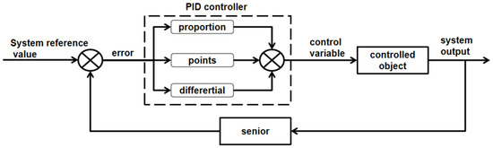
The block diagram of a PID control system is shown in Figure 14. The PID control determines the control signal based on the system error through proportional, integral, and derivative computations [33], expressed as

$$u(t)=K_p\left[e(t)+{\displaystyle \frac{1}{T_I}}{\displaystyle {\int }_0^{1}e(t)dt+T_D\frac{de(t)}{dt}}\right]$$

(14)

where $K_P$ denotes the proportional gain, $T_D$ denotes the derivative time constant, $T_I$ denotes the integral time constant, $u(t)$ denotes the control signal, and $e(t)$ represents the error between the controlled variable and the reference input.

Figure 14. PID control system block diagram.

The transfer function of the PID controller is given by

$$G(s)={\displaystyle \frac{U(s)}{E(s)}}=k_p+{\displaystyle \frac{k_i}{s}}+k_{d}s$$

(15)

Neglecting external disturbances and according to classical control theory, the transfer function between the levitation air gap and the applied voltage can be expressed as

$${\displaystyle \frac{z(s)}{U(s)}}=-{\displaystyle \frac{\frac{k_i}{m{L}_0}}{s^3+\frac{R}{L_0}{s}^2-\frac{k_{z}R}{m{L}_0}}}$$

(16)

For the open-loop system, the characteristic equation is

$$s^3+{\displaystyle \frac{R}{L_0}}{s}^2-{\displaystyle \frac{k_{z}R}{m{L}_0}}=0$$

(17)

According to the Routh–Hurwitz stability criterion, the open-loop system is unstable. Therefore, a feedback mechanism must be introduced to achieve system stability. The transfer function between voltage and current is

$${\displaystyle \frac{I(s)}{U(s)}}={\displaystyle \frac{1}{L_{0}s+R}}$$

(18)

From Equation (18), the time constant of the transfer function is $t={\displaystyle \frac{R}{L_0}}$. To address the delay effects between current and voltage within the system, a feedback circuit is introduced. After introducing current feedback, the transfer function in Equation (18) becomes

$${\displaystyle \frac{I(s)}{U(s)}}={\displaystyle \frac{K_1}{L_{0}s+K_1{K}_2+R}}$$

(19)

Taking the Laplace transform of Equation (10) yields

$$F_d(s)=m{s}^{2}z(s)+K_{z}z(s)+K_{i}I(s)$$

(20)

After transformation of Equation (20), the resulting output expression is

$$z(s)={\displaystyle \frac{f_d(s)-K_{i}I(s)}{m{s}^2+K_z}}$$

(21)

For simplification and under the assumption of negligible external disturbances, the system can be treated as a single-variable system, and the open-loop transfer function is obtained as

$${\displaystyle \frac{z(s)}{I(s)}}=-{\displaystyle \frac{K_i}{m{s}^2+K_z}}$$

(22)

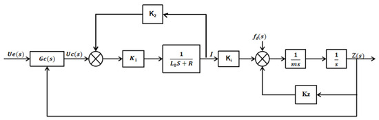
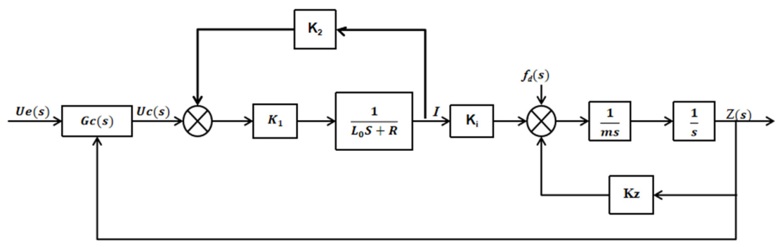
Similarly to voltage open-loop control, current open-loop control is also unstable. Therefore, feedback must be introduced to form a closed-loop system and to ensure proper control performance. In practice, combinations of feedback, such as position, velocity, acceleration, magnetic flux, and current, are commonly adopted. In this study, position feedback combined with current feedback is selected to control the levitation system, and the block diagram of the resulting closed-loop system [34] is shown in Figure 15.

Figure 15. Block diagram of the closed-loop system.

The transfer function of the PID control unit is expressed as follows:

$$G_c(s)={\displaystyle \frac{U_c(s)}{U_e(s)}}=k_p+{\displaystyle \frac{k_I}{s}}+{\displaystyle \frac{k_d}{1+t_{d}s}}$$

(23)

From Equation (23), it can be seen that, to enhance system stability and prevent abrupt changes in the derivative term, an inertia element $1/1+t_{d}s$ is introduced into the derivative component.

In summary, the closed-loop transfer function of the levitation control system is given by

$$G(s)={\displaystyle \frac{z(s)}{U(s)}}={\displaystyle \frac{K_i{G}_c(s)G_a(s)}{m{s}^2+k_z+k_i{G}_c(s)G_a(s)}}$$

(24)

where $G_a(S)$ represents the current feedback transfer function defined in Equation (19).

4.3. System Simulation

Based on the magnetic–track surrogate model and the levitation control algorithm described above, the control model and simulation analysis were implemented using MATLAB R2020a. During the simulation, system parameters were selected according to the actual design specifications, as listed in Table 3.

Table 3. System parameters.

Parameter	Symbol	Value	Unit
Suspension block mass	m	729.65	Kg
Coil turns	N	320	circle
Suspension gap	z0	8	mm
Coil resistance	R	0.55	Ω
Rated current	I	25	A
Effective coil area	A	0.01848	m2
Air permeability	μ0	4π × 10−7	H/m

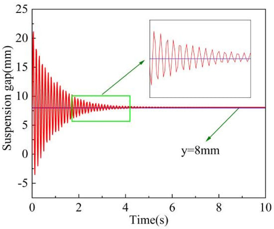
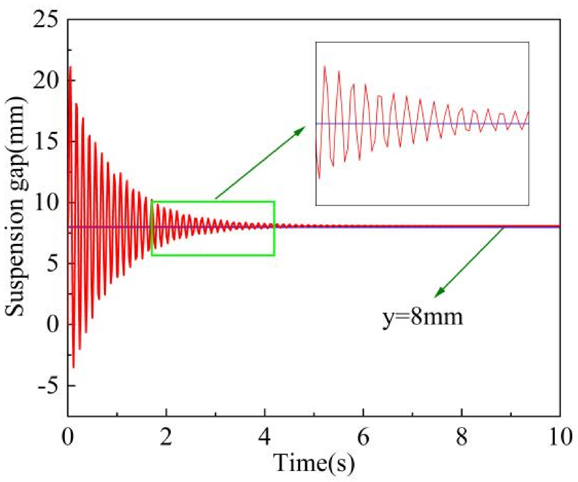
By tuning the PID control parameters, suitable levitation control gains were obtained, and their variation is shown in Figure 16. As illustrated in the figure, the levitation gap exhibits significant oscillations at the initial stage [38]; however, it gradually stabilizes near the nominal levitation gap of 8 mm after approximately 4 s. The nominal levitation gap represents the rated operating gap of the maglev train and is compared with the final simulation output of the levitation control model.

Figure 16. Fluctuation curve of the suspension gap in the control model.

In conclusion, this study developed a PID-based control model and integrated it with the magnetic–track electromagnetic force surrogate model, thereby establishing a complete levitation control framework for the vehicle.

5. Dynamic Coupling Model of Maglev Vehicle and Track

5.1. Vehicle–Track Coupling Model

The maglev vehicle mainly consists of the car body, running gear, and levitation system. The running gear includes suspension frames, a secondary suspension system, and forced-guidance mechanisms. Each vehicle is equipped with five suspension frames evenly distributed beneath the car body, and each frame connects the left and right modules through an anti-roll beam. The complete vehicle model has 154 degrees of freedom, and the dynamic flow of the vehicle–track coupling system is illustrated in Figure 17.

Figure 17. Flowchart of the vehicle–track coupling system.

The main parameters used in the vehicle dynamic modeling process are listed in Table 4.

Table 4. Main parameters of the kinetic model.

Parameter	Value	Unit
Track gauge	1.86	m
Number of suspension frames	5	one
Rated suspension gap	8	mm
Vehicle body mass	12,490	kg
Suspension module mass	729.65	kg
Longitudinal stiffness of secondary suspension spring	2,600,000	N/m
Lateral stiffness of secondary suspension spring	2,600,000	N/m
Vertical stiffness of secondary suspension spring	66,000	N/m

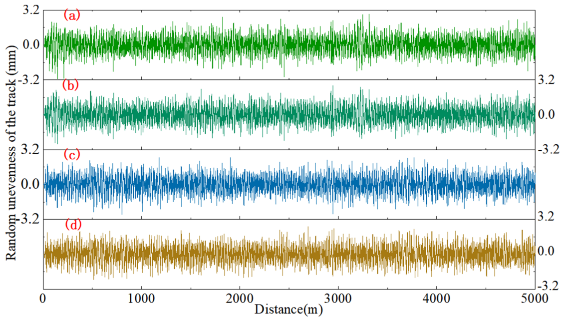
Because the current operating mileage of medium- and low-speed maglev systems is relatively limited, measured data on track irregularities are scarce. Figure 18 shows the reconstructed track irregularity profile derived from the random irregularity spectrum theory for flexible elevated guideways and the track precision requirements specified in CJJ/T 262—2017 Design Code for Medium- and Low-Speed Maglev Transit [53].

Figure 18. Track irregularities. (a) Vertical left rail (b) Vertical right rail (c) Horizontal left rail (d) Lateral right rail.

5.2. Validation of the Dynamic Model

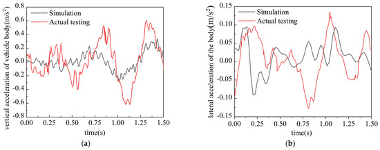
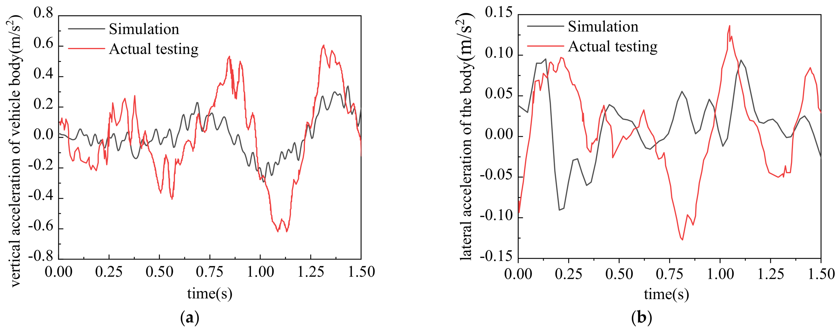
Because a complete set of measured data on the lateral system response of maglev vehicles passing through turnouts is currently unavailable, the dynamic response of the car body at a speed of 140 km/h was compared with measured car-body response data obtained from a maglev test line at a specific location [36] to ensure the accuracy and reliability of the calculations. Figure 19 compares the simulation results with the measured data.

Figure 19. Comparison between simulation results and measured data: (a) car-body vertical acceleration; (b) car-body lateral acceleration.

As shown in Figure 19, the comparison between the simulated and measured vibration accelerations of the car body indicates that the model developed in this study closely matches the experimental data under track irregularity excitation. Although minor discrepancies exist due to differences in the amplitudes of track irregularities, they remain within acceptable limits. These results demonstrate that the proposed model is reliable and suitable for subsequent dynamic simulations and analyses.

6. Effect of Levitation Faults on Vehicle Performance

6.1. Levitation Failure During Operation

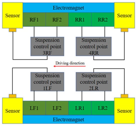
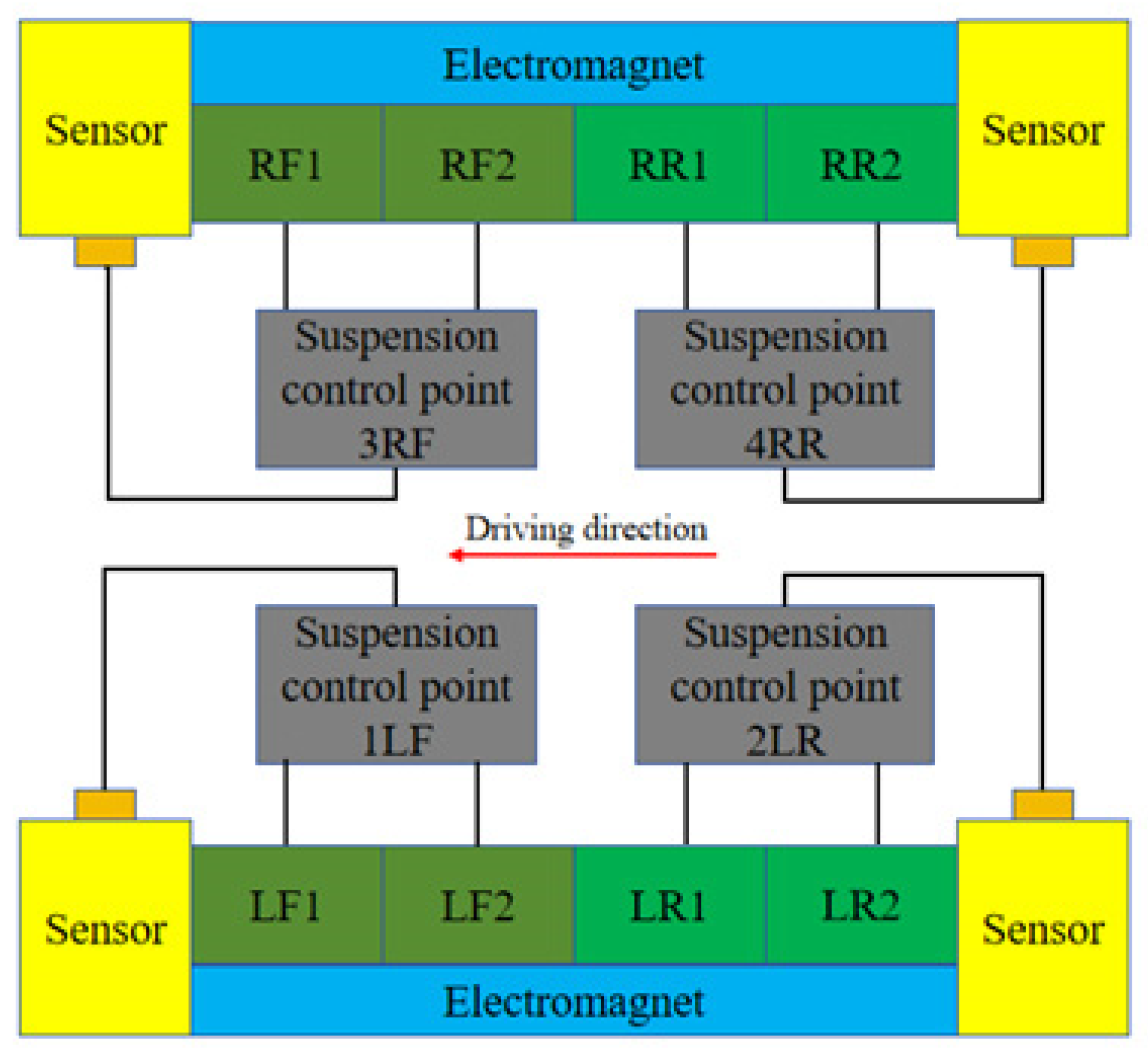
Figure 20 shows a schematic of the vehicle levitation control system. Each suspension frame is equipped with two electromagnets on the left and right sides, and each electromagnet contains four magnetic poles (LF-Left Front, LR-Left Rear, RF-Right Front, RR-Right Rear). Two adjacent poles form one levitation control point, so each suspension frame has four levitation control points in total. Fault analysis was conducted with respect to these control points.

Figure 20. Schematic of suspension control.

The third suspension frame of the vehicle was selected for study. The dynamic performance of the vehicle was analyzed under one-point, two-point (same side and opposite sides), and three-point levitation fault conditions.

6.1.1. Single-Point Levitation Fault

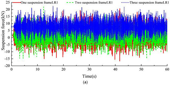
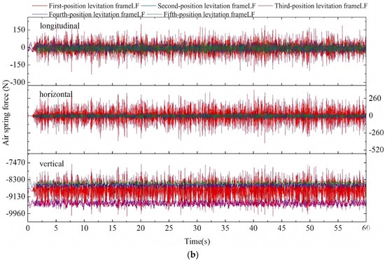
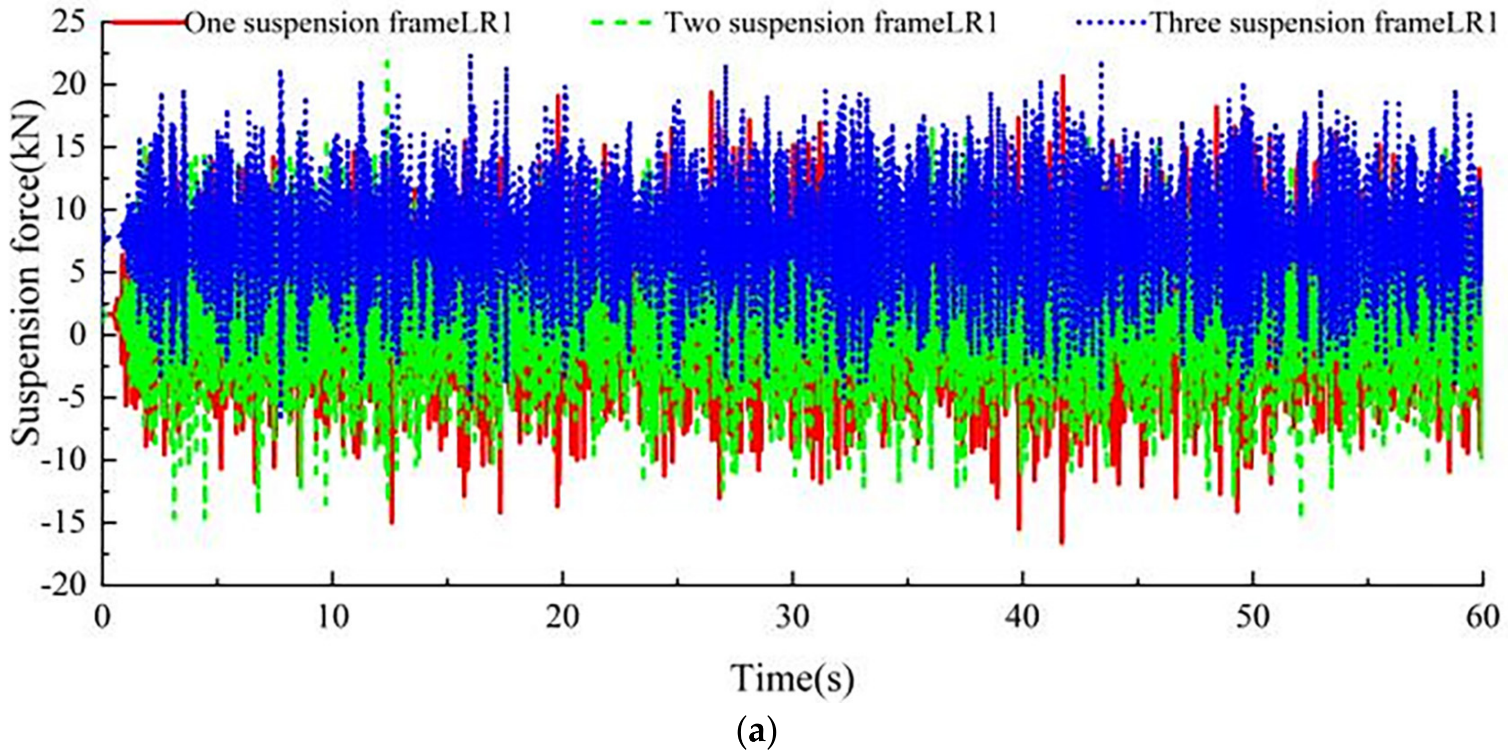
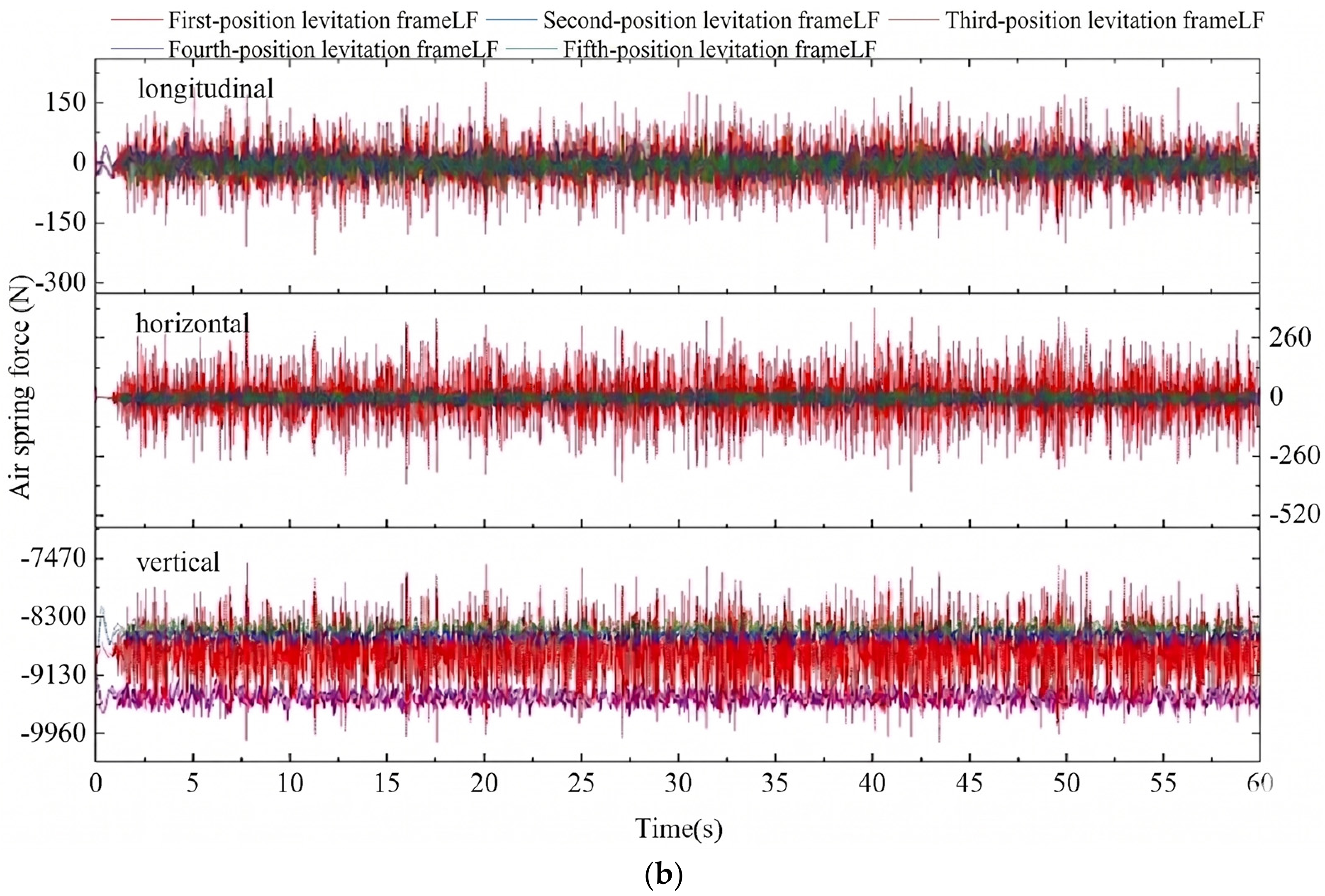
When a levitation fault occurs at the LF levitation point of the third suspension frame in the middle car while the train operates at 80 km/h, the LR electromagnet on the same side exhibits variations in levitation force, and the air springs of the first three suspension frames show corresponding reaction forces (Figure 21).

Figure 21. Single suspension point failure: (a) time-history curve of levitation force at LR during levitation point failure at LF; (b) time-history curve of air-spring force during suspension point failure at LF.

As shown in Figure 21a, when the LF electromagnet of the third suspension frame fails, the levitation force of the LR electromagnet on the same side increases correspondingly, while the levitation forces of other suspension frames show no significant change. Figure 21b indicates that, upon LF electromagnet failure of the third suspension frame, the vertical, longitudinal, and lateral forces of the corresponding air spring all increase, and the amplitude of their fluctuations becomes significantly larger. According to Q/CRCC 32803–2019 Design Specification for Medium- and Low-Speed Maglev Transit, the maximum levitation capacity for commercial-operation vehicles in China should not be less than 25 kN/m. This aligns with the results shown in Figure 21a, indicating that if the wear resistance of the landing skids remains within the standard range, the train can operate at a reduced speed in the event of a single-point levitation fault, allowing it to clear passengers and return safely to the depot for maintenance.

6.1.2. Two-Point Levitation Faults (Same Side)

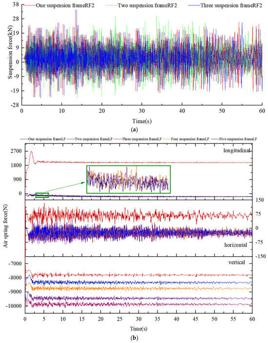
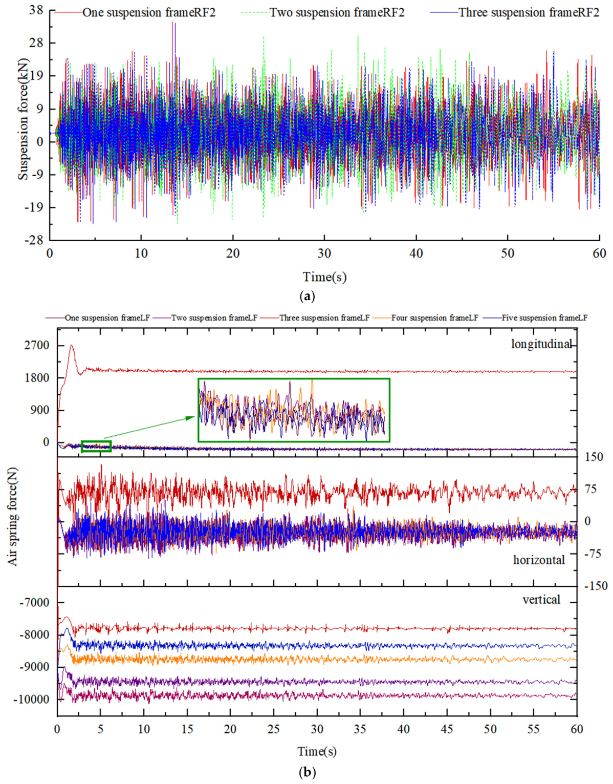
When both the LF and LR levitation points on the left side of the third suspension frame fail simultaneously, the right-side electromagnets on the first three suspension frames exhibit a variation in levitation force (Figure 22a). The air-spring forces corresponding to the failed left-side electromagnets of the third suspension frame also vary (Figure 22b).

Figure 22. Two suspension point failures (same side): (a) time-history curve of suspension force during LF and LR suspension point failures; (b) time-history curve of air-spring force during left suspension point failure.

As shown in Figure 22a, the stable levitation force amplitude of a single point is approximately 18 kN. However, when two levitation points on the same side fail simultaneously, the amplitude increases to about 28 kN. This indicates that the failure of the left-side levitation points on the third suspension frame causes a significant increase in the overall fluctuation of levitation force within the vehicle system. As shown in Figure 22b, when two levitation points on the same side of a suspension frame fail, the longitudinal, lateral, and vertical forces acting on the air spring increase significantly. The longitudinal force of the air spring on the faulty suspension frame is opposite in direction to that of the normally functioning frames. This occurs because the failure of both levitation points on one side causes the suspension frame to tilt toward the failed side, leading to a substantial increase in air-spring load and a reversal of its longitudinal force direction relative to other air springs.

6.1.3. Two-Point Levitation Faults (Opposite Sides)

When the LF and RF levitation points of the third suspension frame fail simultaneously, the LR points of the first three suspension frames exhibit variations in levitation force (Figure 23a), and the LF air springs of each suspension frame show corresponding reaction forces (Figure 23b).

Figure 23. Two suspension point failures (opposite sides): (a) time-history curve of suspension force during suspension point failures on opposite sides; (b) time-history curve of air-spring force during suspension point failures on opposite sides.

As shown in Figure 23a, when two levitation points—LF and RF—of the third suspension frame fail, the remaining levitation points on that frame do not share the levitation load evenly. Instead, their individual levitation forces increase sharply, reaching several times the normal level. Moreover, under two-point fault conditions, the fluctuation amplitudes of levitation forces increase on both faulty and non-faulty suspension frames, with the affected frame exhibiting much stronger oscillations. This demonstrates that simultaneous failures of two levitation points on a single suspension frame cause rapid increases and severe oscillations in levitation force, which adversely affect the dynamic performance of the vehicle system. As shown in Figure 23b, the longitudinal, lateral, and vertical air-spring forces on the third suspension frame fluctuate far more than on other frames. This indicates that when one levitation point on each side of a suspension frame fails, the air-spring forces in all three directions—longitudinal, lateral, and vertical—increase substantially.

6.1.4. Three-Point Levitation Faults

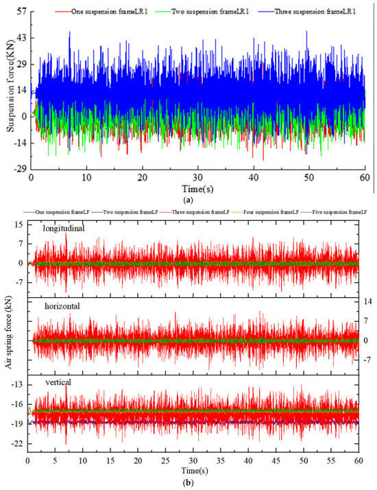
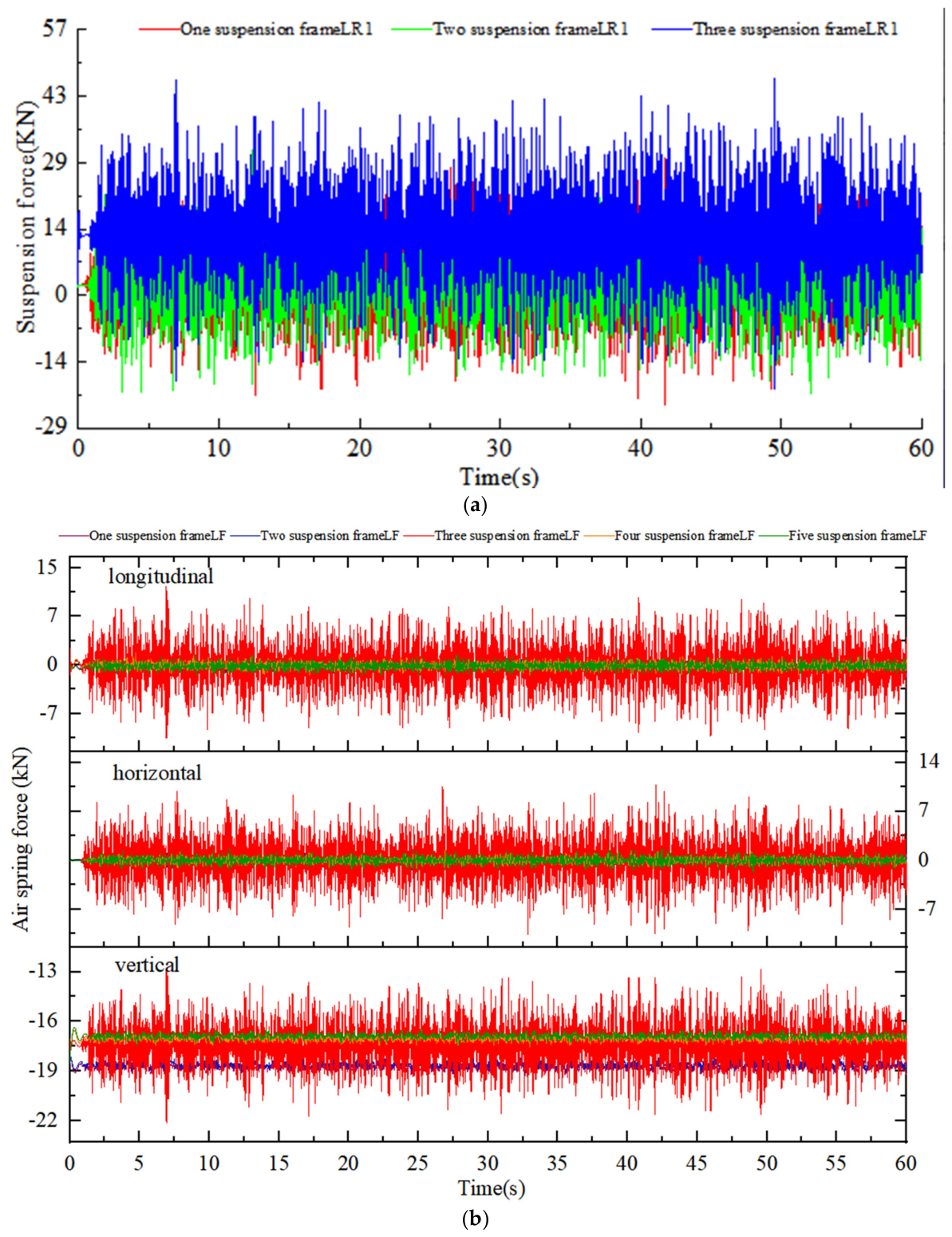
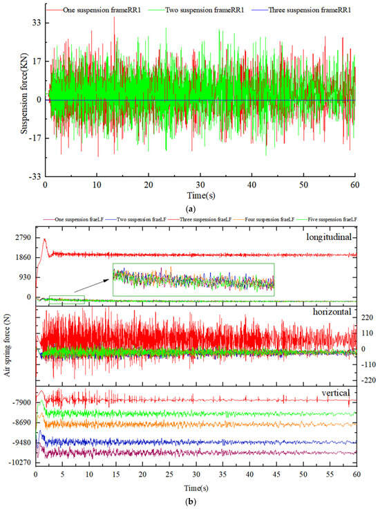
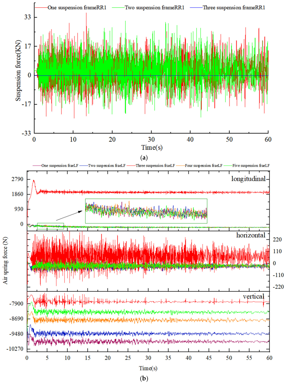
When three levitation points—LF, LR, and RF—of the third suspension frame fail simultaneously, the RR points of the first three suspension frames exhibit variation in levitation force (Figure 24a), and the air-spring forces show corresponding reaction forces under three-point failure conditions (Figure 24b).

Figure 24. Three suspension point failures: (a) time-history curve of suspension force during three suspension point failures; (b) time-history curve of air-spring force during three suspension point failures.

Figure 24a shows that levitation point failures cause significant increases in the levitation force fluctuations of other suspension frames. When all three levitation points (LF, LR, and RF) of the third suspension frame fail, the remaining levitation point cannot sustain normal operation; its levitation force drops to zero, causing the suspension frame to lose levitation and fall onto the track. Figure 24b shows that under the same three-point failure conditions, the longitudinal, lateral, and vertical forces of the air spring on the third suspension frame are significantly greater than those on other frames.

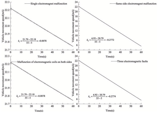
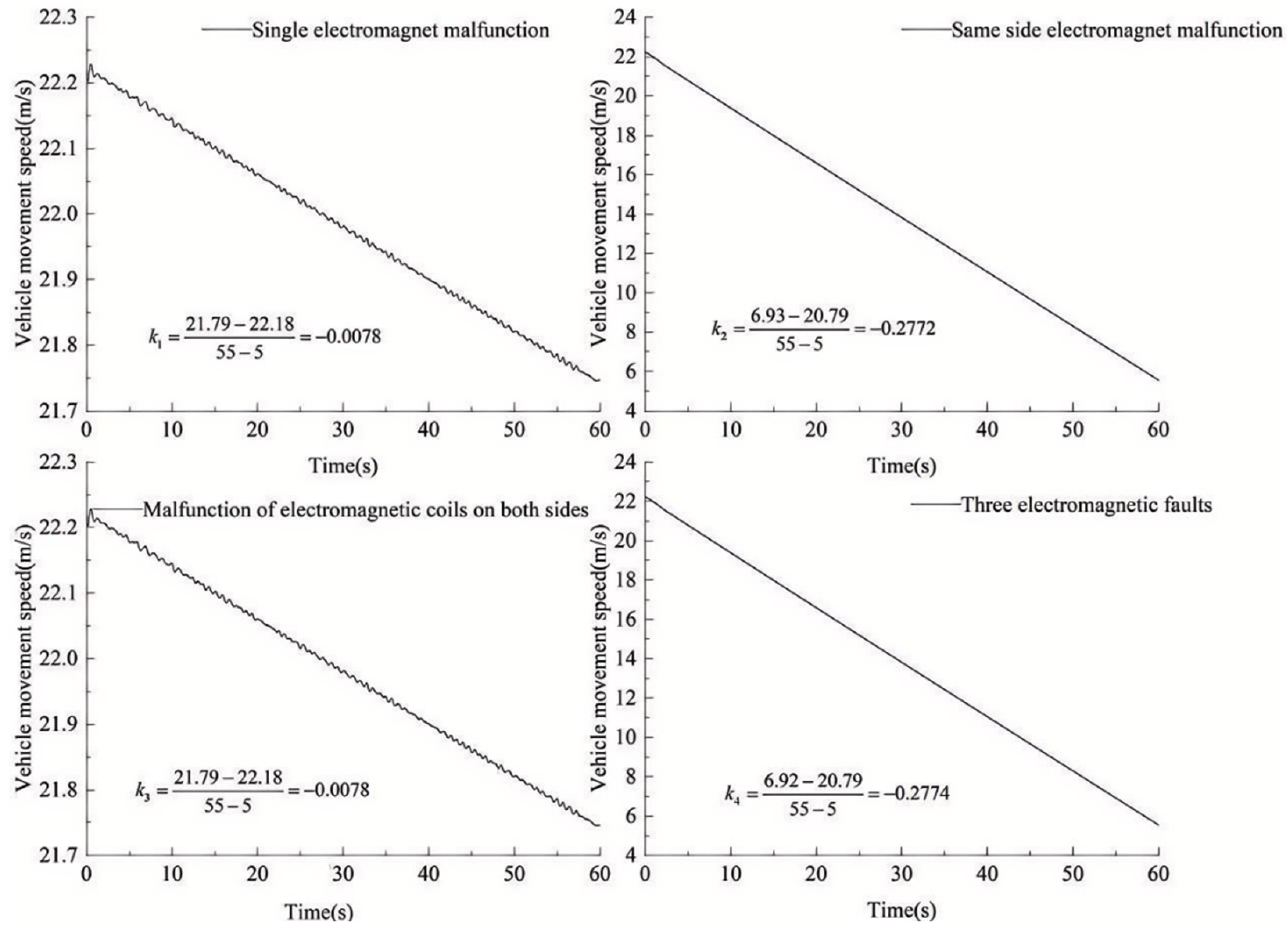
Figure 25 shows the variations in vehicle speed under different levitation point failure conditions at a nominal speed of 80 km/h.

Figure 25. Time-history curve of vehicle operating speed under different suspension point failures.

As shown in Figure 25, in the absence of emergency braking or other protective measures, any single levitation point failure causes a decrease in vehicle speed. The speed variations caused by a single-point fault on one side and by one fault on each side are almost identical. In contrast, the speed variations caused by two same-side point faults are nearly identical to those caused by three-point faults on the same suspension frame. When only one levitation point fails, or when one point on each side fails, the remaining functional points on the suspension frame still provide sufficient levitation force to maintain movement. However, when two same-side levitation points fail, the electromagnet on that side detaches from the guideway, resulting in faster deceleration. When three points fail, the entire suspension frame detaches from the guideway, causing a sharp drop in speed.

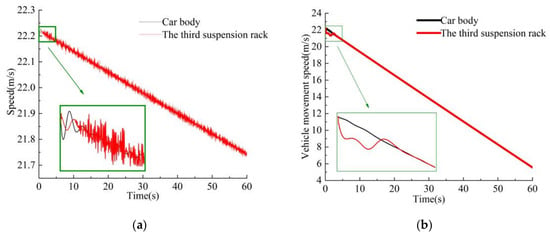
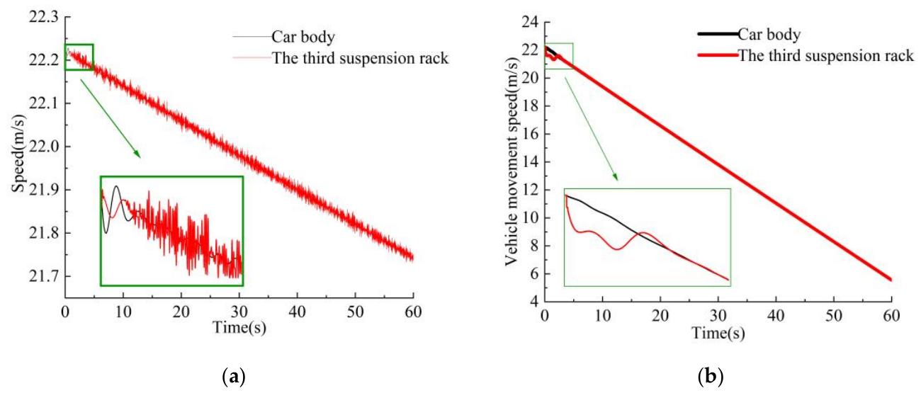
Therefore, the vehicle’s motion characteristics are essentially the same for single-point faults on one side and for one-point faults on each side, while the effects of two same-side faults are comparable to those of three-point faults on the same suspension frame. Figure 26 presents the velocity variation curves of the vehicle body and the third suspension frame under single same-side point fault and two same-side point fault conditions. As shown in the figure, when a single levitation point on one side fails, the longitudinal velocity of the affected suspension frame exhibits strong fluctuations. In contrast, when two same-side points fail, both the vehicle and the suspension frame undergo nearly uniform deceleration.

Figure 26. Velocity variation in the vehicle body and suspension frame: (a) single suspension point failure on one side; (b) two suspension point failures on the same side.

In summary, levitation point failures cause significant fluctuations in both levitation and air-spring forces. Single-point or opposite-side faults have a smaller impact on the vehicle’s dynamic performance than same-side faults, which cause the affected suspension frame to tilt and reduce overall dynamic stability. When three levitation points on a suspension frame fail, the remaining operational point cannot sustain the load, resulting in a complete loss of levitation for that frame.

6.2. Electromagnet Lock-Up (Saturation Adhesion)

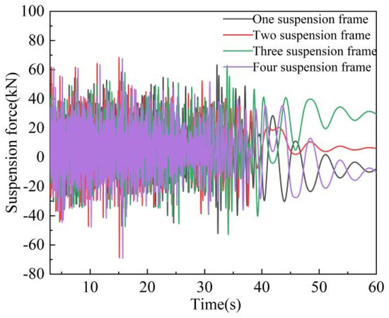
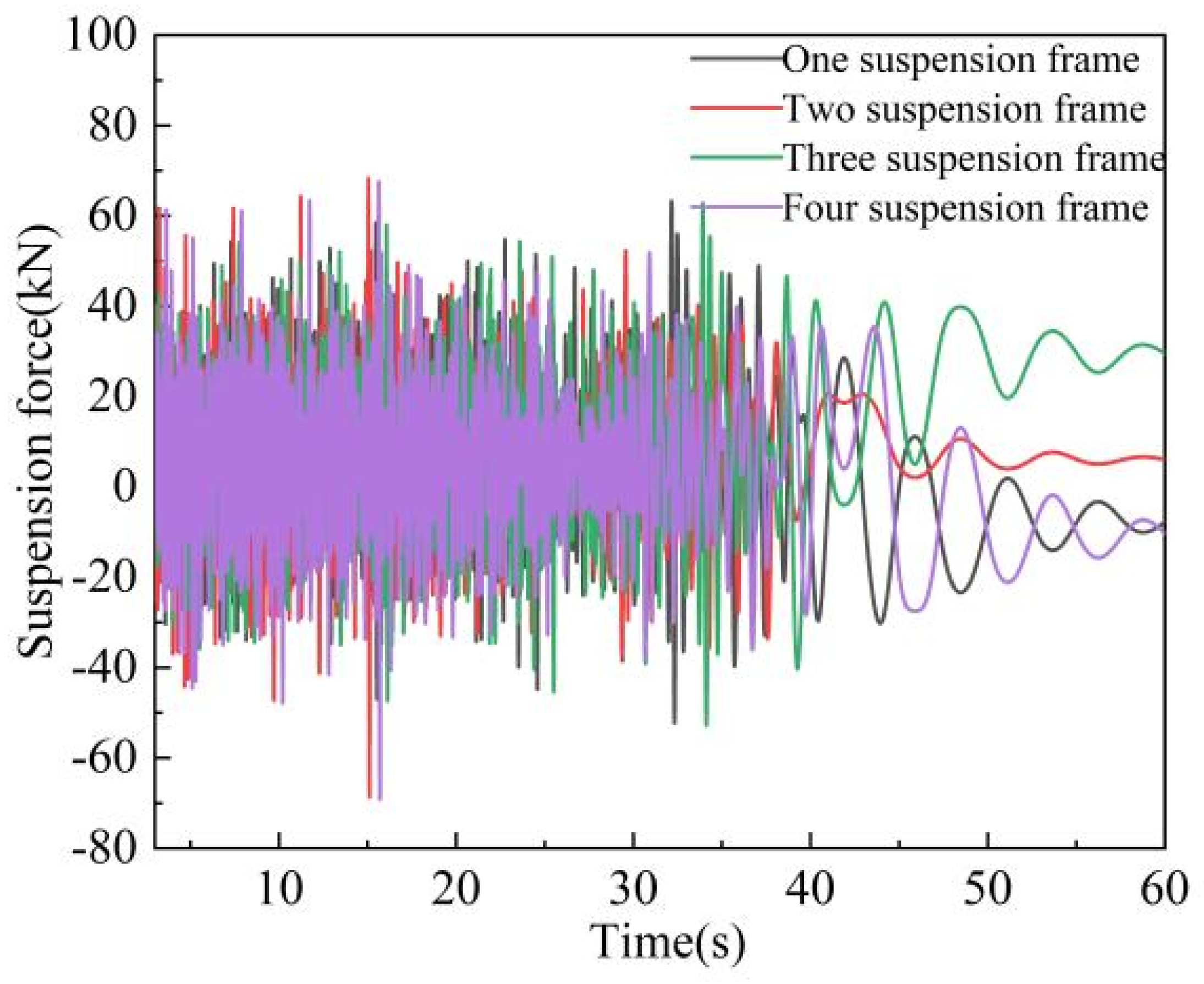
During normal operation, instability in the levitation control system may cause an electromagnet lock-up phenomenon. When the electromagnet of the third suspension frame locks up while the train runs at 80 km/h on a straight track, the levitation forces of other suspension frame electromagnets vary, as shown in Figure 27.

Figure 27. Variation in suspension force when the electromagnet is stuck.

Figure 27 shows that when the third suspension frame electromagnet locks up at 80 km/h on a straight track, the levitation force experiences a sudden and sharp increase. Compared with the normal levitation condition, where a single-point levitation force is about 18 kN, the instantaneous force during lock-up rises to approximately three times that value. If the electromagnet remains locked for a certain duration, the vehicle will eventually stop.

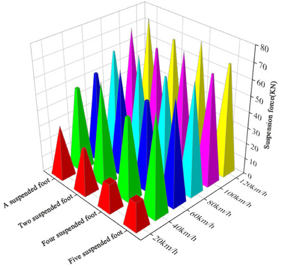
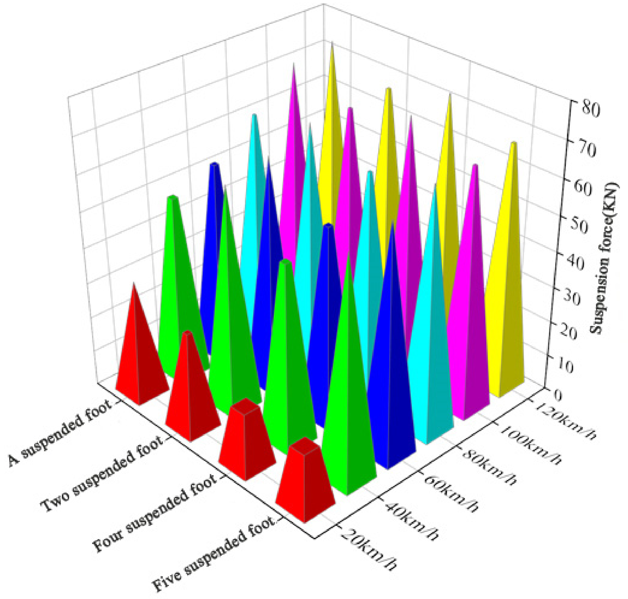
To illustrate the effect of speed on electromagnet lock-up, Figure 28 shows the maximum levitation force under lock-up conditions at different vehicle speeds.

Figure 28. Electromagnetic Levitation Force under Different Operating Speeds.

Figure 28 shows that when the third suspension frame electromagnet locks up at different vehicle speeds, the instantaneous maximum levitation force increases markedly with speed, indicating that lock-up at higher speeds has a greater impact and poses a serious threat to the vehicle’s performance and safety.

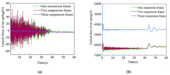
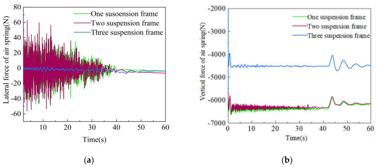
When the third suspension frame electromagnet locks up at 80 km/h, the air-spring reaction forces at the LF positions of the first three suspension frames vary, as shown in Figure 29.

Figure 29. Air-spring forces: (a) lateral force; (b) vertical force.

Based on the analysis of Figure 29, it can be observed that under different operating speeds, when an electromagnet “sucking death” fault occurs at the third levitation frame of the vehicle, the instantaneous maximum value of the levitation force increases significantly with the rise in speed. This indicates that the “sucking death” fault poses a more severe threat to the overall performance of the vehicle under high-speed operating conditions. Therefore, it is imperative to prioritize fault protection and speed-limiting redundancy for high-speed scenarios in the control strategy.

Moreover, the “sucking death” fault disrupts the original load distribution and guidance constraint capabilities of the levitation system, causing the entire vehicle’s levitation and suspension systems to enter a state of asymmetric force distribution. Consequently, in fault diagnosis and fault-tolerant control, it is not only necessary to monitor the impact amplitude at the “sucking death” point itself but also to pay attention to its cascading fluctuation effects on the air springs of adjacent levitation frames. Additionally, a lateral stability compensation or active intervention threshold should be set in response to the phenomenon where the lateral force approaches zero to prevent the vehicle from experiencing lateral instability or rollover risks.

7. Conclusions

Based on vehicle–track coupled dynamics theory and considering the spatial dynamic maglev–track relationship alongside the levitation control system, this paper analyzes the effects of levitation electromagnet failures on maglev vehicle performance. The main conclusions are as follows:

●

Significant discrepancies exist between the theoretically calculated electromagnetic forces and the simulation results due to the simplifying assumptions used in theory. To address this, a spatial dynamic maglev–track relationship model accounting for magnetic leakage and saturation effects was established.

●

Because ferromagnetic materials exhibit magnetic saturation, the increase in the simulated levitation force slows as coil current rises. Comparison of the simulated and theoretical guidance forces under varying levitation gaps shows that the results converge at larger air gaps. Smaller air gaps exacerbate magnetic flux leakage, amplifying the influence of the levitation gap on the guidance force.

●

Among the four operating conditions analyzed, lateral displacement has the most significant effect on levitation force, while rolling causes only minor variations (within 500 N). For the guidance force, noticeable changes occur only during lateral displacement and yawing, increasing as the displacement and yaw angle grow.

●

Levitation electromagnet failures induce pronounced fluctuations in levitation force, air-spring forces, and vehicle vibration acceleration. A fault in one magnetic pole of a levitation point has a smaller impact on vehicle performance than failure of an entire module, since the remaining pole can still provide sufficient levitation force.

●

Opposite-side levitation point failures are less severe than same-side module failures, as same-side faults cause the suspension frame to tilt and degrade overall dynamic performance. When three levitation modules on one suspension frame fail, the levitation forces of other suspension frames increase and fluctuate more intensely. The remaining single functional levitation point cannot support the frame, causing it to lose levitation and slide along the track, supported only by the skid.

●

Electromagnet lock-up in a suspension frame causes large fluctuations in levitation force, vehicle vibration acceleration, and air-spring forces. The instantaneous levitation force of the remaining suspension frames increases with vehicle speed, and severe lock-up can damage components and significantly compromise both vehicle and track safety.

References

- Zhai, W.M.; Zhao, C.F. Maglev vehicle/track system dynamics (I)—Mag/track interaction and stability. J. Mech. Eng. 2005, 41, 1–10. [Google Scholar] [CrossRef] [Scilit]
- Brzezina, W.; Langerholc, J. Lift and side forces on rectangular pole pieces in two dimensions. J. Appl. Phys. 1974, 45, 1869–1872. [Google Scholar] [CrossRef] [Scilit]
- Cui, P.; Zhang, K.; Li, J. Analytical calculation of suspension electromagnet force and torque based on Schwarz-Christoffel transformation. Proc. CSEE 2010, 30, 129–134. [Google Scholar]
- Xie, Y.D.; Chang, W.S. Calculation of single electromagnet force for EMS maglev and study on motion stability and controllability. J. China Railw. Soc. 1995, 17, 41–48. [Google Scholar]
- Sinha, P.K. Electromagnetic Suspension Dynamics & Control; Magnetic Levitation Vehicles; Institution of Electrical Engineers: New York, NY, USA, 1987. [Google Scholar]
- Cui, P.; Li, J.; Liu, D.S. Calculation of load-bearing capacity of normally conductive low-speed maglev trains on curves. Cientia Sin. (Technol.) 2010, 40, 772–777. [Google Scholar]
- Zhang, G.; Li, J.; Li, J.H. Kinematics research on anti-rolling suspension rods of low-speed maglev trains. J. China Railw. Soc. 2012, 34, 28–33. [Google Scholar]
- Shi, J.; Wei, Q.C. Research on maglev rail relationship of normally conductive maglev railway. J. North. Jiaotong Univ. 2004, 28, 41–44. [Google Scholar]
- Zhao, C.F.; Zhai, W.M. Maglev vehicle/track system dynamics (II)—Modeling and simulation. J. Mech. Eng. 2005, 41, 163–175. [Google Scholar] [CrossRef] [Scilit]
- Fan, Y.L. Research on the Influence of Maglev Rail Relationship on Vertical Dynamics of Medium-Low Speed Maglev Systems. Master’s Thesis, Southwest Jiaotong University, Chengdu, China, 2020. [Google Scholar]
- He, G. Dynamics Modeling and Guidance Capability Research of EMS Medium-Speed Maglev Trains. Ph.D. Thesis, National University of Defense Technology, Changsha, China, 2016. [Google Scholar]
- Wen, J.L. Research on Five-Degree-of-Freedom Maglev Rail Relationship of Suspension Electromagnets for Maglev Trains. Master’s Thesis, National University of Defense Technology, Changsha, China, 2015. [Google Scholar]
- Zeng, S. Spatial Maglev Rail Relationship and its Application in Dynamics of Medium-Low Speed Maglev Trains. Master’s Thesis, National University of Defense Technology, Changsha, China, 2017. [Google Scholar]
- Liang, X.; Luo, S.H.; Ma, W.H. Research on dynamic maglev rail relationship of normally conductive maglev trains. J. China Railw. Soc. 2013, 35, 39–45. [Google Scholar]
- Liang, X.; Ma, W.H. Comparative analysis of maglev vehicle-bridge interaction based on two types of maglev rail relationships. J. Railw. Sci. Eng. 2017, 14, 845–851. [Google Scholar]
- Wang, Z.Y.; Ma, W.H.; Luo, S.H.; Wang, B.; Wang, A.; Zhang, X. Influence of maglev rail relationship modeling on high-speed maglev dynamics simulation. Machinery 2023, 50, 31–37. [Google Scholar]
- Tian, W.J. Research on Electromagnetic Characteristics of Suspension Electromagnets for Two Typical Medium-Low Speed Maglev Trains. Master’s Thesis, National University of Defense Technology, Changsha, China, 2009. [Google Scholar]
- Chen, G.R.; Chang, W.S.; Yin, L.M. Design and research of suspension electromagnets for maglev trains. J. Natl. Univ. Def. Technol. 1993, 15, 10–15. [Google Scholar]
- Li, Y.G.; Zhang, X.; Long, J.; Liu, H. Research on U-shaped electromagnet design method for EMS low-speed maglev trains. J. Natl. Univ. Def. Technol. 2011, 33, 159–162+168. [Google Scholar]
- Wang, Z.L.; Xu, Y.L.; Li, G.Q.; Chen, S.W.; Zhang, X.-L. Dynamic analysis of a coupled system of high-speed maglev train and curved viaduct. Int. J. Struct. Stab. Dyn. 2018, 18, 18504132. [Google Scholar] [CrossRef] [Scilit]
- Zhao, Z.W.; Xu, S.; Liu, K.; Yang, W.; Li, J.; Ma, G. 3-D analytical model of racetrack HTS coil subject to travelling magnetic fields. J. Supercond. Nov. Magn. 2020, 34, 75–84. [Google Scholar] [CrossRef] [Scilit]
- Takinami, A.H.; Cruz, R.B.; de Lima, B.L.S.; de Almeida, F.J. Design, simulation and development of a magnetic levitation system (MAGLEV). Results Phys. 2020, 17, 103115. [Google Scholar] [CrossRef] [Scilit]
- Aloisio, A.; De Angelo, M.; Alaggio, R.; D’OVidio, G. Dynamic identification of hts maglev module for suspended vehicle by using a single-degree-of-freedom generalized Bouc-Wen hysteresis model. J. Supercond. Nov. Magn. 2021, 34, 399–407. [Google Scholar] [CrossRef] [Scilit]
- Wang, X.P.; Li, G.F.; Mu, X.L.; Wang, H.; Jin, Z.; Ding, W. Dynamic response analysis of medium-low speed maglev vehicle-track coupling system in small radius curves. J. Vib. Shock. 2022, 41, 81–89105. [Google Scholar]
- Feng, Y.; Zhao, C.F.; Bai, Z.; Tong, L.S.; Shu, Y. A modified electromagnetic force calculation method has high accuracy and applicability for EMS maglev vehicle dynamics simulation. ISA Trans. 2023, 137, 186–198. [Google Scholar] [CrossRef] [Scilit]
- Liu, Y.; Deng, W.; Gong, P. Dynamics of the bogie of maglev train with distributed magnetic forces. Shock. Vib. 2015, 2015, 896410. [Google Scholar] [CrossRef] [Scilit]
- Liu, S.K.; An, B.; Liu, S.; Guo, Z.J. Characteristic research of electromagnetic force for mixing suspension electromagnet used in low-speed maglev train. IET Electr. Power Appl. 2015, 9, 223–228. [Google Scholar] [CrossRef] [Scilit]
- Suebsomran, A. Optimal control of electromagnetic suspension EMS system. Open Autom. Control. Syst. J. 2014, 6, 1–8. [Google Scholar] [CrossRef] [Scilit]
- Chen, Q.; Li, X.L.; Liu, S.K. Nonlinear PID control of suspension system for maglev trains. Electr. Drive Locomot. 2014, 52–54. [Google Scholar]
- Feng, Y.; Zhao, C.F.; Liang, X.; Jiang, Z.C. Influence of bolster-hanger length on the dynamic performance of high-speed EMS maglev vehicles. Veh. Syst. Dyn. 2022, 60, 3743–3764. [Google Scholar] [CrossRef] [Scilit]
- Shi, Y.; Ma, W.H.; Li, M.; Xu, Z.Q. Research on dynamics of a new high-speed maglev vehicle. Veh. Syst. Dyn. 2022, 60, 721–742. [Google Scholar] [CrossRef] [Scilit]
- Zhang, L.L. Vibration analysis and multi-state feedback control of maglev vehicle-guideway coupling system. Electron. Res. Arch. 2022, 30, 3887–3901. [Google Scholar] [CrossRef] [Scilit]
- Han, J.B.; Han, H.S.; Lee, J.M.; Kim, S.S. Dynamic modeling and simulation of EMS maglev vehicle to evaluate the levitation stability and operational safety over an elastic segmented switch track. J. Mech. Sci. Technol. 2018, 32, 2987–2998. [Google Scholar] [CrossRef] [Scilit]
- Liang, X.; Jiang, T.Y.; Hong, Y.; Zhang, J.; Jiang, M.; Wang, Z. Vibration response analysis of simply supported box girder bridge-maglev train in accelerated test of Changsha maglev express. Adv. Mater. Sci. Eng. 2020, 2020, 9563747. [Google Scholar] [CrossRef] [Scilit]
- Han, X.H.; Li, Z.J.; Chi, M.R. Influence of track beam structure on vehicle-track coupling vibration of medium-low speed maglev. Railw. Locomot. Car 2019, 39, 36–42. [Google Scholar]
- Sun, Y.G.; Xu, J.Q.; Qiang, H.Y.; Chen, C.; Lin, G. Adaptive sliding mode control of maglev system based on RBF neural network minimum parameter learning method. Measurement 2019, 141, 217–226. [Google Scholar] [CrossRef] [Scilit]
- Sun, Y.G.; Xu, J.Q.; Chen, C.; Hu, W. Reinforcement learning-based optimal tracking control for levitation system of maglev vehicle with input time delay. IEEE Trans. Instrum. Meas. 2022, 71, 1–13. [Google Scholar] [CrossRef] [Scilit]
- Sun, Y.G.; Wang, S.M.; Lu, Y.; Xu, J. Gaussian process dynamic modeling and backstepping sliding mode control for magnetic levitation system of maglev train. J. Theor. Appl. Mech. 2022, 60, 49–62. [Google Scholar] [CrossRef] [Scilit]
- Zhou, D.F.; Li, J.; Zhang, K. Amplitude control of the track-induced self-excited vibration for a maglev system. ISA Trans. 2014, 53, 1463–1469. [Google Scholar] [CrossRef] [Scilit]
- Zhou, D.F.; Yu, P.C.; Wang, L.C.; Li, J. An adaptive vibration control method to suppress the vibration of the maglev train caused by track irregularities. J. Sound Vib. 2017, 408, 331–350. [Google Scholar] [CrossRef] [Scilit]
- Chen, C.; Xu, J.Q.; Lin, G.B.; Sun, Y.; Zhao, X. Sliding mode bifurcation control based on acceleration feedback correction adaptive compensation for maglev train suspension system with time-varying disturbance. IEEE Trans. Transp. Electrif. 2022, 8, 2273–2287. [Google Scholar] [CrossRef] [Scilit]
- Chen, C.; Xu, J.Q.; Rong, L.J.; Ji, W.; Lin, G.; Sun, Y. Neural-network-state-observation-based adaptive inversion control method of maglev train. IEEE Trans. Veh. Technol. 2022, 71, 3660–3669. [Google Scholar] [CrossRef] [Scilit]
- Su, X.Y.; Xu, Y.L.; Yang, X.F. Neural network adaptive sliding mode control without overestimation for a maglev system. Mech. Syst. Signal Process. 2022, 168, 108661. [Google Scholar] [CrossRef] [Scilit]
- Yaseen, H.M.S.; Siffat, S.A.; Ahmad, I.; Malik, A.S. Nonlinear adaptive control of magnetic levitation system using terminal sliding mode and integral backstepping sliding mode controllers. ISA Trans. 2022, 126, 121–133. [Google Scholar] [CrossRef] [Scilit]
- Wen, T.; Long, Z.Q.; Zhou, X.; Malik, A.S. Study on data-driven control of maglev train levitation system based on Koopman linear reconstruction. Proc. Rom. Acad. Ser. A-Math. Phys. Tech. Sci. Inf. Sci. 2022, 23, 161–170. [Google Scholar]
- Zhai, M.D.; Li, X.L.; Long, Z.Q.; Dou, F. Control and optimization design of suspension system for high-speed maglev trains based on Youla parameterization. J. Tongji Univ. (Nat. Sci. Ed.) 2023, 51, 341–350. [Google Scholar]
- Cui, Y.H.; Guo, X.R.; Mao, H.W.; Liu, J. Research on the Dynamic Characteristics of a Typical Medium–Low-Speed Maglev Train–Bridge System Influenced by the Transverse Stiffness of Pier Tops. Appl. Sci. 2025, 15, 6628. [Google Scholar] [CrossRef] [Scilit]
- Sun, Y.G.; Li, F.X.; Zhang, Z.; Gao, D.-G.; Chang, D.-F.; Rong, L.-J. Fault tolerant control of gap sensor in high-speed maglev vehicle levitation system based on characteristic modeling. Adv. Eng. Inform. 2026, 73, 104561. [Google Scholar] [CrossRef] [Scilit]
- Ma, Y.Q.; Ma, W.H.; Li, M.; Liu, Q.; Luo, S.; Wang, Y.; Lei, C. Research on the structural strength of medium and low speed maglev vehicle levitation frame based on full-scale test bench. Eng. Fail. Anal. 2025, 180, 109901. [Google Scholar] [CrossRef] [Scilit]
- Tonoli, A.; Pakstys, M.; Galluzzi, R.; Amati, N.; Ouagued, S. Comparison Between Active and Hybrid Magnetic Levitation Systems for High-Speed Transportation. Appl. Sci. 2025, 15, 9793. [Google Scholar] [CrossRef] [Scilit]
- Hu, J.X.; Li, X.Q.; Wang, A.B.; Ye, H.; Xu, J.; Lin, G.; Ma, W. EMS high speed maglev vehicle-track-guideway coupled vibration: Field tests and dynamic characteristic statistics. Measurement 2025, 264, 120258. [Google Scholar] [CrossRef] [Scilit]
- Wang, Y.B.; Zhong, Z.X.; Liu, P.; Wang, M. Cascaded Linear–Nonlinear Active Disturbance Rejection Control and Parameter Tuning of Magnetic Levitation Ball System. Appl. Sci. 2026, 16, 1140. [Google Scholar] [CrossRef] [Scilit]
- CJJ/T 262—2017; Design Specifications for Medium and Low Speed Maglev Transportation. Ministry of Housing and Urban-Rural Development of the People’s Republic of China; China Architecture & Building Press: Beijing, China, 2017.
Disclaimer/Publisher’s Note: The statements, opinions and data contained in all publications are solely those of the individual author(s) and contributor(s) and not of MDPI and/or the editor(s). MDPI and/or the editor(s) disclaim responsibility for any injury to people or property resulting from any ideas, methods, instructions or products referred to in the content. |
© 2026 by the authors. Licensee MDPI, Basel, Switzerland. This article is an open access article distributed under the terms and conditions of the Creative Commons Attribution (CC BY) license.