Fourier Ambiguity Resolution for Carrier-Phase GNSS

Abstract

In this contribution, we introduce the concept of Fourier ambiguity resolution. We show how it is rooted in the principle of integer equivariant (IE) estimation and in its periodic representation. As a result, we present a general Fourier representation of IE-estimators. As the IE-class is the largest class of estimators used in GNSS ambiguity resolution, the periodic representation opens up a broad spectrum of new applications, both in the field of parameter estimation and in that of statistical testing. The representation also applies to the integer class, with its popular estimators of integer-rounding, integer-bootstrapping, and integer least-squares, as well as to their integer-aperture variants. In this contribution, we consider the periodic representation of the best integer equivariant (BIE) estimator. It is shown how this minimum mean squared error IE-estimator can be represented in both the spatial and frequency domains and how preference for one of the two representations should be based on the GNSS carrier-phase ambiguity precision. We also present a hybrid form of the BIE-estimator and show how the spatial and frequency representations can be mixed so as to do justice to the practical situation when carrier-phase ambiguity vectors consist of ambiguities having a wide range of varying precision.

1. Introduction

Efficient carrier-phase integer ambiguity resolution is the key to fast and high-precision GNSS parameter estimation [1,2,3,4]. It concerns the resolution of the unknown cycle ambiguities of the carrier-phase observations as integers, after which the highly precise carrier-phase data effectively act as precise pseudorange measurements, enabling very accurate positioning and navigation.

Situated within the framework of integer equivariant (IE) estimation [1], the theory of ambiguity resolution provides a unified foundation for this process. In this contribution, we introduce the concept of Fourier ambiguity resolution and show how it arises naturally from the principle of IE-estimation and its periodic representation. The optimal best integer equivariant (BIE) estimator is taken as a central and practically relevant case in point.

To that end, Section 2 presents the mixed-integer GNSS carrier-phase model and provides a general representation of integer-equivariant (IE) estimators of its parameters. It is shown that every IE-estimator can be formulated as a periodic correction to the BLUE, thereby revealing the structural role of periodicity in equivariant estimation. Building on this result, Section 3 establishes a Fourier representation of IE-estimators, making explicit their harmonic structure and extending the analytical framework available for ambiguity resolution. Since the IE-class constitutes the most comprehensive class of estimators used in GNSS ambiguity resolution, the Fourier representation opens a broad range of applications in both estimation and statistical testing, including the integer class of estimators and their integer-aperture variants.

On this basis, particular attention is given to the best integer-equivariant (BIE) estimator [1], which within the IE-class achieves the smallest possible mean-squared error. Using multivariate Fourier transform theory, its spatial and frequency representations are derived, and their respective merits are discussed in relation to the precision of the carrier-phase ambiguities. The associated gradient forms are also indicated, enabling implementation through steepest ascent iterations.

3 complementary formulations—spatial, frequency, and hybrid—are ultimately brought together in Section 4, where the BIE representations are generalized to a hybrid form suited for practical use. This formulation accommodates ambiguity vectors with widely varying precision levels by allowing spatial and frequency components to be combined in a manner consistent with realistic GNSS conditions.

The following notation is used throughout. $\mathsf{E}(.)$ stands for the mathematical expectation operator and ${\mathcal{N}}_m(\mu ,Q)$ denotes an m-dimensional, normally distributed random vector, with mean (expectation) $\mu$ and variance matrix (dispersion) Q. The Best Linear Unbiased Estimator (BLUE) of a parameter vector x is denoted as $\widehat{x}$ and its IE-estimator as $\check{x}$. The range space of a matrix M is denoted as $\mathcal{R}\left(M\right)$, and ${\mathbb{R}}^p$ and ${\mathbb{Z}}^p$ denote the p-dimensional spaces of real and integer numbers, respectively, while $\mathbb{C}$ denotes the set of complex numbers. The $Q_{yy}$-weighted squared norm is denoted as ${\Vert .\Vert }_{Q_{yy}}^2={(.)}^T{Q}_{yy}^{-1}(.)$. The BLUE-inverse of a full column rank matrix M is denoted as $M^{+}={\left(M^T{Q}_{yy}^{-1}M\right)}^{-1}{M}^T{Q}_{yy}^{-1}$ and the orthogonal projector onto $\mathcal{R}\left(M\right)$ as $P_M=M{M}^{+}$. Thus, $P_M^{\perp }=I-P_M$ is the orthogonal projector that projects orthogonally on the orthogonal complement of $\mathcal{R}\left(M\right)$.

2. Integer Equivariant (IE) Estimation

2.1. The GNSS Model

We first formulate our carrier-phase-based GNSS model of observation equations [2,3]. Since every such system of observation equations can be parametrized in a mixture of integer and real-valued parameters, the GNSS model is defined as follows.

Definition 1 

(GNSS model). Let $(A,B)$ be a given $m\times (n+p)$ matrix of full rank and let $Q_{yy}$ be a given positive definite matrix. Then:

$$y\sim {\mathcal{N}}_m(Aa+Bb,Q_{yy}),a\in {\mathbb{Z}}^n,b\in {\mathbb{R}}^p$$

(1)

will be referred to as the GNSS model.

The m-vector y contains the carrier-phase and pseudorange observables, the n-vector a the integer (double-differenced) ambiguities, and the real-valued p-vector b the remaining unknown parameters, such as baseline components (coordinates), clock biases, instrumental delays and possibly atmospheric delay parameters (troposphere and ionosphere). The matrix $(A,B)$ contains the relative receiver-satellite geometry and the wavelengths of the carrier-phase data. The precision of the observables is captured in $Q_{yy}$. Although it is usual to assume that y follows a multivariate normal distribution, many of the results of this contribution hold true or can also be applied for more general distributions [4].

If we discard the integer nature of a and solve the above model in a least-squares (LS) sense, we obtain the so-called ’float’ solution:

$$\left[\begin{array}{c}\widehat{a}\\ \widehat{b}\end{array}\right]\sim {\mathcal{N}}_{n+p}\left(\left[\begin{array}{c}a\\ b\end{array}\right],\left[\begin{array}{cc}{Q}_{\widehat{a}\widehat{a}}\hfill & Q_{\widehat{a}\widehat{b}}\\ Q_{\widehat{b}\widehat{a}}\hfill & Q_{\widehat{b}\widehat{b}}\end{array}\right]\right)$$

(2)

with

$$\begin{array}{ccc}\widehat{a}\hfill & =& {\left[{\overline{A}}^T{Q}_{yy}^{-1}\overline{A}\right]}^{-1}{\overline{A}}^T{Q}_{yy}^{-1}y,\overline{A}=P_B^{\perp }A\hfill \\ \widehat{b}\hfill & =& {\left[{\overline{B}}^T{Q}_{yy}^{-1}\overline{B}\right]}^{-1}{\overline{B}}^T{Q}_{yy}^{-1}y,\overline{B}=P_A^{\perp }B\hfill \end{array}$$

(3)

and variance-covariance (vc-) matrices:

$$\begin{array}{ccc}{Q}_{\widehat{a}\widehat{a}}\hfill & =& {\left[{\overline{A}}^T{Q}_{yy}^{-1}\overline{A}\right]}^{-1},Q_{\widehat{b}\widehat{b}}={\left[{\overline{B}}^T{Q}_{yy}^{-1}\overline{B}\right]}^{-1}\hfill \\ Q_{\widehat{a}\widehat{b}}\hfill & =& {\left[{\overline{A}}^T{Q}_{yy}^{-1}\overline{A}\right]}^{-1}{\overline{A}}^T{Q}_{yy}^{-1}\overline{B}{\left[{\overline{B}}^T{Q}_{yy}^{-1}\overline{B}\right]}^{-1}\hfill \end{array}$$

(4)

where $P_A^{\perp }=I_m-A{\left(A^T{Q}_{yy}^{-1}A\right)}^{-1}{A}^T{Q}_{yy}^{-1}$ and $P_B^{\perp }=I_m-B{\left(B^T{Q}_{yy}^{-1}B\right)}^{-1}{B}^T{Q}_{yy}^{-1}$ are orthogonal projectors. The above LS-estimators are in the present case also maximum likelihood (ML) estimators and best linear unbiased estimators (BLUE). In the following, a and b will be referred to as the ambiguity vector and the baseline vector, respectively.

2.2. Periodic Representation of IE-Estimators

The float solution (2) has been obtained without taking the integerness of the ambiguity vector a into account. We now formulate an estimation principle that does take this integerness into account. To formulate our estimation principle, we first specify what it is that we want to estimate. Let this be a q-dimensional linear parameter function of the ambiguity vector a and the baseline vector b:

$$\theta =L_{a}a+L_{b}b,(L_a,L_b)\in {\mathbb{R}}^{q\times (n+p)}$$

(5)

Thus $L_a=0$, in case only functions of the baseline are estimated, while $L_b=0$, in case only functions of the ambiguities are estimated. Would one want to estimate the vector of expected observables, then $L_a=A$ and $L_b=B$.

Definition 2 

(IE-Estimation). With respect to model (1), the estimator $\check{\theta }=F_{\theta }\left(y\right)$, $F_{\theta }:{\mathbb{R}}^m\to {\mathbb{R}}^q$, is said to be an integer equivariant (IE) estimator of (5) if:

$$F_{\theta }(y+Az+B\varsigma )=F_{\theta }\left(y\right)+L_{a}z+L_b\varsigma ,$$

(6)

for all $y\in {\mathbb{R}}^m,z\in {\mathbb{Z}}^n,\varsigma \in {\mathbb{R}}^p$.

This estimation principle was first introduced in [1] and motivated with reference to the linearity and integer remove-restore property. When estimating integer ambiguities, for instance, it seems reasonable to ask of the estimator that if an arbitrary number of cycles is added to the phase data, the outcome of the estimator shifts over the same integer amount. In (ibid), it is proven that the class of IE-estimators is larger than the class of linear unbiased estimators.

As the following result from [1] shows, every IE-estimator can be written as the sum of a linear and a periodic component.

Theorem 1 

(IE representation). Let $\check{\theta }=F_{\theta }\left(y\right)$ be an IE-estimator of θ (cf. (5)) for model (1) and let $G_{\theta }(\alpha ,\beta ,\gamma )=F_{\theta }(A\alpha +B\beta +C\gamma )$, with C chosen such that matrix $(A,B,C)$ is invertible. Then functions ${\Pi }_{\theta }:{\mathbb{R}}^{m-n}\to {\mathbb{R}}^q$ exist such that:

$$G_{\theta }(\alpha ,\beta ,\gamma )=L_a\alpha +L_b\beta +{\Pi }_{\theta }(\alpha ,\gamma )$$

(7)

with ${\Pi }_{\theta }(\alpha +z,\gamma )={\Pi }_{\theta }(\alpha ,\gamma )$, $\forall z\in {\mathbb{Z}}^n$.

Proof. 

$(\Rightarrow )$ If an $F_{\theta }$ is given that satisfies (6), then $G_{\theta }(\alpha ,\beta ,\gamma )=L_a\alpha +L_b\beta +{\Pi }_{\theta }(\alpha ,\gamma )$, with $\Pi (\alpha ,\gamma )=F_{\theta }(A\alpha +C\gamma )-L_a\alpha$, satisfies (7). $(\Leftarrow )$ If $G_{\theta }(\alpha ,\beta ,\gamma )$ of (7) is given, then $F_{\theta }\left(y\right)=G_{\theta }\left({[A,B,C]}^{-1}y\right)$ satisfies (6). □

Note that one still has considerable freedom in choosing matrix C. To ensure a one-to-one correspondence between y and ${({\alpha }^T,{\beta }^T,{\gamma }^T)}^T$, the only requirement on the $m\times (m-n-p)$ matrix C is that matrix $(A,B,C)$ is invertible. Matrix C may therefore be a basis matrix of any space that is complementary to the range space of $(A,B)$: ${\mathbb{R}}^m=\mathcal{R}(A,B)\oplus \mathcal{R}\left(C\right)$. We now make one such particular choice for C. If basis matrix C is chosen such that $Q_{yy}^{-1}C$ is orthogonal to the range space of $(A,B)$, $\mathcal{R}\left(Q_{yy}^{-1}C\right)\perp \mathcal{R}(A,B)$, then:

$$\left[\begin{array}{c}\widehat{a}\\ \widehat{b}\\ t\end{array}\right]={\left[\right(A,B),C]}^{-1}y$$

(8)

with t a misclosure vector of model (1), since $t\in \mathcal{R}\left(C\right)$. This result combined with theorem 1 shows that every IE-estimator can be written as a periodic correction of the float solution.

Corollary 1. 

Every IE-estimator of $\theta =L_{a}a+L_{b}b$ can be represented as follows:

$$\check{\theta }=L_a\widehat{a}+L_b\widehat{b}+{\Pi }_{\theta }(\widehat{a},t)$$

(9)

for some periodic function ${\Pi }_{\theta }(x+z,t)={\Pi }_{\theta }(x,t)$, $\forall z\in {\mathbb{Z}}^n$.

Note that $\widehat{\theta }=L_a\widehat{a}+L_b\widehat{b}$ is the LS float solution of $\theta$. It is the solution one would get when the integerness of the ambiguities is not imposed. The above result shows therefore that the impact of ambiguity resolution is only felt through a periodic function.

The IE-estimators of ambiguities and baseline are obtained, with $L_a=I_n,L_b=0$ and $L_a=0,L_b=I_p$, as follows:

$$\begin{array}{ccc}\check{a}\hfill & =& \widehat{a}+{\Pi }_a(\widehat{a},t)\hfill \\ \check{b}\hfill & =& \widehat{b}+{\Pi }_b(\widehat{a},t)\hfill \end{array}$$

(10)

Thus every ambiguity-resolved baseline $\check{b}$ can be obtained by means of a periodic correction ${\Pi }_b(\widehat{a},t)$ on the float baseline $\widehat{b}$. That is, the difference between the float solution and the ambiguity-resolved solution is always periodic.

Note that the periodic function in (9) may depend on both $\widehat{a}$ and t. The dependence on the misclosure vector t will be absent, however, in case use is made of sufficient statistics of $\theta$. Recall that a minimal sufficient statistic is a function of the data that achieves the maximum possible compression of information regarding an unknown parameter $\theta$ while retaining all information necessary to estimate it [5]. Since $\widehat{a}$ and $\widehat{b}$ are minimal sufficient statistics for our GNSS model, we consider in the following the subset of IE-estimators that do not depend on the ancillary misclosure vector t.

3. Fourier Representation of IE-Estimators

As the ambiguity residuals of any ambiguity estimator are periodic functions of the float solution, we may now develop our integer estimation theory further by means of results known from Fourier analysis.

3.1. Multivariate Fourier Theory

First, some elements of Fourier theory are given. For more details, we refer to textbooks such as e.g., [6,7]. Although Fourier theory is usually presented for scalar functions, we need the multivariate Fourier theory for our vectorial integer estimation. Fortunately, the generalization to the multidimensional case, using vector functions, goes quite naturally, see e.g., [7].

Let the two multivariate functions $f,F:{\mathbb{R}}^n\to \mathbb{C}$ be each other’s Fourier transform pair. Then we have:

$$\begin{array}{c}\hfill F\left(s\right)={\int }_{{\mathbb{R}}^n}f\left(x\right)\exp (-j2\pi s^{T}x)dx\\ \hfill f\left(x\right)={\int }_{{\mathbb{R}}^n}F\left(s\right)\exp (+j2\pi s^{T}x)ds\end{array}$$

(11)

with j denoting the imaginary unit ($j^2=-1$). If needed, Euler’s formula can be used to decompose the complex exponential in terms of cosines and sines, $\exp (+j2\pi \alpha )=e^{+j2\pi \alpha }=\cos \left(2\pi \alpha \right)+j\sin \left(2\pi \alpha \right)$. Note that we use a shorthand notation for the multivariate integral:

$${\int }_{{\mathbb{R}}^n}(.)dx={\int }_{\mathbb{R}}\dots {\int }_{\mathbb{R}}(.)d{x}_1\dots d{x}_n$$

Next to the above Fourier-pair, we have for functions $g:{\mathbb{R}}^n\to \mathbb{C}$ that are periodic, $g(x+z)=g\left(x\right)$, the following Fourier-pair:

$$\begin{array}{ccc}\hfill G_z& =\hfill & \hfill {\int }_{{\mathcal{P}}_0}g\left(x\right)\exp (-j2\pi z^{T}x)dx\\ \hfill g\left(x\right)& =\hfill & \hfill \sum _{z\in {\mathbb{Z}}^n}{G}_z\exp (+j2\pi z^{T}x)\end{array}$$

(12)

This result is valid for any pull-in region ${\mathcal{P}}_0$. Recall that n-dimensional pull-in regions are integer translational-invariant partitions of ${\mathbb{R}}^n$ [1]. In Fourier theory, such a region of integration is called a periodicity cell.

3.2. Frequency Domain Representation

As an extension of the usual presentation of ambiguity estimators, we can now exploit the periodicity of the ambiguity residual and express the ambiguity estimators in a new form by means of a suitable multivariate Fourier series.

Corollary 2 

(Fourier IE-representation). Let $\check{a}$ be an IE-estimator of a and let $\mathbb{A}\left(\widehat{a}\right)=\check{a}-\widehat{a}$ be its periodic residual. Then:

$$\check{a}=\widehat{a}+\sum _{z\in {\mathbb{Z}}^n}{\mathbb{A}}_z\exp (+j2\pi z^T\widehat{a})$$

(13)

with the complex Fourier coeficient vectors given as follows: ${\mathbb{A}}_z={\int }_{{\mathcal{P}}_0}\mathbb{A}\left(x\right)\exp (-j2\pi z^{T}x)dx$.

Proof. 

The proof follows directly from Theorem 1 by a direct application of the Fourier series expansion. Since $\check{a}=\widehat{a}+\mathbb{A}\left(\widehat{a}\right)$, with $\mathbb{A}:{\mathbb{R}}^n\mapsto {\mathbb{R}}^n$ periodic, application of (12) to each of the components of $\mathbb{A}$ gives (13). □

This general Fourier representation holds true for any IE-estimator. Note, since $\mathbb{A}\left(x\right)$ is a real-valued function, that ${\mathbb{A}}_z$ and ${\mathbb{A}}_{-z}$ are each other’s complex conjugate, i.e., ${\mathbb{A}}_z^{\ast }={\mathbb{A}}_{-z}$. As the IE-class is the largest class of estimators used in GNSS ambiguity resolution, the above representation opens up a broad spectrum of new applications, both in the field of estimation and in that of testing. It applies to the integer class, with its popular estimators of integer-rounding (IR), integer-bootstrapping (IB) and integer least-squares (ILS), as well as to their integer-aperture variants [1,8,9]. In testing, it applies to various mixed-integer test-statistics [10].

3.3. Best Integer Equivariant (BIE) Estimator

Of the many IE-estimators that exist, we will now focus attention on the estimator which in the class of IE-estimators, is optimal in the minimum mean-squared error (MSE) sense. This BIE-estimator was introduced in [1] for a large class of probability distributions. Here, however, we restrict, for simplicity, our attention to the multivariate normal GNSS model (1). For this Gaussian case, the BIE of a is given as follows:

$${\check{a}}_{\mathrm{BIE}}=\sum _{z\in {\mathbb{Z}}^n}z{\displaystyle \frac{w_z\left(\widehat{a}\right)}{{\displaystyle \sum _{z\in {\mathbb{Z}}^n}}{w}_z\left(\widehat{a}\right)}},\mathrm{with}{w}_z\left(\widehat{a}\right)=\exp \{-\frac{1}{2}\Vert \widehat{a}-{z\Vert }_{Q_{\widehat{a}\widehat{a}}}^2\}$$

(14)

and the BIE of b as ${\check{b}}_{\mathrm{BIE}}=\widehat{b}-Q_{\widehat{b}\widehat{a}}{Q}_{\widehat{a}\widehat{a}}^{-1}(\widehat{a}-{\check{a}}_{\mathrm{BIE}})$. Since the set of linear unbiased functions is a subset of the set of integer equivariant functions, we have that the mean squared error of the best linear unbiased (BLUE) estimator is never smaller than that of a BIE estimator:

$$\mathrm{MSE}\left({\check{\theta }}_{\mathrm{BIE}}\right)\le \mathrm{MSE}\left({\widehat{\theta }}_{\mathrm{BLUE}}\right)$$

(15)

This implies that in the context of GNSS, it would make sense to always compute the BIE baseline estimator, as its mean squared error will never be poorer than that of the ‘float’ baseline solution $\widehat{b}$. Likewise, since the set of admissible integer estimators is a subset of the set of integer equivariant estimators, it follows that the BIE estimator is also MSE-superior to any integer estimator, thus also to such popular estimators as integer least-squares (ILS), integer bootstrapping (IB) and integer rounding (IR).

As demonstrated in various practical studies, the popularity of the BIE-estimator stems in a large part from the above optimality property (15) and the relative ease with which it can be computed, see e.g., [11,12,13,14,15,16,17,18,19]. The studies [14,15,18] show how BIE improves precise point-positioning (PPP), enables real-time kinematic (RTK), and realizes almost instantaneous PPP-RTK, while in [13,17] the estimator is compared to other methods of ambiguity resolution. And based on the theory of [4], the studies [11,12,16,19] also demonstrate how the BIE estimator can be used for distributions other than the Gaussian.

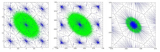
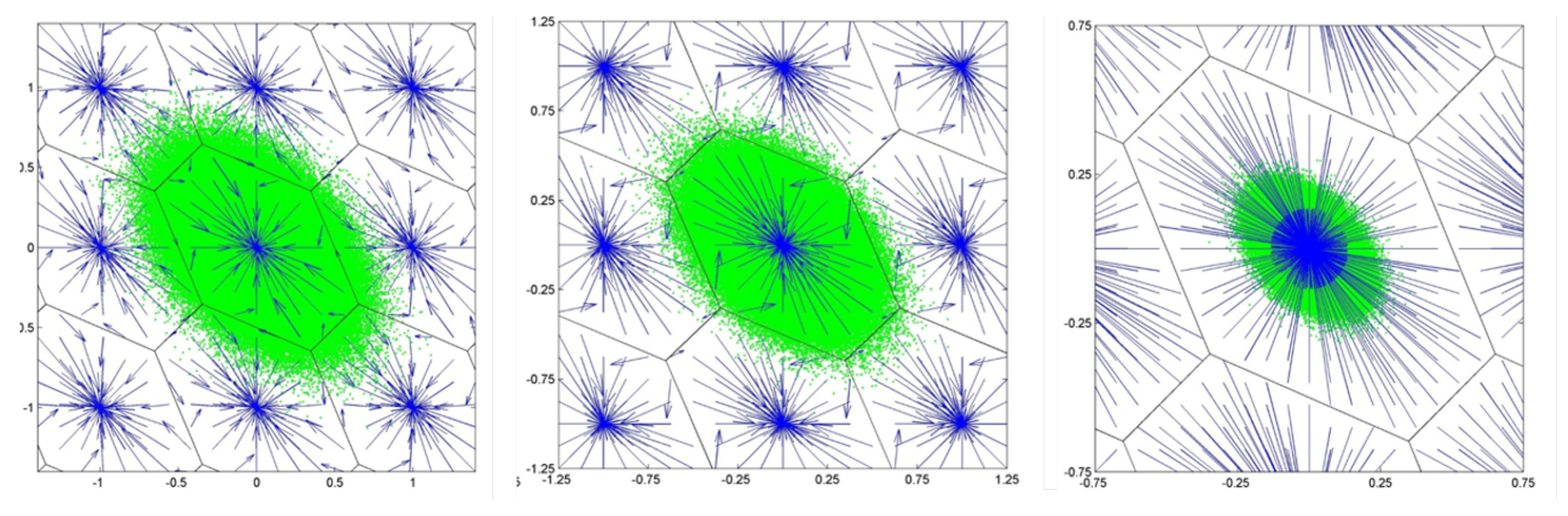
From the above BIE-expression (14), one can infer that the MSE-performance of the estimator is directly driven by the precision of the ’float’ ambiguity estimator, i.e., by $Q_{\widehat{a}\widehat{a}}$. This is illustrated in Figure 1. This figure shows three green scatterplots, which, from left to right, get smaller in relation to the hexagonal pull-in regions. The hexagons are the ILS pull-in regions ${\mathcal{P}}_z=\{x\in {\mathbb{R}}^2|\Vert x-{z\Vert }_{Q_{\widehat{a}\widehat{a}}}^2\le \Vert x-{u\Vert }_{Q_{\widehat{a}\widehat{a}}}^2,\forall u\in {\mathbb{Z}}^2\}$, while the green scatterplots are formed from Monte-Carlo simulated samples of $\widehat{a}\sim {\mathcal{N}}_2(0,Q_{\widehat{a}\widehat{a}})$, for three different levels of precision (from poor to good). The blue lines in the figure show how the BIE maps each individual float solution $\widehat{a}$ to ${\check{a}}_{\mathrm{BIE}}$. They show, from left to right, how the BIE-outcomes get closer to the centre of the pull-in region, being the ILS-solution ${\check{a}}_{\mathrm{ILS}}$, when the precision of the ambiguities improves.

Figure 1. Scatterplots (green) of $\widehat{a}\sim {\mathcal{N}}_2(0,Q_{\widehat{a}\widehat{a}})$, together with their hexagonal ILS pull-in regions ${\mathcal{P}}_z=\{x\in {\mathbb{R}}^2|\Vert x-{z\Vert }_{Q_{\widehat{a}\widehat{a}}}^2\le \Vert x-{u\Vert }_{Q_{\widehat{a}\widehat{a}}}^2,\forall u\in {\mathbb{Z}}^2\}$. The units along the axes are expressed in cycles. The scatterplots are shown, from left to right, for three different levels of precision (from poor to good). The blue lines show how samples of $\widehat{a}$ are pulled to their corresponding BIE samples ${\check{a}}_{\mathrm{BIE}}$. They show how the BIE-outcomes get closer to the ILS-solution ${\check{a}}_{\mathrm{ILS}}$, when the precision of the ambiguities improves, i.e., when, relative to the ILS pull-in regions, the scatterplots reduce in size.

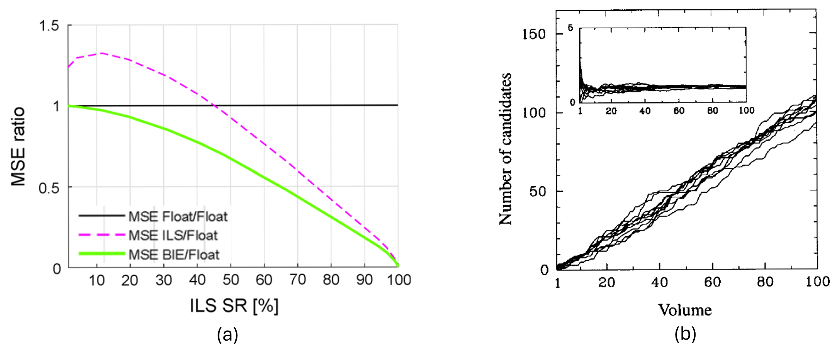
In fact, one can show that the BIE-estimator converges to the BLUE-estimator when $Q_{\widehat{a}\widehat{a}}\uparrow$, while converging to the ILS-estimator when $Q_{\widehat{a}\widehat{a}}\downarrow$. This is illustrated in Figure 2a. This dependence on $Q_{\widehat{a}\widehat{a}}$ also has numerical consequences. The more precise the float solution $\widehat{a}$ is, the more peaked the weights in (14) are and the faster they taper off for integer vectors further away from $\widehat{a}$. This implies that fewer terms in the sums of BIE are needed when $\widehat{a}$ is precise, but more when $\widehat{a}$ is not so precise. We will now show that our Fourier representation of the BIE-estimator enables us to combat the lack of numerical efficiency for this latter case. We have the following result.

Figure 2. (a) GNSS-ambiguity MSE ratios as a function of the ILS ambiguity success-rate (SR): $\mathrm{MSE}\left(\widehat{a}\right)/\mathrm{MSE}\left(\widehat{a}\right)$ (black), $\mathrm{MSE}\left({\check{a}}_{\mathrm{ILS}}\right)/\mathrm{MSE}\left(\widehat{a}\right)$ (purple), and $\mathrm{MSE}\left({\check{a}}_{\mathrm{BIE}}\right)/\mathrm{MSE}\left(\widehat{a}\right)$ (green); (b) For ten GNSS single baseline experiments, the number of integer candidate vectors contained in its ambiguity search ellipsoid ${\mathcal{E}}_{\widehat{a}}$ are shown as a function of its volume when ranging from 1 to 100. The inset shows the ratio of the number of candidates and the volume, i.e., the relative error of the volume as a predictor for the number of candidates [20,21].

Theorem 2 

(BIE in spatial and frequency domain). Let $\widehat{a}\sim N_n(a,Q_{\widehat{a}\widehat{a}})$, $a\in {\mathbb{Z}}^n$. Then the best integer equivariant estimator of a is given in spatial and frequency domains, respectively, as follows:

$$\begin{array}{ccc}{\check{a}}_{\mathrm{BIE}}\hfill & =& \widehat{a}+Q_{\widehat{a}\widehat{a}}{\partial }_{\widehat{a}}\log S\left(\widehat{a}\right),S\left(\widehat{a}\right)={\sum }_{z\in {\mathbb{Z}}^n}\exp \{-\frac{1}{2}\Vert \widehat{a}-{z\Vert }_{Q_{\widehat{a}\widehat{a}}}^2\}\hfill \\ & =& \widehat{a}+Q_{\widehat{a}\widehat{a}}{\partial }_{\widehat{a}}\log F\left(\widehat{a}\right),F\left(\widehat{a}\right)={\sum }_{z\in {\mathbb{Z}}^n}c\left(z\right)\cos \left(2\pi z^T\widehat{a}\right)\hfill \end{array}$$

(16)

with Fourier frequencies: $c\left(z\right)=\exp \{-\frac{1}{2}4{\pi }^2\Vert z{\Vert }_{Q_{\widehat{a}\widehat{a}}^{-1}}^2\}$, $z\in {\mathbb{Z}}^n$.

Proof. 

See Appendix A. □

Before we discuss the relative merit of the above two BIE-expressions, we note that the BIE ${\check{a}}_{\mathrm{BIE}}$ is obtained as a gradient correction on the BLUE $\widehat{a}$. This suggests, also with the geometry of Figure 1 in mind, that a repeated application of this mapping can be used to set up an iteration for determining the ILS solution. Indeed, it can be shown that under certain conditions the steepest ascent iteration method, $x^{(t+1)}=x^{\left(t\right)}+{\alpha }_t{Q}_{\widehat{a}\widehat{a}}{\partial }_x\log S\left(x^{\left(t\right)}\right)$, with line search ${\alpha }_t$ and initialization $x^{\left(0\right)}=\widehat{a}$, converges to ${\check{a}}_{\mathrm{ILS}}$ (instead of $S\left(x\right)$, also $F\left(x\right)$ can be used, but note that $S\left(x\right)\propto F\left(x\right)$ and not $S\left(x\right)=F\left(x\right)$). When it converges, it converges to a stationary point of $S\left(x\right)$, the stationary points of which include all integers $z\in {\mathbb{Z}}^n$. A sufficient condition for convergence to ${\check{a}}_{\mathrm{ILS}}$ is that $\widehat{a}$ should lie, just as with methods of ambiguity validation, not too close to the boundary of the pull-in region. As the analysis of this method lies outside the scope of the present contribution, we defer it to future study.

To identify the relative merit of the two BIE expressions of (16), we note that both involve infinite sums over the whole space of integers, which is, of course, computationally impractical. However, sufficient accuracy can be maintained if the infinite sums are replaced by finite sums over integers that are collected from sufficiently large search ellipsoids [1]. It is therefore here that the advantage of the two expressions shows itself. In case of the spatial representation, one collects integers that satisfy $\Vert \widehat{a}-z{\Vert }_{Q_{\widehat{a}\widehat{a}}}^2\le r^2$, while for the frequency representation, the inequality ${\Vert z\Vert }_{Q_{\widehat{a}\widehat{a}}^{-1}}^2\le {\rho }^2$ is used for the integer collection. This shows that the spatial representation has its advantage when the ambiguities are precise ($Q_{\widehat{a}\widehat{a}}$ small) and the frequency representation when the ambiguities have poor precision ($Q_{\widehat{a}\widehat{a}}^{-1}$ small). In case the ambiguity precision itself does not play a role in choosing between the two representations, one might still opt for the frequency representation, in particular when in Monte Carlo studies a large amount of $\widehat{a}$-samples are generated and one needs to choose between using $S\left(\widehat{a}\right)$ or $F\left(\widehat{a}\right)$. The fact that the frequency-coefficients $c\left(z\right)$ then need to be computed only once, while generally the repeated computation of sin and cos of a dot product is cheaper than that of an exponential of a quadratic form with dense variance matrix, would favour $F\left(\widehat{a}\right)$.

Although the above theorem clearly shows which of the two representations should be preferred in dependence on the ambiguity precision, its direct practical usage is still limited, since one will seldom be in a situation where all ambiguities have either a poor precision or a good precision. A more adjustable approach is therefore needed and one that is able to do justice to ambiguity sets that have precise and less precise ambiguities at the same time. This is made possible with the hybrid BIE form of the next section.

4. The Best Integer Equivariant Estimator in Hybrid Form

To motivate the need for the hybrid BIE form, we first show the computational complexity that the BIE formulation in the spatial domain poses when the dimension n increases. The search ellipsoid used for collecting the integer vectors is defined as follows:

$${\mathcal{E}}_{\widehat{a}}=\{z\in {\mathbb{Z}}^n\left|\right||\widehat{a}-{z\Vert }_{Q_{\widehat{a}\widehat{a}}}^2\le r^2={\chi }_{\alpha }^2(n,0)\}$$

(17)

in which $\alpha$ is a user-defined significance level (e.g., ${10}^{-6}$) of the central Chi-square distribution with n degrees of freedom. The integer candidates residing in ${\mathcal{E}}_{\widehat{a}}$ are usually collected with the state-of-the-art LAMBDA method [22]. A very good rule of thumb for the number of integer candidates, $\#z$, contained in it is the volume of the ellipsoid, which, with the volume of a unit sphere in ${\mathbb{R}}^n$ being $V_n={\displaystyle \frac{{\pi }^{n/2}}{\Gamma (n/2+1)}}$, is given as follows:

$$V_{{\mathcal{E}}_{\widehat{a}}}=V_n{\left(r\mathrm{ADOP}\right)}^n,\mathrm{with}\mathrm{ADOP}={\left|Q_{\widehat{a}\widehat{a}}\right|}^{{\displaystyle \frac{1}{2n}}}$$

(18)

Figure 2b illustrates how well the approximation $\#z\approx V_{{\mathcal{E}}_{\widehat{a}}}$ works. It shows the results of ten different, GPS single baseline experiments, thus producing ten different ambiguity variance matrices $Q_{\widehat{a}\widehat{a}}$. The actual number of candidates contained in the ambiguity search ellipsoid, $\#z$, is given as a function of the volume of the ellipsoid $V_{{\mathcal{E}}_{\widehat{a}}}$. The volume ranges from 1 to 100. The inset shows the quotient of the number of candidates and the volume, i.e., the relative error of the volume as a predictor for the number of candidates, which indeed confirms how well the approximation works. If we now use asymptotics for $V_n$ and $r^2={\chi }_{\alpha }^2(n,0)$ in (18), we obtain as a function of n the approximation $\#z\left(n\right)\approx f\left(n\right){\left(\mathrm{ADOP}\right)}^n$, in which $f\left(n\right)={\displaystyle \frac{{\left(2\pi e\right)}^{n/2}}{\sqrt{\pi n}}}$ shows, unless the $\mathrm{ADOP}$ is small enough, how the number of integer candidates explodes as a function of the dimension n. We have, for instance, $f\left(5\right)=3\times {10}^2$, $f\left(10\right)=2.6\times {10}^5$, and $f\left(15\right)=2.6\times {10}^8$.

This identified ’dimensional curse’ indeed poses a potential concern for the applicability of the spatial BIE formulation of (16) in modern-day GNSS. Instead of working with only GPS, one nowadays works predominantly with multi-GNSS [3,23,24,25,26,27,28,29], thereby integrating the observation equations of GPS, GLONASS, Galileo and BeiDou, thus quadrupling the number of ambiguities per observed frequency. This situation will be further exacerbated when mega-constellations of LEO-satellites are going to be used and integrated [30,31]. Switching from the spatial representation in (16) to its all-frequency representation is, however, not a generally valid option, as this representation will then become numerically hindered by the high precision that usually a large part of the ambiguities has. The resolution to the ’dimensional curse’ needs, therefore, to be found in a hybrid formulation of the BIE-estimator, the solution of which is given in the following theorem.

Theorem 3 

(Hybrid spatial-frequency BIE). Let $\widehat{a}={({\widehat{a}}_1^T,{\widehat{a}}_2^T)}^T$, $\check{a}={({\check{a}}_1^T,{\check{a}}_2^T)}^T$, $n=n_1+n_2$, and $Q_{11}=Q_{{\widehat{a}}_1{\widehat{a}}_1}\in {\mathbb{R}}^{n_1\times n_1}$, $Q_{22}=Q_{{\widehat{a}}_2{\widehat{a}}_2}\in {\mathbb{R}}^{n_2\times n_2}$, $Q_{21}=Q_{{\widehat{a}}_2{\widehat{a}}_1}\in {\mathbb{R}}^{n_2\times n_1}$. Then the hybrid spatial-frequency formulation of the BIE-estimator is given as follows;

$${\check{a}}_{1\mathrm{BIE}}=\sum _{z_1\in {\mathbb{Z}}^{n_1}}{\displaystyle \frac{z_1{w}_{z_1}\left({\widehat{a}}_1\right)Z_2\left({\widehat{a}}_2\left(z_1\right)\right)}{{\displaystyle \sum _{z_1\in {\mathbb{Z}}^{n_1}}}{w}_{z_1}\left({\widehat{a}}_1\right)Z_2\left({\widehat{a}}_2\left(z_1\right)\right)}}\mathrm{and}{\check{a}}_{2\mathrm{BIE}}=\sum _{z_1\in {\mathbb{Z}}^{n_1}}{\displaystyle \frac{w_{z_1}\left({\widehat{a}}_1\right)W_2\left({\widehat{a}}_2\left(z_1\right)\right)}{{\displaystyle \sum _{z_1\in {\mathbb{Z}}^{n_1}}}{w}_{z_1}\left({\widehat{a}}_1\right)Z_2\left({\widehat{a}}_2\left(z_1\right)\right)}}$$

(19)

with

$$\begin{array}{ccc}{w}_{z_1}\left({\widehat{a}}_1\right)=\exp \{-\frac{1}{2}\Vert {\widehat{a}}_1-z_1{\Vert }_{Q_{11}}^2\}\hfill & ;& Z_2\left(x\right)={\displaystyle \sum _{z_2\in {\mathbb{Z}}^{n_2}}}c\left(z_2\right)\cos \left(2\pi z_2^{T}x\right)\hfill \\ W_2\left(x\right)=Z_2\left(x\right)[x+Q_{22|1}{\partial }_x\log Z_2\left(x\right)]\hfill & ;& c\left(z_2\right)=\exp \{-\frac{1}{2}4{\pi }^2\Vert z_2{\Vert }_{Q_{22|1}^{-1}}^2\}\hfill \\ {\widehat{a}}_2\left(z_1\right)={\widehat{a}}_2-Q_{21}{Q}_{11}^{-1}({\widehat{a}}_1-z_1)\hfill & ;& Q_{22|1}=Q_{22}-Q_{21}{Q}_{11}^{-1}{Q}_{12}\hfill \end{array}$$

(20)

Proof. 

See Appendix A. □

To appreciate the above result, we note, since $W_2\left({\widehat{a}}_2\left(z_1\right)\right)/Z_2\left({\widehat{a}}_2\left(z_1\right)\right)={\widehat{a}}_2\left(z_1\right)+Q_{22|1}{\partial }_{{\widehat{a}}_2}\log Z_2\left({\widehat{a}}_2\left(z_1\right)\right)$, that the BIE of $a_2$ can be written in the $z_1$-conditional BIE of $a_2$, ${\check{a}}_{2\mathrm{BIE}}\left(z_1\right)$, as follows:

$${\check{a}}_{2\mathrm{BIE}}=\sum _{z_1\in {\mathbb{Z}}^{n_1}}{\check{a}}_{2\mathrm{BIE}}\left(z_1\right){\displaystyle \frac{w_{z_1}\left({\widehat{a}}_1\right)Z_2\left({\widehat{a}}_2\left(z_1\right)\right)}{{\displaystyle \sum _{z_1\in {\mathbb{Z}}^{n_1}}}{w}_{z_1}\left({\widehat{a}}_1\right)Z_2\left({\widehat{a}}_2\left(z_1\right)\right)}}$$

(21)

This shows how the unconditional BIE of $a_2$ can be obtained as a weighted $z_1$-sum of the conditional BIEs of $a_2$. Such computation can be done efficiently if the sum does not need too many integer candidates for $z_1$, which thus requires the ambiguities of ${\widehat{a}}_1$ to be precise, i.e., a small enough $Q_{{\widehat{a}}_1{\widehat{a}}_1}$. This efficiency, however, will be largely nullified if the $z_2$-sums, needed for the computations of the ${\widehat{a}}_2\left(z_1\right)$, require many integer candidates for $z_2$. This latter situation will occur if the spatial representation for ${\check{a}}_2\left(z_1\right)$ is used when $Q_{22|1}$ is large. Thus, for this situation, it is then best to make use of the frequency representation instead, $Z_2\left(x\right)={\sum }_{z_2\in {\mathbb{Z}}^{n_2}}c\left(z_2\right)\cos \left(2\pi z_2^{T}x\right)$, as then the frequency-coefficients $c\left(z_2\right)=\exp \{-\frac{1}{2}4{\pi }^2\left|\right|z_2{\left|\right|}_{Q_{22|1}^{-1}}^2\}$ will die out quickly when $Q_{22|1}^{-1}$ is small. The hybrid spatial-frequency formulation of the above theorem is thus suited for the case that $Q_{11}$ is small and $Q_{22|1}$ large. It will be clear that similar formulations are possible when $Q_{11}$ is large and $Q_{22|1}$ small.

The practical steps for partitioning the ambiguity vector are as follows. First one applies a LAMBDA-decorrelation (using e.g., the state-of-the-art toolbox of [22]) to the ambiguity variance matrix so as to obtain a largely decorrelated ambiguity vector $\widehat{a}$. The triangular factorization of its variance matrix, $Q_{\widehat{a}\widehat{a}}=LD{L}^T$, provides, then, through the diagonal entries of matrix D, the spectrum of sequential conditional variances ${\sigma }_{i|I}^2$, $i=1,\dots ,n$. These will usually, due to the earlier decorrelation step, already be ordered as ${\sigma }_1^2\lesssim {\sigma }_{2|1}^2\lesssim ,\dots ,\lesssim {\sigma }_{n|N}^2$. If not, then permutations are applied to achieve this ordering. To decide which part of the ambiguities should be treated spatially (i.e., $Q_{11}\in {\mathbb{R}}^{n_1\times n_1}$ small) and which part in the frequency domain (i.e., $Q_{22|1}\in {\mathbb{R}}^{(n-n_1)\times (n-n_1)}$ large), a first simple criterion is to use the ratio of the two geometric averages of the sequential conditional variances of $Q_{11}$ and $Q_{22|1}$, respectively. Hence, one would then determine $n_1$ as the minimizer of the ADOP-ratio:

$$\frac{{\mathrm{ADOP}}_1}{{\mathrm{ADOP}}_{2|1}}=\frac{\sqrt[2n_1]{|Q_{11}|}}{\sqrt[2(n-n_1)]{|Q_{22|1}|}}=\frac{\sqrt[n_1]{{\prod }_{i=1}^{n_1}{\sigma }_{i|I}}}{\sqrt[(n-n_1)]{{\prod }_{i=n_1+1}^n{\sigma }_{i|I}}}$$

(22)

A more advanced criterion would use the volumes of the respective search spaces (cf. (18)), and thus $n_1$ that minimizes the product $\#z_1\times \#z_2$, with $\#z_1\approx V_{n_1}{\left(r{\mathrm{ADOP}}_1\right)}^{n_1}$ and $\#z_2\approx V_{n-n_1}{\left(\rho {\mathrm{ADOP}}_{22|1}\right)}^{n-n_1}$ for the search spaces ${\mathcal{E}}_{\mathrm{S}}=\{z_1\in {\mathbb{Z}}^{n_1}\left|\right||{\widehat{a}}_1-z_1{\Vert }_{Q_{11}}^2\le r^2\}$ and ${\mathcal{E}}_{\mathrm{F}}=\{z_2\in {\mathbb{Z}}^{n-n_1}\left|\right||z_2{\Vert }_{Q_{22|1}^{-1}}^2\le {\rho }^2\}$, respectively.

To illustrate the workings of the theorem, consider a three-dimensional example having the following float LS-solution and variance matrix:

$$\widehat{a}=\left[\begin{array}{c}\hfill 0.49\\ \hfill 0.30\\ \hfill -0.20\end{array}\right],Q_{\widehat{a}\widehat{a}}=\left[\begin{array}{ccc}\hfill 0.01& 0.03& \hfill -0.02\\ \hfill 0.03& 0.89& \hfill 0.14\\ \hfill -0.02& 0.14& \hfill 0.64\end{array}\right]$$

(23)

Application of the LAMBDA-decorrelation [22,32], gives the transformed ambiguity vector as follows:

$$\widehat{a}≔\left[\begin{array}{c}\hfill {\widehat{a}}_1=0.49\\ \hfill {\widehat{a}}_3+2{\widehat{a}}_1=0.78\\ \hfill {\widehat{a}}_2-3{\widehat{a}}_1=-1.17\end{array}\right],Q_{\widehat{a}\widehat{a}}≔\left[\begin{array}{ccc}0.01& 0& 0\\ 0& 0.6& 0.2\\ 0& 0.2& 0.8\end{array}\right]$$

(24)

with its spectrum of sequential conditional variances, from small to large, given as ${\sigma }_1^2=0.01$, ${\sigma }_{2|1}^2=0.6$, ${\sigma }_{3|1,2}^2=0.733$. With the above criterion of choosing $n_1$ to minimize $\#z_1\times \#z_2$, the value $n_1=1$ follows. We will now use this partitioning to compare the full spatial approach to the hybrid spatial-frequency approach.

Full spatial BIE truncation: As $Q_{11}$ is small, the spatial truncation over $z_1$ is cheap. We have $w_{{\widehat{a}}_1}\left(z_1\right)=\exp \left(-\frac{1}{2}{\displaystyle \frac{{(0.49-z_1)}^2)}{0.01}}\right)$, from which it follows that only $z_1=0$ and $z_1=1$ are non-negligible, since $z_1=-1$ and $z_1=2$ already produce very small values for $w_{{\widehat{a}}_1}\left(z_1\right)$. The spatial truncation over $z_2$, however, will be expensive, since $Q_{22|1}$ is relatively large. If we consider the search ellipse $\{z_2\in {\mathbb{Z}}^2|\left|\right|{\widehat{a}}_2\left(z_1\right)-z_2{\Vert }_{Q_{22|1}}^2\le r_2^2={\chi }_{\alpha }^2(2,0)\}$, then with a significance level of $\alpha ={10}^{-8}$, we have $r_2\approx 6.07$ giving approximately 80 integer candidate points $z_2$ per $z_1$. Hence, for a full spatial truncation, already about $2\times 80=160$ integer 3D-vectors are required. In higher dimensions, this will explode rather quickly as pointed out earlier.

Hybrid spatial-frequency BIE truncation: The spatial search for $z_1$ remains unchanged, while that for $z_2$ will now be based on the frequency-based elliptical search space $\{z_2\in {\mathbb{Z}}^2\left|\exp \right\{-\frac{1}{2}4{\pi }^2\Vert z_2{\Vert }_{Q_{22|1}^{-1}}^2\}\le \beta \}$, which for $\beta ={10}^{-8}$ gives the $z_2$-set $\left\{\right(0,0),(\pm 1,0),(0,\pm 1\left)\right\}$. Hence, now the total number of required integer 3D-vectors is only $2\times 5=10$. This shows how the hybrid BIE formulation can take advantage when $Q_{11}$ is small and $Q_{22|1}$ relatively large, giving in this example a 16-times reduction in integer vector counts.

5. Summary and Conclusions

In this contribution, we introduced the concept of Fourier ambiguity resolution and demonstrated how it is rooted in the principle of IE-estimation and its periodic representation as introduced in [1]. It was shown that every IE-estimator of the mixed-integer GNSS carrier-phase model can be expressed as a periodic correction to the BLUE. Building on this structural result, a general Fourier representation of IE-estimators was established. Since the IE-class forms the most comprehensive class of estimators used in GNSS ambiguity resolution, this representation opens new perspectives for both estimation and statistical testing [8,10,28,33,34]. The framework was shown to apply not only to the general IE-class, but also to the integer class of estimators and their integer-aperture variants.

Particular attention was given to the best integer equivariant (BIE) estimator, which minimizes the mean-squared error within the IE-class. Using multivariate Fourier transform theory, spatial and frequency-domain representations of the BIE estimator were derived. Their respective merits were analyzed, and criteria were provided for selecting the preferred representation as a function of the carrier-phase ambiguity precision. We also pointed out that in the case of Monte-Carlo simulations of the BIE-estimator, the frequency-representation:

$${\check{a}}_{\mathrm{BIE}}=\widehat{a}-2\pi Q_{\widehat{a}\widehat{a}}{\displaystyle \frac{{\sum }_{z\in {\mathbb{Z}}^n}zc\left(z\right)\sin \left(2\pi z^T\widehat{a}\right)}{{\sum }_{z\in {\mathbb{Z}}^n}c\left(z\right)\cos \left(2\pi z^T\widehat{a}\right)}}$$

(25)

has the advantage that the frequency-coefficients $c\left(z\right)$ then only need to be computed once, while generally the repeated computation of sin and cos of a dot product is cheaper than that of an exponential of a quadratic form with dense variance matrix. The gradient form of the representations was also discussed, enabling implementation through steepest ascent iterations.

Finally, the spatial and frequency representations were unified in a hybrid formulation tailored to practical applications. This hybrid form accommodates ambiguity vectors with widely varying precision levels, thereby reflecting realistic GNSS conditions and enhancing practical applicability. Together, these results provide a unified spatial–frequency framework for integer equivariant estimation and establish Fourier ambiguity resolution as a natural and powerful extension of the IE paradigm.

References

- Teunissen, P.J.G. Theory of Integer Equivariant Estimation with Application to GNSS. J. Geod. 2003, 77, 402–410. [Google Scholar] [CrossRef] [Scilit]
- Leick, A.; Rapoport, L.; Tatarnikov, D. GPS Satellite Surveying, 4th ed.; John Wiley and Sons: Hoboken, NJ, USA, 2015. [Google Scholar]
- Morton, Y.; van Diggelen, F.; Spilker, J., Jr.; Parkinson, B.; Lo, S.; Gao, G. (Eds.) Position, Navigation, and Timing Technologies in the 21st Century: Integrated Satellite Navigation, Sensor Systems, and Civil Applications; Wiley: Hoboken, NJ, USA, 2020. [Google Scholar]
- Teunissen, P.J.G. Best integer equivariant estimation for elliptically contoured distributions. J. Geod. 2020, 94, 82. [Google Scholar] [CrossRef] [Scilit]
- Arnold, S.F. Mathmatical Statistics; Prentice Hall: Englewood Cliffs, NJ, USA, 1990. [Google Scholar]
- Champeney, D.C. A Handbook of Fourier Theorems; Cambridge University Press: Cambridge, UK, 1987. [Google Scholar]
- Osborne, A.R. Nonlinear Ocean Waves and the Inverse Scattering Transform; Volume 97 of International Geophysics Series; Academic Press: Cambridge, MA, USA, 2010. [Google Scholar]
- Brack, A.; Gunther, C. Generalized integer aperture estimation for partial GNSS ambiguity fixing. J. Geod. 2014, 88, 479–490. [Google Scholar] [CrossRef] [Scilit]
- Brack, A. On reliable data-driven partial GNSS ambiguity resolution. GPS Solut. 2015, 19, 411–422. [Google Scholar] [CrossRef] [Scilit]
- Teunissen, P.J.G. Ambiguity-Resolved Model Tests for Carrier-Phase GNSS. Appl. Sci. 2025, 15, 3531. [Google Scholar] [CrossRef] [Scilit]
- Duong, V.; Harima, K.; Choy, S.; Rizos, C. GNSS best integer equivariant estimation using multivariant t-distribution: A case study for precise point positioning. J. Geod. 2021, 95, 10. [Google Scholar] [CrossRef] [Scilit]
- Odolinski, R.; Teunissen, P.J.G. Best integer equivariant position estimation for multi-GNSS RTK: A multivariate normal and t-distributed performance comparison. J. Geod. 2022, 96, 3. [Google Scholar] [CrossRef] [Scilit]
- Ma, L.; Lou, L.; Lu, L.; Liu, W.; Zhu, F. GNSS best integer equivariant estimation combining with integer least squares estimation: An integrated ambiguity resolution method with optimal integer aperture test. GPS Solut. 2022, 26, 100. [Google Scholar] [CrossRef] [Scilit]
- Brack, A.; Männel, B.; Schuh, H. Two-epoch centimeter-level PPP-RTK without external atmospheric corrections using best integer-equivariant estimation. GPS Solutions 2023, 27, 12. [Google Scholar] [CrossRef] [Scilit]
- Brack, A.; Männel, B.; Schuh, H. Almost-Instantaneous PPP-RTK Without Atmospheric Corrections. In Gravity, Positioning and Reference Frames. REFAG 2022; International Association of Geodesy Symposia; Freymueller, J.T., Sánchez, L., Eds.; Springer Nature: Cham, Switzerland, 2023; Volume 156. [Google Scholar]
- Liu, Y.; Liu, W.; Zhang, X.; Liang, Y.; Tao, X.; Ma, L. An improved GNSS ambiguity best integer equivariant estimation method with Laplacian distribution for urban low-cost RTK positioning. Satell. Navig. 2024, 5, 12. [Google Scholar] [CrossRef] [Scilit]
- Miao, W.; Li, B.; Gao, Y.; Chen, G. Vectorial integer bootstrapping of best integer equivariant estimation (VIB-BIE) for efficient and reliable GNSS ambiguity resolution. J. Geod. 2024, 98, 30. [Google Scholar] [CrossRef] [Scilit]
- Yang, Y.; Zhou, F.; Song, S. Improving precise point positioning (PPP) performance with best integer equivariant (BIE) estimator. GPS Solut. 2024, 28, 50. [Google Scholar] [CrossRef] [Scilit]
- Wu, Z.; Bian, S. Applications of GNSS BIE-ECDs theory to the least-squares estimator of the integer ambiguity. J. Geod. 2026, 100, 8. [Google Scholar] [CrossRef] [Scilit]
- Teunissen, P.J.G.; de Jonge, P.J.; Tiberius, C.C.J.M. The volume of the GPS ambiguity search space and its relevance for integer ambiguity resolution. In Proceedings of the 9th International Technical Meeting of the Satellite Division of The Institute of Navigation (ION GPS 1996), Kansas City, MO, USA, 17–20 September 1996. [Google Scholar]
- Odolinski, R.; Teunissen, P.J.G. Best integer equivariant estimation: Performance analysis using real data collected by low-cost, single- and dual-frequency, multi-GNSS receivers for short- to long-baseline RTK positioning. J. Geod. 2020, 94, 91. [Google Scholar] [CrossRef] [Scilit]
- Massarweh, L.; Verhagen, S.; Teunissen, P.J.G. New LAMBDA toolbox for mixed-integer models: Estimation and evaluation. GPS Solut. 2025, 29, 14. [Google Scholar] [CrossRef] [Scilit]
- Strang, G.; Borre, K. Linear Algebra, Geodesy, and GPS; Wellesley-Cambridge Press: Wellesley, MA, USA, 1997. [Google Scholar]
- Hofmann-Wellenhof, B.; Lichtenegger, H.; Wasle, E. (Eds.) GNSS: Global Navigation Satellite Systems. GPS, GLONASS, Galileo and more; Springer: New York, NY, USA, 2008; ISBN 978-3-211-73012-6. [Google Scholar]
- Khodabandeh, A.; Zaminpardaz, S.; Nadarajah, N. A study on multi-GNSS phase-only positioning. Meas. Sci. Technol. 2021, 32, 095005. [Google Scholar] [CrossRef] [Scilit]
- Paziewski, J.; Fortunato, M.; Mazzoni, A.; Odolinski, R. An analysis of multi-GNSS observations tracked by recent Android smartphones and smartphone-only relative positioning results. Measurement 2021, 175, 109162. [Google Scholar] [CrossRef] [Scilit]
- Yong, C.Z.; Odolinski, R.; Zaminpardaz, S.; Moore, M.; Rubinov, E.; Er, J.; Denham, M. Instantaneous, Dual-Frequency, Multi-GNSS Precise RTK Positioning Using Google Pixel 4 and Samsung Galaxy S20 Smartphones for Zero and Short Baselines. Sensors 2021, 21, 8318. [Google Scholar] [CrossRef] [Scilit]
- Khodabandeh, A. Bias-bounded estimation of ambiguity: A method for radio interferometric positioning. IEEE Trans. Signal Process. 2022, 70, 3042–3057. [Google Scholar] [CrossRef] [Scilit]
- Mohamadi, A.; Nahavandchi, H.; Khodabandeh, A. Phase-Only positioning in urban environments: Assessing its potential formass-market GNSS receivers. J. Spat. Sci. 2025, 70, 557–569. [Google Scholar] [CrossRef] [Scilit]
- Khalife, J.; Kassas, Z.Z.M. Performance-driven design of carrier phase differential navigation frameworks with megaconstellation LEO satellites. IEEE Trans. Aerosp. Electron. Syst. 2023, 59, 2947–2966. [Google Scholar] [CrossRef] [Scilit]
- Stock, W.; Schwarz, R.T.; Hofmann, C.A.; Knopp, A. Survey On Opportunistic PNT With Signals From LEO Communication Satellites. IEEE Commun. Surv. Tutor. 2024, 27, 77–107. [Google Scholar] [CrossRef] [Scilit]
- Teunissen, P.J.G. The least squares ambiguity decorrelation adjustment: A method for fast GPS integer estimation. J. Geod. 1995, 70, 65–82. [Google Scholar] [CrossRef] [Scilit]
- Brack, A.; Henkel, P.; Gunther, C. Sequential Best Integer-Equivariant Estimation for GNSS. Navigation 2014, 61, 149–158. [Google Scholar] [CrossRef] [Scilit]
- Brack, A. Vectorial Sequential Best Integer-Equivariant Estimation for GNSS. In Navigating the Geodetic Landscape: A Tribute to 45 Years of Excellence, Chapter 11; Khodabandeh, A., Verhagen, S., Eds.; Springer: Cham, Switzerland, 2025. [Google Scholar]
- Stark, H.; Woods, J.W. Probability, Random Processes, and Estimation Theory for Engineers; Prentice Hall: Englewood Cliffs, NJ, USA, 1986. [Google Scholar]
Disclaimer/Publisher’s Note: The statements, opinions and data contained in all publications are solely those of the individual author(s) and contributor(s) and not of MDPI and/or the editor(s). MDPI and/or the editor(s) disclaim responsibility for any injury to people or property resulting from any ideas, methods, instructions or products referred to in the content. |
© 2026 by the author. Licensee MDPI, Basel, Switzerland. This article is an open access article distributed under the terms and conditions of the Creative Commons Attribution (CC BY) license.