Closed-Loop System Identification and Gain Scheduled Control of Piston Engine–Dynamometer System with Disturbance Observer

Abstract

Piston engine system identification models are crucial for autonomous and control-oriented applications. However, piston engines exhibit relatively unstable behavior, which may lead to overspeed during open-loop operation. In this study, system identification of a piston engine is investigated on a piston engine–dynamometer test bench. The identification process is carried out under closed-loop conditions to ensure safe and reliable operation. Known system parameters are utilized to transform the closed-loop system into an equivalent open-loop representation. Three system identification models—a State-Space model, a nonlinear ARX model, and a Hammerstein–Wiener model—are employed and comparatively evaluated. The identified models are validated based on their closed-loop responses. Subsequently, a gain scheduled cruise controller is designed using the identified model and implemented on an engine dynamic model. Finally, a disturbance observer is integrated into the cruise controller to enhance disturbance rejection performance. The disturbance observer is developed based on the identified system model.

1. Introduction

Engine model is a crucial process for engine controller design because it provides effective testing and simulation possibilities [1]. Numerous modeling methods are deployed into piston engines for closed-loop control [2]. Early modeling methods started with modeling subsystems such as throttle body, manifold, crankshaft, and injection system with physical laws [3]. Then, experimental data is used to feed the mathematical model of piston engines [4]. The Mean Value Engine Model (MVEM) is proposed to adjust mathematical model coefficients by mean value error criteria in experimental datasets [1]. The mean value model is widely used to present engine model, and higher accuracy is achieved by adding more subsystem into model and increasing model complexity [1]. Although the MVEM is widely used and has high accuracy, it requires aerodynamic and thermodynamic knowledge; it also requires piston engine mechanical part specification. Thus, system identification methods are employed to create piston engine dynamic models [5]. In addition to classical system identification methods, neural-network-based approaches, such as recurrent neural networks (RNNs), deep neural networks (DNNs), and more recently transformer-based architectures, have been applied to engine modeling due to their strong capability in capturing nonlinear and time-dependent system dynamics [6,7,8,9]. However, these approaches typically require large datasets, and their use in control-oriented applications remains limited due to challenges in interpretability, stability analysis, and controller design [10,11,12]. Therefore, in this study classical identification models such as State-Space, nonlinear ARX and Hammerstein–Wiener are employed. System identification on a piston engine is a challenging process; it requires load torque which is provided by a dynamometer. In case of no load conditions, engine speed can go overspeed. System identification on the dynamometer–engine system is being investigated by some researchers. In ref. [13], the engine is represented as a first-order transfer function with time delay and assumes the dynamometer as a first-order transfer function; then, system identification methods are applied on frequency domain and design controller to keep the system at the desired speed and torque curve. In ref. [13], system identification is performed separately for the engine and the dynamometer. In ref. [14], the engine is modeled as a first-order system with time delay. System identification is performed separately for the engine–dynamometer model, and a controller is designed to maintain the desired speed and torque profile. In ref. [15], parameter estimation is performed for the dynamometer–engine system, and the study focuses on controller design following the system identification process. In previous studies, the system identification processes are applied on system while the system is driven with open-loop operation. In this work, piston engine system identification is applied while the test bench is operated in closed-loop mode. Closed-loop system identification provides safe, time-efficient and accurate system identification on piston engines. In closed-loop operation, the electrical DC motor dynamometer regulates test bench speed at the desired value and engine torque is adjusted by the engine’s throttle. From a control perspective, the engine–dynamometer system can be characterized as a nonlinear system affected by disturbances and parameter variations, where maintaining the desired operating condition is critical. Nonlinear control strategies and model-based control approaches have been widely studied to handle such systems, particularly in the presence of external disturbances [16,17]. In this context, gain scheduling is employed to handle system nonlinearities by adapting controller parameters across operating conditions. Furthermore, disturbance observer (DOB)-based methods are utilized to estimate and compensate unknown disturbances affecting engine torque. Therefore, the proposed approach combines gain scheduling and disturbance observer design to achieve effective disturbance compensation.

2. Piston Engine–Dynamometer System

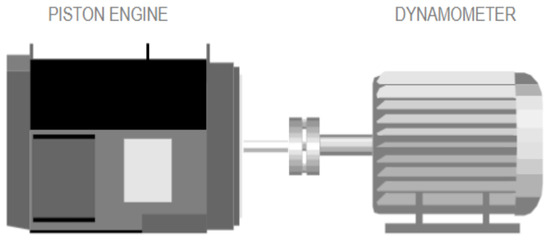
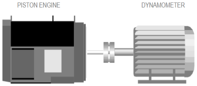
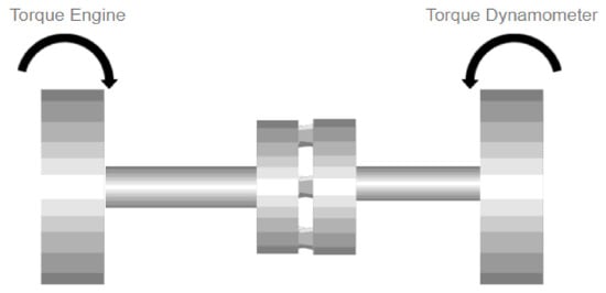
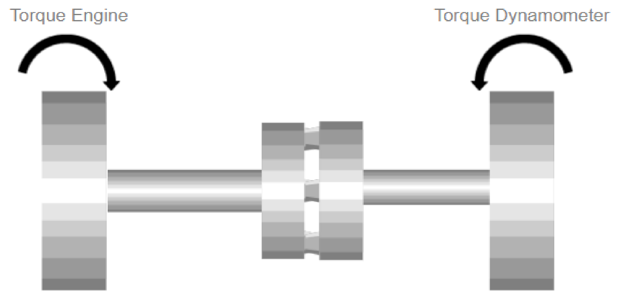
In the industry, piston engine performance tests are carried out via dynamometer setups. These tests aim at extracting piston engine torque-speed, temperature and fuel consumption characteristics. The dynamometer is connected to piston engine shaft as seen in Figure 1. Dynamometer is an essential part of the test bench because the piston engine is a relatively unstable system. This means that the engine can go overspeed at no load condition. The dynamometer provides brake torque for the piston engine, thus regulating piston engine speed and preventing overspeed cases. Dynamometers may have different types such as hydraulic, electric motors, and eddy current-actuated ones [18].

Figure 1. Piston engine–dynamometer system representation.

In this work, the dynamometer system was selected as the DC motor type, which has adequate control performance [18].

In closed-loop operation, the dynamometer controls system speed by adjusting brake torque. Since the dynamometer is connected to the engine shaft, the piston engine and dynamometer have the same speed.

2.1. Piston Engine Model

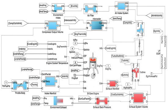
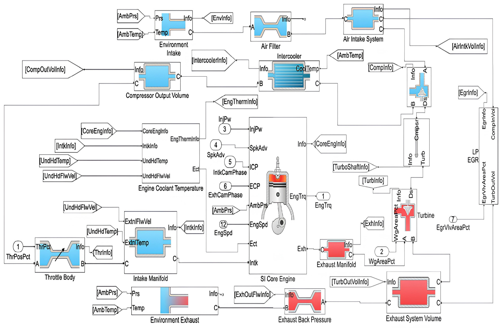
The engine model is deployed in the Simulink environment. A 1.5 L Spark-Ignited turbocharged engine model is used as the engine dynamic model, as seen in Figure 2 [19]. The model includes air mass flow dynamic components such as environmental intake, air filter, air intake system, compressor, throttle body, intake manifold and turbocharger. The model is based on air flow into a piston cylinder. The air flow is expressed as engine parameters, engine speed and throttle angle. Engine torque is derived from engine speed–air mass look-up tables. The detailed expression for the engine model is explained in the [19].

Figure 2. Engine dynamic model at Simulink environment.

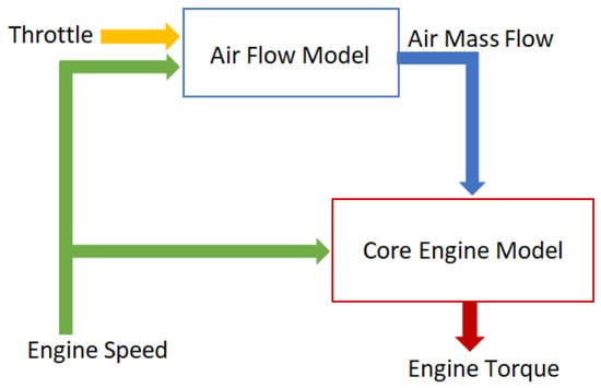
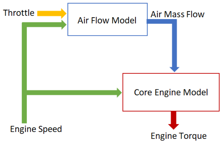
A simplified representation of the engine model structure is shown in Figure 3.

Figure 3. Engine model diagram.

In an engine model, the engine torque $T_{eng}$ is a function of engine speed $en{g}_{speed}$, throttle angle $throttl{e}_{angle}$ and engine parameters $en{g}_{param}$ as expressed in Equation (1).

$$T_{eng}=f\left(en{g}_{param},en{g}_{speed},throttl{e}_{angle}\right)$$

(1)

$f$ function includes differential functions, nonlinearities and look-up tables.

The main symbols and variables used throughout this study are summarized in Table 1 for clarity and ease of reference.

Table 1. Summary of notations.

Symbol	Description
$T_{eng}$	Engine torque
$T_{dyno}$	Dynamometer torque
$Loa{d}_{torque}$	External load torque
$G_{idsm}$	Identified minimum phase engine model
$G_{dyno}$	Dynamometer dynamics
$G_{sys}$	Transmission dynamics
$G_{filter}$	Low pass filter used to obtain implementable system
$thr$	Throttle input
$Th{r}_{dist}$	Throttle compensation signal from disturbance observer
$spd$	System speed
$ref$	Speed reference
$err$	Speed error
$PI$	PI controller
$V\left(t\right)$	Motor voltage
$V_{controller}\left(t\right)$	Controller output voltage
$V_{bias}\left(t\right)$	Bias voltage
$i\left(t\right)$	Motor current
$L$	Motor inductance
$R$	Motor resistance

2.2. Dynamometer Model

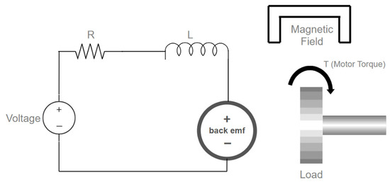
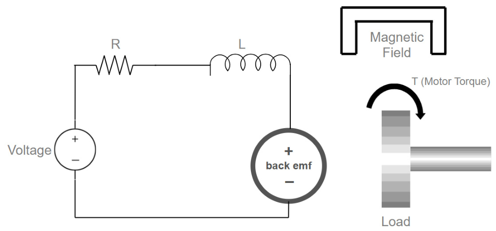
In this work, a DC motor type dynamometer is deployed and modeled with an equivalent circuit model as in shown in Figure 4.

$$L·{\displaystyle \frac{di\left(t\right)}{dt}}+R·i\left(t\right)=V\left(t\right)-emf·moto{r}_{speed}$$

(2)

$$T_{motor}=K_t · i\left(t\right)$$

(3)

$$L=motor inductance R=motor resistance$$

$$i \left(t\right)=motor current V\left(t\right)=motor voltage$$

$$moto{r}_{speed}=motor speed emf=back emf constant$$

$$K_t=torque constant T_{motor}=torque of motor$$

Figure 4. Dc motor model.

2.3. Transmission Model

The piston engine and the dynamometer are connected by a shaft, thus their speeds are the same. The engine intends to accelerate the system, and the dynamometer intends to decelerate the system. The transmission system illustrated in Figure 5 and its dynamics are expressed in Equation (4).

$$J_{system}\dot{\omega }=T_{engine}-T_{dyno}-B_{system}\omega$$

(4)

$$J_{system}=Inertia of system T_{dyno}=Dynamometer Torque$$

$$B_{system}=Friction coefficient T_{engine}=Engine Torque$$

$$\omega =System angular speed \dot{\omega }=System angular acceleration$$

Figure 5. Transmission system representation.

3. Closed-Loop System Identification

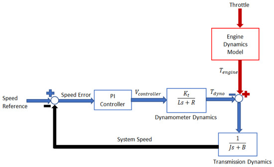
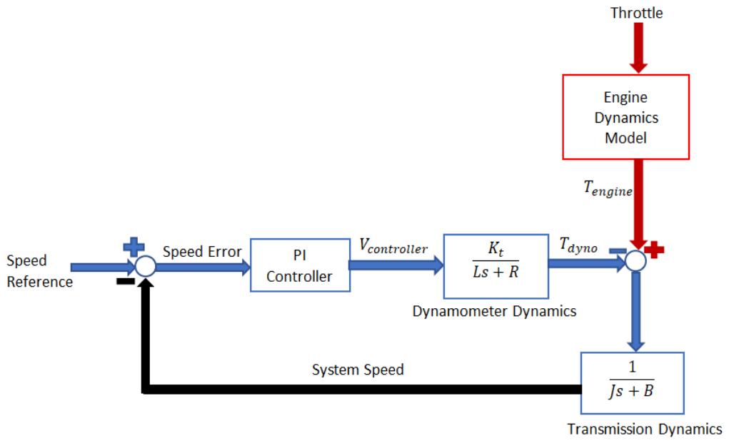
In this work, the dynamometer controller is selected as PI for its linearity properties. The system speed is kept constant by the dynamometer controller during the dynamometer test operation by adjusting dynamometer torque $T_{dyno}$. Thus, $moto{r}_{speed}$ in Equation (2) is assumed to be a constant value. Bias voltage is added to controller response to eliminate the back emf effect on motor dynamics as depicted in Equation (2).

$$V\left(t\right)=V_{controller}\left(t\right)+V_{bias}\left(t\right)$$

(5)

$$V_{bias}\left(t\right)=emf·moto{r}_{speed}\left(t\right)$$

(6)

$$V\left(t\right)=Motor Voltage V_{bias}\left(t\right)=Bias Voltage$$

$$moto{r}_{speed}=Dynamometer System Speed$$

$$V_{controller}\left(t\right)=Controller Response Voltage emf=back emf constant$$

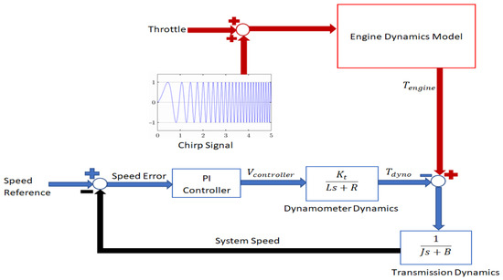
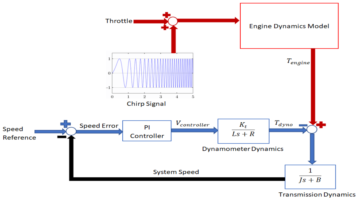
The closed-loop system diagram is shown in Figure 6.

Figure 6. Dynamometer system closed-loop diagram.

The controller, dynamometer dynamics and transmission dynamics are the known systems, but the engine model is an unknown blackbox system. In the literature, researchers have focused on closed-loop system identification [20,21,22,23]. In ref. [20], system identification is performed on a closed-loop system by converting it into an open-loop system. In ref. [21], a method for converting a closed-loop system into an open-loop system is also suggested. In this work, the closed-loop system is transformed into an equivalent open-loop system, where the input is speed error $err$ and the output is engine torque $T_{eng}$.

$$T_{eng}\left(t\right)=\mathrm{e}\mathrm{n}\mathrm{g}\mathrm{i}\mathrm{n}\mathrm{e} \mathrm{t}\mathrm{o}\mathrm{r}\mathrm{q}\mathrm{u}\mathrm{e}$$

$$T_{dyno}\left(t\right)=\mathrm{d}\mathrm{y}\mathrm{n}\mathrm{a}\mathrm{m}\mathrm{o}\mathrm{m}\mathrm{e}\mathrm{t}\mathrm{e}\mathrm{r} \mathrm{t}\mathrm{o}\mathrm{r}\mathrm{q}\mathrm{u}\mathrm{e}$$

$$thr\left(t\right)=\mathrm{t}\mathrm{h}\mathrm{r}\mathrm{o}\mathrm{t}\mathrm{t}\mathrm{l}\mathrm{e} \mathrm{i}\mathrm{n}\mathrm{p}\mathrm{u}\mathrm{t}$$

$$spd\left(t\right)=\mathrm{s}\mathrm{y}\mathrm{s}\mathrm{t}\mathrm{e}\mathrm{m} \mathrm{s}\mathrm{p}\mathrm{e}\mathrm{e}\mathrm{d}$$

$$ref\left(t\right)=\mathrm{s}\mathrm{p}\mathrm{e}\mathrm{e}\mathrm{d} \mathrm{r}\mathrm{e}\mathrm{f}\mathrm{e}\mathrm{r}\mathrm{e}\mathrm{n}\mathrm{c}\mathrm{e}$$

$$err\left(t\right)=ref\left(t\right)-spd\left(t\right)$$

$$G_{eng}=\mathrm{e}\mathrm{n}\mathrm{g}\mathrm{i}\mathrm{n}\mathrm{e} \mathrm{d}\mathrm{y}\mathrm{n}\mathrm{a}\mathrm{m}\mathrm{i}\mathrm{c}\mathrm{s}$$

$$G_{dyno}=\mathrm{d}\mathrm{y}\mathrm{n}\mathrm{a}\mathrm{m}\mathrm{o}\mathrm{m}\mathrm{e}\mathrm{t}\mathrm{e}\mathrm{r} \mathrm{d}\mathrm{y}\mathrm{n}\mathrm{a}\mathrm{m}\mathrm{i}\mathrm{c}\mathrm{s}$$

$$G_{sys}=\mathrm{t}\mathrm{r}\mathrm{a}\mathrm{n}\mathrm{s}\mathrm{m}\mathrm{i}\mathrm{s}\mathrm{s}\mathrm{i}\mathrm{o}\mathrm{n} \mathrm{d}\mathrm{y}\mathrm{n}\mathrm{a}\mathrm{m}\mathrm{i}\mathrm{c}\mathrm{s}$$

$$PI=\mathrm{P}\mathrm{r}\mathrm{o}\mathrm{p}\mathrm{o}\mathrm{r}\mathrm{t}\mathrm{i}\mathrm{n}\mathrm{a}\mathrm{l}-\mathrm{i}\mathrm{n}\mathrm{t}\mathrm{e}\mathrm{g}\mathrm{r}\mathrm{a}\mathrm{l} \mathrm{c}\mathrm{o}\mathrm{n}\mathrm{t}\mathrm{r}\mathrm{o}\mathrm{l}\mathrm{l}\mathrm{e}\mathrm{r}$$

$$T_{eng}=thr \ast G_{eng}$$

(7)

$$T_{dyno}=err \ast PI \ast G_{dyno}$$

(8)

$${(T}_{eng}-T_{dyno}) \ast G_{sys }=spd$$

(9)

$$ref-{(T}_{eng}-T_{dyno}) \ast G_{sys }=err$$

(10)

$$ref-\left(thr \ast G_{eng}-err \ast PI \ast G_{dyno}\right) \ast G_{sys }=err$$

(11)

$$ref-\left(thr \ast G_{eng} \ast G_{sys}\right)=err\left(1+PI \ast G_{dyno} \ast G_{sys}\right)$$

(12)

$$err={\displaystyle \frac{ref-thr \ast G_{eng} \ast G_{sys}}{(1+PI \ast G_{dyno} \ast G_{sys})}}$$

(13)

$$err \ast \left(1+PI \ast G_{dyno} \ast G_{sys}\right)=ref-thr \ast G_{eng} \ast G_{sys }$$

(14)

$$thr \ast G_{eng} \ast G_{sys}=ref-err \ast \left(1+PI \ast G_{dyno} \ast G_{sys}\right)$$

(15)

$$T_{eng}={\displaystyle \frac{ref-err \ast \left(1+PI \ast G_{dyno} \ast G_{sys}\right)}{G_{sys}}}$$

(16)

Note that in Equation (16), ${\displaystyle \frac{1}{G_{sys}}}$ term is a non-causal system. It cannot be modeled mathematically. Thus,$G_{Filter}$ is deployed. $G_{Filter}$ is a low pass filter and makes ${\displaystyle \frac{G_{sys}}{G_{Filter}}}$ implementable. The same concept is used in the disturbance observer design as the Q(s) filter [24].

$$T_{eng} \ast G_{Filter}=\left(ref-err \ast \left(1+PI \ast G_{dyno} \ast G_{sys}\right)\right) \ast \left({\displaystyle \frac{G_{Filter}}{G_{sys}}}\right)$$

(17)

$G_{Filter}$’s cut-off frequency should be chosen to be too high; therefore, it does not affect system identification performance. Engine torque is derived from the measured values and system parameters as expressed in Equation (17). Speed error $err$ is a measured value and system speed reference $ref$, dynamometer controller PI, dynamometer dynamic $G_{dyno}$, transmission dynamic $G_{sys}$, and low pass filter $G_{Filter}$ are known parameters.

In this work, the chirp signal, which is commonly used in the identification process, is injected into throttle command. Its formula is expressed in Equation (18) [23].

$$u\left(t\right)=Acos(w_{1}t+{(w}_2-w_1)\left({\displaystyle \frac{t^2}{2N}}\right))$$

(18)

$$w_1= initial frequency , w_2=final frequency$$

$$t=time index, N=time period 0<t<N$$

The dynamometer controller tries to keep the system at constant reference speed; then, a chirp signal is added to the throttle command. The identification process is shown in Figure 7. Engine torque $T_{eng},$ is obtained from Equation (17).

Figure 7. System identification diagram.

In the simulation, the LEM-200D135RAGS motor was chosen as a dynamometer. Its parameters are shown in Table 2 [25].

Table 2. LEM-200D135RAGS parameters.

Name	Parameter	Value	Unit
Torque Constant	$K_t$	0.21	Nm/A
Back Emf Constant	emf	0.239	V/(rad/s)
Electrical Resistance	$R$	16.95	mΩ
Inductance	L	16	uH

Transmission system parameters are taken from [15], as shown in Table 3.

Table 3. Transmission system parameters.

Name	Parameter	Value	Unit
System Inertia	$J_{system}$	0.155	Kg·m2
Friction Coefficient	${ B}_{system}$	0.089	Nm·(s/rad)

The simulation engine model is deployed as a 1.5 L Spark-Ignited turbocharged engine. The dynamometer controller is iteratively tuned. Note that this work does not focus on dynamometer controller design, thus the dynamometer controller is tuned iteratively. PI values are indicated in Table 4.

Table 4. PI controller parameters.

Name	Parameter	Value	Unit
Proportional Term	$P$	1.05
Integration Term	$I$	0.95
Reference speed	ref	2000	rpm

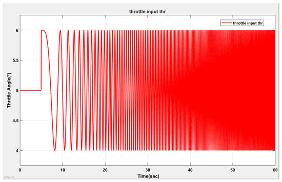
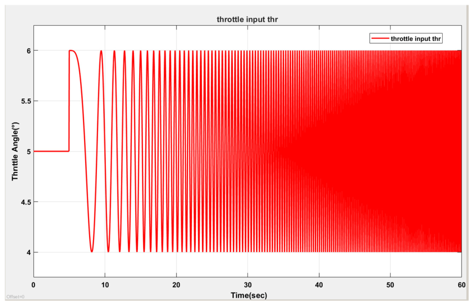
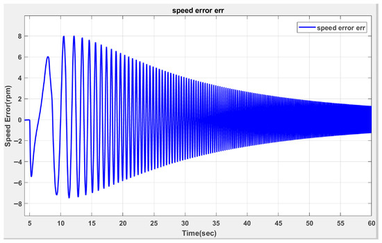
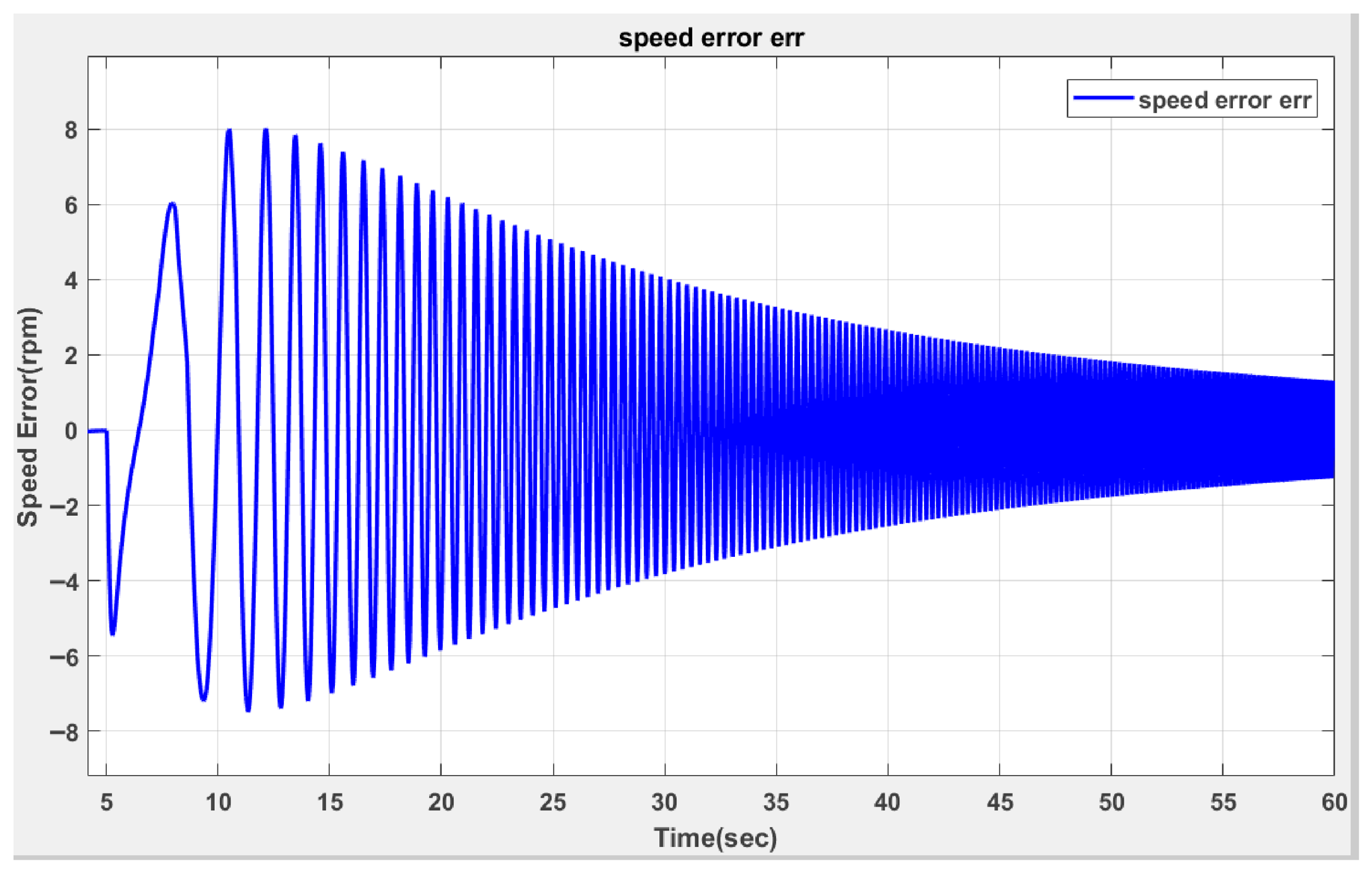
After the closed-loop system reaches steady state, chirp signal is injected into the throttle input and speed error is recorded, as shown in Figure 8 and Figure 9.

Figure 8. Throttle position in the system identification process.

Figure 9. Speed error in the system identification process.

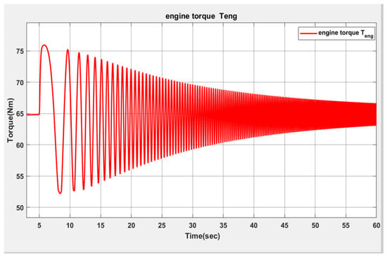
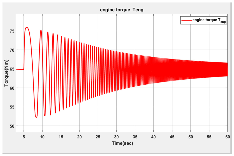
Motor torque,$T_{eng}$, is derived from Equation (17) as shown in Figure 10.

Figure 10. Motor torque, ${\mathit{T}}_{\mathit{e}\mathit{n}\mathit{g}}$, in system identification process.

4. System Identification Methods

Three system identification methods—the State-Space model, nonlinear ARX model and Hammerstein–Wiener model—are deployed. Three methods are commonly used in the identification of piston engine dynamics [26,27,28].

4.1. State-Space Model

The State-Space model is depicted in Equation (19). $A,B,C,D$ are State-Space matrices, $x\left(t\right)$ is the state vector, $u\left(t\right)$ is the system input, $y\left(t\right)$ is the system output, $d\left(t\right)$ is the disturbance and $K$ is disturbance distribution matrix.

$$\dot{x}\left(t\right)=Ax\left(t\right)+Bu\left(t\right)+Kd\left(t\right)$$

(19)

$$y\left(t\right)=Cx\left(t\right)+Du\left(t\right)+d\left(t\right)$$

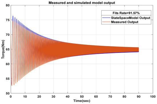
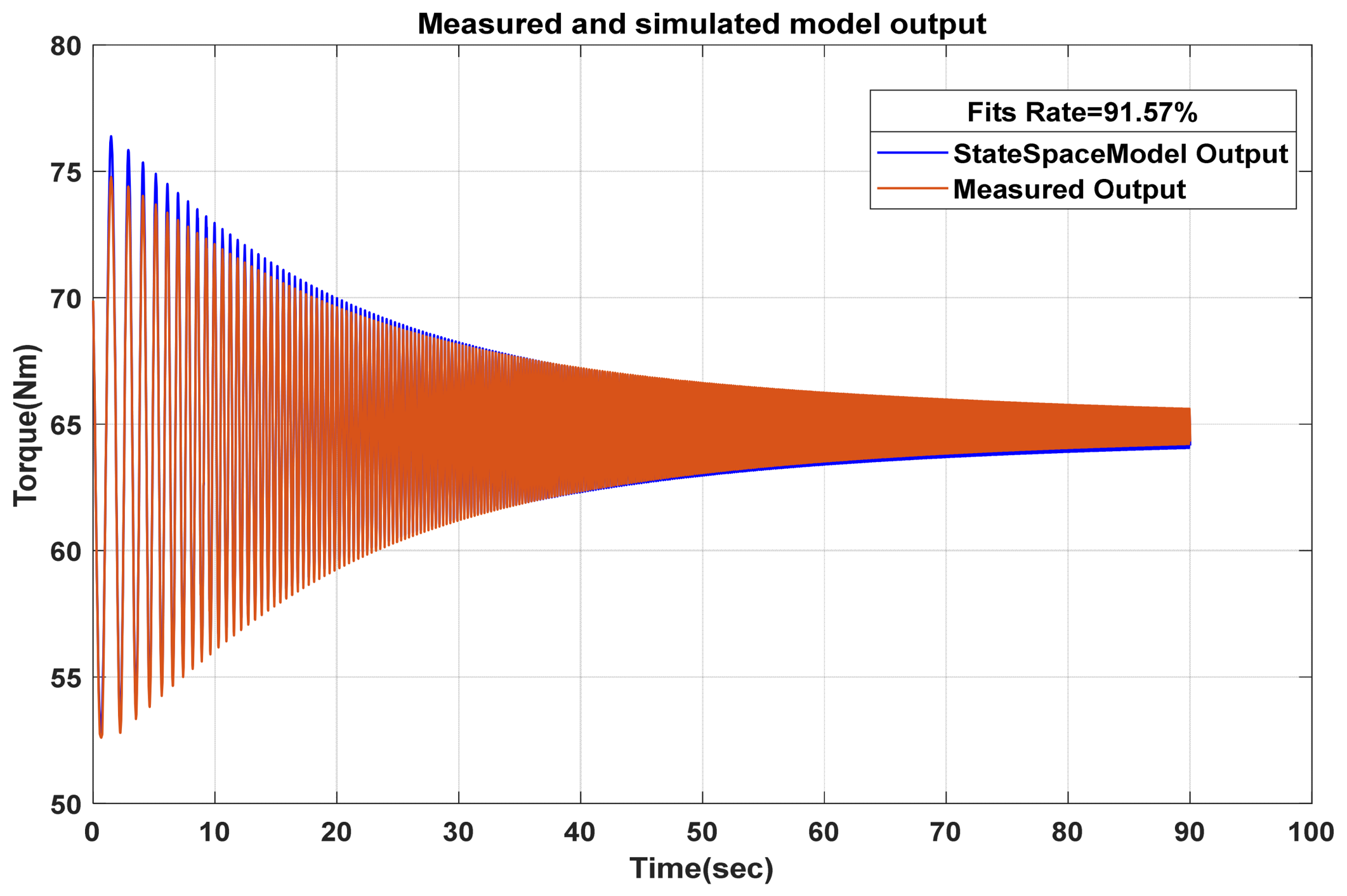
The Subspace State-Space system identification (N4SID) method uses numerical techniques for the identification process. This method is commonly used for State-Space model identification [29]. The State-Space System is chosen as a second order and the model reaches 91.57% simulation fits, as seen in Figure 11.

Figure 11. State-Space model system identification result.

4.2. Nonlinear ARX Model

The nonlinear ARX Model uses past input and output states and the input’s current states to compute the current output states, as seen in Equation (20) [30].

$$y\left(t\right)=F(y\left(t-1\right),y\left(t-2\right), \dots ,y\left(t-a\right),u\left(t\right),u\left(t-1\right), u(t-2),...,u\left(t-b\right) )$$

(20)

$$F=\mathrm{o}\mathrm{u}\mathrm{t}\mathrm{p}\mathrm{u}\mathrm{t} \mathrm{m}\mathrm{a}\mathrm{p}\mathrm{p}\mathrm{i}\mathrm{n} \mathrm{f}\mathrm{u}\mathrm{n}\mathrm{c}\mathrm{t}\mathrm{i}\mathrm{o}\mathrm{n}$$

$$a=\mathrm{n}\mathrm{u}\mathrm{m}\mathrm{b}\mathrm{e}\mathrm{r} \mathrm{o}\mathrm{f} \mathrm{o}\mathrm{u}\mathrm{t}\mathrm{p}\mathrm{u}\mathrm{t} \mathrm{p}\mathrm{a}\mathrm{s}\mathrm{t} \mathrm{t}\mathrm{e}\mathrm{r}\mathrm{m}$$

$$b=\mathrm{n}\mathrm{u}\mathrm{m}\mathrm{b}\mathrm{e}\mathrm{r} \mathrm{o}\mathrm{f} \mathrm{i}\mathrm{n}\mathrm{p}\mathrm{u}\mathrm{t} \mathrm{p}\mathrm{a}\mathrm{s}\mathrm{t} \mathrm{t}\mathrm{e}\mathrm{r}\mathrm{m}$$

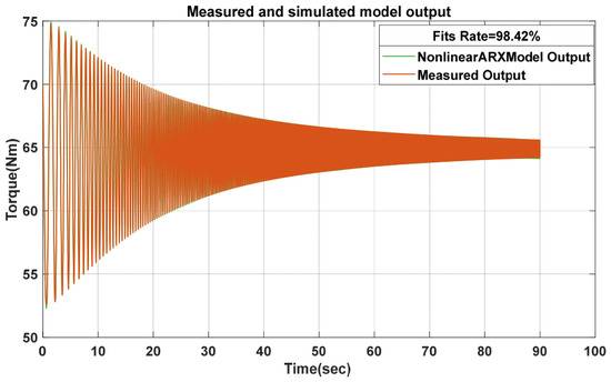
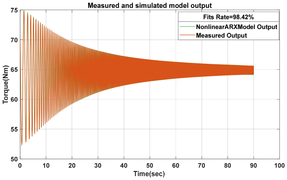
In the nonlinear ARX model, nonlinearity is configured as a Wavelet Network. The a term is selected as 2 and the b term is selected as 2. As seen in Figure 12, the nonlinear ARX model reached 98.42% fitting rate.

Figure 12. Nonlinear ARX model system identification result.

4.3. Hammerstein–Wiener Model

The Hammerstein–Wiener model includes linear and nonlinear blocks to describe systems, as seen in Figure 13. A linear block describes system dynamics. Nonlinear blocks represent nonlinear effects such as saturation or dead zone [31].

Figure 13. Hammerstein–Wiener model representation.

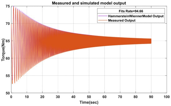
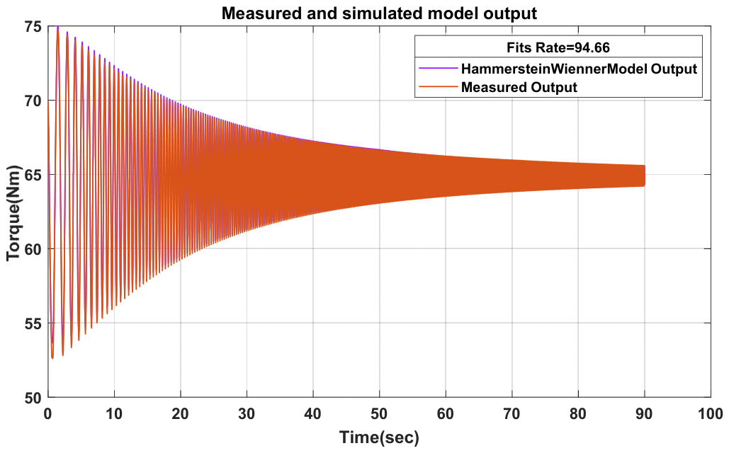
In the model configuration, the nonlinearity function is selected as a piecewise linear function and the linear block is selected as the 2 zeros 2 poles transfer function. The Hammerstein–Wiener model reached 94.65% fitting rate as seen in Figure 14.

Figure 14. Hammerstein–Wiener model system identification result.

5. Model Validation

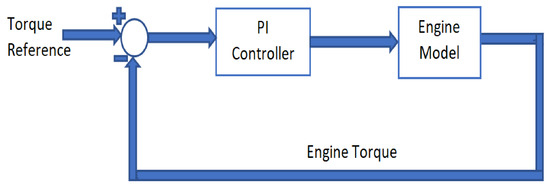
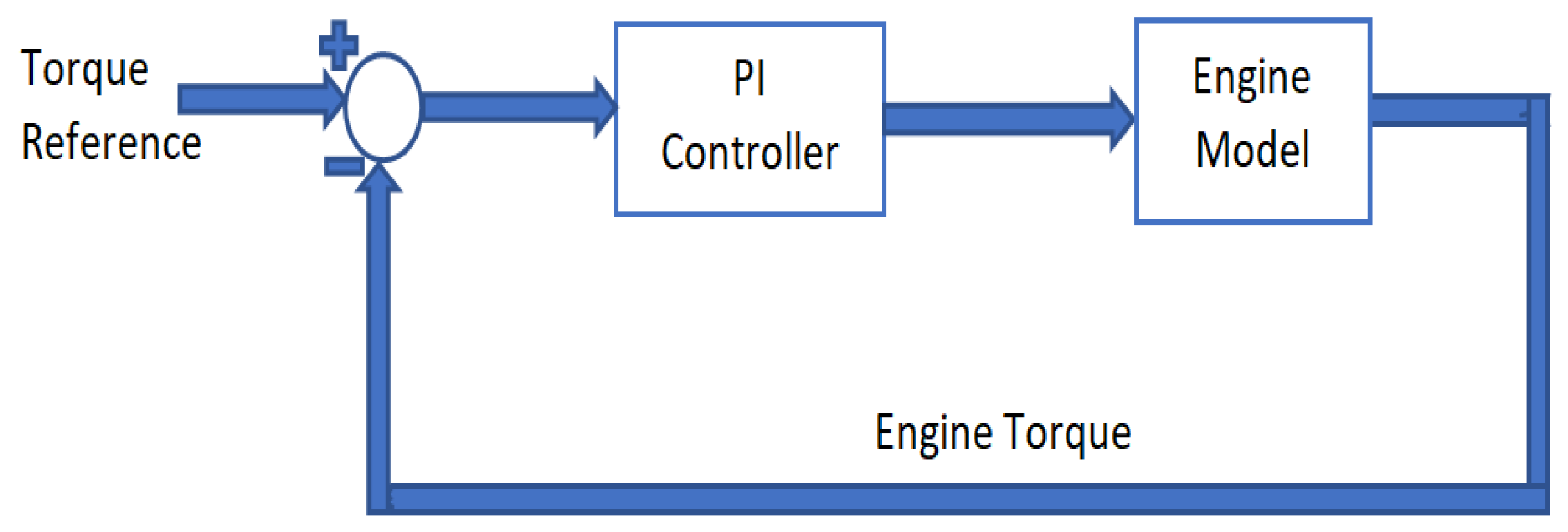
Three system identification models are validated on closed-loop performance with the same PI controller coefficient. Engine torque closed-loop model is created in Simulink as seen in Figure 15. Then engine model block is replaced with the State-Space, nonlinear ARX, Hammerstein–Wiener model and engine dynamic model respectively.

Figure 15. Engine models’ closed-loop diagram.

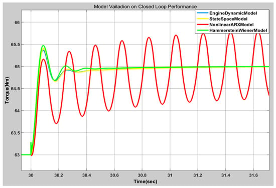
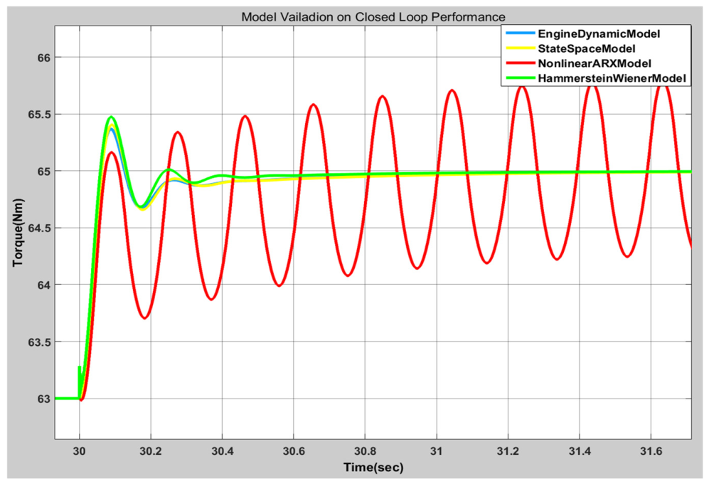
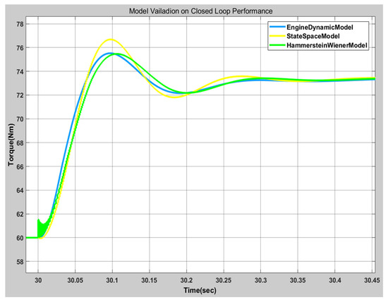
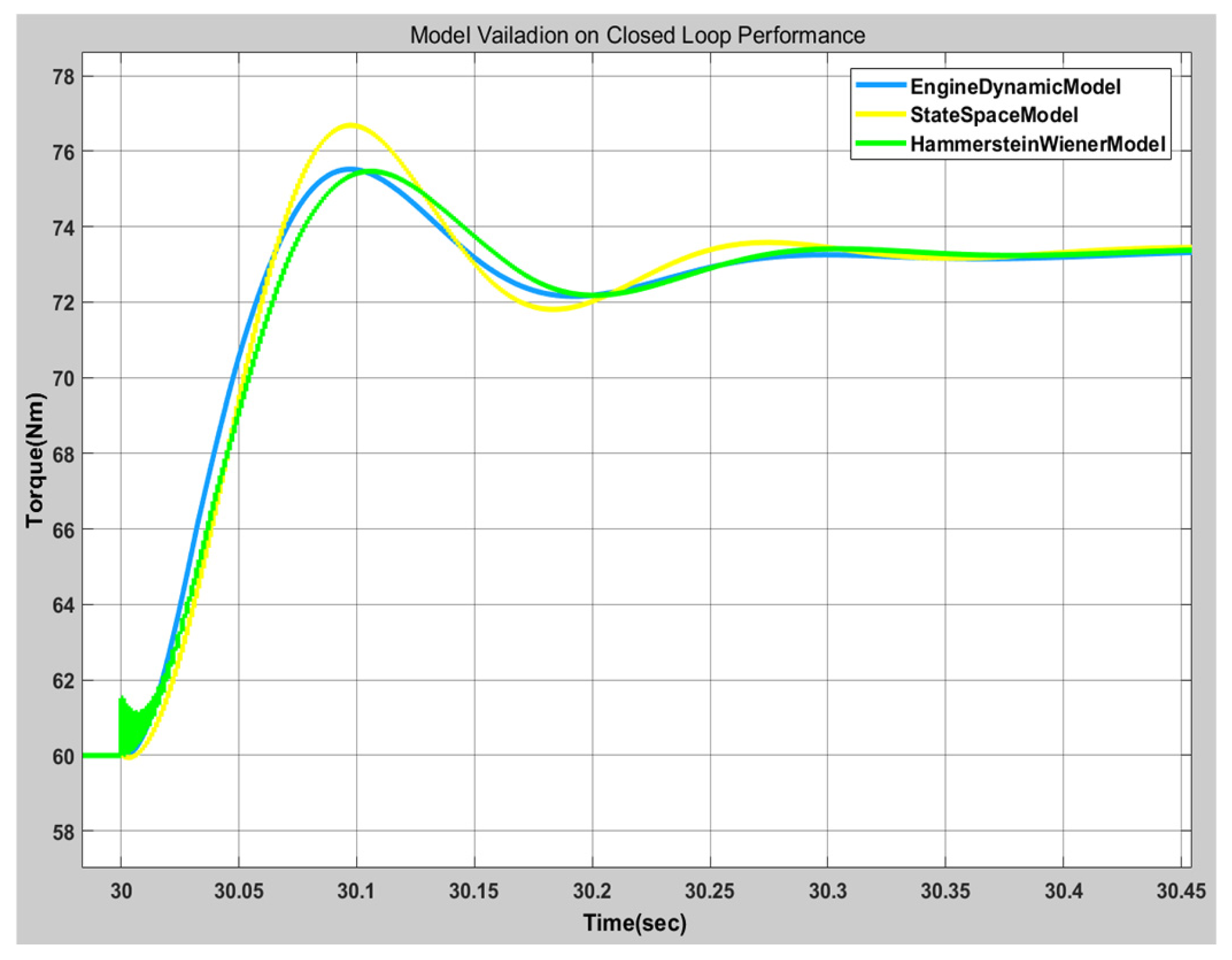
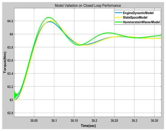
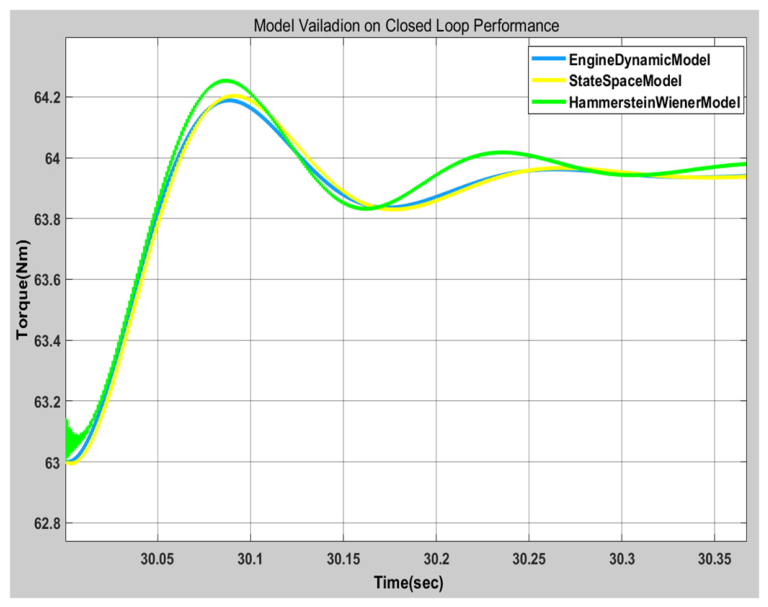
The closed-loop responses are compared based on step response characteristics. The graphical results are presented in Figure 16, Figure 17 and Figure 18. To quantitatively evaluate model accuracy, the Root Mean Square Error (RMSE), defined in Equation (21), is used and the results are reported in Table 5, Table 6 and Table 7.

$$RMS{E}_{IdentificationModel}=\sqrt{{\displaystyle \frac{1}{N}}{\sum }_{k=1 }^N{{(y}_{EngDynamicModel}\left(k\right)-y_{IdentificationModel}\left(k\right))}^2 }$$

(21)

$$y_{EngDynamicModel}\left(k\right)=\mathrm{e}\mathrm{n}\mathrm{g}\mathrm{i}\mathrm{n}\mathrm{e} \mathrm{d}\mathrm{y}\mathrm{n}\mathrm{a}\mathrm{m}\mathrm{i}\mathrm{c} \mathrm{m}\mathrm{o}\mathrm{d}\mathrm{e}\mathrm{l} \mathrm{o}\mathrm{u}\mathrm{t}\mathrm{p}\mathrm{u}\mathrm{t}$$

$$y_{IdentificationModel}\left(k\right)=\mathrm{i}\mathrm{d}\mathrm{e}\mathrm{n}\mathrm{t}\mathrm{i}\mathrm{f}\mathrm{i}\mathrm{c}\mathrm{a}\mathrm{t}\mathrm{i}\mathrm{o}\mathrm{n} \mathrm{m}\mathrm{o}\mathrm{d}\mathrm{e}\mathrm{l} \mathrm{o}\mathrm{u}\mathrm{t}\mathrm{p}\mathrm{u}\mathrm{t}$$

$$N=total number of sample$$

Figure 16. Closed-loop response of models.

Figure 17. Closed-loop response of model at 60–74 nm reference.

Figure 18. Closed-loop response of models at 63–64 nm reference.

Table 5. Closed-loop RMSE comparison of identification models.

Model	RMSE (Nm)
State-Space	0.0144
Nonlinear ARX	0.5695
Hammerstein-Wienner	0.0389

Table 6. Closed-loop RMSE comparison of identification models at 60–74 nm reference.

Model	RMSE (Nm)
State-Space	0.5241
Hammerstein–Wiener	0.4313

Table 7. Closed-loop RMSE comparison of identification models at 63–64 Nm reference.

Model	RMSE (Nm)
State-Space	0.0126
Hammerstein–Wiener	0.0405

The nonlinear ARX model’s closed-loop response is prone to oscillation in some torque ranges. Therefore, it is negatively distinguished from the other models. The State-Space and Hammerstein–Wiener models provide adequate response at all torque ranges.

In conclusion, the State-Space and Hammerstein–Wiener models provide adequate closed-loop validation. The Hammerstein–Wiener model shows better performance at the high torque reference step as seen in Figure 17. The State-Space model shows better performance at the small torque reference step as seen in Figure 18. The State-Space model is used for the cruise controller design in the following sections.

6. Cruise Controller Design

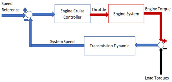
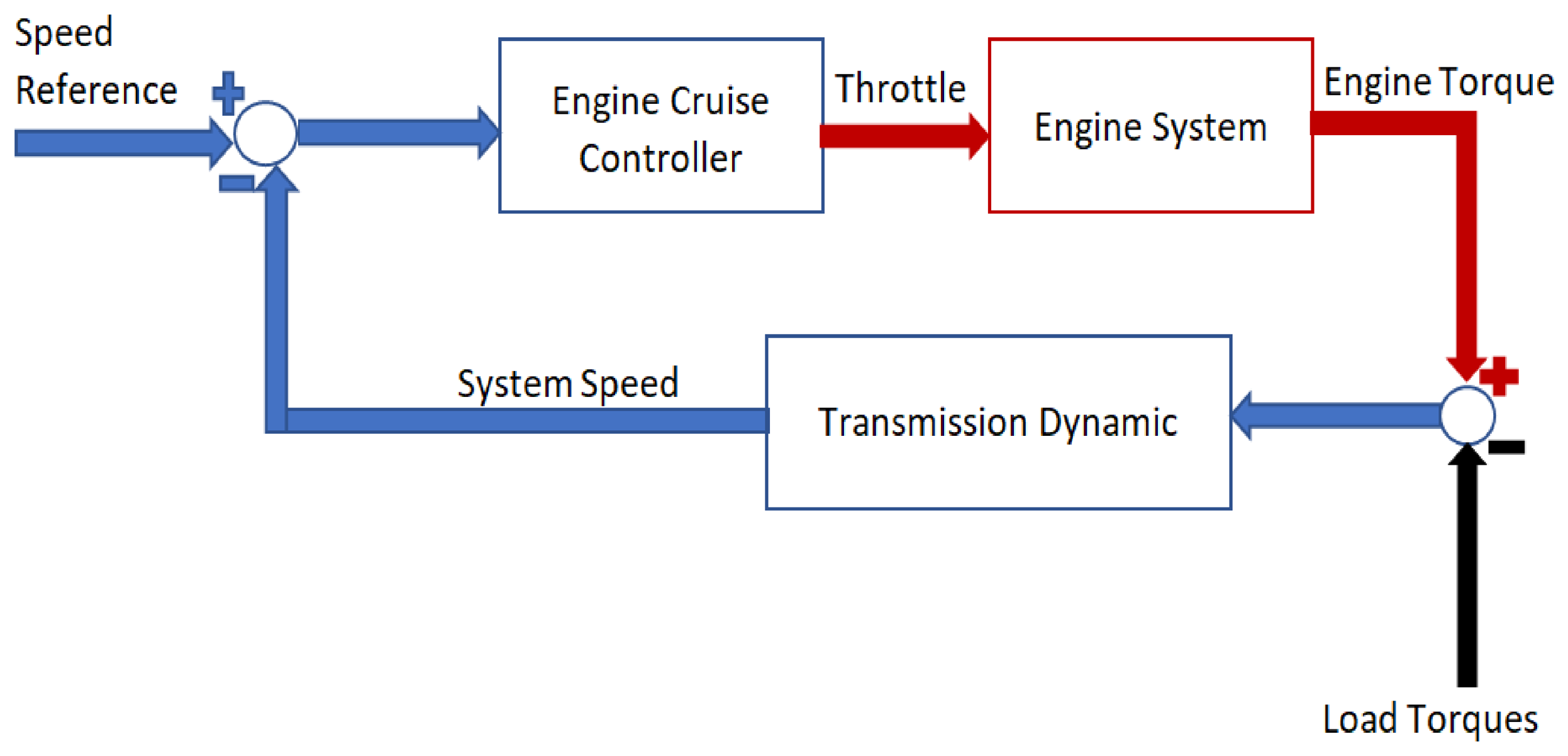
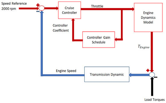
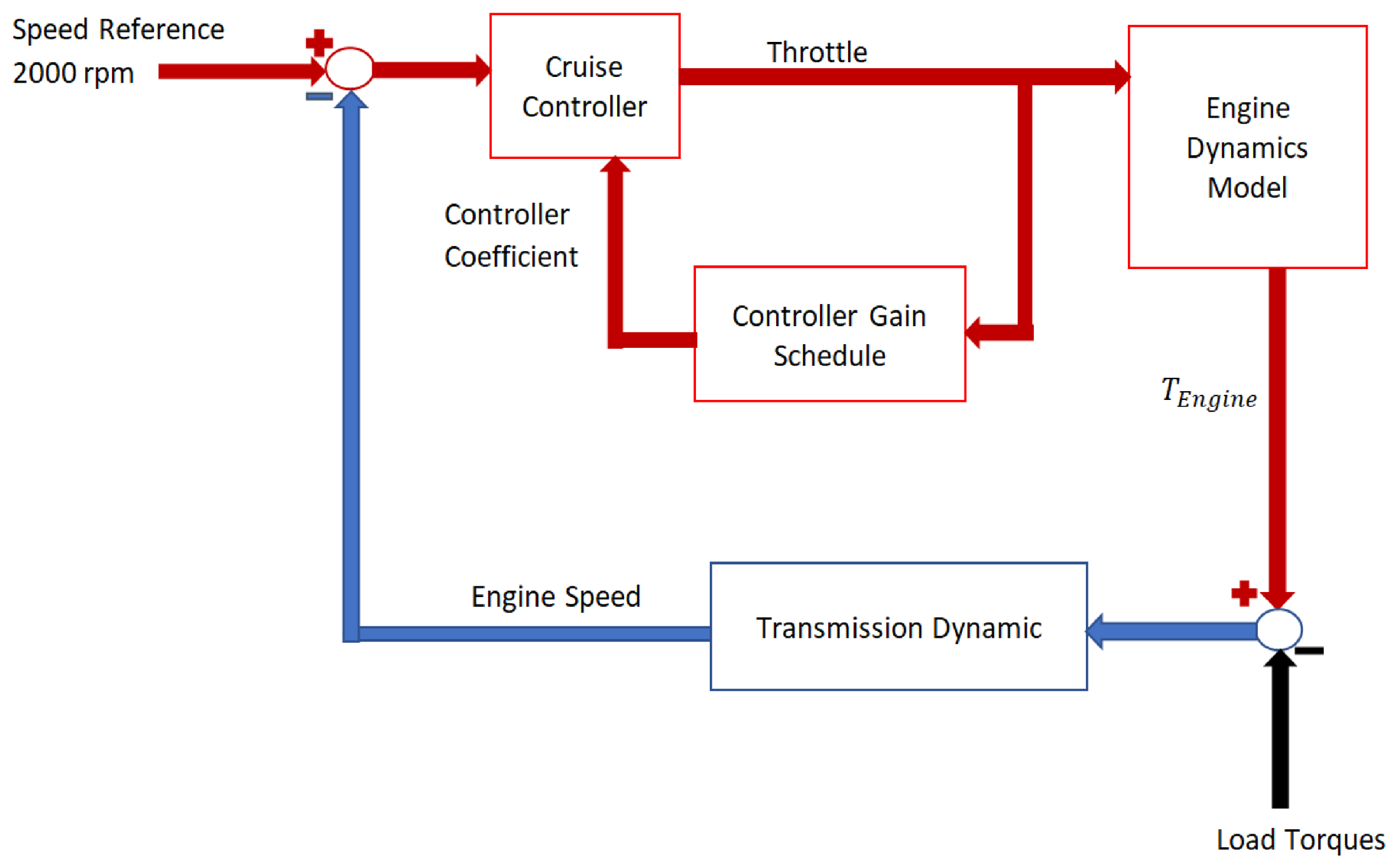
The piston engine speed controller has been investigated by previous research [32,33,34]. In this work, the cruise control concept is implemented on a piston engine, as shown in Figure 19. The cruise controller maintains the engine speed at constant reference values [34,35]. The controller is deployed after the system reaches reference speed; then, it preserves system speed against load torque.

Figure 19. Cruise controller model diagram.

Load torques change during operation. For example, in vehicle drive applications, it changes alongside drive characteristics [32], in generator applications, it changes with load current [33] and in aircraft applications, it changes alongside flight characteristics [36]. Cruise control conserves system speed against drastic load torque changes. The dynamic model of the piston engine relating throttle to torque, based on the State-Space formulation, has been obtained in previous work. The piston engine dynamic system strongly depends on air flow which is adjusted by throttle level. Therefore, system dynamics change with throttle angle. Deploying a single PID controller could not achieve an adequate response. Thus gain scheduling controller is deployed.

Gain Schedule Controller

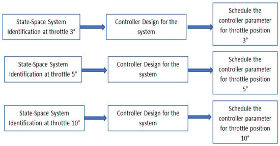
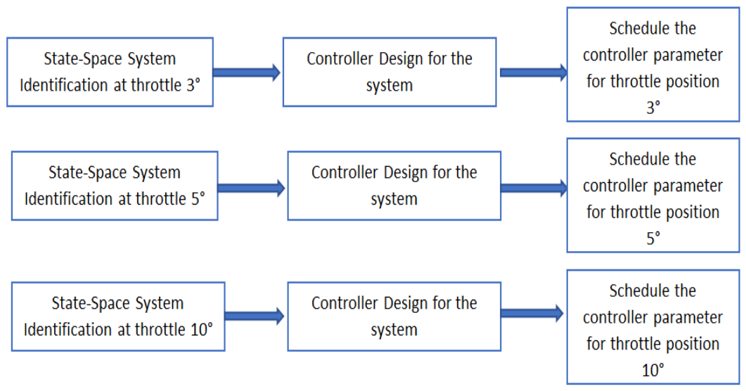
The gain schedule method is widely used to control complex nonlinear systems [37,38]. In gain schedule control, different operation points are determined; then, sufficient control is designed for these points. Controller gains are interpolated between designed controller gains according to operation point changes during operation [35,36]. The gain schedule controller is used when a single controller set cannot provide sufficient performance throughout the entire operation range. In a gain schedule controller, the nonlinear plant is linearized at different operation points, then the linear controller parameters are tuned on linearized plants. The controller gains are scheduled according to operation points [39]. In progress work, State-Space system identification models are used instead of linearized models. The operation points are adjusted by throttle angle such as 3°, 5° and 10°. The State-Space system identification process is repeated at these three different throttle angles. Then, the PID controller is tuned based on these system identification models, as shown in Figure 20.

Figure 20. Gain schedule controller design process.

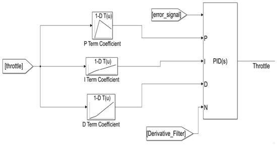
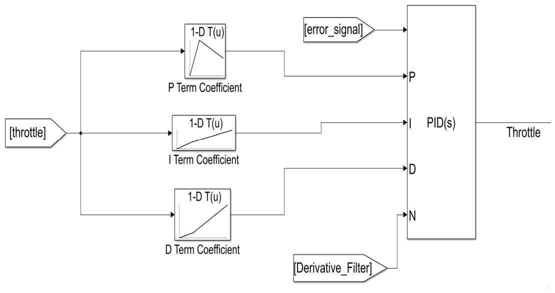
After designing a PID controller for three throttle positions (3°, 5° and 10°) with disturbance rejection criteria, the PID coefficients are scheduled with a throttle signal as seen in Figure 21. The overall gain scheduled cruise controller design diagram is shown in Figure 22. Cruise control maintains the system speed at 2000 rpm, the controller’s coefficients are interpolated with the throttle angle as seen in Figure 22 and the load profile changes during operation.

Figure 21. Gain schedule controller Simulink implementation.

Figure 22. Gain scheduling cruise controller diagram.

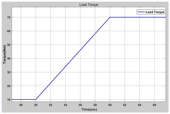
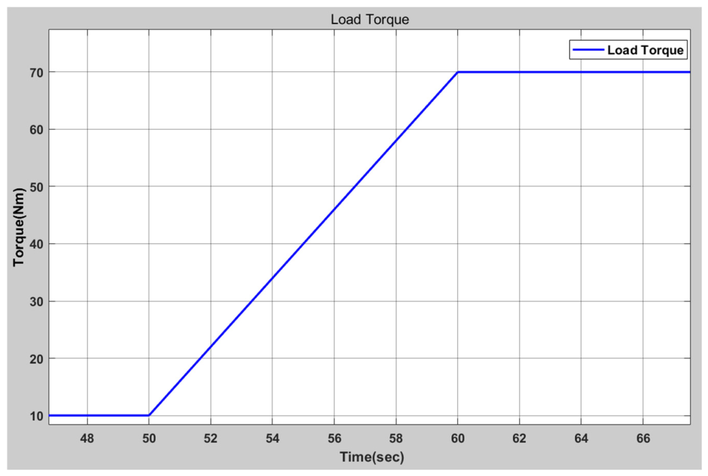
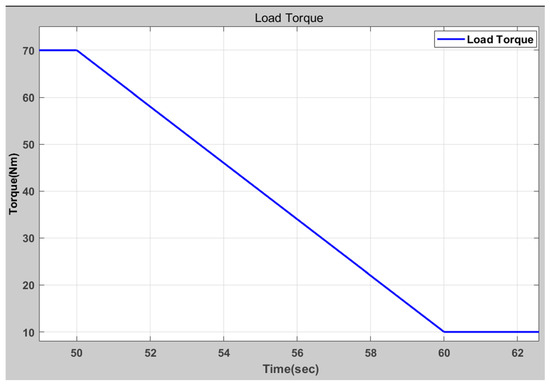
The load torque profile is selected as a ramp profile which increases from 10 Nm to 70 Nm in 10 s as seen in Figure 23 and decreases from 70 Nm to 10 Nm in 10 s as seen in Figure 24.

Figure 23. Load torque ramp-up profile.

Figure 24. Load torque ramp-down profile.

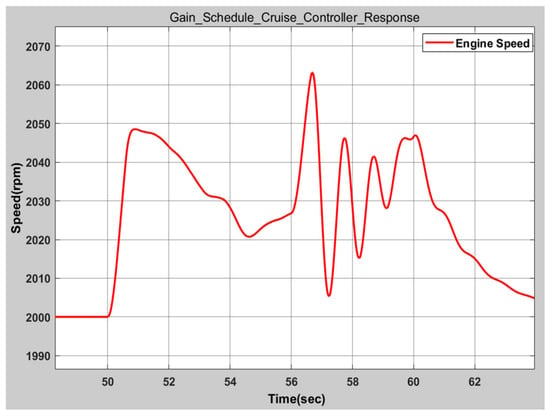
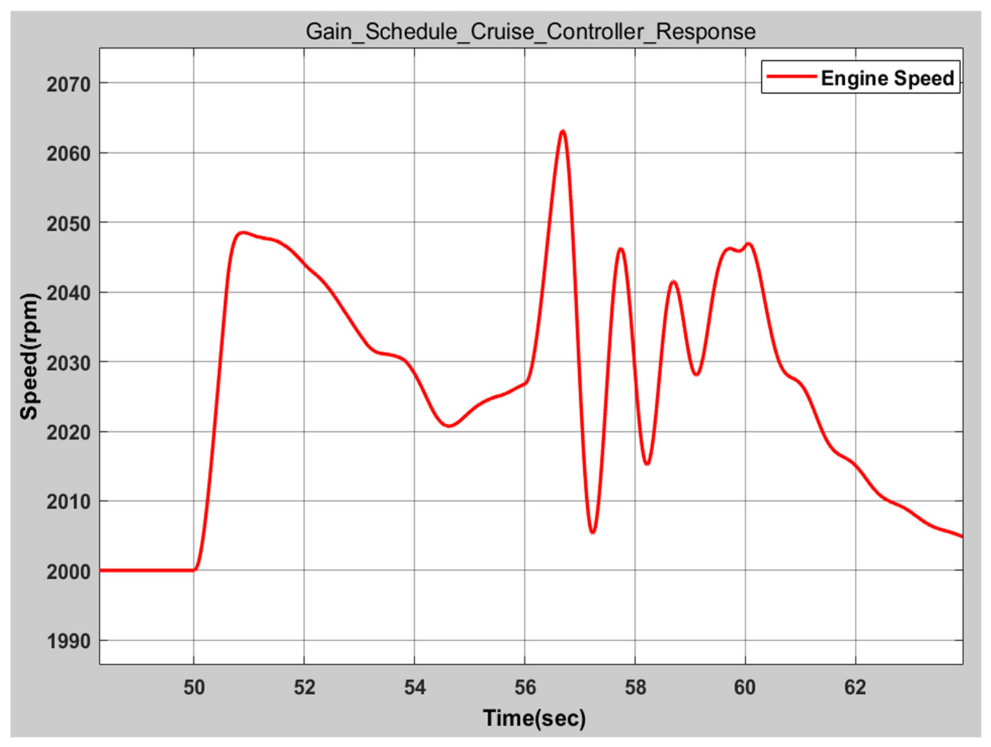
Gain scheduling cruise controller rejects ramp-up load torque disturbance in 17 s and deviates at a maximum of 50 rpm from reference speed as seen in Figure 25.

Figure 25. Gain scheduled cruise controller engine speed response against ramp-up load profile.

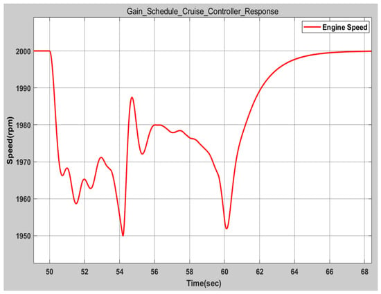
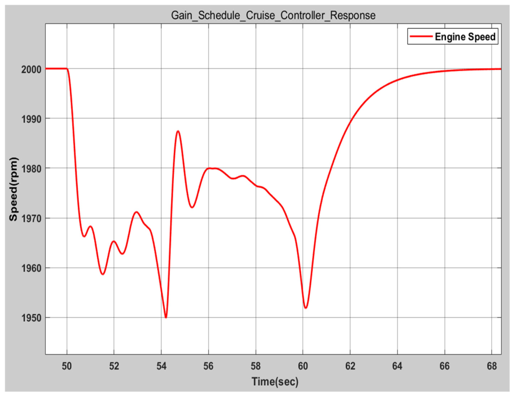
Gain scheduled cruise controller rejects ramp-down load torque disturbance in 16 s and deviates at a maximum of 62 rpm from the reference speed, as seen in Figure 26.

Figure 26. Gain scheduled cruise controller engine speed response against ramp-down load profile.

7. Disturbance Observer Design

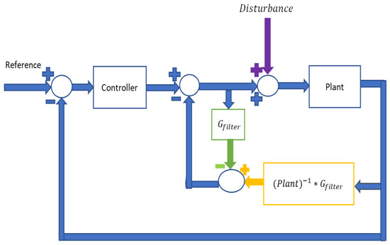
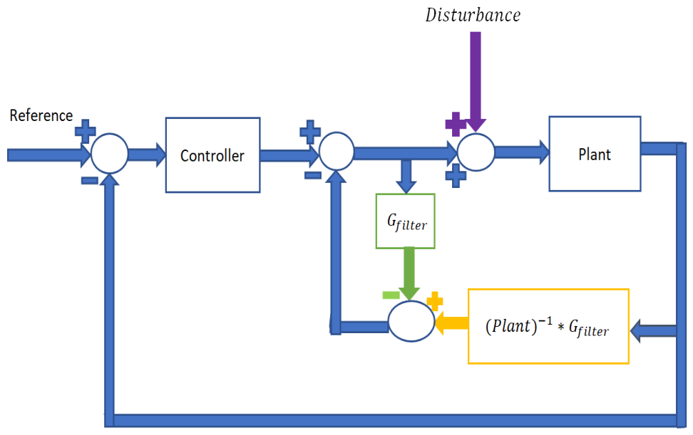
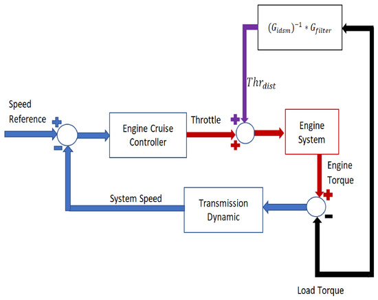
In the general disturbance observable concept, the disturbance is added to plant input, as seen in Figure 27, but in the cruise controller concept, the disturbance is added to engine torque. Therefore, classic disturbance observable method is not proper for the cruise controller.

Figure 27. Classical disturbance observer design.

The disturbance observer helps the controller to overcome disturbance effect. In this work, a disturbance observer is designed for measurable load torques and unmeasurable load torques. ${Thr}_{dist}$ command is added to throttle, the command compensate load torque effect. ${Thr}_{dist}$ is expressed at Equation (22).$G_{filter}$ is added to make the ${{(G}_{idsm})}^{-1} \ast G_{filter}$ term causal. The corresponding block diagram is shown in Figure 28.

$${Thr}_{dist}=Loa{d}_{torque} \ast {{(G}_{idsm})}^{-1} \ast G_{filter}$$

(22)

$$G_{idsm}=System Identified Engine Model$$

$$G_{filter}=Low pass filter$$

$$Loa{d}_{torque}=External load torque$$

Figure 28. Disturbance observer design for measurable load torque.

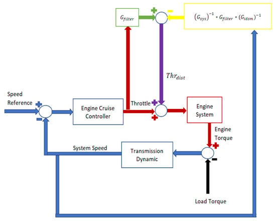
If load torque is unmeasurable, throttle compensation is applied based on the system speed using the following equations.

$$\left(spd\right) \ast {{(G}_{sys})}^{-1} \ast G_{filter}={(T}_{eng}-T_{load}) \ast G_{filter}$$

(23)

$$T_{eng}\cong thr \ast G_{idsm}$$

$$thr \ast G_{idsm} \ast G_{filter}-\left(spd\right) \ast {{(G}_{sys})}^{-1} \ast G_{filter} \cong T_{load} G_{filter}$$

(24)

$$th{r}_{dis}=T_{load} \ast G_{filter} \ast {G_{idsm}}^{-1}$$

(25)

In Equation (24), both sides is multiply with ${{ G}_{idsm}}^{-1}$

$$thr \ast G_{filter}-\left(spd\right) \ast {{(G}_{sys})}^{-1} \ast G_{filter} \ast {G_{idsm}}^{-1} \cong T_{load} \ast G_{filter}{{ \ast G}_{idsm}}^{-1}=th{r}_{dis}$$

$$th{r}_{dis}=thr \ast G_{filter}-\left(spd\right) \ast {{(G}_{sys})}^{-1} \ast G_{filter} \ast {G_{idsm}}^{-1}$$

(26)

$G_{filter}$ is selected to guarantee that the $\left(spd\right) \ast {{(G}_{sys})}^{-1} \ast G_{filter} \ast {G_{idsm}}^{-1}$ term is causal. It could be second-degree or a higher degree. The $th{r}_{dis}$ command is derived from system-measured values and parameters, as defined in Equation (26). Figure 29 presents the block diagram of the disturbance observer for non-measurable load torque.

Figure 29. Disturbance observer design for unmeasurable load torque.

Non-Minimum Phase Criteria

The disturbance observer design method is limited to a minimum phase system, which means that all poles and zeros are inside a stable region. Designing a disturbance observer for a non-minimum phase system which has an unstable zero is a challenging process. Although some research focuses on disturbance observers for non-minimum phase systems, the research includes additional design and mathematical processes [40,41]. The State-Space system identification method reaches non-minimum phase models. Therefore, a transfer function identification model is used to guarantee that the model is minimum-phase for disturbance observer design. A third-degree one-zero minimum phase transfer function model is used ${(G}_{idsm})$ and a second-degree high-cutoff frequency filter is used as $G_{filter}$.

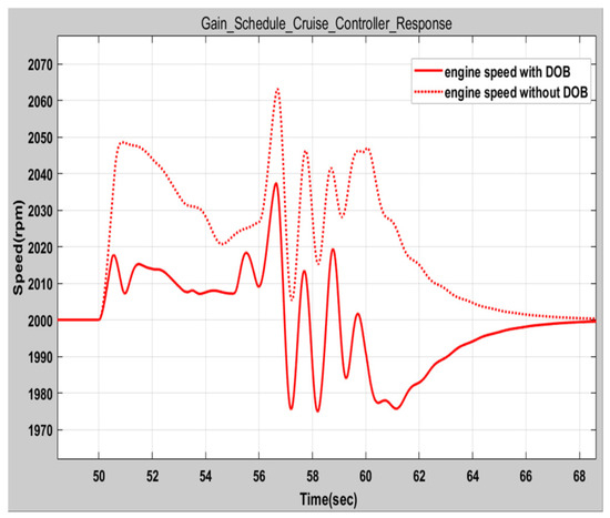
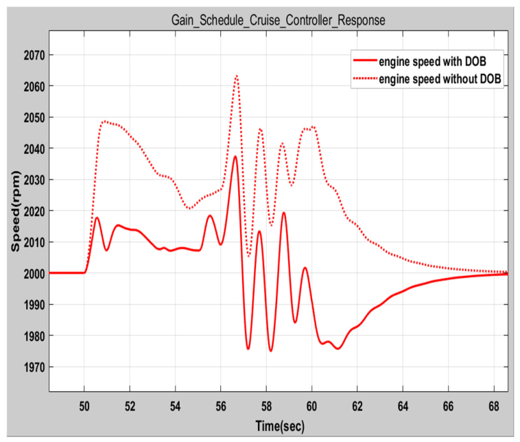
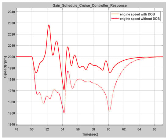
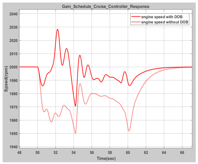
Disturbance observer design improves cruise controller response, as seen in Figure 30; maximum deviation is reduced from 62 rpm to 37 rpm with disturbance observer design against ramp-down load profile. Similarly, against ramp-up profile, the disturbance observer design reduces maximum deviation from 50 rpm to 28 rpm, as seen in Figure 31. In addition, the control performance is further quantified using the reference tracking error (RMSE), which also demonstrates improved performance with the disturbance observer method as shown in Table 8 and Table 9. The RMSE of the reference tracking error is defined in Equation (27).

$$RMS{E}_{referencetralinerror}=\sqrt{{\displaystyle \frac{1}{N}}\sum _{k=1 }^N{r\left(k\right)-y\left(k\right))}^2 }$$

(27)

$$r\left(k\right)=cruise reference speed(2000 rpm)$$

$$y\left(k\right)=engine speed$$

$$N=Number of sample$$

Figure 30. Cruise controller with disturbance observer against ramp-down load profile.

Figure 31. Cruise controller with disturbance observer against ramp-up profile.

Table 8. Performance comparison under ramp-down load profile.

Method	Maximum Speed Deviation (rpm)	Reference Tracking Error RMSE (rpm)
Gain Scheduling	62	27.72
Gain Scheduling + Disturbance Observer	37	12.7

Table 9. Performance comparison under ramp-up load profile.

Method	Maximum Speed Deviation (rpm)	Reference Tracking Error RMSE (rpm)
Gain Scheduling	50	26.29
Gain Scheduling + Disturbance Observer	28	9.36

8. Conclusions

In this work, the system identification process is applied on a piston engine–dynamometer system while the system is operated in closed-loop mode. The piston engine’s throttle is a measurable value. But obtaining engine torque is not possible due to noncausality; therefore, a high-cutoff frequency low pass filter is deployed to overcome noncausality. Engine torque is derived from a closed-loop model by using known parameters and measured values. System identification is applied on throttle to engine torque and three identification methods are used. Identification models are validated on their closed-loop performance. Although the nonlinear ARX model reached the highest fitting rate, the State-Space and Hammerstein–Wiener models achieve more correlated results in closed-loop validation. Thus, the State-Space model has been chosen for cruise controller design. Piston engine dynamics changed with throttle angle, thus one single PID coefficient could not provide adequate response; therefore, gain schedule concepts are deployed. Finally, the disturbance observer method is deployed to improve cruise controller performance. Classical disturbance observable design is not proper for this case. Therefore, the disturbance observable design is reshaped for this case. State-Space model identification reaches a non-minimum phase which is not suitable for a disturbance observer. Thus, instead of a State-Space model, a transfer function model is used for the disturbance observer. In this manner, the identified model is granted to be a minimum phase system. Disturbance observer improves cruise controller response in simulation response.

References

- Jiang, H.; Zhou, Y.; Ho, H.W.; Abu Bakar, E. Modeling of two-stroke aviation piston engines for control applications. Adv. Mech. Eng. 2023, 15, 16878132231153234. [Google Scholar] [CrossRef] [Scilit]
- Carbot-Rojas, D.; Escobar-Jiménez, R.; Gómez-Aguilar, J.; Téllez-Anguiano, A. A survey on modeling, biofuels, control and supervision systems applied in internal combustion engines. Renew. Sustain. Energy Rev. 2017, 73, 1070–1085. [Google Scholar] [CrossRef] [Scilit]
- Crossley, P.R.; Cook, J.A. A nonlinear engine model for drivetrain system development. In International Conference on Control; IET: Auburn Hills, MI, USA, 1991; pp. 921–925. [Google Scholar]
- Zhihu, W.; Run, P. Torque based spark ignition engine and powertrain modeling. In 7th World Congress on Intelligent Control and Automation; IEEE: New York, NY, USA, 2008. [Google Scholar]
- Tan, Y.; Saif, M. Neural-networks-based nonlinear dynamic modeling for automotive engines. Neurocomputing 2000, 30, 129–142. [Google Scholar] [CrossRef] [Scilit]
- Yu, M.; Tang, X.; Lin, Y.; Wang, X. Diesel engine modeling based on recurrent neural networks for a hardware-in-the-loop simulation system of diesel generator sets. Neurocomputing 2018, 283, 9–19. [Google Scholar] [CrossRef] [Scilit]
- Zhai, Y.; Qian, K.; Xue, F.; Tayahi, M. Modelling of automotive engine dynamics using diagonal recurrent neural network. J. Univers. Comput. Sci. 2018, 24, 1330–1342. [Google Scholar]
- Ren, Y. Torque Prediction of Internal Combustion Engines Based on Time Series. In Proceedings of the 2025 2nd International Conference on Image Processing, Intelligent Control and Computer Engineering; Association for Computing Machinery: New York, NY, USA, 2025. [Google Scholar]
- Gölcü, M.; Sekmen, Y.; Erduranlı, P.; Salman, M.S. Artificial neural-network based modeling of variable valve-timing in a spark-ignition engine. Appl. Energy 2005, 81, 187–197. [Google Scholar] [CrossRef] [Scilit]
- Buşoniu, L.; de Bruin, T.; Tolić, D.; Kober, J.; Palunko, I. Reinforcement learning for control: Performance, stability, and deep approximators. Annu. Rev. Control. 2018, 46, 8–28. [Google Scholar] [CrossRef] [Scilit]
- Dai, H.; Landry, B.; Yang, L.; Pavone, M.; Tedrake, R. Lyapunov-stable neural-network control. arXiv 2021, arXiv:2109.14152. [Google Scholar]
- ArjomandBigdeli, A.; Mata, A.; Bak, S. Verification of neural network control systems in continuous time. In International Symposium on AI Verification; Springer Nature: Cham, Switzerland, 2024. [Google Scholar]
- Bunker, B.J.; Franchek, M.A.; Thomason, B.E. Robust multivariable control of an engine-dynamometer system. IEEE Trans. Control. Syst. Technol. 1997, 5, 189–199. [Google Scholar] [CrossRef] [Scilit]
- Lamara, A.; Lanusse, P.; Charlet, A.; Gruel, D.N.; Colin, G.; Lesobre, A.; Oustaloup, A.; Chamaillard, Y. High dynamic engine-dynamometer identification and control. IFAC Proc. Vol. 2014, 47, 5217–5222. [Google Scholar] [CrossRef] [Scilit]
- Erdogan, D.; Jakubek, S.; Mayr, C.; Hametner, C. Combustion engine test bed system identification under the presence of cyclic disturbances. IEEE Trans. Ind. Electron. 2020, 68, 8636–8645. [Google Scholar] [CrossRef] [Scilit]
- Tan, J.; Xue, S.; Li, H.; Guo, Z.; Cao, H.; Li, D. Prescribed performance robust approximate optimal tracking control via Stackelberg game. IEEE Trans. Autom. Sci. Eng. 2025, 22, 12871–12883. [Google Scholar] [CrossRef] [Scilit]
- Tan, J.; Xue, S.; Guan, Q.; Guo, Z.; Cao, H.; Chen, B. Fixed-time stochastic learning from human-UAV interaction with state-input constraints. IEEE Trans. Ind. Electron. 2025, 73, 3071–3082. [Google Scholar] [CrossRef] [Scilit]
- Grobbelaar, E. The Development of a Small Diesel Engine Test Bench Employing an Electric Dynamometer. Master’s Thesis, Stellenbosch University, Stellenbosch, South Africa, 2017. [Google Scholar]
- The MathWorks Inc. Calibrate, Validate, and Optimize SI Engine with Dynamometer Test Harness. 2025. Available online: https://ww2.mathworks.cn/help/autoblks/ug/explore-the-si-engine-dynamometer-reference-application.html (accessed on 10 April 2026).
- Niemann, H.; Miklos, R.; Poulsen, N.K. Grey box identification in closed-loop. In American Control Conference (ACC); IEEE: New York, NY, USA, 2019. [Google Scholar]
- Mandloi, R.; Pritesh, S. Methods for closed loop system identification in industry. J. Chem. Pharm. Res. 2015, 7, 892–896. [Google Scholar]
- Shah, P.; Sekhar, R. Closed loop system identification of a DC motor using fractional order model. In International Conference on Mechatronics, Robotics and Systems Engineering; IEEE: New York, NY, USA, 2019. [Google Scholar]
- Dou, L.; Zong, Q.; Sun, L.; Ji, Y. Excitation signal design for closed-loop system identification. In Chinese Control and Decision Conference; IEEE: New York, NY, USA, 2009. [Google Scholar]
- Shim, H. Disturbance observers. In Encyclopedia of Systems and Control; Springer: Cham, Switzerland, 2021; pp. 622–629. [Google Scholar]
- Wai, C.K.; Rong, Y.Y.; Morris, S. Simulation of a distance estimator for battery electric vehicle. Alex. Eng. J. 2015, 54, 359–371. [Google Scholar] [CrossRef] [Scilit]
- Glass, J.; Franchek, M. NARMAX modelling and robust control of internal combustion engines. Int. J. Control 1999, 72, 289–304. [Google Scholar] [CrossRef] [Scilit]
- Zito, G.; Landau, I. NARMAX model identification of a variable geometry turbocharged diesel engine. In American Control Conference; IEEE: New York, NY, USA, 2005. [Google Scholar]
- Mottin, T.; Oroski, E.; Carlos, T.M.; Silveira, L.B.; Alegre, J.A.A.V. Nonlinear system identification of a homogeneous charge compression ignition engine. In Proceedings of the Simpósio Brasileiro de Automação Inteligente—SBAI, Manaus, Brazil, 15–18 October 2023. [Google Scholar]
- Jamaludin, I.W.; Wahab, N.A.; Khalid, N.S.; Sahlan, S.; Ibrahim, Z.; Rahmat, M.F. N4SID and MOESP subspace identification methods. In IEEE Colloquium on Signal Processing; IEEE: New York, NY, USA, 2013. [Google Scholar]
- The MathWorks Inc. What Are Nonlinear ARX Models? 2025. Available online: https://ww2.mathworks.cn/help/ident/ug/what-are-nonlinear-arx-models.html (accessed on 10 April 2026).
- The MathWorks Inc. Hammerstein-Wiener Models. 2025. Available online: https://ww2.mathworks.cn/help/ident/hammerstein-wiener-models.html (accessed on 10 April 2026).
- Li, Y.; He, L. Counterbalancing speed control for hydrostatic drive heavy vehicle under long down-slope. IEEE/ASME Trans. Mechatron. 2015, 20, 1533–1542. [Google Scholar] [CrossRef] [Scilit]
- Iwanski, G.; Bigorajski, Ł.; Koczara, W. Speed control with incremental algorithm of minimum fuel consumption tracking for variable speed diesel generator. Energy Convers. Manag. 2018, 161, 182–192. [Google Scholar] [CrossRef] [Scilit]
- Khayyam, H.; Nahavandi, S.; Davis, S. Adaptive cruise control look-ahead system for energy management of vehicles. Expert Syst. Appl. 2012, 39, 3874–3885. [Google Scholar] [CrossRef] [Scilit]
- Huo, H.; Li, J. Cruise control based on gain scheduling PI diesel engine speed controller. In IEEE International Vehicle Electronics Conference; IEEE: New York, NY, USA, 1999. [Google Scholar]
- Shams, T.A.; Shah, S.I.A.; Khushbash, S.; Ahmad, M.A. Evaluation of aerodynamic and stability performance parameters of high wing piston engine aircraft. In 2019 16th International Bhurban Conference on Applied Sciences and Technology (IBCAST), Islamabad, Pakistan, 8–12 January 2019; IEEE: New York, NY, USA, 2019. [Google Scholar]
- Liu, Z.; Gou, L.; Fan, D.; Zhou, Z. Design of gain-scheduling robust controller for aircraft engine. In Chinese Control Conference; IEEE: New York, NY, USA, 2019. [Google Scholar]
- Gou, L.; Liu, Z.; Fan, D.; Zheng, H. Aeroengine robust gain-scheduling control based on performance degradation. IEEE Access 2020, 8, 104857–104869. [Google Scholar] [CrossRef] [Scilit]
- The MathWorks Inc. Gain Scheduling. 2025. Available online: https://ww2.mathworks.cn/discovery/gain-scheduling.html (accessed on 10 April 2026).
- Son, Y.I.; Shim, H.; Jo, N.H.; Kim, S.-J. Design of disturbance observer for non-minimum phase systems using PID controllers. In SICE Annual Conference; IEEE: New York, NY, USA, 2007. [Google Scholar]
- Jo, N.H.; Shim, H.; Son, Y.I. Disturbance observer for non-minimum phase linear systems. Int. J. Control Autom. Syst. 2010, 8, 994–1002. [Google Scholar] [CrossRef] [Scilit]
Disclaimer/Publisher’s Note: The statements, opinions and data contained in all publications are solely those of the individual author(s) and contributor(s) and not of MDPI and/or the editor(s). MDPI and/or the editor(s) disclaim responsibility for any injury to people or property resulting from any ideas, methods, instructions or products referred to in the content. |
© 2026 by the authors. Licensee MDPI, Basel, Switzerland. This article is an open access article distributed under the terms and conditions of the Creative Commons Attribution (CC BY) license.