Warehouse Mobile Robot Path Planning Performance Sensitivity to the Neighbor Radius Parameter

Abstract

Many RRT*-based sampling path planning algorithms consider neighboring nodes around a newly added node. The neighbor radius parameter $r_{near}$ determines which nodes are included. The performance of RRT*-based algorithms can vary significantly with $r_{near}$. This variation can weaken generalization across environments. This paper quantitatively analyzes the effect of $r_{near}$ on performance in sampling-based path planning for mobile robots in a warehouse environment. We evaluate RRT*-based algorithms by varying $r_{near}$. We then select the heuristic chosen $r_{near}$ for each algorithm and compare the algorithms under the same conditions. Experiments are conducted in a warehouse environment with a fixed start position and five goal positions. Performance is evaluated using planning time, path length, and cumulative change in turning angle. Lower values indicate better performance for all three metrics. Based on the experimental results, we derive a heuristic value of $r_{near}$ for each case. We also identify algorithm characteristics in computational efficiency and path quality under the heuristically chosen parameter settings. The final goal of this study is to provide quantitative evidence for selecting $r_{near}$ in warehouse applications. We also present guidelines for parameter setting and algorithm selection for RRT*-based sampling path planning.

1. Introduction

Science and technology development affects most of our lives. In particular, there are many attempts for robots to replace tasks that humans used to do. For example, in hospitals, there are cases where an autonomous driving robot transports specimens instead of medical staff [1] or makes rounds remotely [2]. Also, in the agricultural field, there are cases where crops are harvested with an autonomous driving tractor [3] or a weeding robot performs repetitive tasks such as weed removal [4]. There are also such cases in warehouses. For example, there are unloading robots that take logistics items out from inside containers or trucks [5], and inside a warehouse, when a worker puts items in a specific area, a picking assistance robot transports them to the depot instead of the worker, reducing the worker’s walking distance and fatigue [6]. Such robot technologies reduce workers’ burden and improve throughput and work safety. In addition, a method for monitoring the inside of a warehouse using drones has also been proposed.

Robots used in warehouses move for their own tasks. In order for robots to move, they have to calculate a path from the current position to the position they want to go to. Calculating such a robot’s moving path is called path planning. Path planning is used not only for movement but also to avoid suddenly appearing dynamic obstacles. For this, path planning must calculate a path as fast as possible while calculating an optimal path [7].

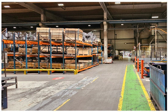
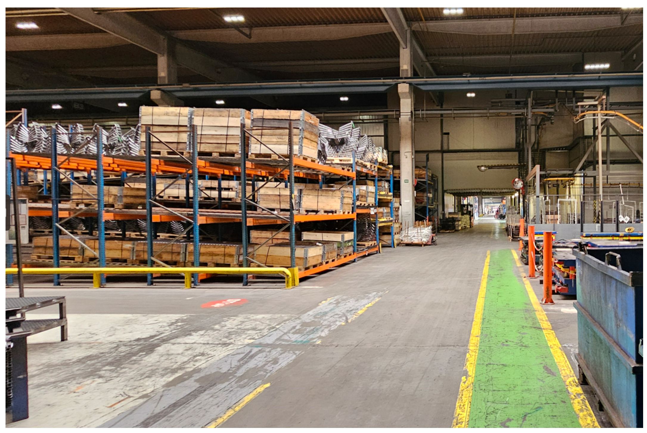
In this study, among path planning algorithms, we aim to compare the performance of RRT*-based algorithms among sampling-based algorithms known to be fast. RRT*-based algorithms are widely used due to their fast path planning speed. However, in such RRT*-based algorithms, a radius parameter $r_{near}$ is used that considers neighboring nodes within a certain radius around a new node. Depending on the value of this parameter, the performance of the algorithm changes. This means that generalization becomes weaker [8]. Accordingly, selection and tuning for each algorithm parameter are required [9,10]. Therefore, to evaluate performance, we aim to compare planning time, length of path, and cumulative change in turning angle according to each parameter. Experiments are conducted targeting Quick-RRT* [11], Fast-RRT* [12], and More Quickly RRT* [13], which are known to be fast among RRT*-based algorithms. Specifically, we analyze performance according to the parameter values of the algorithms, and we aim to compare them with the heuristically chosen parameters for each algorithm. The experiments assume the path planning of robots used in warehouses. A warehouse is a facility for storing and managing items, as shown in Figure 1. The warehouse layout generally consists of repeatedly arranged racks and work areas, and is characterized by the repeated occurrence of narrow and long aisles. Therefore, although differences may exist in the detailed arrangement, the path planning of mobile robots in warehouse environments can be considered to be performed under similar structural constraints. We target four goal positions from the start position. These experiments are conducted in a ROS2 environment using the Gazebo simulator.

Figure 1. Example of the interior of a warehouse.

The goal of this study is to quantitatively analyze, for RRT*-based algorithms (Q-RRT, F-RRT*, MQ-RRT*) applied to robot path planning used in warehouse environments, the effect of the parameter $r_{near}$ on performance. Then, based on planning time, path length, and cumulative change in turning angle, we derive the heuristically chosen parameter for each algorithm and compare them with each other under the same conditions to present guidelines for selecting an algorithm and parameters suitable for logistics environments. In Section 2 of this paper, we introduce studies related to RRT*. In Section 3, we describe in detail the algorithms to be compared. In Section 4, we discuss the experimental environment and the experimental results. In Section 5, we introduce the conclusion.

2. Related Works

In path planning, classical approaches include APF (artificial potential field), cell decomposition, RRT [14], and A* [15]. Based on these representative theories, algorithms that propose improvements by applying various changes have been suggested. In the case of cell decomposition, a method that approximates curved-shaped obstacles and can be applied even when curved obstacles exist has been proposed [16]. In the case of A*, a modified algorithm has been proposed that optimizes the cost function to fit the given situation and applies dynamic updates considering temporal factors [17]. In the case of APF, a method has been proposed to solve the problem of falling into local minima during path calculation by using a water sink model [18].

Like other classical approaches, various algorithms based on RRT-based algorithms have been proposed. RRT must repeat the sampling process many times in order to guarantee the optimality of the path. However, this requires a lot of time, and the advantage of RRT, which is its fast speed, can be weakened. To solve this, RRT*, which adds a rewire process to RRT to optimize the path, was proposed. The rewire strategy proposed in RRT* complemented the lack of optimality in RRT. After that, various RRT-based algorithms were developed by introducing the rewire strategy or modifying it.

When the initial path is calculated, an ellipsoid is defined based on the start position and the goal position. Then, Informed RRT*, which is a method that improves the path by sampling within the ellipsoid range, was proposed [19]. To reflect the fact that the robot moves, RT-RRT*, which considers the changing tree’s start point during path planning, was proposed [20]. This updates the path in real time with an online tree rewiring method. AM-RRT*, which is an extended method of RT-RRT*, was proposed [21]. This increased the efficiency of finding a path by combining an assisting metric with the Euclidean distance. To speed up the path calculation speed of RRT*, RRT*-Smart, which samples in places where the path is likely to be optimized with intelligent sampling was proposed [22]. RRT*-Smart also optimized the path using the triangle inequality. Pointing out the limitations of the triangle inequality, Straight-RRT, which improved the calculation speed with a MoveParent strategy and a Straight strategy that improved it, was proposed [23].

Q-RRT* was proposed in RRT*, which considers not only the neighboring nodes of a new node but also their ancestors. F-RRT* was proposed, which performs optimal parent selection and ancestor search by optimizing the path using the considered ancestors. MQ-RRT* was proposed, which reduces path search time with Sparse Sampling and Dynamically goal-bias, while optimizing the path with Remove-Tips and CreateNode strategies.

RRT*-based algorithms attempted to improve performance through new strategies such as the rewire strategy, Dynamically goal-bias, and Sparse Sampling. However, these methods can have different performance due to the parameter that considers neighboring nodes. Because of this, generalization can be limited. Therefore, this study aims to quantitatively analyze the parameter sensitivity of Q-RRT*, F-RRT*, and MQ-RRT*, which were evaluated as fast among algorithms that have a rewire process in a warehouse environment, and to present heuristically chosen parameters and selection guidelines based on planning time, path length, and cumulative change in turning angle. It should be noted, however, that the driving performance of the planned path should be considered together with the path curvature and acceleration constraints followed by the actual robot [24]. In sections where the path curvature is small, the lateral acceleration constraint is relatively relaxed, allowing a higher driving speed. This indicates that the average speed can also increase. In contrast, in sections where the curvature is large, the maximum feasible driving speed decreases due to the lateral acceleration limit, which may result in a lower average speed.

3. Overview of Comparator Algorithms

3.1. Problem Definition

In this section, we define the path planning problem of a mobile robot in a warehouse environment. The objective of each path planning algorithm is to generate a collision-free path from a given start position $nod{e}_{start}$ to a goal position $nod{e}_{goal}$. The quality and efficiency of the generated path are quantitatively evaluated based on planning time, length of path, and cumulative change in turning angle.

All spaces in the warehouse are defined by (x, y) coordinates. In the warehouse, there exist spaces where the robot cannot move, such as shelves, pillars, and walls, and we define this set of coordinates as $C_{obs}$. Then, we define the free space where the robot can move, excluding this, as $C_{free}$. The time when each algorithm starts its computation is defined as $T_{start}$, and the current time is defined as $T_{now}$. The path must be found within the given time $T_{limit}$. That is, each algorithm must find a path under the condition $T_{limit}> T_{now}-T_{start}$. The node sampled for tree expansion is defined as $nod{e}_{rand}$. The node in the tree that is closest to $nod{e}_{rand}$ is defined as $nod{e}_{nearest}$. The node at the point moved by a certain distance in the direction from $nod{e}_{nearest}$ to $nod{e}_{rand}$, which is collision-free and added to the tree, is defined as $nod{e}_{new}$. When considering the neighboring nodes around $nod{e}_{new}$, the value that sets how much to consider neighboring nodes within a radius is defined as $r_{near}$. At this time, the set of nodes around $r_{near}$ is defined as $X_{near}$.

3.2. Quick-RRT*

Quick-RRT*(Q-RRT*) is an algorithm that changed the neighboring node search process of RRT*. The pseudocode of Q-RRT* is shown in Algorithm 1. The key method proposed a strategy that, when $nod{e}_{new}$ is added, considers not only $X_{near}$, which are the nodes within the radius $r_{near}$, but also their ancestors by $D_{ancestry}$. The set of nodes obtained by considering the ancestors up to the $D_{ancestry}$ level of $X_{near}$ is called $X_{parent}$. Based on this, among the nodes of $X_{parent}$, $X_{near}$, and $nod{e}_{nearest}$, the node that has the lowest cost and has no collision when connected with $nod{e}_{new}$ is selected and set as $nod{e}_{parent}$, which is the parent of $nod{e}_{new}$. $nod{e}_{new}$ and $nod{e}_{parent}$ are connected and added to the tree. After being added, a rewire procedure is performed again based on the radius $r_{near}$ of $nod{e}_{new}$ while considering ancestors. This process is repeated. Finally, when the distance between $nod{e}_{new}$ and $nod{e}_{goal}$ becomes less than $goa{l}_{threshold}$ and there is no collision, the path is extracted from the tree and returned and the algorithm ends. Q-RRT* generates a feasible path through this procedure.

Algorithm 1. Pseudocode of the Q-RRT* Algorithm

Input: ${node}_{start},\hspace{0.17em}{node}_{goal},\hspace{0.17em}{C}_{free},\hspace{0.17em}{C}_{obs},T_{limit},\hspace{0.17em}{r}_{near},\hspace{0.17em}{D}_{ancestry}$, $goa{l}_{threshold}$ Output: Path Initialize: Path $\leftarrow \left[ \right]$ // Path includes the start position, the goal position, and all waypoints Tree $\leftarrow$ Null $T_{start}$ $\leftarrow$ GetNowTime() $T_{now}$ $\leftarrow$ GetNowTime() Begin Q-RRT* Procedure 1    Tree $\leftarrow \mathrm{I}\mathrm{n}\mathrm{s}\mathrm{e}\mathrm{r}\mathrm{t} {node}_{start}$ 2    While $T_{\mathrm{l}imit}>T_{now}-T_{start}$ do 3        ${node}_{rand}\leftarrow \mathrm{G}\mathrm{e}\mathrm{t}\mathrm{R}\mathrm{a}\mathrm{n}\mathrm{d}\mathrm{o}\mathrm{m}\mathrm{N}\mathrm{o}\mathrm{d}\mathrm{e}\left(C_{free}\right)$ 4        ${node}_{nearest}\leftarrow \mathrm{G}\mathrm{e}\mathrm{t}\mathrm{N}\mathrm{e}\mathrm{a}\mathrm{r}\mathrm{e}\mathrm{s}\mathrm{t}\mathrm{N}\mathrm{o}\mathrm{d}\mathrm{e}\left({\mathrm{T}\mathrm{r}\mathrm{e}\mathrm{e}, node}_{rand}\right)$ 5        ${node}_{new}\leftarrow \mathrm{S}\mathrm{t}\mathrm{e}\mathrm{e}\mathrm{r}\left({node}_{\mathrm{n}\mathrm{e}\mathrm{a}\mathrm{r}\mathrm{e}\mathrm{s}\mathrm{t}}\mathrm{ },\mathrm{ }{node}_{\mathrm{r}\mathrm{a}\mathrm{n}\mathrm{d}}\right)$ 6        If $\mathrm{C}\mathrm{o}\mathrm{l}\mathrm{l}\mathrm{i}\mathrm{s}\mathrm{i}\mathrm{o}\mathrm{n}-\mathrm{F}\mathrm{r}\mathrm{e}\mathrm{e}\left({node}_{nearest},\hspace{0.17em}{node}_{new}\right)$ then 7            $X_{near}\leftarrow \mathrm{G}\mathrm{e}\mathrm{t}\mathrm{N}\mathrm{e}\mathrm{a}\mathrm{r}\mathrm{N}\mathrm{o}\mathrm{d}\mathrm{e}\mathrm{s}\left(\mathrm{T}\mathrm{r}\mathrm{e}\mathrm{e},\mathrm{ }{node}_{\mathrm{n}\mathrm{e}\mathrm{w}},\mathrm{ }{r}_{near}\right)$//The set of nodes within the radius $r_{near}$ from $nod{e}_{new}$ 8            $X_{parent}\leftarrow \mathrm{G}\mathrm{e}\mathrm{t}\mathrm{A}\mathrm{n}\mathrm{c}\mathrm{e}\mathrm{s}\mathrm{t}\mathrm{r}\mathrm{y}\mathrm{N}\mathrm{o}\mathrm{d}\mathrm{e}\mathrm{s}\left({\mathrm{T}\mathrm{r}\mathrm{e}\mathrm{e}, X}_{near},\hspace{0.17em}{D}_{ancestry}\right)$//The set of nodes that includes the ancestors up to $D_{ancestry}$ levels in the node set $X_{near}$ 9            ${node}_{parent}\leftarrow \mathrm{C}\mathrm{h}\mathrm{o}\mathrm{o}\mathrm{s}\mathrm{e}\mathrm{P}\mathrm{a}\mathrm{r}\mathrm{e}\mathrm{n}\mathrm{t}\left(X_{near}\cup X_{parent},\hspace{0.17em}{node}_{nearest},\hspace{0.17em}{node}_{new}\right)$ 10          Tree $\leftarrow \mathrm{C}\mathrm{o}\mathrm{n}\mathrm{n}\mathrm{e}\mathrm{c}\mathrm{t}\mathrm{N}\mathrm{o}\mathrm{d}\mathrm{e}\left(\mathrm{T}\mathrm{r}\mathrm{e}\mathrm{e}\hspace{0.17em},\hspace{0.17em}{node}_{parent}\hspace{0.17em},\hspace{0.17em}{node}_{new}\right)$ 11          For ${node}_{near}$ in $X_{near}$ 12                For ${node}_{from}$ in $\left\{{node}_{new}\cup \mathrm{A}\mathrm{n}\mathrm{c}\mathrm{e}\mathrm{s}\mathrm{t}\mathrm{o}\mathrm{r}\left(\mathrm{T}\mathrm{r}\mathrm{e}\mathrm{e},{node}_{new}\right)\right\}$ 13                     If $\mathrm{C}\mathrm{o}\mathrm{s}\mathrm{t}\left({node}_{from}\right)+\mathrm{D}\mathrm{i}\mathrm{s}\mathrm{t}\mathrm{a}\mathrm{n}\mathrm{c}\mathrm{e}\left({node}_{from}\hspace{0.17em},\hspace{0.17em}{node}_{near}\right)\hspace{0.17em}<\mathrm{C}\mathrm{o}\mathrm{s}\mathrm{t}\left({node}_{near}\right)$ then 14                         If $\mathrm{C}\mathrm{o}\mathrm{l}\mathrm{l}\mathrm{i}\mathrm{s}\mathrm{i}\mathrm{o}\mathrm{n}$-$\mathrm{F}\mathrm{r}\mathrm{e}\mathrm{e}\left({node}_{from\hspace{0.17em}},\hspace{0.17em}{node}_{near}\right)$ then 15                            Tree $\leftarrow \mathrm{R}\mathrm{e}\mathrm{c}\mathrm{o}\mathrm{n}\mathrm{n}\mathrm{e}\mathrm{c}\mathrm{t}\left(\mathrm{T}\mathrm{r}\mathrm{e}\mathrm{e}\hspace{0.17em},\hspace{0.17em}{node}_{near}\hspace{0.17em},\hspace{0.17em}{node}_{from}\right)$ 16          If $goa{l}_{threshold}<\mathrm{D}\mathrm{i}\mathrm{s}\mathrm{t}\mathrm{a}\mathrm{n}\mathrm{c}\mathrm{e}\left({node}_{\mathrm{n}\mathrm{e}\mathrm{w}}, {node}_{goal}\right)$ then 17                If $\mathrm{C}\mathrm{o}\mathrm{l}\mathrm{l}\mathrm{i}\mathrm{s}\mathrm{i}\mathrm{o}\mathrm{n}$-$\mathrm{F}\mathrm{r}\mathrm{e}\mathrm{e}\left({node}_{new\hspace{0.17em}},\hspace{0.17em}{node}_{goal}\right)$ then 18                     Tree $\leftarrow \mathrm{C}\mathrm{o}\mathrm{n}\mathrm{n}\mathrm{e}\mathrm{c}\mathrm{t}\mathrm{N}\mathrm{o}\mathrm{d}\mathrm{e}\left(\mathrm{T}\mathrm{r}\mathrm{e}\mathrm{e}\hspace{0.17em},\hspace{0.17em}{node}_{new}\hspace{0.17em},\hspace{0.17em}{node}_{goal}\right)$ 19                     Path $\leftarrow$ ExtractPath(Tree) 20                     Return$\mathrm{P}\mathrm{a}\mathrm{t}\mathrm{h}$ 21      $T_{now}\leftarrow$ GetNowTime() End Q-RRT*

3.3. Fast-RRT*

Fast-RRT*(F-RRT*) introduced the FindReachest strategy, which finds parent candidates that are sequentially reachable without collision from a sampled node, and the CreateNode strategy, which generates an optimal parent node based on the parent candidates. The algorithm of F-RRT* is shown in Algorithm 2. F-RRT* did not use the value $r_{near}$ in the process of adding a new node, considering the trade-off of $r_{near}$. That is, instead of the ChooseParent strategy used in the existing RRT*-based algorithms, it introduced the FindReachest strategy. This strategy finds an ancestor that $nod{e}_{rand}$ can reach without collision. Then, it generates the actual parent of $nod{e}_{rand}$ using the CreateNode strategy. The pseudocode of CreateNode is presented in Algorithm 3. CreateNode performs the algorithm for $nod{e}_{rand}$, the ancestor $nod{e}_{reachest}$ that $nod{e}_{rand}$ can reach without collision, and the parent of $nod{e}_{reachest}$. CreateNode generates $nod{e}_{create}$, which is the parent of $nod{e}_{rand}$, based on the bisection method. In CreateNode, a parameter $D_{dichotomy}$ was added. With these strategies, it attempted to reduce parameter dependence on $r_{near}$. However, it still adopted a rewire strategy that uses $r_{near}$, so it could not overcome from dependence on $r_{near}$.

Algorithm 2. Pseudocode of the F-RRT* Algorithm

Input: ${node}_{\mathrm{s}\mathrm{t}\mathrm{a}\mathrm{r}\mathrm{t}},{ node}_{goal}, C_{Free}, C_{obs},{ T}_{limit}, { r}_{\mathrm{n}\mathrm{e}\mathrm{a}\mathrm{r}}, D_{dichotomy}, goa{l}_{threshold}$ Output: Path Initialize: Path $\leftarrow \left[ \right]$ $\mathrm{T}\mathrm{r}\mathrm{e}\mathrm{e}\leftarrow \mathrm{N}\mathrm{u}\mathrm{l}\mathrm{l}$ $T_{start}$ $\leftarrow$ GetNowTime() $T_{now}$ $\leftarrow$ GetNowTime() Begin F-RRT* Procedure 1    $\mathrm{T}\mathrm{r}\mathrm{e}\mathrm{e}$.AddNode(${node}_{start}$) 2    While ${T_{limit}> T}_{now}-T_{start}$ do 3        ${node}_{rand}$ ← $\mathrm{G}\mathrm{e}\mathrm{t}\mathrm{R}\mathrm{a}\mathrm{n}\mathrm{d}\mathrm{o}\mathrm{m}\mathrm{N}\mathrm{o}\mathrm{d}\mathrm{e}\left(C_{free}\right)$ 4        ${node}_{nearest}\leftarrow \mathrm{G}\mathrm{e}\mathrm{t}\mathrm{N}\mathrm{e}\mathrm{a}\mathrm{r}\mathrm{e}\mathrm{s}\mathrm{t}\mathrm{N}\mathrm{o}\mathrm{d}\mathrm{e}\left({\mathrm{T}\mathrm{r}\mathrm{e}\mathrm{e}, node}_{rand}\right)$ 5        If $\mathrm{C}\mathrm{o}\mathrm{l}\mathrm{l}\mathrm{i}\mathrm{s}\mathrm{i}\mathrm{o}\mathrm{n}$-$\mathrm{F}\mathrm{r}\mathrm{e}\mathrm{e}\left({node}_{nearest},\hspace{0.17em}{node}_{rand}\right)$ then 6            $X_{near}\leftarrow \mathrm{G}\mathrm{e}\mathrm{t}\mathrm{N}\mathrm{e}\mathrm{a}\mathrm{r}\mathrm{N}\mathrm{o}\mathrm{d}\mathrm{e}\mathrm{s}\left(\mathrm{T}\mathrm{r}\mathrm{e}\mathrm{e}, \hspace{0.17em}{node}_{rand},\hspace{0.17em}{r}_{near}\right)$ 7            ${node}_{reachest}\leftarrow \mathrm{F}\mathrm{i}\mathrm{n}\mathrm{d}\mathrm{R}\mathrm{e}\mathrm{a}\mathrm{c}\mathrm{h}\mathrm{e}\mathrm{s}\mathrm{t}(\mathrm{T}\mathrm{r}\mathrm{e}\mathrm{e}, {node}_{nearest},{node}_{rand})$ 8            ${node}_{create}\leftarrow \mathrm{C}\mathrm{r}\mathrm{e}\mathrm{a}\mathrm{t}\mathrm{e}\mathrm{N}\mathrm{o}\mathrm{d}\mathrm{e}\left(\mathrm{T}\mathrm{r}\mathrm{e}\mathrm{e},{node}_{\mathrm{r}\mathrm{e}\mathrm{a}\mathrm{c}\mathrm{h}\mathrm{e}\mathrm{s}\mathrm{t}},{node}_{rand},D_{dichotomy}\right)$ 9            If ${node}_{create}$ is not Null then 10              $\mathrm{T}\mathrm{r}\mathrm{e}\mathrm{e}.\mathrm{A}\mathrm{d}\mathrm{d}\mathrm{N}\mathrm{o}\mathrm{d}\mathrm{e}\left({node}_{create}\right)$ 11              $\mathrm{T}\mathrm{r}\mathrm{e}\mathrm{e}.\mathrm{A}\mathrm{d}\mathrm{d}\mathrm{N}\mathrm{o}\mathrm{d}\mathrm{e}\left({node}_{rand}\right)$ 12          Else 13              $\mathrm{T}\mathrm{r}\mathrm{e}\mathrm{e}.\mathrm{A}\mathrm{d}\mathrm{d}\mathrm{N}\mathrm{o}\mathrm{d}\mathrm{e}\left({node}_{rand}\right)$ 14          If $goa{l}_{threshold}<\mathrm{D}\mathrm{i}\mathrm{s}\mathrm{t}\mathrm{a}\mathrm{n}\mathrm{c}\mathrm{e}\left({node}_{rand}, {node}_{goal}\right)$ then 15              If $\mathrm{C}\mathrm{o}\mathrm{l}\mathrm{l}\mathrm{i}\mathrm{s}\mathrm{i}\mathrm{o}\mathrm{n}$-$\mathrm{F}\mathrm{r}\mathrm{e}\mathrm{e}\left({node}_{rand\hspace{0.17em}},\hspace{0.17em}{node}_{goal}\right)$ then 16                   Tree $\hspace{0.17em}\leftarrow \mathrm{C}\mathrm{o}\mathrm{n}\mathrm{n}\mathrm{e}\mathrm{c}\mathrm{t}\mathrm{N}\mathrm{o}\mathrm{d}\mathrm{e}\left(\mathrm{T}\mathrm{r}\mathrm{e}\mathrm{e}\hspace{0.17em},\hspace{0.17em}{node}_{rand}\hspace{0.17em},\hspace{0.17em}{node}_{goal}\right)$ 17                   Path $\leftarrow$ ExtractPath(Tree) 18                   Return Path 19          Rewire(Tree, ${node}_{rand}$, $X_{near}$) 20     $T_{now} \leftarrow \mathrm{G}\mathrm{e}\mathrm{t}\mathrm{N}\mathrm{o}\mathrm{w}\mathrm{T}\mathrm{i}\mathrm{m}\mathrm{e}\left(\right)$ End F-RRT*

Algorithm 3. Pseudocode of the CreateNode

Input: $\mathrm{T}\mathrm{r}\mathrm{e}\mathrm{e}, {node}_{reachest},{ node}_{rand}, D_{dichotomy}$ Output: ${node}_{create}$ Begin CreateNode Procedure 1    ${node}_{allow}\leftarrow {node}_{reachest}$ 2    If ${node}_{allow} \mathbf{i}\mathbf{s} \mathbf{n}\mathbf{o}\mathbf{t} {node}_{start}$ then 3        ${node}_{forbid}\leftarrow \mathrm{G}\mathrm{e}\mathrm{t}\mathrm{P}\mathrm{a}\mathrm{r}\mathrm{e}\mathrm{n}\mathrm{t}\mathrm{N}\mathrm{o}\mathrm{d}\mathrm{e}\left({node}_{reachest}\right)$ 4        While $D_{dichotomy}<$ Distance $\left({node}_{allow},{node}_{forbid}\right)$ do 5            ${node}_{mid}\leftarrow \mathrm{G}\mathrm{e}\mathrm{t}\mathrm{M}\mathrm{i}\mathrm{d}\mathrm{d}\mathrm{l}\mathrm{e}\mathrm{N}\mathrm{o}\mathrm{d}\mathrm{e}\left({node}_{allow},{node}_{forbid}\right)$ 6            If Collision-Free $({node}_{rand},{node}_{mid})$ then 7                ${node}_{allow}\leftarrow {node}_{mid}$ 8            Else 9                ${node}_{forbid}\leftarrow {node}_{mid}$ 10       ${node}_{forbid}\leftarrow {node}_{rand}$ 11       While $D_{dichotomy}<\mathrm{D}\mathrm{i}\mathrm{s}\mathrm{t}\mathrm{a}\mathrm{n}\mathrm{c}\mathrm{e}\left({node}_{allow},{ node}_{forbid}\right)$ do 12           ${node}_{mid}\leftarrow \mathrm{G}\mathrm{e}\mathrm{t}\mathrm{M}\mathrm{i}\mathrm{d}\mathrm{d}\mathrm{l}\mathrm{e}\mathrm{N}\mathrm{o}\mathrm{d}\mathrm{e}\left({node}_{allow},{ node}_{forbid}\right)$ 13           If Collision-Free $({node}_{mid},\mathrm{P}\mathrm{a}\mathrm{r}\mathrm{e}\mathrm{n}\mathrm{t}\left({node}_{reachest}\right))$ then 14              ${node}_{allow}\leftarrow {node}_{mid}$ 15           Else 16              ${node}_{forbid}\leftarrow {node}_{mid}$ 17 If ${node}_{allow} \mathrm{i}\mathrm{s} \mathrm{n}\mathrm{o}\mathrm{t} {node}_{reachest}$ then 18     ${node}_{create}\leftarrow {node}_{allow}$ 19 Else 20     ${node}_{create}\leftarrow \mathrm{N}\mathrm{u}\mathrm{l}\mathrm{l}$ 21 Return ${node}_{create}$ End CreateNode

3.4. More Quickly RRT*

More Quickly RRT*(MQ-RRT*) is an algorithm proposed based on Q-RRT*. In Q-RRT*, three strategies were newly introduced. The first is sigmoid function-based dynamic goal-bias. The second is sparse sampling for efficient node sampling. The third is the Remove-Tips and CreateNodes strategies that apply the bisection method, similar to F-RRT*. The pseudocode of MQ-RRT* is presented in Algorithm 4.

Existing algorithms sampled the $nod{e}_{goal}$ point with a fixed probability when generating a RandomNode $nod{e}_{rand}$. However, sigmoid function-based dynamic goal-bias determines how many obstacles exist in the space currently being sampled, and based on this, it samples $nod{e}_{goal}$. The method of sampling the goal position uses a basic sigmoid function as in Equation (1), and uses a function shifted to the right by 5 as in Equation (2). It counts the number of times $N_1$ that no collision with obstacles occurs during a certain period. $N_1$ is increased when there are no obstacles between $nod{e}_{rand}$ and $nod{e}_{nearest}$. If obstacles exist, $N_1$ is not increased. $N_1$ is reset to 0 when the sampling (lines 4–7 of Algorithm 4) has been performed 10 times (lines 9–10 of Algorithm 4).

$$\mathrm{s}\mathrm{i}\mathrm{g}\mathrm{m}\mathrm{o}\mathrm{i}\mathrm{d}\left(\mathrm{x}\right)={\displaystyle \frac{1}{1+e^{-x}}}$$

(1)

$$\mathrm{s}\mathrm{i}\mathrm{g}\mathrm{m}\mathrm{o}\mathrm{i}\mathrm{d}\mathrm{M}\mathrm{Q}\mathrm{R}\mathrm{R}\mathrm{T}\left({\mathrm{N}}_1\right)={\displaystyle \frac{1}{1+e^{-(N_1-5)}}}$$

(2)

A high number of collisions means that there are many obstacles. In this case, goal-bias is set low. In other words, when the value of ${\mathrm{N}}_1$ is small, the return value of sigmoidMQRRT(${\mathrm{N}}_1$) becomes closer to 0 than to 1. On the other hand, when the number of collisions is small, it is a freer environment, so goal-bias is set high so that it can reach the goal position quickly. This corresponds to the case where the value of ${\mathrm{N}}_1$ is large, meaning that the return value of sigmoidMQRRT(${\mathrm{N}}_1$) becomes closer to 1 than to 0.

Algorithm 4. Pseudocode of the MQ-RRT*

Input: ${node}_{start},{ node}_{goal}, C_{Free},{ C}_{obs},{ T}_{limit}, r_{near},{ R}_{commit}, { D}_{dichotomy},{ D}_{ancestor}$ Output: Path Initialize: $\mathrm{T}\mathrm{r}\mathrm{e}\mathrm{e}\leftarrow \mathrm{N}\mathrm{u}\mathrm{l}\mathrm{l}$ ${\mathrm{N}}_1\leftarrow 0$ $\mathrm{L}\mathrm{o}\mathrm{o}\mathrm{p}\mathrm{C}\mathrm{o}\mathrm{u}\mathrm{n}\mathrm{t}\leftarrow 0$ $T_{start}$ $\leftarrow$ GetNowTime() $T_{now}$ $\leftarrow$ GetNowTime() $\mathrm{S}\mathrm{i}\mathrm{g}\mathrm{m}\mathrm{o}\mathrm{i}\mathrm{d}\mathrm{M}\mathrm{Q}\mathrm{R}\mathrm{R}\mathrm{T}\left({\mathrm{N}}_1\right)\leftarrow 1/(1+\mathrm{e}\mathrm{x}\mathrm{p}(-({\mathrm{N}}_1-5)\left)\right)$ Begin MQ-RRT* Procedure 1    $\mathrm{T}\mathrm{r}\mathrm{e}\mathrm{e}.\mathrm{A}\mathrm{d}\mathrm{d}\mathrm{N}\mathrm{o}\mathrm{d}\mathrm{e}\left({node}_{start}\right)$ 2    While $T_{limit}>T_{now}-T_{start}$ do 3        RandNum $\leftarrow$ GetRandomNumber(0, 1)//Sample a random number uniformly from [0, 1]. 4        $\mathbf{I}\mathbf{f} \mathrm{R}\mathrm{a}\mathrm{n}\mathrm{d}\mathrm{N}\mathrm{u}\mathrm{m}<\mathrm{S}\mathrm{i}\mathrm{g}\mathrm{m}\mathrm{o}\mathrm{i}\mathrm{d}\mathrm{M}\mathrm{Q}\mathrm{R}\mathrm{R}\mathrm{T}\left({\mathrm{N}}_1\right)$ then 5             ${node}_{rand}\leftarrow {node}_{goal}$ 6        Else 7           ${node}_{rand}\leftarrow \mathrm{S}\mathrm{p}\mathrm{a}\mathrm{r}\mathrm{s}\mathrm{e}\mathrm{S}\mathrm{a}\mathrm{m}\mathrm{p}\mathrm{l}\mathrm{i}\mathrm{n}\mathrm{g}\left(\mathrm{T}\mathrm{r}\mathrm{e}\mathrm{e},R_{commit}\right)$ 8        $\mathrm{L}\mathrm{o}\mathrm{o}\mathrm{p}\mathrm{C}\mathrm{o}\mathrm{u}\mathrm{n}\mathrm{t}\leftarrow (1+\mathrm{L}\mathrm{o}\mathrm{o}\mathrm{p}\mathrm{C}\mathrm{o}\mathrm{u}\mathrm{n}\mathrm{t})$ 9        $\mathbf{I}\mathbf{f} \mathrm{L}\mathrm{o}\mathrm{o}\mathrm{p}\mathrm{C}\mathrm{o}\mathrm{u}\mathrm{n}\mathrm{t}\mathrm{m}\mathrm{o}\mathrm{d} 10 \mathrm{i}\mathrm{s} \mathrm{z}\mathrm{e}\mathrm{r}\mathrm{o}$ then 10         ${\mathrm{N}}_1\leftarrow 0$ 11      ${node}_{nearest}\leftarrow \mathrm{G}\mathrm{e}\mathrm{t}\mathrm{N}\mathrm{e}\mathrm{a}\mathrm{r}\mathrm{e}\mathrm{s}\mathrm{t}\mathrm{N}\mathrm{o}\mathrm{d}\mathrm{e}\left(\mathrm{T}\mathrm{r}\mathrm{e}\mathrm{e}, {node}_{rand}\right)$ 12      If $\mathrm{C}\mathrm{o}\mathrm{l}\mathrm{l}\mathrm{i}\mathrm{s}\mathrm{i}\mathrm{o}\mathrm{n}$-$\mathrm{F}\mathrm{r}\mathrm{e}\mathrm{e}({node}_{rand}, { node}_{nearest})$ then 13         ${\mathrm{N}}_1 +=1$ 14         $X_{near}\leftarrow \mathrm{G}\mathrm{e}\mathrm{t}\mathrm{N}\mathrm{e}\mathrm{a}\mathrm{r}\mathrm{N}\mathrm{o}\mathrm{d}\mathrm{e}\mathrm{s}(\mathrm{T}\mathrm{r}\mathrm{e}\mathrm{e},{node}_{rand}, r_{near})$ 15         $X_{parent}\leftarrow \mathrm{G}\mathrm{e}\mathrm{t}\mathrm{A}\mathrm{n}\mathrm{c}\mathrm{e}\mathrm{s}\mathrm{t}\mathrm{r}\mathrm{y}\mathrm{N}\mathrm{o}\mathrm{d}\mathrm{e}\mathrm{s}(\mathrm{T}\mathrm{r}\mathrm{e}\mathrm{e}, { X}_{near}, D_{ancestor})$ 16         ${node}_{parent}\leftarrow \mathrm{C}\mathrm{h}\mathrm{o}\mathrm{o}\mathrm{s}\mathrm{e}\mathrm{P}\mathrm{a}\mathrm{r}\mathrm{e}\mathrm{n}\mathrm{t}\left(X_{near}\cup X_{parent}\hspace{0.17em},\hspace{0.17em}{node}_{nearest}\hspace{0.17em},\hspace{0.17em}{node}_{rand}\right)$ 17         ${(node}_{\mathrm{c}\mathrm{o}\mathrm{r}\mathrm{n}\mathrm{e}\mathrm{r}\mathrm{A}}, {node}_{cornerB})$←$\mathrm{R}\mathrm{e}\mathrm{m}\mathrm{o}\mathrm{v}\mathrm{e}\mathrm{T}\mathrm{i}\mathrm{p}\mathrm{s}(\mathrm{T}\mathrm{r}\mathrm{e}\mathrm{e},{node}_{parent}, {node}_{rand},D_{dichotomy})$ 18         $\left({node}_{\mathrm{c}\mathrm{r}\mathrm{e}\mathrm{a}\mathrm{t}\mathrm{e}\mathrm{A}},{ node}_{createB}\right)$← CreateNodes(Tree, ${node}_{parent}$, ${node}_{cornerA}$, ${{node}_{cornerB},D}_{dichotomy}$) 19         If ${(node}_{createA} \mathrm{i}\mathrm{s} \mathrm{n}\mathrm{o}\mathrm{t} \mathrm{N}\mathrm{u}\mathrm{l}\mathrm{l}) \mathbf{a}\mathbf{n}\mathbf{d} ({node}_{createB }\mathrm{i}\mathrm{s} \mathrm{n}\mathrm{o}\mathrm{t} \mathrm{N}\mathrm{u}\mathrm{l}\mathrm{l})$ then 20              Tree.AddNode $\left({node}_{createA}\right)$ 21              Tree.AddNode $\left({node}_{createB}\right)$ 22              Tree.AddNode $\left({node}_{rand}\right)$ 23         Else 24              Tree.AddNode $\left({node}_{rand}\right)$ 25         If $goa{l}_{threshold}>\mathrm{D}\mathrm{i}\mathrm{s}\mathrm{t}\mathrm{a}\mathrm{n}\mathrm{c}\mathrm{e}\left({node}_{rand}, {node}_{goal}\right)$ then 26              Tree $\hspace{0.17em}\leftarrow \mathrm{C}\mathrm{o}\mathrm{n}\mathrm{n}\mathrm{e}\mathrm{c}\mathrm{t}\mathrm{N}\mathrm{o}\mathrm{d}\mathrm{e}\left(\mathrm{T}\mathrm{r}\mathrm{e}\mathrm{e}\hspace{0.17em},\hspace{0.17em}{node}_{rand}\hspace{0.17em},\hspace{0.17em}{node}_{goal}\right)$ 27              Path $\leftarrow$ ExtractPath(Tree) 28              Return Path 29         Else 30              Tree ← Rewire-Q-RRT*$\left(\mathrm{T}\mathrm{r}\mathrm{e}\mathrm{e}\hspace{0.17em},\hspace{0.17em}{node}_{rand}\hspace{0.17em},\hspace{0.17em}{X}_{near}\right)$ 31    $T_{now} \leftarrow \mathrm{G}\mathrm{e}\mathrm{t}\mathrm{N}\mathrm{o}\mathrm{w}\mathrm{T}\mathrm{i}\mathrm{m}\mathrm{e}\left(\right)$ End MQ-RRT*

Sparse sampling calculates the distance to all nodes existing in the tree after a $nod{e}_{rand}$ is generated. At this time, if there is a node within a distance smaller than the parameter $R_{commit}$ set in $nod{e}_{rand}$, the corresponding node is discarded. Then, sampling is performed again. If there is no node within $R_{commit}$, the next procedure for adding it to the tree is performed. Sparse sampling contributed to exploring the map faster. However, depending on $R_{commit}$, if it has to pass through a narrow space, this can degrade performance because many nodes are discarded.

Remove-tips and CreateNodes are bisection method-based strategies inspired by F-RRT*. Remove-tips is performed for $nod{e}_{rand}$, its parent ${node}_{parent}$, and the parent of $nod{e}_{parent}$. That is, it takes $nod{e}_{rand}$, ${node}_{parent}$, and parent (${node}_{parent}$) as input. Based on the bisection method, it generates $nod{e}_{cornerA}$ and $nod{e}_{cornerB}$. This shortens the length of the existing path parent (${node}_{parent}$) → ${node}_{parent}$ → ${node}_{rand}$ while alleviating sharp parts. Using $nod{e}_{cornerA}$ and $nod{e}_{cornerB}$ generated by Remove-Tips, CreateNodes is performed to generate $nod{e}_{createA}$ and $nod{e}_{createB}$. If the generated $nod{e}_{createA}$ and $nod{e}_{createB}$ are not null, $nod{e}_{createA}$ and $nod{e}_{createB}$ are added as the parent and ancestor of $nod{e}_{rand}$ instead of $nod{e}_{parent}$. As a result, a path of parent(${node}_{parent}$) → $nod{e}_{createA}\to nod{e}_{createB}\to nod{e}_{rand}$ is generated.

3.5. Purpose of Algorithm Comparison

Q-RRT* and MQ-RRT* use $r_{\mathrm{near}}$ during both tree expansion and tree optimization, while F-RRT* uses it during tree optimization. That is, all three algorithms described above use the parameter $r_{\mathrm{near}}$. When $r_{\mathrm{near}}$ is small during tree expansion, fewer nodes are considered as candidates for the optimal parent. In contrast, when $r_{\mathrm{near}}$ is bigger, more neighboring nodes are considered. As a result, even with the same algorithm, performance can vary depending on the algorithm characteristics and the environment. Therefore, this study analyzes the performance of each algorithm according to $r_{\mathrm{near}}$ in a warehouse environment where long rectangular obstacles exist. After the analysis, we present guidelines for the heuristically chosen $r_{\mathrm{near}}$ for each algorithm. We also compare the algorithms under their optimal conditions and provide guidelines for selecting an appropriate path planning algorithm for use in warehouses.

4. Experimental Results

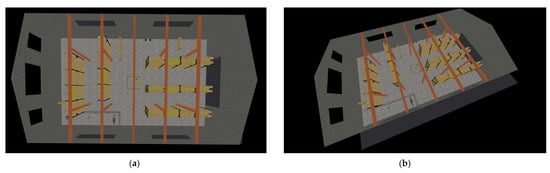
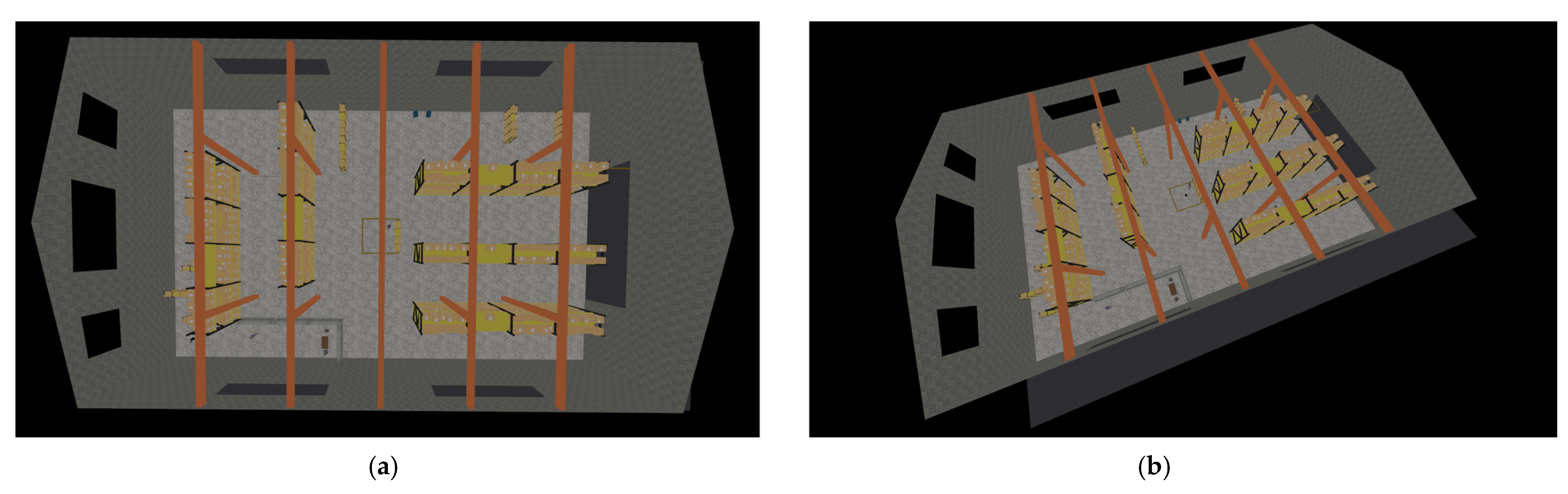
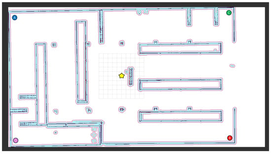
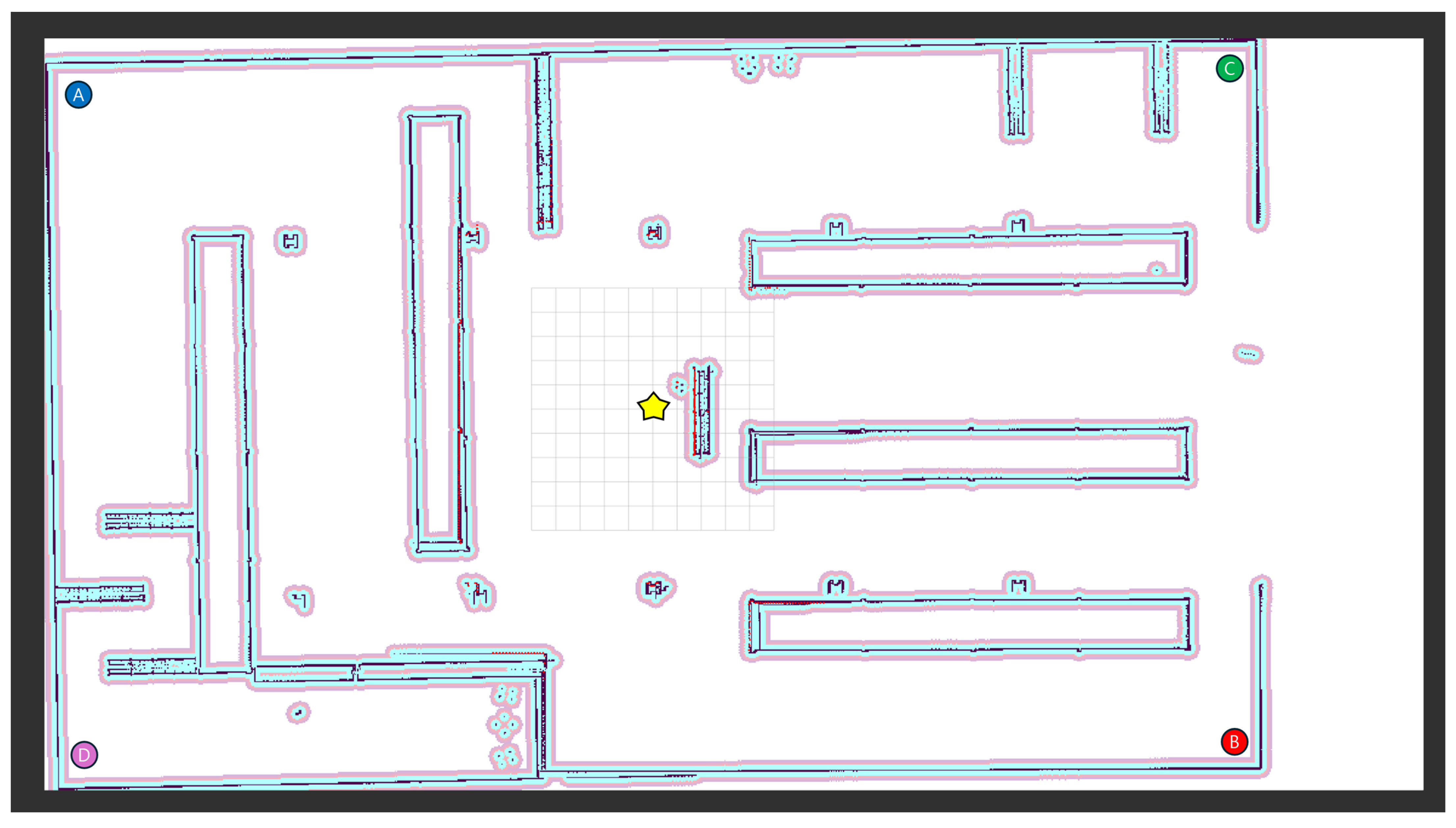
In this section, we conduct a performance evaluation for each algorithm in a warehouse environment as shown in Figure 2. The size of the warehouse is 31.0 m × 56.9 m, and the start point is the yellow star in Figure 3. From the start point, each algorithm performs path planning to a total of four goal positions. The four goal positions correspond to Case $c_1$, Case $c_2$, Case $c_3$ and Case $c_4$. Case $c_1$ refers to path planning from the start position to Position A. Case $c_2$ refers to path planning from the start position to Position B. Case $c_3$ refers to path planning from the start position to Position C. Case $c_4$ refers to path planning from the start position to Position D.

Figure 2. Warehouse simulation environment using the Gazebo simulator. (a) The top-down view. (b) The side view.

Figure 3. Map of the warehouse where the experiments were conducted. The yellow star is the start position. Each algorithm performs path planning toward four goal positions, A, B, C and D. Each position (A, B, C, D) is the goal position for each Case ($c_1$, c₂, c₃, c₄).

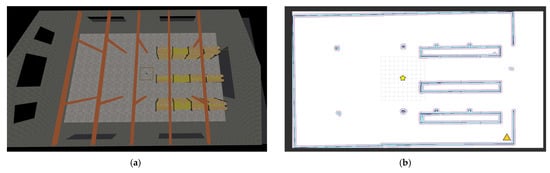
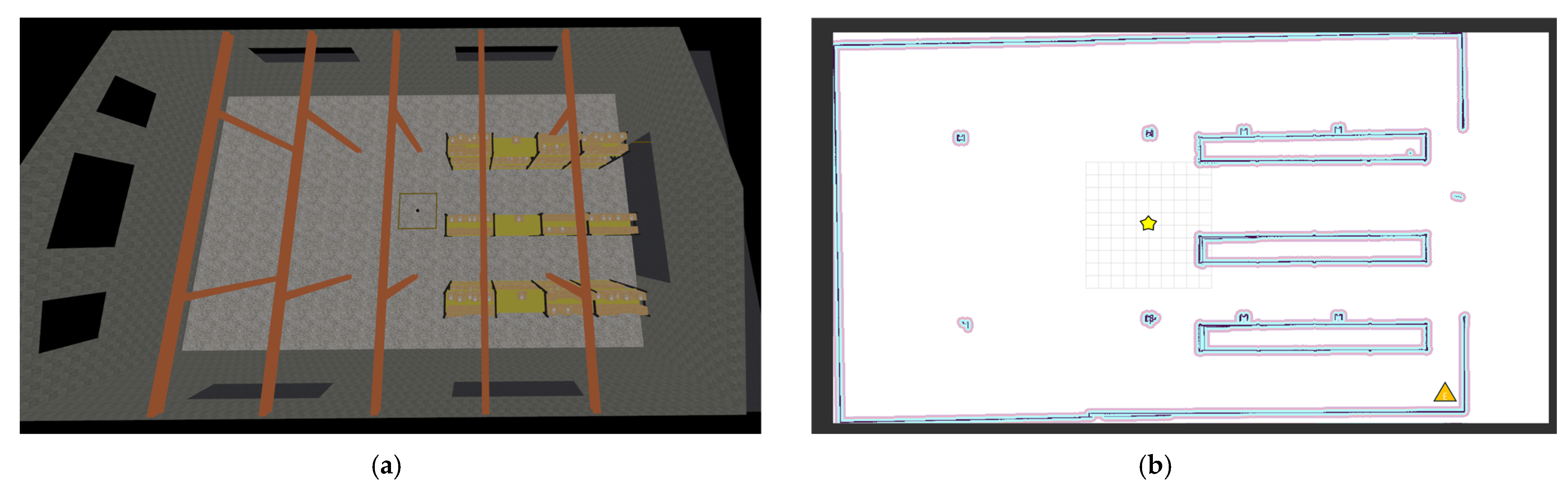
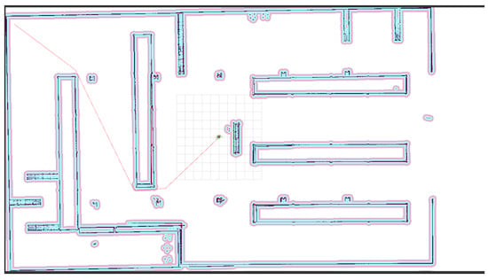
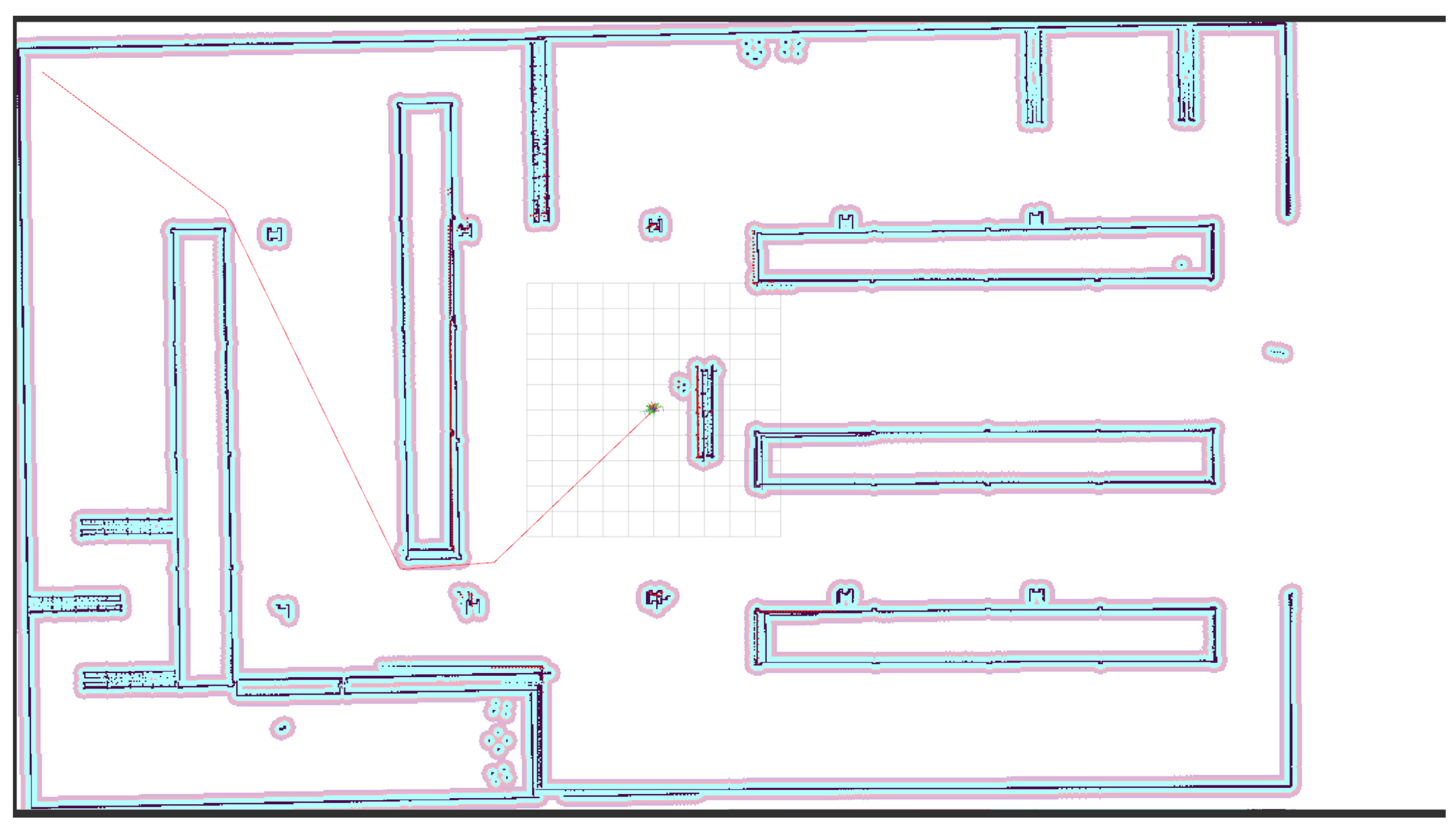
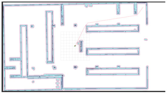
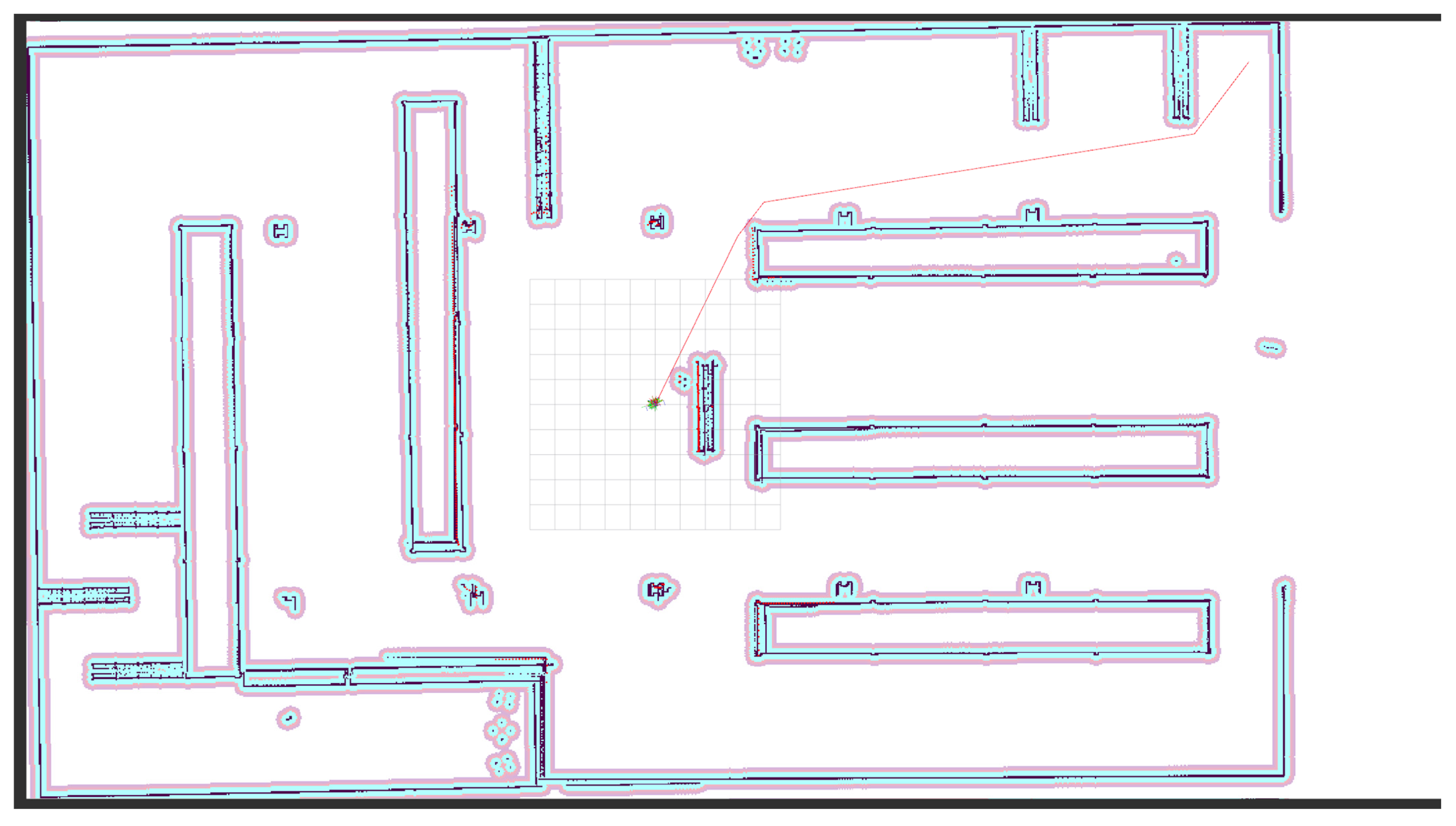
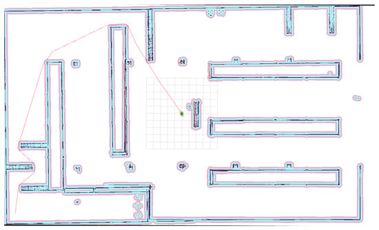
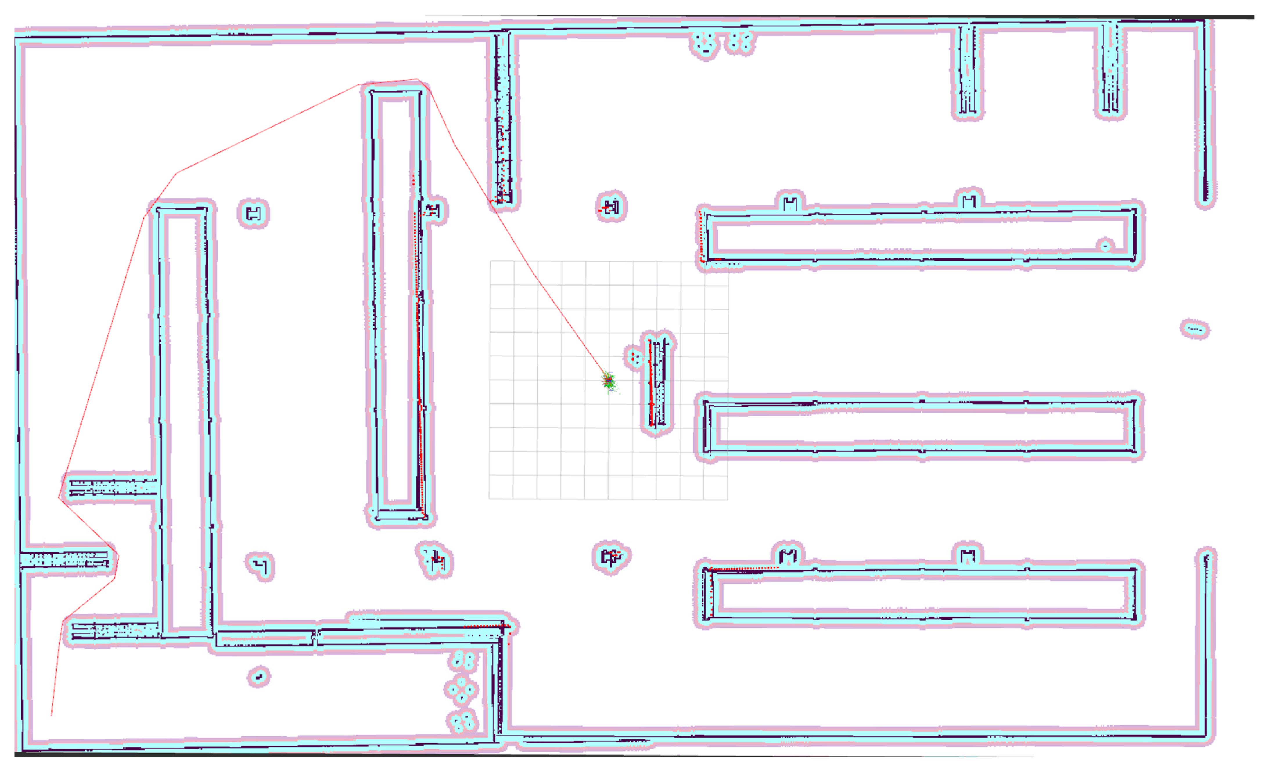
Additionally, a simulation was conducted in an environment containing only three long racks. The environment and map are shown in Figure 4. This environment assumes a warehouse that is much simpler than the maps used in Cases $c_1$–$c_4$. In this map, Case $c_5$ was simulated, where the yellow star shown in Figure 4 indicates the start position. The goal position is marked by an orange triangle. Figure 5, Figure 6 and Figure 7 show the paths of F-RRT for Case $c_1$, MQ-RRT for Case $c_3$, and Q-RRT* for Case $c_4$, respectively.

Figure 4. A simple warehouse environment. (a) A top-down view of the simple warehouse environment. (b) A map of the simple warehouse environment. The yellow star indicates the start position, and the orange triangle indicates the goal position.

Figure 5. Visualization of the optimal path of F-RRT* for Case $c_1$. The red line represents the computed path.

Figure 6. Visualization of the optimal path of MQ-RRT* for Case $c_3$. The red line represents the computed path.

Figure 7. Visualization of the optimal path of Q-RRT* for Case $c_4$. The red line represents the computed path.

4.1. Experimental Setup

The hardware used for the experiments is shown in Table 1. The experimental environment was run on Ubuntu 22.04 Jammy. The simulator used for the simulation was the Gazebo simulator. The version was Harmonic. For the simulation we used ROS2 Humble. Each ROS2 package was implemented in C++.

Table 1. Experimental environment.

Hardware	Specification
CPU	AMD Ryzen 7 9700x 8-core processor
RAM	64.0 GB
VGA	NVIDIA GeForce RTX 5070 Ti

For the experiments parameter values other than $r_{near}$ were defined as follows. In Q-RRT* $D_{ancestry}$ was set to the recommended value of 2. In F-RRT* $D_{ancestry}$ was also set to 2. $D_{dichotomy}$ was set to the recommended value of 2. In MQ-RRT* $D_{ancestry}$ was also set to 2. $D_{dichotomy}$ was set to 2. $R_{commit}$ was set to 1.

For comparative experiments in the warehouse environment the performance evaluation metrics were length of path, planning time and cumulative turning angle. The length of path is the length of the path calculated by each algorithm. Planning time is the time taken by each algorithm to plan a path from the start position to the goal position. The cumulative turning angle can determine how curved the path is. The three evaluation metrics mean better performance when the values are lower. For the experiments, $r_{near}$ was set to 1, 5, 10, 20 and 30. Each algorithm was repeatedly executed 50 times. The time limit for all algorithms was set to 60,000 ms.

The experimental results of the algorithms for each case are presented as the average values over 50 repeated runs. In addition, the three evaluation metrics are presented in normalized form. As shown in Equation (3), the normalization was performed using the case where $r_{near}$ = 1 as the reference.

$$\mathrm{N}\mathrm{o}\mathrm{r}\mathrm{m}\mathrm{a}\mathrm{l}\mathrm{i}\mathrm{z}\mathrm{e}\mathrm{d}={\displaystyle \frac{\mathrm{m}\mathrm{e}\mathrm{a}\mathrm{n}\left(\mathrm{R}\mathrm{e}\mathrm{s}\mathrm{u}\mathrm{l}{\mathrm{t}}_{0\mathrm{t}\mathrm{h}\mathrm{e}\mathrm{r}\mathrm{s}}\right)}{\mathrm{m}\mathrm{e}\mathrm{a}\mathrm{n}\left(\mathrm{R}\mathrm{e}\mathrm{s}\mathrm{u}\mathrm{l}{\mathrm{t}}_{r_{near=1}}\right)}}\times 100$$

(3)

4.2. Experimental Results for Case $c_1$

Table 2 shows the results of comparing the performance of Q-RRT*, F-RRT*, and MQ-RRT* when the neighbor radius parameter $r_{near}$ was changed to 1, 5, 10, 20, and 30 in the Case $c_1$ environment. All values are the mean of 50 repeated runs. Overall, as $r_{near}$ increased, the planning time tended to increase for all three algorithms.

Table 2. Experimental results for Case $c_1$ for each algorithm according to $r_{near}$. The success rate represents the proportion of runs, out of 50 repeated trials, in which a path was computed within 60,000 ms. Each evaluation metric represents the average over the successful runs. The best value in each row is shown in bold.

	${\mathit{r}}_{\mathit{n}\mathit{e}\mathit{a}\mathit{r}}$	1	5	10	20	30
Q-RRT*	Success rate (%)	100	100	100	100	100
	Planning time (ms)	36.3582	59.9204	178.2568	612.8099	1123.745
	Length of Path (m)	44.1	35.5	35.0	34.4	34.5
	Cumulative turning angle (deg)	680.2	124.3	127.5	115.1	118.2
F-RRT*	Success rate (%)	100	100	100	100	100
	Planning time (ms)	15.6501	25.7238	83.2752	153.1248	221.3976
	Length of Path (m)	41.5	39.3	38.6	39.6	39.2
	Cumulative turning angle (deg)	185.0	170.7	164.0	166.3	167.9
MQ-RRT*	Success rate (%)	100	100	100	100	100
	Planning time (ms)	15.001	25.902	60.566	350.293	677.579
	Length of Path (m)	44.006	35.354	34.402	34.526	34.678
	Cumulative turning angle (deg)	778.608	127.664	117.292	124.842	119.016

In contrast, the path quality metrics length of path and cumulative turning angle improved up to a certain range. After that, no significant improvement was observed.

First, for Q-RRT*, the planning time was the fastest at 36.3582 ms when $r_{near}$ = 1. However, under the same condition, the generated path had a length of 44.1 m and a cumulative turning angle of 680.2°. This showed the lowest path quality. When $r_{near}$ was increased to 5, the planning time increased to 59.9204 ms. At the same time, the path length greatly decreased to 35.5 m and the cumulative turning angle also sharply decreased to 124.3°. This confirmed that the path quality improved. For larger $r_{near}$ values, the planning time increased while the improvement in path quality was not large. As shown in Table 3, for Q-RRT*, when $r_{near}$ increased to 10, the normalized planning time became nearly four times higher than that at $r_{near}$ = 1. In contrast, when $r_{near}$ = 5, although the planning time also increased, the path quality improved. In particular, the normalized value of the cumulative turning angle was greatly reduced to 18.28. Accordingly, the heuristically chosen $r_{near}$ value for Q-RRT* was set to 5. In addition, although the path quality improved for the remaining values, they were excluded from the candidate values because the normalized planning time increased by more than four times.

Table 3. Experimental results for Case $c_1$ for each algorithm according to $r_{near}$. The rows excluding the score row present values normalized based on $r_{near}$ = 1.

	${\mathit{r}}_{\mathit{n}\mathit{e}\mathit{a}\mathit{r}}$	1	5	10	20	30
Q-RRT*	Planning time (%)	100	164.81	490.28	1685.48	3090.76
	Length of Path (%)	100	80.52	79.43	78.02	78.33
	Cumulative turning angle (%)	100	18.28	18.75	16.93	17.39
F-RRT*	Planning time (%)	100	164.37	532.11	978.43	1414.67
	Length of Path (%)	100	94.73	93.15	95.60	94.44
	Cumulative turning angle (%)	100	92.31	88.68	89.90	90.79
MQ-RRT*	Planning time (%)	100	172.67	403.75	2335.12	4516.88
	Length of Path (%)	100	80.34	78.18	78.46	78.80
	Cumulative turning angle (%)	100	16.40	15.06	16.03	15.29

Next, for F-RRT*, the planning time was the fastest at 15.6501 ms when $r_{near}$ = 1. However, the generated path had a length of 41.5 m and a cumulative turning angle of 185.0°. This indicated that improvement was needed in terms of path quality. When $r_{near}$ was increased to 5, the planning time increased to 25.7238 ms, but the path length decreased to 39.3 m and the cumulative turning angle also decreased to 170.7°. This confirmed that the path quality improved. After that, at $r_{near}$ = 10, the planning time increased to 83.2752 ms, while the path length was 38.6 m and the cumulative turning angle was 164.0°. This showed the best path quality. When $r_{near}$ was further increased to 20 and 30, the planning time continued to increase to 153.1248 ms and 221.3976 ms. In contrast, the path length at 39.6 m and 39.2 m and the cumulative turning angle at 166.3° and 167.9° did not show quality improvement compared to $r_{near}$ = 10. As shown in Table 3, the normalized planning time values increased by more than five times when $r_{near}$ =10, 20, and 30. This indicates that, although the normalized values of the length of path and cumulative turning angle improved to below 100, the increase in planning time was substantial. In contrast, when $r_{near}$ = 5, only a slight increase in planning time was observed, while the path quality improved. Therefore, $r_{near}$ = 5 was selected as the heuristically chosen value.

For MQ-RRT*, the planning time was the fastest at 15.001 ms when $r_{near}$ = 1. As with the previous algorithms, it showed the lowest tendency in path quality. When $r_{near}$ was increased to 5, the planning time increased to 25.902 ms. In contrast, the path length decreased to 35.354 m and the cumulative turning angle sharply decreased to 127.664°. This confirmed a clear improvement in path quality. After that, at $r_{near}$ = 10, the planning time increased to 60.566 ms, but the path length became shorter to 34.402 m and the cumulative turning angle further decreased to 117.292°. The quality improved once more. However, when $r_{near}$ was increased to 20 and 30, the planning time increased greatly to 350.293 ms and 677.579 ms. Therefore, in Case $c_1$, $r_{near}$ = 5 was selected based on heuristically observations, as the planning time increased only slightly while the path quality improved substantially.

4.3. Experimental Results for Case $c_2$

Table 4 shows the results of comparing the performance of Q-RRT*, F-RRT*, and MQ-RRT* when the neighbor radius parameter $r_{near}$ was changed to 1, 5, 10, 20, and 30 in the Case $c_2$ environment.

Table 4. Experimental results for Case $c_2$ for each algorithm according to $r_{near}$. The success rate represents the proportion of runs, out of 50 repeated trials, in which a path was computed within 60,000 ms. Each evaluation metric represents the average over the successful runs. The best value in each row is shown in bold.

	${\mathit{r}}_{\mathit{n}\mathit{e}\mathit{a}\mathit{r}}$	1	5	10	20	30
Q-RRT*	Success rate (%)	100	100	100	100	100
	Planning time (ms)	207.398	212.3625	711.6966	289.9497	380.7755
	Length of Path (m)	37.8	32.6	33.6	31.1	30.9
	Cumulative turning angle (deg)	578.6	127.3	129.8	119.1	118.5
F-RRT*	Success rate (%)	100	100	100	100	100
	Planning time (ms)	31.4709	103.0863	26.001	35.0317	24.7851
	Length of Path (m)	37.4	35.6	36.6	35.3	34.6
	Cumulative turning angle (deg)	120.9	101.7	102.2	109.8	103.4
MQ-RRT*	Success rate (%)	100	100	100	100	100
	Planning time (ms)	22.946	34.334	97.125	536.863	1705.039
	Length of Path (m)	38.118	33.028	31.904	31.372	30.944
	Cumulative turning angle (deg)	676.554	128.992	124.096	123.666	120.548

For Q-RRT*, the planning time was the fastest at 207.398 ms when $r_{near}$ = 1. However, the path quality tended to be the lowest. When $r_{near}$ was increased to 5, the planning time increased slightly to 212.3625 ms. In contrast, the path length decreased to 32.6 m and the cumulative turning angle sharply decreased to 127.3°. This confirmed that the path quality clearly improved. However, at $r_{near}$ = 10, the planning time greatly increased to 711.6966 ms. At the same time, the path length of 33.6 m and the cumulative turning angle of 129.8° became worse compared to $r_{near}$ = 5. This range appeared to be inefficient in both time and quality. It can be observed that when $r_{near}$ = 20 and 30, the path was computed faster than when $r_{near}$ = 10. The path quality was the best when $r_{near}$ = 30, followed by $r_{near}$ = 20. As shown in Table 5, excluding $r_{near}$ = 10 and 30, which had high normalized planning time values, the value that showed the best path quality among the remaining candidates was 20. Therefore, $r_{near}$ = 20 was selected as the heuristically chosen value.

Table 5. Experimental results for Case $c_2$ for each algorithm according to $r_{near}$. The rows excluding the score row present values normalized based on $r_{near}$ = 1.

	${\mathit{r}}_{\mathit{n}\mathit{e}\mathit{a}\mathit{r}}$	1	5	10	20	30
Q-RRT*	Planning time (%)	100	102.39	343.15	139.80	183.60
	Length of Path (%)	100	86.33	88.74	82.23	81.81
	Cumulative turning angle (%)	100	22.01	22.43	20.59	20.49
F-RRT*	Planning time (%)	100	327.56	82.62	111.31	78.76
	Length of Path (%)	100	95.24	97.85	94.44	92.53
	Cumulative turning angle (%)	100	84.14	84.52	90.77	85.48
MQ-RRT*	Planning time (%)	100	149.63	423.27	2339.67	7430.63
	Length of Path (%)	100	86.65	83.70	82.30	81.18
	Cumulative turning angle (%)	100	19.07	18.34	18.28	17.82

For F-RRT*, the planning time was 31.4709 ms when $r_{near}$ = 1. The path length was 37.4 m and the cumulative turning angle was 120.9°. When $r_{near}$ was increased to 5, the path length decreased to 35.6 m and the cumulative turning angle decreased to 101.7°, which was the lowest value. This showed an advantage in terms of quality, but the planning time greatly increased to 103.0863 ms. After that, at $r_{near}$ = 10, the planning time decreased again to 26.001 ms and the cumulative turning angle was 102.2°. However, the path length increased to 36.6 m compared to $r_{near}$ = 5 and 20 and 30. At $r_{near}$ = 20, the path length improved to 35.3 m, but the cumulative turning angle increased to 109.8°. At $r_{near}$ = 30, the planning time was the shortest at 24.7851 ms and the path length was also the shortest at 34.6 m. The cumulative turning angle was also maintained at a sufficiently low level at 103.4°. As shown in Table 5, when $r_{near}$ = 30, the normalized values of planning time and length of path were the lowest. In addition, compared with the best result for the cumulative turning angle, the difference was only 1.34, indicating only a slightly greater amount of turning. Accordingly, in Case $c_2$, $r_{near}$ = 30 was set as the heuristically chosen value for F-RRT*.

For MQ-RRT*, the planning time was relatively fast at 22.946 ms when $r_{near}$ = 1, but the path length was the longest at 38.118 m and the cumulative turning angle was 676.554°, which showed the lowest quality. When $r_{near}$ was increased to 5, the planning time became the shortest at 34.334 ms. The path length decreased to 33.028 m and the cumulative turning angle also decreased to 128.992°. This confirmed that the path quality improved. However, at $r_{near}$ = 10, the planning time increased to 97.125 ms, and at the same time, the path length of 31.904 m and the cumulative turning angle of 124.096° became improved compared to $r_{near}$ = 5. At $r_{near}$ = 20, the planning time increased further to 536.863 ms, while the quality did not improve much. At $r_{near}$ = 30, the path length of 30.944 m and the cumulative turning angle of 120.548° showed the best quality, but the planning time increased to 1705.039 ms. This showed a tendency that the time cost became much larger compared to $r_{near}$ = 5. Therefore, in Case $c_2$, $r_{near}$ = 5 was selected as the heuristically chosen value for MQ-RRT*.

4.4. Experimental Results for Case $c_3$

Table 6 shows the results of comparing the performance of Q-RRT*, F-RRT*, and MQ-RRT* when the neighbor radius parameter $r_{near}$ was changed to 1, 5, 10, 20, and 30 in the Case $c_3$ environment.

Table 6. Experimental results for Case $c_3$ for each algorithm according to $r_{near}$. The success rate represents the proportion of runs, out of 50 repeated trials, in which a path was computed within 60,000 ms. Each evaluation metric represents the average over the successful runs. The best value in each row is shown in bold.

	${\mathit{r}}_{\mathit{n}\mathit{e}\mathit{a}\mathit{r}}$	1	5	10	20	30
Q-RRT*	Success rate (%)	100	100	100	100	100
	Planning time (ms)	198.5187	321.0299	498.9848	398.8026	418.7209
	Length of Path (m)	40.5	34.3	33.7	31.766	31.9
	Cumulative turning angle (deg)	593.9	129.8	128.9	129.8	133.4
F-RRT*	Success rate (%)	100	100	100	100	100
	Planning time (ms)	103.4510	133.9447	96.4212	42.9048	119.8214
	Length of Path (m)	41.9	36.4	36.7	37.1	35.1
	Cumulative turning angle (deg)	180.9	148.7	148.6	152.9	148.7
MQ-RRT*	Success rate (%)	100	100	100	100	100
	Planning time (ms)	23.703	24.979	81.644	643.231	1304.182
	Length of Path (m)	43.278	34.908	34.044	32.448	31.7
	Cumulative turning angle (deg)	745.092	144.626	139.15	139.502	138.824

For Q-RRT*, the planning time was the fastest at 198.5187 ms when $r_{near}$ = 1. However, as in Cases $c_1$ and $c_2$, $r_{near}$ = 1 was fast but the path quality was the worst. In particular, as shown in Table 7, the normalized values of the cumulative turning angle were in the low 20% range when $r_{near}$ = 5, 10, 20, and 30. For Q-RRT*, when $r_{near}$ was increased to 5, the planning time increased to 321.0299 ms. The path length decreased to 34.3 m. The cumulative turning angle also decreased to 129.8°. The path quality improved. In the later values, the planning time increased. The improvement in path length was not large. At $r_{near}$ = 10, the planning time increased further to 498.9848 ms. The improvement in path length to 33.7 m was not large. The cumulative turning angle decreased only slightly to 128.9°. At $r_{near}$ = 20, the path length became the shortest at 31.766 m. The planning time was 398.8026 ms. The cumulative turning angle was 129.82°. It increased compared to $r_{near}$ = 10. At $r_{near}$ = 30, the planning time increased to 418.7209 ms. No further path-quality improvement was observed compared to $r_{near}$ = 20. Therefore, in Case $c_3$, $r_{\mathrm{near}}=20$ was selected as the heuristically chosen value for Q-RRT*. The path length was the shortest. The cumulative turning angle was the second lowest.

Table 7. Experimental results for Case $c_3$ for each algorithm according to $r_{near}$. The rows excluding the score row present values normalized based on $r_{near}$ = 1.

	${\mathit{r}}_{\mathit{n}\mathit{e}\mathit{a}\mathit{r}}$	1	5	10	20	30
Q-RRT*	Planning time (%)	100	161.71	251.35	200.89	210.92
	Length of Path (%)	100	84.51	83.16	78.27	78.60
	Cumulative turning angle (%)	100	21.86	21.71	21.86	22.47
F-RRT*	Planning time (%)	100	129.48	93.20	41.47	115.82
	Length of Path (%)	100	86.98	87.67	88.60	83.99
	Cumulative turning angle (%)	100	82.17	82.21	84.51	82.21
MQ-RRT*	Planning time (%)	100	105.38	344.44	2713.61	5501.98
	Length of Path (%)	100	80.66	78.66	74.98	73.25
	Cumulative turning angle (%)	100	19.41	18.68	18.72	18.63

For F-RRT*, the planning time was 103.451 ms when $r_{near}$ = 1. The path length was 41.9 m. The cumulative turning angle was 180.9°. The quality was somewhat low. When $r_{near}$ was increased to 5, the planning time increased to 133.9447 ms. The path length decreased to 36.4 m. The cumulative turning angle decreased to 148.7°. The path quality improved. At $r_{near}$ = 10, the planning time decreased again to 96.4212 ms. The cumulative turning angle was the lowest at 148.6°. However, the path length was 36.7 m. It increased slightly compared to $r_{near}$ = 5. After that, at $r_{near}$ = 20, the planning time was the lowest at 42.9048 ms. The computational efficiency improved greatly. The path length was 37.1 m. It was maintained without large degradation. At $r_{near}$ = 30, the path length became the shortest at 35.1 m. However, the planning time increased greatly to 119.8214 ms. Therefore, in Case $c_3$, $r_{near}$ = 20 was selected as the heuristically chosen value for F-RRT*, as it reduced the planning time the most while maintaining the path quality at an acceptable level.

For MQ-RRT*, the planning time was relatively fast at 23.703 ms when $r_{near}$ = 1. However, the path length was the longest at 43.278 m. The cumulative turning angle was very large at 745.092°. The path quality was the lowest. When $r_{near}$ was increased to 5, the planning time was 24.979 ms. At the same time, the path length greatly decreased to 34.908 m. The cumulative turning angle also decreased to 144.626°. The time and quality both improved. However, when $r_{near}$ = 10, the planning time increased to 81.644 ms. The path length decreased further to 34.044 m compared to $r_{near}$ = 5. In contrast, at $r_{near}$ = 20 and 30, the planning time continued to increase to 643.231 ms and 1304.182 ms. The improvement in path length was not large at 32.448 m and 31.7 m. In addition, the improvement in the cumulative turning angle was not substantial.

As shown in Table 7, when $r_{near}$ = 20 and 30, the normalized planning time values increased by more than ten times. This indicates that the performance deteriorated excessively in terms of speed. When $r_{near}$ = 5, the planning time increased by only 5.38%, whereas the length of path and cumulative turning angle were reduced to 80.66% and 19.41%, respectively, indicating a substantial improvement in path quality. In the case of $r_{near}$ = 10, the planning time was more than three times slower than that of $r_{near}$ = 5. However, the improvement in path quality was not significant in comparison. Therefore, in Case $c_3$, $r_{near}$ = 5 was selected as the heuristically chosen value for MQ-RRT*.

4.5. Experimental Results for Case $c_4$

Table 8 shows the results of comparing the performance of Q-RRT*, F-RRT*, and MQ-RRT* when the neighbor radius parameter $r_{near}$ was changed to 1, 5, 10, 20, and 30 in the Case $c_4$ environment. In Case $c_4$, there were instances in which Q-RRT* and F-RRT* exceeded the given time limit of 60,000 ms. As shown in Table 8, for Q-RRT*, the success rate decreased sharply from $r_{near}$ = 20. Furthermore, when $r_{near}$ = 30, the success rate was 0%. The normalized values are presented in Table 9. In this case, the results with a success rate of 50% or lower were excluded.

Table 8. Experimental results for Case $c_4$ for each algorithm according to $r_{near}$. The success rate represents the proportion of runs, out of 50 repeated trials, in which a path was computed within 60,000 ms. Each evaluation metric represents the average over the successful runs. The best value in each row is shown in bold.

	${\mathit{r}}_{\mathit{n}\mathit{e}\mathit{a}\mathit{r}}$	1	5	10	20	30
Q-RRT*	Success rate (%)	100	100	100	16	0
	Planning time (ms)	1452.99	2479.26	8471.18	44,105.64	-
	Length of Path (m)	61.45	52.25	52.40	52.51	-
	Cumulative turning angle (deg)	763.36	386.92	382.04	369.55	-
F-RRT*	Success rate (%)	100	100	100	22	0
	Planning time (ms)	1749.04	4367.73	15,484.62	41,397.61	-
	Length of Path (m)	62.74	54.51	54.85	54.27	-
	Cumulative turning angle (deg)	555.11	427.24	423.87	407.60	-
MQ-RRT*	Success rate (%)	100	100	100	100	100
	Planning time (ms)	104.00	158.92	515.82	3135.20	8212.23
	Length of Path (m)	70.74	53.20	53.03	53.19	53.35
	Cumulative turning angle (deg)	1526.20	410.13	394.60	397.42	397.87

Table 9. Experimental results for Case $c_4$ for each algorithm according to $r_{near}$. The rows excluding the score row present values normalized based on $r_{near}$ = 1.

	${\mathit{r}}_{\mathit{n}\mathit{e}\mathit{a}\mathit{r}}$	1	5	10	20	30
Q-RRT*	Planning time (%)	100	170.63	583.01	-	-
	Length of Path (%)	100	85.03	85.27	-	-
	Cumulative turning angle (%)	100	50.69	50.05	-	-
F-RRT*	Planning time (%)	100	249.72	885.32	-	-
	Length of Path (%)	100	86.88	87.42	-	-
	Cumulative turning angle (%)	100	76.97	76.36	-	-
MQ-RRT*	Planning time (%)	100	152.80	495.95	3014.38	7895.77
	Length of Path (%)	100	75.21	74.97	75.19	75.42
	Cumulative turning angle (%)	100	26.87	25.86	26.04	26.07

For Q-RRT*, the planning time was the shortest when $r_{near}$ = 1, at 1452.99 ms. However, the length of path was 61.45 and the cumulative turning angle was 763.36, indicating poor path quality. When $r_{near}$ was increased to 5, the path quality improved. In the case of $r_{near}$ = 10, the path quality did not differ significantly from that at $r_{near}$ = 5. As shown in Table 9, when $r_{near}$ = 10, the planning time deteriorated significantly compared with the cases of $r_{near}$ = 1 and 5. When $r_{near}$ = 5, the planning time increased, but the length of path and cumulative turning angle improved to 85.03% and 50.69%, respectively. Therefore, in Case $c_4$, $r_{near}$ = 5 was selected as the heuristically chosen value for Q-RRT*.

For F-RRT*, as in the other cases, the planning time tended to increase as $r_{near}$ increased. However, from $r_{near}$ = 20, the planning time increased sharply, and the success rate reached only 22%. When $r_{\mathrm{near}}$ = 30, the success rate was 0%. When $r_{\mathrm{near}}=5$, the planning time increased to some extent, but the cumulative turning angle improved substantially. Accordingly, in Case $c_4$, $r_{\mathrm{near}}=5$ was selected as the heuristically chosen value for F-RRT*.

For MQ-RRT*, as shown in Table 9, the normalized planning time values for $r_{near}$ = 20 and 30 were 3014.38 and 7895.77, respectively, indicating that they were much slower than the other $r_{near}$ values. In contrast, for the length of path, no substantial difference was observed among the normalized values when $r_{near}$ = 5, 10, 20, and 30. A similar trend was observed for the cumulative turning angle. When $r_{near}$ = 10, 20, and 30, the normalized planning time values were nearly more than five times higher than the reference value at $r_{near}$ = 1. In contrast, when $r_{near}$ = 5, there was a slight trade-off, with the normalized planning time reaching 152.80%, but the path quality showed improvement. Accordingly, in Case $c_4$, $r_{near}$ = 5 was selected as the heuristically chosen value for MQ-RRT*.

4.6. Experimental Results for Case $c_5$

Table 10 shows the results of comparing the performance of Q-RRT*, F-RRT*, and MQ-RRT* when the neighbor radius parameter $r_{near}$ was changed to 1, 5, 10, 20, and 30 in the Case $c_5$ environment. Table 11 shows the normalized results of each performance metric based on $r_{near}$ = 1.

Table 10. Experimental results for Case $c_5$ for each algorithm according to $r_{near}$. The success rate represents the proportion of runs, out of 50 repeated trials, in which a path was computed within 60,000 ms. Each evaluation metric represents the average over the successful runs. The best value in each row is shown in bold.

	${\mathit{r}}_{\mathit{n}\mathit{e}\mathit{a}\mathit{r}}$	1	5	10	20	30
Q-RRT*	Success rate (%)	100	100	100	100	100
	Planning time (ms)	403.39	440.24	981.58	5800.76	5634.72
	Length of Path (m)	39.77	34.43	34.00	32.15	31.63
	Cumulative turning angle (deg)	579.78	92.076	93.81	99.14	109.68
F-RRT*	Success rate (%)	100	100	100	100	100
	Planning time (ms)	138.72	522.03	1644.74	4942.61	6106.12
	Length of Path (m)	36.534	35.866	34.088	35.258	35.82
	Cumulative turning angle (deg)	91.68	94.584	83.58	91.088	90.71
MQ-RRT*	Success rate (%)	100	100	100	100	100
	Planning time (ms)	20.44	20.87	113.04	678.78	1326.82
	Length of Path (m)	40.66	34.18	33.438	31.906	31.724
	Cumulative turning angle (deg)	658.966	92.244	93.476	98.002	107.084

Table 11. Experimental results for Case $c_5$ for each algorithm according to $r_{near}$. The rows excluding the score row present values normalized based on $r_{near}$ = 1.

	${\mathit{r}}_{\mathit{n}\mathit{e}\mathit{a}\mathit{r}}$	1	5	10	20	30
Q-RRT*	Planning time (%)	100	109.14	243.33	1438.00	1396.84
	Length of Path (%)	100	86.58	85.49	80.84	79.54
	Cumulative turning angle (%)	100	15.88	16.18	17.10	18.92
F-RRT*	Planning time (%)	100	376.32	1185.65	3562.98	4401.72
	Length of Path (%)	100	98.17	93.30	96.51	98.05
	Cumulative turning angle (%)	100	103.17	91.16	99.35	98.94
MQ-RRT*	Planning time (%)	100	102.14	553.03	3320.59	6490.74
	Length of Path (%)	100	84.06	82.24	78.47	78.02
	Cumulative turning angle (%)	100	14.00	14.19	14.87	16.25

In the case of Q-RRT, when $r_{near}$ = 1, the planning time was the fastest at 403.39 ms. However, the path length was the longest at 39.77 m, and the cumulative turning angle was very large at 579.78°, indicating that the path quality was the lowest. When $r_{near}$ was increased to 5, the planning time increased to 440.24 ms, but the path length decreased to 34.43 m and the cumulative turning angle also decreased to 92.076°. This shows that when $r_{near}$ was increased from 1 to 5, the path quality improved significantly. Table 11 also shows that when $r_{near}$ = 5, the planning time increased by only 9.14% to 109.14% of the baseline, whereas the path length and cumulative turning angle decreased to 86.58% and 15.88%, respectively. After that, at $r_{near}$ = 10, the planning time increased further to 981.58 ms, but the path length decreased only slightly to 34.00 m, and the cumulative turning angle rather increased slightly to 93.81° compared to $r_{near}$ = 5. At $r_{near}$ = 20, the path length became shorter at 32.15 m, but the planning time increased greatly to 5800.76 ms, and the cumulative turning angle also increased again to 99.14°. At $r_{near}$ = 30, the path length was the shortest at 31.63 m, but the planning time was very large at 5634.72 ms, and the cumulative turning angle further worsened to 109.68°. Therefore, in Case $c_5$, for Q-RRT, $r_{near}$ = 5 is considered to be a value that significantly improved the path quality with only a very small increase in time, and it is reasonable to regard it as the heuristically chosen value.

In the case of F-RRT, at $r_{near}$ = 1, the planning time was the fastest at 138.72 ms, the path length was 36.534 m, and the cumulative turning angle was 91.68°. When $r_{near}$ was increased to 5, the planning time increased to 522.03 ms, but the path length showed only a slight decrease to 35.866 m. In addition, the cumulative turning angle increased to 94.584°. At $r_{near}$ = 10, the path length was the shortest at 34.088 m, and the cumulative turning angle was also the lowest at 83.58°, showing the best result in terms of path quality. However, the planning time increased greatly to 1644.74 ms. As shown in Table 11, at $r_{near}$ = 10, the path length and cumulative turning angle improved to 93.30% and 91.16%, respectively, but the planning time increased very greatly to 1185.65%. After that, at $r_{near}$ = 20 and 30, the planning time increased to 4942.61 ms and 6106.12 ms, respectively, but the path length and cumulative turning angle rather did not improve compared to $r_{near}$ = 10. In F-RRT, as $r_{near}$ increased, the increase in computation time was very large, whereas the improvement in path quality was limited or inconsistent. Therefore, in Case $c_5$, for F-RRT*, it is considered appropriate to heuristically choose $r_{near}$ = 1, which showed the highest computational efficiency while the path quality was not very poor.

In the case of MQ-RRT, at $r_{near}$ = 1, the planning time was the fastest at 20.44 ms, but the path length was the longest at 40.66 m and the cumulative turning angle was very large at 658.966°, indicating that the path quality was the lowest. At $r_{near}$ = 5, although the planning time hardly increased and was 20.87 ms, the path length greatly decreased to 34.18 m and the cumulative turning angle also sharply decreased to 92.244°, so the path quality improved significantly. Table 11 also shows that when $r_{near}$ = 5, the planning time increased by only 2.14% to 102.14% of the baseline, whereas the path length and cumulative turning angle decreased to 84.06% and 14.00%, respectively, confirming that improvement was achieved. At $r_{near}$ = 10, the planning time increased to 113.04 ms, and the path length decreased slightly further to 33.438 m, but the cumulative turning angle rather increased to 93.476° compared to $r_{near}$ = 5. In addition, Table 11 shows that the planning time increased greatly to 553.03%, whereas the improvement in path quality was relatively not large. After that, at $r_{near}$ = 20 and 30, the planning time increased greatly to 678.78 ms and 1326.82 ms, respectively, and the path length became somewhat shorter at 31.906 m and 31.724 m, but the cumulative turning angle increased again to 98.002° and 107.084°. This means that the improvement in quality was limited compared to the large increase in time. Therefore, in Case $c_5$, for MQ-RRT, $r_{near}$ = 5 is considered to be the heuristically chosen value because it significantly improved the path quality with almost the same computation time as $r_{near}$ = 1.

Overall, in Case $c_5$, in both Q-RRT and MQ-RRT, a small increase in $r_{near}$ greatly improved the path quality, whereas an excessively large $r_{near}$ rapidly increased the planning time and was inefficient. On the other hand, in F-RRT, the gain from increasing $r_{near}$ was relatively small and the increase in computation time was large, so the default value $r_{near}$ = 1 was heuristically chosen. Therefore, in Case $c_5$, $r_{near}$ = 5 was heuristically chosen for Q-RRT and MQ-RRT, and $r_{near}$ = 1 was heuristically chosen for F-RRT.

4.7. Performance Comparison of Each Algorithm Using the Heuristically Chosen $r_{near}$

In this section, we perform a comparison using the heuristically chosen $r_{near}$ value of each algorithm. Based on Section 4.2, Section 4.3, Section 4.4, Section 4.5 and Section 4.6, the heuristically chosen $r_{near}$ values selected for each case are shown in Table 12.

Table 12. The heuristically chosen $r_{near}$ values of each algorithm for each case.

	$\mathbf{Case} {\mathit{c}}_1$	$\mathbf{Case} {\mathit{c}}_2$	$\mathbf{Case} {\mathit{c}}_3$	$\mathbf{Case} {\mathit{c}}_4$	$\mathbf{Case} {\mathit{c}}_5$
Q-RRT*	5	20	20	5	5
F-RRT*	5	30	20	5	1
MQ-RRT*	5	5	5	5	5

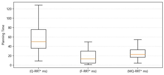
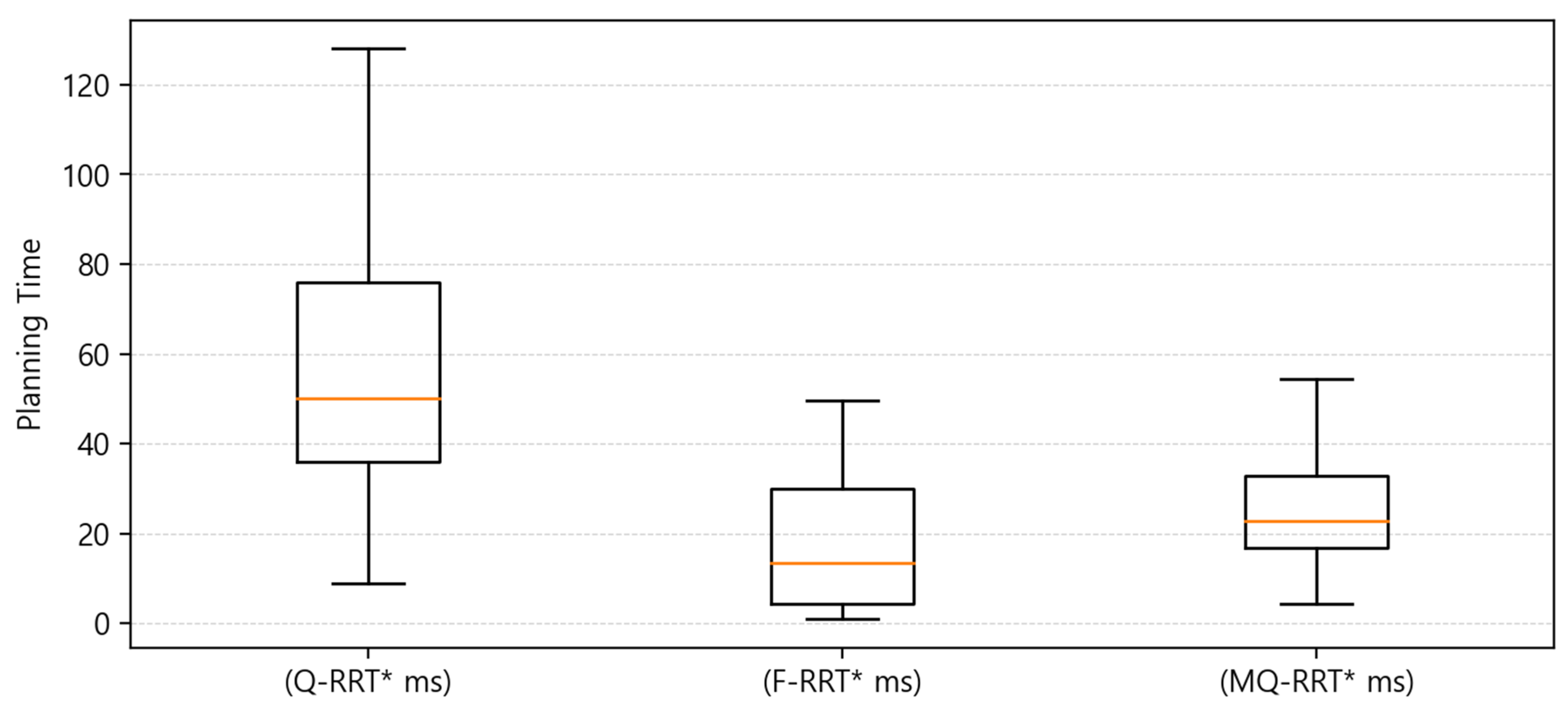
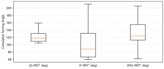
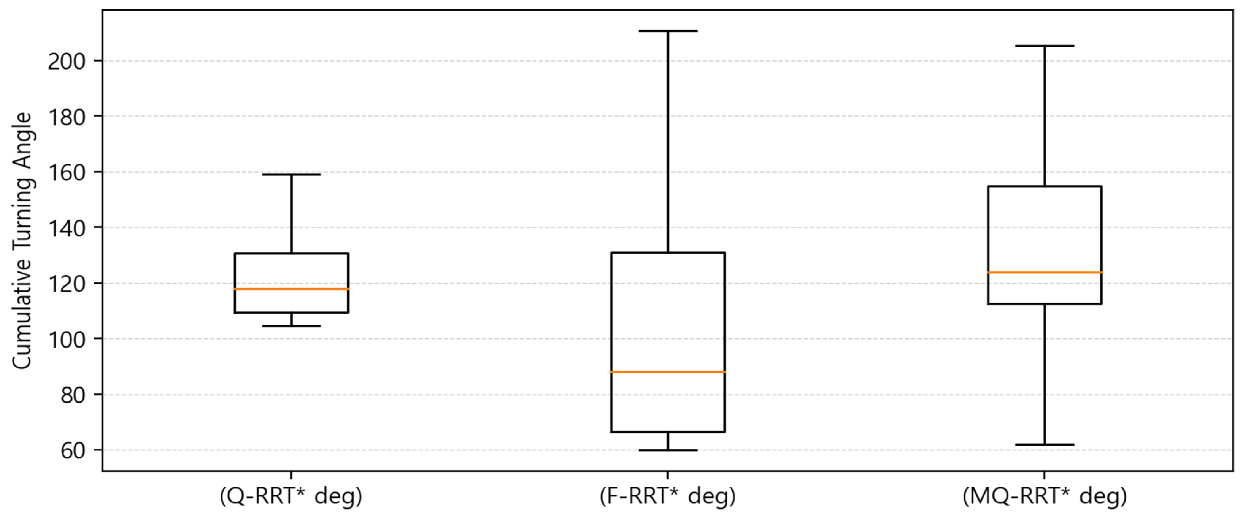
In Case $c_1$, the performance of Q-RRT*, F-RRT*, and MQ-RRT* was compared in terms of planning time, length of path, and cumulative turning angle. From the box plot analysis, the three algorithms showed different characteristics in terms of computational efficiency and path quality.

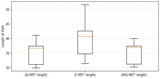
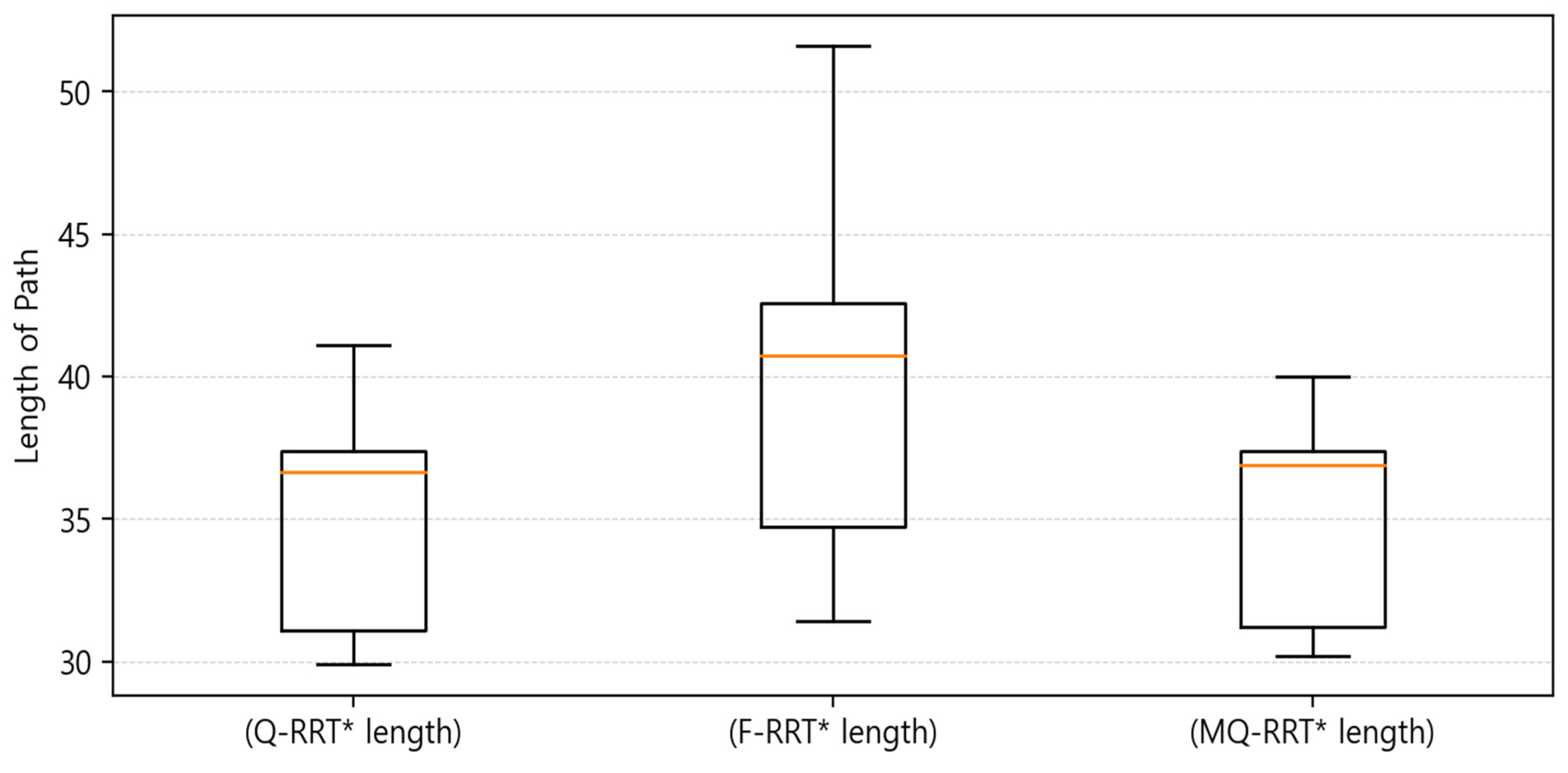
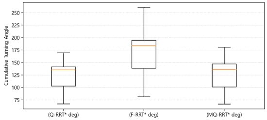
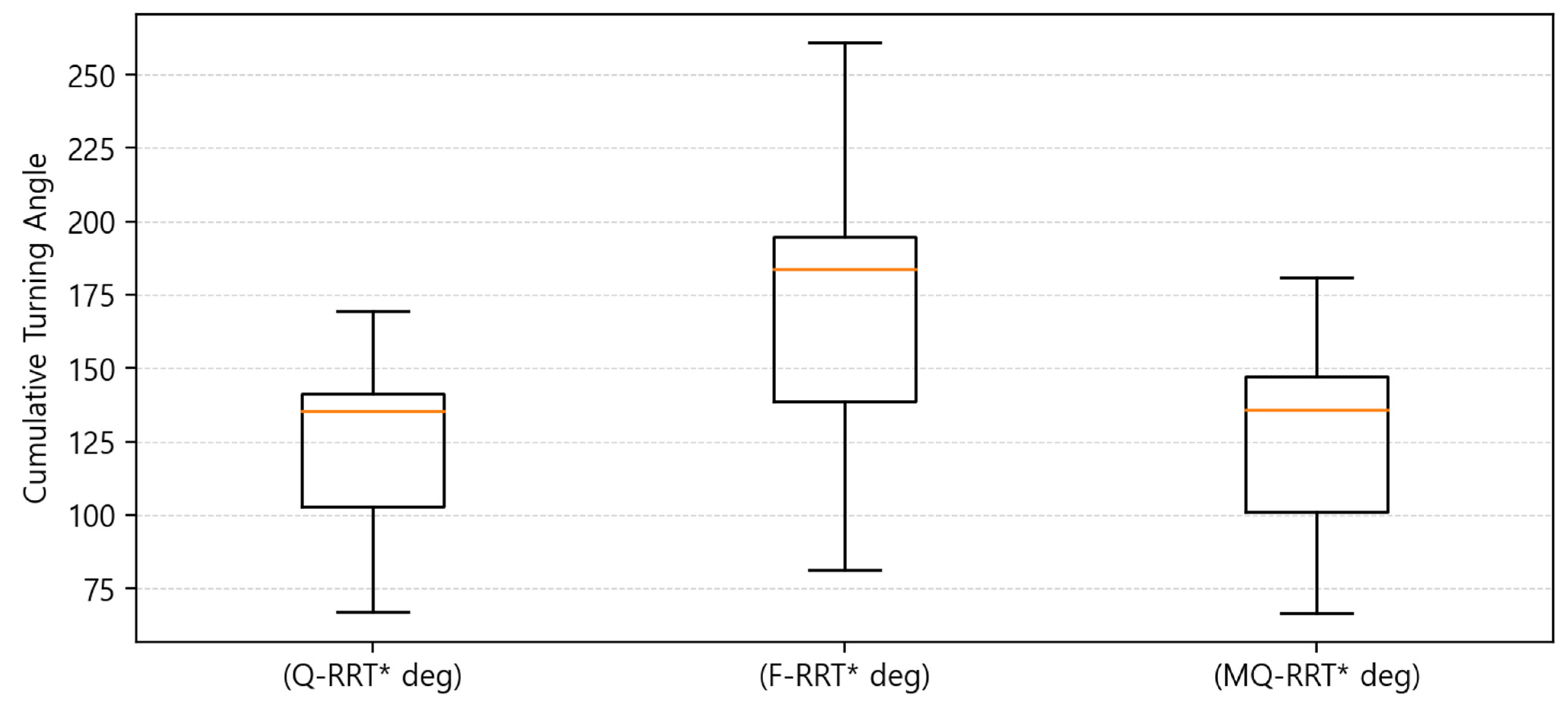
Figure 8 shows that F-RRT* exhibited the fastest performance in terms of planning time. In addition, as shown in Table 13, F-RRT* had the lowest median value. In contrast, although MQ-RRT* was slower than F-RRT*, it showed the highest consistency in planning time because it had the smallest interquartile range (IQR) and standard deviation. Q-RRT* had the largest median value, and its computation time showed the greatest variation in terms of the interquartile range. As shown in Figure 9, in terms of path length, Q-RRT* generally generated the shortest path. MQ-RRT* had a median similar to that of Q-RRT*, but the computed path was slightly longer. However, MQ-RRT* had the narrowest interquartile range, indicating the highest consistency. F-RRT* showed the longest path in terms of the median value. It also had the largest interquartile range, indicating the lowest consistency. This shows that, in the Case $c_1$ environment, F-RRT* was inferior to the other algorithms in terms of path efficiency. As shown in Figure 10, Q-RRT* had the lowest median value for the cumulative turning angle. MQ-RRT* had a slightly higher median than Q-RRT*, but a lower one than F-RRT*. F-RRT* had a high median value and also the largest interquartile range.

Figure 8. Box plot of the planning time results for Case $c_1$.

Table 13. Summary of the experimental results for Case $c_1$ (quartiles and standard deviation).

		Q1	Q2	Q3	IQR	Std.
Planning time (ms)	Q-RRT*	35.89	50.16	75.88	39.99	37.74
	F-RRT*	4.44	13.32	29.88	25.44	36.01
	MQ-RRT*	16.84	22.70	32.70	15.86	13.96
Length of Path (m)	Q-RRT*	31.10	36.65	37.37	6.27	3.35
	F-RRT*	34.72	40.75	42.57	7.85	4.87
	MQ-RRT*	31.22	36.90	37.40	6.17	3.09
Cumulative turning angle (deg)	Q-RRT*	102.80	135.55	141.45	38.65	27.31
	F-RRT*	138.87	183.80	194.77	55.90	46.04
	MQ-RRT*	101.05	135.75	147.07	46.02	30.70

Figure 9. Box plot of the length of path results for Case $c_1$.

Figure 10. Box plot of the cumulative turning angle results for Case $c_1$.

Overall, F-RRT* showed the fastest planning time in Case $c_1$. However, it showed poor results in terms of path length and cumulative turning angle. MQ-RRT* showed the highest consistency in planning time and demonstrated path quality similar to that of Q-RRT* in terms of path length and cumulative turning angle. In contrast, although Q-RRT* had a greater computational burden, it generated the shortest path with the smallest amount of turning. For path planning to a goal point in an environment such as Case $c_1$, where obstacles such as long rack-like structures are present, MQ-RRT* with $r_{near}$ = 5 is heuristically recommended when fast path planning is desired. If path quality is considered more important, Q-RRT* with $r_{near}$ = 5 is heuristically recommended.

In Case $c_2$, the performance of Q-RRT*, F-RRT*, and MQ-RRT* was compared in terms of planning time, length of path, and cumulative turning angle.

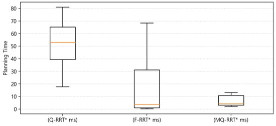
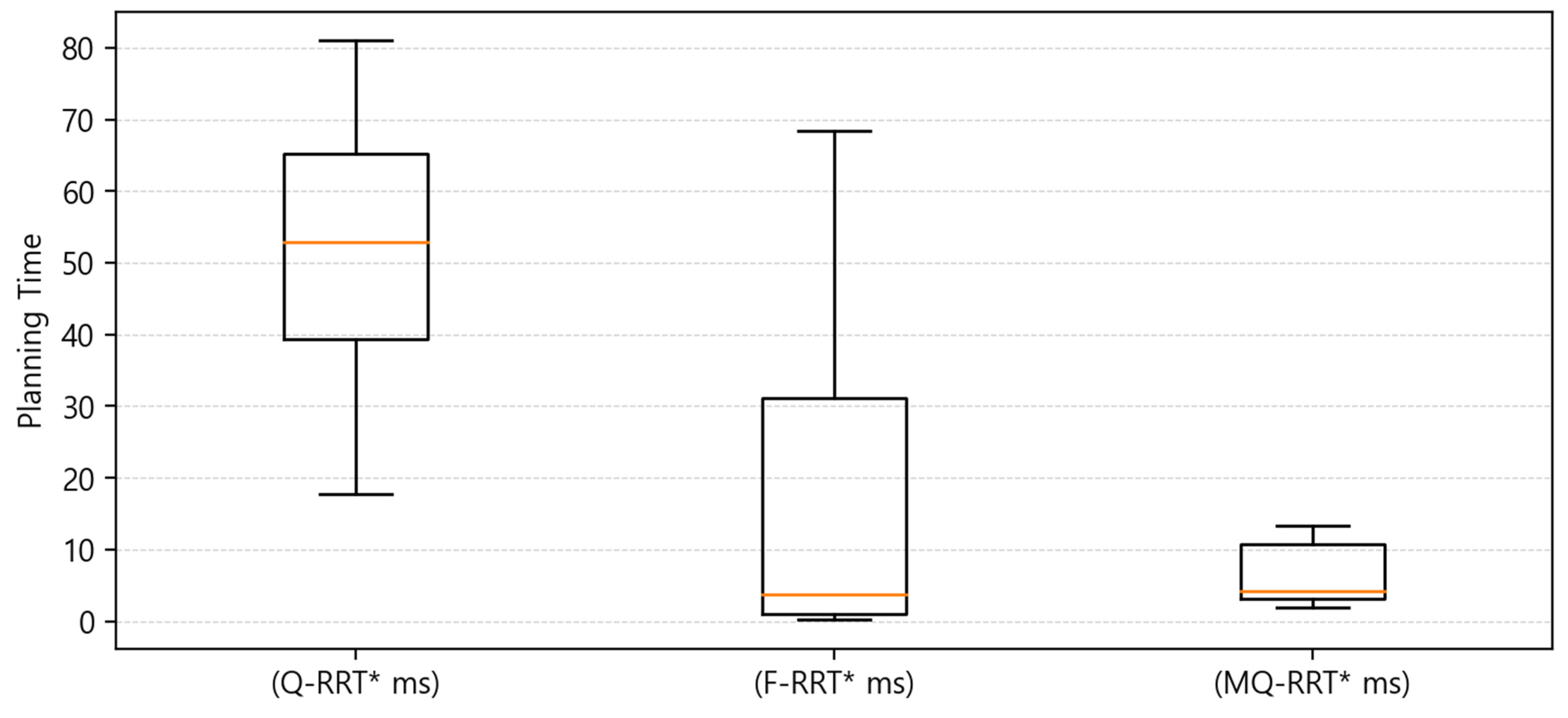
In Figure 11, for planning time, MQ-RRT* showed stable results as in Case $c_1$. In addition, the interquartile range (IQR) was narrow, indicating that the deviation between repeated experiments was the smallest. F-RRT* showed a low median. However, the upper whisker increased, indicating that the planning time was not consistent. In contrast, Q-RRT* showed a higher median than the other algorithms.

Figure 11. Box plot of the planning time results for Case $c_2$.

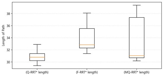
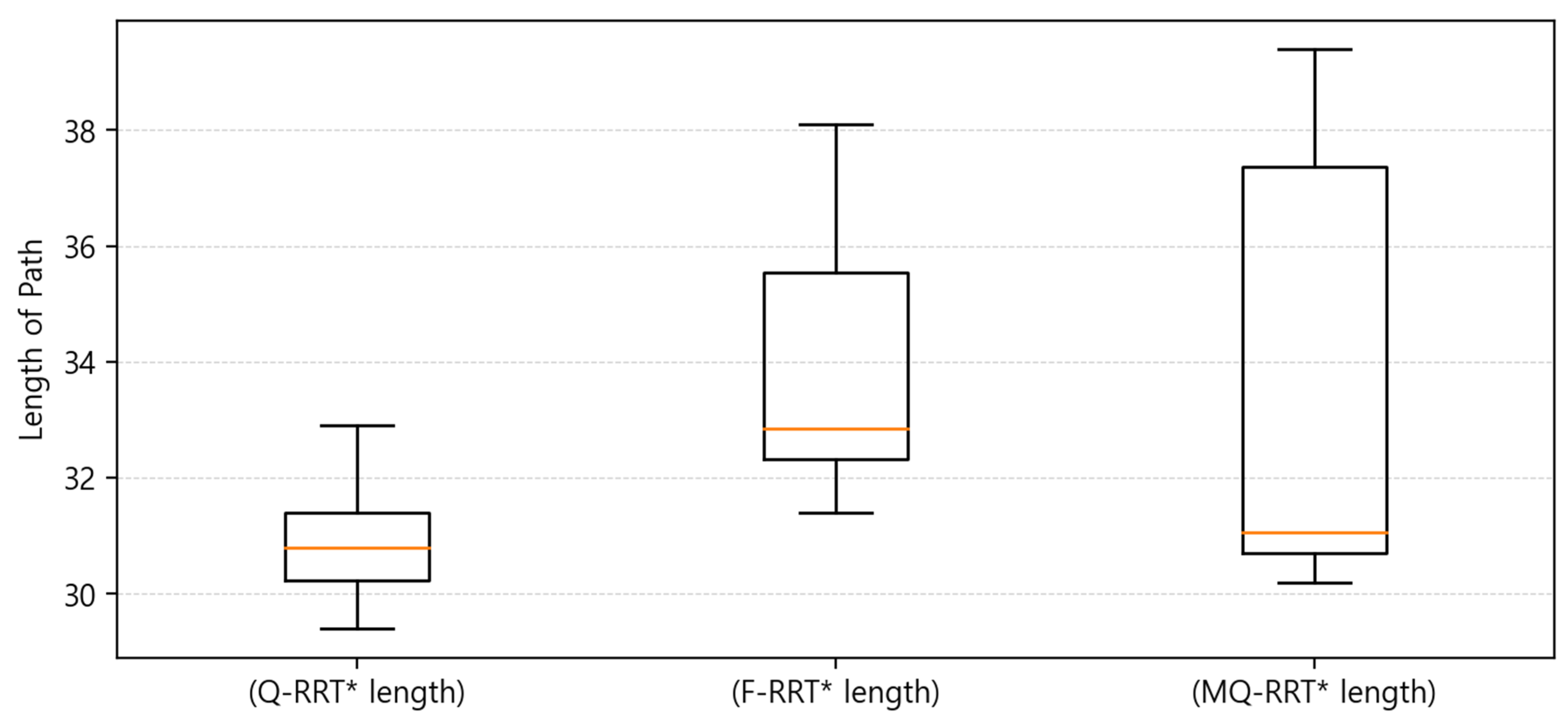
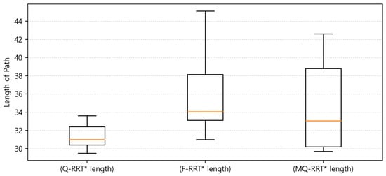
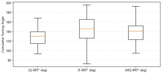
In Figure 12, for path length, Q-RRT* generated the shortest path. In Table 14, the median of Q-RRT* was the lowest at 30.80, and its IQR was also the narrowest at 1.18, indicating that the consistency of path length was the highest. MQ-RRT* had a median of 31.05, which was similar to that of Q-RRT*, but its IQR was 6.68, showing greater variation than Q-RRT*. In contrast, F-RRT* had the longest median value at 32.85 m, showing a disadvantageous result compared to the other algorithms in terms of path efficiency. In Figure 13, for cumulative turning angle, F-RRT* showed the lowest median. However, the width of its interquartile range box was the largest. In contrast, the box width of Q-RRT* was much smaller.

Figure 12. Box plot of the length of path results for Case $c_2$.

Table 14. Summary of the experimental results for Case $c_2$ (quartiles and standard deviation).

		Q1	Q2	Q3	IQR	Std.
Planning time (ms)	Q-RRT*	39.43	52.91	65.17	25.74	1176.55
	F-RRT*	0.97	3.80	31.14	30.17	70.43
	MQ-RRT*	3.18	4.15	10.67	7.49	61.55
Length of Path (m)	Q-RRT*	30.23	30.80	31.40	1.18	1.71
	F-RRT*	32.33	32.85	35.55	3.23	4.21
	MQ-RRT*	30.70	31.05	37.38	6.68	3.41
Cumulative turning angle (deg)	Q-RRT*	109.45	118.05	130.60	21.15	25.46
	F-RRT*	66.50	88.00	130.90	64.40	44.39
	MQ-RRT*	112.65	123.85	154.83	42.18	32.46

Figure 13. Box plot of the cumulative turning angle results for Case $c_2$.

Overall, MQ-RRT* showed the most stable performance in terms of planning time in Case $c_2$, but it was difficult to conclude that it was better than Q-RRT* in terms of path length and cumulative turning angle. Q-RRT* was somewhat disadvantageous in planning time, but it showed the best performance in length of path and the most stable results in cumulative turning angle. Meanwhile, F-RRT* had the lowest median planning time and the lowest median cumulative turning angle, but its large variability in both planning time and cumulative turning angle indicates limitations in terms of overall stability and consistency. In an environment such as Case $c_2$, F-RRT* and MQ-RRT* are heuristically recommended when fast path planning is desired. However, both algorithms show lower reliability in terms of path quality. Therefore, if one is willing to sacrifice some speed to ensure better path quality and safety, Q-RRT* is heuristically recommended.

In Case $c_3$, the performance of Q-RRT*, F-RRT*, and MQ-RRT* was compared in terms of planning time, length of path, and cumulative turning angle.

In Figure 14, Q-RRT* showed the slowest planning time compared to the other algorithms. It also showed that its consistency was not good. For F-RRT*, unlike Case $c_1$ and Case $c_2$, it was confirmed that it showed consistent results in Case $c_3$. The planning time performance of F-RRT* was measured to be the best. Figure 15 shows the results for length of path. Length of path showed the opposite tendency to planning time. Q-RRT* calculated the shortest path. Its stability and consistency were also better. The medians of MQ-RRT* and F-RRT* were similar. However, when looking at Figure 15 and the IQR values for length of path in Table 15, it can be seen that the interquartile box range of MQ-RRT* was large. For cumulative turning angle, Q-RRT* showed the lowest value. In Figure 16, F-RRT* showed a higher median than MQ-RRT*, and its interquartile range was also larger. This indicates that F-RRT* was less consistent than MQ-RRT*.

Figure 14. Box plot of the planning time results for Case $c_3$.

Figure 15. Box plot of the length of path results for Case $c_3$.

Table 15. Summary of the experimental results for Case $c_3$ (quartiles and standard deviation).

		Q1	Q2	Q3	IQR	Std.
Planning time (ms)	Q-RRT*	50.19	77.65	123.05	72.86	1137.20
	F-RRT*	0.80	2.23	6.64	5.84	125.97
	MQ-RRT*	8.58	14.23	38.76	30.18	150.59
Length of Path (m)	Q-RRT*	30.43	31.00	32.40	1.98	2.46
	F-RRT*	33.13	34.05	38.13	5.00	7.24
	MQ-RRT*	30.20	33.05	38.78	8.58	4.58
Cumulative turning angle (deg)	Q-RRT*	115.20	130.05	139.55	24.35	21.30
	F-RRT*	126.20	145.70	165.28	39.08	50.36
	MQ-RRT*	123.20	141.15	152.03	28.83	24.60

Figure 16. Box plot of the cumulative turning angle results for Case $c_3$.

Overall, Q-RRT* showed a slow planning time. However, the quality and consistency of the path were better than the other algorithms. But it showed that the performance and consistency in planning time were low. Case $c_3$ is similar to Case $c_2$. However, in Case $c_3$, a short shelf is present along the path to the goal point. In an environment such as Case $c_3$, F-RRT* is heuristically recommended when fast path planning is desired. However, as in the other cases, F-RRT* shows lower reliability in terms of path quality. Therefore, if one is willing to sacrifice speed to ensure better path quality and consistency, Q-RRT* is heuristically recommended. Overall, Q-RRT* showed a slow planning time. However, the quality and consistency of the path were better than the other algorithms. But it showed that the performance and consistency in planning time were low. Case $c_3$ is similar to Case $c_2$. However, in Case $c_3$, a short shelf is present along the path to the goal point. In an environment such as Case $c_3$, F-RRT* is heuristically recommended when fast path planning is desired. However, as in the other cases, F-RRT* shows lower reliability in terms of path quality. Therefore, if one is willing to sacrifice speed to ensure better path quality and consistency, Q-RRT* is heuristically recommended.

In Case $c_4$, the performance of Q-RRT*, F-RRT*, and MQ-RRT* was compared in terms of planning time, length of path, and cumulative turning angle.

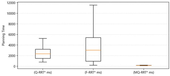
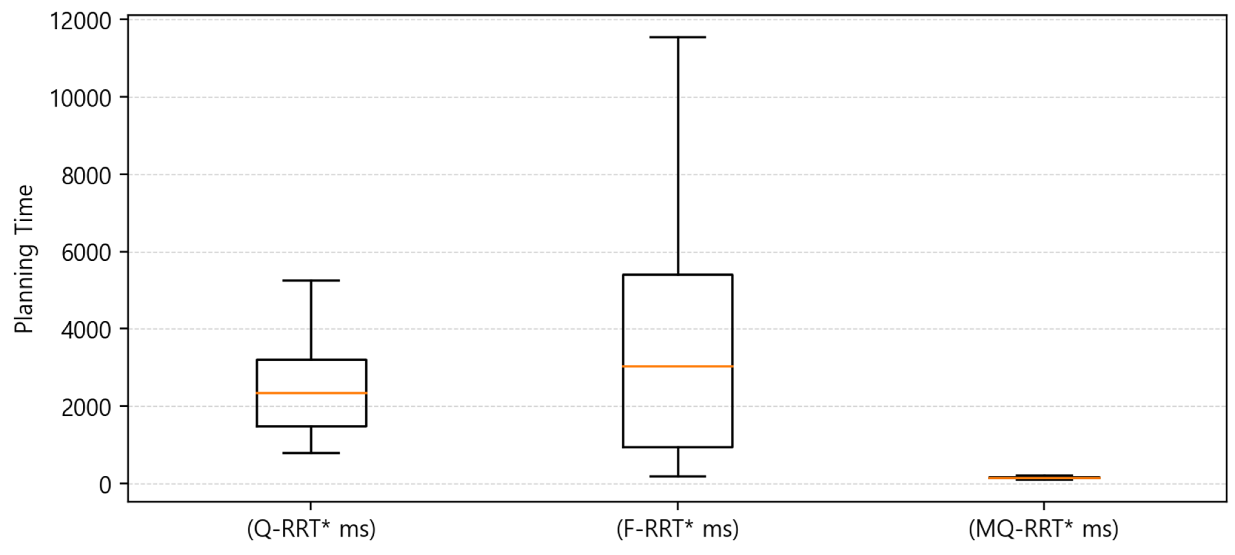
As shown in Figure 17, MQ-RRT* exhibited the best performance in terms of planning time. In Table 16, MQ-RRT* had the lowest median value of 160.42, and its IQR was also the narrowest at 32.20, indicating the smallest deviation among repeated experiments. In contrast, Q-RRT* showed a median value of 2348.60, which was higher than that of MQ-RRT*, while F-RRT* had the highest median value of 3032.45. In addition, F-RRT* showed the largest IQR of 4453.12, indicating the poorest consistency in planning time.

Figure 17. Box plot of the planning time results for Case $c_4$.

Table 16. Summary of the experimental results for Case $c_4$ (quartiles and standard deviation).

		Q1	Q2	Q3	IQR	Std.
Planning time (ms)	Q-RRT*	1486.10	2348.60	3212.12	1726.02	1153.83
	F-RRT*	953.49	3032.45	5406.60	4453.12	4728.21
	MQ-RRT*	143.01	160.42	175.21	32.20	22.62
Length of Path (m)	Q-RRT*	51.83	52.20	52.48	0.65	0.57
	F-RRT*	53.40	54.10	55.10	1.70	1.67
	MQ-RRT*	52.60	53.00	53.40	0.80	0.86
Cumulative turning angle (deg)	Q-RRT*	367.30	382.20	402.83	35.53	32.24
	F-RRT*	386.33	419.50	450.95	64.63	51.34
	MQ-RRT*	374.88	396.85	429.15	54.28	45.31

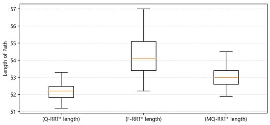
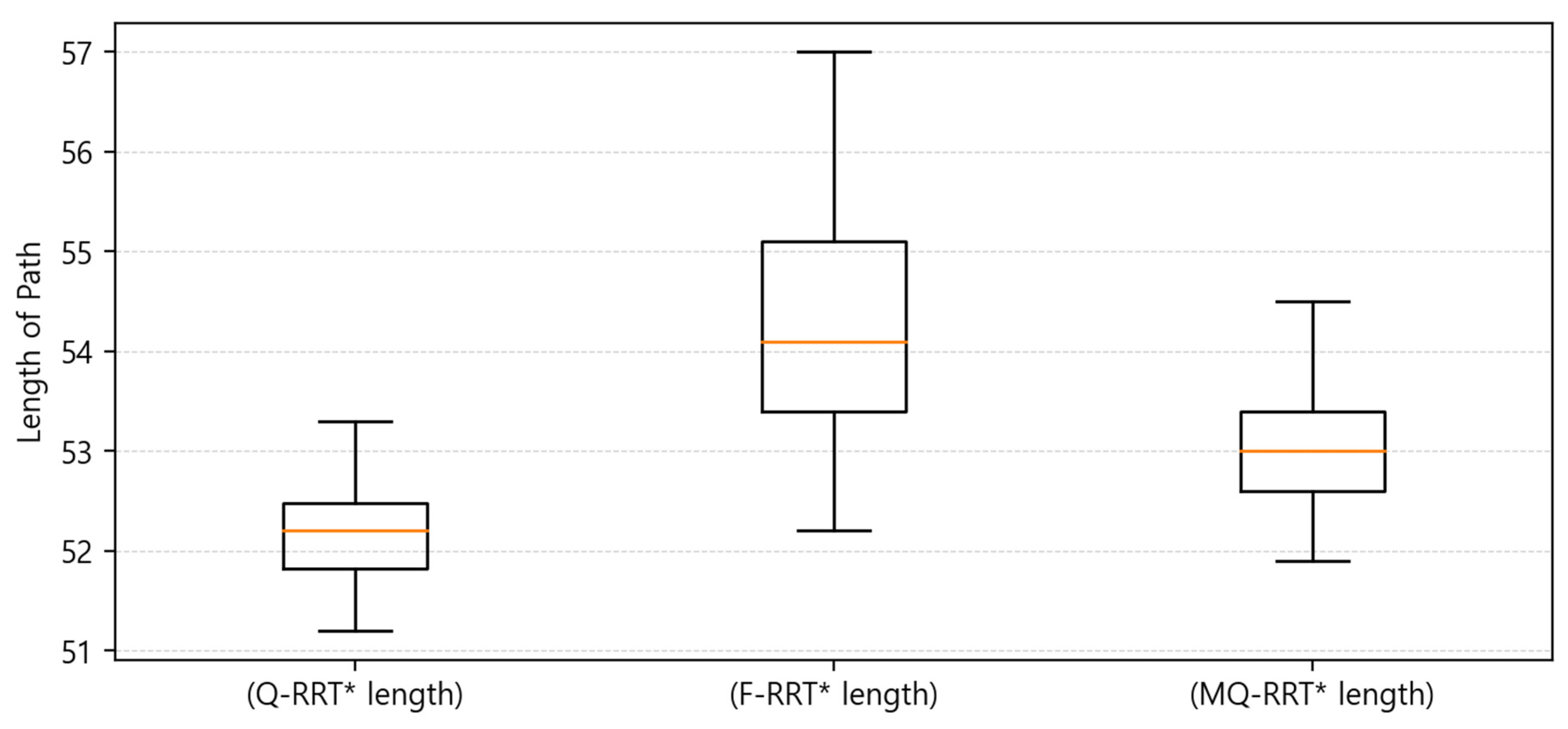
As shown in Figure 18, Q-RRT* generated the shortest path in terms of length of path. In Table 16, Q-RRT* had the lowest median value of 52.20, and its IQR was also the narrowest at 0.65, indicating the highest consistency in path length. MQ-RRT* had a median value of 53.00, indicating that it generated a slightly longer path than Q-RRT*. However, its IQR was 0.80, showing stable results. In contrast, F-RRT* had the highest median value of 54.10 m, and its IQR was also the largest at 1.70, indicating that it was inferior to the other algorithms in terms of path efficiency and consistency.

Figure 18. Box plot of the length of path results for Case $c_4$.

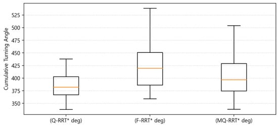
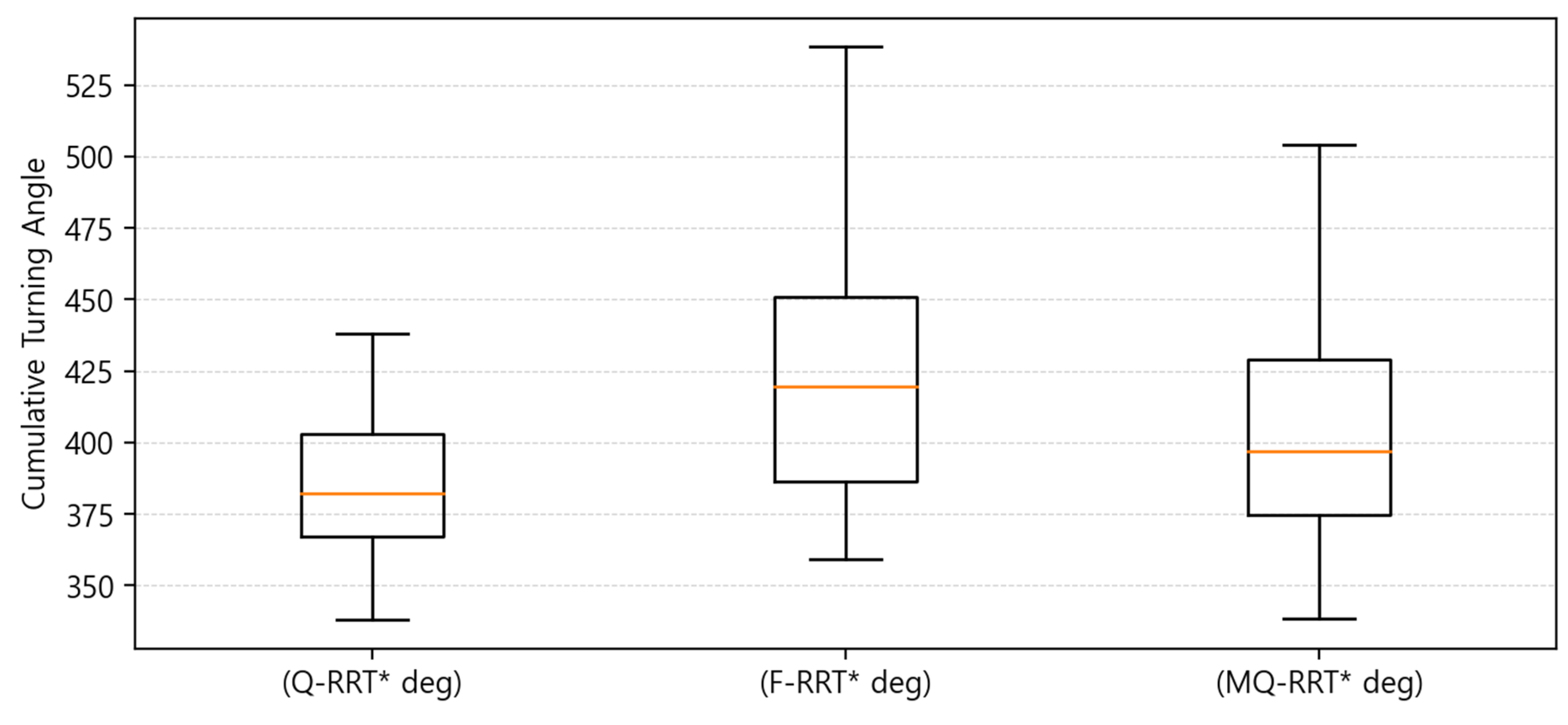
As shown in Figure 19, Q-RRT* showed the lowest median value in terms of cumulative turning angle. In Table 16, Q-RRT* had the lowest median value of 382.20, and its IQR was also the smallest at 35.53, indicating the most stable results. MQ-RRT* had a median value of 396.85, which was slightly higher than that of Q-RRT*, but lower than that of F-RRT*. In contrast, F-RRT* had the highest median value of 419.50, and its IQR was also the largest at 64.63, showing the poorest result in terms of cumulative turning angle.

Figure 19. Box plot of the cumulative turning angle results for Case $c_4$.

Overall, MQ-RRT* showed that it could compute paths both quickly and consistently in terms of planning time in Case $c_4$. However, Q-RRT* showed better results in terms of path length and cumulative turning angle. Although Q-RRT* was less favorable than MQ-RRT* in planning time, it generated the shortest path and also showed the most stable and best performance in cumulative turning angle. Meanwhile, F-RRT* was inferior to the other algorithms in the overall aspects of planning time, path length, and cumulative turning angle. In particular, it showed large variability in planning time and cumulative turning angle, indicating limitations in overall stability and consistency. Unlike the other cases, Case $c_4$ contains many turning sections along the path. In such an environment, MQ-RRT* is heuristically recommended when the path must be computed quickly. However, if path quality is prioritized and consistent results are desired even at the cost of longer planning time, Q-RRT* is heuristically recommended.

In Case $c_5$, the performance of Q-RRT*, F-RRT*, and MQ-RRT was compared in terms of planning time, path length, and cumulative turning angle.

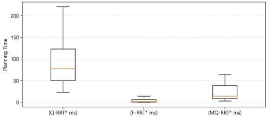
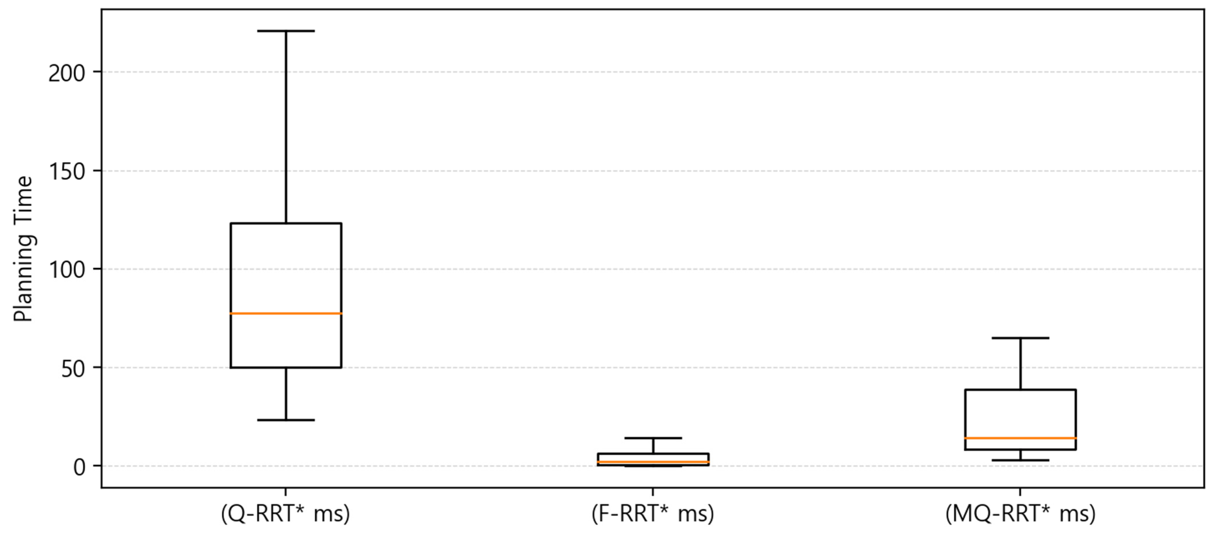
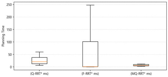
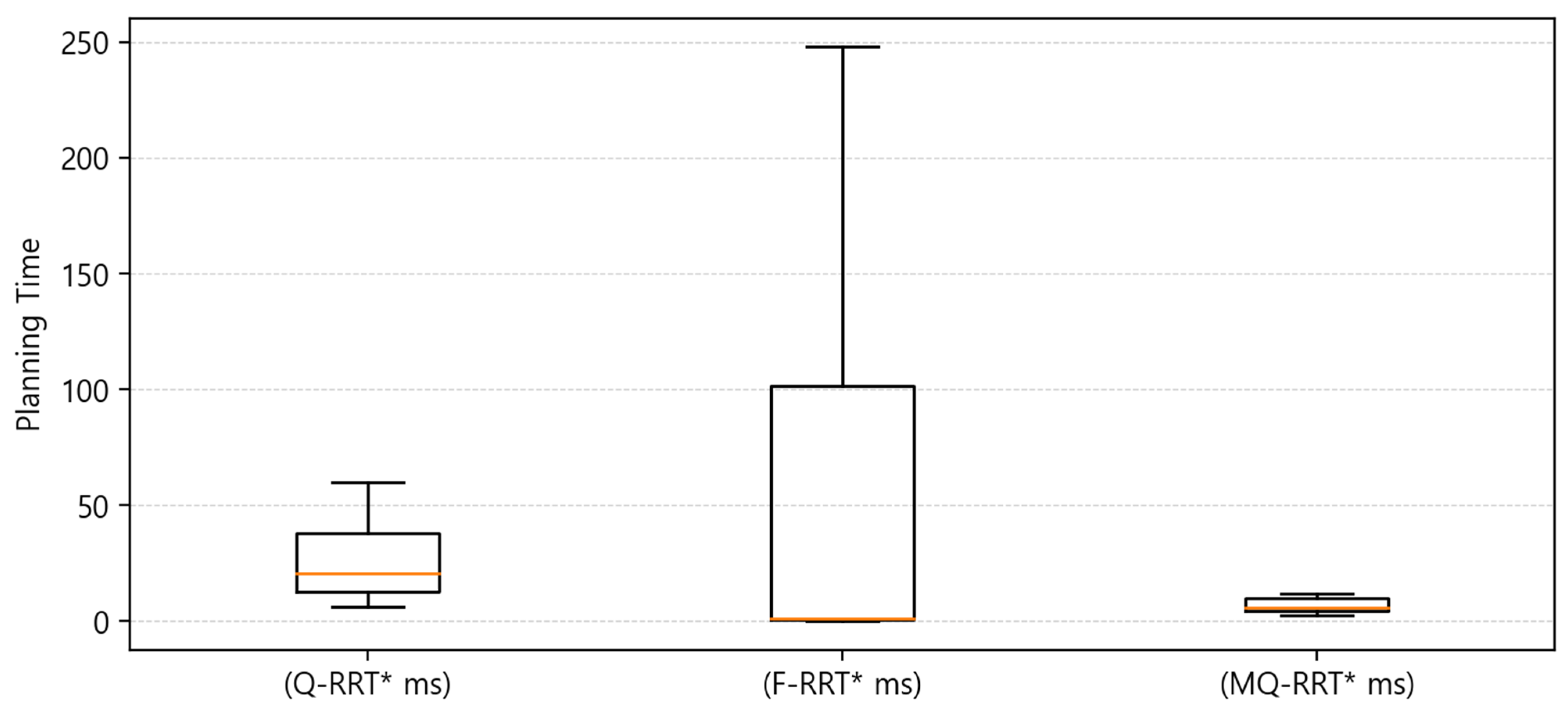
As shown in Figure 20 and Table 17, F-RRT exhibited the fastest performance in terms of planning time. F-RRT had the lowest median value, at 1.16 ms. However, its IQR was the largest at 100.91, indicating that the variation in planning time was large. In contrast, MQ-RRT had a median value of 5.58 ms, which was somewhat slower than that of F-RRT, but it showed the highest consistency, with the smallest IQR of 5.67 and the lowest standard deviation of 47.74. Q-RRT had the slowest performance among the three algorithms, with a median value of 20.55 ms, and its IQR was also larger than that of MQ-RRT*, at 25.36.

Figure 20. Box plot of the planning time results for Case $c_5$.

Table 17. Summary of the experimental results for Case $c_5$ (quartiles and standard deviation).

		Q1	Q2	Q3	IQR	Std.
Planning time (ms)	Q-RRT*	12.74	20.55	38.10	25.36	1044.63
	F-RRT*	0.59	1.16	101.50	100.91	292.04
	MQ-RRT*	4.40	5.58	10.07	5.67	47.74
Length of Path (m)	Q-RRT*	31.03	35.70	36.70	5.68	3.27
	F-RRT*	32.30	35.25	38.10	5.80	5.23
	MQ-RRT*	31.03	35.35	35.80	4.78	2.70
Cumulative turning angle (deg)	Q-RRT*	84.00	90.10	99.55	15.55	12.78
	F-RRT*	67.35	86.90	96.48	29.13	31.35
	MQ-RRT*	84.65	88.60	97.80	13.15	12.20

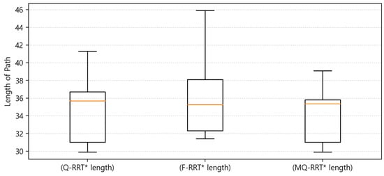
The path length results shown in Figure 21 indicate that, based on the median values, F-RRT generated the shortest path, at 35.25 m. The median path length of MQ-RRT was 35.35 m, which was similar to that of F-RRT, whereas Q-RRT had the largest value among the three algorithms, at 35.70 m, although the difference was not substantial. However, in terms of consistency, MQ-RRT was the most stable. MQ-RRT had the smallest IQR, at 4.78, and the lowest standard deviation, at 2.70, indicating the most stable performance in terms of path length. In contrast, although F-RRT had the lowest median value, it also had the largest IQR, at 5.80, and the highest standard deviation, at 5.23, indicating that the variation in path length was the largest. In other words, in the Case $c_5$ environment, F-RRT has the potential to produce superior results in terms of path length, but the stability of its results can be interpreted as relatively low.

Figure 21. Box plot of the cumulative turning angle results for Case $c_5$.

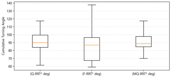
For the cumulative turning angle results shown in Figure 22, F-RRT had the lowest median value, at 86.90 deg. MQ-RRT followed with 88.60 deg, while Q-RRT had the highest median value, at 90.10 deg. However, in this metric as well, MQ-RRT showed the best consistency. In contrast, although F-RRT had the lowest median value, it also had the largest IQR, at 29.13, and the highest standard deviation, at 31.35. Q-RRT was the least favorable in terms of the median value, but its variation was smaller than that of F-RRT.

Figure 22. Box plot of the cumulative turning angle results for Case $c_5$.

Overall, in Case $c_5$, F-RRT showed the best performance in terms of the median values of planning time, path length, and cumulative turning angle. However, the variation was large across all three metrics, indicating that the consistency of the results was relatively low. In contrast, the median values of MQ-RRT were slightly less favorable than those of F-RRT for each metric. Nevertheless, MQ-RRT showed the most stable and consistent performance overall. Q-RRT imposed the greatest computational burden in terms of planning time and did not show any clear advantage in either path length or cumulative turning angle. Therefore, in an environment such as Case $c_5$, F-RRT may be considered when fast computation time and superior median performance are important. However, when the stability of the results and the overall balance are also taken into account, MQ-RRT can be regarded as being heuristically recommended.

4.8. Discussion

Experiments were conducted for each algorithm in a warehouse environment. The results show that even under the same environment and the same goal position, performance differences existed depending on the value of $r_{\mathrm{near}}$. Overall, as $r_{\mathrm{near}}$ increased, the number of candidate neighboring nodes considered increased, and planning time increased.

In contrast, the path quality metrics, path length and cumulative turning angle, improved as $r_{\mathrm{near}}$ increased, but after a certain range, the amount of quality improvement was limited. That is, the improvement in path quality was not large compared to the increase in planning time. This means that when $r_{\mathrm{near}}$ is too small, only a small number of neighboring nodes are considered, and an inefficient path is generated because few nodes are considered. It also means that considering neighbors beyond a certain level involves considering unnecessary nodes, which results in increased computation.

When applying the heuristically chosen $r_{\mathrm{near}}$ for each algorithm, MQ-RRT* generally showed strengths in computation speed. In contrast, Q-RRT* showed relatively slow planning time and large variability, but it showed strengths in path length and cumulative turning angle. F-RRT* had limited stability because its variability was large.

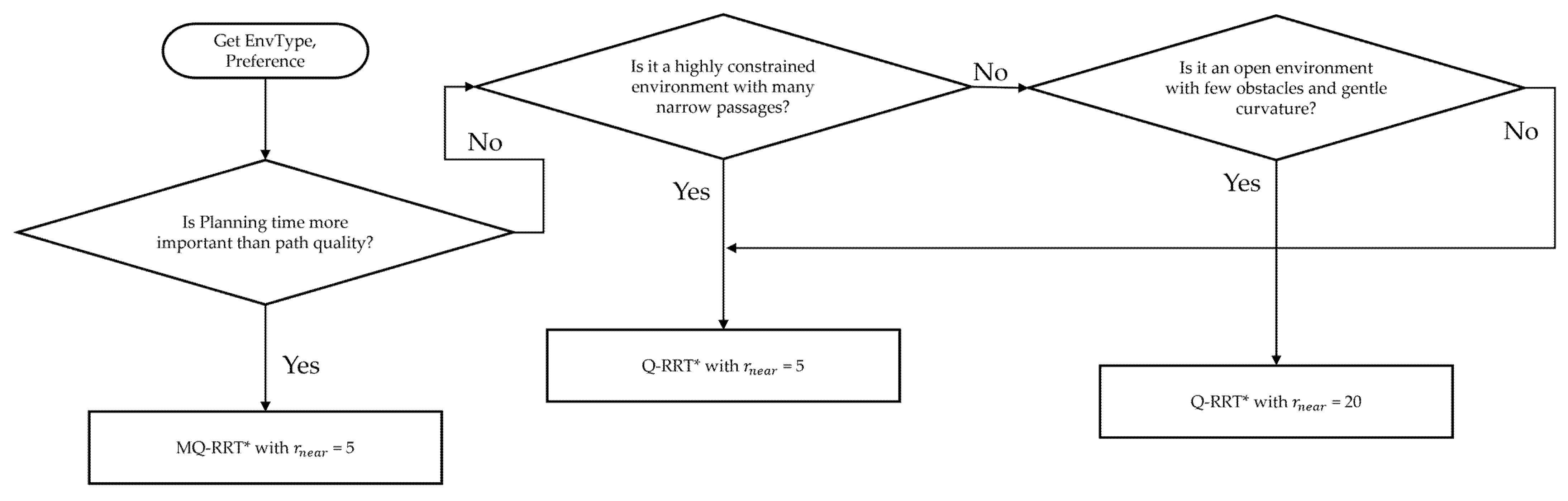
In summary, increasing $r_{\mathrm{near}}$ from a small value to a certain range improved path quality, while beyond a certain level, the benefit in path quality was limited compared to the increase in planning time. Also, the heuristically chosen $r_{\mathrm{near}}$ differed depending on the mechanisms of each algorithm. It was confirmed that the same increase in $r_{\mathrm{near}}$ can improve quality in some cases, but in other cases it can only increase time or even worsen quality. Therefore, if real-time performance is required, MQ-RRT* can be an option. If path length or cumulative turning angle is prioritized, Q-RRT* can be an option. Figure 23 is a flowchart that heuristically chosen an appropriate algorithm and parameter according to the environment and the user’s preference, based on the above results. The environment and the user’s preference are taken as inputs. If faster planning time is preferred over path quality, MQ-RRT* is heuristically chosen. If path quality is prioritized, the recommended algorithm and $r_{near}$ value are determined by dividing the situation into three major cases. In the case of F-RRT*, its large variability made it limited in terms of being heuristically chosen.

Figure 23. A flowchart for heuristically selecting an algorithm according to the user’s preference and the environment.

5. Conclusions

This paper analyzed the effect of the neighbor radius parameter $r_{\mathrm{near}}$ on the performance of RRT*-based algorithms used for sampling-based path planning of mobile robots in a warehouse environment. We selected Q-RRT*, F-RRT*, and MQ-RRT* for comparison. Experiments were conducted in a ROS2 Humble and Gazebo Harmonic simulation environment. The experiments were divided into four cases. Performance metrics were planning time, length of path, and cumulative change in turning angle. Lower values indicate better performance for all metrics.

The results show that as $r_{\mathrm{near}}$ increased, all three algorithms improved path length and cumulative turning angle up to a certain range. After that, the values remained within a limited range. This confirms that $r_{\mathrm{near}}$ is a parameter that determines path quality. However, planning time did not show the same behavior. For Q-RRT* and MQ-RRT*, planning time increased as $r_{\mathrm{near}}$ increased. F-RRT* showed a similar tendency in Case $c_1$. In other cases, planning time showed large fluctuations with increases and decreases across ranges. This indicates that an appropriate $r_{\mathrm{near}}$ should be selected depending on the environment. It also implies that generalization can be limited when a fixed parameter is applied.

Based on repeated experiments in each case, we selected the heuristically chosen $r_{\mathrm{near}}$ for each algorithm. In Case $c_1$, $r_{\mathrm{near}}=5$ was selected as the heuristically chosen value for Q-RRT*, F-RRT*, and MQ-RRT*. In Case $c_2$, the heuristically chosen values were 20 for Q-RRT*, 30 for F-RRT*, and 5 for MQ-RRT*. In Case $c_3$, the heuristically chosen values were 20 for Q-RRT*, 20 for F-RRT*, and 5 for MQ-RRT*. In Case $c_4$, the heuristically chosen values were 5 for Q-RRT*, 5 for F-RRT*, and 5 for MQ-RRT*. In Case $c_5$, the heuristically chosen values were 5 for Q-RRT*, 1 for F-RRT*, and 5 for MQ-RRT*.

The comparison results under the heuristically chosen parameter conditions showed that F-RRT* achieved fast planning time in most cases; however, its results were inconsistent. In terms of planning time, MQ-RRT* showed the next best performance after F-RRT*. In addition, it demonstrated more consistent results than the other algorithms in most cases. Q-RRT* showed relatively slow planning time. However, it tended to generate shorter paths with less turning than the other algorithms. Therefore, when applying RRT*-based algorithms in a warehouse environment, Q-RRT* can be an option if path quality is prioritized and an increase in planning time can be accepted. In contrast, MQ-RRT* can be suitable if fast path planning and relatively stable results are prioritized.

Overall, this study quantitatively presented how the setting of $r_{\mathrm{near}}$ affects the performance of RRT*-based sampling path planning algorithms in a warehouse environment. It also provided evidence and guidelines for selecting $r_{\mathrm{near}}$ for each algorithm by considering planning time and path quality metrics together.

Future work should extend the evaluation by adding more diverse warehouse environments. This study did not perform a quantitative classification of the terrain structure from the start position to the goal position. Therefore, additional analysis is needed to characterize terrain structure and to separate and compare results across segments with similar characteristics. Finally, since this study analyzed the effect of parameter changes on algorithm performance in a simulation environment only, all experiments were conducted on a desktop platform. As a result, performance on embedded hardware systems that may be used in actual mobile robots, such as Raspberry Pi or NVIDIA Jetson series devices, was not evaluated. Further validation on such hardware systems is needed.

References

- Gervasoni, J.; Pedrazzini, D.; Cicchinelli, M.; Persichilli, S.; Baroni, S.; Rocchetti, S.; Arcuri, G.; Urbani, A. Impact of an autonomous delivery robot on sample turnaround time in a clinical laboratory: An early evaluation of first implementation. Clin. Chem. Lab. Med. 2025, 64, 832–837. [Google Scholar] [CrossRef] [Scilit]
- Croghan, S.M.; Carroll, P.; Reade, S.; Gillis, A.E.; Ridgway, P.F. Robot Assisted Surgical Ward Rounds: Virtually Always There. J. Innov. Health Inform. 2018, 25, 41–56. [Google Scholar] [CrossRef] [Scilit] [PubMed]
- Roshanianfard, A.; Noguchi, N.; Ardabili, S.; Mako, C.; Mosavi, A. Autonomous Robotic System for Pumpkin Harvesting. Agronomy 2022, 12, 1594. [Google Scholar] [CrossRef] [Scilit]
- Imaoka, K.; Emaru, T. Pulling-Out Weeding Device for Intra-Row Weeding Robots. In Proceedings of the 2024 IEEE/SICE International Symposium on System Integration (SII), Ha Long, Vietnam, 8–11 January 2024; pp. 747–752. [Google Scholar]
- Auh, E.; Kim, J.; Joo, Y.; Park, J.; Lee, G.; Oh, I.; Pico, N.; Moon, H. Unloading sequence planning for autonomous robotic container-unloading system using A-star search algorithm. Eng. Sci. Technol. Int. J. 2024, 50, 101610. [Google Scholar] [CrossRef] [Scilit]
- Žulj, I.; Salewski, H.; Goeke, D.; Schneider, M. Order batching and batch sequencing in an AMR-assisted picker-to-parts system. Eur. J. Oper. Res. 2022, 298, 182–201. [Google Scholar] [CrossRef] [Scilit]
- Zhou, Y.; Yan, L.; Han, Y.; Xie, H.; Zhao, Y. A Survey on the Key Technologies of UAV Motion Planning. Drones 2025, 9, 194. [Google Scholar] [CrossRef] [Scilit]
- Xu, T. Recent advances in Rapidly-exploring random tree: A review. Heliyon 2024, 10, e32451. [Google Scholar] [CrossRef] [Scilit] [PubMed]
- Hu, M.; Huang, Q.; Cai, J.; Chen, Y.; Li, J.; Shi, L. HPS-RRT*: An Improved Path Planning Algorithm for a Nonholonomic Orchard Robot in Unstructured Environments. Agronomy 2025, 15, 712. [Google Scholar] [CrossRef] [Scilit]
- Faroni, M.; Pedrocchi, N.; Beschi, M. Adaptive hybrid local–global sampling for fast informed sampling-based optimal path planning. Auton. Robot. 2024, 48, 6. [Google Scholar] [CrossRef] [Scilit]
- Jeong, I.-B.; Lee, S.-J.; Kim, J.-H. Quick-RRT*: Triangular inequality based implementation of RRT* with improved initial solution and convergence rate. Expert Syst. Appl. 2019, 123, 82–90. [Google Scholar] [CrossRef] [Scilit]
- Liao, B.; Wan, F.; Hua, Y.; Ma, R.; Zhu, S.; Qing, X. F-RRT*: An improved path planning algorithm with improved initial solution and convergence rate. Expert Syst. Appl. 2021, 184, 115457. [Google Scholar] [CrossRef] [Scilit]
- Cui, X.; Wang, C.; Xiong, Y.; Mei, L.; Wu, S. More Quickly-RRT*: Improved Quick Rapidly-exploring Random Tree Star algorithm based on optimized sampling point with better initial solution and convergence rate. Eng. Appl. Artif. Intell. 2024, 133, 108246. [Google Scholar] [CrossRef] [Scilit]
- LaValle, S.M. Rapidly-Exploring Random Trees: A New Tool for Path Planning; Springer: London, UK, 1998. [Google Scholar]
- Gao, H.; Liu, D.; Hu, J. A Survey on Path Planning for Mobile Robot Systems. In Proceedings of the 2023 IEEE 12th Data Driven Control and Learning Systems Conference (DDCLS), Xiangtan, China, 12–14 May 2023; pp. 1176–1181. [Google Scholar]
- Jung, J.-W.; So, B.-C.; Kang, J.-G.; Lim, D.-W.; Son, Y. Expanded Douglas–Peucker Polygonal Approximation and Opposite Angle-Based Exact Cell Decomposition for Path Planning with Curvilinear Obstacles. Appl. Sci. 2019, 9, 638. [Google Scholar] [CrossRef] [Scilit]
- Zuo, S.; Mao, Z.; Fan, C.; Chen, X.; Gong, M.; Ren, J.; Fan, X.; Guo, Y. Dynamic planning of crowd evacuation path for metro station based on Dynamic Avoid Smoke A-Star algorithm. Tunn. Undergr. Space Technol. 2024, 154, 106145. [Google Scholar] [CrossRef] [Scilit]
- Jeon, G.-Y.; Jung, J.-W. Water Sink Model for Robot Motion Planning. Sensors 2019, 19, 1269. [Google Scholar] [CrossRef] [Scilit] [PubMed]
- Gammell, J.D.; Srinivasa, S.S.; Barfoot, T.D. Informed RRT*: Optimal Sampling based Path Planning Focused via Direct Sampling of an Admissible Ellipsoidal Heuristic. In Proceedings of the IEEE/RSJ International Conference on Intelligent Robots and Systems, Chicago, IL, USA, 14–18 September 2014; pp. 2997–3004. [Google Scholar]
- Naderi, K.; Rajamäki, J.; Hämäläinen, P. RT-RRT*: A Real-Time Path Planning Algorithm Based on RRT*. In Proceedings of the 8th ACM SIGGRAPH Conference on Motion in Games (MIG ′15), Paris, France, 16–18 November 2015; pp. 113–118. [Google Scholar]
- Armstrong, D.; Jonasson, A. AM-RRT*: Informed Sampling-Based Planning with Assisting Metric. In Proceedings of the 2021 IEEE International Conference on Robotics and Automation (ICRA), Xi’an, China, 30 May–5 June 2021; pp. 10093–10099. [Google Scholar]
- Nasir, J.; Islam, F.; Malik, U.; Ayaz, Y.; Hasan, O. RRT*-Smart: Rapid Convergence Implementation of RRT* towards Optimal Solution. Int. J. Adv. Robot. Syst. 2013, 10, 299. [Google Scholar] [CrossRef] [Scilit] [PubMed]
- Jeong, J.; Jung, J.-W. Fast Path-Planning Algorithm for Mobile Robots via Straight Strategy. Appl. Sci. 2026, 16, 1952. [Google Scholar] [CrossRef] [Scilit]
- Villagra, J.; Milanés, V.; Pérez, J.; Godoy, J. Smooth path and speed planning for an automated public transport vehicle. Robot. Auton. Syst. 2012, 60, 252–265. [Google Scholar] [CrossRef] [Scilit]
Disclaimer/Publisher’s Note: The statements, opinions and data contained in all publications are solely those of the individual author(s) and contributor(s) and not of MDPI and/or the editor(s). MDPI and/or the editor(s) disclaim responsibility for any injury to people or property resulting from any ideas, methods, instructions or products referred to in the content. |
© 2026 by the authors. Licensee MDPI, Basel, Switzerland. This article is an open access article distributed under the terms and conditions of the Creative Commons Attribution (CC BY) license.