


Featured Application
Adaptive systems are essential for controlling, for example, vehicles whose mass changes with fuel consumption, such as small unmanned aerial vehicles, rockets, and so on. Adaptive systems also solve problems of controlling chemical reactions, where the state of the mathematical model of the controlled process changes over time as the reaction proceeds. Adaptive systems are also important for controlling robots and manipulators that operate with variable drives or carry objects with variable masses. The scope of application of adaptive systems is as broad as the area requiring control of non-stationary objects.
Abstract
Control of dynamic technical objects in locked-loop systems with negative feedback is widely used in robotics and all complex technical devices. The theory of ensuring accuracy, speed, and control quality is well developed for the case of stationary objects. If the parameters of the controlled object change over time, the development of adaptive systems is recommended. Many articles and monographs have been written on the topic of adaptive control, but most often they provide only general indications that an additional external loop is necessary to change the controller parameters so that the modified controller more successfully ensures control accuracy and quality than its previous version. At the same time, methods for solving the two most complex sub-problems almost never were disclosed: determining how exactly the mathematical model of the object has changed and deciding how exactly the controller parameters should be changed to provide the required properties of the system as a whole. This paper proposes some general principles for designing adaptive systems and demonstrates their effectiveness using several examples.
1. Introduction
The principle of high-gain negative feedback in control loop has been successfully used for long time. It allows for the significant suppression of control errors, including those arising from disturbance that cannot be predicted or measured.
The properties of a system depend significantly on the properties of the complex transfer function of its open loop . Here , is the phase-frequency characteristic of the open loop, and is the amplitude-frequency characteristic of the open loop. Depending on the response speed of an object, automatic control theory distinguishes three frequency ranges: low frequencies, mid frequencies, and high frequencies. The criterion for this division is the absolute value of the transfer function of the entire system circuit .
At low frequencies, where , the error suppression is achieved very large: in times. In this frequency range, the controlled state of the object, called the “output signal,” follows the command rather precisely. The system has zero static error if , which is the case for a system with an integrator in the object model or in the controller model. In the high frequency region, where , feedback ceases to influence the operation of the object, because at these frequencies the gain of the circuit is much less than the unity gain. The mid-frequency range lies between the low and high frequencies. In this range . The type of frequency response of the loop in this frequency range determines the stability of the system and its quality in terms of the dynamic properties of the transient process. These quality indicators include stability margin, overshoot, and the amount of oscillation, if any.
The low-frequency part of the loop must have a simple property: the absolute value of the transfer function must be as large as possible. Changes in this transfer function by even a factor of 1.5 or more are not critical, as it typically developers provide a sufficiently large value of with a large margin. The high-frequency part of the loop must also have a very simple property: the absolute value of the transfer function in this range must be sufficiently small, and small changes in this transfer function, even by 1.5–2 times, are also not critical. The mid-frequency range of the loop is the most important and most vulnerable property of a locked-loop system. In some cases, changes to this function can significantly affect the properties of the entire system. A previously stable system may become unstable.
The open-loop transfer function is equal to the product of the controller’s transfer function and the object’s transfer function. If the object’s transfer function is not stationary and changes uncontrollably, then the entire open-loop transfer function also changes uncontrollably, which can lead to a loss of stability. In this case, the system will be unable to perform its intended function. To provide the required properties of the system as a whole, whenever the object’s transfer function changes, it is necessary to make corresponding changes to the controller’s transfer function so that the product of these two transfer functions always meets the required properties.
These problems are solved by systems that are called adaptive, because the mathematical model of the regulator adapts to the properties of the object [1,2].
When changes in the object’s transfer function are known, adjusting the controller is straightforward. For example, if we know that the object’s transfer coefficient has increased by the factor , then it is sufficient to reduce the controller’s overall gain by the same factor . This case presents no scientific challenge and is not considered further.
Another class of adaptive systems are those where the precise time evolution of the object’s transfer function is unknown. The problem would be extremely complex if the object’s mathematical model were to change dramatically. For example, if not only the values of the object’s model coefficients but also the overall appearance of the model—that is, the model’s structure—change, then even general recommendations for creating an adaptive system are very difficult to provide. In simpler situations, only a few coefficients of the object’s mathematical model change.
One example is changing only the gain of an object. However, even in this case, without the ability to measure and track these changes, technical solutions are required to resolve this problem effectively. Such systems must adjust the controller’s gain so that the system as a whole remains stable, with the absence of information about changes in the object’s gain
One way to solve this problem is to identify precursors to instability and make preventive changes to the gain. However, the literature contains general adaptive system structures that, according to the authors, effectively maintain system stability when the mathematical model of the object changes in an uncontrolled manner. The problem is that such structures contain at least one element whose operating principle is only stated in general terms but is not disclosed in such detail that other users based on the literature describing of such structures could apply these ideas.
Publications describing such systems often claim that these structures are effective regardless of how the object’s transfer functions change. This is a clear exaggeration.
The changes in the object model must be such that in the mid-frequency region, where , it would remain possible to ensure the desired type of function due to the corresponding changes in the transfer function of the controller.
There are the properties of the resulting system in this range that influence the behavior of the system as a whole. It is required that in the region where , the requirement be satisfied . For minimum-phase systems (that is, for systems without pure delay elements), the phase characteristic is uniquely related to the slope of the amplitude characteristic .
The slope is a boundary value. With a sharper slope, the system is unstable; with a smoother slope, the system is stable. For example, with a slope, there is no overshoot in the system. With the intermediate slope value in this area the system is formally stable but may be prone to oscillations and overshoot.
When the gain in the object’s transfer function changes, the slope of the characteristic does not change, but the entire characteristic changes in magnitude. Therefore, the point where the transfer function passes near unity shifts up or down in frequency, which can violate the stability requirement. In this case, the system becomes unstable.
As a rule, the essence of an adaptive system is that the main control loop is considered as a new composite object, and around the new object an external system is created, for which the control object is the parameters of the main loop controller, and the input signals are the properties of this main system [1,2].
The literature presents a rich set of very schematic structures of adaptive systems, a brief overview of which is given in Appendix A. Among these structures, many technical solutions that are presented so laconically that only in general terms is it clear by what principle such a system should function, but the operating algorithms of the most essential elements of such systems are completely unclear. In the review books (see Appendix A) the mathematical models of objects and links for adaptation are not specified, and a clear description of the main adaptation algorithm is not given. Readers can only guess what the initial signals in such a system are and how these initial signals are transformed into the required changes or new values of the main loop controller. In addition, almost all such adaptive systems described in this literature use the features of the system’s response to a changing of the task signal V(t) to impart adaptive properties to the system. Therefore, such structures are unacceptable for the creation of adaptive stabilization systems, since in stabilization systems the task is constant, its change is zero, and, consequently, the changing of output signals of all links of the structural diagram fed by this task are also zero, and the existence of such connections does not affect the properties of the locked-loop system. Therefore, such systems do not impart adaptive properties to such system. This fact forces us to critically rethink similar structures, an example of which is given in Appendix A. Only those structural schemes should be considered or proposed whose functionality is preserved even when the system’s task signal is zero.
The most recent publications in this area also have similar shortcomings, and they are very specific. In article [1], the self-tuning unit is fed by an error signal and a signal from the controller output and also receives the “Initial Tuning” and “Parameters” signals. The object model lacks a delay element, the algorithm for calculating the new PID controller coefficients based on these signals is not entirely clear, and the origin of the “Initial Tuning” and “Parameters” signals is also unclear. The article [2] proposes a variable forgetting factor for the PID controller signal, which is related to the integral component. Adaptation has a narrow application; it is intended to adjust the forgetting factor. The article [3] proposes an adaptive controller for quadcopter UAVs. Stability analysis is performed using the Lyapunov method; no delay element is found in the object model; the results are obtained through simulation in MATLAB (version 7.11). The article [4] proposes an adaptive system for an inverted pendulum, in which the adaptation algorithm is based on the analysis of oscillations during a transient process initiated by stepwise jumps in the task. This method is difficult to apply to obtaining the adaptive properties of a stabilization system, since such jumps are undesirable during the operation of such a system. The model also does not include delays; the results are obtained by simulation. The article [5] proposes an adaptive PID control based on the Laplace distribution for temperature control under various environmental conditions in intelligent refrigeration systems. The object’s model is delay-free, and the concept is validated using simulations. In the article [6], an adaptive PID controller for active vehicle suspension based on neural networks is proposed. The object model is delay-free, and the algorithm is validated using simulation. The article [7] describes the application of an agent-based algorithm using artificial intelligence for adaptive PID control of a servomotor in real time. The motor model is delay-free, and the concept was validated using simulation. In the article [8], a fuzzy adaptive PID control strategy based on particle swarm optimization is proposed to ensure fast and stable control of a vehicle’s auxiliary power unit. The object model is given in difference equations, delay is ignored, and the results are verified using numerical simulation. The article [9] also proposes a neural network for adaptive tuning of a PID controller in a high-temperature heating system. The plant model does not take into account the delay, and the results are verified by simulation. The article [10] addresses the problem of self-consistent PID control with an adaptive transition function to improve position tracking of an electronic throttle valve. A derivative link from the setpoint signal to the controller is used, the model is delay-free, verification is performed by simulation, and experiments with a prototype are conducted. In the article [11], an adaptive fractional-order PID controller design is proposed for a high-power dual-channel active bridge DC-DC converter. This system is enhanced using a multi-agent deep deterministic gradient behavior algorithm for electric vehicles. The object model is represented as an electrical RLC four-terminal, and the results are verified by simulation. In the article [12], an adaptive PID control using a sliding mode is proposed for tracking the position of a quadcopter. The model does not take into account delay, and simulations and evaluations are performed under real conditions. The article [13] presents the results of a study of an adaptive PID control system with fuzzy logic for tracking the sun on solar panels with a variable parameter range. The mathematical model of the object does not contain any delay. The article [14] proposes adaptive PID control for hydroelectric power plants based on particle swarm optimization and fuzzy inference. The adaptation device interacts only with the hydrodynamic turbine, from which it reads signals and to which it receives control signals. This is surprising, since adaptation is usually accomplished by changing the controller’s properties. The object’s model is delay-free, and the simulation was performed using MATLAB. The article [15] describes a multiphase focused adaptive tuning of a PID controller using reinforcement learning. The simulation was performed using first- and second-order systems without delay. First-order systems without delay do not require an adaptation loop, since such systems are always stable, as are second-order systems when using a PID controller, provided that all coefficients in the denominator polynomial of the transfer function are positive. The article [16] describes the speed control of a brushless DC motor using a digital adaptive PID controller with fuzzy control and harmonic mitigation. The problem is solved using simulation, with the plant model represented by a double integrator without delay. Since the controller has a differentiating relationship, maintaining the stability of this plant is not a fundamental issue. The article [17] discusses a method for segmented adaptive PID temperature control suitable for industrial dosing systems. The plant model is given as the product of a first-order filter, an integrator, and a delay element. The results are verified by simulation. The results are of some interest, but the adaptation process is based on the transient process arising from the system’s response to a step change in the setpoint; such a system cannot provide adaptive properties with interference suppression. The paper [18] describes real-time adaptive PID control for a multi-joint lower limb exoskeleton system using improved particle swarm optimization. A two-channel system without delay is discussed, and the results are obtained through simulation. The article [19] describes an adaptive PI controller and a PID controller based on a radial basis neural network for current decoupling in permanent magnet synchronous motor drives. The problem is solved using simulation, and the results are claimed to be confirmed at the hardware level. The plant model is defined by a traditional matrix differential equation without delay.
In all of the aforementioned articles, the concept is tested through simulation, primarily in MATLAB, which calculates the derivative and integral of signals more accurately and without delay, unlike real computing devices, which perform calculations based on individual signal samples received in real time. In all of these articles, except [17], the plant model does not contain a delay element. All of the articles do not adequately describe the method for calculating the required correction of the controller coefficients.
It is clear that the properties of a system, including its stability, can be assessed in a variety of ways. It is also clear that the controller’s properties can be easily changed. But the real challenge lies in formally deriving information about how exactly to change the controller’s coefficients based on the signals received in the system.
It is unacceptable to force a system to constantly repeat transient processes with different controller coefficients. This is acceptable during setup or when simulating a known model, but during system operation, it is unacceptable to drive it to the point of instability or force it to monitor commands that are not necessary for its operation but are only needed to identify its model.
It is important all the time to provide the desired system performance throughout its operation. A regime in which the main system initially loses stability and then it is restored by minor adjustments to the controller coefficients is unacceptable. Therefore, adjustments of the controller coefficients should be made based on subtle signs of deterioration before they reach a critical point. These signs should indicate which controller coefficients should be changed, in what direction, and by what magnitude. However, if this external adaptation subsystem is stable, then calculating the magnitude of this change is not required. It is sufficient that the required coefficients are adjusted in the desired direction, and that the effectiveness of these adjustments, expressed as the ratio between their necessity and the result of their implementation, can be assessed during the operation of the main system and the external subsystem.
Let us consider the typical and simplest structure of a control or stabilization system, shown in Figure 1. The main elements of this system are essential; without them, the system does not exist. The controlled object, denoted by its transfer function , and the sequential controller at its input, denoted by the transfer function , are connected in a loop with unity negative feedback. The task for the object is sent to the loop input , the difference between the actual output signal of the Object Y and the task V is calculated using a differential amplifier, and the resulting signal E = Y − V is fed to the input of the controller, which generates in its output the controlling signal, which is fed to the input of the object. At the same time, the object is also subject to a disturbance , which cannot be measured, but the result of which can be judged by the output signal . For such a system, the response to a step change in the task is identical in shape to the response to a step change in the disturbance; therefore, when modeling, optimizing, and studying such a system, it is not necessary to consider the system’s response to the disturbance. This allows the disturbance to be considered zero, including during modeling, and in this case the disturbance is not described in the model when setting the problem and when considering the results.
Figure 1.
System without a filter at the input: 1—object, 2—controller, V—task, E—control error, F—disturbance, Y—output signal.
However, if a filter is applied to the input of the object, as in the example in Figure 2, then the system’s response to a step in the task differs from the system’s response to a step in the disturbance. In this case, the system’s response to the step in the disturbance must be considered when assessing the system’s performance, as this criterion is the most important for evaluating the effectiveness of the loop, which is exactly the same as in the diagram in Figure 1. Many researchers overlook this fact and evaluate the system in Figure 2 solely based on its response to a step in the task. In this case, the system’s performance is assessed erroneously, since the loop property is not considered, but only the combined effect of the loop property and the filter property.
Figure 2.
System with a filter at the input: 1—object, 2—controller, 3—filter, V—task, V*—filtered task signal, E—control error, F—disturbance, Y—output signal.
When analyzing the structure in Figure 1, one can consider only the system’s response to a step in signal V or only the system’s response to a step in signal F. These responses are identical and generate the same error. The only difference is that signal V is generated by the system controller, while signal F generates various natural noises beyond the user’s control and unawareness. However, this is not applicable to the system in Figure 2, since the response to a step in signal V is significantly softened by the filter between this input and the input of the residual signal after filtering into the circuit. Therefore, the quality of the system in Figure 2 cannot be assessed by its response to a jump in signal V. In this article, we discuss the situation where signal V does not change over time, so studying signal E under conditions of a jump in signal V will not provide information about the violation of the system’s stability; other signals are needed to analyze the properties of the system, and, therefore, the adaptive properties of the system should be built on the basis of an analysis of other signals, not on an analysis of the system’s response to a jump in the reference signal V. This problem is analyzed in more detail in Appendix A.
Figure 3 illustrates this problem with a specific example. This figure shows a fragment of the VisSim 5.0e [20] software window, with digital labels, captions, and individual blocks highlighted for greater clarity. In this case, a control object with the following transfer function is being modeled:
Figure 3.
Result of modeling a system with a filter at the input in the VisSim 5.0e software: signals 1 and 8 are the response of the system without a filter to a step change in the task at , signals 3 and 9 are in the presence of a filter (2), signal 2 is the response to a step change in disturbance at regardless of the presence or absence of a filter (2), signals 4 and 7 are responses to a step change in the system task without filter at , signals 6 and 10 are in the presence of a filter (2), signal 5 is the response to a step change in disturbance at regardless of the presence or absence of filter (2), the rectangle with “*” indicates the signal multiplication block.
Here, the domain notation of the Laplace transform operator is used, where the exponent describes a delay of 0.5 s, and the multiplier g(t) can vary slowly in the range from 1 to 3.5, that is, by 250% from its minimum value. At the input of the system, there is a filter with a transfer function of the following form:
The object’s output also includes disturbance , which can be turned on or off to obtain different response types. The system also includes a PID controller, the coefficients of which were calculated using numerical optimization for the case of .
In the absence of disturbance and without filter (2), the response of such a system to a step change in the task is shown by line 1 on the oscilloscope at the bottom left. Line 2 shows the system’s response to a step change in disturbance with zero task. Line 3 shows the response to a step change in the task with filter (2). The oscilloscope at the bottom middle shows the same signals with an increase in the gain of the object by 50%, that is, with Line 4 is the object’s response to a step change in the task without filter (3), line 5 is the object’s response to a step change in disturbance, and line 6 is the object’s response to a step change in the task with filter (2). The large oscilloscope screen on the right shows all these responses for clarity: signal 7 is identical to signal 4, signal 8 is identical to signal 1, signal 9 is identical to signal 6, and signal 10 is identical to signal 3. This example shows that if the system’s task is filtered (2), then the system appears to respond unchanged to a step change in the task when the gain of the object changes by 50%, since lines 9 and 10 are very close. However, in reality, the control error in the loop (the response to the disturbance step) changes significantly under the same conditions.
In Appendix A, we show that many systems structures considered adaptive can be equivalently reduced to systems with filters at the input, as in the structure in Figure 2. Therefore, the adaptive properties of such systems are only token. The system can actually significantly change its response to a jump in disturbance due to a change in some parameter of the object model, but an assessment of the system’s quality, carried out based on its response to a jump in the task, may not reveal this, creating a false impression that the system has adaptive properties.
The main novelty of the proposed approach is its ability to provide adaptive properties to a system in which the setpoint is constant and the disturbance cannot be measured directly. Therefore, the only way to determine the system’s stability properties is by analyzing the error signal, whose changes coincide with the plant’s output signal, and the control signal supplied to the plant. In this case, only additional test signals that do not result in stabilization errors exceeding acceptable limits are permitted. A solution is proposed that does not disturb the system’s equilibrium when the plant’s gain changes, based on the early detection of precursors to system instability. The presented study has limitations in that it only provides validity for a limited set of systems (a first-order plant and a pure-delay communication channel) and was tested on a model with a specific set of parameters. The specific plant model was chosen as a basis because, as a rule, the slowest roots of the transfer function and the pure-delay link have the greatest impact on system stability. Therefore, faster roots can often be neglected, yielding a typical plant transfer function in the form of an aperiodic link and a delay. In this case, the ratio between the aperiodic time constant and the magnitude of the delay is important. We chose a ratio of 2:1 as the most problematic, since the greater the delay, the more difficult it is to ensure system stability, but the specified constant is usually still greater than the delay.
2. Statement of the Problem
It is necessary, based on a critical analysis of known structures, to propose principles for creating adaptive properties in a system with a non-stationary mathematical model of the control object. It is preferable to ensure such adaptation properties even with a constant and zero task signal for the system, which will allow these principles to be applied in an output of stabilization system where the feedback loop is intended solely to suppress disturbances. It is advisable to consider the principles of classification of structures of adaptive systems in such a way as to exclude irrational decisions and cover all rational ideas (this problem is solved in Appendix A).
It is necessary to achieve complete clarity in the operating algorithms of each element of such a system, especially for the elements that make up the external adaptation subsystem. It is necessary to provide examples of systems with completely clear algorithms or mathematical dependencies that allow the creation of an adaptive system without the need to make assumptions about the operating principles of individual system elements. However, one should not rely on overly general statements that cannot be demonstrated by at least one example with at least one specific mathematical model of all elements at a level that allows any reader to repeat the simulation and verify the correctness of the proposed results. To test and validate the proposed principles, we will use mathematical modeling and numerical optimization of controllers, as well as modeling of non-stationary processes in objects within the framework of adaptive systems.
3. Materials and Methods
The technical tool for modeling and optimization is the VisSim 5.0e software [20], the developers can use any other version of this software.
We use a general method for modeling and optimizing controllers based on the given structure and performance criteria of the control system. This optimization method has been discussed in detail in our other publications [21,22,23,24,25]. Successful optimization requires defining a valid objective function. In the simplest case, this is the integral of the squared error. Our experience shows that the integral of the error modulus multiplied by the time since the onset of the transient is a more effective objective function; such choice gives fewer oscillations and less overshoot in the resulting system [26,27]. For optimization, one of three algorithms built into the VisSim software (in any version) was used. All three algorithms are based on the gradient method, but have some modifications, so specific methods are named after their developers. The program offers three optimization algorithm options: Powell, Polak-Ribier, and Fletcher-Reeves algorithms. In general, it does not matter which of these methods is used; they typically all produce the same result. However, we have noticed that when one or two methods fail, it is not the Powell method, which fails only when the other two methods also fail. Therefore, we recommend using the Powell method. The essence of this method is that after applying the search for each argument separately, a new point is found that differs from the starting point in all arguments. It is then recommended to search in the direction of the vector from the starting point to this new point, as well as in orthogonal directions.
The need for an adaptation loop does not always arise. Controlled objects, if we consider only linear objects, can be roughly divided into three groups. We propose this partitioning based on forty years of experience developing such systems and discussions with experienced colleagues.
The first group includes objects whose mathematical model can reasonably be considered immutable. In any case, it is necessary to consider the possibility of changing each coefficient of the object’s mathematical model by at least . This is because determining the coefficients of an object’s mathematical model with an accuracy exceeding , as a rule, is impossible, and such a system requires a safety margin. It is also important to note that many physical devices are not characterized by stability of their characteristics to the third decimal place, so even if we determine all the parameters of the object’s model at a given point in time with an error of less than , we still have no reason to assume that these parameters will remain within this error. Component aging and temperature drift are present, as well as their dependence on other operating conditions. Therefore, any control system we develop must maintain its operability and quality if any of the object’s parameters, as well as any of the controller’s parameters, changes by an amount within . If this is not ensured, the controller design results are unreliable and cannot be used in practice.
Moreover, the operating error of an automatic control system can easily be ensured at a level significantly lower than even the value, if its output value is measured with the appropriate accuracy and compared with the setpoint with the same high accuracy. In particular, when stabilizing the laser frequency, we can measure the frequency deviation from the task value with an error of 0.1 Hz or even more accurately. A laser without a stabilization system can change its frequency in the range of approximately . The stabilization system can maintain the output value in the low-frequency region with an error no greater than the measurement error, that is, the creation of a laser frequency stabilization system with an error of no more than is entirely possible, and in this case, disturbance suppression is , that is, seven orders of magnitude or 140 dB. Consequently, the developed system must ensure stabilization accuracy 140 dB even when the object coefficients change by . If simulation is used to verify the result, we are simply obliged, after completing the controller design, to change each parameter of the object model within these limits and ensure that the transient processes have retained their quality and the static error has not exceeded the established limit. In the case of laser frequency stabilization, this value is .
The second group of objects includes those with relatively small parameter variations, for example, in the range . Such deviations can be observed in different parameters and have different impacts. For example, if the delay in the object model decreases compared to its estimate, even by 90%, this generally does not degrade the quality and accuracy of the system calculated using the model with a large delay. However, if it increases by 10%, this can lead to a loss of system stability. Some particularly critical parameters of the object model, even with small changes, can have a significant impact on the dynamic properties of the object. We can consider changes insignificant only if it is possible to calculate a controller that will ensure system stability when the object model parameters vary within specified values. Such systems are called robust. Let us give our definition: “We call robust systems those in which the parameters of the object model vary within known values, but at the same time the quality of the system as a whole, thanks to the controller calculated taking these features into account, remains within the established limits corresponding to the technical requirements for this system.”
The third group of objects includes those whose parameters vary so significantly that developing a reliable system for them becomes impossible. This means that no controller with constant parameters can guarantee that a system with such objects will meet the requirements. In this case, compliance with the system’s technical requirements can only be achieved by appropriately adjusting the controller’s parameters. At a minimum, at least one controller parameter must change in accordance with changes in the object model parameters. This ensures the adaptive properties of the entire system. This requires two capabilities: first, the ability to change the controller parameters upon external command; second, a technical solution that calculates the required change in these parameters, which will solve the problem of maintaining the required dynamic and static properties of the system as a whole. When using digital controllers, changing their parameters is straightforward, the difficulty lies in determining what these parameters should be, in what direction, and by what magnitude.
4. The Proposed Solving of the Problem
There are different approaches that can be used to create an adaptive system.
The first approach is to implement some method for identifying changes in the parameters of the object model and, based on this identification, to calculate the necessary changes in the regulator model.
The second approach involves identifying the properties of the system and determining which controller parameters should be changed and in what direction to restore the original properties of the system.
The third approach is based on matching the output signals of the object with the output signals of the reference model. For stabilization systems, as shown in Appendix A, this approach is ineffective, since the task signal in such systems is zero, which leads to zero input and output signals for the reference model.
There is no point in relying on disturbance signals that cannot be measured, as well as on signals that have a constant or zero value in stabilization systems, as a task. In any system, there are always error signals, control signals, and also the output signal of the object, which can be considered accessible, since they are determined by the properties of the controlled object. We propose to start from the following structure of the adaptive system shown in Figure 4.
Figure 4.
Proposed generalized structure of the adaptive control system: 1—controller, 2—object, 3—adaptation device (microcontroller), 4—device for adding a trial deviation or modulation of the control signal, V is task, U is control, E is error, F is disturbance.
Elements 1 and 2 are the traditional object and controller shown earlier in Figure 1. If the parameters of the object model change, then to provide the stability of the entire system, the controller parameters must also change. Calculating the necessary new values for these coefficients requires information. If, based on this information, it is possible to determine, at a minimum, in which direction a given controller coefficient should be adjusted, this provides the key to solving the problem. Element 3 is used to analyze signals and adjust the controller coefficients, and, if necessary, to modify the controller output signal by scaling it and/or adding a test deviation. These two functions are accomplished using amplifier 4.
In the simplest case, we can consider changes in the overall gain of the object model. This would require changing the overall gain of the controller in the opposite direction, so that the overall gain remains constant.
But to achieve this goal, it is necessary to determine these changes in the overall gain. At first glance, this task seems simple, since the input and output signals of the object are measurable. However, the problem remains complex, since during normal system operation, the control error is zero or extremely small. In this case, the control signal is essentially stationary but contains only those additives that suppress the disturbance, and since the disturbance cannot be measured, we can estimate the effect, but not the cause, which does not allow us to reliably identify changes in the object model. One might assume that the gain can still be calculated as the ratio of the output signal to the input, but this is not the case, since the output signal is formed as the sum of the response to the control signal, as well as the response to the disturbance. The first component is indeed determined by the mathematical model of the object and the magnitude of the input signal, but the second component is completely unknown. Moreover, in the equilibrium state, the first component of its output signal may be zero, while the input signal of the object may remain non-zero due to disturbance. Thus, in the general case, the entire spectrum of the input signal is transformed by the entire model of the object into another signal, and the concept of gain is not applicable to the ratio of these two spectra. For each specific frequency, the ratio between the input and output signals will be different. Moreover, if at some frequencies, the input signal is absent, but disturbance is present, then these frequencies will also be present in the output signal. If we use the amplitudes of these frequencies to calculate the gain at a given frequency, we may erroneously obtain an infinite value simply because the input signal at this frequency is zero. Thus, simply analyzing the ratios of input and output signals over a wide frequency range makes developing a reliable algorithm for determining the mathematical model of an object quite a complex task. Statistical methods, correlation function determination, neural networks, artificial intelligence, and genetic algorithms can be used. Theoretically, this would allow one to define a mathematical model of a controlled object without introducing control signals, but this method is insufficiently reliable and excessively complex. Therefore, this approach is currently not widely used.
For this reason, an alternative is to place an amplifier indicated by the number 4 in Figure 4 between the controller output and the object input to add a test deviation or modulate the control signal. If adding a deviation is required, this device is a simple signal adder. If modulation of the control signal is used, this device is a signal multiplier or a gain-controlled amplifier.
Low-amplitude high-frequency harmonic or rectangular signals, as well as high-frequency noise-like signals, can be used as test signals or to introduce deviations into the control signal. Using natural noise is also worth considering, but this approach has its advantages and disadvantages. There is no need to periodically recalculate all new controller coefficients. This approach is possible, but it is not the only one. To create adaptive properties in the system it is enough to change at least one controller coefficient, for example, the overall controller gain. In this case it is necessary to determine at least the direction of change of at least the overall gain of the controller. On this basis, a system of gradual improvement of the controller can be created. In such a system, if some feature proves that the gain should be increased, it is increased; if the feature indicates that the gain should be decreased, it is decreased. If the feature is below the threshold, then no change in the gain is required. To avoid the gain fluctuations, a dead zone or hysteresis can be forced into the device analyzing this feature. Thus, there is no need to calculate the magnitude of the desired change; it is enough to simply respond to the fact that there is a reliably defined need increasing or decreasing the gain.
Furthermore, we can simplify the problem even further. If we find a solution that allows us to determine whether the gain needs to be adjusted in one direction, then we can implement a kind of sliding mode. For example, if there are signs that the gain has become excessively high, the algorithm can decrease this gain. If no information is received for some time indicating an excessive increase in the gain, the algorithm can attempt to gradually increase this gain.
In all cases, a mandatory condition is that the emerging systemic small precursors of future instability, which will be used to determine the need for the activation of the adaptation loop and the direction of this activation, must remain within the permissible range of change in the quality of the system.
Thus, we assume that a system can be perfectly tuned and still tolerate some degree of under-tuning. However, this imperfect tuning must remain acceptable. Otherwise, we encounter a situation where the system’s performance periodically degrades to an unacceptably low level. In this case, the adaptive system will be considered faulty.
If the most important property of a system is the quality of task performance and disturbance suppression in a given, limited frequency range, and if disturbance outside this range does not pose a problem and does not degrade the overall performance of the system, then this is not important for the operation of the system in a frequency range, for example, in the very high frequency region. It is possible to generate small test deviations that can be fed to the control signal of the object. The deviations generated by such a signal must be small enough not to degrade the system’s performance. Their impact on the output signal should be negligible, but distinguishable against the background of random disturbance and noise.
We tried applying a test high-frequency deviation according to the harmonic law, random low-power Gaussian noise, and both signals together. In a real system, applying noise is not necessary, since any system typically contains noise. In this case, the change in the object’s gain coefficient was modeled by a value of up to 250% (that is, an increase in the starting value by 3.5 times) according to a linear dependence. The change in the object model should occur much slower than the change in the output signal due to transient processes; otherwise, the adaptive control method is very difficult to implement.
5. Results
Let us consider an object that has a mathematical model in the form of a transfer function of the type of the previously proposed Equation (1).
A technical solution is needed in which the system will be optimized by value and will remain stable with a subsequent increase in this coefficient to the maximum value .
We did not aim to completely suppress the impact of coefficient changes on the system’s properties. We are interested in ensuring the system’s performance with the required quality under these conditions.
The structure of modeling an object according to relation (1) in the VisSim 5.0e software is shown in Figure 5.
Figure 5.
Structure for modeling an object with a transfer function of the form (1): from here on, a rectangle with an asterisk is a signal multiplier, a square with a letter is the name of the bus, rectangles with functions from “s” inside are transfer functions in accordance with the model written inside them, a rectangle with a number is a constant generator, the rectangle with “*” indicates the signal multiplication block.
To begin with, we use a PID controller, the equation of which is as follows:
Here Kp, Ki and Kd are the coefficients of the proportional, integrating and derivating channels, respectively; is the transfer function of the controller; is the set value or signal for the value prescribed for the output signal; is the control error; is the output signal of the object, which is also the output signal of the system; is the control signal under the action of which the object should change its output signal in the desired manner.
Using the numerical optimization method for the case the numerical values for this controller (3) for this case were found. They are equal to , , . If a harmonic signal with a period of 12 s and an amplitude of 0.3 units is applied to the input of the object, the system is stable. As long as the system is stable, we will observe exactly the same signal at the output. Then we will begin to increase the coefficient so that it reaches its maximum value after 500 s.
Simulations have shown that when this coefficient reaches a certain value, the system suddenly loses stability and switches to a high-frequency oscillation mode.
To detect early precursors of the system approaching the stability limit, low-amplitude Gaussian noise with an average value of unity was added to the additional gain block. Thus, along with the linear change in the gain of the object due to its non-stationary model (1), we obtained a small random deviation of this gain of approximately 3%. In this case, under the same other conditions, signs of system instability began to appear at a value of the control plant model coefficient , that is, approximately 20 s before the fatal loss of system stability. The corresponding graphs of these processes are shown in Figure 6, where the upper oscilloscope shows the system output signal, and the lower oscilloscope shows the change in the gain and the coefficient , where is negligible Gaussian noise. Figure 6 shows the results of this experiment.
Figure 6.
The transient process in the system when changing the gain of the object in accordance with Equation (3): the upper graph 1 is the output signal, the blue 2 is linearly increasing gain , the red line 3 is the additional gain in the system , where is negligible Gaussian noise.
This method makes it easy to determine when the system is approaching its stability limit. In the first experiment, we attempted to reduce the system gain based on these indicators. Signs of the system reaching the stability limit were determined using the following algorithm. To begin with, an error signal was multiplied by its own time derivative, after which only its positive part was extracted :
Signal (5) appears as positive pulses when the system error and its derivative have the same sign. This means that at these moments, the error increases in magnitude, indicating insufficient effectiveness of the stabilization system. If the specified product is negative, meaning the error decreases in magnitude over these time intervals, then the value of (5) is zero due to the limiter’s operation. We attempted to use this pulse signal to generate a signal that would change the overall controller gain, but this did not produce the desired effect. Therefore, we further transformed the signal . To eliminate the quadratic dependence on the input signal, we took the square root of this signal, which was possible because it was positive. We then passed the signal through a bandpass filter to isolate only the high-frequency portion. The resulting signal was again limited from below, and then the average value was subtracted from it to ensure sufficiently correct system operation. The resulting difference was integrated and multiplied by the variable gain and was used as an additive to the coefficient , which we use to create the adaptive properties of this system. We calculated this coefficient using numerical optimization to achieve the best adaptation effect in the system. It turned out to be equal to . Figure 7 shows the general block diagram for this case. The transient processes in this system are shown in Figure 8.
Figure 7.
General structural diagram of adaptive control of an object with a linear increase in its gain: from here on, rectangles with graphic symbols are an adder, a nonlinear “limiter” link, and a linearly increasing signal generator, a rectangle with a Gaussian spectrum symbol is a Gaussian noise generator, rectangles with numbers are constant generators, rectangles with letters are bus names, long rectangles with numbers are indicators of the obtained number, pentagons with numbers or letters are amplifiers with the corresponding coefficient, blue rectangles are the constituent blocks “PID controller “ and “object”, the rectangle with “*” indicates the signal multiplication block.
Figure 8.
The transient process in the system when changing the gain of the object in accordance with Equation (4) using the adaptation circuit: the upper graph (line 1) is the output signal, in the lower graph the blue line 2 is , the red line 3 is the additional gain in the system , where is a negligible Gaussian noise, is the compensatory supplement to the gain.
The adaptive system’s operating algorithm is as follows. The PID controller (the “PID” block) and the plant (the “Compound” block) are connected in a loop. The controller’s transfer function coefficient increases linearly. This is achieved by summing two signals—one unity and one linearly increasing. The result is fed to the bus marked “g” The same bus exist in the plant model (see Figure 5). Buses with the same label in the project are considered connected. This signal is fed to the multiplier and provides a linear change in the plant’s gain. A harmonic signal is fed to the system as a setpoint. Subtracting the output signal from the setpoint yields the system error, denoted by “e1”. Before reaching the PID controller’s input, this error is multiplied by the signal obtained by summing the constant “one” and the gain increments denoted by the symbols “r” and “k”. The error “e1” is also used to generate the correction signal “k”, while the signal “r” represents Gaussian noise. To generate the correction signal, a block multiplies the error by its derivative. The result is limited below to zero using a limiter. The resulting positive pulses are fed to a square root extraction block (to eliminate the quadratic dependence on the error value) on the “pow” block. The signal is then filtered using a filter with a transfer function:
then it is again limited from below and filtered by a filter with the transfer function:
The average value, equal to 0.009, is subtracted from the result; the resulting signal is fed through the integrator as a correction signal “k” to the input of the adder and forms an increment of the pre-amplification coefficient.
Figure 8 shows that the problem is almost solved; however, in the last seconds of this interval, a problem arises. This is due to the fact that the gain coefficient , intended to compensate for the increase in the plant gain coefficient , takes on a zero or even negative value. This is an undesirable effect. It occurs because we tried to compensate for the change in the object gain coefficient with another coefficient, which, according to our theory, could increase and decrease linearly. This approach is irrational. We should not multiply the controller gain by this compensating coefficient, but rather divide it by it and, accordingly, replace its increase with a decrease, and its decrease with an increase. We should also limit this calculated coefficient both from above and from below. This coefficient should never reach zero, since it is not divisible by zero, but it is better to limit it to some minimum positive value, the inverse of which will correspond to the maximum value of this compensating coefficient. The inverse value is calculated using the “” function. It is also necessary to limit the maximum value of this signal, which will correspond to the minimum value of this compensating coefficient. Determining the threshold values is straightforward, as the range of possible arbitrary changes in the object’s gain is known. If this uncontrolled gain varies only by a factor of 3.5, there is no point in varying the compensation coefficient over a wider range.
The structure for this corrected case is shown in Figure 9, and the corresponding transients are shown in Figure 10. The resulting structure has both advantages and disadvantages compared to the previous one. A disadvantage is the slower resolution of problematic signals in the tracking signal. This can be addressed by optimizing the feedback coefficient of this adaptive loop. The advantage is that the compensation coefficient cannot take zero or negative values; its range of variation is limited to a reasonable interval, and the most important advantage is that the rate of change in the compensation effect corresponds to the rate of change in the uncontrolled change in the object. Since, in our assumption, the rate of uncontrolled change is limited, but can, for example, be constant over the entire range, a similar rate of change in the compensation coefficient should be applied not to another factor in the loop, but to the dividend in this structure. This solution is more adequate to the problem under consideration. Further analysis revealed another drawback of this solution. The rate of gain reduction in the loop due to signs of declining stability margins can differ significantly from the rate of its reverse increase, in which case adaptation will be one-sided. This means that the system will successfully suppress an unwanted increase in the plant’s gain but will not respond to an unwanted decrease. The problem is that, although there are signs of insufficient stability margins, in this case there are no signs of excessive stability margins.
Figure 9.
General structure of adaptive control of an object with a linear increase in the gain coefficient when modifying the method using the inversion function of the value “”: in this case, the deviation of the noise component is not used, and the correction signal is formed not as one plus two additives, but as a value inverse to the calculated integral, the rectangle with “*” indicates the signal multiplication block.
Figure 10.
The transient process in the system when changing the gain of the object in accordance with Equation (4) using the adaptation loop: the upper graph (line 1) is the output signal, in the lower graph the blue line 2 is , the red line 3 is the additional gain in the system , where is a negligible Gaussian noise, is the compensatory addition to the gain, calculated using the inversion function of the quantity “”.
To solve this problem, it is proposed to introduce additional functions for spontaneous growth of the overall gain of the controller.
The operating principle of the adaptation loop in this case is as follows. If signs of a reduced stability margin appear in the form of short pulses, as discussed earlier, the adaptation loop should reduce the overall gain, i.e., increase the divisor of this gain. If such signs do not appear for a sufficiently long period of time, the adaptation loop gradually increases the overall controller gain by decreasing its divisor. With this algorithm, we do not need signs of over-gain or under-gain. Only one of these signs is sufficient, in this case, the sign of over-gain. There is no under-gain sign; instead, a cumulative effect is used: if signs of over-gain do not appear for a long time, this is considered an under-gain sign. The actual implementation of this principle consists of ensuring a sufficiently fast response to excess gain and a slow response to the absence of such signs by integrating the small signal, which leads to a slow increase in the corresponding gain.
In Figure 11 a complete project is presented, demonstrating the successful operation of the adaptation loop. The oscilloscopes show the output signals. The upper oscilloscope shows the output signal of the controlled object, which is also the output signal of the system. The lower oscilloscope shows the change in the object’s own gain (blue line 2), as well as the change in the compensating coefficient (red line 1). It is obvious that the system is capable of not only decreasing the controller gain but also increasing it. Thus, the adaptive functions work in both directions. Note that in this case, we increased the range of the variable gain of the object to a value equal to .
Figure 11.
The final diagram of the adaptive control system and its signals on the oscilloscopes on the right: signal 1 on the upper oscilloscope is the output signal of the system, the lower oscilloscope shows the change in the gain of the object (blue line 2) and the resulting changes in the controller compensation coefficient (red line at the bottom 3), the rectangle with “*” indicates the signal multiplication block.
We also used a random gain change rate that was twice as high. In this case, the system also copes with this problem. The corresponding graphs are shown in Figure 11 and Figure 12. These figures show that instability is not observed. However, the gain of the object varies linearly several times from the value to the meaning and vice versa. When the adaptation circuit is disabled, stability is disrupted but is not subsequently restored.
Figure 12.
Signal graphs similar to the graphs in Figure 11, with a twofold increase in the frequency of change in the object coefficient and with an increase in the range of its change by six times, that is, by 20%, from the value to the value : 1—output signal of the object, 2—change in the gain of the object, 3—change in the additional compensation gain in the additional amplifier.
From Figure 12, we can note that if the object’s gain changes from 1 to 6, then the gain of the compensating amplifier should change from 1 to 1/6. On average, this is approximately achieved, but the changes are not smooth, but rather intermittent. However, the desired effect of maintaining system stability is achieved.
6. Discussion
A completely transparent algorithm for ensuring adaptive properties of an automatic control system with non-measurable changes in the gain of the transfer function is proposed. The controlled object. The algorithm is based on detecting signs of instability during system operation. Signs of instability are based on the analysis of the positive portion of the control error and its derivative. This signal manifests itself as positive pulses when the system approaches the stability limit. During normal system operation, such pulses are small in magnitude and number, as they occur when the error magnitude increases. These pulses are filtered by a differentiating filter, then limited again from below, then filtered by a low-pass pulse, after which the expected mean value of the resulting value is subtracted from the result. The resulting bipolar signal is used as a feedback signal, causing the value of the compensation coefficient to decrease or increase depending on its sign. Based on these early indicators, the automatic device generates corrective actions on the controller gain sufficient to maintain system stability. These indicators, acting as harbingers of instability, cause a reduction in the controller gain, and if such indicators are absent for an extended period, the system initiates a gradual increase in this gain. Thus, the system operates in both directions, monitoring both insufficient and excessive overall gain and compensating for both types of deviations. To implement these ideas, a Gaussian noise generator was used, which forms an additive to the gain of the compensating amplifier. Presumably, in real systems it will be sufficient to use the natural noise components of the signal. The simulation showed that the proposed system ensures system stability when the object gain changes by 6 times. Further studies are planned to examine this in more detail study of this principle. It also seems worthwhile to explore the effectiveness of these ideas for harmonic gain deviation. It would be advisable to use optimization to ensure the optimal choice of frequency and amplitude for such deviation. In addition, methods for detecting precursors of instability can be developed separately through studies using mathematical modeling tools.
The proposed approach can only be applied when only the gain of the plant’s transfer function changes uncontrollably, while the remaining parameters of the object model change insignificantly. The class of such objects is quite large, but other types of non-stationary properties of the object model are also quite common. Non-stationary delay is the least problematic. In this case, it is sufficient to design the controller based on the largest delay value. As a rule, in such cases, if the delay only decreases compared to the calculated value, this does not lead to a loss of system stability. Non-stationary gain is a more complex problem, but other problems can be much more complex. In particular, one complex problem is the decrease in one of the average coefficients of the denominator polynomial for a second-order or higher plant, which makes the object prone to oscillations. This problem is not discussed in this article.
7. Conclusions
In this article, test deviation of the controller gain is adjusted to ensure stable operation of the entire system under conditions of uncontrolled and unmeasurable changes in the control object’s gain. The proposed method has demonstrated its effectiveness with gain variations up to 6 times. The deviation of the gain, unlike the deviation of the test signal of the reference or control signal, does not lead to the occurrence of an additional control or stabilization error, since in the stationary mode in an astatic system the control error is zero, and changes in the gain are always quite acceptable within the limits of permissible values, estimated as or more. The main limitation of this method is that it can detect when a system approaches the stability boundary, but it cannot identify the cause. Therefore, the method can only be applied when the plant model contains only one non-stationary coefficient, and when it is understood that only its increase (or decrease) disrupts the system’s stability. More complex cases require more sophisticated algorithms.
Author Contributions
Conceptualization, V.Z. and L.D.; methodology, V.Z.; software, L.D.; validation, L.D.; formal analysis, V.Z. and L.D.; investigation, V.Z. and L.D.; resources, L.D.; data curation, L.D.; writing—original draft preparation, V.Z.; writing—review and editing, L.D.; visualization, V.Z.; supervision, L.D.; project administration, L.D.; funding acquisition, L.D. All authors have read and agreed to the published version of the manuscript.
Funding
This research was accomplished by the Center of Competence for Mechatronics and Clean Technologies “Mechatronics, Innovation, Robotics, Automation and Clean Technologies”—MIRACle. This research was funded European Regional Development Fund (ERDF) through the Programme “Research, Innovation and Digitalisation for Smart Transformation” (PRIDST) 2021–2027 by contract No. BG16RFPR002-1.014-0019-C01. The work was supported by the Ministry of Science and Higher Education of the Russian Federation: “Methods for constructing information and sensor technologies based on new tunable sources and converters in the IR and THz ranges for detecting dangerous infrasound and seismic processes in environmental monitoring of natural and man-made objects,” Project FWGU-2026-0005.
Institutional Review Board Statement
Not applicable.
Informed Consent Statement
Not applicable.
Data Availability Statement
The original contributions presented in this study are included in the article. Further inquiries can be directed to the corresponding author.
Conflicts of Interest
Authors declare that they have no conflict of interest regarding the publication of this article.
Appendix A. Brief Introduction to Adaptive Systems
A change in the object’s model over time leads to a change in the model of the entire control loop, which, in turn, threatens the system’s stability. To counteract this loss of stability, it is necessary to change the controller’s parameters so that the system remains stable and continues to perform its tasks. In the literature, self-adjusting systems (SAS) and adaptive systems are often identified [28,29]. However, there is a slight difference between them [30,31]. Adaptive systems retain the properties of their initial configuration, and therefore they require initial provision of stability and control quality. Self-adjusting systems, as their name suggests, themselves ensure the adjustment of the controllers so that the system is stable [30,31]. Therefore, in an adaptive system, the adaptation loop must only maintain the already achieved properties of the system, while in SAS, the self-adjusting loop must transfer the system from an arbitrary state, which may be unstable, to the required stable state.
The development of adaptive systems and SAS attracted researchers long before the technical capabilities for their implementation were available. Various SAS structures and algorithms were proposed in general terms without specifying the operating principles of individual units. Different sources classify SAS differently. Current technology allows for the implementation of arbitrarily complex control algorithms with virtually no increase in overall system cost through the use of microprocessor-based digital controllers. This increases the importance of developing clear, efficient algorithms for the operation of such systems.
Classification according to Aleksandrovsky [28]
- Self-adjusting systems.
- A sign is a source of information.
- Characteristics of the object.
- Characteristics of input signals.
- Characteristics of output signals.
- Combined source.
- A feature is a method of replenishing information.
- Searchless.
- Search.
- Combined.
- Learning systems.
Classification according to Kuropatkin [29]
- According to the initial factor, that determines the use of self-tuning elements (classes).
- Systems tuned to signals from external influences and output variables.
- Systems configured according to the dynamic characteristics of the controlled objects.
- Extreme SAS providing an extremum of some indicator of an object.
- By the method of influence of self-tuning elements on the system (subclasses).
- Self-configuring systems.
- Self-organizing systems.
- Self-algorithmic systems.
- By the properties of the loop
- Open.
- Locked.
- Analytical.
- Search.
- Combined.
- Other.
Classification according to Voronov [30] and Pupkov [31]
- Self-adaptive systems SAS.
- Search SAS.
- Searchless SAS.
- Systems with adaptation in special phase states.
- Relay self-oscillating systems.
- Adaptive systems with variable structure.
- Learning systems.
- Reward-based learning systems.
- Self-learning systems.
Classification according to Athans [32] and Chaki [33]
- Passive adaptive systems.
- Systems with adaptation to the input signal.
- Extreme systems.
- Systems with adaptation of system variables.
- Systems with adaptation of system characteristics.
About adaptive and self-adjusting systems
Manual tuning of a controller is performed when the model of the object is unknown or when the developer lacks theoretical expertise. It does not necessarily require a strictly regulated sequence of actions. The goal of tuning is to empirically determine the controller coefficients to ensure system stability and acceptable performance indicators. In this case, the operator may rely not only on formal rules, such as the Cohen-Kuhn method [34] or the Ziegler-Nichols method [35], but also on experience and intuition. They may make mistakes and perform actions that could compromise the system’s stability. However, not every system allows for operation with loss of stability; in some cases, such experiments are expensive, and sometimes they are simply impossible. Automatic tuning requires complete formalization of tuning procedures, that is, a sequence of changes in coefficients and formal criteria for the quality of the result obtained. However, in adaptive systems, when adapting the controller, a loss of stability during such experiments is unacceptable. The system must remain stable under all changes. This limits the scope of pilot tests. It is essential that changes to the controller coefficients be made in small increments, and it is highly desirable that these changes be aimed specifically at improving stability, not degrading it. With manual tuning, its effectiveness can be assessed by the nature of the system’s error changes. However, when adaptation is performed, that is, a small adjustment of the coefficients, the system should continue to operate effectively, and in an effective system, the control error should be as small as possible. Therefore, a device providing adaptive properties must utilize signals that are present in the system and accessible for measurement, and if test signals are used, such signals must not disrupt the correct operation of the system and must not cause control errors that exceed acceptable limits. In this case, methods such as the Cohen-Kuhn [34] or Ziegler-Nichols [35] and similar methods cannot be used.
Passive systems and systems with input signal adaptation
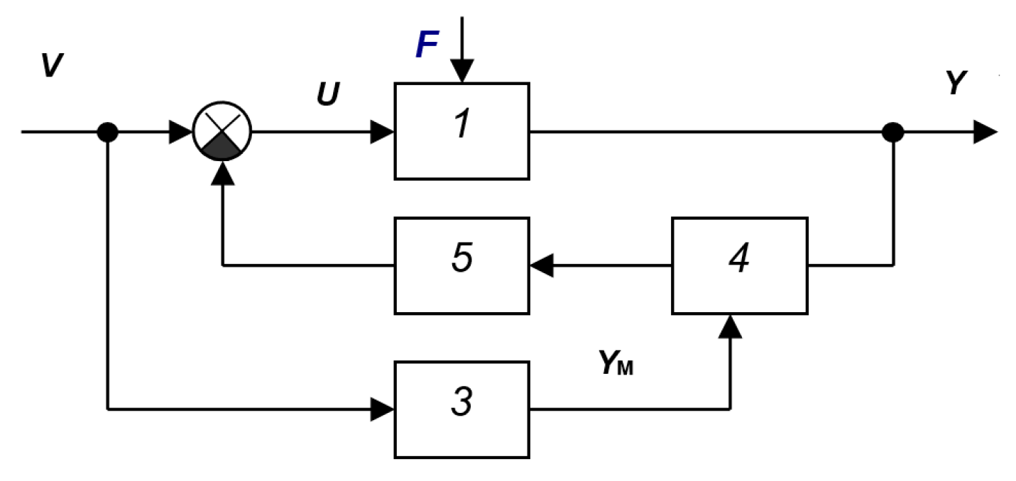
Passive systems are systems with reduced sensitivity to external influences on the parameters of the object, i.e., robust systems. As an example, consider the system in Figure A1 [33]. Similar structures are often encountered in the literature. The book [36] presents a similar system, which is shown in Figure A2, and states that it is transformed into an equivalent system, shown in Figure A3, containing the controller elements and the object in the main circuit, and also having an equivalent low-pass filter at the input. In the case of a large coefficient k of amplifier 4, the output signal of the system Y(t) repeats the output signal of the reference model YM(t). In real systems, the value of k is limited by the stability conditions of the system, and the required equality is achieved only approximately.
Figure A1.
SAS [33]: 1—object, 2—feedback controller, 3—reference model of a locked-loop system.
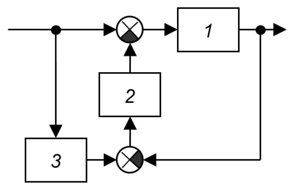
Figure A2.
SAS [36]: 1—object, 2—controller, 3—reference model (locked system), 4—high-gain amplifier implementing deep feedback.
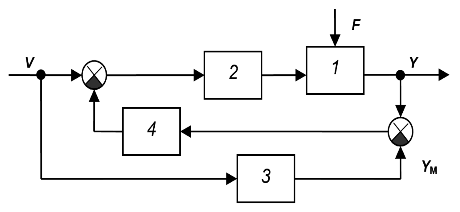
Figure A3.
Equivalent circuit of the SAS according to Figure 2 [36]: 1—control object, 2—controller, 3—reference model (closed system), 4—amplifier with a large coefficient, 5—exact copy of the amplifier with a large coefficient 4.
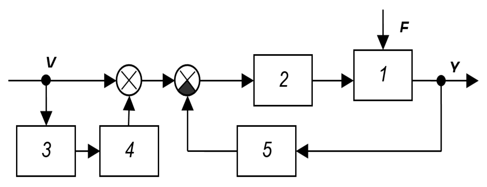
The main drawback of such systems is that with a zero input signal, the adaptation loop is practically meaningless. This structure is ineffective as a stabilizing system. For such a structure to be effective, the loop composed of the main loop elements must be highly responsive. If this is achieved, then the branch connected to the input signal is unnecessary; it merely filters the reference signal. If this fails, then this branch will not improve the situation. The problem is that this loop contains one non-stationary element (object), while the others remain constant. Therefore, the loop’s properties are not adaptive.
The adaptive properties of an equivalent filter connected between the setpoint signal and the adder are insignificant, as they merely change the signal type of the prescribed value for the plant’s output variable, while the stability and quality of the primary control loop remains unchecked and is not corrected by the adaptive loop. In other words, if the loop can become unstable when the plant’s parameters change, then an input filter does not solve the problem. If, however, this problem of maintaining loop stability can be solved, then an input filter is unnecessary. Figure A3, Figure A4, Figure A5, Figure A6, Figure A7, Figure A8, Figure A9, Figure A10, Figure A11, Figure A12, Figure A13, Figure A14, Figure A15, Figure A16, Figure A17, Figure A18, Figure A19, Figure A20, Figure A21, Figure A22, Figure A23 and Figure A24 show examples of such systems from the literature. The aforementioned structural features can be found in all of these examples. The mathematical model of the plant is not directly refined during system operation.
In the system of Figure A24, block 4 multiplies the output signal by its model and averages the result; the result is stated to be equal to the derivative of this functional with respect to the control u(t). However, based on the structural diagram, the system shown in Figure A25 should be classified as an input-dependent system, since in the case of a constant signal v(t) (stabilization system), element 3 cannot perform its functions; therefore, such a system will not exhibit adaptive properties in this mode.
Figure A4.
SAS from the book [37]: 1—object, 2—controller, 3—reference model, 4—converting and executing device.
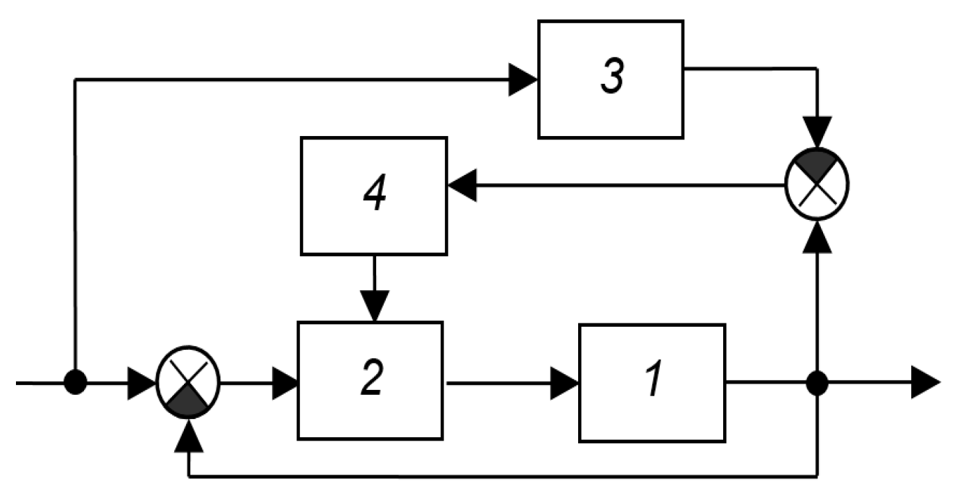
Figure A5.
SAS from the book [37]: 1—object, 2—regulator, 3—adapter.
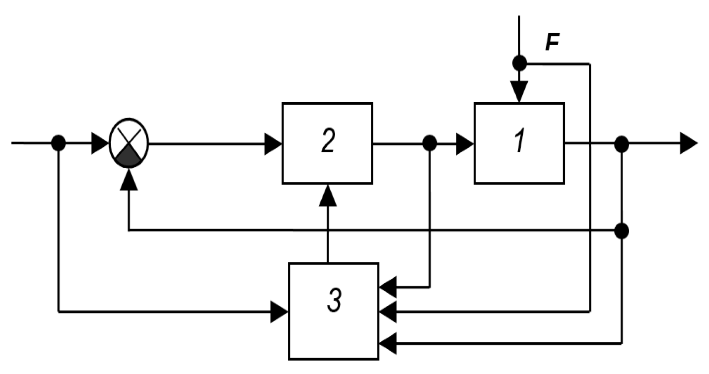
Figure A6.
SAS from the book [28]: 1—object, 2—regulator, 3—model.
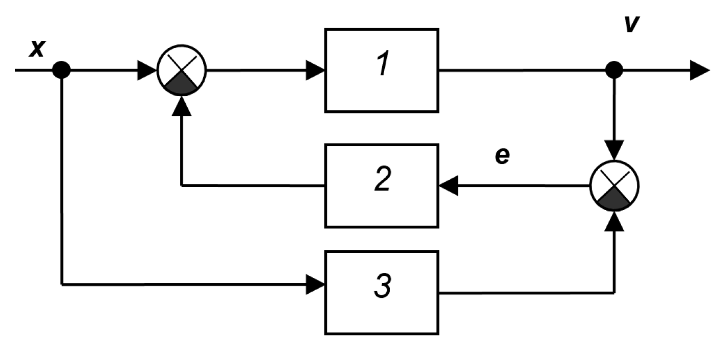
Figure A7.
SAS from the book [28]: 1—object, 2—synthesizer, 3—automatic optimizer, 4—computing device.
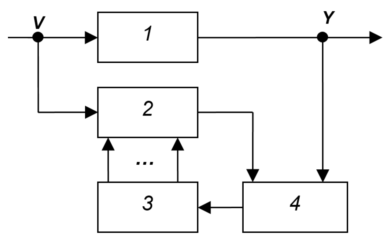
Figure A8.
SAS from the book [28]: 1—object, 2—computing device, 3—synthesizer.
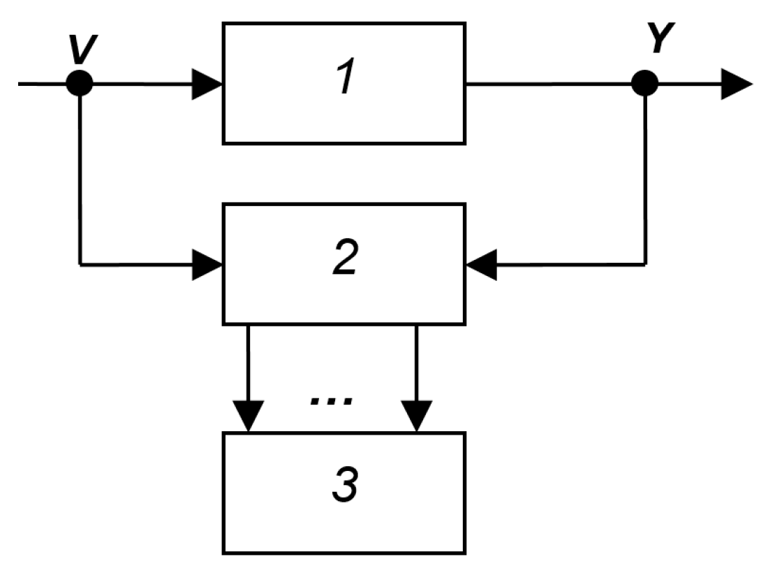
Figure A9.
SAS from the book [28]: 1—object, 2—synthesizer, 3—automatic optimizer, 4—computing device.
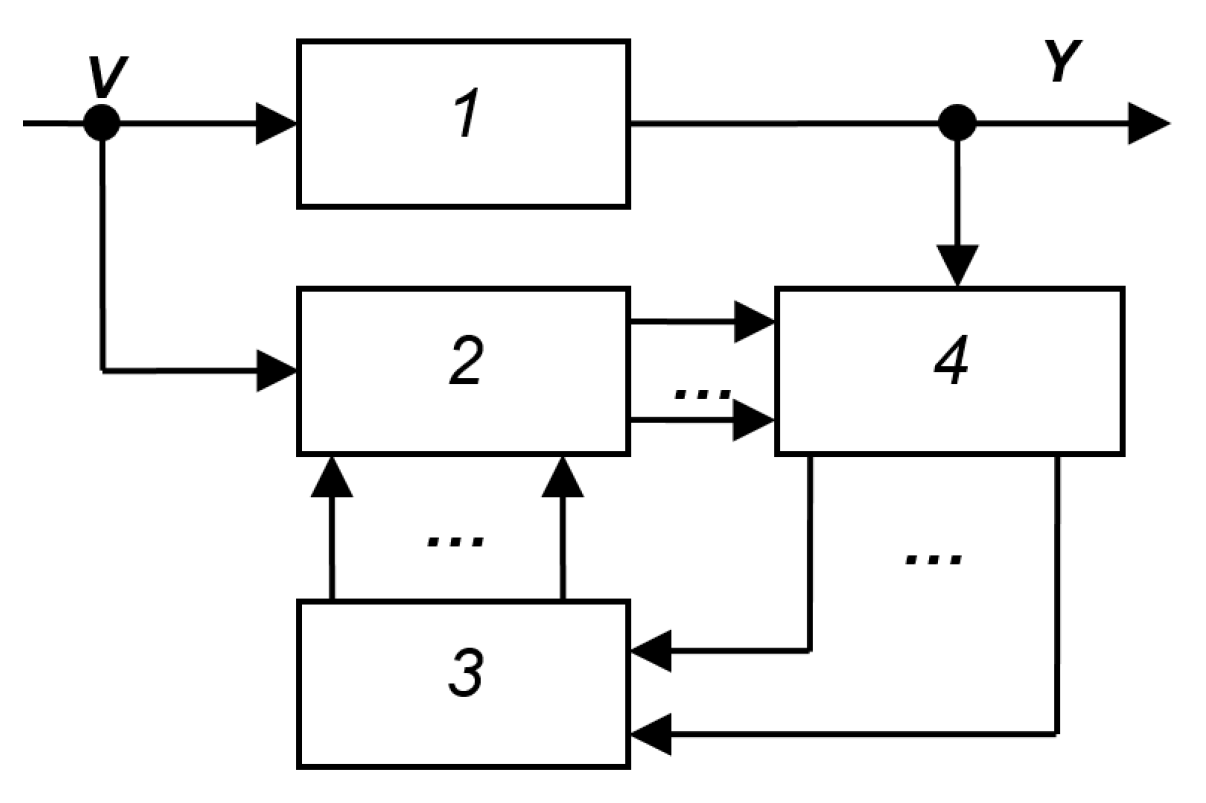
Figure A10.
SAS from the book [2]: 1—control object, 2—regulator, 3—self-tuning device.
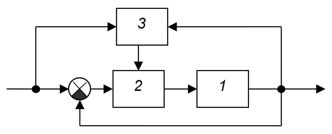
Figure A11.
SAS from the book [29]: 1—object, 2—controller, 3—self-tuning device, 4—transfer function of the control object.
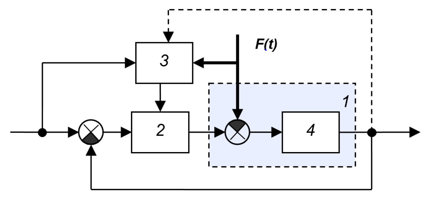
Figure A12.
SNS from the book [29]: 1—object, 2—regulator, 3—locked-loop system model, 4—self-tuning device.
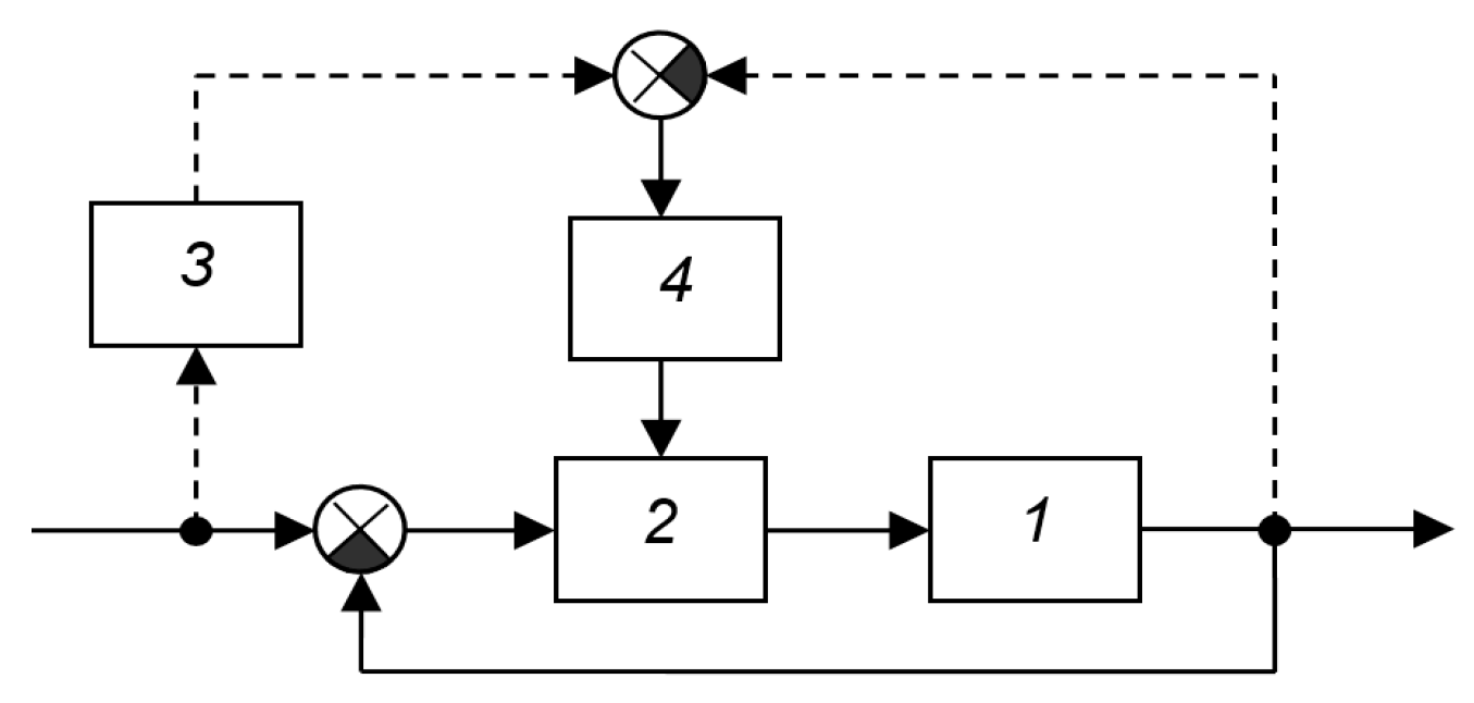
Figure A13.
SAS from the book [29]: 1—object, 2—controller, 3—locked-loop system model, 4—self-tuning device, 5—main (non-unit) feedback.
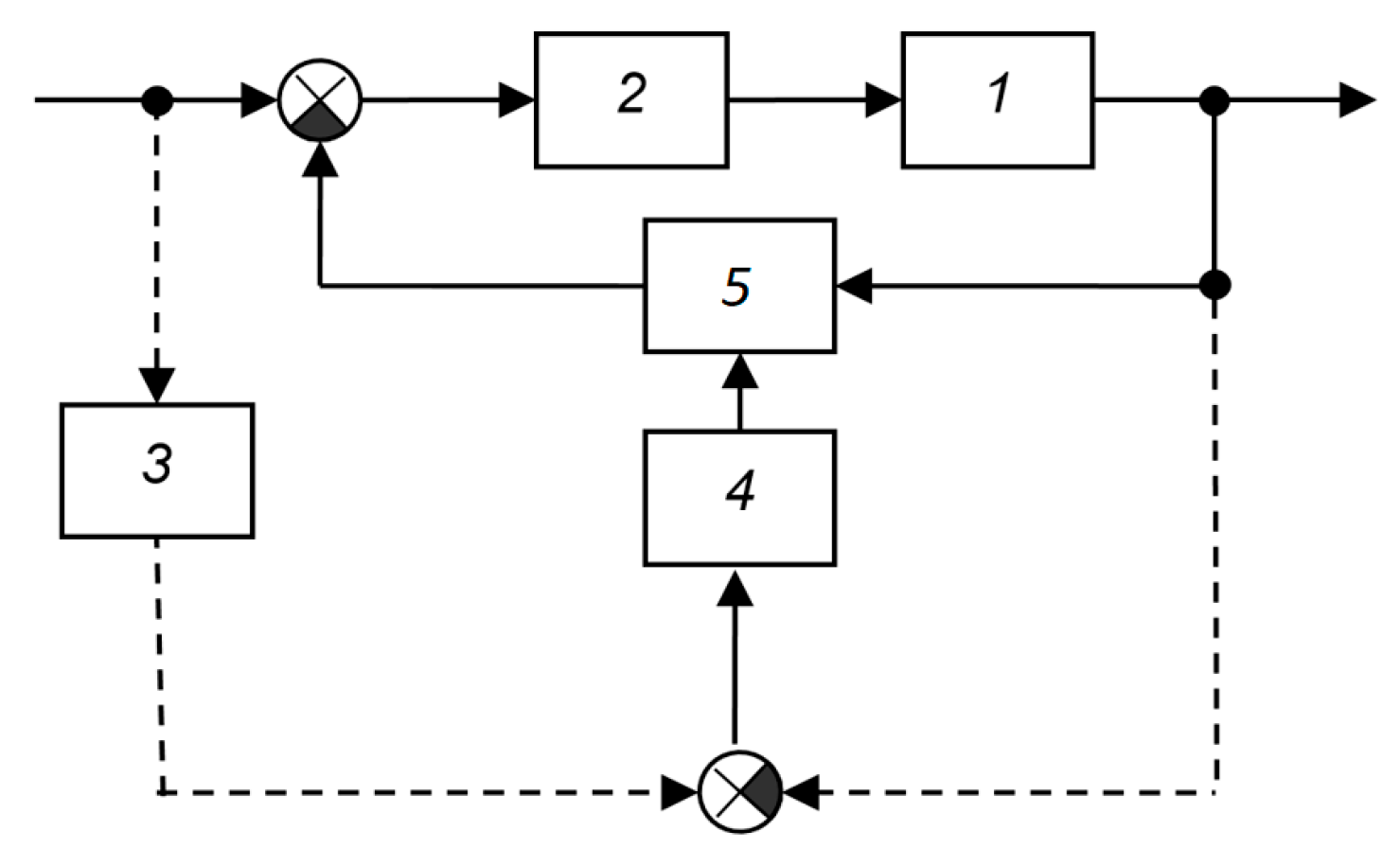
Figure A14.
SAS from the book [29]: 1—object, 2—regulator, 3—characteristics analyzer, 4—self-tuning device.
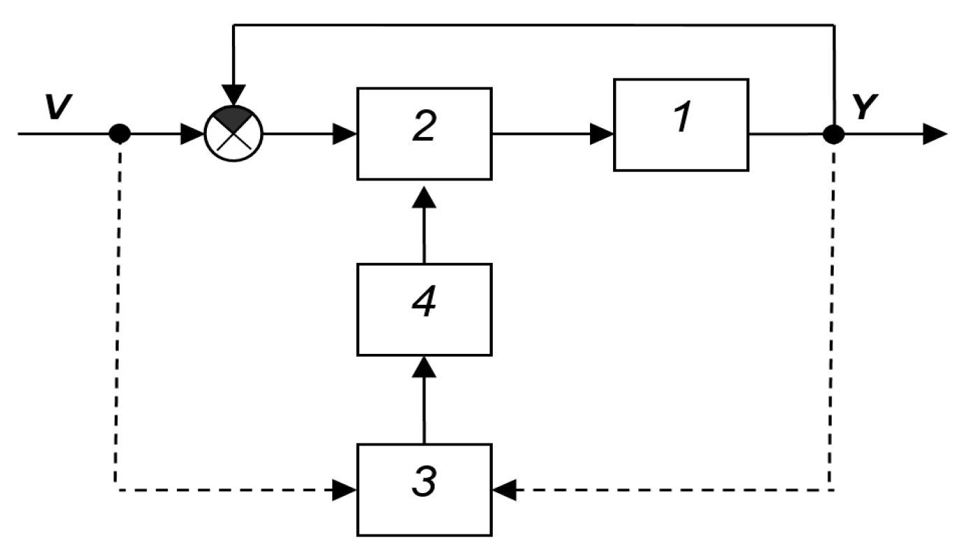
Figure A15.
SAS from the book [38]: 1—object, 2—controlled regulator, 3—computing device, 4—correlator, 5—device for calculating the optimal model of the object, 6—unit for evaluating the real model of the object, 7—comparison device, 8—control device.
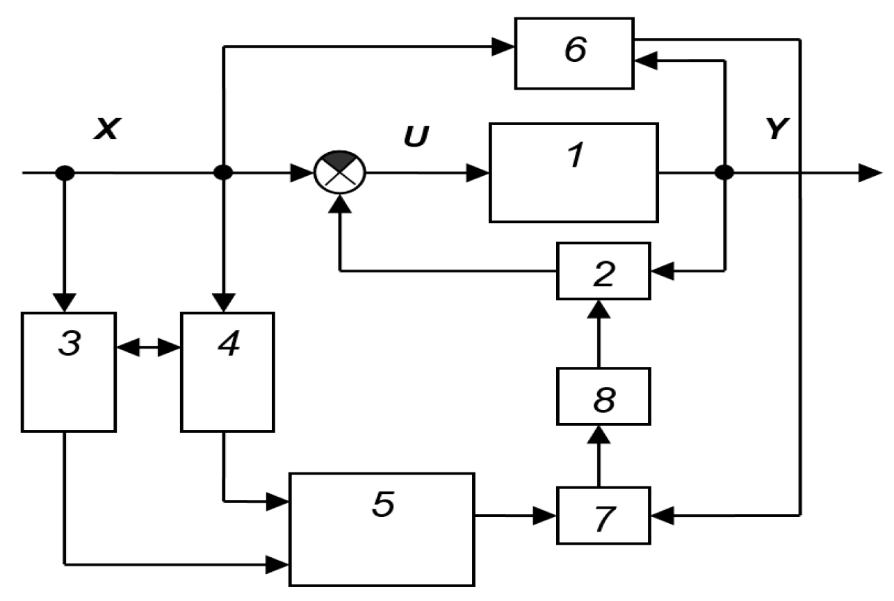
Figure A16.
SAS from the book [37]: 1—object, 2—regulator, 3—reference model, 4—self-tuning device.
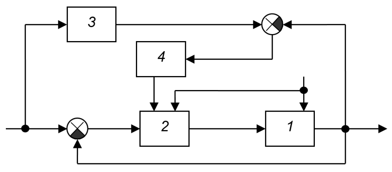
Figure A17.
SAS from the book [39]: 1—object, 2—controller, 3—reference model, 4—computing device, 5—executive body.
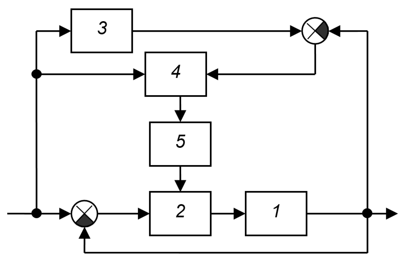
Figure A18.
SAS from the book [39]: 1—object and controller, 2—controller in feedback, 3—reference model (closed system).
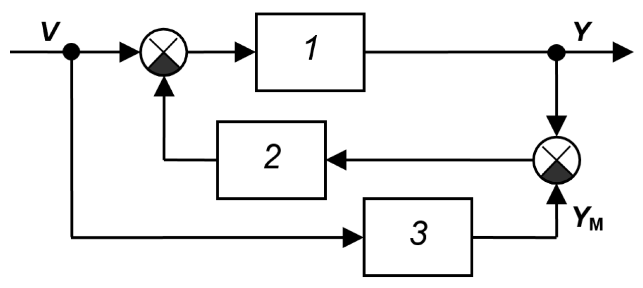
Figure A19.
SAS from the book [39]: 1—object and controller, 2—controller in feedback (with a large coefficient), 3—element with a transfer function equal to the product of the transfer functions of elements 2 and 3 in the previous figure.
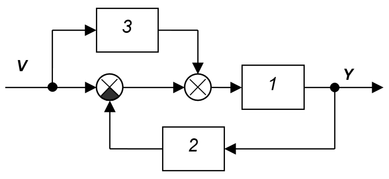
Figure A20.
SAS from the book [40]: 1—object, 2—controller, 3—characteristic analyzer.
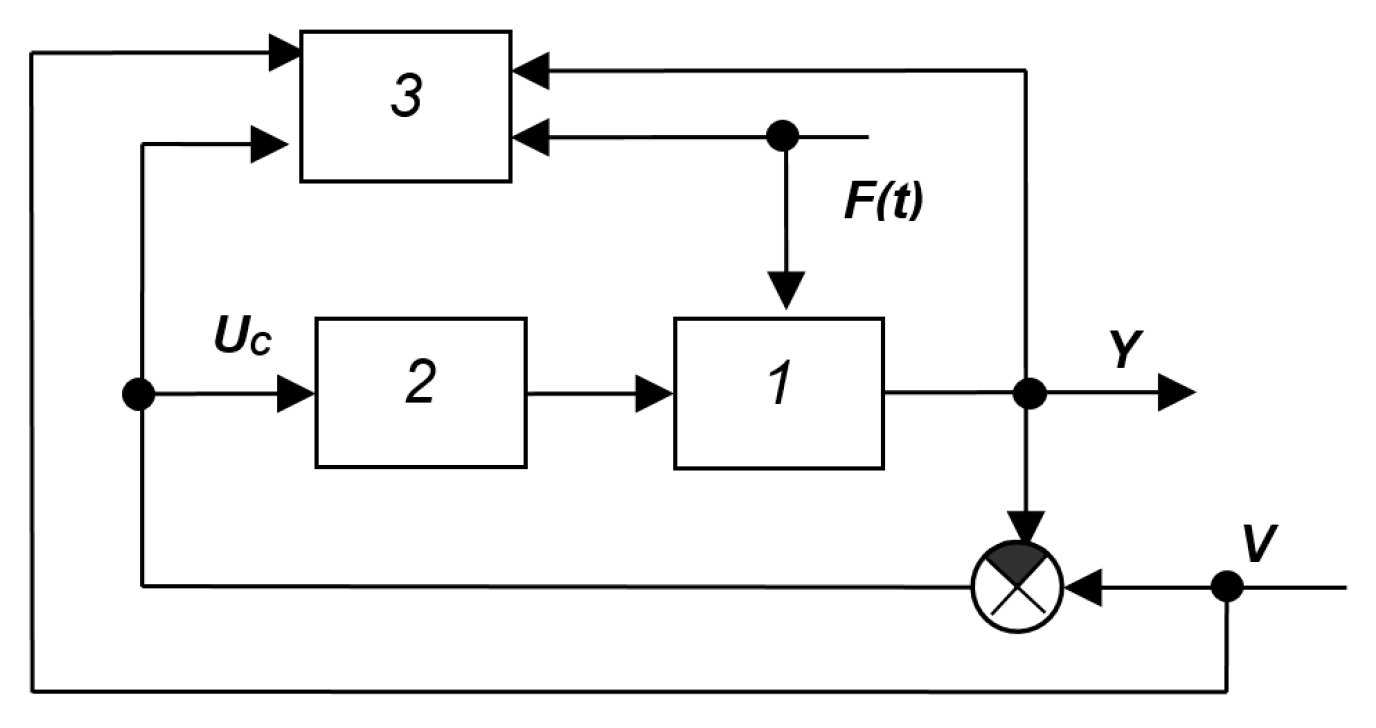
Figure A21.
SAS from the book [39]: 1—object (unknown delay), 2, 3—amplifiers, 4—device with variable delay, 5—multiplier, 6—integrator, 7—regulator, 8—correlator.
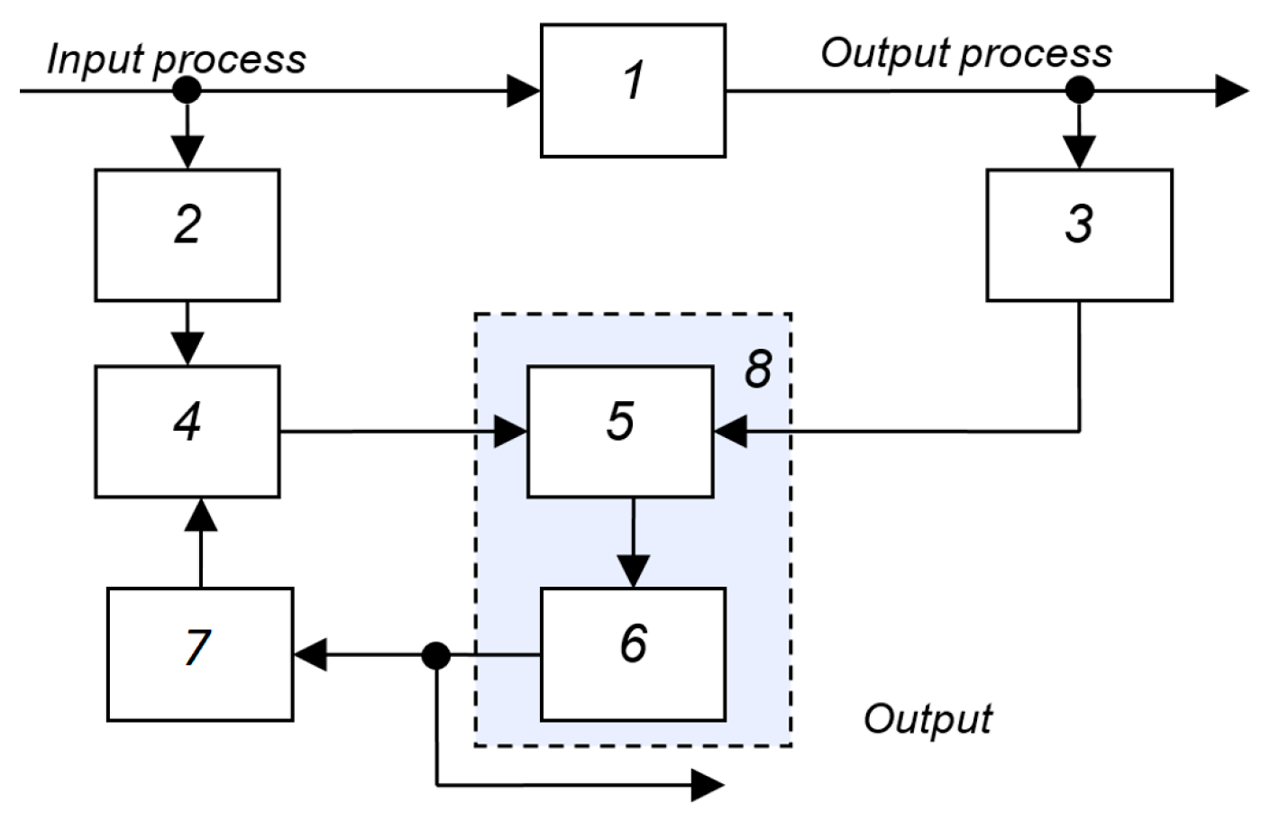
Figure A22.
SAS from the book [36]: 1—external signal analyzer, 2—calculator.
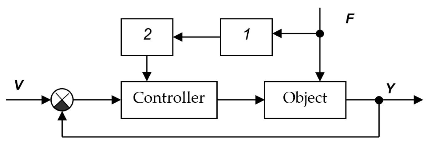
Figure A23.
SAS from the book [36]: 1—object, 2—regulator, 3—correcting and computing device, 4—desired model of the direct contour, 5—signal analyzer, 6—calculator.
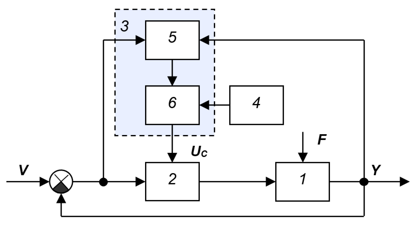
Figure A24.
Structural diagram of a self-tuning model from the book [28]: 1—object, 2—subtractor, 3—dynamic model of the object, 4—block for determining the derivative of the functional Q(Yi) with respect to control, 5—integrator.
Systems without direct identification of the object model
Systems with stabilization of the properties of the main automatic control loop can be classified as a separate class. In such systems, the properties of the dynamic model of the object are not explicitly defined. Instead, they determine changes in the quality function or other operating parameters of the closed-loop system as a whole, and modify the controller’s properties so that the quality of this loop is maintained at a preset level or some quality characteristic reaches its extreme value.
The following subsections can be distinguished within this subclass:
1. Extremum tuning systems: (a) with a trial deviation in the form of a signal introduced into the circuit; (b) with a trial deviation of the controller parameters; (c) without deviation.
2. Systems for maintaining a given quality: (a) with self-oscillation; (b) with the introduction of trial oscillations; (c) without oscillations.
3. Structures in the most general blocks without explanation of the operating principle of at least one of them.
In the system of Figure A25 only the most general blocks are shown [28]. The main feature that classifies this system into the specified class is the connection of the input of block 3 with the output of controller 2 and with the output of object 1. If block 3 determines the dynamic characteristics of the object, then the specified structure should be classified into the next class (the third); if this block determines primarily the degree of coincidence of the output signal y(t) with the input signal v(t), then this system belongs to the given class (the second). Figure A26 shows the SAS from the book [29] with switching of the main feedback on the output variable and its speed. Switching is performed discretely. The tuning device analyzes the output signal and its derivative, as well as the differences between the output signal and its derivative and the specified calculated values. If in stabilization mode, when the input signal does not change, i.e., v(t) = const, the self-tuning device cannot fully perform its functions, then on this basis this system should be classified as the first class, i.e., to systems with adaptation to the input signal. Figure A27 shows the SAS from [39] with a variable structure and indirect measurement of disturbances in the compensation circuit.
Figure A25.
SAS [28]: 1—object, 2—regulator, 3—block for determining characteristics and adjustments.
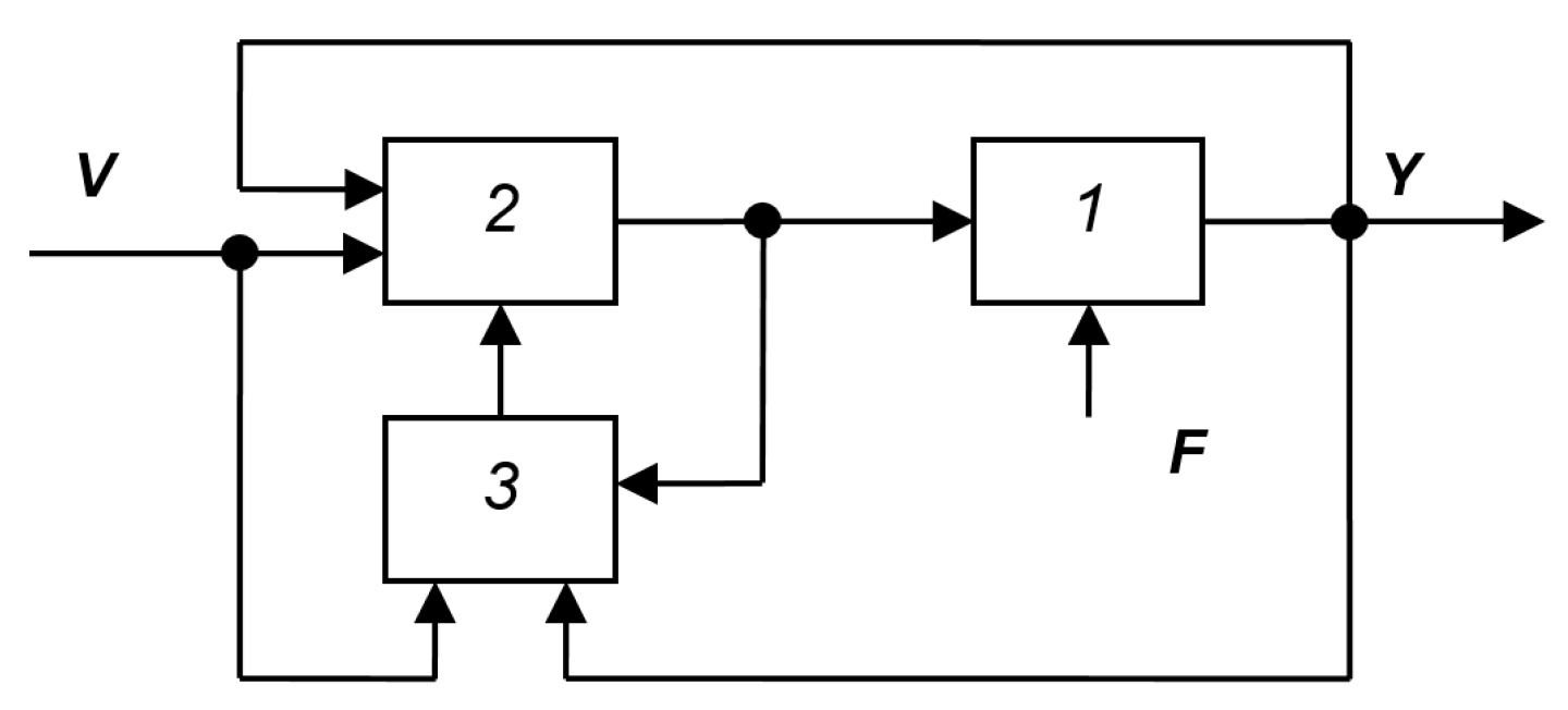
Figure A26.
SAS [29]: 1—object, 2—controller, 3—differentiating element, 4,5—switches, 6—self-tuning device, 7–9—elements of non-unity feedback on the output, 10–12—elements of non-unity feedback on the rate of change in the output.
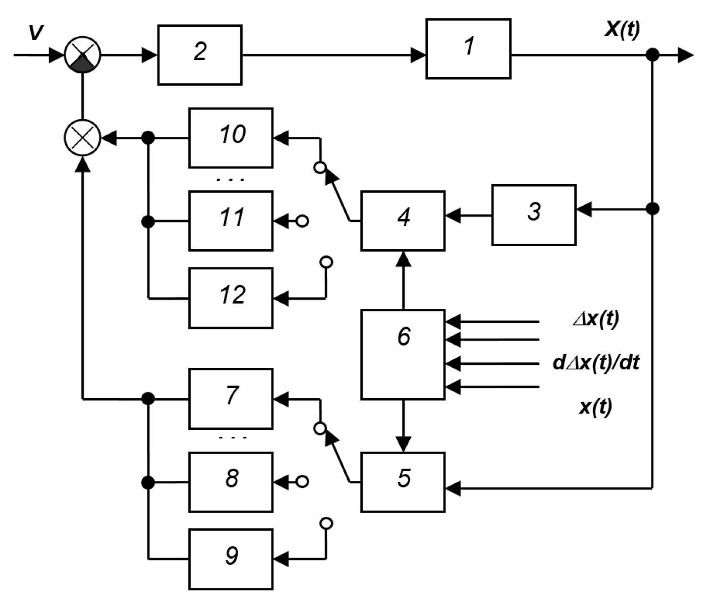
Figure A27.
SAS [39] with a variable structure and indirect measurement of disturbances in the compensation circuit: 1—object, 2—unchangeable part of the regulator, 3,4—changeable parts of the regulator, 5—reference model of the object, 6—compensation channel, 7—control device, 8–9—key, 10—differentiating device.
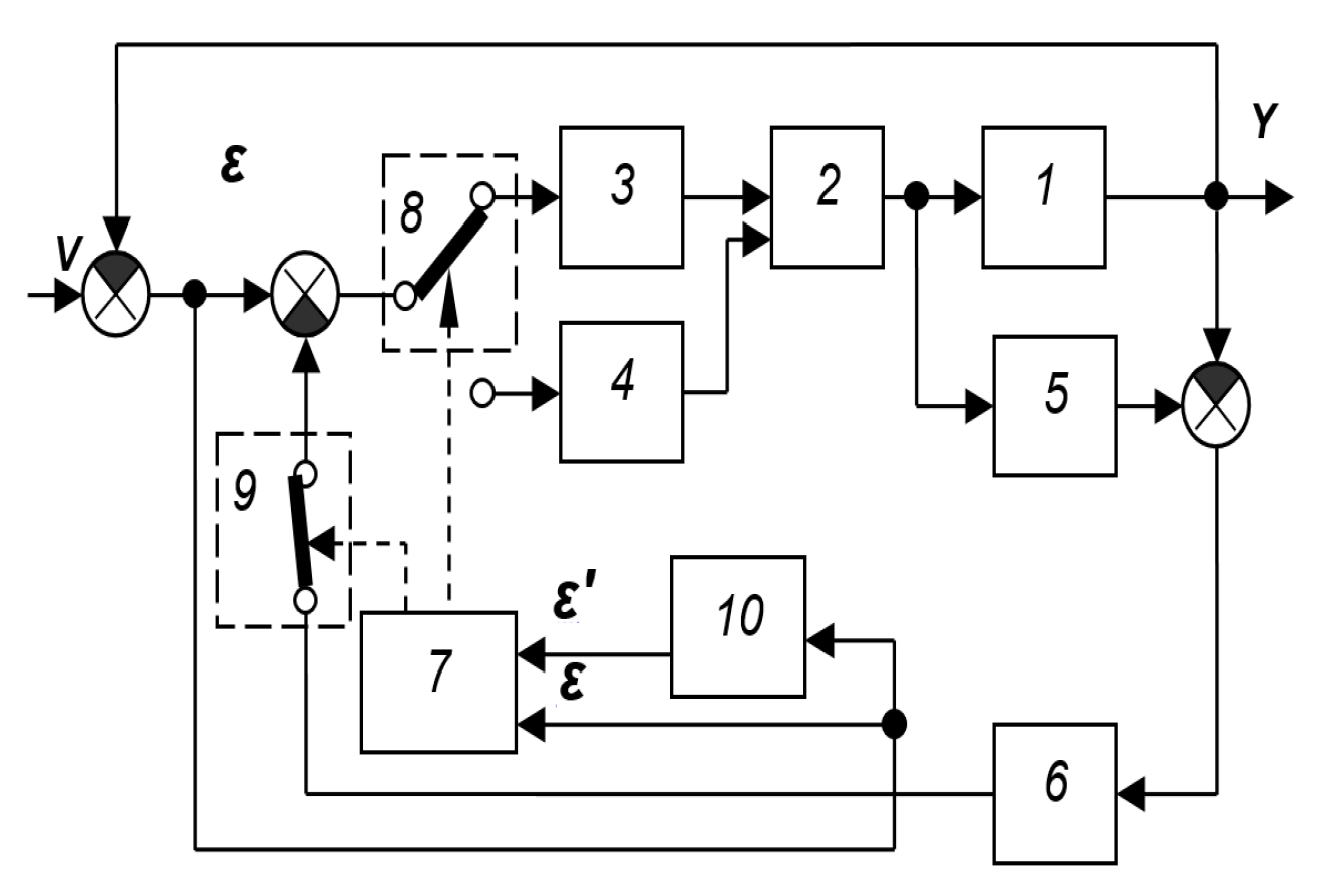
The operating principle of the system is based on the organization of a sliding mode along the switching line S = ε + C ε’. Element 13 is derivating device for calculating the derivative of the error. Element 10 and its connections are not shown in the diagram; only the input signals of element 7—the control error ε and its derivative ε’—are shown.
Figure A28 shows the SAS with parametric feedback from the book [40]. Changes in the parameters of object 4 disrupt the tuning of the system. Elements 5, 6, 7 and 3 serve to compensate for changes in the parameters of object 4. For this purpose, the parameters of the series controller 2 are selected such that, with the initial state of the parameters of the object, small self-oscillations arise in the system around the equilibrium state. Their amplitude is negligibly small from the standpoint of the quality of the system’s functioning, and their frequency is significantly greater than the frequency band of the signal that must be processed by the closed system. The frequency band of filter 5 is selected so as to pass only the fundamental harmonic of the resulting self-oscillations. The rectifier selects the amplitude of these oscillations, and filter 7 smooths the received signal and feeds it to the control input of the adjustable amplifier 3. Thus, elements 3–7 form an additional circuit for stabilizing the amplitude of self-oscillations, and changes in the gain of object 4 are compensated for by inverse changes in the gain of the adjustable amplifier 3. As a result, the overall coefficient of elements 3 and 4 remains constant, ensuring stable operation of the main circuit formed by elements 2–5. The self-oscillation frequency should be 3–4 times greater than the maximum frequency of the input signal spectrum and lie outside the interference frequency spectrum affecting the system. Filter 1 filters the input signal to remove components near the self-oscillation frequency.
The first drawback of this system is the necessity of providing a closed-loop bandwidth much larger than that required to process the useful signal X. In this case, it is necessary to use only a portion of the system’s capabilities, artificially reducing its response time. Thus, the solution to the problem contradicts the stated goal, which is to ensure the largest possible bandwidth and the highest system accuracy with changing object parameters. The second drawback of this system is its narrow scope of application, since it is assumed that achieving stability in the amplitude of self-oscillations is identical to achieving system stability, which is not achieved for all objects. The third drawback of this system is the need to ensure the constancy of not only the amplitude but also the frequency of self-oscillations by changing the gain of element 3. This presupposes high stability of all object parameters except its overall gain, which is rarely achieved. The fourth drawback of such a system is the need for preliminary adjustment of controller 2, which requires detailed knowledge of the mathematical model of object 4 and, consequently, significant preliminary research. The fifth disadvantage of this system is the presence of oscillations in the output signal, which reduces the accuracy of ensuring equality between the input signal X and the output signal Y.
Figure A29 shows SAS with parametric feedback from the book [40]. This system is in many ways similar to the previous one. Changes in the gain of object 2 are compensated by inverse changes in the gain of amplifier 1 in such a way that the resulting gain of the circuit, which includes the object and the controller, is constant. Elements 3–6 serve to detect and automatically adjust the changes in the coefficient. For this purpose, harmonic oscillations Z are introduced into the circuit from generator 3 through the adder, which are partially suppressed by the circuit due to the action of negative feedback, and their remainder is present at the outputs of all elements, including the output of amplifier 1. Filter 4, tuned to the frequency of these oscillations, rectifier 5 and low-pass filter 6, connected in series, detect the amplitude of these oscillations. The magnitude of this amplitude is fed through the adder to the controlled amplifier 1, changing its transmittance so that the amplitude is constant. The signal R of the preliminary tuning of amplifier 1 is fed to the second input of the adder. If only the gain of the object changes, this will lead to a change in the amplitude of the harmonic component of the signal at the output of amplifier 1, but the action of the additional amplitude stabilization circuit, composed of elements 4–6, will change the gain of amplifier 1 such that the value of this amplitude remains unchanged. This will be achieved only by restoring the initial value of the gain of the entire circuit, equal to the product of the gain of object 2 and the gain of amplifier 1. As a result, changes in the gain of object 2 are compensated by inverse changes in the gain of the regulated amplifier 1, the overall gain of the main control path remains unchanged, thereby achieving the additional path in the system.
The main drawback of this system is its insufficient operational accuracy and insufficient self-tuning efficiency. This insufficient accuracy arises from the fact that the system must oscillate during operation. Insufficient tuning efficiency arises from an inadequate relationship between the adjustable parameter (oscillation amplitude) and the actual quality of the system tuning, which is related to the operating frequency bandwidth, control error margin, and system stability. This leads to a third drawback: the need to pre-tune the system using certain additional performance criteria. A fourth drawback is the limited scope of this method, as it is effective only when the only variable parameter of the system is its gain. Therefore, this device cannot provide high speed and high accuracy.
In the system shown in Figure A30, it is proposed to include a system quality assessment device in the system and to ensure that the controller is adjusted to the best quality due to the action of an additional feedback loop formed by a synchronous detector and a coefficient controller [41]. Accuracy is improved by eliminating output fluctuations during operation. Efficiency is improved by using a criterion directly related to the closed-loop system’s performance indicator, which is calculated continuously or periodically during system operation.
Systems with a reference model of the object
Figure A31 shows the SAS from the book [36], which represents a typical system with a reference model of the object. Unlike a system with a reference model, which specifies the response of the entire system as a whole to the input signal v(t), such as the systems in Figure A6 and Figure A16, in this system the reference model specifies the prescribed response of the object to the input, i.e., the control signal u(t). It is easy to see that the operating conditions of this circuit do not require that the reference signal (the prescribed value for the output) v(t) change over time. The adaptation circuit remains operational even if the reference is zero (as in the case of tracking systems), and the operation of the entire system is aimed at processing non-zero initial conditions and (or) the action of the interference F(t).
Figure A28.
SAS with parametric feedback from [40]: 1—filter, 2—controller, 3—adjustable amplifier, 4—non-stationary object, 5—filter, 6—rectifier, 7—filter.
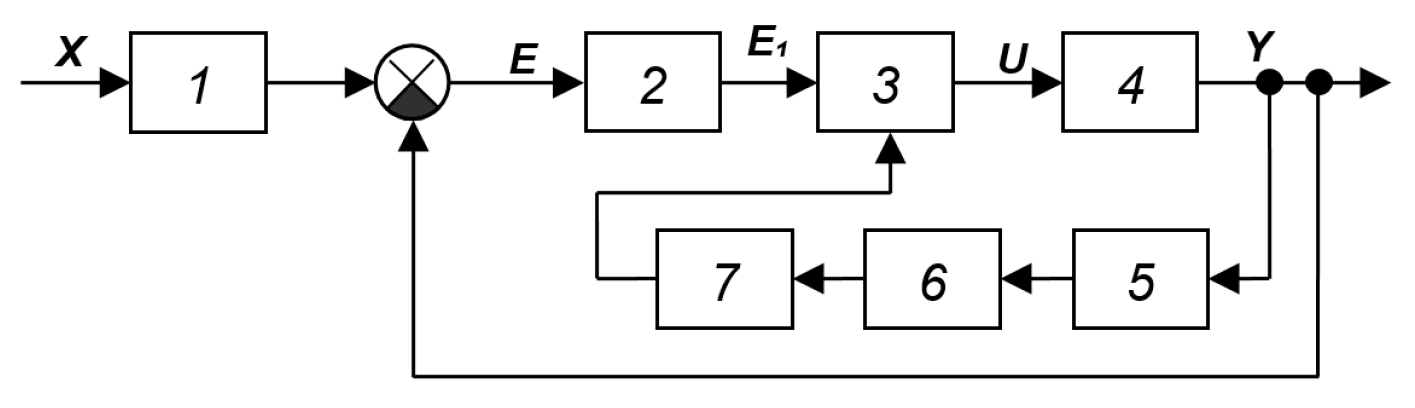
Figure A29.
SAS with parametric feedback from [40]: 1—controlled amplifier, 2—object, 3—generator, 4—filter, 5—rectifier, 6—filter.
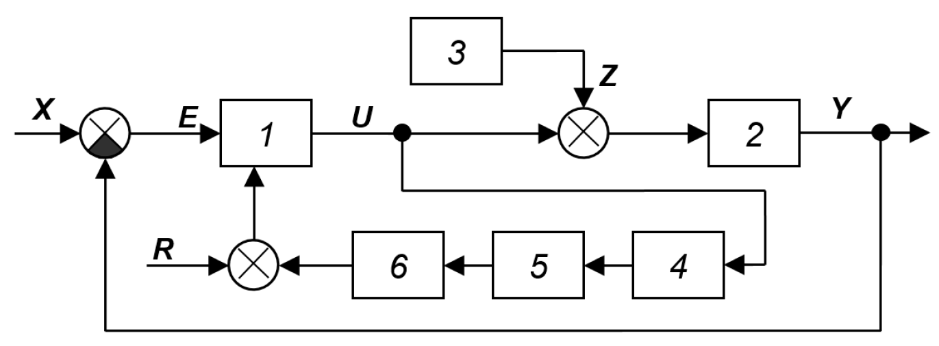
Figure A30.
SAS with gain deviation: 1—controlled amplifier, 2—object, 3—generator, 4—system quality assessment device, 5—synchronous detector, 6—gain controller [41].
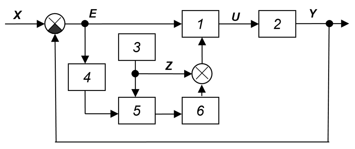
The task of the self-tuning circuits is to calculate the current dynamic characteristics of object 1, changing under the influence of an unknown and unpredictable external influence F, analyzer 6 determines the parameters of the inverse model and enters them into calculator 7.
The reference model in the system shown in Figure A31 is implicit. It does not take into account the effect F(t), but only the input signal (control) u(t). The plant’s output signal Y(t) should be the same as it would be in the absence of the disturbance. The difference between the actual output signal and the output signal of the plant’s reference model constitutes a control error for the adaptation loop. Feedback from this loop acts on the controller, changing its parameters so that the plant’s output signal is as close as possible to the model’s output signal. The advantage of this technical solution compared to the structure in Figure A1 and Figure A16 is its versatility (the dependence on the dynamic activity of the signal V is eliminated, i.e., it can be variable or constant, including zero). The implementation of this circuit requires preliminary identification of the object in order to determine its characteristic or expected mathematical model, which is implemented by block 5. For this model, controller 2 is calculated, consisting of a fixed part 3 and a variable part 4. It is assumed that the variable part of the controller can change under the influence of the correction signal UC(t), and it is inverse with respect to the object model. In other words, the product of the transfer functions of elements 4 and 1 is equal to unity over as wide a frequency range as possible. This requirement is never achieved in practice, but it can be approximated within a certain upper-bound frequency range. Within this range, the controller should be calculated and implemented under the assumption that, beyond this range, any deviation of the specified product of the transfer functions from unity (or downwards) has an insignificant effect on the dynamic and static characteristics of the closed-loop control.
SAS schemes from the book [28], shown in Figure A32 and Figure A33, could be conditionally classified as systems with adaptation based on the input signal. But, since this connection is shown in both cases by a dotted line, the conclusion about its optionality is correct. Therefore, the circuit in Figure A32 can be interpreted as a multichannel system with a controller in the feedback, and the circuit in Figure A33 is its development, a special case or clarification, in which the controller, separated from the automatic optimizer, is explicitly identified. The output signal of the controller is a vector of control actions U(t), the vector of output signals is also analyzed. In both structures, apparently, the model of the object is not defined, but a certain functional Q(Yi) is determined, known for the optimal operation of the system. Adaptive feedback attempts to reduce the deviation of the calculated value of this functional from its prescribed value to zero. The requirement that the functional of the output signal vector match some predetermined form is analogous to implicitly defining a mathematical model of the object’s output based on its input vector. Therefore, the two specified structures can be classified in this class.
Figure A31.
SAS [36]: 1—object, 2—controller, 3—desired model of the direct loop, 4—inverse model of the control object, 5—internal signal analyzer, 6—calculator, 7—correcting device.
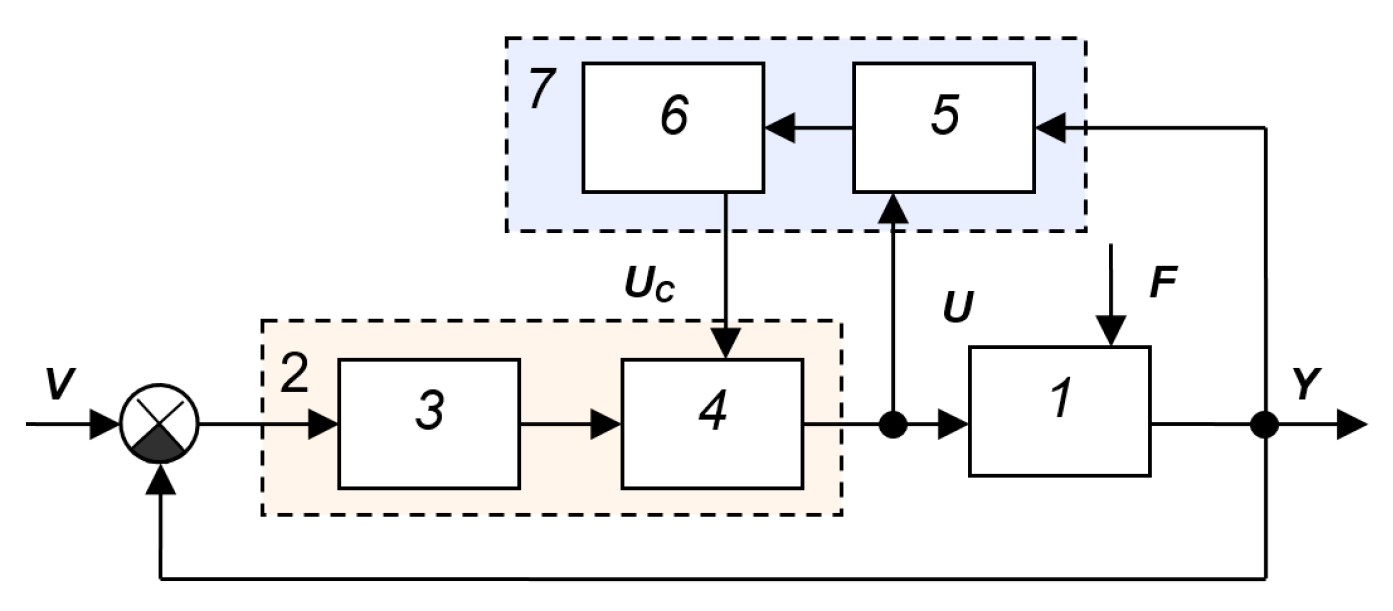
Figure A32.
SAS [28]: 1—object, 2—block for defining the functional Q(Yi), the variation in which should be reduced to zero, 3—automatic optimizer.
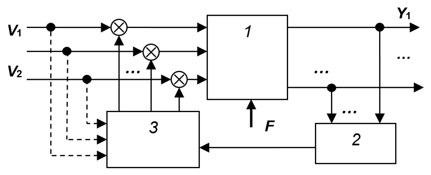
Figure A33.
SAS [28]: 1—object, 2—block for determining the functional Q(Yi), the variation in which should be reduced to zero, 3—automatic optimizer, 4—K-dimensional controller.
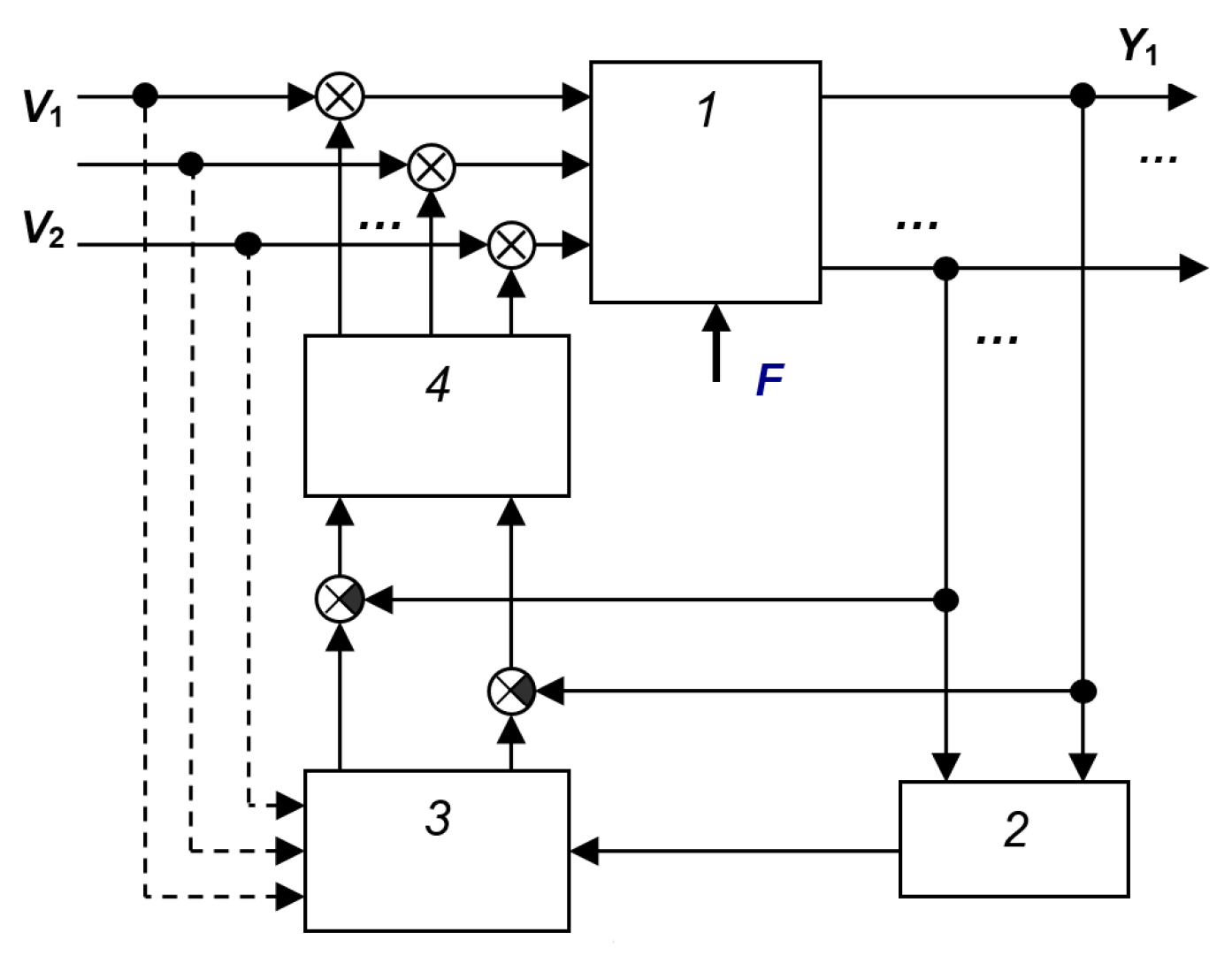
A generalized and less detailed structural diagram of such an SAS [39] is shown in Figure A34. Such overly general diagrams are useful only as a starting point for the developer or for explaining the general operating principles of adaptive systems for educational purposes. For their practical implementation, it is necessary to detail all blocks (except the object), the operation of which is not sufficiently clear from the name. Figure A35 shows the SAS from the article [42]. The device is designed to adapt the operation of the system based on an object with a changing parameter of its mathematical model. Figure A36 shows an adaptive SAS with the reference model from the book [39]. Its operating principle is similar: the output signal of the reference model 3 is compared with the output signal of the real object 6, the difference is fed into the circuit through the correction device 4. Unlike the system shown in Figure A34, in this system the signal from the output of the correction device is transmitted through the adder not to the output of the controller, but to its input. It is also possible to measure the disturbance F and, based on this, generate a compensating effect in the circuit. If we define a disturbance as an effect that cannot be measured, then the presence of the compensating circuit 7 is irrelevant.
Figure A37 shows the SAS with the reference model from the article [43], which describes a technique for detecting changes in the dynamic characteristics of a process. The method is based on real-time calculations of process components and comparison of the result with the values obtained during the process.
Figure A34.
SNS from [39].
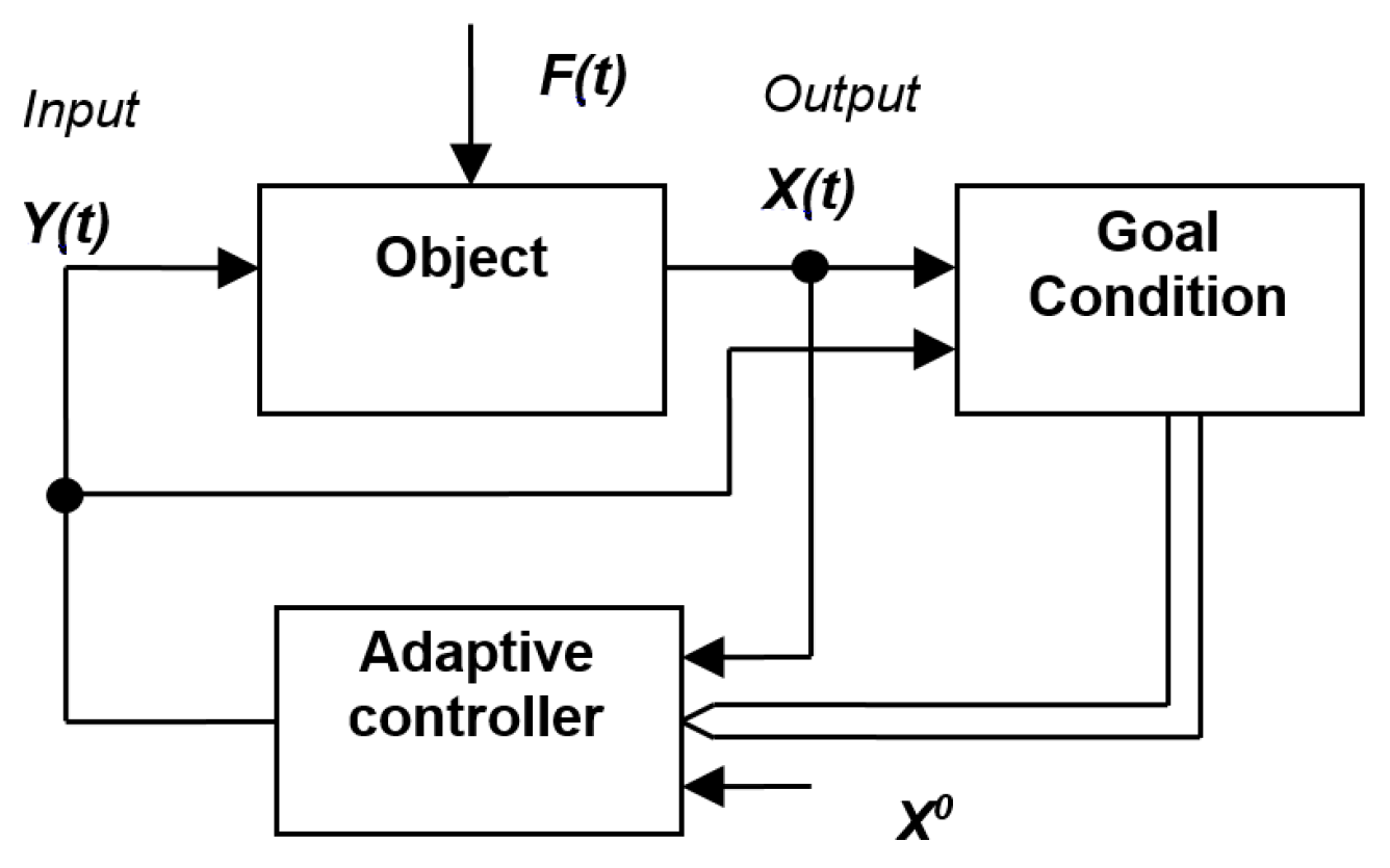
Figure A35.
SAS with a reference model from the book [43]: 1—object, 2—controller, 3—reference model of the object, 4—differentiating filter, 5—block for calculating the sum with coefficients, 6—nonlinear converter, 7—adaptive controller.
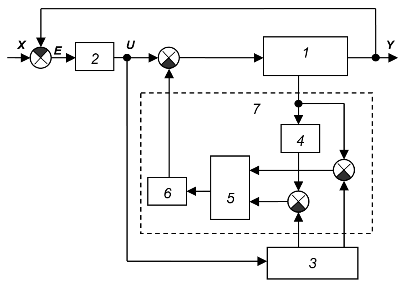
Figure A36.
SAS with a reference model [39]: 1—object, 2—controller, 3—reference model, 4—correction device, 5—transfer function of the object for control, 6—transfer function of the object for disturbance, 7—transfer function of the compensating circuit.
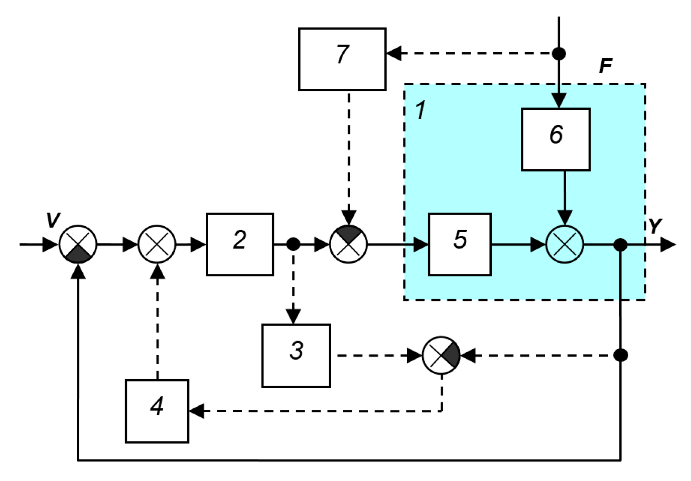
Figure A37.
SAS with the reference model from the article [43]: 1—object, 2—controller, 3—object model, 4—controller model, 5—object transfer function, 6—simulated control loop, 7—physical (real) control loop.
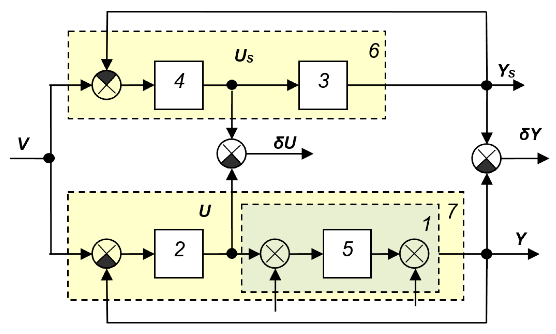
Structures of systems with a reference model also appear in fairly recent scientific publications, such as [44,45,46]. Examples of such structures are shown in Figure A38 and Figure A39. The disadvantages of these systems are the same as those of the systems of this class considered above.
Systems with object model identifier
This class includes systems containing a computing device that, by virtue of its structure and/or operating algorithm, identifies the mathematical model of the object. In other words, during the device’s operation, and at the same time that the primary feedback loop ensures the output value is equal to its prescribed value, the secondary loop ensures stability (and optimal tuning) of this loop by refining the parameters of the object model, which can change slowly over time. Naturally, the rate of change in the object model parameters must be significantly lower than the rate of transient processes in the system, but this observation is true for all adaptive systems except those that provide feedback on the full state vector of the object.
Figure A38.
Another variant of the adaptive system with reference model from [44].
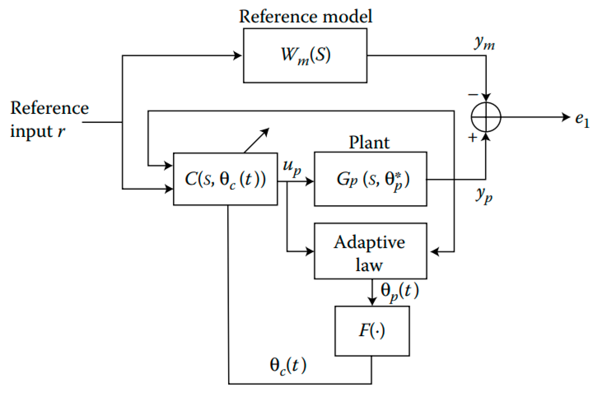
Figure A39.
Adaptive system with reference model [44].
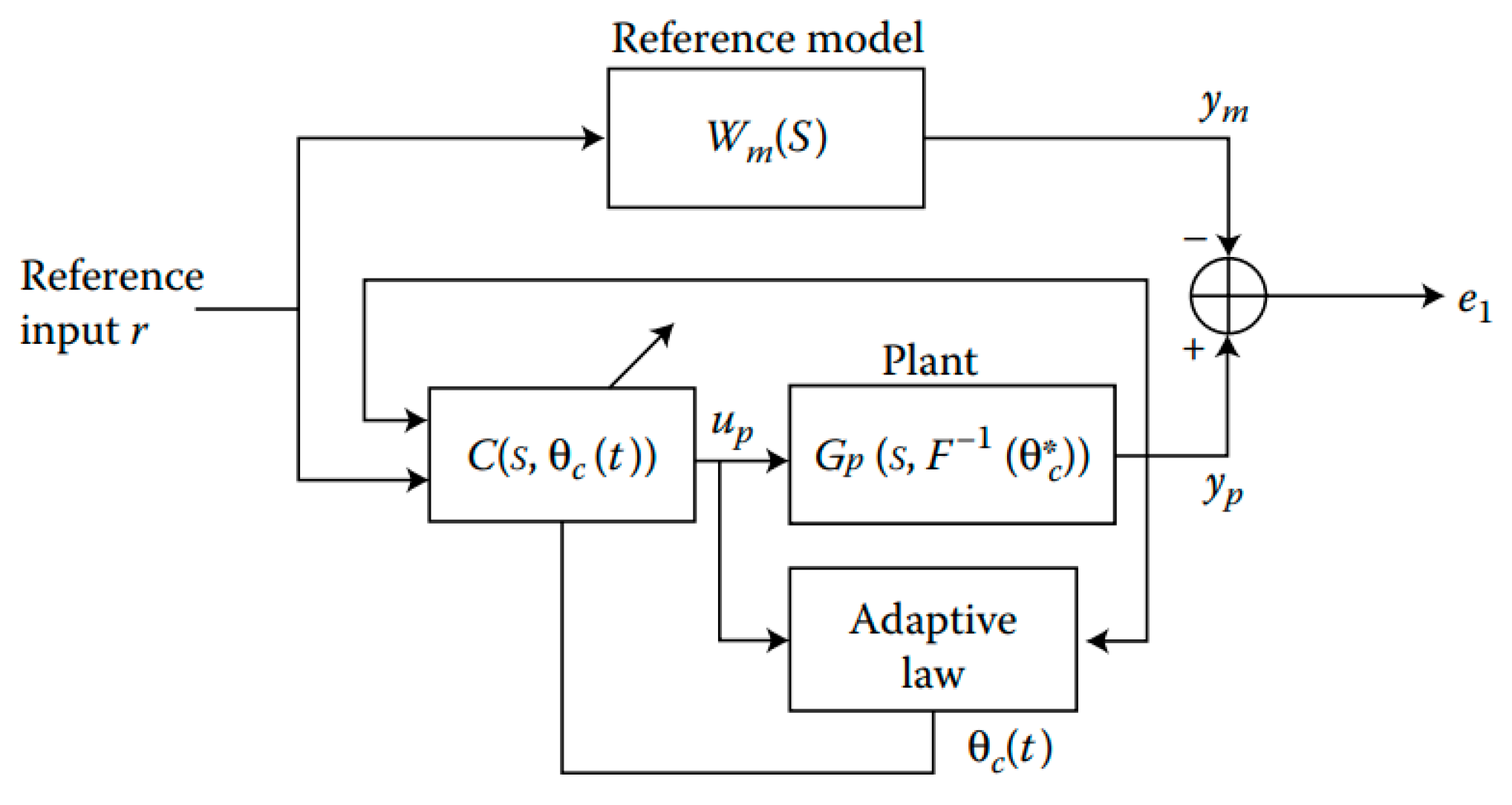
Figure A40 shows the most general structure of an STS from [39]. The principle of its operation is clear from the figure. The identification block, analyzing the signals arriving at the input of the object and coming from its output, determines a mathematical model that defines the relationship between them. Note that, since the object is a real device, not every mathematical relationship may correspond to its mathematical model. The mathematical model is found in the class of admissible functions. The more information about the object, the simpler the structure and the more accurate the operation of the identification block. The self-tuning block must receive information about the current model of the object and, based on this, act on the regulator in such a way as to change its parameters in the desired direction and ensure the best (or acceptable) parameters of the main control loop. The disadvantage of the structure of Figure A38 is only its incompleteness. Other structural diagrams, to a greater or lesser degree of detail, reveal the operating principle of these two blocks. For example, the circuit shown in Figure A41 [37] is even less detailed, but places the system in the same class. The circuit shown in Figure A42 [28] differs from the circuit in Figure A41 by the presence of a connection between the system’s input signal and the identification unit. For a stabilization system (if the input signal does not change), the presence of this connection is unimportant, but if the operating principle of the identification unit is based primarily on the analysis of this signal, then this system should be classified as a system with adaptation based on the input signal. The same is true for the system shown in Figure A43 [28].
Figure A40.
SAS from [39].
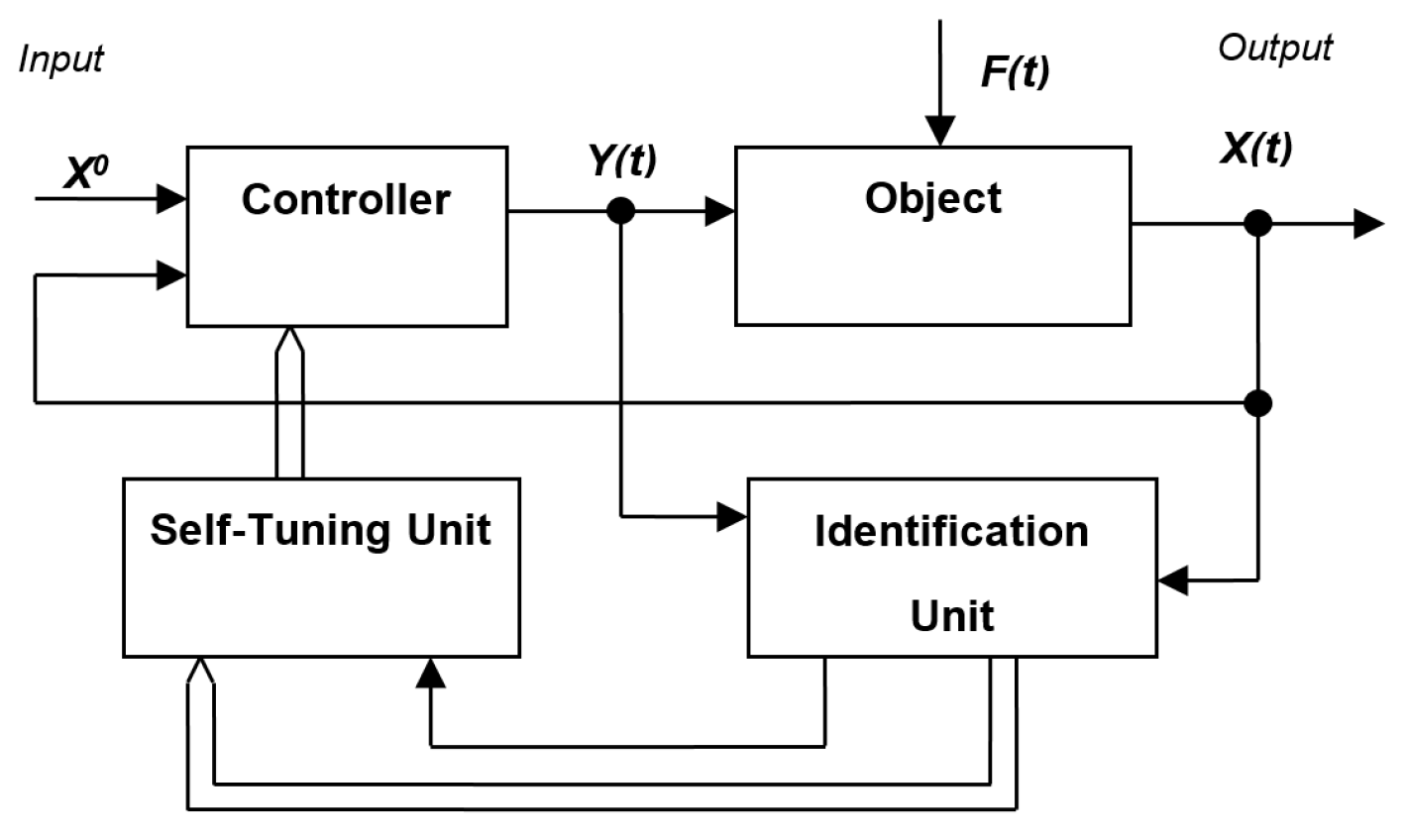
Figure A41.
SAS with identifier from [37]: 1—object, 2—controller, 3—identifier.
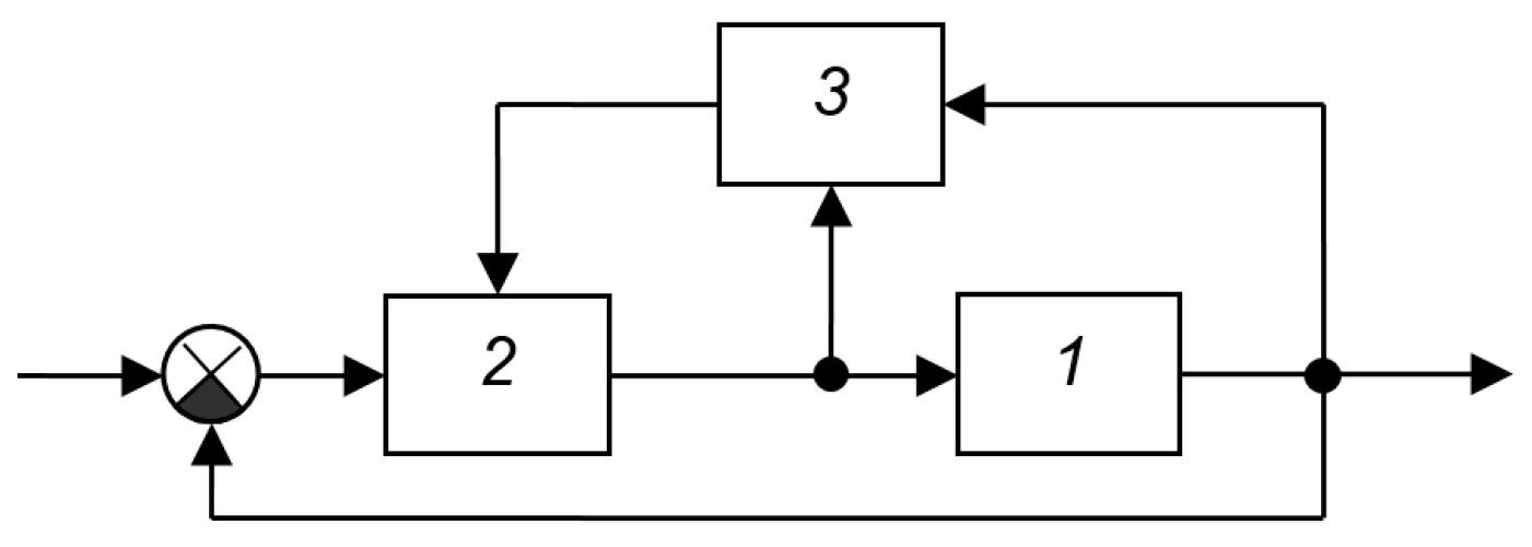
Figure A42.
SAS from [28]: 1—object, 2—control device (regulator), 3—block for determining characteristics and settings, 4—model.
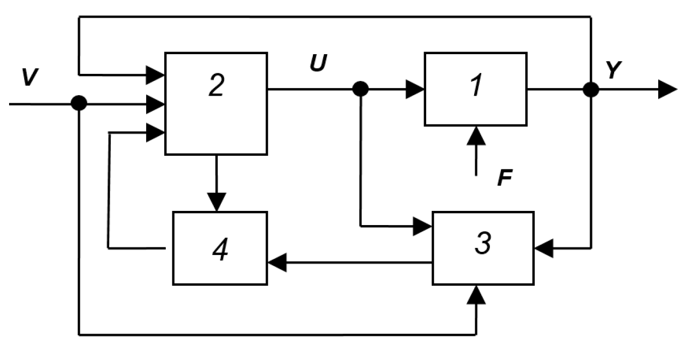
The SAS block diagram, shown in Figure A44 [28], contains more detail and reveals the specific principle of object identification. This principle is based on modeling the object’s response using a model compiled from a priori or experimentally accumulated information about the object. The subtractor determines the difference between the output signal of the real object and the output signal of the virtual model. This difference, via a tuning unit, controls the model’s parameters, bringing them into closer conformity with the real object. The computing device, based on the refined information received about the model, the controller, acting on it through the actuator. When using digital controllers based on microprocessors with an ADC at the input and a DAC at the output, the division into blocks is purely arbitrary: all functions of the controller, identification block, and self-tuning block are performed by a single digital device (microcontroller). In this case, no special actuator is required; knowledge of the calculated controller is sufficient for its implementation using signals calculated numerically according to the required mathematical model of the controller and according to the signals from the object’s output determined using the ADC. The generator of the prescribed value v(t) can also be part of this digital device. Therefore, in the structure in Figure A42, the most important part is the loop with the tracking model consisting of elements 3 and 4.
The structure shown implies that only one analyzing device (the subtractor) analyzes the results of changes in the object’s parameters, while there may be multiple parameters being changed. If only one parameter changes and if its effect on the output signal is unambiguous, then the described operating principle can be implemented. However, even in this case, there are obstacles to its effective operation, since the real object is also affected by disturbances (otherwise known as noise), while these do not affect the model, since disturbances are effects that cannot be measured. The loop shown in Figure A45 from the book [28] differs from the previous one only in that it has a pre-filter, and the controller is divided into two blocks—a feedback controller and a converter in the forward branch. From the standpoint of ensuring the required properties of the main circuit, the series-connected elements 2 and 5 constitute a single controller; as a rule, a fundamentally better effect is not achieved by dividing them. The filter included at the system input does not change the system’s stability, but only corrects the spectrum of the input action. Therefore, from the standpoint of the usefulness of the considered structures for the development of SAS, these circuits (Figure A44 and Figure A45) are identical.
Figure A43.
Structural diagram of the closed identification method from [28]: 1—object, 2—model, 3—computing device.
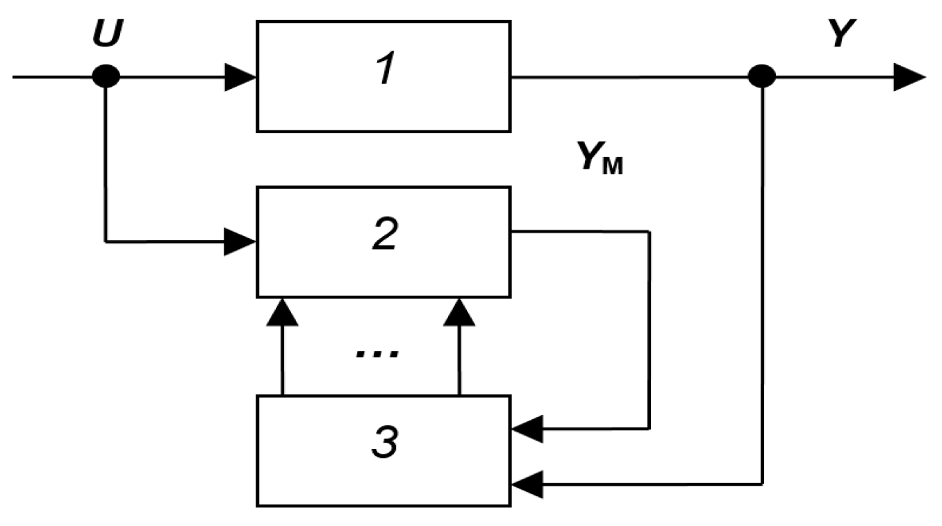
Figure A44.
SAS from [28]: 1—object, 2—controller, 3—object model, 4—model tuning unit, 5—computing device, 6—executive body, 7—identification unit, 8—self-tuning unit.
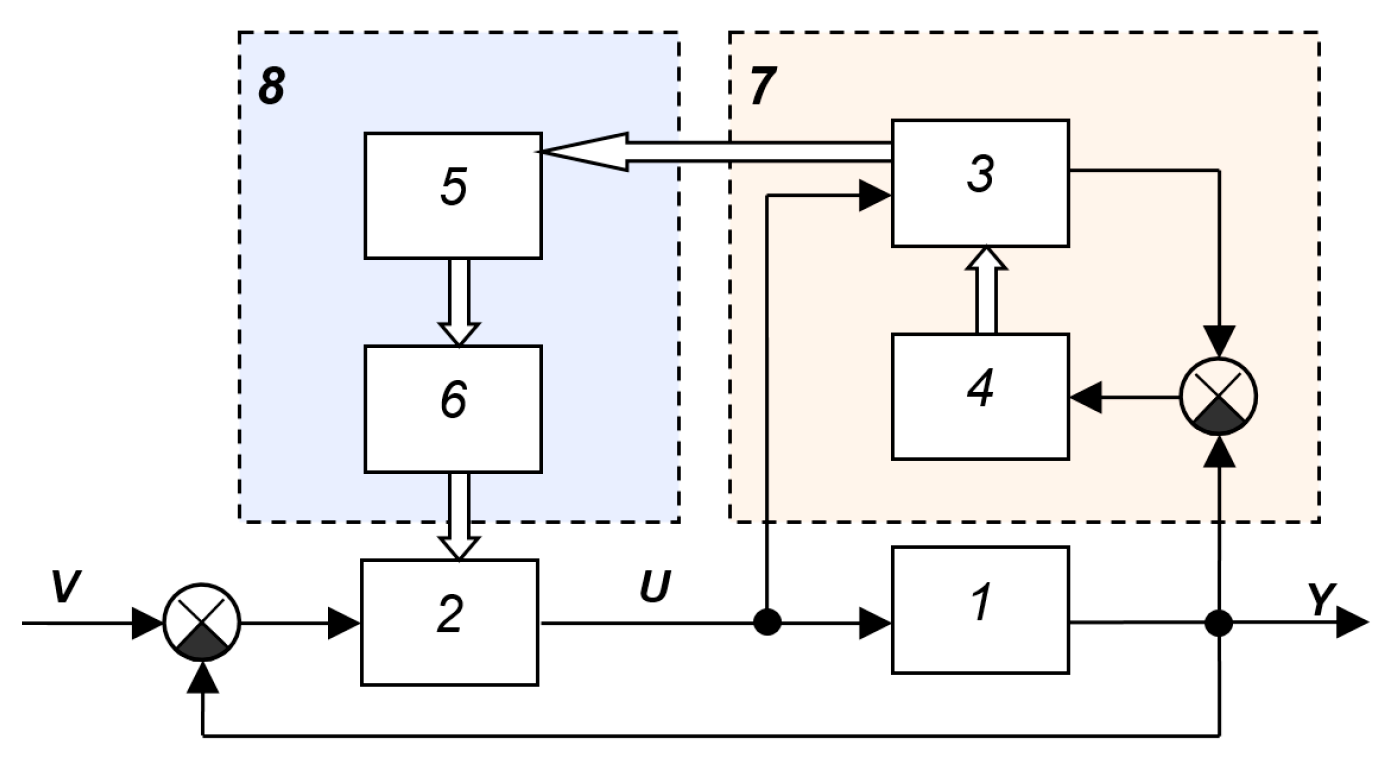
Figure A45.
SAS from [28]: 1—control object with extreme characteristics, 2—regulator, 3—model, 4—filter, 5—converter, 6—tuning block (models), 7—program block (tuning calculation device).
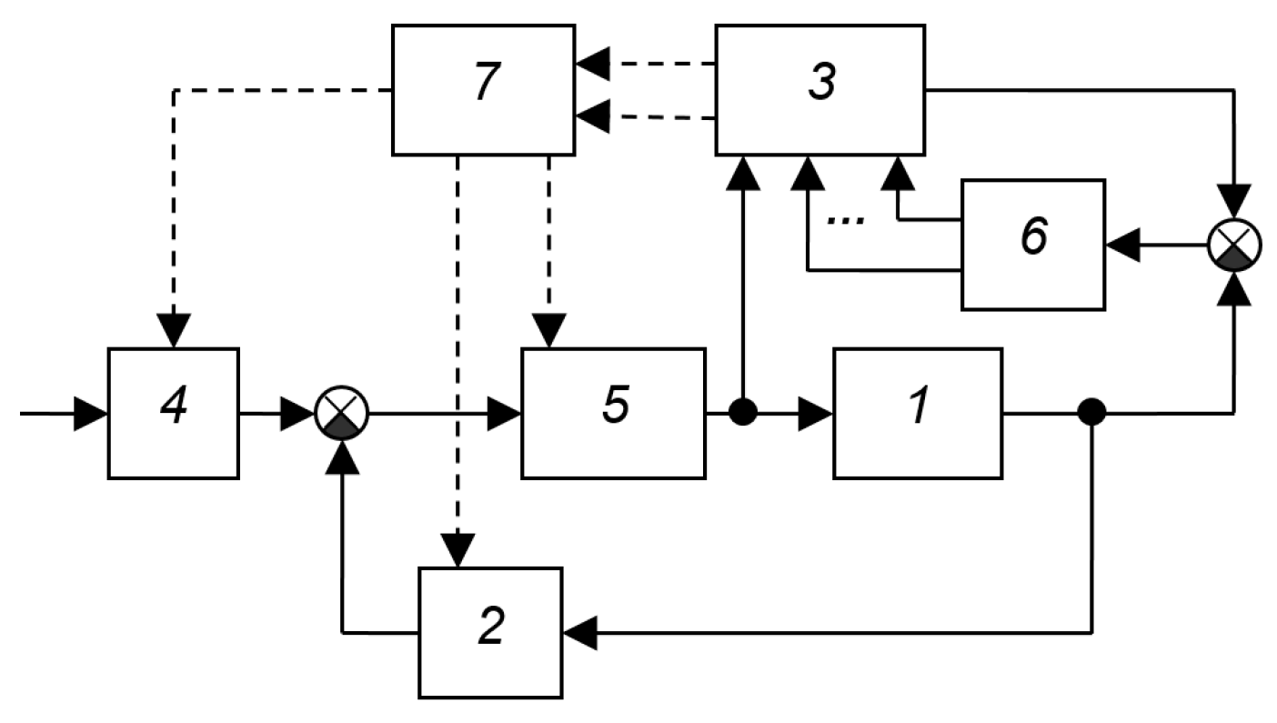
The circuit shown in Figure A46 [29] is distinguished by its connection to the input signal, as has already been noted: for servo systems, such a connection is insignificant, and if it is significant for a given system, it should be classified as a system with adaptation based on the input signal. This structure also includes a connection to the object. This indicates the use of the assumption that the object can be influenced not only through its input signal, but also in some other way. Such an approach is unjustified. All possible types of influence on the object should be reduced to the form of control signals, and all of them are generated by the controller. If, to control a single output variable, it is possible to influence an object not through one control channel, but through several, this should be taken into account in the structure of the circuit, i.e., in the main control loop. Control methods with an excessive number of inputs are discussed in various literature, including [41].
The above remark is also true for the SAS shown in Figure A47 from [36]. It shows an exotic structure of an object that consiSAS of three series-connected aperiodic links, and it is possible to apply a control action to the last link. If no amplitude restrictions are imposed on the input signals applied to the adder in the object before the element with the transfer function W3, then the actions on the second input seem inappropriate. Indeed, if they are set equal to zero, U = 0, we obtain an object consisting only of the transfer function W3. And since the first two transfer functions of the object introduce their own inertia, the possibility of excluding them from the circuit allows us to increase the object’s performance.
In the device shown in Figure A48 from [29], the dynamic characteristics are determined by the correlation of the output signal of the object with the delayed signals. In this system, the multichannel multiplying and adding device 5 calculates the correlation between the delayed signals and the signal of the object; the analyzing device must determine the parameters of the object from these correlation values. In this structure, naturally, the parameters of the complete circuit consisting of the regulator 2 and the object 1 are determined, but since the regulator is known, calculating the dynamic model of the object will not be difficult if the dynamic model of the complete circuit, including the regulator and the object, is known.
Figure A46.
SAS from [29]: 1—object, 2—controller, 3—process evaluation device, 4—external signal evaluation device, 5—logical element, 6—actuator.
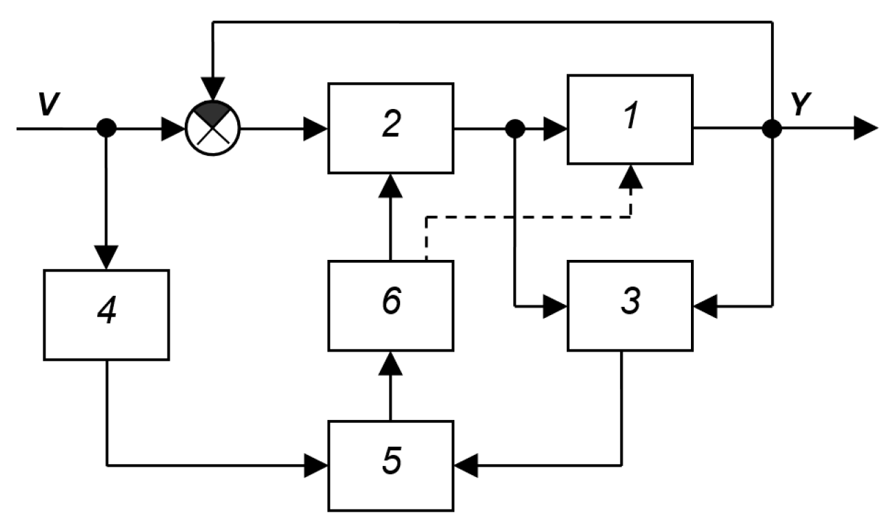
Figure A47.
SAS from [36]: 1—object, 2—regulator, 3—correcting and computing device, 4—signal analyzer, 5—internal signal analyzer, 6—calculator, 7—calculator.
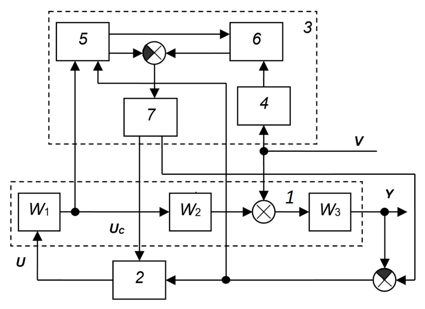
Figure A48.
SAS for the dynamic characteristics of an object [29]: 1—object, 2—controller, 3—white noise generator, 4—multi-channel time delay, 5—multi-channel multiplying and adding device, 6—characteristic analyzer, 7—self-tuning device, 8—correlator.
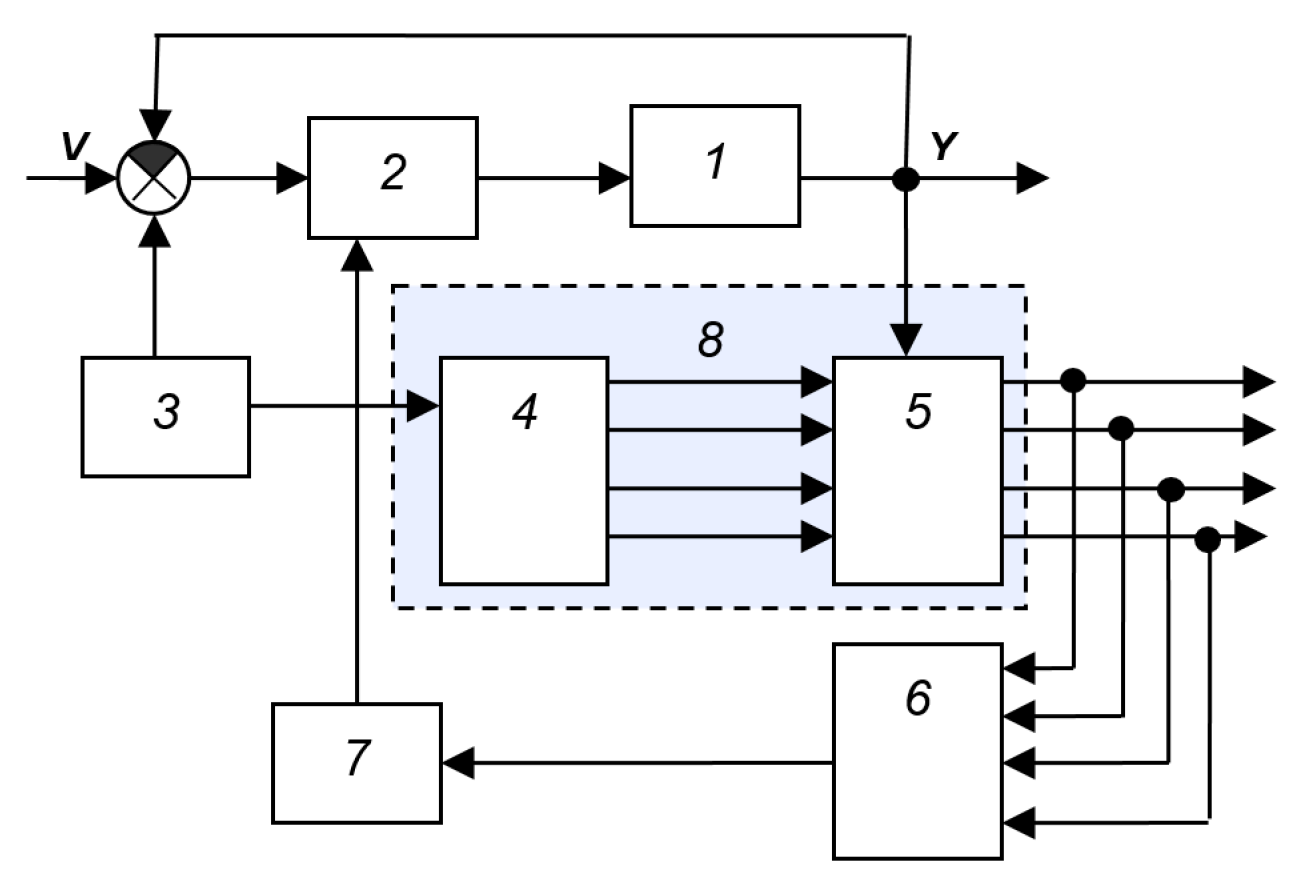
A disadvantage of this system is the need to introduce noise into the system, i.e., artificially degrade system performance to determine model parameters. Furthermore, the algorithm for determining model parameters from correlations is not entirely clear.
Figure A49 shows a variable-structure SAS with an adaptive control unit from [39]. “Spectrum analyzer” is inferior to the modern concept of “signal analyzer”, since in addition to decomposing the signal into a spectrum, phase relationships must also be taken into account. It is impossible to reconstruct a signal from a spectrum alone. These devices 5 and 6, in the modern interpretation, can be successfully replaced by devices such as wavelet converters, or by ADC blocks, as well as by a signal processor.
Figure A50 shows the SAS with a variable structure and an adaptive control device from [39]. At the current level of development of digital technology, it is not necessary to distinguish between a random access memory (RAM), a read-only memory (ROM), a computing or arithmetic logic unit (ALU), i.e., a microprocessor or a central processor, in functional diagrams, since any processor is considered to be equipped with the corresponding random access and read-only memory devices.
Figure A51 shows the block diagram of a rate-separated control system from [28]. This structure is essentially identical to the structure shown in Figure A50. Although the system operates in real time, the model is adjusted in accelerated time. In the device, the model is constructed based on a priori data and is continuously adjusted. The calculation of the optimal controller can be performed by simulation, in which various control options are calculated in accelerated time and the optimal option is selected.
Figure A49.
SAS with variable structure and adaptive control device from [39]: 1—control object, 2—part of the controller, optimal open-loop model, 3—part of the controller, inverse model of the object, 4—initial condition calculator, 5, 6—spectrum analyzer, 7—u(t) and y(t) calculator.
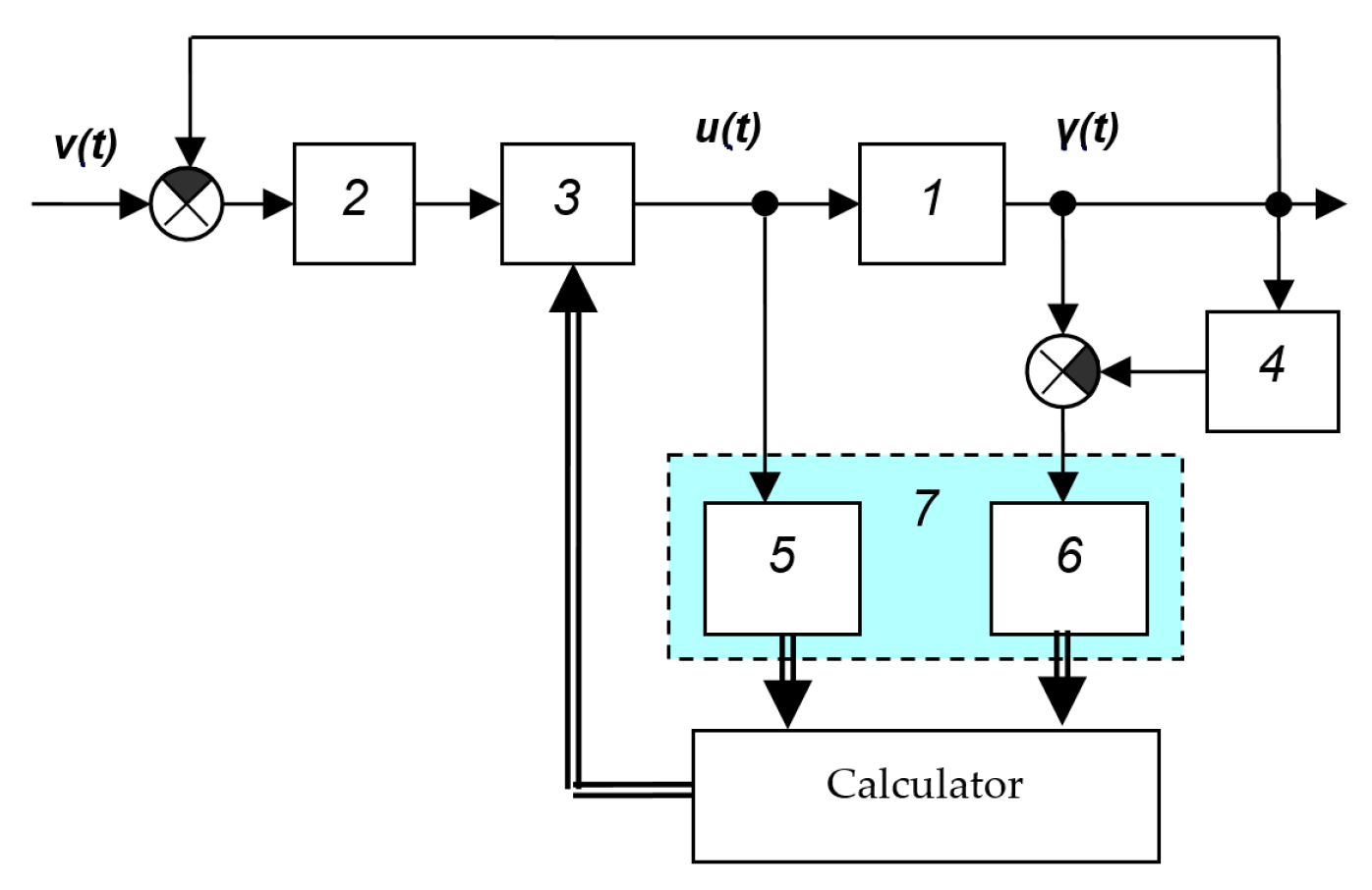
Figure A50.
SAS with variable structure and adaptive control device from the book [39]: 1—object, 2—control device, 3,4—computing device, 5—self-tuning device.
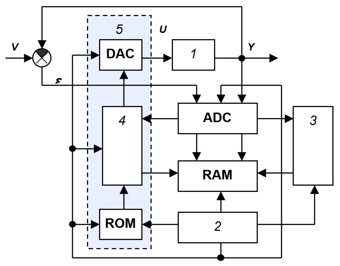
Figure A51.
SAS with tempo division from the book [28] (modeling—in accelerated time, control—in real time): 1—object, 2—fast model, 3—control device (regulator), 4—signal input device (ADC), 5—signal output device (DAC).
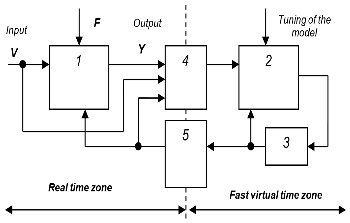
During the actual process, transient processes can be calculated with different models hundreds or thousands of times, depending on the difference between the actual time and the simulated time. Therefore, a controller is selected from a large set of analyzed options and then implemented in real time. This approach is extremely productive; more and more adaptive systems will be built on its basis in the future.
An example of a recent publication with a structure that identifies a control object model is the circuit shown in Figure A52 from the article [46]. This system proposes to separately identify the control object’s delay and the minimum-phase component of the object’s transfer function using two independent devices. The section proposing this structure does not contain clear algorithms for such separate identification, and the idea is not supported by specific examples that could be verified, for example, by numerical simulation.
Figure A52.
Structural diagram of the adaptive system with identification of the object model from [46].
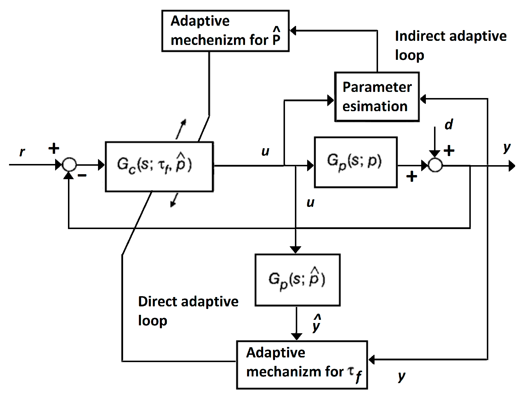
Systems with adaptation based on control error
This class can include systems in which the performance of the main loop is assessed based on the control error. An example of the simplest structure of such a system is shown in Figure A53 [29]. The operating principle of the system can be based on different approaches. For example, if the main loop, consisting of controller 2 and object 1, does not contain an integrator, the system in the absence of adaptive control device 3 will have a static error, but if adaptive device 3 includes an integrator, this static error will be eliminated. With this approach, the joint inclusion of controller 2 and adaptive device 3 can be transformed into an equivalent controller. The seemingly adaptive property of eliminating static error with respect to a static controller will become a common property of an astatic controller. The operating principle of the structure in Figure A54 can also contain a more complex algorithm. For example, the appearance in the error signal E, analyzed by device 3, of signs of approaching the stability boundary can serve as the basis for changing the controller parameters. Such a sign could be, for example, a sharp increase in the harmonic components of the error signal spectrum in a certain frequency range. As a result, device 3 can, for example, increase the gain of the differentiating path of controller 2 or decrease its overall gain. The system uses the error signal, ensuring its minimum by influencing the parameters or structure of the regulator, the object and the main feedback.
Figure A54 shows the SAS from [29], which is distinguished by a large number of elements and connections, namely: it allows the use of non-unit feedback and the impact not only on the regulator, but also on this element of non-unit feedback, as well as directly on the object.
Figure A53.
SAS with variable structure and adaptive control device from [29]: 1—object, 2—controller with variable structure, 3—adaptive control device.
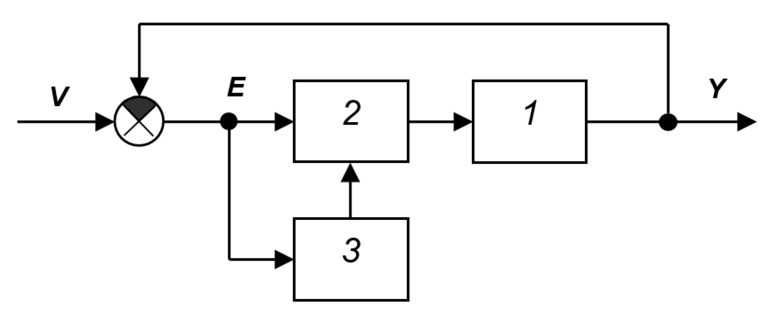
Figure A54.
SAS from [29]: 1—object, 2—controller, 3—self-tuning device, 4—main feedback.
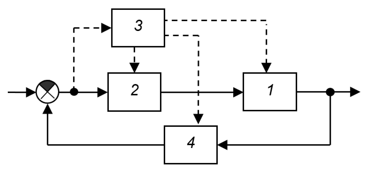
Non-unit feedback seems impractical, since it is more convenient to specify the prescribed output value in terms of the quantities that must appear at the output, but in a different signal form, i.e., solely in the form of electrical signals or digital codes. For example, if a system controls the laser frequency, it must employ a frequency increment detector that converts the signal into a voltage or code. Naturally, it is not the frequency itself that is fed to the subtractor element’s input, but its analog in voltage or code form. In other words, the feedback loop always includes an error signal sensor and a device that converts this signal into a usable, normalized signal representing the output increment relative to the prescribed value. However, for calculating the stability of locked-loop dynamic systems, representing this system element is not necessary. Therefore, it is not commonly depicted in block diagrams, although it is always implied. The feedback signal always undergoes transformation, in the sense of bringing the measured and prescribed values to a common scale. A change in this transformation can affect either the static coefficient or the dynamic characteristics. In the first case, this would mean changing the prescribed value, which is preferable to do by correspondingly changing the system’s input signal v(t), i.e., the task. In the second case, this means changing the dynamic properties of the main loop as a whole, which is more logically done by changing the parameters of the loop sequential controller. Thus, in general, with respect to the operating principle of feedback systems, the introduction of element 4 does not change the essence of the structure and is not fundamental. The introduction of the ability to directly influence the object, bypassing the controller, also classifies the system as exotic, since in the vast majority of cases, the object can only be influenced through its inputs, and in this case, changing the signal acting on the object is still the same influence on the structure or parameters of the controller, only depicted differently. Thus, the structure shown in Figure A55 apparently does not offer significant advantages over the structure shown in Figure A54.
Providing extreme tuning of closed-loop system qualities
This subclass includes systems that have a main control loop implemented based on traditional principles and have a loop for adjusting the controller parameters using extreme control methods to a state of extreme quality of the main loop.
Figure A55 shows the structural diagram reconstructed by us from the description in the text of the book [29]. The main circuit consists of object 1 and controller 2. The controller receives a feedback signal from logic element 5 and a test deviation signal from generator 7 via actuator 6. The actions of generator 7 lead to periodic changes in the signal in the main circuit. The proximity of the circuit state to the optimal setting is detected via the process evaluation device and the synchronous detector. The test action can also be fed as an additional signal arriving at the input of the object together with the control signal, as is done in the circuit shown in Figure A56, which is another version of the reconstruction of the same description in the text of the book [29]. A third version of the same reconstruction is shown in the circuit Figure A57 [29]. We did not find any specific structural diagrams in the literature that did not require reconstruction from the text.
Figure A55.
SAS from [29] (reconstruction from the text): 1—object, 2—controller, 3—process evaluation device, 4—synchronous detector, 5—logical element, 6—actuator, 7—generator, 8—self-tuning circuit.
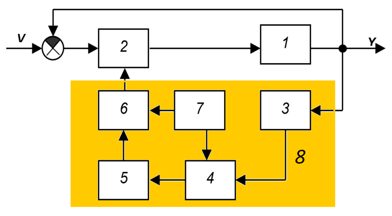
Figure A56.
SAS from the book [29] (reconstruction from the text): 1—object, 2—controller, 4—process evaluation device, 5—synchronous detector, 6—logical element, 7—actuator, 8—generator, 9—self-tuning circuit.
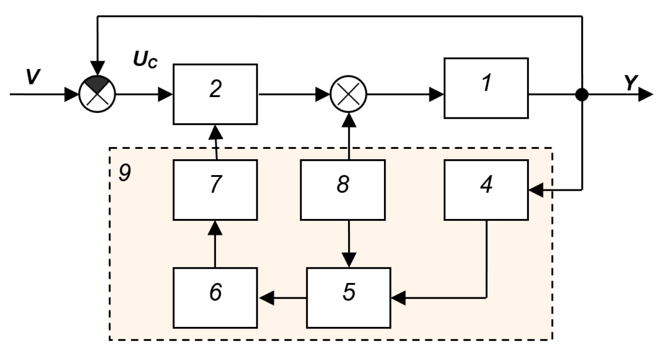
Figure A57.
SAS from the book [29] (reconstruction from the text): 1—object, 2—controller, 4—process evaluation device, 5—external signal evaluation device, 6—logic element, 7—actuator.
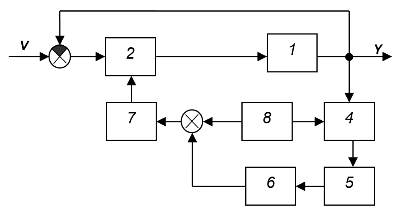
On the equivalent transformation
Let us consider SAS by Figure A2 is given as an example. It is assumed that the system has not only a main control loop formed by elements with transfer functions W1, W2, and W4, but also an additional loop formed by elements with transfer functions W3 and W4. The loop is locked by a subtractor, shown as a circle in which the inverting inputs are marked by a filled segment, and if the input segment is not filled, this means a non-inverting input. The main loop must ensure that the output value Y matches the specified value V. The additional loop, according to the developers, must ensure the desired dynamic qualities of this loop by correcting the output signal Y to its reference model YM.
This system is equivalent to the system shown in Figure A3, which is obtained using equivalent structural transformations. These structural transformations are based on equation transformation rules, which are symbolically represented in such structure diagrams. For example, based on the identity, an adder or subtractor element can be transferred from the input of a transfer function to its output, but the branch that was previously included in this adder element must acquire the same transfer function, as shown in Figure A58. Accordingly, transferring an adder from the output to the input requires adding to all incoming branches the transfer function inverse to that with respect to which the transfer is performed, as shown in Figure A59.
As can be seen from Figure A3, the resulting system consists of a closed loop of three elements, including the object, and an input structure that is a kind of filter. The properties of this input device do not contribute to noise suppression. They affect only the transformation of the reference signal . If a stabilization system is created, that is, for , these input elements do not affect the operation of the system and can be ignored. In this case, only a single feedback loop operates, including three series-connected elements with transfer functions, respectively, , , and . That is, the element with the transfer function simply does not work; it is not needed. This is also evident from the circuit in Figure A2 if we set
Figure A58.
Example of equivalent transformation of structural diagrams.
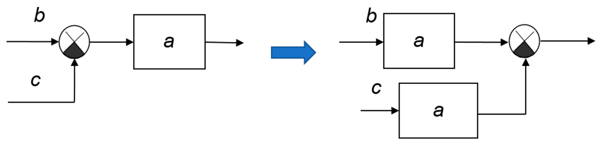
Figure A59.
Another example of equivalent transformation of structural diagrams: b—the first signal; c—the second signal, a—transfer function or gain of the element, 1/a—inverse transfer function of inverse gain.
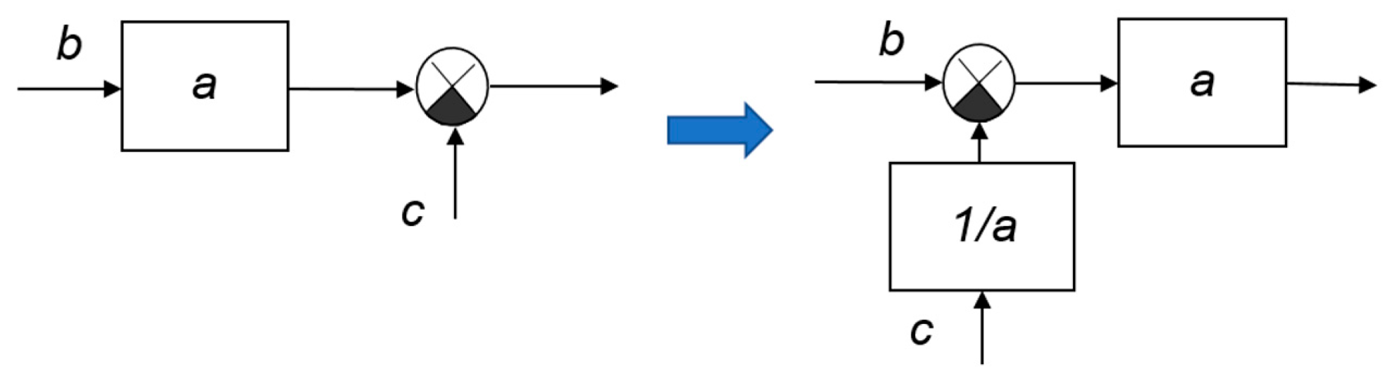
Any control system requires solving two problems: first, the output value must correspond as closely as possible to the input value; second, this correspondence must be maintained even under the influence of processes that transform the mathematical model of the object into a non-stationary one. These processes in this case are referred to as a generalized disturbance F(t), which affects not the output signal, but the mathematical model of the object.
If the reference signal is not strictly zero but remains constant over time, then even in this case, only the loop consisting of elements W1, W2, and W4 is actually functioning in the system. Consequently, the structure shown in Figure 2 (in the main part of the paper) cannot be considered an effective adaptive system. The adaptive loop in it is ineffective when the reference signal is zero or constant. If changes in the mathematical model of the object disrupt the stability of the loop consisting of these three elements, the system will lose stability, meaning its adaptive properties will not be ensured.
But if the given circuit consisting of elements W1, W2, and W4 is sufficiently efficient in itself, then it reduces the control error E to zero. In this case, both problems are solved: the system’s output signal V will replicate the signal arriving at the input from the filter output formed at the input by three elements with transfer functions W3, W4, and , and the influence of the disturbance F will be minimized. This loop will operate equally efficiently regardless of the value of , even in the case of .
For this reason, we prefer the control structure that remains if we remove the filter at the input of the system shown in Figure A2 and combine the elements with transfer functions W2 and W4 into a single structure called a “sequential controller.”
Therefore, the block diagram shown in Figure A25 is basic; it reflects all possible types of successfully operating connections and there are no connections that could not work. Indeed, there is a basic circuit consisting of elements: object 1, controller 2, and device 3, which provides adaptive properties. This device receives the system’s input signal , called the reference, the controller’s output signal , which is also the object’s input signal, and the object’s output signal , which is also the output signal of the entire system. In this structure, device 3 does not receive an error signal , but it can easily be calculated since the error is equal to the difference between the reference and the object’s output signal, and both of these signals are fed to the inputs of device 3. For this reason, device 3 does not need to be supplied with the task input but can be supplied with an error signal. Since the task, error, and output signal are related by a simple linear equation: .
Many publications devoted to adaptive control problems for objects with a non-stationary model discuss the problem itself quite clearly, but do not provide structures that could be used as prototypes for solving problems of interest to other authors working in the same field. A striking example of such an article is the publication [46].
As a result of the examples considered, the following classification of self-adjusting systems can be proposed.
1. Systems with adaptation to interference or other signals that indirectly or directly describe changes in the parameters of an object or the conditions of its operation.
2. Systems with adaptation to the input signal.
3. Systems with stabilization of the properties of the main circuit without object identification.
4. Systems with a reference, non-specifiable model of the object.
5. Systems with an object identifier or with a refined model of it.
7. Systems with adaptation based on control error.
8. Systems that ensure extreme quality of the main circuit.
Of greatest practical interest, due to their greatest versatility and best effect, are apparently systems with stabilization of the main circuit and systems with an identifier or with a refined model of the object.
We do not include in this classification systems with an object output prediction block (as with the Smith predictor), since this is a fundamentally different control principle; it is intended to reduce the delay effect, and not to solve the problem of changes in the mathematical model of the object.
References
- Lee, J.; Oh, K. An Adaptive PID Controller for Longitudinal Velocity and Yaw Rate Tracking of Autonomous Mobility Based on RLS with Multiple Constraints. Electronics 2025, 14, 4111. [Google Scholar] [CrossRef] [Scilit]
- Khoshbin, E.; Otis, M.J.D.; Meziane, R. Design an Adaptive PID Control Based on RLS with a Variable Forgetting Factor for a Reconfigurable Cable-Driven Parallel Mechanism. Robotics 2025, 14, 165. [Google Scholar] [CrossRef] [Scilit]
- Boubakir, A.; Souanef, T.; Labiod, S.; Whidborne, J.F. A Robust Adaptive PID-like Controller for Quadrotor Unmanned Aerial Vehicle Systems. Aerospace 2024, 11, 980. [Google Scholar] [CrossRef] [Scilit]
- Barrera- Fernández, J.M.; Hernández, J.P.M.; Escobedo, K.M.; Vázquez-Cervantes, A.; Solano-Vargas, J. An Adaptive PID Controller Utilizing a New Adaptive Exponent (Æ) Algorithm to Solve Derivative Term Issues. Algorithms 2025, 18, 391. [Google Scholar] [CrossRef] [Scilit]
- Yoo, M. Adaptive PID Control Based on Laplace Distribution for Multi-Environment Temperature Regulation in Smart Refrigeration Systems. Energies 2026, 19, 477. [Google Scholar] [CrossRef] [Scilit]
- Zhao, W.; Gu, L. Adaptive PID Controller for Active Suspension Using Radial Basis Function Neural Networks. Actuators 2023, 12, 437. [Google Scholar] [CrossRef] [Scilit]
- Arif, T.M.; Rahim, M.A. Agentic AI for Real-Time Adaptive PID Control of a Servo Motor. Actuators 2025, 14, 459. [Google Scholar] [CrossRef] [Scilit]
- Qin, H.; Wang, L.; Wang, S.; Ruan, W.; Jiang, F. A Fuzzy Adaptive PID Coordination Control Strategy Based on Particle Swarm Optimization for Auxiliary Power Unit. Energies 2024, 17, 5311. [Google Scholar] [CrossRef] [Scilit]
- Almachi, J.C.; Vicente, R.; Bone, E.; Montenegro, J.; Cando, E.; Reina, S. Implementation of a Neural Network for Adaptive PID Tuning in a High-Temperature Thermal System. Energies 2025, 18, 3113. [Google Scholar] [CrossRef] [Scilit]
- Liu, C.; Liu, P.; Cheng, Y. Self-Coupling PID Control with Adaptive Transition Function for Enhanced Electronic Throttle Position Tracking. Symmetry 2025, 17, 673. [Google Scholar] [CrossRef] [Scilit]
- Ghamari, S.M.; Habibi, D.; Aziz, A. Robust Adaptive Fractional-Order PID Controller Design for High-Power DC-DC Dual Active Bridge Converter Enhanced Using Multi-Agent Deep Deterministic Policy Gradient Algorithm for Electric Vehicles. Energies 2025, 18, 3046. [Google Scholar] [CrossRef] [Scilit]
- Noordin, A.; Mohd Basri, M.A.; Mohamed, Z. Adaptive PID Control via Sliding Mode for Position Tracking of Quadrotor MAV: Simulation and Real-Time Experiment Evaluation. Aerospace 2023, 10, 512. [Google Scholar] [CrossRef] [Scilit]
- Ding, Z.; Yao, Y.; Gao, S.; Yang, X.; Li, C.; Ren, J.; Dong, J.; Wu, J.; Ma, F.; Liu, X. Research on Variable Universe Fuzzy Adaptive PID Control System for Solar Panel Sun-Tracking. Sustainability 2026, 18, 1503. [Google Scholar] [CrossRef] [Scilit]
- Liu, D.; Zhao, S.; Zhang, J. Adaptive PID Control of Hydropower Units Based on Particle Swarm Optimization and Fuzzy Inference. Water 2025, 17, 1512. [Google Scholar] [CrossRef] [Scilit]
- Ding, Y.; Ren, X.; Zhang, X.; Liu, X.; Wang, X. Multi-Phase Focused PID Adaptive Tuning with Reinforcement Learning. Electronics 2023, 12, 3925. [Google Scholar] [CrossRef] [Scilit]
- Kroičs, K.; Būmanis, A. BLDC Motor Speed Control with Digital Adaptive PID-Fuzzy Controller and Reduced Harmonic Content. Energies 2024, 17, 1311. [Google Scholar] [CrossRef] [Scilit]
- Gao, Y.; Zhu, W. A Segmented Adaptive PID Temperature Control Method Suitable for Industrial Dispensing System. Electronics 2025, 14, 2306. [Google Scholar] [CrossRef] [Scilit]
- Liu, J.; Fang, H.; Xu, J. Online Adaptive PID Control for a Multi-Joint Lower Extremity Exoskeleton System Using Improved Particle Swarm Optimization. Machines 2022, 10, 21. [Google Scholar] [CrossRef] [Scilit]
- Zeng, X.; Wang, W.; Wang, H. Adaptive PI and RBFNN PID Current Decoupling Controller for Permanent Magnet Synchronous Motor Drives: Hardware-Validated Results. Energies 2022, 15, 6353. [Google Scholar] [CrossRef] [Scilit]
- VisSim Official Web. Available online: https://www.vissim.no/ (accessed on 6 February 2026).
- Asset, A.; Zhmud, V.; Mansurova, M.; Sarsenbayev, N.; Bayandina, G.; Kuandikova, G. Analysis of alternative controller structures for modeling and controlling a multi-channel water plant. In Proceedings of the 2025 IEEE 5th International Conference on Smart Information Systems and Technologies (SIST), Astana, Kazakhstan, 14–16 May 2025. [Google Scholar] [CrossRef] [Scilit]
- Zhmud, V.; Dimitrov, L. Control of Linear Multichannel Objects with Numerical Optimization. Appl. Sci. 2025, 15, 8927. [Google Scholar] [CrossRef] [Scilit]
- Zhmud, V. Controlling of Multichannel Objects with Non-Square Transfer Function. Automation 2025, 6, 27. [Google Scholar] [CrossRef] [Scilit]
- Zhmud, V.A. Increasing Dynamic Control Accuracy by Increasing the Order of Integration. Advances in Transdisciplinary Engineering. In Applied Mathematics, Modeling and Computer Simulation; IOS Press Book: Amsterdam, The Netherlands, 2024; Volume 61, pp. 597–605. [Google Scholar] [CrossRef] [Scilit]
- Zhmud, V.; Dimitrov, L. Using the Fractional Differential Equation for the Control of Objects with Delay. Symmetry 2022, 14, 635. [Google Scholar] [CrossRef] [Scilit]
- Asset, A.; Mansurova, M.; Zhmud, V.; Kopesbaeva, A.; Dzheksenbaev, N. Investigation of linear models for control of water flow and temperature in a water supply system. Indones. J. Electr. Eng. Comput. Sci. 2024, 35, 113. [Google Scholar] [CrossRef] [Scilit]
- Zhmud, V. Numerical Optimized Control of Object with Hysteresis with Smoothing Deviation. In Applied Mathematics, Modeling and Computer Simulation: Proceedings of the 3rd International Conference (AMMCS 2023); SAGE Publications Pvt. Ltd.: London, UK, 2023; Volume 42, pp. 920–927. [Google Scholar]
- Aleksandrovsky, N.M.; Egorov, S.V.; Kuzin, R.E. Adaptive Systems of Automatic Control of Complex Technological Objects; Aleksandrovsky, N.M., Ed.; Energia Publishing House: Moscow, Russia, 1973. (In Russian) [Google Scholar]
- Kuropatkin, P.V. Automatic Control Theory: A Textbook for Electrical Engineering Majors at Universities; Vysshaya Shkola Publishing House: Moscow, Russia, 1973. (In Russian) [Google Scholar]
- Voronov, A.A.; Kim, D.P.; Lokhin, V.M.; Babakov, N.A.; Voronova, A.A.; Diduk, G.A.; Dmitrieva, N.D.; Mensky, B.M.; Popovich, P.N. Automatic Control Theory: A Textbook for Universities in the Specialty “Automation and Telemechanics”: In 2 Parts, 2nd ed.; Voronov, A.A., Ed.; Part II. Theory of Nonlinear and Special Automatic Control Systems; Vysshaya Shkola Publishing House: Moscow, Russia, 1986. (In Russian) [Google Scholar]
- Pupkov, K.A.; Egupov, N.D. (Eds.) Methods of Classical and Modern Automatic Control Theory: A Textbook in 5 Volumes; Volume 5. Methods of Modern Automatic Control Theory; Publishing House of N. E. Bauman Moscow State Technical University: Moscow, Russia, 2004. (In Russian) [Google Scholar]
- Athans, M.; Falb, P. Optimal Control; Mashinostroenie: Moscow, Russia, 1968. (In Russian) [Google Scholar]
- Chaki, F. Modern Control Theory. Nonlinear, Optimal, and Adaptive Systems/Translated from English; Raibman, N.S., Ed.; Mir: Moscow, Russia, 1975. (In Russian) [Google Scholar]
- Kos, T.; Huba, M.; Vrančić, D. Parametric and Nonparametric PID Controller Tuning Method for Integrating Processes Based on Magnitude Optimum. Appl. Sci. 2020, 10, 6012. [Google Scholar] [CrossRef] [Scilit]
- Bistak, P.; Huba, M.; Vrancic, D.; Chamraz, S. IPDT Model-Based Ziegler–Nichols Tuning Generalized to Controllers with Higher-Order Derivatives. Sensors 2023, 23, 3787. [Google Scholar] [CrossRef] [Scilit] [PubMed]
- Vlasov, K.P. Theory of Automatic Control: A Textbook; Humanitarian Center: Kharkov, Ukraine, 2007. (In Russian) [Google Scholar]
- Kim, D.P. Automatic Control Theory. Multidimensional, Nonlinear, Optimal, and Adaptive Systems, 2nd ed.; Revised and Supplemented; FIZMATLIT Publishing House: Moscow, Russia, 2007; Volume 2. (In Russian) [Google Scholar]
- Solodovnikov, V.V. Statistical Dynamics of Linear Automatic Control Systems; Fizmatgiz Publishing House: Moscow, Russia, 1960. (In Russian) [Google Scholar]
- Antonov, V.N.; Prishvin, A.M.; Terekhov, V.A.; Yanchevsky, A.E. Adaptive Automatic Control Systems: A Tutorial; Yakovlev, V.B., Ed.; Leningrad University Publishing House: Leningrad, Russia, 1984. (In Russian) [Google Scholar]
- Chinaev, P.I. (Ed.) Self-Adjusting Systems; Naukova Dumka: Kiev, Ukraine, 1969. (In Russian) [Google Scholar]
- Bugrov, S.V.; Lisovoy, R.A.; Zhmud, V.A.; Kolker, A.B. Adaptive control system using the stabilizing effect of the controller coefficient deviation. Sci. Bull. Novosib. State Tech. Univ. 2010, 2, 157–160. (In Russian) [Google Scholar]
- Yakubov, O.E. (St. Petersburg Electrotechnical University “LETI”) Adaptive Electrohydraulic Servo Drive of an Aircraft. Available online: http://book.uraic.ru/files/spravka/105a.doc (accessed on 6 February 2026). (In Russian)
- Leva, A.; Magnani, G. Detecting Process Variations in Low-End PID Autotuners. In Proceedings of the 2002 IFAC, 15th Triennial World Congress, Barcelona, Spain, 21–26 July 2002. [Google Scholar]
- Ioannou, P.; Baldi, S. Robust Adaptive Control. In The Control Systems Handbook, Second Edition: Control System Advanced Methods; Levine, W.S., Ed.; CRC Press: Boca Raton, FL, USA, 2010; Volume 35. [Google Scholar] [CrossRef] [Scilit]
- Huang, H.-P.; Roan, M.-L.; Jeng, J.-C. On-Line Adaptive Tuning for PID Controllers. IEE Proc.-Control Theory Appl. 2002, 149, 60–67. [Google Scholar] [CrossRef] [Scilit]
- Wei, B. A Tutorial on Robust Control, Adaptive Control and Robust Adaptive Control—Application to Robotic Manipulators. Inventions 2019, 4, 49. [Google Scholar] [CrossRef] [Scilit]
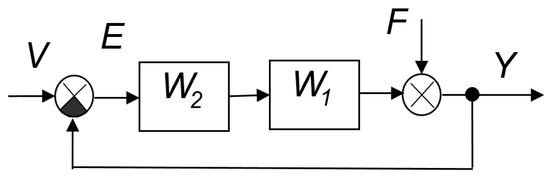
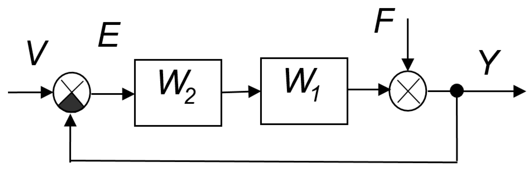
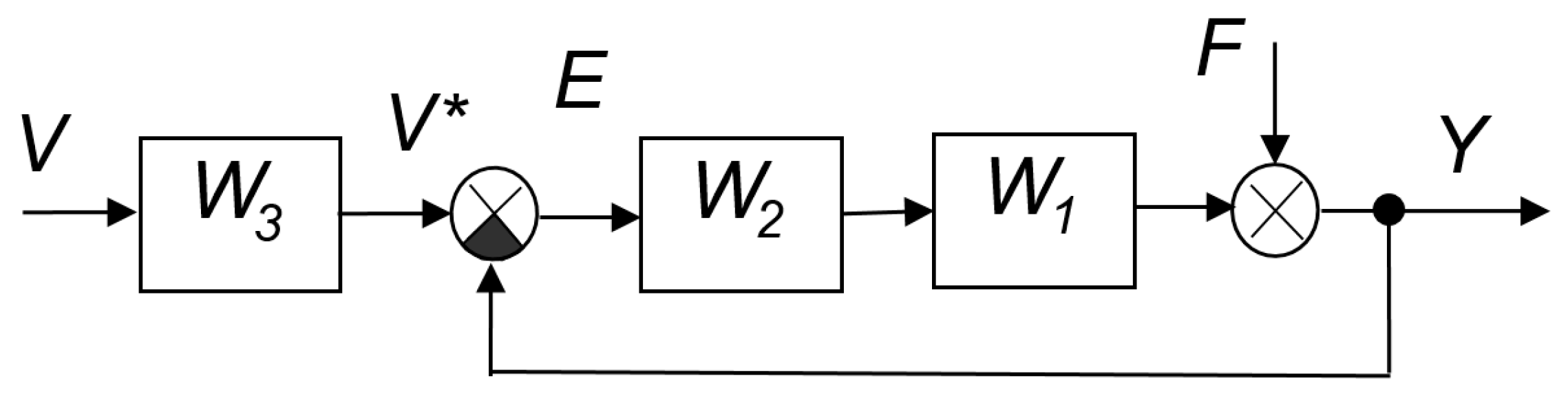
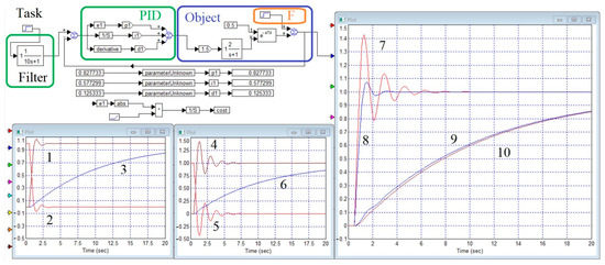
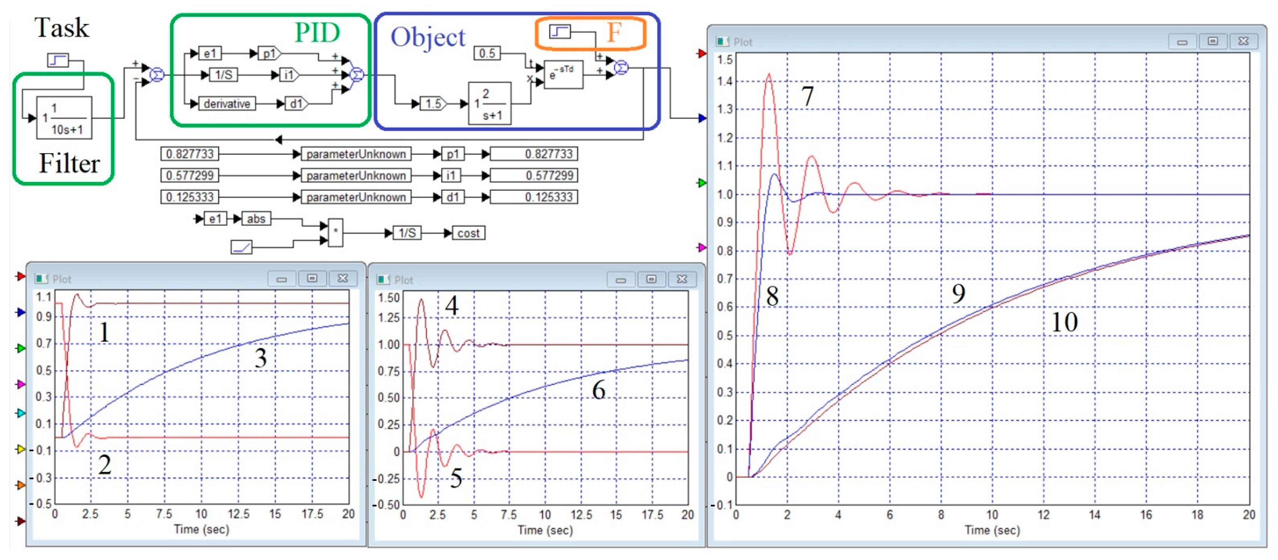
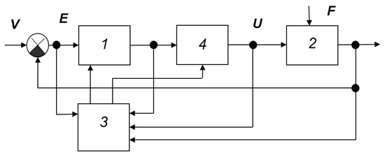
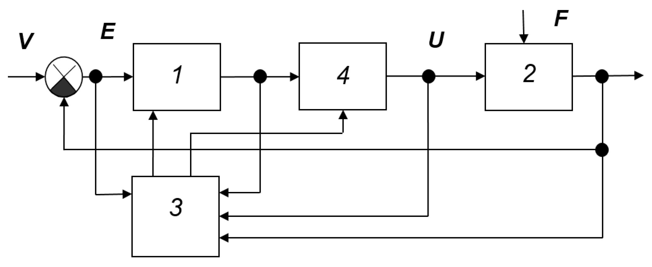
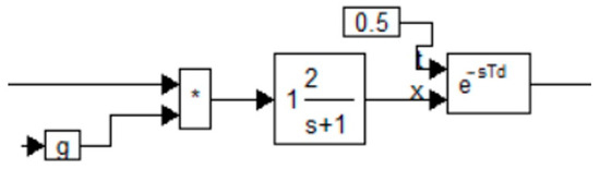
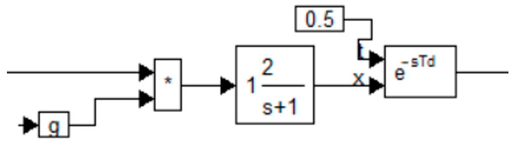
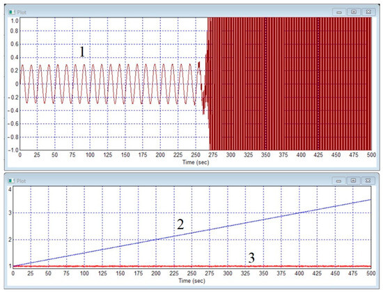
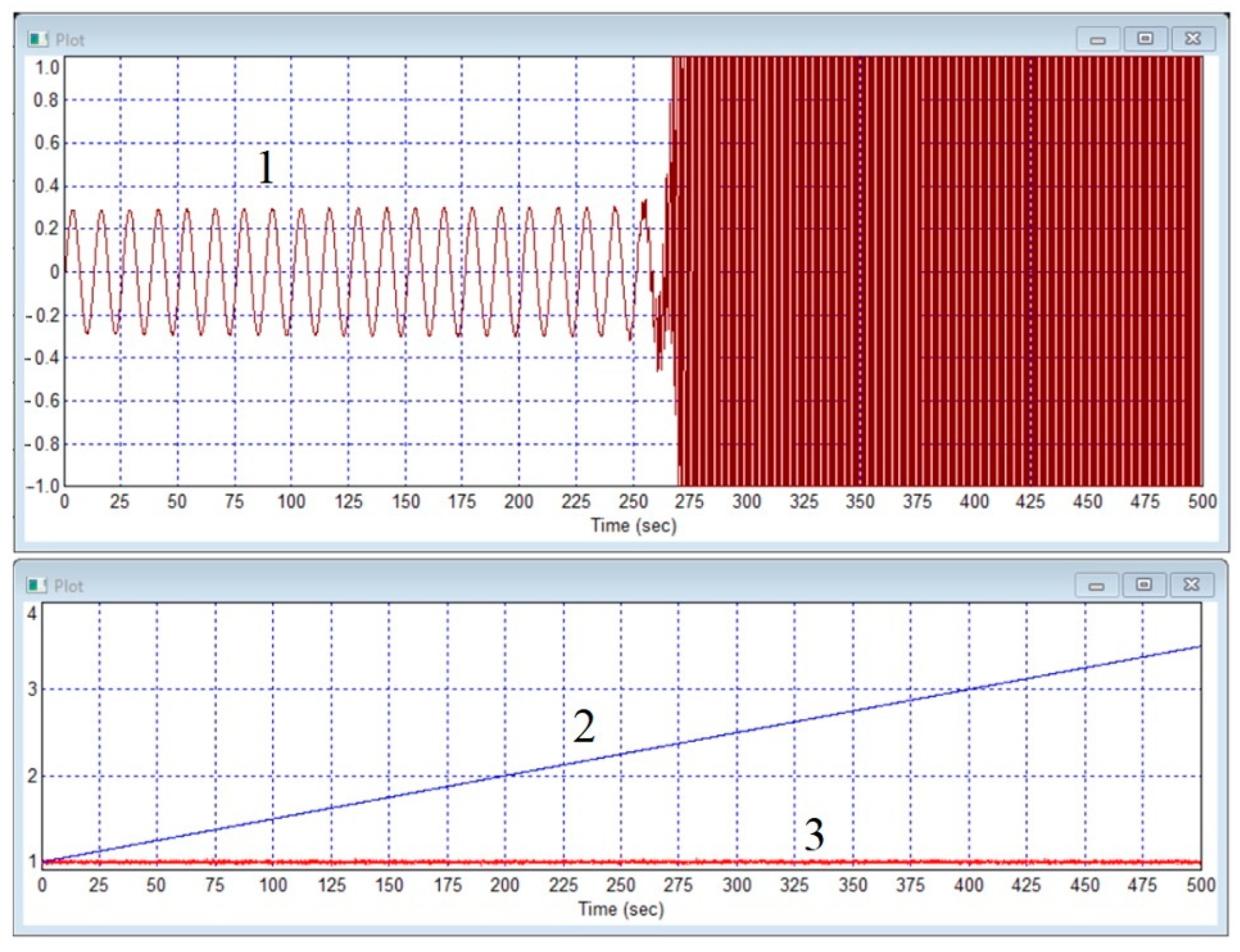
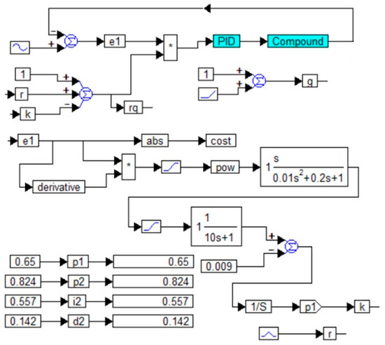
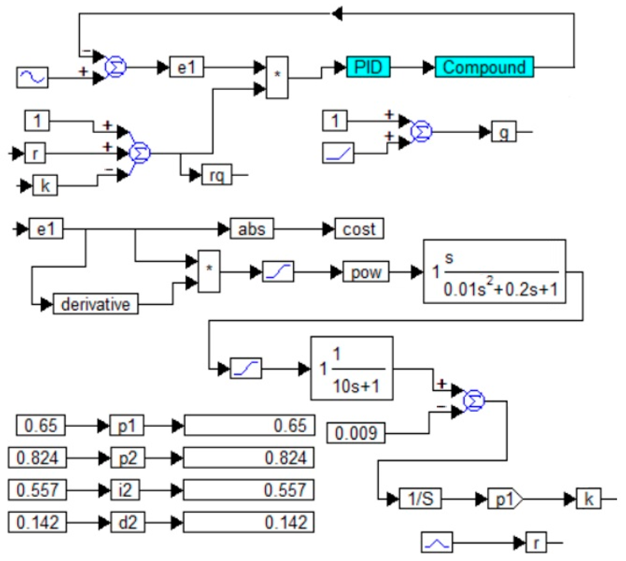
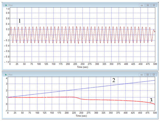
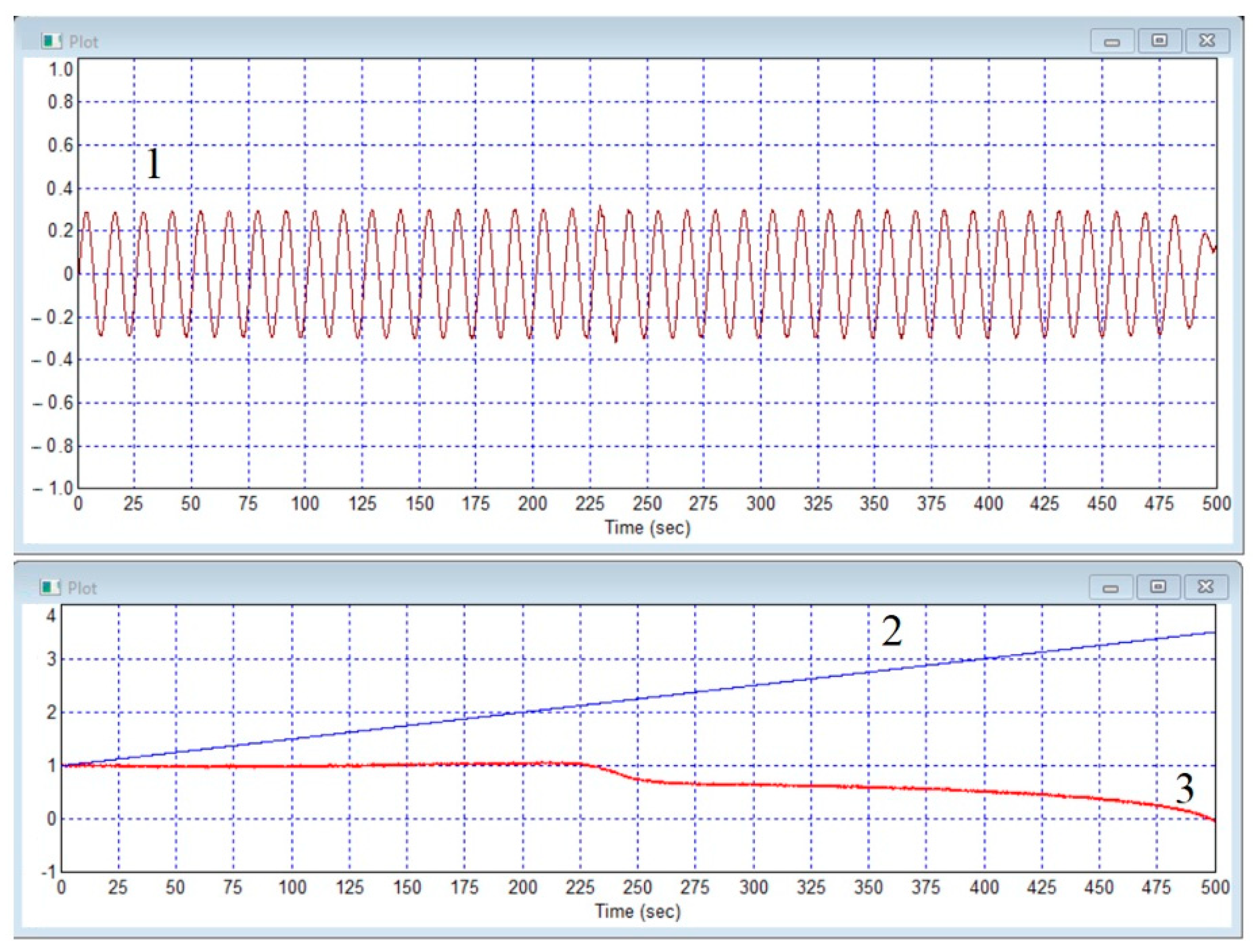
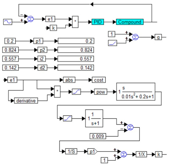
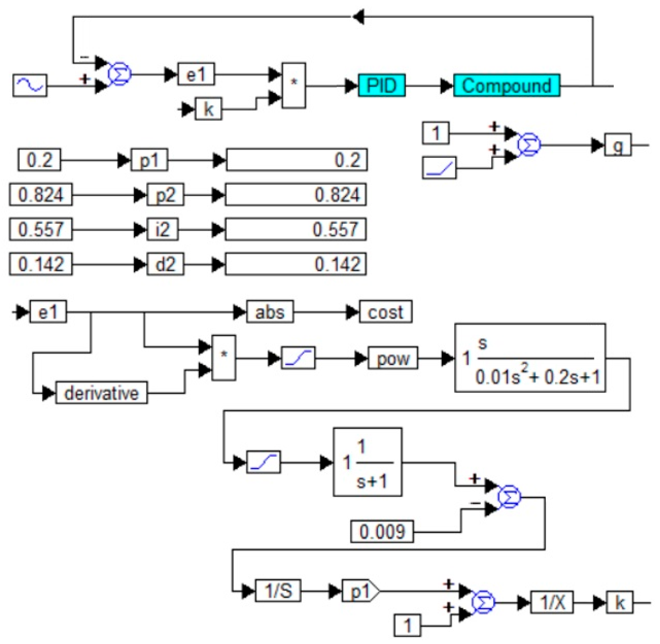
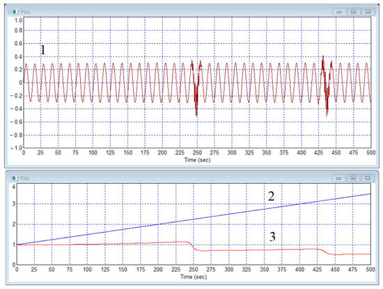
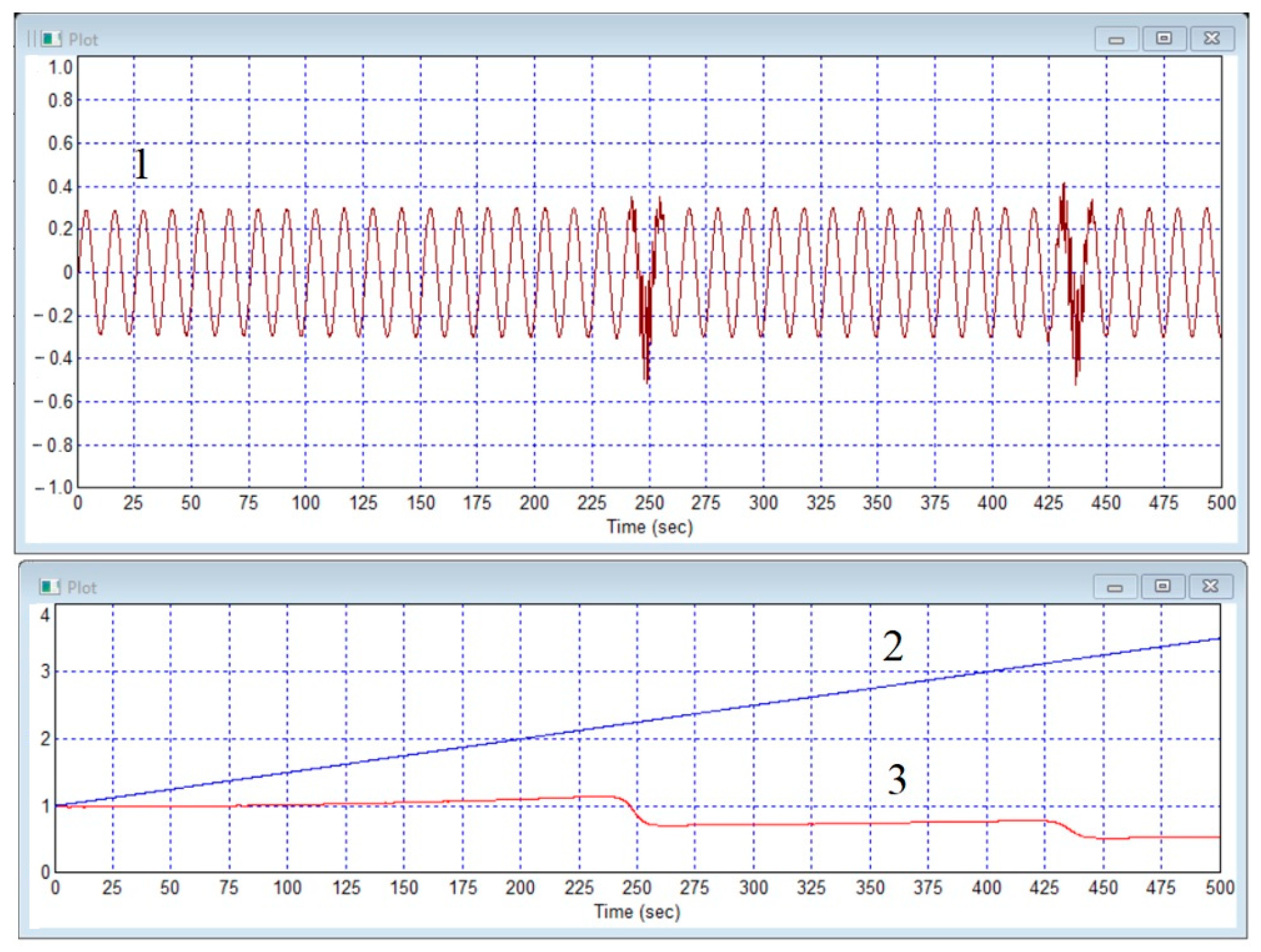
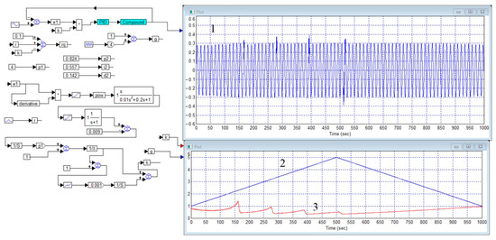
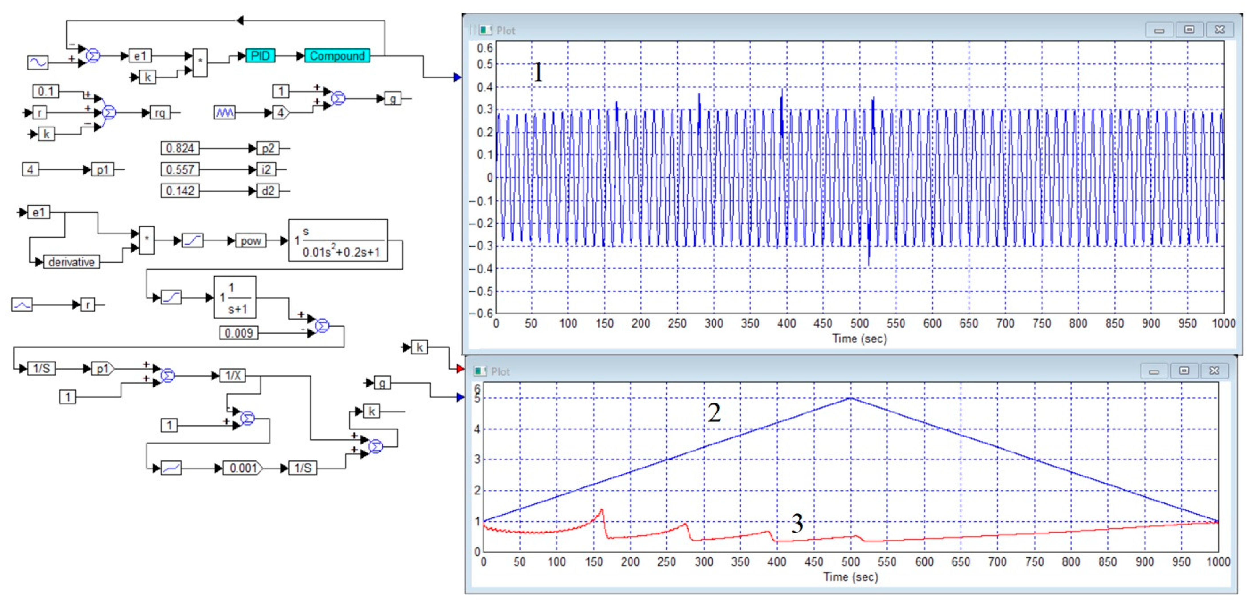
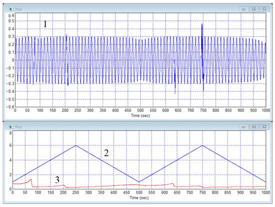
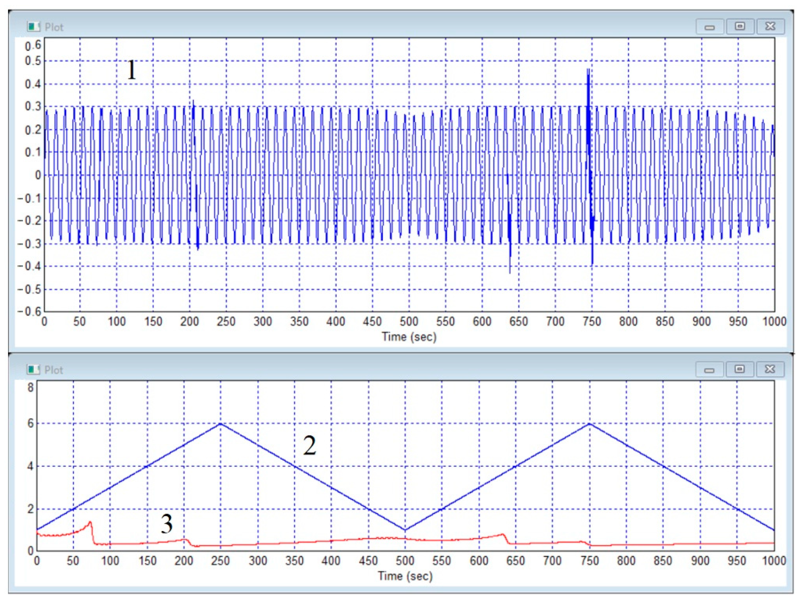
Disclaimer/Publisher’s Note: The statements, opinions and data contained in all publications are solely those of the individual author(s) and contributor(s) and not of MDPI and/or the editor(s). MDPI and/or the editor(s) disclaim responsibility for any injury to people or property resulting from any ideas, methods, instructions or products referred to in the content. |
© 2026 by the authors. Licensee MDPI, Basel, Switzerland. This article is an open access article distributed under the terms and conditions of the Creative Commons Attribution (CC BY) license.