


Abstract
This article proposes an integrated adaptive algorithm to control the accuracy and reliability of linear motion in electrohydraulic systems operating in dynamic modes and external loads. This algorithm has a multilevel parallel structure in which the physical model, extended measurement information, internal adaptive parameters, and the current of measurement and model uncertainties are combined and synchronized within a single loop. The proposed structure allows the real-time extraction of information about hard-to-determine dynamic characteristics of the electrohydraulic process, which is used to maintain consistency between the mathematical model and the actual behavior of the system, including in the case of rapidly changing modes and load variations. In addition, a functional observation layer for assessing the quality of measurement information is introduced, through which the sensitivity of adaptive mechanisms is managed, and the stability of the algorithm is maintained under degraded measurement conditions. Experimental results demonstrate a significant reduction in dynamic error and a sustainable improvement in the quality of tracking relative to a basic electrohydraulic system without algorithmic correction. This confirms the applicability of the proposed approach to real energy and industrial systems.
1. Introduction
Electrohydraulic systems are widely used in applications that require accurate positioning and motion control in the presence of external loads. This is primarily because of their high power density and ability to generate large forces with small structural dimensions [1,2,3,4,5,6]. Additional advantages are their ability to control movement smoothly and continuously over a wide range of speeds and loads, and their strong performance under harsh operating conditions, such as high loads, vibrations, and temperature changes [7,8,9]. Some prominent applications are found in machine tools and high-precision positioning systems [10,11,12], as well as in industrial robots and manipulators [13,14,15]. Electrohydraulic systems are also widely applied in automated production lines and test and loading benches [16,17,18,19,20]. Studies such as [10,11,12] demonstrate the suitability of electrohydraulic actuators for high-precision positioning tasks, while works [13,14] highlight their application in robotic and flexible systems. In addition, research in [16,17,18,19,20] focuses on their use in industrial processes and test environments, emphasizing the need for accurate and robust control under varying operating conditions.
In real operations, it is often necessary to perform complex trajectories in variable operating modes and in the presence of external forces, which place high demands on the accuracy and stability of the control system. Under these conditions, the limitations of electrohydraulic drives manifest themselves mainly in the form of dynamic errors, especially transients, changes of direction, and rapid deviations from the target. Studies such as [21,22,23] report that these errors are particularly pronounced during transient regimes and rapid changes in motion direction, while works [24,25,26,27] emphasize the influence of variable external loads and nonlinear system dynamics on positioning accuracy. These errors are caused by the combined action of nonlinear effects, hydraulic losses, compression of the working fluid, hysteresis in the control elements, elasticity of mechanical connections, the variable nature of the external load, and the dependence of dynamic parameters on the operating mode and the condition of the hydraulic environment [28,29,30,31]. As a result, the dynamics of the system often deviate from the behavior described by nominal or simplified mathematical models, which limits the ability of classical approaches to ensure high accuracy and stable operation in a wide range of dynamic modes [32,33].
Researchers have made numerous attempts to increase the accuracy of the dynamic positioning of electrohydraulic systems by improving algorithms for control and evaluation of states. Popular approaches include classical feedback and compensation schemes, as well as variants of state observers and Kalman filters, including linear and nonlinear extensions. The usual goal is to reduce the error between the set and achieved motion by more accurately estimating and compensating for dynamic deviations in transient modes and variable loads [34,35,36,37,38,39,40,41]. However, many of these approaches assume that the system model and noise characteristics of measurements are known perfectly or to a high accuracy, which limits their effectiveness under real-world conditions with variable dynamic parameters, external loads, and imperfect measurement information [42]. As a result, although these control methods have been successful in reducing systematic error, their robustness in highly dynamic modes is limited, motivating a broader approach that takes into account both model dynamics and the uncertainty of the measurement environment.
In complex dynamic systems, combining information from different measurement channels has proven to be an effective approach to improving dynamic positioning accuracy [43]. Various combinations of position, speed, pressure, and force sensors are used for this purpose; their data are combined through condition monitors or Kalman filters to extend the dynamic range and increase the reliability of estimates [44,45,46,47]. However, measurement channels are often treated as independent sources of information, and physical dependencies between them are only considered to a limited extent. The physical model is usually only involved in the prediction stage of the algorithm, which limits the possibilities for coordination between kinematic and dynamic quantities in highly dynamic modes of operation [48].
To overcome the limitations associated with the use of fixed model parameters, some researchers have used adaptive approaches to describe the dynamics of electrohydraulic systems, including online parameter assessment, adaptive condition observers, and identification methods [49,50,51]. These aim to compensate for nonlinear effects, hydraulic losses, and changes in external load, improving the correspondence between the mathematical model and the real process under changing operating conditions [50,52]. For instance, recent studies in adaptive control of electrohydraulic systems have emphasized the explicit compensation of nonlinearities such as friction and pressure–flow characteristics through dedicated control law design [53]. However, adaptive parameters are often interpreted as strictly physical quantities and determined separately from the main evaluation process [51]. The lack of a systematic mechanism for linking adaptation to the quality of measurement information and to the current dynamics of the system limits the possibilities for comprehensive and consistent compensation for model imperfections, especially in highly dynamic driving modes [52].
An important component of a state estimation algorithm is the method for selecting and tuning the covariance matrices of the model and measurement, since they determine how the measurement information is weighted and how the scattering of random error in the estimates of parameters from the state vector is managed [54]. In practice, the most common approach is to use fixed matrices and , determined on the basis of preliminary experimental estimates or empirical adjustment. Some authors have also proposed calculating these matrices adaptively by analyzing the statistical characteristics of residual deviations [55,56]. However, in existing works, covariance matrices are typically regarded as independent statistical parameters, with no direct connection to the physics of the system or to the real measurement environment, where correlations between measurement channels and the dynamics of parametric changes are often overlooked [57]. This limits the possibilities for adequately managing the confidence of measurements and balancing between sensitivity and robustness under highly variable operating conditions [54,56].
Management, monitoring, and adaptation algorithms have seen extensive development, but in much of the literature, the main focus has remained on minimizing the error between the set and evaluated values; the quality of the estimates has been analyzed primarily through accuracy indicators. In this approach, state estimation is often treated as a purely algorithmic task, with no systematic consideration of the consistency between the mathematical model, the measurement information, and the actual behavior of the system. This leaves metrological concerns—uncertainty, confidence in measurements, and stability of statistical characteristics—in the background. This is insufficient in highly dynamic modes, in which both model and measurement uncertainties change over time: the lack of a mechanism to monitor and manage the consistency of estimates can lead to good average behavior but with unstable statistical distributions and limited reliability in transients. Thus, there is a need to expand the classical evaluation structures by introducing targeted metrological control aimed at managing uncertainty and ensuring the sustainable behavior of algorithms under real operating conditions.
In this paper, an integrated algorithmic approach is proposed to achieve more accurate dynamic positioning of electrohydraulic systems by extending the structure of the Kalman filter. The approach uses advanced state estimation, combining information from real measurement channels and an additional pseudo-measurement channel based on the physical dependencies in the system, to achieve better consistency between the model and the real process.
A key feature of the algorithm is its adaptive internal coefficients, which act as a correction layer to compensate for the inevitable imperfections in the mathematical description of the electrohydraulic system. These coefficients are integrated directly into the framework for estimating states and allow the model to be adapted to changing conditions without requiring a strict physical interpretation of the parameters.
A metrological layer monitors the consistency between the evaluated states, the measurement information (including pseudo-measurement), and the mathematical model to manage the sensitivity of the adaptive mechanisms depending on the current quality of the estimates. Thus, the algorithm achieves targeted control over uncertainty by adaptively determining the covariance matrices of the model and measurement tied to both the dynamics of the adaptive parameters and the characteristics of the measurement environment.
2. Description of the Electrohydraulic System
A structural diagram of the electrohydraulic system is shown in Figure 1. The system includes an electromechanical module, a hydraulic actuator, measuring transducers, and a built-in processing and control computing unit. It is designed to realize precise linear movement along a predetermined trajectory, as is typically required for feeders in machine tools and positioning systems in automated production.
Figure 1.
Structural diagram of the electrohydraulic system: 1—hydraulic power unit; 2—electrohydraulic servo valve; 3—linear encoder; 4—attitude and heading reference system (AHRS) inertial measuring module; 5 and 6—pressure sensors; 7—hydraulic cylinder.
The electromechanical module consists of an asynchronous electric motor, a frequency inverter, and a hydraulic power supply unit with an integrated gear pump. The module includes an asynchronous electric motor ELPROM 5600 Troyan, Bulgaria with a rated power of 2.2 kW and a nominal rotational speed of 3000 min−1, controlled by a ELDI V-B, 2227 Bozhurishte, Bulgaria frequency inverter (3 HP/2.2 kW, output frequency range 0.5–400 Hz). The electric motor drives a M+S HYDRAULIC gear pump with a constant displacement of 4.5 cm3/rev, a nominal operating pressure of 200 bar, and a maximum rotational speed of 3500 rpm, which is integrated into the hydraulic power supply unit 1. The hydraulic power supply unit incorporates the oil reservoir and auxiliary hydraulic components and provides the required flow rate and pressure for the electro-hydraulic actuation subsystem.
The movement control is realized through an electrohydraulic servo valve (2), which regulates the supply of working fluid to the chambers of the hydraulic cylinder (7). The hydraulic cylinder is the actuator element of the system, and the linear movement of its output shaft realizes the set trajectory of the applied load.
Several measuring transducers located in the system monitor the movement and hydraulic processes. On the axis of movement of the cylinder is a linear-scale incremental encoder 3, Ditron DC10, resolution 0.005 mm, Chengdu, Sichuan, China. In addition, an attitude and heading reference system (AHRS) inertial measuring module 4, WT901SDCL-BT50, Hong Kong, China is used to record dynamic movement characteristics.
The hydrodynamic state of the system is monitored by two pressure sensors 5 and 6, COMECO PSPR–060–Q23 F-X, measuring range 0–250 bar, 6000 Stara Zagora, Bulgaria, located in the supply and return lines, respectively, of the hydraulic cylinder. These sensors provide information about the pressures in the operating chambers and the load on the actuator.
All measurement signals are received by a single-board computer Jetson Nano b01 16 GB eMMC 5.1, Santa Clara, CA, USA. The module provides synchronized data collection and processing, as well as generating the control signal for the servo valve, which closes the system’s control circuit.
3. Mathematical Model of the Electrohydraulic System and Structure of the Adaptive Kalman Filter
3.1. Mathematical Formulation of Dynamics and Measurement Model
The aim of this study is to develop a conceptual and mathematical model that ensures optimal accuracy in the execution of a given movement of the actuator of the electrohydraulic system. The assignment is determined by the displacement and speed of the linear shaft of the hydraulic cylinder, which describe the required trajectory, for example, when feeding into a machine tool or positioning in an automated system.
The model considers the vector of control variables as a function of the task, brought into the required form by a system of internal parameters characterizing the dynamics of the hydraulic and mechanical subsystems. Thus, the control signal is determined solely by the set displacement, speed, and acceleration. The Kalman filter is a self-adaptive mechanism that uses observations of the state to update the internal parameters of the model in real time to ensure accurate and metrologically consistent execution of the set motion.
The model includes dependencies that describe the linear motion of the actuator, force interactions, and pressure dynamics in the hydraulic cylinder, presented in vector–matrix form. This model serves as the core of the adaptive structure of the Kalman filter, in which a metrological layer provides monitoring and verification of the consistency between the evaluated and physically measured quantities. This layer is used to perform adaptive determination of the internal coefficients and covariance matrices of errors in the model and measurement, which improves the reliability and traceability of estimates under changing dynamic regimes.
On this basis, the state vector is formulated as follows:
where is the displacement of the actuator (the hydraulic cylinder output shaft), is the linear velocity of the output shaft, is its linear acceleration, is the external load applied to the output shaft, and is the difference in pressure between the two operating chambers of the cylinder.
The quantities in the vector characterize the main physical processes that determine the dynamics of the system and directly affect the accuracy of the movement of the actuator. The parameters , , and describe the kinematic dependencies of displacement, velocity, and acceleration, which determine the current state of the actuator and its response to changes in the governing signal. The magnitudes and represent the interactions between the hydraulic and mechanical subsystems: the load applied to the output shaft and the pressure of the working fluid that generates the controlling force, respectively. Including them in this form allows the model to take into account the real state of the system under different operating modes and provide a more accurate assessment of the parameters involved in the management process.
The vector of governing signals is defined as
where is the electrical signal to the servo valve, which determines the flow rate and direction of the working fluid. In the considered concept, a nominal control signal is introduced, defined as a function of the prescribed motion of the actuator. The assignment is described by the position , velocity , and acceleration , which are used to determine the control vector:
In its most general form, the relationship between the prescribed kinematic quantities and the nominal control signal can be represented by a linear combination:
where , , and are conversion coefficients by which the kinematic variables are brought into a scale suitable for hydraulic channel control. They are defined in advance at the system setup stage and determine the relationship between the command and execution subsystems, without describing the dynamic properties of the system itself.
In the real system, due to the presence of noise, nonlinearities, and hydraulic losses, the nominal signal does not ensure exact reproduction of the prescribed motion. Therefore, an adaptive Kalman filter structure is employed to estimate the system state and to ensure consistency between the model, the measurements, and the reference input.
As a result of this processing, the actual control signal is formed, which is applied to the servo valve and used in the dynamic model of the system.
For a clearer representation of the system structure and the relationships between its main components, a block diagram of the control system is presented in Figure 2. It illustrates how the reference signal, the measurements, and the control input are utilized within the adaptive Kalman filter structure to form a consistent estimate of the state vector. The obtained estimates are used to generate the actual control signal applied to the electrohydraulic system. At the same time, the control signal is also used in the filter model for state prediction at the next step, ensuring consistency between the mathematical description and the physical system. In this way, a closed-loop structure is realized, in which the interaction between the reference input, the model, and the measurements enables improved accuracy in reproducing the prescribed motion.
Figure 2.
Block diagram of the control of the electrohydraulic system with an adaptive Kalman filter structure.
The dynamics of the electrohydraulic system are described by a system of differential equations representing the relationships between the kinematic, force, and hydrodynamic quantities. The model accounts for the way in which the prescribed motion of the actuator is realized under the influence of the control signal , which has already been aligned with the current state of the system through the adaptive structure. These dependencies are formulated in the following system:
where , , , and are coefficients describing the dynamic interaction between load, speed, pressure, and acceleration, and , , and determine the hydrodynamic characteristics of the flow and pressure in the cylinder. The terms and are process noises that determine the uncertainty of the model and the unaccounted-for nonlinear influences.
In the system (5), the third equation implies that the acceleration is not considered as a dynamically evolving quantity; instead, it is determined by an algebraic condition derived from the balance of forces:
which ensures the relationship between the mechanical and hydraulic parameters of the system. This condition provides metrological consistency between the acceleration calculated by the model and the measured quantities and serves to form the pseudo-measurement in the measurement model.
The parameters , , , and represent physical parameters of the electrohydraulic system. The parameter denotes the effective piston area, is the equivalent mass of the moving parts, is the viscous friction coefficient, and is a coefficient characterizing the elastic and restoring forces in the system. These parameters are considered constant and are determined based on the structural characteristics of the system or through a preliminary identification procedure.
The inclusion of acceleration as a state variable allows the mechanical balance equation to be used as a pseudo-measurement in the measurement model. In this way, the estimation of the external load , which is not directly measured, is improved through the simultaneous use of the dynamic load model and the algebraic constraint of the force balance.
More specifically, the quantity is iteratively estimated within the Kalman filter as part of the extended state vector, with its value being formed through the combined effect of the prediction from the dynamic model and the correction imposed by the pseudo-measurement.
To facilitate further analysis and evaluation of dynamic errors, the system (5) is converted into a standard matrix form:
where is the state vector, and is the vector of process disturbances describing the uncertainties in the mechanical and hydrodynamic processes.
The elements of the matrices and are derived directly from the system (5), and each element is determined by the corresponding coefficient over the values of the state vector and the control variables in the equations for , , , , and . The following form is obtained:
This representation implies that the dynamics of displacement, velocity, and acceleration are described by a sequential relationship between kinematic quantities, while the change in the load force and the difference in pressures depend on the corresponding parameters , , , , , , and that reflect the characteristics of the mechanical and hydraulic subsystems.
Because it is difficult to define a theoretical model that simultaneously takes into account all the effects of nonlinearities, hydraulic losses, friction, and other internal interactions, which vary over the course of the system’s operation, the coefficients , , , and are included in the model. They are determined adaptively for each iteration of the Kalman filter algorithm, thus reflecting how their deviations from the nominal parameters change over time.
Each of these coefficients has a distinct physical meaning. First, characterizes the attenuation of forces and the changes caused by mechanical and hydrodynamic resistance. As can be seen from the fourth equation in the system (5), the parameter is related to the relationship between speed and load force, taking into account the energy exchange between motion and the pressure in the system. For its part, the coefficient determines the influence of the difference in pressures on the generated force, and describes the influence of acceleration and inertial effects on the overall dynamics.
By adaptively defining these four parameters, the model achieves a description close to the actual behavior of the mechanical part of the process and provides an opportunity for the dynamic compensation of nonlinear and time-varying factors. Section 3.3 discusses them in more detail and presents the methodology used to determine them.
To capture the full interaction between the mechanical and hydraulic subsystems, the model also includes a second group of coefficients, , , and , which describe the dynamics of the pressure difference between the two operating chambers of the cylinder. These parameters characterize the processes of attenuation and volumetric change, as well as the influence of the control signal on pressure, completing the description of the system. The coefficients are introduced in accordance with the fifth equation of the system (5), which represents the change in , and the methodology by which they are determined is discussed in Section 3.3.
The model employs two types of parameters denoted by : constant physical parameters , , , and , forming the base linear model, and adaptive coefficients , , , and , which are updated over time to compensate for nonlinear and time-varying effects. Additionally, the parameters , , and describe the pressure dynamics and are used as pre-identified constants.
In defining the measurement model, data from several independent sensor channels are used, which provide simultaneous observations of kinematic and hydrodynamic quantities. The actual measured parameters are the displacement , velocity , acceleration , and pressure difference .
The displacement is measured by an incremental linear encoder, which provides high accuracy in static and low-speed modes. Two independent measuring channels are used to determine the current speed values:
- -
- the incremental encoder, from which the speed is calculated as a derivative of the displacement, resulting in high accuracy but lower noise resistance to rapid changes
- -
- the inertial module, from which the speed provides good dynamic response at high speeds and accelerations but has a greater measurement variance
The acceleration is measured directly by the AHRS, which is mounted on the output shaft of the cylinder, and the difference in pressures is determined by two pressure sensors installed in the supply and return lines of the cylinder.
In addition to the real measurements, a pseudo-measurement based on the algebraic condition of (6), which expresses the balance of forces in the system, is also included in the model. This condition is considered as an additional “virtual” measurement channel that reconciles state assessments with the physical dependencies between them. For this purpose, a new measurement is defined:
the model of which is described by the expression
where the right-hand side represents the algebraic relationship between the acceleration and the other states of the system.
The inclusion of this pseudo-measurement improves the consistency between kinematic and hydrodynamic quantities, especially at high dynamic loads, by providing a metrologically correct connection between the physical model and the actual measurements.
Thus, the extended measurement vector takes the form
where the last element corresponds to the pseudo-measurement. The measurement model can be expressed in the following standard matrix form:
where is the measuring matrix, and is the vector of noise and error in measurement, with a covariance matrix .
The extended measuring matrix has the following form:
The last row represents the relationship between the acceleration and the other states defined by the algebraic condition (6).
The inclusion of the two independent speed channels ( and ) allows the filter to use the different noise characteristics of the sensors and adaptively determine the relative confidence of each channel through the covariance matrix .
To improve the signal-to-noise ratio of the rate calculated by the incremental encoder, a Savitzky–Golay filter is applied, which provides local polynomial smoothing of the data, without distorting the phase and dynamics of the measured signal [58,59,60]. This allows the instantaneous velocity to be determined reliably even in the presence of high-frequency noise and increases the accuracy of the combined assessment.
In this way, the two channels complement each other: the encoder provides high spatial resolution at low speeds, while the AHRS provides sensitivity to rapid changes, and their integration through the Kalman filter increases the stability and metrological consistency between the physical model and the actual measurements.
A structural diagram of the algorithm is presented in Figure 3. The model consists of five parallel operating and synchronized circuits in an iterative cycle. The first circuit is designed to determine the estimates of the state vector, and the second to calculate the covariance matrix of state errors . The third, fourth, and fifth circuits implement adaptive procedures to determine internal coefficients , , , and , to update the covariance matrix of measurement errors and noise, and to adaptively determine the variances of error and noise in the model, respectively. Each of these three circuits includes a starting block with preliminary values and a generalized adaptation block, the internal dependencies of which will be discussed in detail in the following subsections.
Figure 3.
Modular flowchart of the generalized algorithm of the Kalman filter and its adaptive components.
After the final assessment of the states, a metrological layer monitors the consistency between the evaluated and measured quantities and feeds information to the adaptive blocks to correct the internal coefficients and covariance matrices of the model and measurement. The individual functional blocks are organized in a structured manner within a single iterative cycle, which ensures efficient execution of the algorithm without increasing computational time.
To clarify the functional organization of the model and the interrelations between its individual parts, Table 1 summarizes the main layers of the system, their roles in the adaptive algorithm, and the corresponding metrological functions.
Table 1.
Main layers of the adaptive model and their metrological functions.
The mathematical model of the electrohydraulic system is formulated in continuous form as a system of differential equations, which allows a clear physical interpretation of the interactions within the system.
The algorithmic implementation of the model, including the Kalman filter and the adaptive procedures, is carried out in discrete time with a fixed sampling step .
In this context, the derivatives in the equations are approximated by finite differences, which allows the model to be directly used in an iterative form corresponding to the implementation of the algorithm. In this way, a separate discrete model is not derived; instead, the continuous formulation is used as the basis for numerical implementation in discrete time.
In addition, to evaluate the computational efficiency of the proposed algorithm, its implementation on the employed single-board computer (Jetson Nano B01, 16 GB eMMC) is considered. At the specified sampling step , the algorithm, including the Kalman filter, the adaptive procedures, and the metrological layer, is executed within each discrete cycle without accumulation of delay.
This ensures real-time operation and allows the application of the algorithm in closed-loop control of the electrohydraulic system. It should be noted that the parallel organization of the individual computational branches does not lead to a significant increase in computational time, which confirms the applicability of the proposed approach under dynamic regimes and industrial conditions.
3.2. Metrological Layer for Monitoring and Adaptive Model Verification
The metrological layer is a functional module in the adaptive model; its main role is to monitor the consistency between the measured and evaluated quantities, as well as to manage the process of updating the parameters and covariance matrices. In real time, it feeds corrective information to the adaptive procedures in order to maintain a balance between sensitivity and reliability.
The inputs to the metrological layer are the reference values of displacement and velocity, the values estimated by the Kalman filter, and the covariance matrix of the estimates . From these inputs, metrological consistency indicators, such as residual errors between measurements and forecast values, are calculated. These indicators are analyzed statistically and are used to adaptively determine confidence limits and variances, by which the current quality of the model is assessed. In the presence of inconsistency between the evaluated and set values, the metrological layer corrects the parameters affecting the adaptation: the internal coefficients and the elements of the covariance matrices and .
In this way, the metrological layer acts as a self-regulating accuracy mechanism that makes a dynamic correction to the adaptive calculations without disrupting the continuity of the iteration process. It provides the necessary connection between the physical model and the measurement system, controlling the metrological indicators to improve the reliability, traceability, and validity of the results. Thanks to its action, the adaptive model maintains the stability of estimates under variable operating modes, without reducing the speed of the algorithm and without compromising the consistency between the different circuits.
The mathematical description of the metrological layer is based on an estimate of the consistency between the given and estimated displacement and velocity values. For this purpose, in each iteration cycle, the momentary differences are determined:
These deviations are normalized by the current uncertainty of estimates derived from the covariance matrix of the states:
where and are the variances of the estimates and , respectively, derived from the covariance matrix .
Normalized residuals are combined into a summary metric of metrological consistency:
where and are weights determining the relative importance of the positional and velocity channels. Their values are calculated adaptively according to the variances of the respective estimates:
To provide an estimate of consistency over time, an average metric within a sliding window of steps is taken:
The variance of this indicator is also calculated:
The combination of these two quantities characterizes the current metrological consistency of the system because reflects the average level of coherence and its stability over time. On this basis, the metrological layer performs adaptive parameter management, attempting to maintain the indicator in a set eligibility interval and minimize the dispersion . The permissible thresholds are set at values and . When exceeds the upper limit, this indicates underestimation of noise or insufficient adaptation; as a result, the metrological layer increases the corresponding elements in the covariance matrices and and speeds up the process of updating the internal coefficients. At values below the lower threshold, overestimation of errors is assumed; in this case, the metrological layer reduces the corresponding variances and slows down the pace of adaptation in order to stabilize the estimates. The structural organization and sequence of operations in the metrological layer are presented in Figure 4.
Figure 4.
Structural block diagram of the metrological layer.
The combined assessment serves as the main criterion for the dynamic consistency of the model with the reference trajectory; the mechanism by which these adjustments are applied to the individual adaptive blocks is discussed in detail in the following subsections.
3.3. Adaptive Determination of Internal Coefficients
The internal coefficients , , , and characterize the dynamic interaction between load, speed, pressure, and acceleration in the electrohydraulic system. They are generalized parameters that compensate for imperfections in the mathematical description of the system resulting from nonlinearities, hydraulic losses, temperature influences, and changes in the characteristics of the fluid. Thus, these coefficients play the role of adaptive correction factors, through which metrological consistency is achieved between the model and the real process.
The dynamics of the load force on the output shaft of the hydraulic cylinder are determined by the fourth differential equation in the system (5). After discretizing with sampling interval and rearranging the terms, the equation can be rewritten as
where is the observed (or predicted by the Kalman filter) change in the load force, is the vector of the regressors containing the input variables, is the vector of unknown parameters, and is the residual error.
The vectors of the regressors and the unknown parameters are, respectively,
The “+” sign is used because all quantities related to the load exist only as posterior estimates corrected by the Kalman filter. The use of in the regressor vector ensures metrological consistency between the calculation of and the input data of the regression model. In (21), the vector of regressors includes all the factors that affect the change in force.
Since the load is not measured directly, the Kalman filter provides its assessment after the measurement correction in step . The change in load force in the interval is calculated from
This discrete derivative is an approximation of and is filtered by a Savitzky–Golay polynomial filter, which produces the quantity . This is used to suppress high-frequency noise components and to maintain the stability of parametric identification.
The algorithm determines the new parameter estimates at each iteration by minimizing the sum of the weighted squares of the errors. Initially, the following values are assigned:
where is the covariance matrix of the parameter estimates, and is a large initial uncertainty, which ensures quick adaptation in the first iterations for all .
Recursive dependencies are defined by
where expresses the difference between the observed and projected value of the change in external load,
Here, is the gain vector for the parametric update, which is determined by the expression
in which determines the extent to which new information affects the update of the estimated coefficients, and is the covariance matrix that describes the errors in determining the estimated coefficients in the step .
After each iteration, the covariance matrix is updated by
which reduces the uncertainty of the parameters in the accumulation of information and “forgets” older data in the case of . To ensure the physical validity of the evaluated coefficients, after each iteration, the parameters are limited to acceptable limits: , , , and the sign of is determined by the direction of acceleration.
The parameter is updated on each iteration according to the ratio between the actual and reference variance of the prediction error:
where is the reference (expected) variance of the error under normal stationary operation, which is calculated from
provided that the change in the error between successive steps does not exceed the threshold
On the basis of the resulting ratio the parameter is updated on each dependency iteration:
where is a coefficient determining the sensitivity of adaptation, is a coefficient that sets the margin of error deviation above which the adaptation reaches its maximum speed, and is the minimum allowable value of the parameter.
The reference variance serves as a stable benchmark against which the deviation of the current prediction error is evaluated. It is only updated when the system is in an established and metrologically consistent mode. This is checked using the indicators from the metrological layer: the average value and the dispersion . When they fall within preset permissible limits and , the reference variance is slowly updated with an exponential rule:
In the presence of instability or impaired coherence, the value of is kept unchanged to maintain a valid standard for comparison. When the current error variance increases above the reference (), the algorithm automatically reduces to speed up adaptation. In the stable mode (), the value of remains close to one, which ensures smooth and stable operation. In this way, the metrological layer regulates the permissible limits of dispersions and the sensitivity of the adaptive process, ensuring reliable coordination between the model and the real system. The structural diagram in Figure 5 illustrates the operation of the algorithm for adaptive determination of internal coefficients , , , and .
Figure 5.
Structural flowchart of the algorithm for adaptive determination of the internal coefficients , , , and .
The parameters , , and describing the dynamics of the hydraulic channel are determined in advance by an automated identification procedure, which is performed during the operation of the system in different modes. Because the hydraulic channel does not undergo rapid dynamic changes, these parameters are evaluated outside the Kalman filter structure and are subsequently used as constants in the pressure difference model defined by the fifth equation in the system (5). Once they have been determined, these parameters are used as physically based constants that describe the main mechanisms by which the hydraulic channel influences the pressure dynamics.
To calculate them, a regression is performed between the measured values of , the velocity , and the control signal , in which the derivative is evaluated from the current measurements of the system, after preliminary smoothing by a Savitzky–Golay filter. The parameters , , and are calculated using the recursive least-squares (RLS) method, providing a stable estimate in the presence of noise and dynamic loads. The resulting average values of the parameters are used as constants in the hydraulic channel model and are involved in the construction of the transition matrix and the matrix B of the control vector in the structure of the Kalman filter.
To ensure rapid convergence during the initial phase, large initial uncertainties of the parameter estimates are intentionally assigned. While this may lead to transient variations in the first iterations, their effect is inherently limited by the structure of the algorithm. In particular, the adaptive coefficient λ regulates the update rate, while the imposed parameter constraints and the metrological layer contribute to stabilizing the estimation process and suppressing high-frequency fluctuations. As a result, no significant oscillatory behavior affecting the actuator operation is observed.
3.4. Adaptive Determination of the Measurement Covariance Matrix
The covariance matrix of measurement is determined in accordance with the extended measurement vector presented in the model, which includes a displacement measurement, two independent speed estimates, a directly measured acceleration and pressure difference, and one pseudo-measurement. Because of the differences in dynamic sensitivity, the nature of the noises and the accompanying measurement errors in each of the channels, represented by the elements of the matrix , are updated with each iteration of the algorithm. This allows for the current operating conditions to be taken into account dynamically, including the occurrence of vibrations, nonlinearities, changes in load, and deterioration of the quality of measuring signals.
On the basis of the measurement vector defined in (11) and (12), the measurement error is defined in each discrete step as the difference between the measured quantities and the values predicted by the model:
where the measurement error vector has the form
In the following relations, the components of are marked with , as they serve as working residuals for the adaptation of the matrix .
The covariance matrix of measurement is defined in the standard way as the expectation value of the outer product of this vector with itself:
Since the measurement vector includes five measurement estimates and one pseudo-measurement, the measurement covariance matrix has dimensionality and contains both the variances of the individual measuring channels and the correlations between them. The structure of the matrix is determined by the physical relationship between the measured quantities and their dynamic characteristics. The first group of elements in comprises the diagonal variances: , , , , , and , which describe the individual uncertainty of each measuring channel. These dispersions are not assumed to be constant, since each measuring channel has a different sensitivity to vibrations, dynamic loads, and nonlinear effects that can occur in various operating modes.
The nondiagonal elements in the matrix are the correlations between the measuring channels that arise from their physical interconnectedness. For example, errors in displacement and velocity measurements obtained by differentiating the signal from the encoder are statistically dependent because both quantities originate from the same sensor and are subject to common dynamic interference. This requires the inclusion of the correlation element . There is also a correlation between the two speed estimates, from the encoder and from the AHRS. Although these sensors are different physical devices, they describe the same kinematic quantity and respond to the same dynamic changes in motion, resulting in a correlation between the errors and . This effect is accounted for by the inclusion of . An additional physical relationship arises between speed and acceleration as measured by the AHRS. Because the velocity is directly affected by the acceleration, errors in the measurement of acceleration also manifest themselves in the estimation of velocity. This motivates the inclusion of the correlation element , which defines the main source of errors from the inertial modulus.
Thus, the covariance matrix of the measurement has the following form:
Given the inclusion of pseudo-measurement in the extended measurement vector described by (9) and (10), its measurement error should be considered in conjunction with the other channels in (35). For the purposes of adaptation, it is also necessary to define the corresponding residual of the pseudo-measurement in discrete time. Given that and that the predicted value is obtained by transforming the dynamic condition (10), this residual is given by
or in an expanded form,
This serves as an indicator of the degree of consistency between the dynamic model and real measurements and is used as the main criterion for the adaptive renewal of the elements of the covariance matrix .
To achieve a balanced adaptation of variances in the individual measurement channels, it is necessary to take into account local uncertainties between the actual measurements and their predicted values. For this purpose, the following residuals of real measurements are defined:
which represent the momentary deviations between the predicted and measured quantities. Because of the different scales and dimensions of the individual channels, these residuals are normalized by the current estimates of the corresponding variances from the matrix :
The normalized residuals are used to calculate weights that determine the relative contribution of each measuring channel to the overall adaptation of variances in the matrix . These weights are given by
where prevents division by zero. The weight determines the relative “activity” of measurement channel in the current iteration: channels with larger normalized residuals are assigned a higher weight when adapting the corresponding variances.
The adaptation of the diagonal elements of the covariance matrix is carried out by using the weights , which distribute the overall inconsistency implied by the residual of the pseudo-measurement between the different measurement channels. Thus, variances are updated according to which channels in the current iteration contribute the most to the overall deviation from the model. The update is carried out as follows:
This procedure ensures that measurement channels less consistent with the model in a given step make a greater contribution to the update of their own variance. In this way, an adaptive “redistribution” of trust in the different measuring channels is achieved depending on their current reliability and dynamic stability.
Unlike other measurement channels, the acceleration measured by AHRS is highly sensitive to dynamic influences such as vibration, shock loads, and high-frequency noise. Therefore, the dispersion of this channel is updated through a separate adaptive mechanism, which allows for a faster response to sudden changes in system dynamics. The update is performed by exponentially smoothing the squares of the residual of the pseudo-measurement:
Since the pseudo-measurement serves as an indicator of consistency between the model and real measurements, its variance is updated in a similar way, but with a separate coefficient that determines the adaptation speed of this channel:
The coefficients and are determined dynamically by the following relations, which are based on the current value of the residual :
where , , , and determine the limits of the speed of adaptation, and the parameters and set the zone of smooth transition between the two states, stable and responsive.
The following values are used for the system under consideration:
The higher start and end values of are selected because the acceleration measurement is more sensitive to vibrations, dynamic loads, and noise from the MEMS sensor (AHRS). In such conditions, faster adaptation of the dispersion is necessary to reduce the impact of unstable data and prevent the filter from becoming oversaturated with noise. During stable operation (small values of ), adaptation is automatically slowed down, and approaches its lower limit, ensuring smooth and stable filter behavior.
The correlations between the measuring channels also change dynamically because some of their errors are functionally related. In the system under consideration, this applies to the pairs , , and , in which common sources of uncertainty lead to nonzero covariances. To account for this dependence, the correlation elements of the matrix are updated by exponential smoothing:
where and are the residuals of the relevant measurements, and the indices take values only for pairs of measuring channels for which physical interdependence exists; is a coefficient that governs the rate of adaptation of the correlations.
Since correlations are metrological features that change more slowly than variances, they do not need to react abruptly to random noise or single dynamic disturbances. To ensure this, the speed of adaptation is controlled by the metrological consistency indicator , which characterizes the degree of compatibility between the measuring channels. Depending on its magnitude, three modes of operation are defined:
- Stable mode (): correlations are updated minimally,
- Transitional mode (): the adaptation speed increases smoothly,
- Dynamically active mode (): correlations are adapted quickly to reflect the changing interdependence between channels.
The speed of adaptation is defined as the following adaptive threshold-line function:
The parameters , , , and are predefined in accordance with the requirements for metrological stability and the dynamic response of the system; for example, the threshold values and are defined in Section 3.2 as the boundaries of the area of consistency defined by the indicator . At low values of , the filter maintains smooth adaptation of correlations, which prevents the introduction of unnecessary dynamic instability into the matrix structure . As the inconsistency between the measuring channels increases, the coefficient is increased, which allows correlations to be updated faster to reflect the current operating conditions. The structure of the algorithm for adaptively determining variances in the matrix is illustrated in the form of a flowchart in Figure 6.
Figure 6.
Structural flowchart of the algorithm for adaptive determination of variances in the measurement covariance matrix .
Thus, the covariance matrix of the measurement is updated in each iteration of the algorithm to characterize the current reliability and consistency of the measurement channels. The inclusion of pseudo-measurement and the metrological layer provides a single adaptation criterion that regulates both the variances and correlations in . This allows the filter to maintain high accuracy and stability both in stationary modes and in highly dynamic conditions, in which the characteristics of the measurement signals change over time.
3.5. Adaptive Determination of the Covariance Matrix Q(k) of the Model
The covariance matrix describes the uncertainty associated with the dynamic behavior of the system, taking into account limitations in model accuracy and changes over time of hydraulic and mechanical parameters. In accordance with the state vector, it is defined as a diagonal matrix,
which characterizes the uncertainty in the displacement , the velocity , the acceleration , the external load , and the difference in pressures .
The dynamic model of the electrohydraulic system cannot be described with constant parameters because of the presence of nonlinearities, hydrodynamic losses, friction, leaks, and temperature-dependent changes in hydraulic properties. Therefore, the model uses four adaptive coefficients , , , and , which are updated in each discrete step and reflect ongoing changes in the dynamic relationships between displacement, speed, acceleration, load, and pressure. To track their variation in a metrologically correct and dimensionless way, a normalized relative change is defined for each parameter:
where is a small constant to avoid division by zero. Thus, introduces a relative measure of the variation of each coefficient relative to its initial value and is a dimensionless quantity that can be used for adaptive variance management.
The parameter dynamics are characterized by the variation of within the framework of the latter discrete steps:
High values of indicate active changes in the respective dynamic dependence, and at low values, the parameter remains stable.
The time window for estimating the variance is dynamically adjusted as follows:
where and are the limits of sensitivity. Thus, each parameter has its own adaptive response time, tailored to its dynamics.
The matrix is updated using a combined approach that incorporates both the local dynamics of the parameters and the overall consistency between the model and the measurements, determined by the metrological indicator , as discussed in Section 3.2. Local changes are described by variances , while determines the update speed depending on the overall level of consistency:
where and are the lower and upper limits of the model’s response speed, predetermined in accordance with the requirements for the system’s metrological stability and dynamic sensitivity; determines the smoothness of the transition between slow and fast updates depending on the level of consistency.
Thus, determines the rate of change of the variances in , while the variances govern their amplitude. The final expressions of the individual elements in the matrix have the form
The initial variances , , , , and represent the reference values of the model noise and errors in the established mode; they are determined in advance on the basis of the nominal dynamic model. They characterize the minimum expected uncertainty of the corresponding states in the absence of rapid changes in dynamics and serve as a baseline to which the adaptive variance update tends at small values of . In this sense, these variances control the lower limit of noise in the model, while the adaptive factors determine the deviation from this limit depending on the current variation of the model parameters.
The matrix is updated such that each state is sensitive to the dynamic changes of the physical parameter that defines it. For example, the displacement is related to changes in , velocity to , acceleration to , load to , and pressure difference to and . This dependency results in a physically consistent and metrologically justified update to .
Combining local dynamic indicators with the overall coherence assessment allows the matrix to be updated both precisely and sensitively to changes in system dynamics. Thus, the model supports a reliable assessment of states under variable loads and dynamic effects.
4. Experimental Method and Results
Experiments were performed to evaluate the ability of the developed model to ensure accurate execution of the specified movement of the output shaft under an external load. The experimental installation was implemented by attaching a second hydraulic cylinder to the output shaft of the main hydraulic cylinder, through which a controlled external load was applied. A Renishaw XL-80 interferometer was used as a reference measuring element to determine the actual displacement of the output shaft. Numerical differentiation and filtering were used to assess its speed and acceleration. Photographs from the experimental facility are shown in Figure 7.
Figure 7.
Experimental setup used for evaluation and validation of the proposed system and algorithms: (a) an electrohydraulic actuator module with integrated hydraulic pump; (b) a laser interferometric reference measurement system (Renishaw XL-80); (c) an experimental configuration of the electrohydraulic actuator with external loading and measurement elements; and (d) computing, control, and data acquisition units.
Experiments were conducted with various reference functions , with the principal kinematic quantities , , and being functions of time. The studies were performed in three modes of operation, with an increasing frequency of change in the reference assignment and an increase in the external load, which allows analysis of the behavior of the system under varying degrees of dynamic load. For the first mode, the reference profile of the displacement is presented in Figure 8 (blue curve) and is characterized by a smooth change in displacement, speed, and acceleration. In contrast to the other modes, in which the acceleration remained at zero, there were pronounced transients due to the nonzero and time-variable acceleration. The external load generated by the second hydraulic cylinder was a constant force so that all configurations were evaluated under identical conditions. Figure 8 shows time series plots of the reference displacement and the values measured by the interferometer in various configurations of the control algorithm, including the complete developed algorithm and variants with individual modules sequentially removed. The results allow for system error analysis and evaluation of the contribution of each module to the overall accuracy.
Figure 8.
Time plots of the measured and reference displacement of the output shaft for the first operating mode under different model configurations: (a) without adaptive algorithm; (b) without internal coefficients; (c) without metrological layer; (d) with fixed covariance matrices.
To quantify the accuracy of the developed algorithm and its constituent modules, the root-mean-square error (RMSE) was used:
where and are, respectively, the measurement by the interferometer and the reference value obtained from the assignment in step k; is the number of values obtained within the studied time interval.
The error obtained when applying the full algorithm was ; when operating the electrohydraulic system without an adaptive algorithm, it reached In relative units, the improvement in accuracy obtained by introducing the algorithm can be measured by the ratio
The error of the complete algorithm was taken as a baseline estimate to analyze the impact of the individual modules on the accuracy. When the internal coefficients that provide adaptation to the current dynamic changes in the hydraulic system were excluded from the full model, the error increased to . Hence, the relative change in accuracy relative to the full model was . This indicates that the internal coefficients make a significant contribution to the correction of dynamic deviations and to the alignment of the model with real hydraulic processes.
To assess the influence of the metrological layer in quantitative terms, the error was determined as , which illustrates the accuracy of the algorithm without including this module. The corresponding relative indicator had a value .
The contribution of the adaptive methods for determining the covariance matrices of the model and measurement to the accuracy of the algorithm was determined by calculating the error This value reflects the performance of the developed model only with constant values of variances and covariances in these matrices. The relative indicator compared with the full model was , which shows that adaptive determination of covariances is valuable in reducing dynamic error and improving the stability of the algorithm.
For clarity, the results presented above are summarized in Table 2.
Table 2.
Error and relative indicator in the first experimental mode for different algorithm configurations.
To quantify the probability limits of the random constituents of the error obtained in the different configurations of the model, Figure 8 presents histograms of the distribution of the deviation obtained in the studies, the discrete form of which can be written as
The resulting probability distributions characterize the scattering of errors and the range in which random components of the error dominate. From Figure 9, it can be seen that without an optimization algorithm, the distribution was approximately four times wider. This led to greater uncertainty of the actual displacement and made it difficult to separate the systematic components of the error from the influence of noise.
Figure 9.
Histograms of the distribution of errors in the first study mode: (a) without an optimization algorithm, (b) with the complete developed algorithm, (c) with an algorithm excluding the internal coefficients, and (d) without the metrological layer (blue) and with constant values of the covariance matrices and (red).
The introduction of the developed algorithm in its full version led to a visible narrowing of the histogram and a concentration of errors around zero. This means a reduction in the variance of the random constituent and better-controlled margins of error. The gradual expansion of the distribution with the exclusion of internal coefficients, of the metrological layer, and of the adaptive determination of covariance matrices shows that each of these modules made a direct contribution to limiting scattering and reducing the likelihood of large random deviations. Thus, these histograms confirm the metrological efficiency of the proposed algorithm.
For the speed parameter, accuracy was estimated by calculating the error
where and are the measured speed and its reference value obtained from the assignment in step k, respectively.
The obtained values for the different algorithm configurations are summarized in Table 3. The data show a clear reduction in error when using the full algorithm: sequentially excluding the internal coefficients, the metrological layer, and the adaptive covariance determination resulted in a substantial increase in RMSE.
Table 3.
Error and relative indicator for different algorithm configurations.
The histograms of errors shown in Figure 10 confirm these results. When working without an optimization algorithm, the distribution was wider, with a pronounced asymmetry. When using the full adaptive model, the distribution narrowed significantly, and the errors were concentrated around zero, which implies a better-controlled uncertainty of the speed estimate. The gradual expansion of the distribution when eliminating individual modules demonstrates their contributions to stabilizing the assessment.
Figure 10.
Histograms of the distribution of errors in the first study mode: (a) without an optimization algorithm, (b) with the complete developed algorithm, (c) with an algorithm excluding the internal coefficients, and (d) without the metrological layer (blue) and with constant values of the covariance matrices and (green).
The results of the experiments in the second mode are presented in Figure 11. In this mode, the reference trajectory comprised sections with constant speed, a retention area, and a section with movement in the opposite direction. The external load was kept constant at 100 N.
Figure 11.
Measured and reference time series of the displacement of the output shaft for the second study mode under different configurations of the control model: (a) without an adaptive algorithm, (b) with a variant of the algorithm excluding the internal coefficients, (c) with a variant excluding the metrological layer, and (d) with a variant in which the variances of the model’s covariance matrices and measurement and are held constant.
The effect of the algorithm’s operation was more pronounced in this mode because the trajectory included transitions between sections with a different speed sign. Although the acceleration was zero, these transitions gave rise to characteristic dynamic inconsistencies in the hydraulic system related to the compression of the working fluid, hysteresis in the valves, and the elasticity of mechanical connections. This is illustrated in Figure 11a, in which the difference between the dynamics of the system when applying the proposed algorithm and its operation without algorithmic correction is apparent. In these transition zones, which can be seen in Figure 11a, the system exhibited increased sensitivity to model errors and noise in measurements, which makes this mode particularly suitable for evaluating the role of individual modules in the structure of the algorithm.
The metrological layer, the internal coefficients module, and the adaptive covariance matrix module perform complementary functions that ensure consistency between the model and the actual dynamics of the system. The absence of any of these resulted in characteristic deviations in the tracking of the set trajectory, which can be clearly observed in Figure 11b, Figure 11c and Figure 11d, respectively. Quantitative confirmation of the roles of the individual modules is provided by the RMSE and PMSE values in Table 4.
Table 4.
Error and relative indicator in the second experimental mode for different algorithm configurations.
Figure 12a shows a histogram of the error obtained when operating the system without algorithmic correction. It can be seen that the error was distributed almost evenly between two extreme peaks. The absence of clustering around zero, together with the significantly larger error rate (approximately ten times larger than with the algorithm), indicates the absence of a stable established regime and the dominance of uncorrected dynamic and random influences.
Figure 12.
Histograms of the distribution of errors in the second mode: (a) without an optimization algorithm, (b) with the complete developed algorithm, (c) with an algorithm excluding the internal coefficients, and (d) without the metrological layer (blue) and with constant values of the covariance matrices and (red).
The histogram of the error obtained with the full algorithm in Figure 12b shows a multimodal distribution with three local maxima, with the terminal peaks related to the transient modes associated with changes in direction, and the central part reflecting the established behavior of the system. This confirms the effectiveness of the algorithm in limiting dynamic deviations.
The histograms shown in Figure 12c,d illustrate the behavior of the system under intermediate algorithm configurations. In the case of Figure 12c, which shows the results obtained without the adaptive determination of internal coefficients, the error was distributed widely and almost uniformly, with no pronounced concentration around zero. This behavior determines the random error interval in the absence of adaptive correction and is indicative of the lack of an effective mechanism for structuring and limiting dynamic deviations. A comparison of the two cases in Figure 12d further shows that the absence of the metrological layer (blue histogram) led to more pronounced deviations and that using constant values for the covariance matrices and (red histogram) did not provide an effective constraint on random error.
In the third mode, a more complex displacement reference profile was submitted to the system, involving a sequence of sections of different durations and a higher frequency of change in direction, resulting in more intensive transients than in the previous regime. This mode is shown in Figure 13 with a blue curve. The external load was increased and kept constant at 200 N.
Figure 13.
Measured and reference time series of the displacement of the output shaft for the third mode in different configurations of the control model: (a) without an adaptive algorithm, (b) with a variant of the algorithm excluding the internal coefficients, (c) with a variant excluding the metrological layer, and (d) with a variant in which the variances of the model’s covariance matrices and measurement and are held constant.
The results show that when applying the full algorithmic structure, the accuracy of tracking the set profile was not significantly reduced, despite this mode being more complicated than the others. A comparison between the operation of the system without algorithmic correction and its operation with an applied full algorithm, as presented in Figure 13a, shows a significant improvement in the coordination between the real movement and the set profile, which demonstrates the effectiveness of the algorithm under increased dynamic load.
The influence of the individual modules in the structure of the algorithm can be seen from the results presented in Figure 13b–d. Removing components from the algorithmic structure led to an increase in deviations in tracking the reference profile, especially in transient areas. This shows that each of the modules contributes to better coordination between the mathematical model and the real dynamics of the electrohydraulic system, and their importance becomes more pronounced in this more complex mode of operation.
These conclusions are quantified by the RMSE and PMSE error values presented in Table 5. The full algorithm yielded the lowest standard deviation for the entire interval considered. These results are comparable to those obtained in the previous regime, despite the more complex reference profile and the increased load, which testifies to the robustness and effectiveness of the proposed algorithm under dynamically loaded conditions.
Table 5.
Error and relative indicator in the third mode for different algorithm configurations.
Histograms of the errors in the third mode are presented in Figure 14, showing a strong relationship between the shape of the distribution and the algorithm configuration. In the absence of any algorithmic correction, the errors were widely distributed, with extreme values at the ends of the interval and quasi-dimensional behavior over wide areas. These features are characteristic of uncorrected dynamic errors and can be seen in Figure 14a.
Figure 14.
Histograms of the distribution of errors in the third mode: (a) without an optimization algorithm, (b) with the complete developed algorithm, (c) with an algorithm excluding the internal coefficients, and (d) without the metrological layer (blue) and with constant values of the covariance matrices and (red).
When applying the full algorithm, as shown in Figure 14b, there was a significant narrowing of the distribution and a more structured error behavior, which indicates high consistency between the mathematical model and the actual dynamics of the electrohydraulic system. Many extreme error values were obtained, but there is a local maximum in the histogram near zero, and the deviations were generally smaller than in configurations without separate algorithm modules.
This behavior is largely due to the action of the metrological layer, which ensures coordination between the individual modules and adaptation of their operation to the real measurement conditions. As a result, more effective containment of both random and dynamic components of error is achieved.
Figure 14c demonstrates the important role of the module that performs adaptive determination of internal coefficients, the exclusion of which led to an increase in the width of the distribution, demonstrating that this module is required for an adequate description of the dynamic properties of the system.
Similarly, excluding the metrological layer or replacing the adaptive determination of the covariance matrices and with constant values led to an increase in the frequency of random error and the appearance of structural extremes, which indicates a reduced ability of the algorithm to limit errors under variable conditions and is illustrated in Figure 14d.
Thus, the histogram analysis complements the assessment of the RMSE and PMSE quantitative indicators by providing information on the distribution and extent of the random error. When applying the full algorithm, there was a pronounced narrowing of the distribution, whereas the exclusion of individual modules consistently broadened it. This behavior indicates that each of the modules makes a positive contribution to the algorithm’s overall ability to limit the random and dynamic error components.
In addition to the conducted study, a comparative analysis is performed using a classical Kalman filter, in which the same mathematical model and measurement structure are used, but without incorporating the adaptive mechanisms, the metrological layer, and the dynamic update of the covariance matrices. The obtained results are presented in Figure 15.
Figure 15.
Comparison of the performance of the proposed adaptive algorithm and a classical Kalman filter (without adaptivity) under the third experimental regime: (a) tracking of the reference displacement profile; (b) histogram of the error distribution.
Figure 15a shows that the use of a classical Kalman filter leads to improved tracking of the reference profile compared to the system without algorithmic correction; however, significant deviations are observed relative to the results obtained with the proposed adaptive algorithm. This effect is most pronounced in transient regimes, where the classical filter fails to compensate for dynamic variations of the load, resulting in increased lag and more pronounced deviations from the reference trajectory.
The quantitative evaluation of the error shows that, for the considered regime, the root mean square error obtained using a classical Kalman filter is , which is significantly higher compared to the full adaptive algorithm and confirms the limited effectiveness of approaches with fixed parameters in dynamically loaded electrohydraulic systems.
The histogram analysis of the error distribution, presented in Figure 15b, reveals a clearly pronounced multimodal structure, with local maxima approximately at −4.8 mm, −2.5 mm, and 5.7 mm. The observed error range within the interval from −6.3 mm to +8.98 mm, together with the asymmetric nature of the distribution, indicates different system behavior across individual dynamic regimes and insufficient adaptability of the algorithm under changing operating conditions.
In comparison with the results obtained using the full adaptive algorithm, where a more compact and more centered error distribution is observed, the results from the classical Kalman filter exhibit a wider spread and a less pronounced concentration around the zero value. This confirms that the inclusion of adaptive mechanisms and a metrological layer is a key factor in reducing both the random and dynamic components of the error.
5. Discussion
The experiments showed that the proposed algorithm leads to a significant increase in the accuracy of reproducing the reference motion of the electrohydraulic system in dynamic modes and under constant external load. Quantitative evaluation through the RMSE and PMSE indicators, as well as their respective relative values, confirmed that the accuracy improves by a factor of 4 to 10 depending on the mode of operation. Comparative studies in which individual modules were sequentially excluded (internal coefficients, metrological layer, adaptive determination of covariance matrices) indicated that each component has a measurable contribution to the overall accuracy and stability of the algorithm, with the best results achieved when using the full algorithmic structure.
A significant advantage of the proposed algorithm is the measurement structure, which combines real and additional measurements with different dynamic and noise characteristics. The algorithm uses directly measured quantities—displacement, speed, acceleration, and pressure difference—with additional measuring channels to increase the accuracy and stability of the estimates in different modes. This approach allows for an extension of the dynamic range and adaptation to rapid changes in motion without compromising accuracy at low speeds.
Particularly important is the method of determining the speed, which uses two independent measuring channels. The first is based on an incremental encoder, in which the velocity is obtained by differentiating the measured displacement. This approach provides high accuracy and good spatial resolution, especially at low speeds, but is more sensitive to noise during sudden changes in movement. The second channel uses an inertial module of the AHRS type, which has a good dynamic response at high speeds and accelerations, but with greater measurement dispersion. Combining the two channels allows the filter to benefit from their complementary properties, adaptively determining the relative confidence of each of them through the covariance matrix of measurements. To improve the signal-to-noise ratio in determining the speed obtained by the incremental encoder, a Savitzky–Golay filter was applied. This local polynomial smoothing method enables the effective suppression of high-frequency noise without introducing phase distortions or losing dynamic information, which is essential when analyzing rapidly changing modes. As a result, a more reliable determination of the instantaneous speed is achieved, and the accuracy of the combined estimate is increased. Integrating the two complementary channels within the Kalman filter results in higher estimation stability and better metrological consistency between the physical model and the actual measurements.
An additional increase in consistency between the measured quantities was achieved by including a pseudo-measurement in the measurement vector. This pseudo-measurement is based on an algebraic condition derived from the physical balance in the system and is considered as a virtual measurement channel. Its role is to reconcile kinematic and hydrodynamic quantities, imposing the physical dependencies between them in the evaluation process. This improves the correspondence of the evaluated states, especially in dynamic driving modes, and it provides a closer link between the physical model and the actual measurements.
The effect of this measurement structure is clearly manifested in the experimental results, in which there was a significant reduction in errors in the reproduction of the reference trajectory in modes with higher speeds, more frequent changes in direction, and transients. This can be seen from Figure 13, in which, with more frequent changes in the assignment and more abrupt transitions, the combined use of independent speed channels and pseudo-measurement led to a more stable assessment of conditions, which is reflected in the lower relative values of the PMSE.
A significant contribution to increasing the accuracy and stability of the proposed algorithm is made by the internal coefficients, which act as generalized adaptive parameters to compensate for imperfections in the mathematical description of the electrohydraulic system. These imperfections are unavoidable in real hydraulic systems and result from nonlinear effects, hydraulic losses, temperature influences, and changes in the properties of the working fluid that cannot be accurately described by fixed model parameters.
The effect of including this adaptive module is confirmed by the experimental results. When the internal coefficients were excluded from the algorithm, a significant increase in the range of random errors was observed, as can be seen from the histograms. For example, in the second experimental mode, the distribution of errors obtained with the module of internal coefficients turned off had a significantly wider range, which is an indication of insufficient compensation for hydraulic and nonlinear effects that cannot be accurately formulated in the mathematical model (Figure 12c). In contrast, when the adaptive internal coefficients were included, the histogram span narrowed significantly (Figure 12b), which corresponds to a more than threefold reduction in the range of random errors and shows significantly more effective suppression of systematic and quasi-random deviations.
Similar behavior was consistently observed in the other modes, showing that adaptively updating internal coefficients provides sustainable compensation for unavoidable inaccuracies in the model under different modes of motion. This leads to a reduction in the mean and variance of errors and a more stable statistical distribution of results. Thus, the analysis of the experimental results shows that the inclusion of internal coefficients is an important factor in achieving high accuracy and reliability under real operating conditions.
Essential for the sustainable operation of the proposed algorithm is the metrological layer, which observes and responds to the quality of the estimates and their relationship with real measurements. Unlike the main computing circuits, this layer is not a physical element of the system but a functional superstructure, which analyzes in real time the behavior of the state assessment process and provides control over the accuracy and stability of the algorithm.
The metrological layer continuously monitors the deviations between the measured and evaluated quantities, thus providing objective information about the current state of the model compared with the actual process. Using this information, the sensitivity of adaptive mechanisms, including the updating of parameters and covariance matrices, is controlled, which allows the algorithm to respond adequately to changes in the mode of movement or the deterioration of measurement conditions.
The effect of including the metrological layer is evident in the experimental results, in which it led to a more stable statistical distribution of errors and fewer sharp fluctuations in estimates, especially in transients. This indicates that the layer acts as a regulator that prevents both excessive sensitivity to noise and interference, as well as reduced adaptability of the model in dynamic modes. In this way, a balanced behavior is achieved, whereby accuracy and stability are maintained over a wide range of operating conditions. This layer plays a key role in ensuring the reliability of estimates, as it introduces an additional control mechanism independent of the specific physical model. This allows adaptive procedures to be controlled in response to changes in the quality of measurement information, which is especially important in electrohydraulic systems with behavior that is difficult to predict.
In addition, it should be emphasized that the effectiveness of the metrological layer is closely related to the use of a pseudo-measurement based on the algebraic condition of force balance. While the pseudo-measurement provides a physically grounded relationship between the kinematic and dynamic variables in the model, the metrological layer acts as a consistency evaluation mechanism that analyzes this relationship in real time through normalized residuals. Their combined action forms an integrated mechanism for maintaining consistency between the mathematical model and the actual system behavior, which is essential for operation under dynamic regimes and in the presence of uncertainties in the measurement environment.
A significant advantage of the proposed algorithm is the adaptive determination of the covariance matrix of the measurement , which reflects the achieved metrological accuracy and reliability. In contrast to classical approaches, in which the noise characteristics of measurements are assumed to be constant, in the proposed algorithm, the elements of are updated in real time in accordance with the current operating conditions. This makes it possible to take into account the influence of vibrations, dynamic transitions, changes in load, and deterioration of the quality of individual measuring channels.
A particularly important feature of the algorithm is the inclusion of correlation elements in the matrix , which characterize the physical relationship between individual measurements. Errors in the measurement of displacement and velocity obtained by signal differentiation from the encoder are statistically dependent because of the common origin of the signals and the impact of the same dynamic interference. Similarly, the two independent speed estimates from the encoder and the inertial modulus describe the same kinematic quantity and respond to identical changes in motion, which results in a correlation between their errors. Taking into account these dependencies in leads to a more realistic weighting of measurements and prevents undue trust in individual channels under adverse conditions.
The effect of adaptive and correlated description of measurement errors can be seen in the experimental results, in which more stable estimation behavior and a reduction in error scattering in dynamic modes were observed. This indicates that the matrix functions as an active metrological mechanism for managing confidence in measurement information.
The adaptive determination of the covariance matrix of the model is necessary for the correct description of the uncertainty associated with the dynamic behavior of the electrohydraulic system. Because of the presence of nonlinearities, hydrodynamic losses, friction, leaks, and temperature-dependent changes, the dynamic model cannot be described with constant parameters and fixed noise characteristics. In this context, reflects the inevitable errors in the model and their variation over time.
A key feature of the proposed algorithm is that the update procedure for is directly related to the dynamics of the adaptive internal coefficients , , , and that compensate for the imperfections of the mathematical model. By using relative indicators of the variation of these coefficients, a dimensionless and metrologically correct measure of the intensity of changes in dynamic dependencies is introduced. This allows the uncertainty in the model to increase with active changes in the behavior of the system and fall under established modes.
Additionally, the speed at which is updated is controlled by a metrological indicator that determines the overall consistency between the model and the measurements. Thus, the matrix is adapted both locally, according to individual parameters, and globally, depending on the quality of the assessments. This combined mechanism prevents either underestimation of uncertainty in the event of a sudden change in dynamics or an unjustified increase in model noise under stable modes.
Experimental results show that this structure of leads to more sustainable and predictable filter behavior by limiting sharp fluctuations in estimates and improving the statistical distribution of errors. This confirms that adaptively updating the model’s covariance matrix is an effective method of achieving a balance between sensitivity to dynamic changes and robustness.
The analysis of the experimental results shows that the improvement in accuracy and stability achieved is due to the joint action of the modules in the proposed adaptive structure. The extended measurement vector, the internal adaptive coefficients, the metrological layer, and the adaptive determination of the covariance matrices and all contribute to ensure adequate consideration of both measurement and model uncertainty under different modes. This interaction is reflected in a reduction in RMSE values, a narrowing of deviation distributions, and higher relative PMSE values, which reflect the degree of improvement from the underlying electrohydraulic system without algorithmic correction.
It should be noted that the parameters in the developed model are of different nature and are therefore determined using different procedures. Some of them, including the adaptive coefficients , are automatically estimated through a regression-based approach, in which the adaptation rate is dynamically controlled by the parameter , determined as a function of the ratio between the current and the reference variance of the prediction error. The parameters associated with this mechanism, , are not assigned arbitrarily, but are selected to ensure stable convergence in the presence of noise and dynamic variations.
The parameters , used for the adaptive determination of the measurement covariance matrix , are defined in a similar manner, taking into account the different sensitivity of the measurement channels to noise, particularly in the case of acceleration measured by the AHRS.
The determination of these parameters is carried out through an iterative procedure based on the analysis of residuals, their variance, and the behavior of the estimates under different operating regimes, with the objective of identifying values that ensure a balance between sensitivity to actual changes in the system and robustness of the estimates.
A key element of the proposed structure is the use of the thresholds and , implemented within the metrological layer. These thresholds are determined based on the analysis of the consistency indicator under steady-state conditions and define the interval within which the deviations between the model and the measurements can be considered as resulting from normal stochastic variation. Deviations outside this interval are used as a criterion for activating the adaptive mechanisms.
In this way, the adaptation parameters and the metrological layer are not defined as fixed quantities, but are determined through the alignment between the model and the measurements, which is consistent with the principles of metrological evaluation under dynamic conditions.
Under real industrial conditions, electrohydraulic systems may be subjected to abrupt variations in the external load, including impulsive-type disturbances. Such effects are often associated with higher-order derivatives of motion, such as the third derivative; however, within the framework of the present model, they are not explicitly considered, but manifest themselves through the acceleration regime and the corresponding transient deviations between the model and the actual process.
In this context, it should be noted that the most dynamic experimental regime (regime 3), characterized by frequent direction changes and increased loading, creates conditions close to rapidly varying external disturbances. The obtained results show that the proposed algorithm maintains stability and the ability to recover rapidly after the occurrence of deviations, due to the adaptive updating of the internal coefficients, the covariance matrices, and the action of the metrological layer.
It should be noted that an investigation involving deliberately introduced step or impulsive variations of the external load would represent a logical continuation of the present work and would allow for a more detailed assessment of the convergence of the adaptive parameters and the dynamic stability of the system.
6. Conclusions
In this work, an integrated adaptive algorithm has been developed and experimentally validated to increase the accuracy of reproduction of a given linear motion in an electrohydraulic system in the presence of external load and dynamic operating modes. The proposed structure ensures sustainable and precise reproduction of the reference displacement of the actuator, reconciling the mathematical model, measurement information, and uncertainty in the assessment process.
The improvement in accuracy was achieved by combining measurements with different dynamic and noise characteristics and by introducing a physically conditioned pseudo-measurement, which requires consistency between kinematic and hydrodynamic quantities. This allows the assessment of states to be carried out within the physical dependencies of the system, which is especially effective in rapidly changing modes of movement.
Adaptive compensation for imperfections in the mathematical model is achieved using internal correction coefficients, which ensure compliance between the model and the real process in the presence of nonlinearities, losses, and variable operating conditions. Together with this, the adaptive determination of the model’s covariance matrices and measurements allows the algorithm to account for the current uncertainty and maintain a balance between the sensitivity and robustness of estimates.
Although the proposed approach is based on well-established models and methods, the scientific contribution of the present study lies in their functional integration and interconnection within a unified adaptive structure. In this context, the estimation of the external load, the introduction of a pseudo-measurement, the adaptive determination of the internal coefficients, and the operation of the metrological layer are not treated as separate elements, but as interrelated components of a unified iterative process. This interconnection ensures consistency between the model, the measurements, and the actual system behavior, and enables effective compensation of dynamic deviations under changing operating conditions.
The experimental results show that it is the joint action of these elements that leads to a significant reduction in dynamic error and stabilization of tracking accuracy compared with a basic electrohydraulic system without algorithmic correction. The quantitative evaluation of the tracking error, determined by the root mean square value , shows that, for all investigated regimes, including the most dynamic ones, it does not exceed 0.98 mm. In addition, the histogram analysis reveals a significant narrowing of the error distribution and a reduction of its range across all investigated regimes compared to cases without algorithmic correction or with individual adaptive modules disabled, which indicates reduced dispersion of the random component and improved dynamic accuracy of the system. This confirms that the proposed approach constitutes an efficient and metrologically sound solution to ensure accurate linear motion of actuators in real electrohydraulic applications.
The obtained results also outline directions for further development of the proposed approach. Under real industrial conditions, electrohydraulic systems may be subjected to even more abrupt variations in the external load, including impulsive disturbances associated with higher-order derivatives of motion. Within the framework of the present model, these effects are not explicitly considered, but are indirectly reflected through the transient deviations between the model and the actual process.
The most dynamic investigated regime creates conditions close to rapidly varying external disturbances, and the obtained results show that the proposed algorithm maintains stability and the ability for rapid recovery. Nevertheless, an investigation involving deliberately introduced step or impulsive variations of the external load would allow for a more detailed assessment of the convergence of the adaptive parameters and the dynamic stability of the system.
Furthermore, under more complex dynamic regimes, the achieved accuracy is characterized by a maximum error on the order of tenths of a millimeter. Although this is fully acceptable for a wide range of industrial applications, there exist tasks that require even higher accuracy, which defines the direction for further improvement of the proposed algorithm.
Author Contributions
Conceptualization, D.D.; methodology, D.D., I.Z., B.G., T.K. (Tsanko Karadzhov), H.H., L.L. and T.K. (Thushal Kalupahana); software, B.G., H.H., T.K. (Tsanko Karadzhov) and T.K. (Thushal Kalupahana); investigation, D.D., B.G., T.K. (Tsanko Karadzhov), L.L. and T.K. (Thushal Kalupahana); resources, D.D. and I.Z.; writing—original draft preparation, D.D., I.Z., B.G. and T.K. (Tsanko Karadzhov); writing—review and editing, L.L. and T.K. (Thushal Kalupahana); visualization, T.K. (Tsanko Karadzhov); supervision, D.D.; project administration, I.Z., and H.H.; funding acquisition, I.Z. and H.H. All authors have read and agreed to the published version of the manuscript.
Funding
This research was funded by the European Regional Development Fund within the Operational Programme “Research, Innovation and Digitalization Programme for Intelligent Transformation 2021–2027” under Project No. BG16RFPR002-1.014-0006 “National Center of Excellence Mechatronics and Clean Technologies” and Project No. BG16RFPR002-1.014-0005 “Center of Competence Smart Mechatronics, Eco- and Energy Saving Systems and Technologies”.
Data Availability Statement
Data are available within the article.
Acknowledgments
The authors acknowledge the support of the European Regional Development Fund, within the Operational Programme “Research, Innovation and Digitalization Programme for Intelligent Transformation 2021–2027”, through Project No. BG16RFPR002-1.014-0006 for the experimental investigations and measurement equipment, and through Project No. BG16RFPR002-1.014-0005 for the theoretical development and analytical framework of the study.
Conflicts of Interest
The authors declare no conflicts of interest.
References
- Cheng, M.; He, J.; Mu, H. Opportunities and challenges of electrohydraulic control systems in the electrification era of non-road mobile machinery. J. Adv. Manuf. Sci. Technol. 2024, 4, 2024001. [Google Scholar] [CrossRef] [Scilit]
- Ling, Z.; Zhou, F.; Liu, H.; Yang, B.; Ouyang, X. One innovative method for improving the power density and efficiency of electro-hydrostatic actuators. Actuators 2025, 14, 467. [Google Scholar] [CrossRef] [Scilit]
- Ba, K.; Wang, Y.; He, X.; Wang, C.; Yu, B.; Liu, Y.; Kong, X. Force compensation control for electro-hydraulic servo system with pump–valve compound drive via QFT–DTOC. Chin. J. Mech. Eng. 2024, 37, 27. [Google Scholar] [CrossRef] [Scilit]
- Wang, F.; Chen, G.; Liu, H.; Yan, G.; Zhang, T.; Liu, K.; Ai, C. Research on position control of an electro–hydraulic servo closed pump control system. Processes 2022, 10, 1674. [Google Scholar] [CrossRef] [Scilit]
- Wang, T.; Song, J. Clearance nonlinear control method of electro-hydraulic servo system based on Hopfield neural network. Machines 2024, 12, 329. [Google Scholar] [CrossRef] [Scilit]
- Liao, L.; Sang, Y.; Chen, T.; Jiang, L.; Liu, J. Research on position tracking control of electro-hydraulic actuator system combining feedforward inverse model controller and exponential functional link network adaptive controller. Proc. Inst. Mech. Eng. Part C 2025, 239, 643–658. [Google Scholar] [CrossRef] [Scilit]
- Li, J.; Jiang, L.; Wang, Z. Review on characteristics and typical control strategies of electro-hydraulic position servo systems based on complex working conditions. Recent Pat. Eng. 2025, 19, E18722121305645. [Google Scholar] [CrossRef] [Scilit]
- Yuan, X.; Wang, W.; Pang, H.; Zhang, L. Analysis of vibration characteristics of electro-hydraulic driven 3-UPS/S parallel stabilization platform. Chin. J. Mech. Eng. 2024, 37, 96. [Google Scholar] [CrossRef] [Scilit]
- Jiang, S.; Shen, H.; Zhi, S.; Cheng, C.; Ren, H.; Tong, J. Research on compliance control of electro-hydraulic loading experimental system. Electronics 2024, 13, 1273. [Google Scholar] [CrossRef] [Scilit]
- Tynan, L.; Gunawardana, U.; Liyanapathirana, R.; Perera, O.; Esposito, D.; Centracchio, J.; Gargiulo, G. Review of electrohydraulic actuators inspired by the HASEL actuator. Biomimetics 2025, 10, 152. [Google Scholar] [CrossRef] [Scilit]
- Li, Q.; Uzunov, O. Study on the relationship between structure and properties of electro-hydraulic positioning actuators. Arch. Mech. Eng. 2024, 71, 87–107. [Google Scholar] [CrossRef] [Scilit]
- Zhang, W.; Wang, B.; Wu, Z.; Zhang, F.; Zhang, J.; Ma, H. High-precision electro-hydraulic position servo system for machine tools. Precis. Eng. 2025, 96, 563–586. [Google Scholar] [CrossRef] [Scilit]
- Hagen, D.; Hansen, K.A.; Holmen, J.; Hansen, M.R. Real-time simulation-based control of an electro-hydraulic flexible manipulator. Actuators 2025, 14, 80. [Google Scholar] [CrossRef] [Scilit]
- Kobayashi, W.; Tamaki, H.; Akagi, T.; Dohta, S.; Shimooka, S. Development of flexible electro-hydraulic spherical actuator. J. Robot. Mechatron. 2022, 34, 382–389. [Google Scholar] [CrossRef] [Scilit]
- Malakov, I.; Zaharinov, V.; Nikolov, S.; Dimitrova, R. Computer-aided choosing of an optimal structural variant of a robot. Actuators 2023, 12, 363. [Google Scholar] [CrossRef] [Scilit]
- Chen, H. A backstepping sliding mode control algorithm of electro-hydraulic position servo system based on extended state observer. Mech. Ind. 2024, 25, 6. [Google Scholar] [CrossRef] [Scilit]
- Zhang, T.; Li, X.; Gai, H.; Zhu, Y.; Cheng, X. Integrated controller design for CNC servo systems using adaptive control. Sensors 2023, 23, 9755. [Google Scholar] [CrossRef] [Scilit]
- Trubin, M.V.; Yurkevich, V.D. Iterative learning control for an electrohydraulic test bench. Optoelectron. Instrum. Data Process. 2024, 60, 420–425. [Google Scholar] [CrossRef] [Scilit]
- Wu, Y.; Tang, H. Design of an electro-hydraulic servo loading system. Appl. Sci. 2025, 15, 8277. [Google Scholar] [CrossRef] [Scilit]
- Liu, H.; Chen, J.; Peng, Z.; Ye, H.; Huang, Y.; Liu, X. Nine-probe matrix system for flatness error detection. Machines 2025, 13, 856. [Google Scholar] [CrossRef] [Scilit]
- Beskopylny, A.N.; Ivliev, E.; Grishchenko, V.; Medvedev, D. Impact on accuracy of electrohydraulic actuators. Actuators 2025, 14, 333. [Google Scholar] [CrossRef] [Scilit]
- Tomczyk, K.; Sieja, M.; Ostrowska, K.; Owczarek, D. Review of accuracy assessment methods for current transformers. Energies 2025, 18, 4995. [Google Scholar] [CrossRef] [Scilit]
- Dichev, D.; Diakov, D.; Zhelezarov, I.; Valkov, S.; Ormanova, M.; Dicheva, R.; Kupriyanov, O. Method for correction of dynamic errors. Sensors 2024, 24, 5154. [Google Scholar] [CrossRef] [Scilit] [PubMed]
- Qiu, G.; Hao, Y.; Chen, G.; Yan, G.; Chen, Y. Trajectory tracking control for electro-hydraulic systems. Machines 2025, 13, 1147. [Google Scholar] [CrossRef] [Scilit]
- Tomczyk, K.; Naczyński, T.; Sułowicz, M. Determination of Dynamic Accuracy for the RLC Interface of AC Traction Network–Pantograph. Energies 2026, 19, 314. [Google Scholar] [CrossRef] [Scilit]
- Guo, Q.; Wang, M.; Liu, R.; Chen, Y.; Wang, S.; Wang, H. Dynamic response force control of electrohydraulic servo actuator of active suspension based on intelligent optimization algorithm. PLoS ONE 2025, 20, e0323066. [Google Scholar] [CrossRef] [Scilit]
- Dichev, D.; Zhelezarov, I.; Georgiev, B.; Karadzhov, T.; Dicheva, R.; Hasanov, H. A Method for Measuring Angular Orientation with Adaptive Compensation of Dynamic Errors. Sensors 2025, 25, 4922. [Google Scholar] [CrossRef] [Scilit]
- Sun, C.; Chen, S.; Deng, Z. Sliding mode control of electro-hydraulic servo based on neural network adaptive observer. Electron. Res. Arch. 2025, 33, 1. [Google Scholar] [CrossRef] [Scilit]
- Sarkar, A.; Dasmahapatra, S.; Chaudhuri, S.; Saha, R.; Mookherjee, S.; Sanyal, D. A novel order-separated generalized feedforward design for motion control in energy-efficient electrohydraulic system with proportional and integral feedback. ISA Trans. 2024, 146, 336–351. [Google Scholar] [CrossRef] [Scilit]
- Zhang, J.; Pan, X.; Guo, J.; Bian, J.; Kang, J. Analysis of the static and dynamic characteristics of the electro-hydraulic pressure servo valve of robot. Sci. Rep. 2023, 13, 15553. [Google Scholar] [CrossRef] [Scilit]
- Dichev, D.; Georgiev, B.; Zhelezarov, I.; Karadzhov, T.; Hristov, H. An Adaptive Estimation Model for the States and Loads in Electro-Hydraulic Actuation Systems. Actuators 2025, 14, 447. [Google Scholar] [CrossRef] [Scilit]
- Wang, Y.; Ding, H.; Man, J. Position Control of Electro-Hydraulic Actuator System with Disturbances Compensation. Energy Sci. Eng. 2025, 14, 831–842. [Google Scholar] [CrossRef] [Scilit]
- Werner, L.; Eyschen, P.; Costello, S.; Micarelli, P.; Hutter, M. Calibrated dynamic modeling for force and payload estimation in hydraulic machinery. Constr. Robot. 2025, 9, 26. [Google Scholar] [CrossRef] [Scilit]
- Qiu, X.; Shen, T.; Wang, F.; Jin, X.; Zheng, Y. A position-free control strategy in the full speed domain based on an electro-hydraulic pump. Meas. Control 2025, 58, 666–681. [Google Scholar] [CrossRef] [Scilit]
- Phan, V.D.; Truong, H.V.A.; Le, V.C.; Ho, S.P.; Ahn, K.K. Adaptive neural observer-based output feedback anti-actuator fault control. Sci. Rep. 2025, 15, 3044. [Google Scholar] [CrossRef] [Scilit]
- Malakov, I.; Zaharinov, V. Interactive Software System for Multicriteria Choosing of the Structural Variant of Complex Technical Systems. In Proceedings of the Annals of DAAAM for 2012 & Proceedings of the 23rd International DAAAM Symposium, Zadar, Croatia, 24–27 October 2012; pp. 199–204. [Google Scholar]
- Xu, B.; Shen, J.; Liu, S.; Su, Q.; Zhang, J. Research and development of electro-hydraulic control valves oriented to industry 4.0: A review. Chin. J. Mech. Eng. 2020, 33, 29. [Google Scholar] [CrossRef] [Scilit]
- Bai, Y.; Yao, J.; Hu, J.; Feng, G. Output feedback active disturbance rejection control of an electro-hydraulic servo system based on command filter. Chin. J. Aeronaut. 2025, 38, 103169. [Google Scholar] [CrossRef] [Scilit]
- Shen, W.; Shen, C. An extended state observer-based control design for electro-hydraulic position servomechanism. Control Eng. Pract. 2021, 109, 104730. [Google Scholar] [CrossRef] [Scilit]
- Pan, C.; Wang, Y.; Yang, S.X.; Li, Z.; Xiao, J. Compensation Function Observer-Based Backstepping Sliding-Mode Control of Uncertain Electro-Hydraulic Servo System. Machines 2024, 12, 719. [Google Scholar] [CrossRef] [Scilit]
- Tomczyk, K.; Rozegnał, B.; Kozień, M.S.; Szul, L. Investigation of Dynamic Errors in Low-Power Current Transformers for Accurate Current Measurement. Energies 2025, 18, 5773. [Google Scholar] [CrossRef] [Scilit]
- Ren, X.; Guo, Q.; Li, T.; Jiang, D.; Shi, Y. Fault detection and tolerant control with a variable-bandwidth extended state observer for electro-hydraulic servo systems. ISA Trans. 2025, 162, 287–300. [Google Scholar] [CrossRef] [Scilit]
- Liu, J.; Yuan, C.; Matias, L.; Bowen, C.; Dhokia, V.; Pan, M.; Roscow, J. Sensor technologies for hydraulic valve and system performance monitoring. Adv. Sens. Res. 2024, 3, 2300130. [Google Scholar] [CrossRef] [Scilit]
- Wu, Y.; He, X.; Shi, L.; Dong, S. Multi-Observer Fusion Based Minimal-Sensor Adaptive Control for Ship Dynamic Positioning Systems. Sensors 2025, 25, 679. [Google Scholar] [CrossRef] [Scilit] [PubMed]
- Padovani, D.; Cioncolini, A.; Alessandri, A. State observers for output feedback control of electro-hydraulic systems. In IET Conference Proceedings CP884; The Institution of Engineering and Technology: Stevenage, UK, 2024; pp. 747–754. [Google Scholar]
- Liu, Y.; Liu, P.; Shi, Y. State estimation of multi-sensor systems based on error-state Kalman. PLoS ONE 2025, 20, e0338917. [Google Scholar] [CrossRef] [Scilit] [PubMed]
- Tran, H.Q.; Van, T.N.; Ha, C. Fault-Tolerant Control of the Piston Position via Pressure Sensor. Comput. Mater. Continua 2025, 85, 1053. [Google Scholar] [CrossRef] [Scilit]
- Su, D.; Rao, H.; Wang, S.; Pan, Y.; Xu, Y.; Hou, L. Study of Error Flow for Hydraulic System Simulation Models for Construction Machinery Based on the State-Space Approach. Actuators 2024, 13, 14. [Google Scholar] [CrossRef] [Scilit]
- Zhong, H.; Liu, K.; Qiang, H.; Yang, J.; Kang, S. Model reference adaptive control of electro-hydraulic servo system based on RBF neural network and nonlinear disturbance observer. Proc. Inst. Mech. Eng. Part I J. Syst. Control Eng. 2025, 239, 535–549. [Google Scholar] [CrossRef] [Scilit]
- Liao, J.; Zhou, F.; Zheng, J. An improved parameter identification algorithm for the friction model of electro-hydraulic servo systems. Sensors 2023, 23, 2076. [Google Scholar] [CrossRef] [Scilit]
- Du, H.; Tao, L.; Deng, X.; Xu, B. Adaptive parameter identification based tracking control of servo systems with unknown actuator backlash compensation. Actuators 2025, 14, 288. [Google Scholar] [CrossRef] [Scilit]
- Guo, X.; Wang, H.; Liu, H. Parameter adaptive based neural network sliding mode control for electro-hydraulic system with application to rock drilling jumbo. Int. J. Adapt. Control Signal Process. 2024, 38, 2554–2569. [Google Scholar] [CrossRef] [Scilit]
- Yang, X.; Ge, Y.; Zhu, W.; Deng, W.; Zhao, X.; Yao, J. Adaptive Motion Control for Electro-Hydraulic Servo Systems with Appointed-Time Performance. IEEE/ASME Trans. Mechatron. 2025, 30, 7009–7018. [Google Scholar] [CrossRef] [Scilit]
- Chhabra, A.; Venepally, J.R.; Kim, D. Measurement noise covariance-adapting Kalman filters for varying sensor noise situations. Sensors 2021, 21, 8304. [Google Scholar] [CrossRef] [Scilit]
- Cheng, Y.; Zhang, S.; Wang, X.; Wang, H. Self-tuning process noise in variational Bayesian adaptive Kalman filter for target tracking. Electronics 2023, 12, 3887. [Google Scholar] [CrossRef] [Scilit]
- Yingjun, S.; Zhenglong, W.; Yuanyuan, F. An adaptive extended Kalman filter observer for permanent magnet synchronous motor position sensorless control systems. Sci. Rep. 2025, 15, 11605. [Google Scholar] [CrossRef] [Scilit] [PubMed]
- Liu, Y.; Li, X.; Yan, R.; Li, Q.; Luo, Y. Stable adaptive Kalman filter with recursive covariance estimation for real-time motion tracking. Aerosp. Sci. Technol. 2025, 168, 110740. [Google Scholar] [CrossRef] [Scilit]
- Savitzky, A.; Golay, M.J.E. Smoothing and Differentiation of Data by Simplified Least Squares Procedures. Anal. Chem. 1964, 36, 1627–1639. [Google Scholar] [CrossRef] [Scilit]
- Syahrial, S.; Melinda, M.; Junidar, J.; Razali, S.; Zulhelmi, Z. Application of the Savitzky–Golay filter in multi-spectral signal processing. Sriwij. Electr. Comput. Eng. J. 2024, 1, 9–19. [Google Scholar] [CrossRef] [Scilit]
- Angrisani, L.; Capriglione, D.; Cerro, G.; Ferrigno, L.; Miele, G. On employing a Savitzky–Golay filtering stage to improve performance of spectrum sensing in CR applications. Metrol. Meas. Syst. 2016, 23, 295–308. [Google Scholar] [CrossRef] [Scilit]
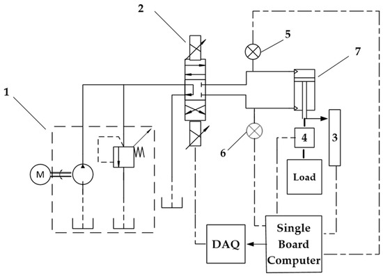
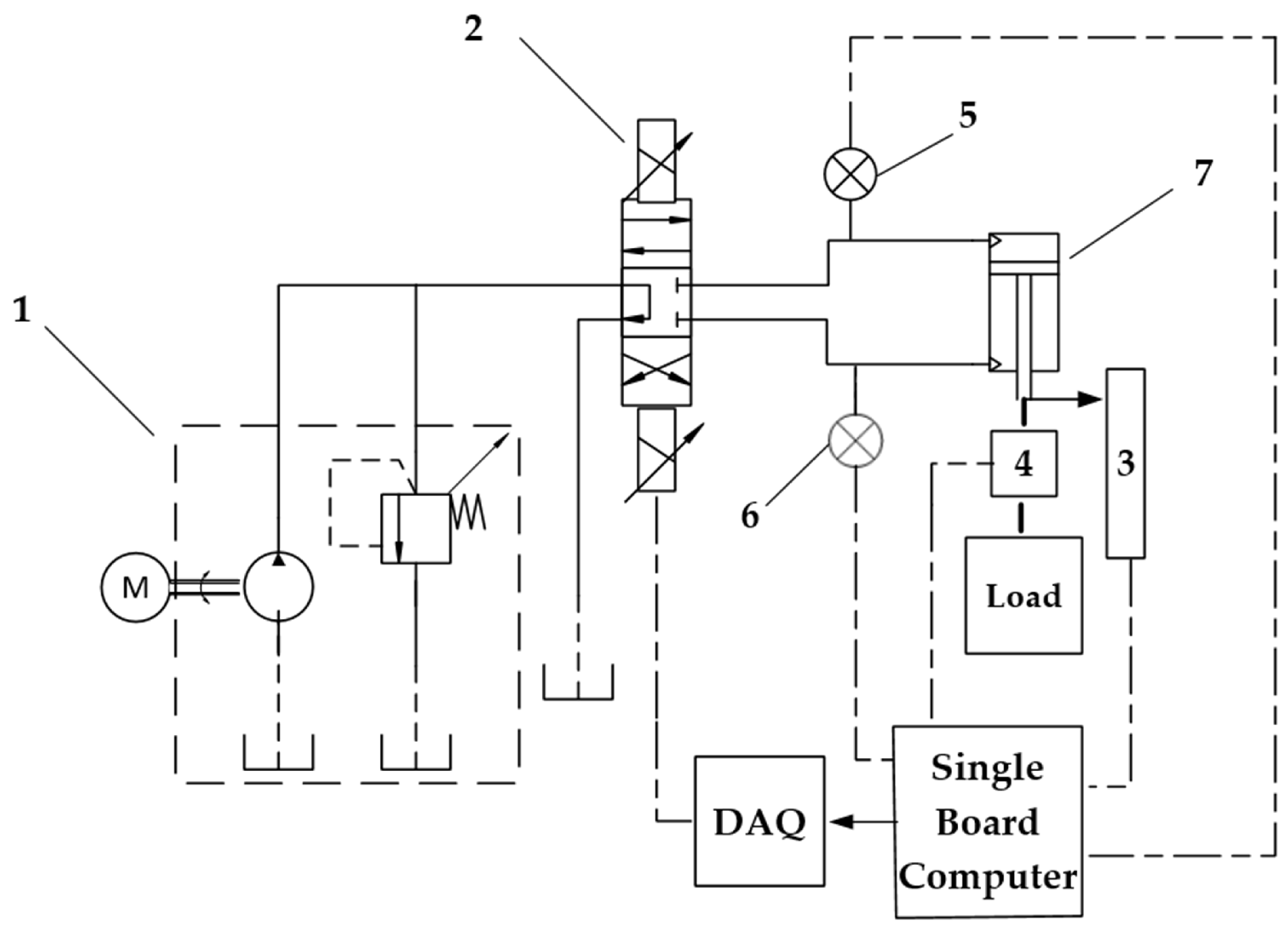
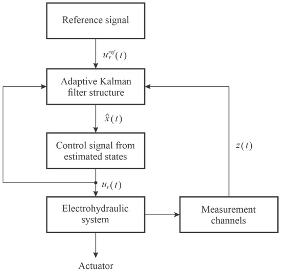
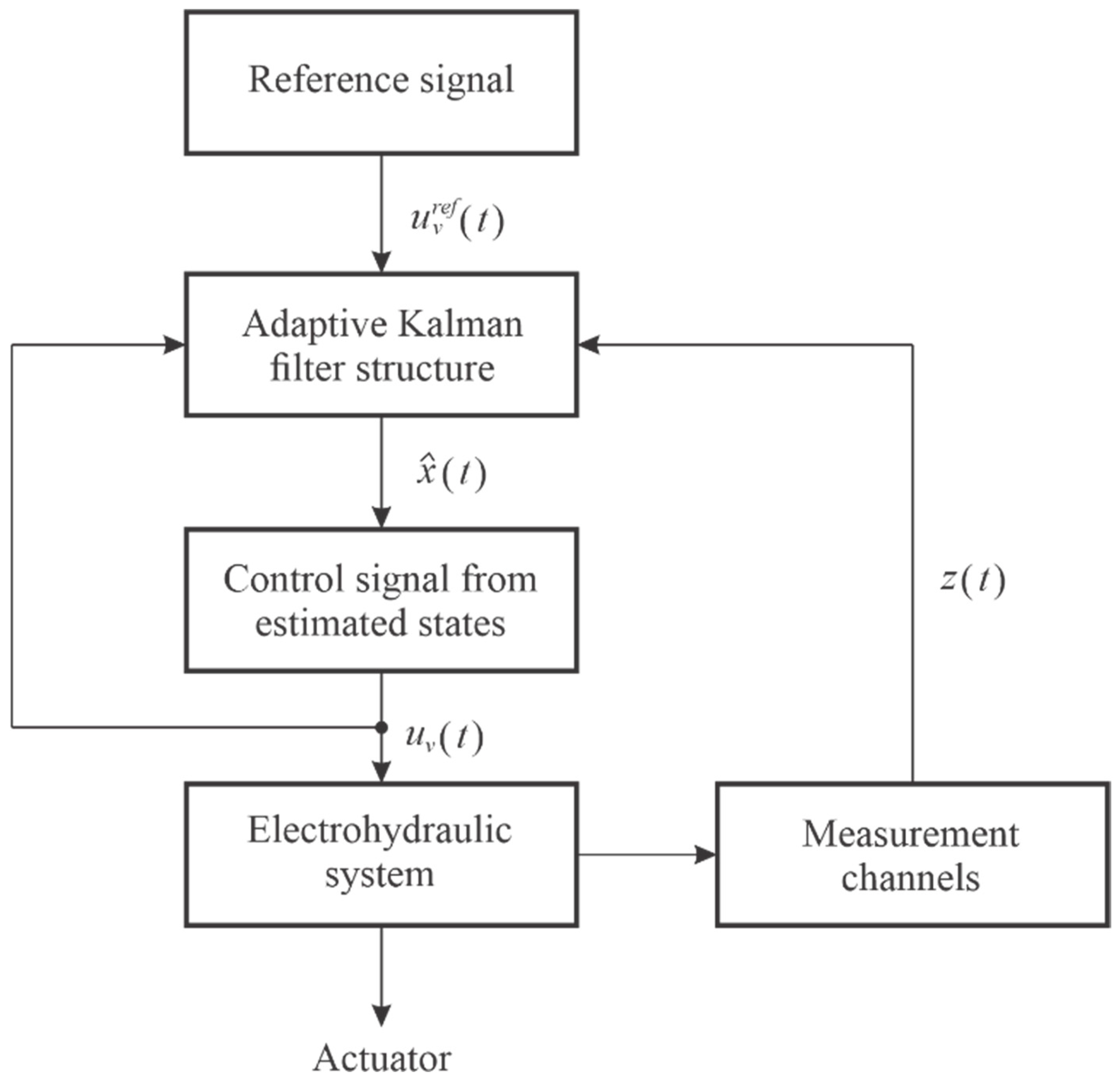
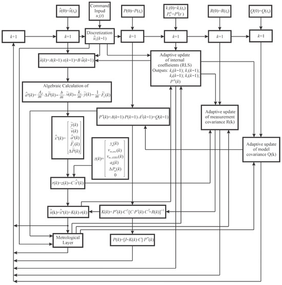
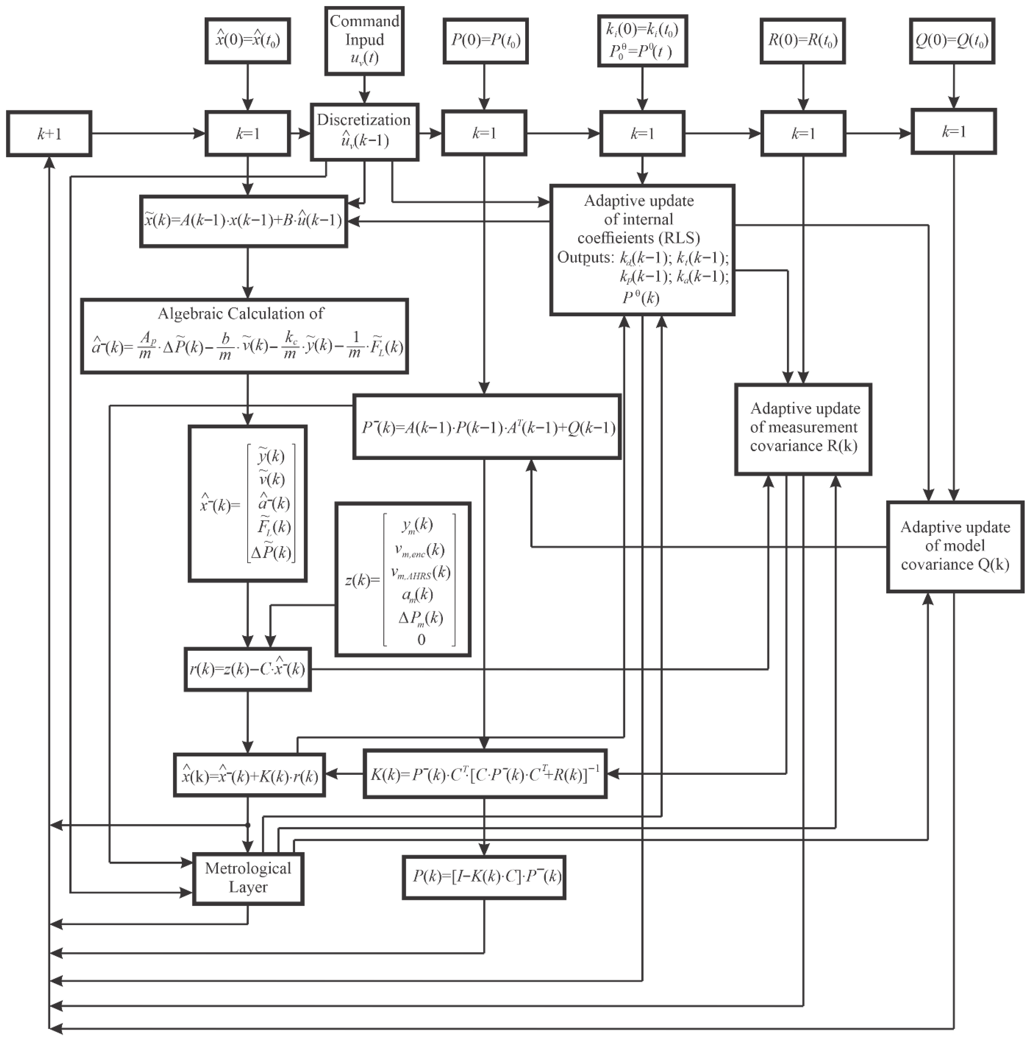
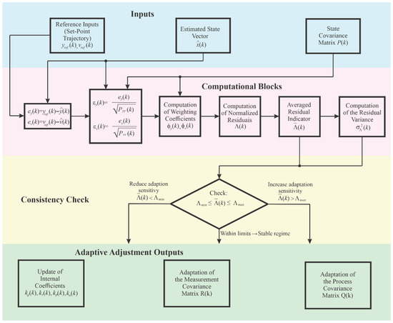
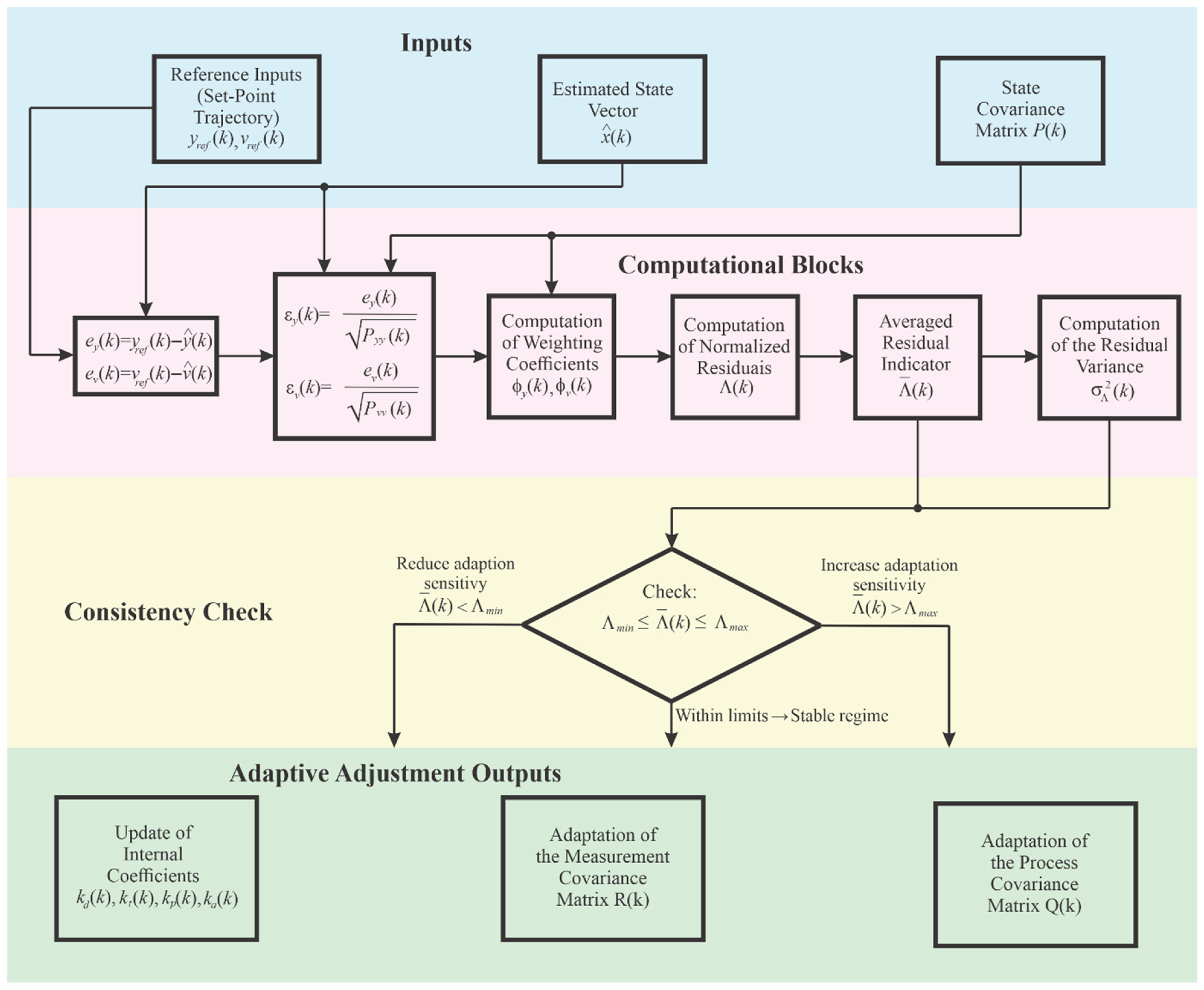
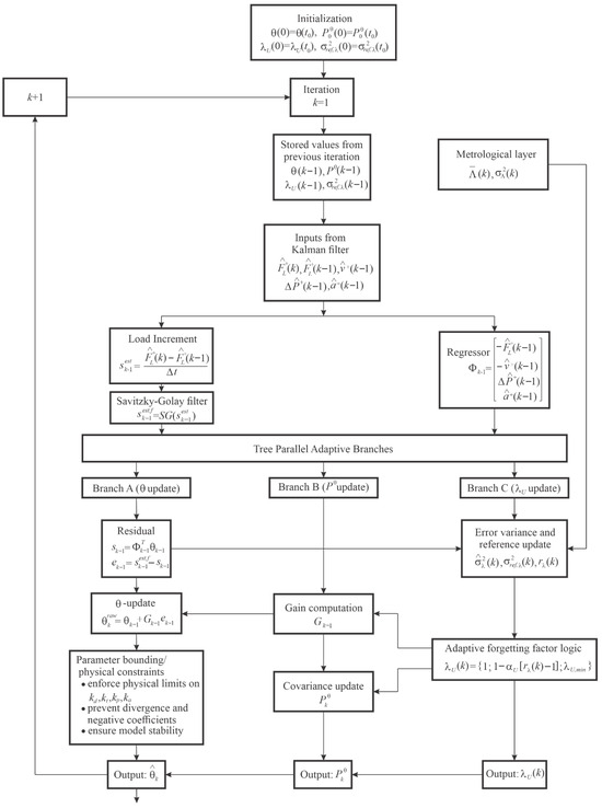
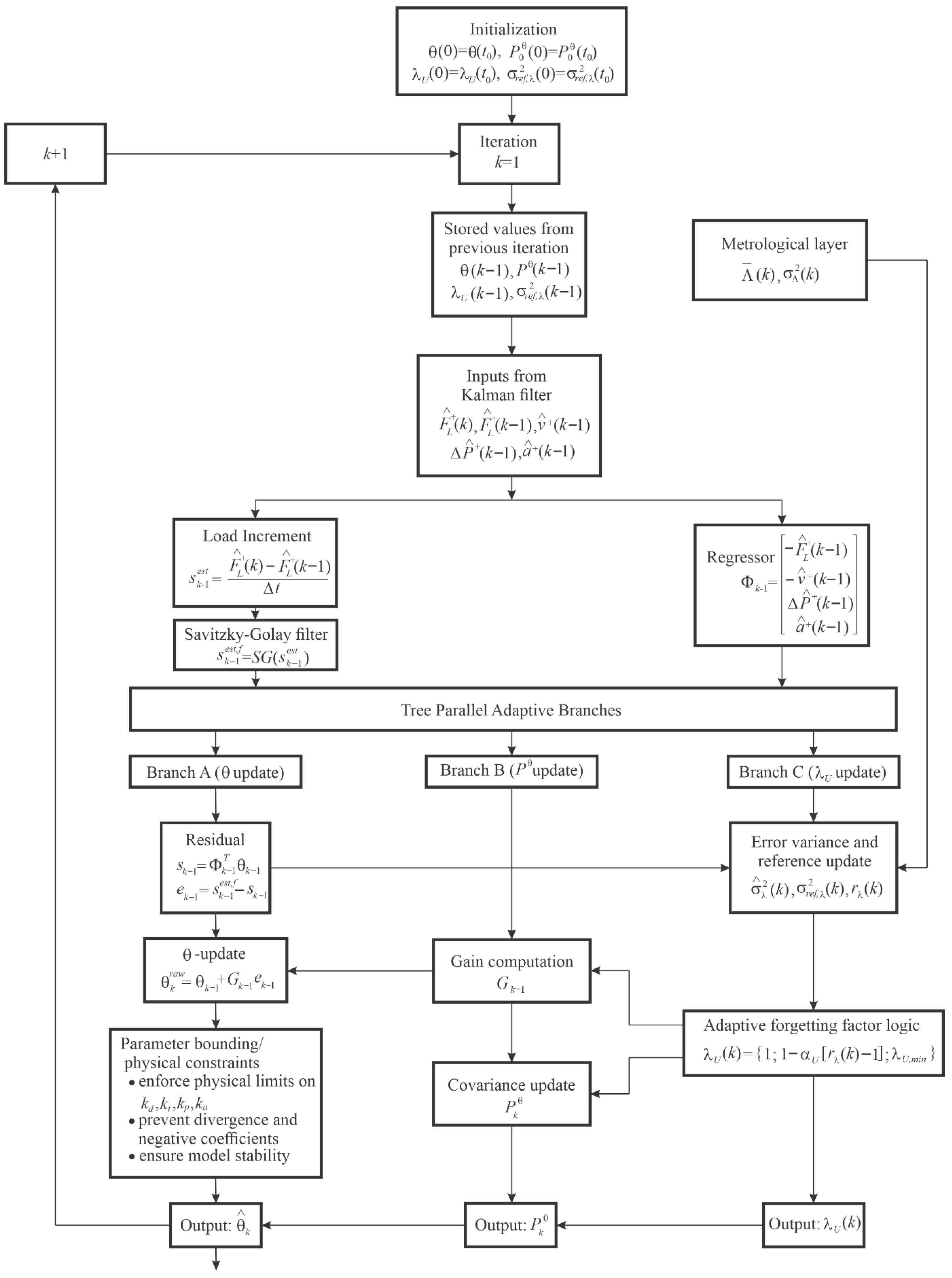
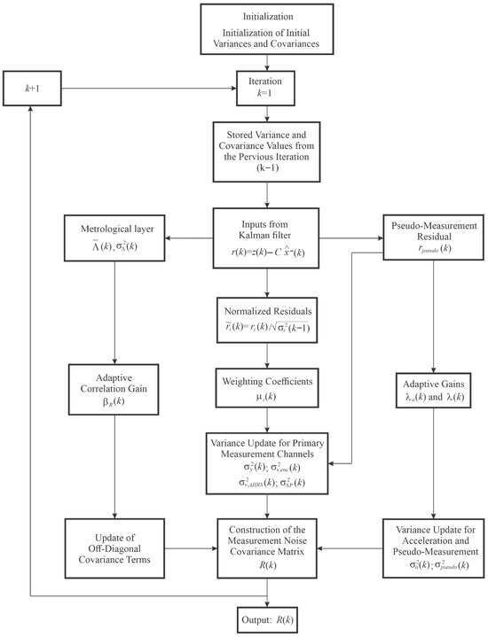
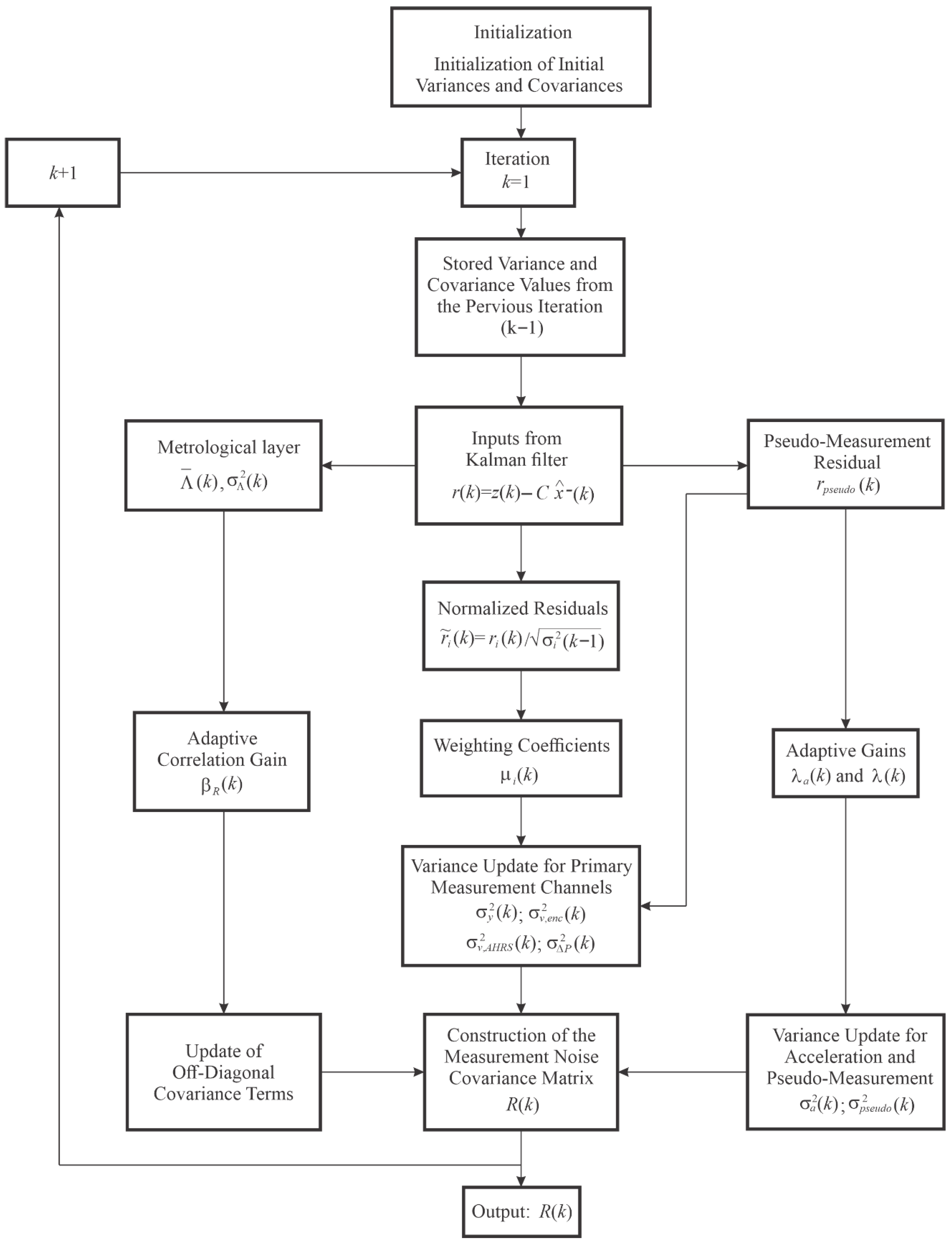
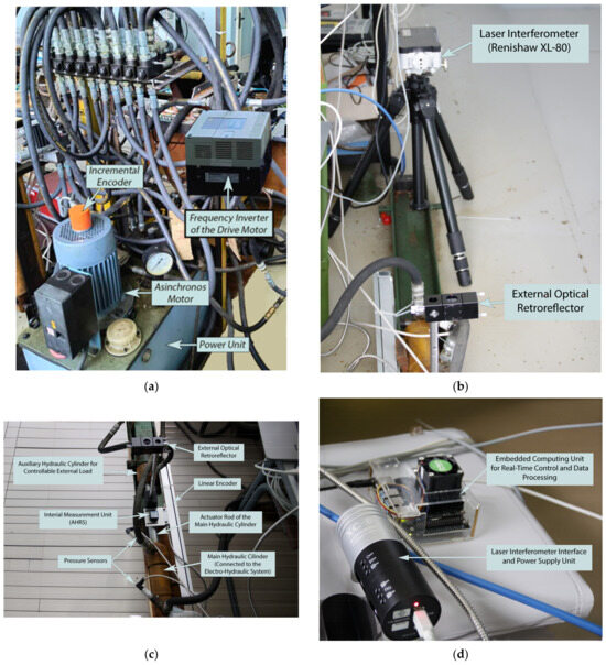
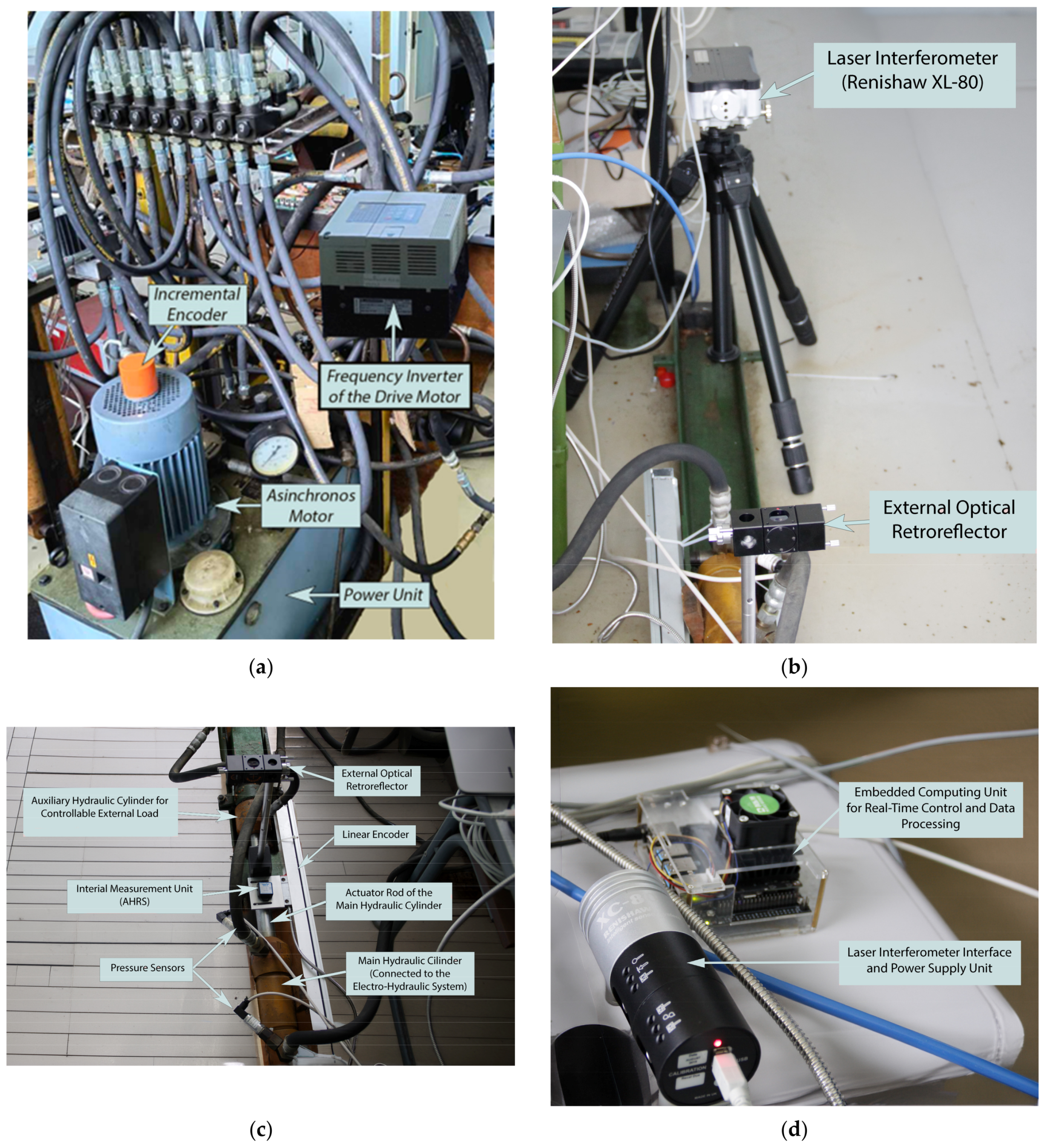
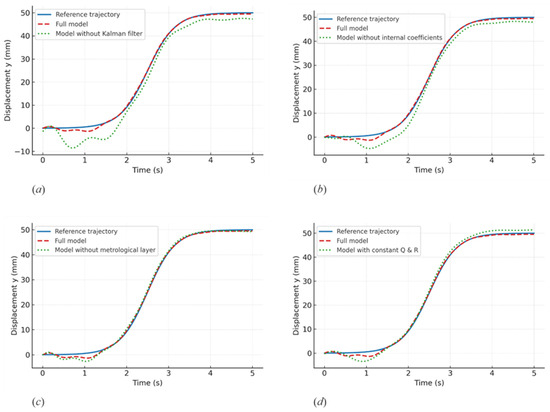
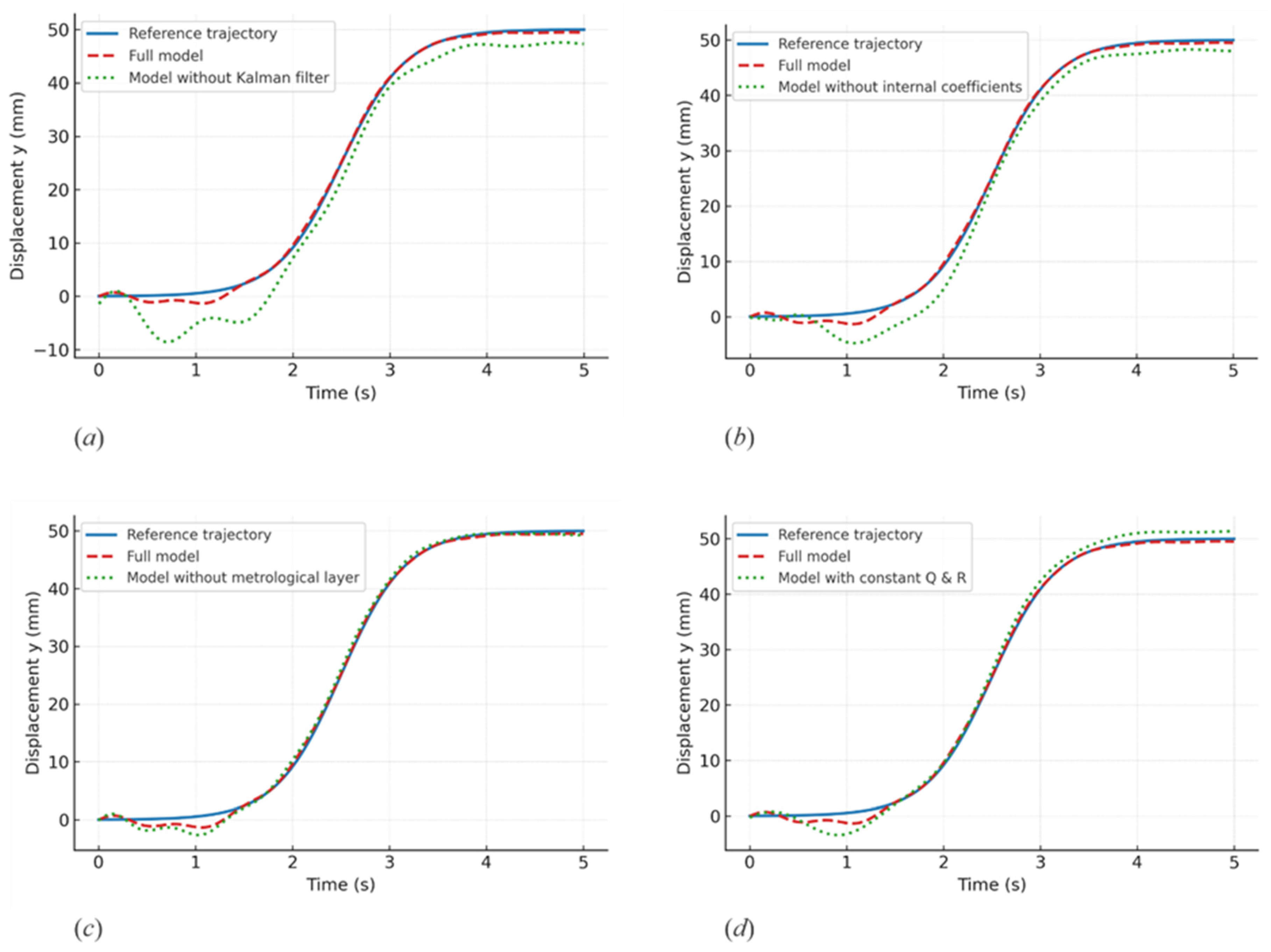
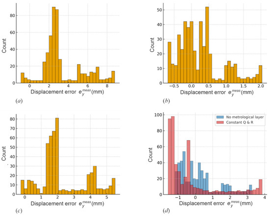
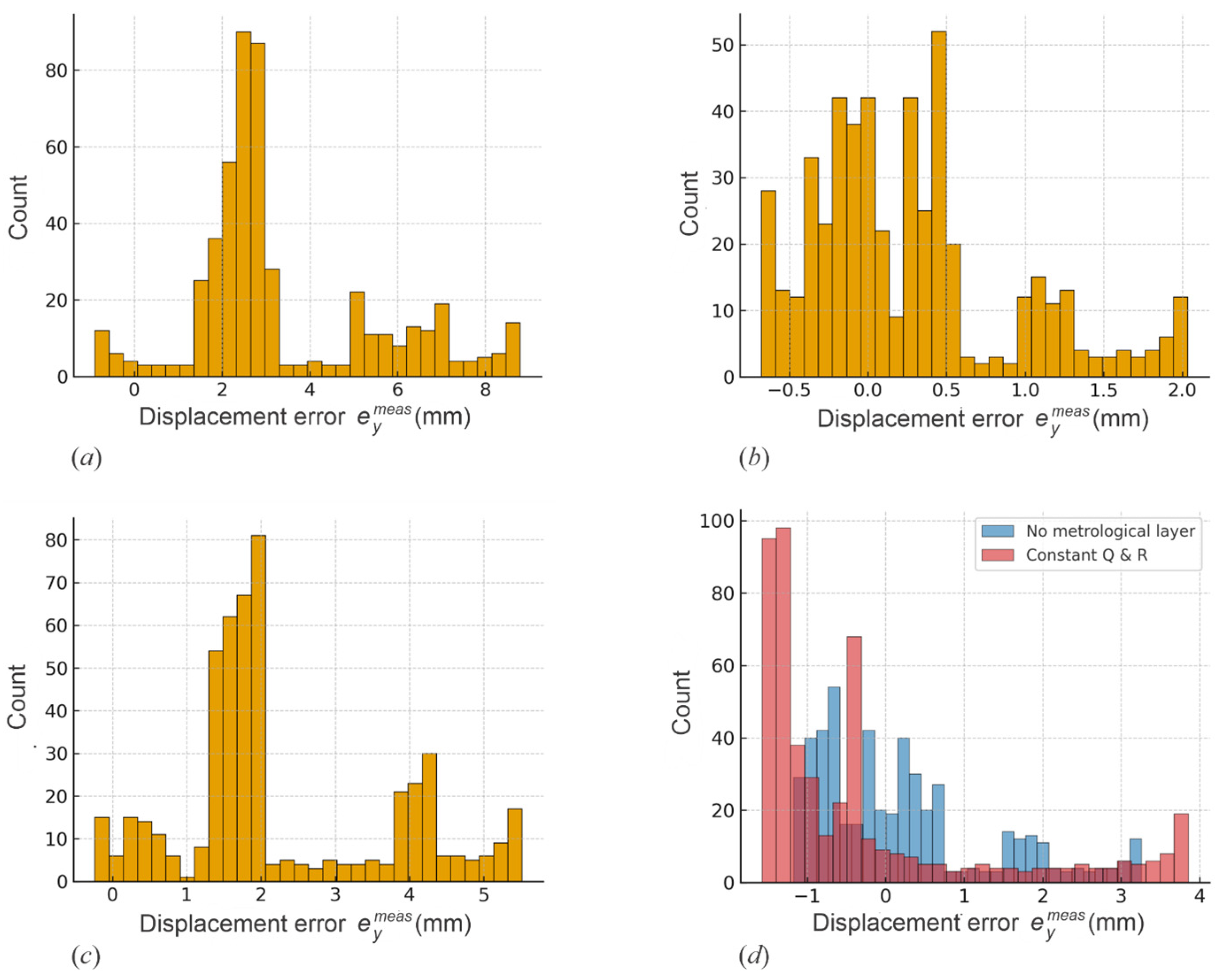
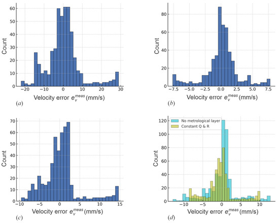
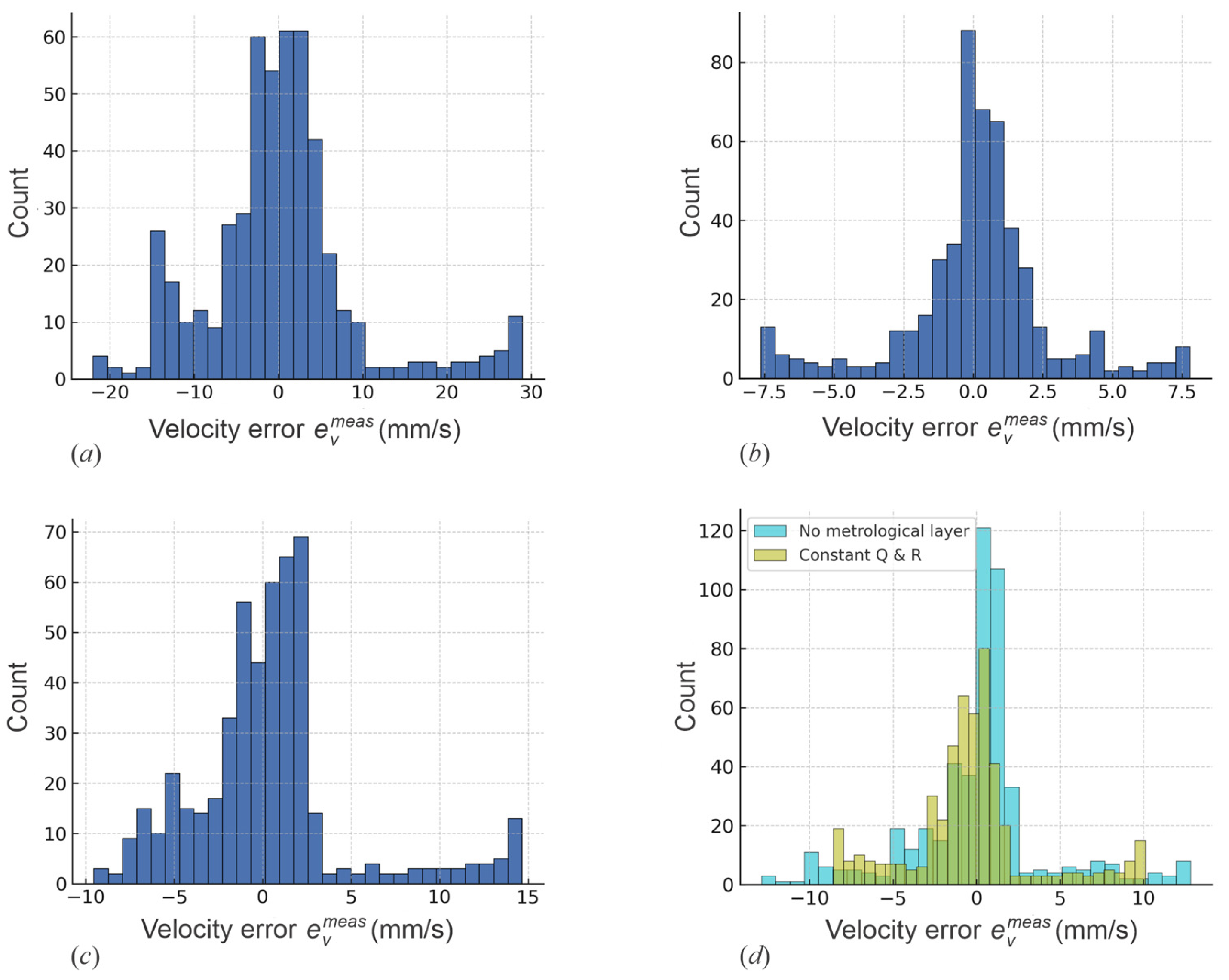
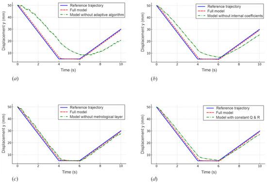
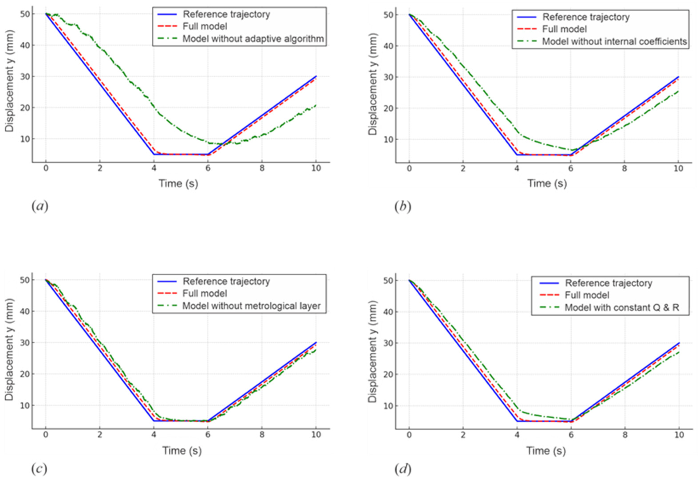
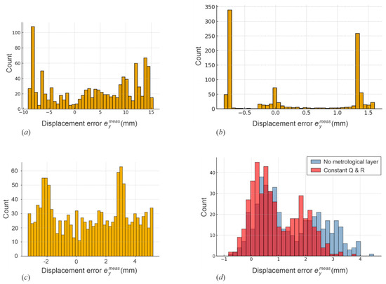
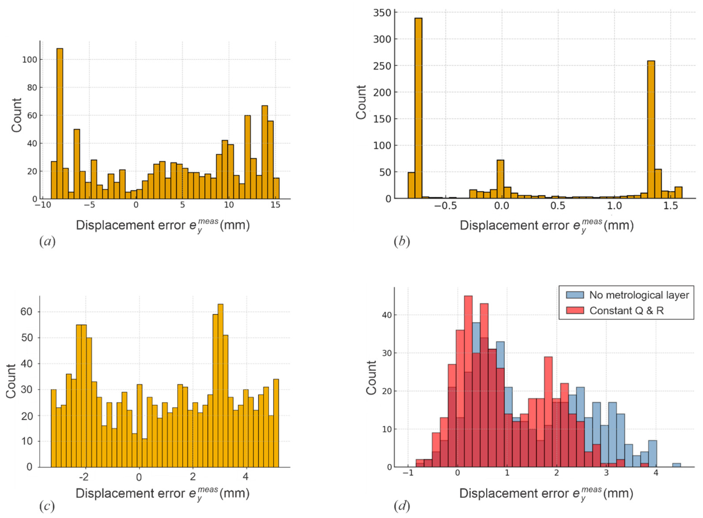
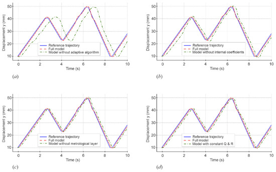
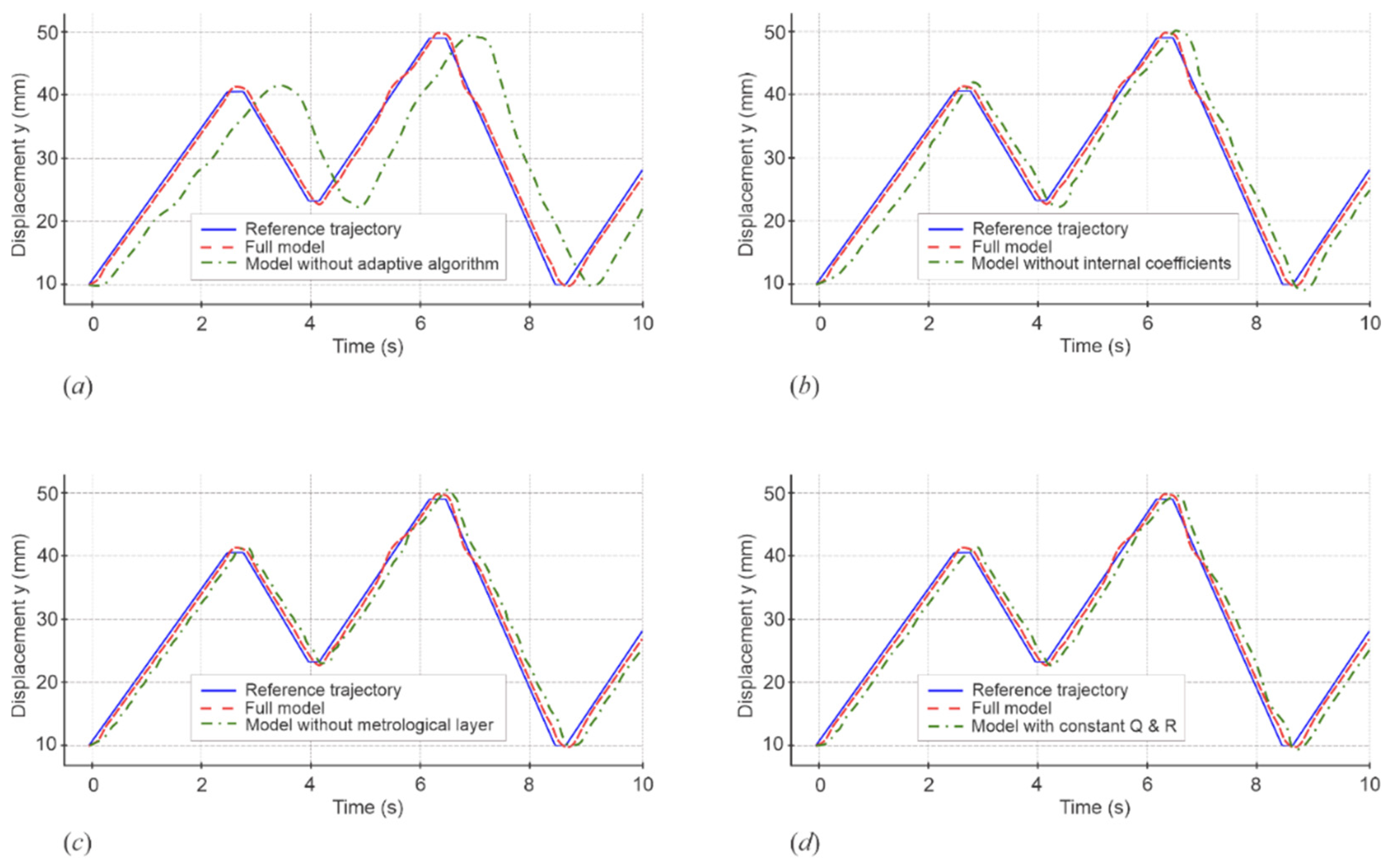
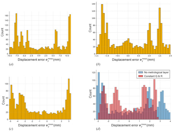
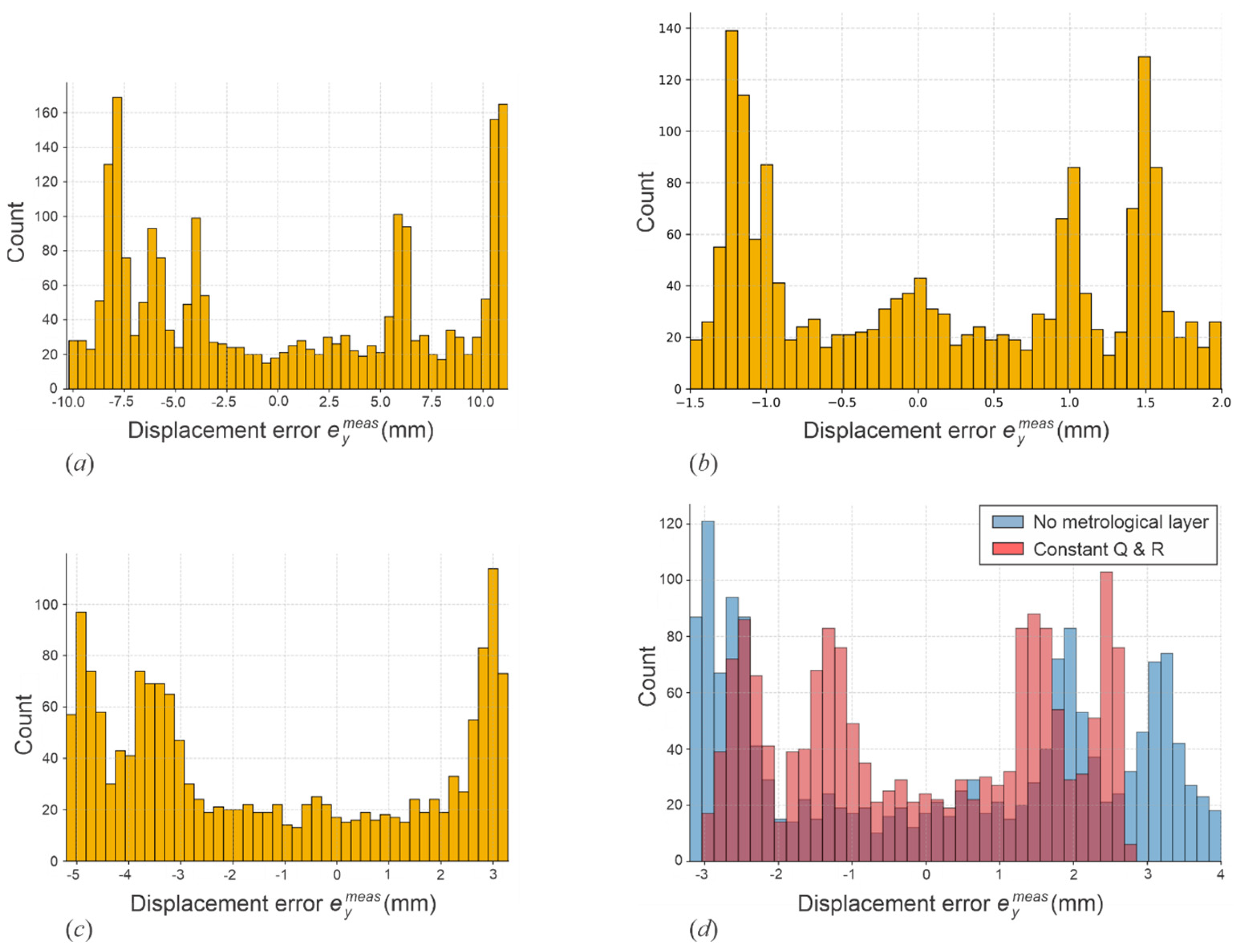
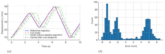
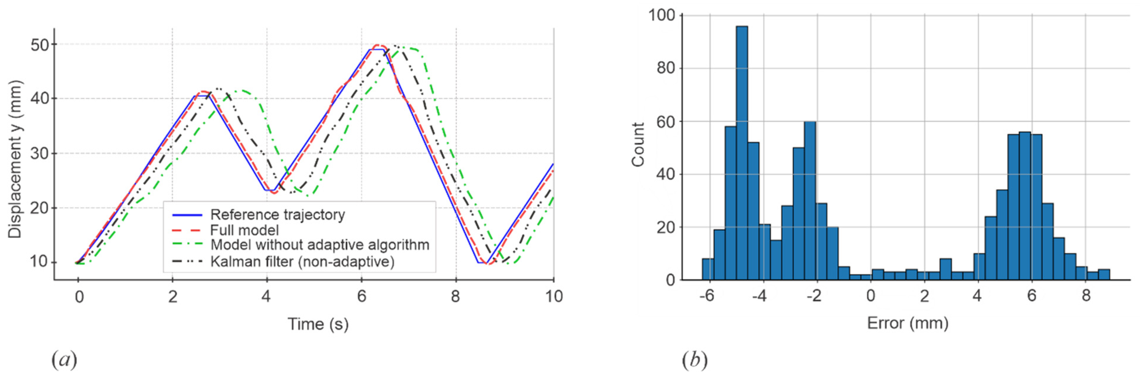

Disclaimer/Publisher’s Note: The statements, opinions and data contained in all publications are solely those of the individual author(s) and contributor(s) and not of MDPI and/or the editor(s). MDPI and/or the editor(s) disclaim responsibility for any injury to people or property resulting from any ideas, methods, instructions or products referred to in the content. |
© 2026 by the authors. Licensee MDPI, Basel, Switzerland. This article is an open access article distributed under the terms and conditions of the Creative Commons Attribution (CC BY) license.