


Abstract
To address the challenges of coordinated optimization in building integrated energy systems (IES) under the dual-carbon targets—characterized by strong multi-energy coupling, significant uncertainty in renewable generation, and stringent safety constraints—a novel safe deep reinforcement learning algorithm, Safe-DDPG, is proposed. Traditional deep reinforcement learning methods often suffer from high constraint-violation risk and limited policy reliability due to coupled objectives in building IES optimization. To overcome these limitations, a dual-channel critic architecture is designed to independently evaluate and decouple economic and safety objectives. In addition, a dynamic safety–penalty mechanism based on logarithmic barrier functions is introduced, together with an adaptive exploration strategy, enabling dynamic balancing between economic cost and constraint satisfaction according to system states during training. Experimental results demonstrate that, compared with mainstream algorithms, Safe-DDPG achieves substantial improvements across multiple key performance indicators: safety violations are reduced by up to 96.7%, average daily operating costs decrease by 18.5%, and cumulative rewards increase by more than 30%. Ablation studies further confirm the effectiveness and necessity of each core component. Two DRL methods from reference papers are reproduced, and their performance is compared with the proposed method in the existing experimental results, showing that the proposed method has significant advantages in reward value and economic cost. This work provides a safe, reliable, and efficient reinforcement-learning-based approach for optimization and scheduling of building energy systems under complex operational constraints.
1. Introduction
Driven by the global “dual-carbon” strategy, the low-carbon transition of the energy mix has become an inevitable trend of societal development. As one of the major energy-consuming sectors, the building industry contributes over 40% of total carbon emissions, making energy conservation and emission reduction in building energy systems a critical pathway toward achieving carbon-neutrality goals. Integrated Energy Systems (IESs) [1], which combine photovoltaic generation, wind power, energy storage, heat pumps, combined heat and power (CHP) units, and other heterogeneous devices, enable the coordinated optimization of electricity, heating, and cooling flows. Consequently, IESs [2] are widely recognized as a key technological route for improving building energy efficiency and facilitating deep decarbonization.
However, the optimal operation of building-level IESs presents significant challenges. The system features strong nonlinear coupling among multiple energy carriers (electricity, heating, cooling) [3]; renewable generation and load demand exhibit substantial uncertainty [4]; and strict physical constraints—such as state-of-charge limits of energy storage, equipment operating boundaries, and grid-interaction restrictions—must be satisfied to ensure operational safety. Violations may cause equipment degradation, system failures, or even threaten grid security. These three core challenges collectively render the energy management of building-scale IESs a multi-objective optimization problem in which economic efficiency, operational feasibility, and system safety must be simultaneously guaranteed.
Fundamentally, IES energy management is a complex, nonlinear, multi-objective optimization problem. In practical applications, energy production and consumption exhibit continuity, discreteness, and high uncertainty, further increasing the difficulty of optimization. To address these challenges, a wide range of methods has been explored, which can be broadly categorized as follows:
- (1)
- Mathematical Analysis (MA) methods. Mixed-Integer Linear Programming (MILP), nonlinear programming, and integer programming are commonly used approaches. For example, ref. [5] applied MILP modeling to optimize community-level energy management; ref. [6] introduced a distributed coordination strategy based on the alternating direction method of multipliers (ADMM); and ref. [7] employed game-theoretic formulations to enhance scheduling flexibility. MA methods provide a rigorous theoretical foundation and solve small- to medium-scale deterministic problems efficiently. Nonetheless, as system size grows and multi-dimensional uncertainties intensify, their computational burden increases sharply, often resulting in local optima or infeasible solutions within acceptable time limits.
- (2)
- Swarm Intelligence optimization (SIO) methods, Genetic Algorithms (GA), Particle Swarm Optimization (PSO), and Ant Colony Optimization (ACO) have been widely applied in IES due to their simplicity, ease of implementation, and strong global search capability. These methods show better robustness [8] and global exploration capability than classical mathematical programming. However, their computational effort grows exponentially with problem dimension, and optimality cannot be guaranteed. They also suffer from long computation times [9] in large-scale IES scenarios.
- (3)
- Data-driven artificial intelligence methods. With the growing deployment of sensors and metering devices, data-driven approaches have been increasingly adopted in IES energy management. Reinforcement learning (RL), which does not rely on precise system models and learns optimal scheduling policies through environment interaction, has emerged as a promising solution for complex and uncertain energy systems. In particular, RL provides inherent advantages in Multi-Agent Energy Management (MA-EM) [10], offering adaptability and continuous learning capabilities that traditional model-based approaches lack.
- (4)
- Deep Reinforcement Learning (DRL) methods. To handle high-dimensional state and action spaces, RL has evolved toward deep reinforcement learning, which has shown substantial potential in IES optimization. Existing DRL-based studies primarily fall into two directions: physical system modeling, including day-ahead scheduling under uncertainty [11], robust scheduling under stochastic wind generation [12], carbon-trading-aware energy optimization [13], and peer-to-peer energy trading in multi-energy microgrids. For example, ref. [14] utilized Multi-Agent Twin Delayed Deep Deterministic Policy Gradient (MATD3) to optimize real-time energy trading and conversion strategies in multi-energy microgrids; ref. [15] proposed a DRL-based scheduling approach for hydrogen-incorporated IESs under joint constraints of carbon trading and electricity market operations. Algorithmic development, covering Q-learning, Deep Q-Network (DQN), Deep Deterministic Policy Gradient (DDPG), Proximal Policy Optimization (PPO), and their variants, which have been applied to energy storage scheduling [16] and electricity–heating–cooling co-optimization. For instance, ref. [17] employed DDPG to address multi-objective optimization of electricity–heat–gas IESs and enhanced exploration using an Ornstein–Uhlenbeck process; ref. [18] applied an improved DRL method to manage high-coupling, multi-constraint uncertainty in dynamic energy scheduling; ref. [19] used an improved Twin Delayed Deep Deterministic Policy Gradient (TD3) algorithm to optimize regional IESs operation under multiple uncertainties.
Despite the promising potential of DRL for IES energy optimization, several limitations remain.
- (1)
- Most existing studies aggregate multi-objective reward signals into a single scalar using weighted summation, which often results in objective dominance or objective vanishing due to inconsistent magnitudes, thereby failing to accurately capture the trade-offs among economic efficiency, operational safety, and environmental performance.
- (2)
- Multi-objective outcomes are not directly observed during training, leading to limited interpretability and insufficient safety guarantees of the learned scheduling policies.
- (3)
- Current approaches typically focus on single-task optimization and lack the capability to learn and generalize from multiple perspectives simultaneously.
These limitations highlight the urgent need for multi-objective DRL frameworks that can integrate physical knowledge with the advantages of reinforcement learning, enabling interpretable, safe, and efficient energy management strategies. Although prior studies have explored multi-objective DRL in the energy domain, most still rely on weighted reward functions, which fundamentally fail to overcome the aforementioned issues. Two major limitations persist in existing DRL-based approaches: multi-objective properties—such as economic cost, safety constraints, and carbon emissions—are typically combined through weighted summation, resulting in weight-sensitive optimization outcomes, limited robustness [20], and inaccurate characterization of cross-objective trade-offs. Safety constraints are commonly handled by inserting penalty terms into the reward function; however, such posterior penalties are insufficient to guarantee strict constraint satisfaction during training. This may lead to violations such as energy storage SOC boundary breaches or equipment overload, posing potential operational risks.
For example, ref. [21] adopted a constrained RL approach to handle multi-objective coordination and strict physical constraints in dynamic IES scheduling. In [22], an enhanced DRL method was proposed to simultaneously satisfy long-term energy supply continuity, data transmission performance requirements, equipment operating limits, and multi-objective constraints in integrated data–energy systems. In [23], robustness assessment and enhancement techniques were introduced to improve the resilience of DRL-based load restoration strategies under uncertainty.
As shown in Table 1, existing IES optimization methods struggle to balance decoupled multi-objective optimization, strict constraint handling, dynamic uncertainty adaptability, and engineering-level computational efficiency. Mathematical analysis and swarm intelligence optimization are restricted by static features and high computational complexity, incompatible with high-dimensional and dynamic IESs operation. Traditional DRL solves dynamic modeling issues but causes objective imbalance via weighted aggregation, with static penalty failing to ensure operational safety. Traditional MO-DRL achieves preliminary multi-objective decoupling yet lacks strict hard constraint handling and dynamic adaptability to strong IESs uncertainty.
Table 1.
Comparison of research status of IES optimization methods.
In this context, this paper proposes a multi-objective deep reinforcement learning [24] method for optimizing building-level Integrated Energy Systems, addressing the challenges of conflicting objectives and stringent safety constraints. The method integrates value-decomposition and policy optimization mechanisms to decouple economic and safety objectives, overcoming the limitations of traditional weighted-sum approaches that often lead to objective imbalance or vanishing effects. The key contributions are summarized as follows.
- (1)
- A multi-objective, safety-aware deep reinforcement learning framework tailored for building IESs is proposed. By introducing dual critic networks in the Actor–Critic architecture, economic and safety objectives are separately evaluated, effectively preventing the objective imbalance caused by conventional weighted reward formulations.
- (2)
- A combination of logarithmic barrier functions and adaptive penalty coefficients is designed to enforce strict safety constraint satisfaction while optimizing economic performance. Through value function decomposition and reconstruction, the proposed method ensures explicit and independent representation of economic and safety objectives throughout the training process.
- (3)
- The proposed framework provides a flexible approach for capturing the complex coupling between economic efficiency and operational safety in building IESs. It enables the Safe-DDPG architecture to achieve coordinated optimization under uncertain environments, offering improved feasibility and robustness.
The remainder of this paper is organized as follows. Section 2 formulates the multi-objective optimization model for building IESs. Section 3 describes the Markov decision process formulation. Section 4 introduces the architecture and algorithmic design of the proposed Safe-DDPG framework. Section 5 presents simulation experiments and results analysis. Section 6 concludes the paper and discusses potential future research directions.
2. Overall Design of Building IES
This section develops a multi-objective optimization framework tailored for building-level IESs under dual-carbon targets, with a particular focus on the coordinated optimization of economic performance and operational safety. The framework incorporates energy-supply device modeling, multi-energy flow balance analysis [25], and explicit safety constraint formulation. Through mathematical modeling, key factors—such as photovoltaic generation variability, load demand uncertainty, and device operational limits—are quantified to provide clear problem boundaries and optimization objectives for the subsequent deep reinforcement learning-based solution.
2.1. Architecture and Operational Mechanism of Building IESs
This study addresses the energy consumption optimization problem in building-level IESs, aiming to minimize operating costs while maintaining the supply–demand balance among electricity, heating, and cooling, as well as satisfying equipment safety constraints. The building IES integrates three subsystems: energy supply, energy conversion, and demand-side loads. It consists of photovoltaic (PV) generation, wind power generation, battery energy storage, combined heat and power (CHP) units, gas boilers, heat pumps, and electric chillers. Its operation is affected by electricity prices, load demand variations, and renewable generation uncertainty. Figure 1 illustrates the interaction architecture of the building IES, highlighting the coupling among electricity, natural gas, cooling, and heating flows. The system meets complex load requirements through energy conversions carried out by various devices. The functions and modeling of each subsystem are described as follows.
Figure 1.
Framework of the building Integrated Energy System.
- (1)
- Energy Supply Subsystem
The energy supply subsystem is built upon multi-source coordination, integrating clean generation, backup supply, and storage flexibility to ensure stable and low-carbon energy input. PV generation serves as a primary clean energy source and is modeled via a data-driven simplified formulation:
where is the PV output at time (kW), is solar irradiance (kW/m2), is the conversion efficiency, and is the effective area (m2).
Wind power generation is modeled through a wind-speed-to-power mapping function:
where is the wind power output at time (kW), is the real-time wind speed (m/s), and denotes the turbine power curve.
Grid interaction functions as a bidirectional interface that supports both electricity import and export. It compensates for renewable generation shortages and enables surplus electricity to be injected into the grid. The variables and denote the purchased and sold power at time (kWh), respectively.
Energy storage consists of battery storage and thermal storage tanks. Battery storage is constrained by its dynamic state-of-charge (SOC) model:
where is the SOC at time (%).
Thermal storage is governed by its heat accumulation model:
where represents the thermal storage level at time (%), and , denote charging and discharging efficiencies. Storage components collaboratively perform temporal shifting of electricity and heat, alleviating supply–demand mismatch.
- (2)
- Energy Conversion Subsystem
The energy conversion subsystem transforms and allocates electricity, heating, and cooling through precisely modeled devices, ensuring accurate energy conversion efficiency and supply–demand matching.
The CHP unit acts as the core multi-output device and is modeled using nonlinear natural gas input–output relationships:
where is natural gas consumption (m3/h), and , are the electrical and thermal efficiencies calibrated using real operational data.
Heat pumps and electric chillers convert electrical energy into heating and cooling, respectively:
where and are the coefficients of performance, which vary temporally with outdoor temperature.
- (3)
- Load Subsystem
The load subsystem represents the demand side of the system, requiring accurate modeling of electrical, thermal, and cooling loads. Annual hourly load profiles derived from historical monitoring data are used to characterize seasonal and temporal demand patterns.
In practice, an energy hub aggregates multiple building-level IESs units into a coordinated system, enabling centralized scheduling and decentralized execution. External energy sources—such as electricity and natural gas—are distributed to individual subsystems according to the optimized energy management strategy. Each building IES functions as an independent decision-making entity that must consider both local operating costs and safety constraints while responding to allocated energy resources.
Based on this structure, the next section formulates the multi-objective optimization model for the building IESs, defining the objective functions and constraints required to ensure economically efficient and safely constrained system operation.
2.2. Multi-Objective Optimization Model for Building IES
The multi-objective optimization model for the building IES is formulated to achieve rational allocation of externally supplied energy within the system. The objective is to accurately distribute the purchased energy to the electricity, heating, and cooling subsystems according to real-time building demand, while simultaneously optimizing the operational scheduling of internal devices—such as CHP units, energy storage, and heat pumps—to ensure efficient and stable energy utilization.
From the perspective of model design logic, the fundamental requirement is to satisfy the building’s basic load while constructing an optimization framework that jointly considers economic efficiency and operational safety. On the one hand, refined calculations of energy procurement costs and equipment degradation costs are employed to minimize the lifecycle operational cost of the building IES. On the other hand, safety violations are quantified through risk metrics designed to prevent issues such as battery SOC violations or equipment overloading, thereby ensuring system stability. Notably, system constraints are embedded into the safety-driven objective, where the economic objective focuses on cost minimization and the safety objective emphasizes risk mitigation. Together, these objectives form the core direction of optimization: maximizing economic performance while strictly maintaining safety thresholds.
2.2.1. Objective Functions
The operation of the building IES must satisfy user energy demand while balancing two primary objectives: economic cost minimization and operational safety assurance. To this end, a dual-objective optimization framework is developed, consisting of minimized operation cost and minimized safety violations. A weighted aggregation approach combined with penalty functions is adopted to enhance compatibility with practical engineering requirements. To align with the research norms for solving the Pareto optimal solution set in multi-objective optimization, a convex weighted sum form is adopted to construct the overall objective function, which couples the two sub-objectives of economic cost and operational safety violation. The overall objective is expressed as:
where and correspond to the minimization of operation cost and the minimization of safety violations, respectively. ∈ [0, 1] is defined as the weight coefficient of the economic objective, whose value determines the optimization preference for the dual objectives. Specifically, when →1, the optimization process prioritizes the reduction of the system’s operational cost, with the economic objective playing a dominant role; when →0, the optimization gives top priority to ensuring the operational safety of the system, and strictly restricts equipment operation and multi-energy flow balance constraints; when = 0.5, the economic and safety objectives are considered equally important in the optimization process. By adjusting the value of , a series of optimization solutions under different objective preferences can be generated, which lays a rigorous mathematical foundation for the subsequent solution of the Pareto optimal solution set and the trade-off analysis between economic efficiency and operational safety. Their detailed formulations are provided below.
- (1)
- Economic Objective: Minimization of Operating Cost
The economic objective focuses on controlling the total operating cost during the IES lifecycle, including energy procurement and equipment degradation. The total operation cost is given by:
where represents the electricity exchange cost with the main grid under time-of-use pricing (RMB), denotes the natural gas cost for the CHP unit and gas boiler (RMB), quantifies losses associated with energy storage devices (RMB), including battery degradation and thermal losses in the TES tank.
The electricity exchange cost is computed as:
The fuel cost is expressed as:
The degradation and thermal loss cost is formulated as:
where and denote the electricity purchase and feed-in tariffs at time (RMB/kWh), respectively, represents the unit price of natural gas (RMB/m3). The coefficient refers to the battery degradation factor per cycle, while denotes the simulation time step, corresponds to the thermal loss rate of the TES tank, indicates the state of charge of the TES at time , and represents its rated discharging power (kWh).
- (2)
- Safety Objective: Minimization of Operational Risks
The safety objective quantifies the degree of operational violations through penalty functions, mainly considering equipment over-limits and multi-energy supply–demand imbalance. This ensures that abnormal operation does not lead to supply interruption or equipment damage. The safety objective is expressed as:
where and are penalty coefficients, quantifies equipment limit violations, captures energy flow imbalance.
Equipment violation penalties are defined as:
where , and denote the maximum power generation of the CHP unit, the maximum power consumption of the HP, and the maximum power consumption of the AC (kW), respectively. quantifies the supply–demand deviation of electricity, heat, and cooling multi-energy flows using a quadratic function, which amplifies the penalty for large deviations to ensure the continuity of energy supply (kW). It can be expressed as:
where , , and represent the total supply of electricity, heat, and cooling energy in time period , respectively (kW); , , and denote the corresponding user load demands in the same time period (kW).
2.2.2. Energy Balance Constraints
To ensure the safe and stable operation of the building IES, as well as the reliable performance of equipment and the balance between energy supply and demand, a comprehensive set of multi-dimensional constraints must be strictly enforced. In this study, a rigorous constraint framework is established from three core perspectives: device-level physical characteristics, multi-energy flow balance, and operational safety boundaries. The detailed formulations are provided as follows.
- (1)
- Physical Constraints of Energy Conversion Devices
To maintain all energy conversion and storage units within their rated operating ranges—thereby avoiding overload, performance degradation, or permanent damage—physical constraints are imposed on key components, including the battery energy storage system (BESS), CHP, HP, electric chiller, and TES. Specifically, the BESS must satisfy both charging/discharging power limits and state-of-charge (SOC) bounds to prevent overcharging or deep discharging that may accelerate battery aging or induce safety risks. As one of the central cogeneration units, the CHP is required to meet its power output boundaries and ramp-rate limitations, thereby preventing excessive start–stop events or abrupt load variations that may lead to equipment stress or efficiency fluctuations. The heat pump must satisfy the coupling constraints between heating output and electrical input to guarantee operation within the high-efficiency region. Similarly, the electric chiller must meet the cooling–electricity coupling constraints to avoid inefficient or overloaded operation.
The TES unit, functioning as the thermal buffer, is required to satisfy the constraints on thermal storage level and charging/discharging power to ensure safe and effective thermal energy storage and release. The relevant physical constraints are expressed as follows:
where denotes the battery charging/discharging power at time (kW); and represent the maximum discharging and charging power of the battery, respectively (kW). and denote the electrical and thermal outputs of the CHP unit at time (kW); , , , and specify the corresponding output boundaries (kW); represents the maximum ramping capability of the CHP unit (kW). and denote the heating output and electrical input of the heat pump at time (kW); , , , and define the allowable ranges of heating output and electrical input (kW). and denote the cooling output and electrical input of the electric chiller at time ;, , , and specify the corresponding operating limits. denotes the thermal storage level of the TES at time (kW); and define its allowable storage range (%). represents the charging/discharging thermal power of the TES at time (kW); and denote the maximum charging and discharging thermal power, respectively (kWh).
- (2)
- Multi-Energy Balance Constraints
To guarantee the real-time matching of multi-energy supply and demand within the building IESs, energy balance constraints are enforced for electricity, heating, and cooling. The electrical balance ensures that, at each time step , the total electricity supply equals total consumption, considering renewable generation, CHP output, grid interaction, battery operation, and electrical loads. The constraint is expressed as:
where denotes the PV power generation at time (kW); represents the wind power generation (kW); is the electrical output of the CHP unit (kW); denotes the grid exchange power, with positive values indicating imports and negative values indicating exports (kW); and represent the charging and discharging power of the battery, respectively (kW); denotes the electrical demand (kW); and and represent the electrical consumption of the heat pump and the chiller, respectively (kW).
Thermal balance requires that, at time , the total thermal supply—including CHP heat output, HP heating, and TES discharging—matches the thermal demand and TES charging:
Cooling balance requires that the chiller’s cooling production meets the cooling demand:
- (3)
- Operational Safety Constraints
To avoid voltage or frequency instability caused by excessive power exchange between the building IES and the grid, the magnitude of grid interaction power must be constrained within a safe operating interval. Meanwhile, the stochastic fluctuations in PV and wind output caused by weather variations must be limited to prevent abrupt changes that might affect system balance. The following constraints are imposed:
where and denote the maximum allowable power exported to and imported from the grid, respectively; and represent the maximum permissible variation rates of PV and wind power outputs (kW); and and denote the PV and wind generation levels at time , respectively (kW).
3. Markov Game Model of the Building IES
Section 2 establishes a multi-objective optimization model for the building IES, which can be reformulated as a Markov Decision Process (MDP) for a single intelligent agent. As the decision-making entity, the building IES aims to minimize operational costs while satisfying safety constraints. This objective is achieved by dynamically adjusting the operational strategies of internal devices to maximize its own benefit. The optimal solution corresponds to a stable scheduling policy that balances economic performance and safety requirements. Conventional mathematical programming-based optimization approaches face inherent limitations, such as difficulty in handling uncertainties in PV generation and building loads, reliance on accurate physical models, and the assumption of complete information, making it challenging to leverage historical data for adaptive decision-making.
To transform the multi-objective optimization model in Section 2.2 into a framework amenable to deep reinforcement learning, a Multi-Objective Markov Decision Process (MOMDP) is formulated. Through continual interaction between the agent and the environment—which includes energy markets, load fluctuations, and renewable generation—the model learns an optimal strategy that satisfies multiple objectives. The partially observable decision-making process is characterized by the five-tuple , which incorporates both economic and safety objectives. Here, denotes the state space of the building IES, including key variables such as device operating parameters, storage states, and energy supply–demand conditions. represents the action space corresponding to control commands for major equipment. contains a set of economic and safety rewards, where quantifies operating cost and reflects safety violation risk. describes state transition probabilities that capture the evolution of system states following an action. is the discount factor balancing immediate and future returns. The MOMDP focuses on the decision characteristics of a single IES, removing multi-agent interactions to reduce computational complexity and align the model with practical building energy system operations. The conversion process of the building IES multi-objective optimization problem to the MOMDP is shown in Figure 2. The correspondence between MOMDP elements and actual system variables is summarized in Table 2.
Figure 2.
Conversion process of building IESs multi-objective optimization problem to MOMDP.
Table 2.
Correspondence between MOMDP elements and actual IES variables.
3.1. State Space Design
The state space reflects the real-time operating conditions of a single building IES, including energy supply and demand, device operating states, and storage levels. It must comprehensively capture all dynamic factors influencing IES decisions while ensuring data availability and computational efficiency. Considering the multi-energy coupling of electricity, heat, and cooling, an 18-dimensional continuous state vector is defined as follows:
where is the current time; and represent real-time electricity and gas prices; and denote the battery SOC and thermal storage state; correspond to electric, thermal, and cooling loads; and are PV and wind power outputs; denote the CHP electrical and thermal outputs; are the heat pump electrical consumption and heat output; represent the electric cooling unit power consumption and cooling output; and denote grid import and export power.
3.2. Action Space Design
The action space consists of all controllable variables corresponding to internal device operation commands. It focuses on the key adjustable components of a single IES to ensure smooth device control and avoid abrupt power variations that may lead to equipment degradation. A five-dimensional continuous action vector is defined:
where controls the battery charging/discharging power (positive for charging, negative for discharging), mapped linearly to actual power; controls thermal storage charging/discharging (positive for charging, negative for discharging); regulates the electric cooling unit’s power consumption; adjusts the gas input or electrical output of the CHP unit; adjusts the heat pump input power to regulate heat output.
3.3. Multi-Objective Reward Function Design
The reward design adopts separate economic and safety reward functions to avoid priority imbalance caused by traditional weighted-sum methods. The two-dimensional feedback structure includes an economic reward , which minimizes IES operational cost, and a safety reward , which penalizes violations of operational constraints. Both rewards are formulated as negative values.
- (1)
- Economic Reward
- (2)
- Safety Reward
3.4. State Transition Probability Design
In deep reinforcement learning, state transition probabilities describe how the system moves to the next state conditioned on the current state and action. For the building IES, these probabilities must reflect realistic device dynamics, storage evolution, and uncertainties in renewable generation and loads. Device power states are updated based on action commands and equipment operating constraints. Storage states evolve according to charging/discharging processes; for batteries, SOC transitions account for charging/discharging efficiencies, time steps, and capacity, while thermal storage transitions incorporate efficiency and heat loss. These formulations ensure consistency with physical laws and energy conservation principles.
Section 3 formalizes the multi-objective optimization problem of the building IES as an MOMDP by specifying the state space, action space, multi-objective reward functions, and state transition mechanisms. Through continuous interaction with a dynamic environment, the agent autonomously learns an adaptive scheduling strategy that captures system uncertainties and state-dependent characteristics, ultimately achieving minimum operating cost under safety constraints.
4. Design of the Optimization Framework Based on Deep Reinforcement Learning
Traditional DDPG algorithms exhibit limitations when applied to multi-objective optimization in building IESs, particularly in balancing economic performance and operational safety as well as enforcing hard physical constraints. To address these issues, a Safe-DDPG-based safety control framework is proposed (Figure 3). For clarity, the method is elaborated from three perspectives. First, the paradigm of safety–economy co-optimization in building IESs is defined. Second, a Safe-DDPG architecture integrating value decomposition, constraint embedding, and risk modulation is introduced. On top of the conventional DDPG, this architecture employs a dual-channel Critic network to independently evaluate heterogeneous objectives, while logarithmic barrier functions and adaptive mechanisms are incorporated to enforce safety constraints. This design effectively mitigates the typical DRL problems of objective imbalance and loose constraint satisfaction in safety-critical scenarios, thus providing a systematic solution for reliable and efficient scheduling of complex energy systems. Finally, the dual-channel Critic network, the embedded safety–constraint mechanism, and the adaptive risk–control module are developed to form the complete safety control framework, enabling coordinated multi-objective dispatch under complex physical constraints.
Figure 3.
Enhanced Safe-DDPG framework for safety-constrained control in building IESs.
As shown in Figure 3, the improved Actor–Critic framework operates as follows. The Actor network generates continuous control actions, while the two Critic networks evaluate the policy in parallel using samples stored in the replay buffer. The economic Critic quantifies long-term economic returns—such as energy cost and equipment degradation—producing . The risk Critic focuses on operational hazards such as storage SOC violations and equipment overloading, outputting a quantified safety–risk metric . A collaborative gradient fusion mechanism integrates both evaluations to update the Actor network. Meanwhile, hard physical constraints—such as storage SOC bounds and grid exchange limits—are transformed into differentiable penalty terms through logarithmic barrier functions. An adaptive risk–control module monitors system fluctuations and dynamically adjusts the penalty weight: stronger penalties are imposed during unstable conditions, while economic optimization is prioritized when the system operates safely.
The proposed algorithm is deployed in a building IES environment comprising wind power, photovoltaics, energy storage, and gas-fired units. Through continuous interaction with the environment, the agent performs action generation, device output calculation, constraint updating, economic and risk evaluation, and state transition, thereby embedding physical constraints and economic objectives directly into the training process. This design ensures that Safe-DDPG maintains the sample efficiency of DRL while enhancing decision safety and reliability through hard-constraint embedding and adaptive risk modulation in complex, safety-sensitive energy systems. By defining the problem paradigm, designing the system architecture, and detailing the core modules, this section establishes a Safe-DDPG optimization framework tailored to the multi-objective and constraint-rich characteristics of building IESs.
4.1. Problem Paradigm of Safety–Economy Co-Optimization in Building IESs
The multi-objective optimization of building IESs inherently involves trade-offs under operational constraints, with the core challenges arising from both objective coupling and constraint rigidity. From the objective perspective, the prioritization between economic goals—such as minimizing energy procurement costs and equipment degradation—and safety objectives is not fixed but dynamically dependent on the operating scenario. During peak load periods, ensuring that equipment operates within its power limits takes precedence to prevent supply interruptions due to overloading; under such conditions, safety objectives are prioritized over economic efficiency. Conversely, during off-peak periods, operational stress is reduced, allowing relaxation of non-critical constraints and shifting the optimization focus toward cost reduction through flexible scheduling. Conventional DDPG algorithms, which utilize a single scalar reward function, are ill-suited to accommodate such dynamic priority adjustments, often resulting in suboptimal trade-offs: either safety constraints are violated in pursuit of cost savings, or excessive caution leads to elevated operational costs.
From the constraint perspective, the building IES exhibits heterogeneity in constraint types, which can be classified into hard safety constraints and flexible optimization constraints. Hard safety constraints, such as storage SOC bounds and grid interaction limits, are directly linked to system operational safety. Violations may trigger overcharging or overdischarging of batteries, grid voltage fluctuations, and potentially threaten equipment longevity and grid stability. Flexible constraints, such as energy conversion efficiency, primarily impact economic performance when slightly violated and do not directly compromise system safety. Traditional deep reinforcement learning approaches typically treat all constraints with a uniform penalty mechanism, neglecting their relative importance. Consequently, strict enforcement of hard safety constraints is difficult, and excessive penalization of flexible constraints may distort the optimization trajectory, failing to meet the system’s differentiated control requirements.
Furthermore, environmental uncertainties exacerbate constraint enforcement challenges. Energy supply in building IESs is affected by stochastic factors such as solar irradiance and weather conditions, while demand fluctuates due to human activity patterns and ambient climate variations. These uncertainties continuously shift the system state, imposing high demands on the adaptability of the optimization algorithm. Conventional DDPG methods, relying on fixed exploration strategies and static penalty weights, struggle under such dynamic conditions. Insufficient exploration can trap the algorithm in local optima, preventing the identification of globally optimal schedules that balance economic and safety objectives. Conversely, overly aggressive exploration may breach safety constraints, creating conflicts between operational safety and strategy exploration and reducing practical applicability.
Based on the aforementioned problem paradigm, the Safe-DDPG algorithm is designed to achieve three key objectives: (1) decouple economic and safety objectives through independent evaluation mechanisms, and dynamically adjust objective weights according to system operating scenarios to balance safety and economic efficiency; (2) establish a hierarchical constraint-handling framework, strictly controlling hard safety constraints to ensure system safety, while flexibly optimizing soft constraints to enhance economic performance; and (3) adapt to environmental uncertainties by dynamically tuning exploration intensity and penalty weights, thereby maintaining safety while improving strategy exploration efficiency and generating schedules that closely align with real-world operational requirements of building IESs.
4.2. Safe-DDPG Architecture Design
Building upon the conventional DDPG Actor–Critic framework, Safe-DDPG introduces targeted improvements along three core dimensions: value decomposition, constraint embedding, and risk modulation, enabling effective adaptation to the multi-objective optimization and constraint management requirements of building IESs.
At the base framework level, Safe-DDPG retains DDPG’s inherent strength in handling continuous action spaces, with the Actor network generating continuous control actions. Considering the continuous operational requirements of IES devices, the Actor network output layer employs a tanh activation function to ensure that output actions are precisely mapped to physically feasible ranges—for instance, CHP generation constrained to 0–300 kW, and battery charge/discharge power limited to −100 kW to 100 kW—thereby laying the foundation for safe system operation from the action generation stage.
For value decomposition, Safe-DDPG overcomes the single-Critic limitation of conventional DDPG by employing a dual-channel Critic network, enabling independent evaluation and decoupling of economic and safety objectives. The economic Critic quantifies long-term economic returns for a given state–action pair, assessing performance in terms of energy procurement costs and equipment degradation reduction. The risk Critic predicts safety hazards, providing a probability score for potential violations, such as SOC exceedance or equipment overloading. This parallel, independent evaluation allows Safe-DDPG to optimize economic and safety objectives separately during training, avoiding the target imbalance caused by a single reward function in conventional methods.
In the constraint embedding mechanism, Safe-DDPG implements a dual-pathway approach combining feedforward physical projection with feedback logarithmic barrier penalties, enabling hierarchical and efficient control of hard IES constraints. The feedforward pathway directly projects the Actor-generated raw actions into feasible ranges, preventing severe constraint violations at the execution stage. The feedback pathway applies logarithmic barrier functions, imposing progressive penalties on actions approaching constraint boundaries (e.g., discharging a battery near the 20% SOC lower limit). Penalty intensity sharply increases as the action nears the boundary, guiding the policy to proactively maintain a safe margin.
The risk modulation module further incorporates adaptive weighting and exploration adjustment mechanisms to dynamically balance system safety and policy optimization efficiency. Based on the risk Critic’s predicted violation probability, the algorithm adjusts the weighting between economic and safety objectives in real time: when the violation probability exceeds 70%, the risk Critic’s weight is increased to reinforce safety constraints; when the probability falls below 10%, economic objectives are prioritized. Simultaneously, exploration noise in the Actor network is dynamically adjusted according to environmental uncertainty; in highly uncertain conditions (e.g., extreme weather causing large PV output fluctuations), exploration noise is reduced to prevent safety violations; under stable conditions, noise is moderately increased to enhance global exploration. Table 3 summarizes the key differences between the proposed framework and conventional DDPG architectures.
Table 3.
Major differences between the proposed safe-DDPG framework and traditional DDPG architectures.
Overall, the Safe-DDPG architecture preserves the capability of DDPG to handle continuous action spaces while leveraging multiple modules in a coordinated manner to resolve the shortcomings of traditional algorithms in objective balancing and constraint enforcement, ultimately generating intelligent scheduling strategies for building IESs that satisfy both safety and economic optimization objectives under complex operational constraints.
4.3. Core Modules of Safe-DDPG
4.3.1. Dual-Critic Network Architecture
To meet the stringent requirements of safety-critical scenarios, the core innovation of the Safe-DDPG algorithm focuses on the design of a dual-critic network architecture. This design effectively addresses the limitations of conventional reinforcement learning methods in constraint-driven control tasks. The dual-critic structure consists of two parallel evaluation branches: the economic value evaluation branch, which quantifies the contribution of decision actions to task objectives, and the safety risk evaluation branch, which assesses, in real time, the probability and severity of safety constraint violations during decision execution.
Through the collaborative computation of the two branches, Safe-DDPG can perform multi-dimensional quantification of both economic and safety outcomes for each candidate action. This enables task optimization while satisfying safety constraints, providing an interpretable and quantifiable technical pathway for safety-oriented control of complex dynamic systems. The architecture of the dual-critic network is detailed as follows:
- (1)
- Economic Critic Network
The economic critic network employs a deep neural network to approximate the value function. Its structure is as follows: the input layer receives an 18-dimensional state vector (including real-time electricity price, energy storage SOC, and device outputs; see Section 3.1) and a five-dimensional action vector (covering battery charging/discharging and CHP regulation commands; see Section 3.2), forming a combined feature vector of dimension 23. The network comprises three fully connected hidden layers with 256 and 128 neurons, respectively, using ReLU activation functions. The output layer is a single linear unit that provides the long-term economic value, with smaller values indicating lower long-term operational costs:
where denotes the economic critic parameters, is the ReLU activation, is the concatenation of state and action vectors, and and represent the weight matrices and bias vectors, respectively.
The training objective is to minimize the temporal difference (TD) error, ensuring accurate economic value estimation. The TD loss function is defined as:
where is the replay buffer, is the immediate economic reward, and are the parameters of the target economic critic and actor networks, and is the discount factor. The economic critic primarily evaluates electricity procurement costs, equipment operating losses, and other economic metrics, with a target network used for stabilized training.
- (2)
- Risk Critic Network
The risk critic network is designed to evaluate the probability of constraint violations caused by current actions. Discrete safety violations are transformed into continuous risk values for gradient-based optimization. The input layer is identical to the economic critic, with additional features representing constraint boundaries to enhance risk assessment specificity. The network structure mirrors the economic critic, with three fully connected layers using ReLU activations in hidden layers. The output layer employs a Sigmoid function to map risk values into [0, 1], where 0 represents no risk of constraint violation and 1 indicates certain violation:
where denotes the risk critic parameters and is the constraint boundary feature vector. The training objective minimizes the risk prediction error, with the loss function:
where represents the immediate safety violation measure:
where is the absolute deviation from the safe region for constraint type , including SOC, power limit, and grid interaction constraints, and denotes the risk critic target network parameters.
- (3)
- Dual-Critic Coordination Mechanism
The economic and risk critic networks are coordinated through gradient fusion and risk warnings. Actor network updates integrate gradients from both critics to provide optimized action directions that balance economic performance and safety. A risk-adjusted coefficient is applied to balance the two objectives:
where is the Actor objective, and is dynamically adjusted according to the risk critic output. For example, when , prioritizes economic objectives; when , balances objectives; when , safety is prioritized. Risk thresholds also trigger safety warnings, temporarily reducing exploration noise from 0.1 to 0.02 and activating constraint correction modules.
To ensure the stability and convergence of the Safe-DDPG algorithm, we meticulously configure the learning rates for different network components: the learning rate of the Actor network is set to 6.1035 × 10⁻⁵(equivalent to 2−14), while the Economic Critic network and Risk Critic network in the dual-critic architecture share the same learning rate of 1 × 10⁻³. This parameter setting balances the convergence speed of the policy optimization (Actor) and value estimation (Critic), avoiding the overfitting of the Critic network or the slow convergence of the Actor network. Both the Actor and dual-Critic networks adopt a fully connected structure with three hidden layers, where the number of neurons in each hidden layer is set to 256, 128, and 64 in sequence. The output layer of the Actor network uses the tanh activation function to constrain the action space within the valid range of the building integrated energy system, while the Economic Critic network uses a linear activation function for economic value estimation, and the Risk Critic network uses a Sigmoid activation function to output the violation probability of safety constraints (ranging from 0 to 1).
4.3.2. Safety Constraint Embedding Mechanism
To strictly enforce hard constraints in building IESs, Safe-DDPG implements a layered constraint embedding mechanism combining feedforward physical correction and feedback differentiable penalties, covering device power, energy storage SOC, and grid interaction limits. The feedforward path ensures immediate feasibility of actions, while the feedback path guides long-term policy optimization, creating a closed-loop safety control process.
Feedforward Physical Correction: Actor outputs are projected into feasible domains based on device limits and system safety boundaries. For example, battery charge/discharge is constrained to ±100 kW to avoid overcharging or deep discharge, CHP ramping rates are limited to ±150 kW/h, and grid interactions are bounded to 0–200 kW (purchase) and −150–0 kW (sale). The projection function is:
where is the original action, and is the corrected feasible action.
The feedback differentiable penalty pathway is designed according to the type of constraint, forming a hierarchical multi-level penalty function system. The specific design and the corresponding mapping to constraint types are summarized in Table 4. For hard safety constraints, such as energy storage SOC limits and grid interaction power limits, logarithmic barrier functions (Equation (33)) are used to quantify the degree of violation. These functions impose exponentially increasing penalties near the constraint boundaries, forcing the policy to maintain a safe distance from the limits. For critical operational constraints, such as device power limits and ramp rates, quadratic penalty functions with a dead zone (Equation (34)) are employed. Within the safety margin, no penalty is applied; once exceeded, the penalty increases quadratically with the deviation, balancing constraint strictness with policy flexibility. For flexible optimization constraints, such as energy supply–demand balance, linear penalties (Equation (35)) are applied, where minor deviations incur only a linear cost, preventing excessive penalties from causing significant economic inefficiency. Table 4 presents the classification of constraints and the corresponding penalty function assignments.
where denotes the distance function to the safe boundary for constraint , represents the dead zone for critical constraints, is the linear penalty coefficient for flexible constraints, and quantifies the deviation in energy supply–demand balance.
Table 4.
Mapping between constraint types and penalty functions.
To accommodate environmental uncertainties, a multi-dimensional dynamic adjustment strategy is employed for the penalty weight . First, based on the real-time risk value output by the risk Critic network, the penalty intensity is dynamically scaled using Equation (38), with the baseline weight set to 1.0 and the adjustment coefficient controlling risk response sensitivity. Second, a time decay factor (Equation (39)) is introduced to gradually reduce as the training step increases, facilitating a transition from conservative exploration in early stages to refined optimization in later phases. Additionally, a cumulative constraint violation mechanism (Equation (40)) is designed to accumulate penalty weights for persistent violations within a retrospective window of steps, thereby mitigating the accumulation of systemic risks caused by repeated violations.
where is the initial adjustment coefficient, denotes the decay period, is the cumulative penalty coefficient, and represents the constraint violation indicator function at time step .
4.3.3. Adaptive Risk Control Module
The Adaptive Risk Control Module serves as the core component of the Safe-DDPG algorithm for addressing operational uncertainties in building IESs. Through a three-level closed-loop logic—comprising dynamic risk assessment, safety parameter adjustment, and stability guarantee—the module achieves a dynamic balance between system security and economic efficiency. It takes multi-source operational data as input, employs quantified risk indicators as the basis, utilizes coordinated parameter adjustment as the means, and incorporates stability protection as the safeguard, thereby forming a complete closed loop from risk perception to control execution. The specific implementation logic is as follows:
The Dynamic Risk Assessment Submodule utilizes a multi-source information fusion mechanism to evaluate system risks. Fluctuation characteristics of reward signals are analyzed using a sliding-window statistical method, and the optimal risk level coefficient is determined through grid search, with 0.5 established as the critical threshold. This submodule further constructs three key risk indicators: performance fluctuation risk, quantified by the coefficient of variation of rewards , where and represent the standard deviation and mean of rewards within the window, respectively; constraint violation risk, calculated as the moving average of safety penalties over the past 50 steps, including penalties for equipment exceedances and energy imbalances; and state-boundary transgression risk, measured as the normalized inverse distance sum of key state variables—such as battery state of charge, thermal storage level, and grid interaction power—to their safety boundaries. These three risk indicators are integrated into a comprehensive risk assessment through a weighted summation using coefficients of 0.2, 0.5, and 0.3, respectively.
The risk level-based adaptive regulation strategy comprises three coordinative mechanisms. The safety weight adjustment is implemented through the following formulation:
The baseline value of 1.0 ensures fundamental safety requirements, while the adjustment coefficient of 2.0 is determined through ablation experiments. In the exploration strategy adaptation module, the exploration noise decays linearly with the risk level, while the experience replay sampling weight is biased toward high-risk periods. During high-risk scenarios, the Critic learning rate is reduced and the Actor update frequency is decreased; conversely, under low-risk conditions, learning is activated alongside an optimistic exploration mechanism to enable differentiated responses.
The Stability Guarantee Submodule ensures the robustness of the adaptive process through three dedicated mechanisms. First, an exponential moving average filter is applied to the risk level to mitigate the impact of transient fluctuations on parameter adjustments. Second, a minimum parameter adjustment interval of 50 steps is enforced to prevent policy oscillation caused by frequent parameter switching within short timeframes. Third, when the filtered risk level , an emergency response mechanism is triggered: parameter updates in the risk Critic network are frozen, a predefined safety action library is activated—maintaining battery SOC between 40% and 60%, operating the CHP at base load power, and limiting grid power purchase to within 50% of the rated capacity—while the thermal storage tank level is constrained to remain within the 30–70% safety range. Additionally, a historical state backtracking module analyzes risk level trends using a sliding window approach. If the risk level increases by more than 10% over three consecutive windows, the safety penalty weight is progressively raised in increments of 0.2 until the risk level decreases to .
4.4. Preprocessing of Building Energy Datasets
To ensure the reproducibility of the proposed framework and establish a complete, interpretable pipeline from real-world measurements to digital model inputs and physical control commands, this section details the full data preprocessing workflow, including dimension definition, unit calibration, data cleaning, normalization, state–action encoding, and inverse mapping from network outputs to physical quantities.
4.4.1. Real-World Data Adaptation to Digital Format
The raw input dataset consists of real-time measurements from the building integrated energy system, covering key physical quantities with standard engineering units:
- Electrical, heating, and cooling loads (kW);
- Photovoltaic (PV) and wind turbine power outputs (kW);
- Time-of-use electricity price (RMB/kWh) and natural gas price (RMB/m3);
- Equipment-rated parameters including capacity, efficiency, and operating limits;
- Initial state-of-charge (SOC) for battery energy storage and thermal energy storage (%).
Before being fed into the model, raw data are processed as follows:
- Missing values are supplemented using linear interpolation between adjacent time steps.
- Outliers are identified using the 3σ criterion and replaced by the mean of neighboring valid samples.
- All time-series data are aligned to a 1-h resolution, consistent with the scheduling time step of the building IES.
4.4.2. Data Normalization and Encoding for Model Input
To eliminate dimensional influences and stabilize training, all physical variables are normalized into the range [0, 1] using min–max normalization:
where denotes the original physical value, and , represent the predefined physical lower and upper bounds.
The normalized data are then encoded into the eighteen-dimensional state vector and five-dimensional action vector according to fixed physical–digital mapping rules, as defined in Section 3.1 and Section 3.2. Each dimension corresponds to a unique physical variable with a clear practical meaning and feasible operating range.
4.4.3. Inverse Mapping from Network Output to Physical Commands
The Actor network outputs continuous actions in the range [−1, 1] via the tanh activation function. To obtain executable physical control signals, these digital outputs are converted back to actual device setpoints using linear inverse mapping:
where ∈ [−1, 1] is the network output, and , are the physical operating limits of the corresponding component.
This transformation guarantees that all actions remain within feasible ranges and can be directly applied to real-world building IES scheduling.
5. Experiments and Results Analysis
To validate the effectiveness of the proposed Safe-DDPG algorithm in multi-objective optimization for building integrated energy systems (IESs), this section establishes a realistic building scenario, designs multiple comparative and ablation experiments, and conducts comprehensive analysis from both safety and economic perspectives. Through quantitative metric comparisons and in-depth mechanistic analysis, the core advantages of the algorithm and the necessity of its constituent modules are systematically verified.
5.1. Experimental Design
The IES was simulated using a restricted non-public proprietary building energy dataset obtained through industry–university–research cooperation between Taiyuan University of Technology and Shanxi Construction Investment Group Co., Ltd. The dataset provides complete annual hourly monitoring data for 2022 from buildings in Taiyuan, Shanxi Province, China, including time-series thermal loads, electrical loads, cooling loads, solar irradiance, wind speed, and energy price data with a 1-h temporal resolution. It covers all necessary operation parameters for the building IES (e.g., device capacity, energy conversion efficiency, and constraint boundaries). These time-series data comprehensively characterize the energy supply, equipment operation, load demand, and energy storage status of the integrated energy system. The dataset involves confidential enterprise operation information and is protected by a non-disclosure agreement, so it is not publicly accessible.
The load data comprise actual hourly measurements of electrical, thermal, and cooling loads from the building throughout a full calendar year. Renewable energy generation profiles are derived from measured solar irradiance and wind speed data obtained from local weather stations, with a temporal resolution of one hour and a total simulation period of 365 days. A time-of-use pricing scheme is implemented for electricity, while the natural gas price is set at 0.42 RMB per kWh.
The experiments were conducted on a computing system equipped with an Intel Core i9-13900K CPU (3.0 GHz), 32 GB DDR5 RAM, and an NVIDIA GeForce RTX 4090 GPU. The software environment consisted of Python 3.9, PyTorch 2.1.0, and Gym 0.26.2.
To comprehensively and objectively evaluate the performance of the proposed Safe-DDPG algorithm in terms of operational safety, economic efficiency and training stability, the classic Deep Deterministic Policy Gradient algorithm was set as the core baseline method, with three representative state-of-the-art deep reinforcement learning algorithms selected as supplementary comparative algorithms. To ensure the academic validity of the proposed Safe-DDPG methodology, this study reproduces two deep reinforcement learning-based optimization methods from two benchmark papers. The reproduction strictly adheres to the algorithmic principles, core architectures, and key parameters delineated in the benchmark papers, encompassing the OU-DDPG algorithm from ref. [17] and the improved TD3 algorithm from ref. [19]. All reproduced benchmark methods are evaluated on an identical experimental environment and a self-constructed integrated energy system platform (consistent with the system employed in the original study of this paper) to guarantee a fair comparison with the proposed Safe-DDPG. All algorithms were tested under the identical building IES model and unified experimental framework, and a total of five comparative experiments and one ablation study were designed with the specific configurations as follows:
- Case 1: The proposed Safe-DDPG algorithm for the simultaneous optimization of economic and safety objectives;
- Case 2: The conventional DDPG algorithm (core baseline);
- Case 3: The Proximal Policy Optimization (PPO) algorithm;
- Case 4: The Twin Delayed DDPG (TD3) algorithm;
- Case 5: The Soft Actor–Critic (SAC) algorithm;
- Case 6: The OU-DDPG algorithm reproduced from Reference [17];
- Case 7: The improved TD3 algorithm reproduced from Reference [19].
Ablation Study: Three experimental configurations were established by, respectively, removing the risk Critic network from Safe-DDPG, fixing the safety penalty weight at , and disabling the adaptive exploration mechanism. All other parameters remained consistent with Case 1.
The evaluation metrics encompass three categories: safety, economic efficiency, and training performance. Safety metrics include the severity of safety violations, comprising the number of SOC boundary violations, equipment power exceedance incidents, and emergency intervention triggers. Economic performance is measured by the total annual operating cost. Training performance is assessed through the Critic network loss value, cumulative reward, and convergence behavior.
To ensure the fairness and comparability of the experimental results, the Safe-DDPG algorithm and all comparative algorithms adopted unified basic training parameters and experimental settings, with the key specifications as follows: (1) the mini-batch training size was uniformly set to 1024 (determined via preliminary experiments), which achieves the optimal trade-off between computational efficiency and training stability for the building IES’s eighteen-dimensional state space (electricity/heat/cooling load, energy storage state, renewable energy output, etc.) and five-dimensional action space (CHP unit output, heat pump power, energy storage charging/discharging, etc.); (2) for off-policy algorithms (Safe-DDPG, DDPG, TD3, SAC), the replay buffer capacity was set to 500,000 to store sufficient historical interaction experience, while the on-policy PPO algorithm directly updated the policy with on-policy sampling samples without a replay buffer; (3) the discount factor (γ) was set to 0.995 to emphasize long-term economic and safety benefits in the building IES’s operation; (4) the target network soft update coefficient (τ) was set to 3.90625 × 10⁻³ (equivalent to 2−8) to ensure smooth parameter updates and avoid training oscillation caused by abrupt changes; (5) all algorithms were trained for 500 episodes with 4096 environment interaction steps per episode, and the network parameters were updated eight times repeatedly after each sampling (from replay buffer for off-policy algorithms or on-policy collection for PPO) to fully utilize collected data and improve training efficiency.
In addition, rigorous experimental design constraints were imposed to eliminate the impact of inherent randomness in reinforcement learning training on comparison results and ensure the objectivity and reliability of the algorithm comparisons in Figure 4 and Figure 5; all algorithms adopted an identical network architecture with three fully connected hidden layers (consistent neuron numbers and activation functions for each layer) to eliminate interference from structural differences; each algorithm was independently run for 10 repeated training trials to mitigate randomness from neural network parameter initialization; the average values of these 10 independent results were used to plot the curves in Figure 4 and Figure 5, with error bars added to all curves to intuitively reflect each algorithm’s performance stability during training.
Figure 4.
Variation curve of the dual-path Critic network loss values with training steps for Case 1.
Figure 5.
Variation curves of Critic network loss values with training steps for different reinforcement learning algorithms.
The detailed key hyperparameters of the Safe-DDPG, core baseline DDPG and supplementary comparative algorithms (PPO, TD3, SAC), including network structure parameters, training control parameters, algorithm-specific parameters, and safety constraint parameters, are summarized in Appendix A Table A1. For the core design principles and exclusive parameter settings of each comparative algorithm: DDPG, a classic DRL algorithm for continuous action spaces, adopts the Actor–Critic dual-network architecture (alleviating training instability via experience replay and target network separation) and features direct continuous control action output (well-adapted to building IES equipment scheduling), but suffers from inherent limitations including a single fixed Gaussian noise exploration strategy (prone to local optima) and high hyperparameter sensitivity; in this study, its exploration noise standard deviation was fixed at 0.1, with Actor and Critic network learning rates aligned with Safe-DDPG for fair comparison. PPO, an improved policy gradient algorithm, limits policy update step sizes via the Clip strategy to avoid training collapse, and has the advantages of high training stability and sample efficiency without a replay buffer, but exhibits slightly lower fitting accuracy for continuous action spaces than DDPG-series algorithms; its clip coefficient was set to 0.2, the Generalized Advantage Estimation (GAE) discount factor to 0.95, and an episode update strategy with eight network updates per episode was adopted. TD3, a classic improved version of DDPG, integrates dual Critic networks and delayed policy updates to suppress Q-value overestimation (improving training stability) and introduces target action noise to optimize exploration strategies, with the only limitation of slightly slower training speed than the original DDPG; its target action noise standard deviation was set to 0.2, with policy updates delayed by two steps (i.e., one Actor network update for every two Critic network updates). SAC, an Actor–Critic algorithm based on maximum entropy reinforcement learning, introduces an entropy regularization term into the objective function to balance policy optimality and explorability, and features strong training robustness and good post-convergence policy generalization, but has high computational complexity and long training time; its entropy temperature coefficient was set to 0.2, with an automatic entropy adjustment mechanism adopted to adaptively balance exploration and exploitation.
5.2. Analysis of Multi-Objective Energy Optimization Process in Building IESs
The analysis of the proposed Multi-Objective Markov Decision Process (MOMDP) model for building IESs energy optimization focused on three key aspects: the training process of the dual-path Critic network in the Safe-DDPG algorithm, the comparative evolution of the total Critic loss across different algorithms, and the convergence behavior of the multi-objective reward function.
5.2.1. Critic Network Loss
Figure 4 visually demonstrates the core advantages of the proposed Safe-DDPG algorithm in Case 1 for the synergistic optimization of economic and safety objectives. As shown, the economic Critic loss curve stabilizes after approximately 200 episodes, indicating the network’s effective learning of long-term cost optimization strategies. Meanwhile, the risk Critic loss curve maintains a consistently moderate level, demonstrating its ability to provide reliable safety risk assessments continuously. The favorable convergence characteristics of both curves validate the successful design of the dual-Critic architecture; the economic Critic focuses on quantifying energy purchase costs and equipment degradation, while the risk Critic predicts safety risks such as energy storage SOC boundary violations and equipment power exceedances in real-time. Both components collectively drive policy optimization through a gradient fusion mechanism.
Figure 5 illustrates the comparative evolution of the Critic-network loss across five algorithmic configurations. The proposed Safe-DDPG method in Case 1 exhibits the most pronounced convergence improvement, with loss values stabilizing at a substantially lower level than those of the alternative approaches. In contrast, the conventional DDPG algorithm in Case 2 presents elevated initial loss values that remain within a relatively high range throughout training, despite noticeable fluctuations. The SAC algorithm in Case 5 and the TD3 algorithm in Case 4 both display intermediate loss behaviors, characterized by steadily decreasing trends as training iterations progress. The PPO method in Case 3 achieves the most stable loss trajectory, consistently operating within a moderate value range during the entire training process.
5.2.2. Variation of the Reward Function
Figure 6 illustrates the smoothed average reward convergence curves of all compared cases during the training process. As can be seen, Case 1 exhibits the most outstanding overall performance, achieving the fastest convergence rate and the highest final cumulative reward with an extremely smooth and stable curve throughout the training phase, which fully validates the effectiveness of the proposed improvements. Among all cases, Case 1, Case 3, Case 6, and Case 7 constitute the top-performing group: Case 1 leads with the highest reward level, followed closely by Case 6 and Case 7, while Case 3 maintains steady growth and converges rapidly within approximately 300 episodes, and all four cases significantly outperform Case 2, Case 4, and Case 5 in terms of final reward and stability. In sharp contrast, Case 2 suffers from severe initial fluctuations and a notable late-stage drop, demonstrating the drawbacks of its original design; Case 4 shows moderate performance with gradual convergence but remains inferior to the top tier; and Case 5 exhibits large oscillations in the early stage and fails to reach a competitive reward level even after extended training. These results collectively confirm that Case 1 effectively resolves the stability and convergence issues inherent in Case 2 while retaining its core safety advantages, achieving a superior balance between performance and robustness and consistently outperforming not only the original Case 2 but also other competing methods including Case 4, Case 5, Case 6, and Case 7.
Figure 6.
Training reward comparison of the five algorithms.
5.3. Analysis of Multi-Objective Optimization Results
In the multi-objective energy optimization of building integrated energy systems, the proposed Safe-DDPG algorithm achieves decentralized decision-making through centralized training of a dual-Critic network architecture. These decisions dynamically allocate multi-energy flow transactions and conversion strategies based on real-time operational states of energy equipment and load demands, enabling coordinated optimization and efficient management of electricity, heat, and cooling across multiple devices. During the decentralized decision-making process, agents utilize the converged policy model from offline training to compute optimal scheduling actions according to real-time IES output data, load fluctuations, and price signals. This section presents a quantitative comparison between the proposed Safe-DDPG algorithm and conventional reinforcement learning algorithms from both economic and safety perspectives, examining the cost–safety trade-off relationship, followed by presenting the Pareto optimal solution set for the multi-objective optimization problem. Table 4 summarizes the core metrics for operational costs and safety violations, while Figure 6 visually depicts the approximated Pareto front solution set and its performance positioning achieved by the algorithms.
5.3.1. Analysis of Safety–Cost Relationship
Table 5 presents the core performance comparison of seven experimental cases in building integrated energy system multi-objective optimization, focusing on safety and economic dimensions through four key metrics: SOC boundary violation count, power exceedance incidents, emergency intervention triggers, and total operational cost. Case 1 demonstrates optimal comprehensive performance by achieving synergistic optimization of safety and economy, showing the lowest values in all three safety indicators alongside the significantly lowest total operational cost. Case 6, the reproduced OU-DDPG algorithm from Reference [17], and Case 7, the reproduced improved-TD3 algorithm from Reference [19], both exhibit moderate performance with mixed results—while Case 6 achieves a relatively low SOC boundary violation count, it suffers from high power exceedance incidents, frequent emergency interventions, and a notably high total operational cost; Case 7 shows a moderate power exceedance rate but has a higher SOC boundary violation count and more emergency interventions, with a total operational cost that remains higher than Case 1, Case 2, and Case 5. Case 2 exhibits the poorest safety performance with high violation counts, yet its economic result is still better than Case 3, Case 6, and Case 7; Case 3 shows the worst economic performance with the highest total operational cost and relatively poor safety metrics. Case 4 presents moderate safety performance but requires significant economic improvement, while Case 5 achieves balanced performance in both dimensions, ranking second only to Case 1 in economic efficiency. These quantitative results provide fundamental support for subsequent Pareto front analysis while highlighting Safe-DDPG’s superior capability in dynamic safety-cost tradeoffs for complex constrained scenarios.
Table 5.
Comparison of cost and safety performance across algorithms. The bold values in the table represent the results of the algorithm proposed in this paper.
In addition to the aforementioned trade-off analysis between safety and economic cost, this paper further supplements the quantitative results of the computational cost of each algorithm to comprehensively evaluate the feasibility of engineering applications. All algorithms were trained and inferred on a unified hardware platform and software environment to ensure fair comparison. The quantitative results show that the average training time per episode of Safe-DDPG (Case 1) is 4.2 s, which is slightly longer than DDPG (Case 2, 3.8 s), TD3 (Case 4, 3.9 s), improved-TD3 (Case 7, 4.0 s), and OU-DDPG (Case 6, 4.1 s) due to the dual-Critic network and dynamic safety constraint mechanism, but significantly shorter than PPO (Case 3, 5.1 s) and SAC (Case 5, 5.5 s); the total training time for 500 episodes is 350 min, which is within the acceptable range for engineering applications; the inference time per time step is only 0.018 milliseconds, far below the latency threshold for real-time scheduling of building IESs (<0.1 ms). Combined with the previous economic cost data (the total operational cost of Safe-DDPG is 847,430 RMB, 95,539 RMB lower than that of DDPG), the slight increase in training-stage computational cost of Safe-DDPG can be quickly offset by the economic benefits in the actual operational stage—for a building IES operating 365 days a year, the hardware depreciation and energy consumption costs of algorithm deployment can be covered by the operational cost savings in only about 2 months.
5.3.2. Pareto Frontier Analysis
The Pareto set for the economic–safety multi-objective optimization of building integrated energy systems is solved via the combined approach of the weighted sum method and the ε-constraint method, a hybrid strategy that can effectively generate non-dominated solutions and accurately reflect the optimal trade-off relationship between the two core objectives of economic efficiency and operational safety. First, on the basis of the modified convex weighted sum objective function Equation (9), the weight coefficient is adjusted from 0 to 1 with a fixed step of 0.05 to generate 21 groups of initial candidate solutions, which fully covers all possible preference combinations of the economic and safety objectives and lays a comprehensive foundation for subsequent Pareto set screening. Next, the ε-constraint method is applied to conduct strict dominance judgment on all initial candidate solutions: a solution A is defined as a dominated solution if there exists another solution B with both a lower economic cost F1 and a lower safety violation index F2 than A, and all dominated solutions that do not have competitive advantages in both objectives are eliminated from the candidate set. Then, all remaining non-dominated solutions are retained to form the final Pareto set of the building IES multi-objective optimization problem, where each solution in the set represents a non-inferior trade-off scheme between economic efficiency and operational safety and has no room for improvement in one objective without sacrificing the performance of the other. After that, the hypervolume indicator is adopted to quantitatively evaluate the quality of the obtained Pareto set, in which a larger HV value indicates better convergence of the non-dominated solutions toward the true Pareto frontier and more uniform distribution of the solutions in the objective space, reflecting a more comprehensive trade-off between the two objectives. Finally, smooth curve fitting is performed on the non-dominated solutions in the Pareto set to derive the continuous economic–safety Pareto frontier curve, and all points on this frontier curve correspond to the optimal solutions under different objective preference orientations, providing flexible and targeted decision-making references for the actual operation and scheduling of building IESs with different optimization priorities.
Figure 7 illustrates the economic–safety Pareto frontier for the multi-objective optimization of the building integrated energy system. The horizontal axis represents the total annual operating cost (unit: ×105 RMB), while the vertical axis denotes the safety violation index—a weighted composite measure derived from SOC boundary violation counts, power exceedance incidents, and emergency intervention triggers, where higher values indicate poorer safety performance. The blue curve represents the Pareto frontier, with the light-blue region to its left indicating the Pareto-optimal area. Any point along this curve cannot improve one objective without compromising the other, visually demonstrating the dynamic trade-off between economic efficiency and safety. The optimization result of Case 1 is positioned at the core of the Pareto frontier, corresponding to a total annual operating cost of approximately 8.5 × 10⁵ RMB and a safety violation index of 0.25, representing the optimal solution that balances both economic and safety objectives. In contrast, the results of Case 2, Case 3, Case 4, and Case 5 all deviate from the Pareto frontier: Case 3 shows the poorest economic performance, while Case 2 exhibits the worst safety performance. These results fully validate that the proposed Safe-DDPG algorithm can accurately approximate the Pareto-optimal solution, achieving coordinated optimization of economy and safety in complex constrained scenarios, thereby providing flexible decision-making basis for practical multi-objective engineering applications.
Figure 7.
Economic–safety Pareto frontier curve.
5.4. Comparison of Ablation Experiment Results
This research systematically verifies the effectiveness of core components in the Safe-DDPG algorithm through carefully designed ablation experiments. Employing a controlled variable methodology, three critical modules were independently evaluated:
- (1)
- Experimental Group Configuration
Table 6 presents the group configuration for the ablation study, designed to analyze the contribution of individual components within the algorithm. The experiment comprises four groups: Safe-DDPG serves as the baseline control group with all components retained; No-RiskCritic removes the risk Critic network to evaluate the role of risk prediction capability; Fixed-λ maintains a fixed safety weight of to validate the importance of the dynamic adjustment mechanism; and No-AdaptiveExplore disables the adaptive exploration mechanism to examine its impact on exploration efficiency. By comparing the experimental results across these groups, the influence of each component on algorithm performance can be quantified, thereby verifying the necessity of their design.
Table 6.
Ablation experimental group configuration.
- (2)
- Comparison of Ablation Experiment Results
Figure 8 presents a comparative evaluation of the Safe-DDPG algorithm and its ablation variants across accumulated reward and safety–violation frequency. The complete Safe-DDPG framework achieves the highest and most stable reward trajectory, markedly surpassing the three ablation settings: the No-RiskCritic variant exhibits substantially reduced rewards due to the removal of the risk Critic network, the Fixed-λ variant displays pronounced reward fluctuations resulting from the use of static penalty weights, and the No-AdaptiveExplore variant demonstrates slower reward improvement when adaptive exploration is disabled. In terms of safety performance, the Safe-DDPG algorithm maintains the lowest violation count, whereas the No-RiskCritic variant incurs significantly more violations owing to its lack of risk-prediction capability. Both the Fixed-λ and No-AdaptiveExplore variants experience elevated violation frequencies, attributable to their absence of dynamic penalty adjustment and reduced exploration efficiency, respectively. These results collectively confirm the critical importance of the dual-Critic architecture, dynamic safety-penalty mechanism, and adaptive exploration strategy, whose synergistic integration enables the Safe-DDPG framework to simultaneously achieve superior economic performance and strong safety compliance, while the removal of any individual component leads to clear degradation in both reward outcomes and safety reliability.
Figure 8.
Comparison of rewards and safety violations across ablation groups.
6. Conclusions and Future Work
In this paper, a Safe-DDPG-based optimal scheduling method is proposed for the multi-objective optimization of integrated energy systems, aiming to balance economic operation and operational safety. The main contributions are summarized as follows: a multi-objective Markov decision process model is constructed to decouple the economic and safety objectives, which avoids the irrationality of simple weighted summation in traditional multi-objective processing, and the Safe-DDPG algorithm is designed with a dual-critic structure and a logarithmic barrier-based safety penalty mechanism, which effectively enhances constraint satisfaction and stability during real-time decision-making, while experimental results verify that the proposed method achieves lower operating cost, fewer safety violations, and better convergence performance compared with DDPG, PPO, TD3, and other mainstream reinforcement learning algorithms. In summary, the proposed method provides an effective and practical solution for the real-time, safe, and economic optimal scheduling of integrated energy systems. Two DRL methods from reference papers are reproduced and compared with the proposed Safe-DDPG on the same self-built IES system. The experimental results show that Safe-DDPG outperforms both reproduced benchmark methods in terms of reward value, economic cost, and convergence speed, which further verifies the academic validity and superiority of the proposed methodology. For future work, we will extend the single-agent framework to a multi-agent distributed framework for the cooperative optimization of multiple integrated energy systems in a regional network, improve the robustness and fault tolerance of the algorithm under extreme weather conditions and equipment failures, and carry out semi-physical verification or engineering application to further test the practical performance of the proposed method in real scenarios.
Author Contributions
Conceptualization, Y.W. and L.W.; methodology, Y.W.; software, L.W.; validation, Y.W., L.W. and W.G.; formal analysis, L.W. and W.G.; investigation, L.W. and W.G.; resources, D.L. and L.W.; data curation, D.L. and L.W.; writing—original draft preparation, Y.W.; writing—review and editing, Y.W., L.W. and W.G.; visualization, W.G.; supervision, L.W. and W.G.; project administration, W.G.; funding acquisition, J.Z. and D.L. All authors have read and agreed to the published version of the manuscript.
Funding
This research was funded by the following projects: Shanxi Provincial Key Research and Development Program (202302010101005): Research, Application, and Demonstration of Big Data Key Technologies for Cultural Relic Protection and Monitoring. State Grid Shanxi Electric Power Company Science and Technology Project (52051C24000H): Research on Intelligent Distribution Network Operation Optimization Based on Deep Learning and Big Data Simulation Technologies. Shanxi Province Open Bidding for Selecting the Best Candidates Project (202401020101003). National Natural Science Foundation of China (U25A20433).
Institutional Review Board Statement
Not applicable.
Informed Consent Statement
Not applicable.
Data Availability Statement
The data presented in this study are available on request from the corresponding author and restricted to experimental results only. The supporting data are proprietary and confidential information belonging to Shanxi Construction Investment Group Co., Ltd., protected by a non-disclosure agreement. Therefore, the data are not publicly available. Access to the data requires permission from both Taiyuan University of Technology and Shanxi Construction Investment Group Co., Ltd.
Acknowledgments
The authors would like to thank the anonymous reviewers for their constructive comments, which helped improve the quality of this paper.
Conflicts of Interest
Author Limin Wang was employed by the company Shanxi Construction Investment Group Co., Ltd. Author Wei Gao was employed by the company Shanxi Institution Group Co., Ltd. The remaining authors declare that the research was conducted in the absence of any commercial or financial relationships that could be construed as a potential conflict of interest.
Abbreviations
The following abbreviations are used in this manuscript:
| IESs | Integrated Energy Systems |
| DRL | Deep Reinforcement Learning |
| MA | Mathematical Analysis |
| MILP | Mixed-Integer Linear Programming |
| ADMM | Alternating Direction Method of Multipliers |
| SIO | Swarm Intelligence optimization |
| GA | Genetic Algorithms |
| PSO | Particle Swarm Optimization |
| ACO | Ant Colony Optimization |
| MA-EM | Multi-Agent Energy Management |
| DQN | Deep Q-Network |
| DDPG | Deep Deterministic Policy Gradient |
| PPO | Proximal Policy Optimization |
| MATD3 | Multi-Agent Twin Delayed Deep Deterministic Policy Gradient |
| TD3 | Twin Delayed Deep Deterministic Policy Gradient |
| MO-DRL | Multi-Objective Deep Reinforcement Learning |
| PV | Photovoltaic |
| CHP | Combined Heat and Power |
| SOC | State-of-Charge |
| TES | Thermal Energy Storage |
| HP | Heat Pump |
| AC | Electric Chiller |
| COE | Coefficient of Performance |
| MDP | Markov Decision Process |
| MOMDP | Multi-Objective Markov Decision Process |
| BESS | Battery Energy Storage System |
| TD | Temporal Difference |
| HV | Hypervolume |
| GPU | Graphic Processing Unit |
| CPU | Central Processing Unit |
| RAM | Random Access Memory |
Appendix A
Table A1.
Summary of key hyperparameters for each algorithm.
References
- Kang, L.; Wang, J.; Yuan, X.; Zhang, H.; Li, S. Research on energy management of integrated energy system coupled with organic rankine cycle and power to gas. Energy Convers. Manag. 2023, 287, 117117. [Google Scholar] [CrossRef] [Scilit]
- Li, J.; Jiang, Z.; Zhao, Y.; Wang, H.; Chen, L. An optimal load distribution and real-time control strategy for integrated energy system based on nonlinear model predictive control. Energy 2024, 308, 132878. [Google Scholar] [CrossRef] [Scilit]
- Yang, W.; Huang, Y.; Ye, T.; Zhang, Q.; Liu, C. Hybrid continuous-discrete time control strategy to optimize thermal network dynamic storage and heat-electricity integrated energy system dynamic operation. Energy Convers. Manag. 2024, 301, 118035. [Google Scholar] [CrossRef] [Scilit]
- Fan, G.; Peng, C.; Wang, X.; Li, M.; Zhao, J. Optimal scheduling of integrated energy system considering renewable energy uncertainties based on distributionally robust adaptive MPC. Renew. Energy 2024, 226, 120457. [Google Scholar] [CrossRef] [Scilit]
- Yan, M.; Shahidehpour, M.; Paaso, A.; Li, Z. Distribution network-constrained optimization of peer-to-peer transactive energy trading among multi-microgrids. IEEE Trans. Smart Grid 2020, 12, 1033–1047. [Google Scholar] [CrossRef] [Scilit]
- Tran, H.N.; Narikiyo, T.; Kawanishi, M. Whole-day optimal operation of multiple combined heat and power systems by alternating direction method of multipliers and consensus theory. Energy Convers. Manag. 2018, 174, 475–488. [Google Scholar] [CrossRef] [Scilit]
- Erol, Ö.; Filik, Ü.B. A stackelberg game approach for energy sharing management of a microgrid providing flexibility to entities. Appl. Energy 2022, 316, 118944. [Google Scholar] [CrossRef] [Scilit]
- Lu, X.; Liu, Z.; Ma, L.; Zhang, Y. A robust optimization approach for optimal load dispatch of community energy hub. Appl. Energy 2020, 259, 114195. [Google Scholar] [CrossRef] [Scilit]
- Azimi, M.; Salami, A. Optimal operation of integrated energy systems considering demand response program. J. Oper. Autom. Power Eng. 2021, 9, 60–67. [Google Scholar] [CrossRef] [Scilit]
- Dong, L.; Wei, J.; Lin, H.; Zhang, Y.; Wang, C. Distributed optimization of electricity-gas-heat integrated energy system with multi-agent deep reinforcement learning. Glob. Energy Interconnect. 2022, 5, 604–617. [Google Scholar] [CrossRef] [Scilit]
- Yang, M.; Cui, Y.; Huang, D.; Liu, J.; Zhang, H. Multi-time-scale coordinated optimal scheduling of integrated energy system considering frequency out-of-limit interval. Int. J. Electr. Power Energy Syst. 2022, 141, 108268. [Google Scholar] [CrossRef] [Scilit]
- Luo, Z.; Gu, W.; Wu, Z.; Li, Y.; Chen, X. A robust optimization method for energy management of CCHP microgrid. J. Mod. Power Syst. Clean Energy 2018, 6, 132–144. [Google Scholar] [CrossRef] [Scilit]
- Zhang, Y.; Han, Y.; Liu, D.; Zhao, X.; Wang, J. Low-carbon economic dispatch of electricity-heat-gas integrated energy systems based on deep reinforcement learning. J. Mod. Power Syst. Clean Energy 2023, 11, 1827–1841. [Google Scholar] [CrossRef] [Scilit]
- Chen, T.; Bu, S.; Liu, X.; Zhang, L.; Li, H. Peer-to-peer energy trading and energy conversion in interconnected multi-energy microgrids using multi-agent deep reinforcement learning. IEEE Trans. Smart Grid 2021, 13, 715–727. [Google Scholar] [CrossRef] [Scilit]
- Lan, P.; Chen, S.; Wang, F. Carbon and electricity trading for the green hydrogen-based integrated energy system: A deep reinforcement learning-based scheduling optimization. Renew. Energy 2025, 241, 124176. [Google Scholar] [CrossRef] [Scilit]
- Zhang, B.; Hu, W.; Cao, D.; Li, J.; Wang, Y. Deep reinforcement learning–based approach for optimizing energy conversion in integrated electrical and heating system with renewable energy. Energy Convers. Manag. 2019, 202, 112199. [Google Scholar] [CrossRef] [Scilit]
- Li, F.; Liu, L.; Yu, Y. Deep reinforcement learning-based multi-objective optimization for electricity–gas–heat integrated energy systems. Expert Syst. Appl. 2025, 262, 125558. [Google Scholar] [CrossRef] [Scilit]
- Yang, T.; Zhao, L.; Li, W.; Zhang, C.; Liu, H. Dynamic energy dispatch strategy for integrated energy system based on improved deep reinforcement learning. Energy 2021, 235, 121377. [Google Scholar] [CrossRef] [Scilit]
- Qiu, Y.; Zhou, S.; Xia, D.; Li, Q.; Ai, Y. Local integrated energy system operational optimization considering multi-type uncertainties: A reinforcement learning approach based on improved TD3 algorithm. IET Renew. Power Gener. 2023, 17, 2236–2256. [Google Scholar] [CrossRef] [Scilit]
- Qiu, Y.; Li, Q.; Ai, Y.; Zhou, S.; Xia, D. Two-stage distributionally robust optimization-based coordinated scheduling of integrated energy system with electricity-hydrogen hybrid energy storage. Prot. Control Mod. Power Syst. 2023, 8, 33. [Google Scholar] [CrossRef] [Scilit]
- Sun, Q.; Wang, X.; Liu, Z.; Zhang, J.; Li, C. Dynamic energy dispatch strategy for integrated energy system based on constrained reinforcement learning. CSEE J. Power Energy Syst. 2022, 11, 2413–2426. [Google Scholar] [CrossRef] [Scilit]
- Liang, G.; Hu, J.; Zhao, Y.; Wang, L.; Chen, Y. Intelligent link adaptation for integrated data and energy transfer: An enhanced drl approach for long-term constraints. IEEE Trans. Commun. 2024, 72, 6956–6972. [Google Scholar] [CrossRef] [Scilit]
- Xie, H.; Tang, L.; Zhu, H.; Li, J.; Zhang, Q. Robustness assessment and enhancement of deep reinforcement learning-enabled load restoration for distribution systems. Reliab. Eng. Syst. Saf. 2023, 237, 109340. [Google Scholar] [CrossRef] [Scilit]
- Wang, Z.; Zeng, T.; Chu, X.; Li, H.; Zhang, Y. Multi-objective deep reinforcement learning for optimal design of wind turbine blade. Renew. Energy 2023, 203, 854–869. [Google Scholar] [CrossRef] [Scilit]
- Liu, B.; Liu, Z.; Ren, J.; Zhang, L.; Wang, H. Real-time operational optimization for flexible multi-energy complementary integrated energy systems. J. Clean. Prod. 2023, 428, 139415. [Google Scholar] [CrossRef] [Scilit]
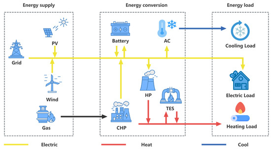
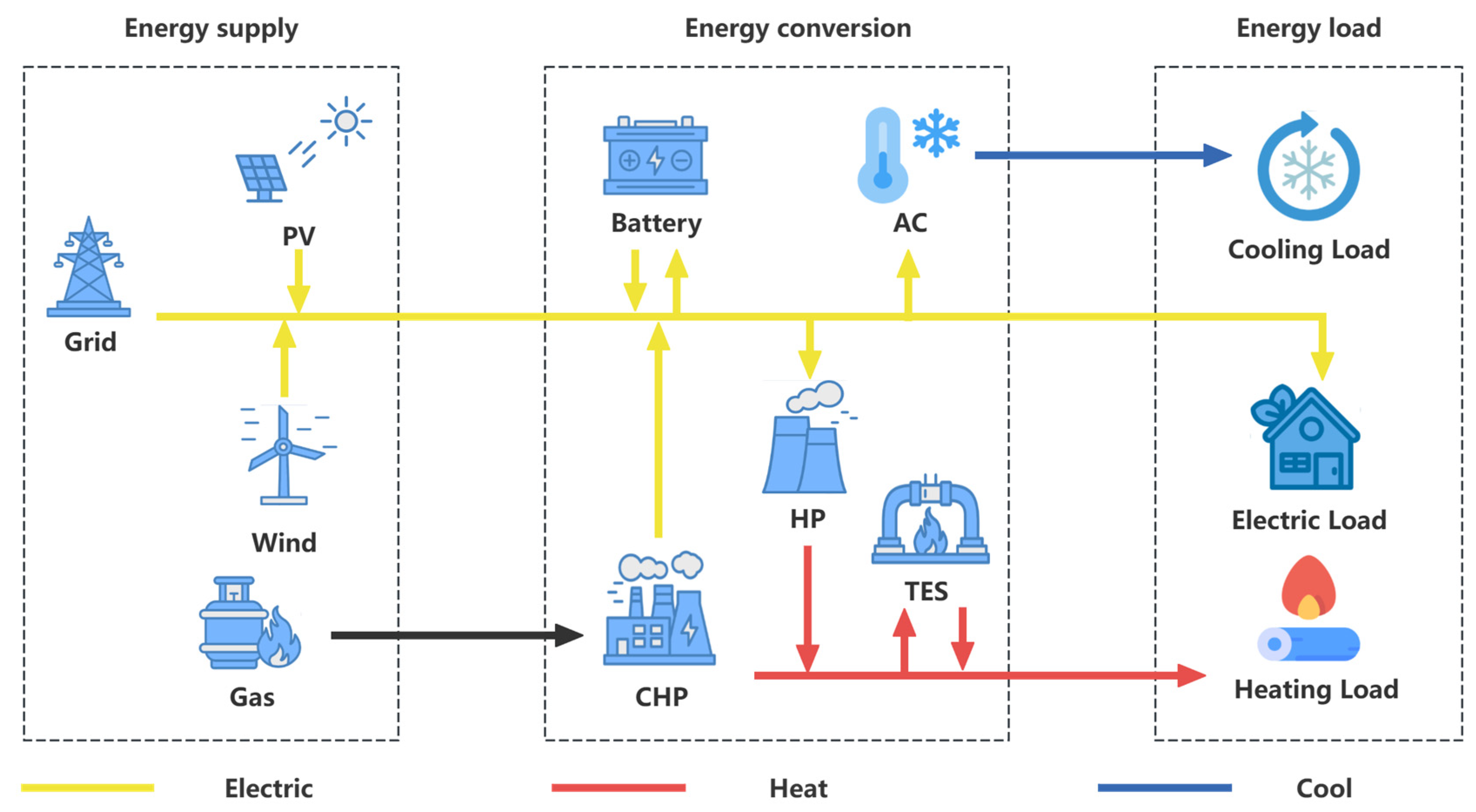
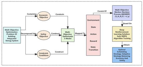
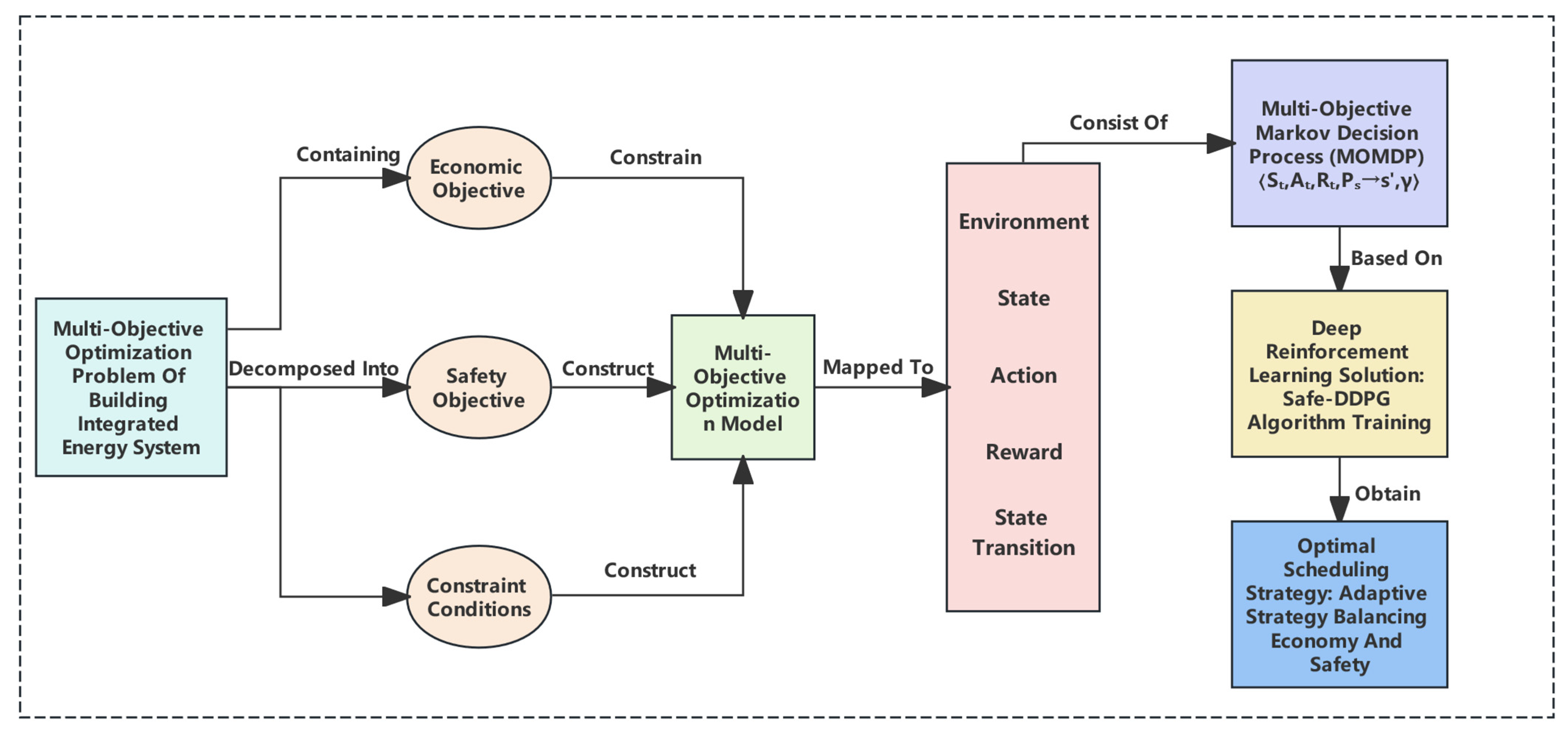
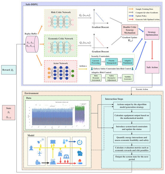
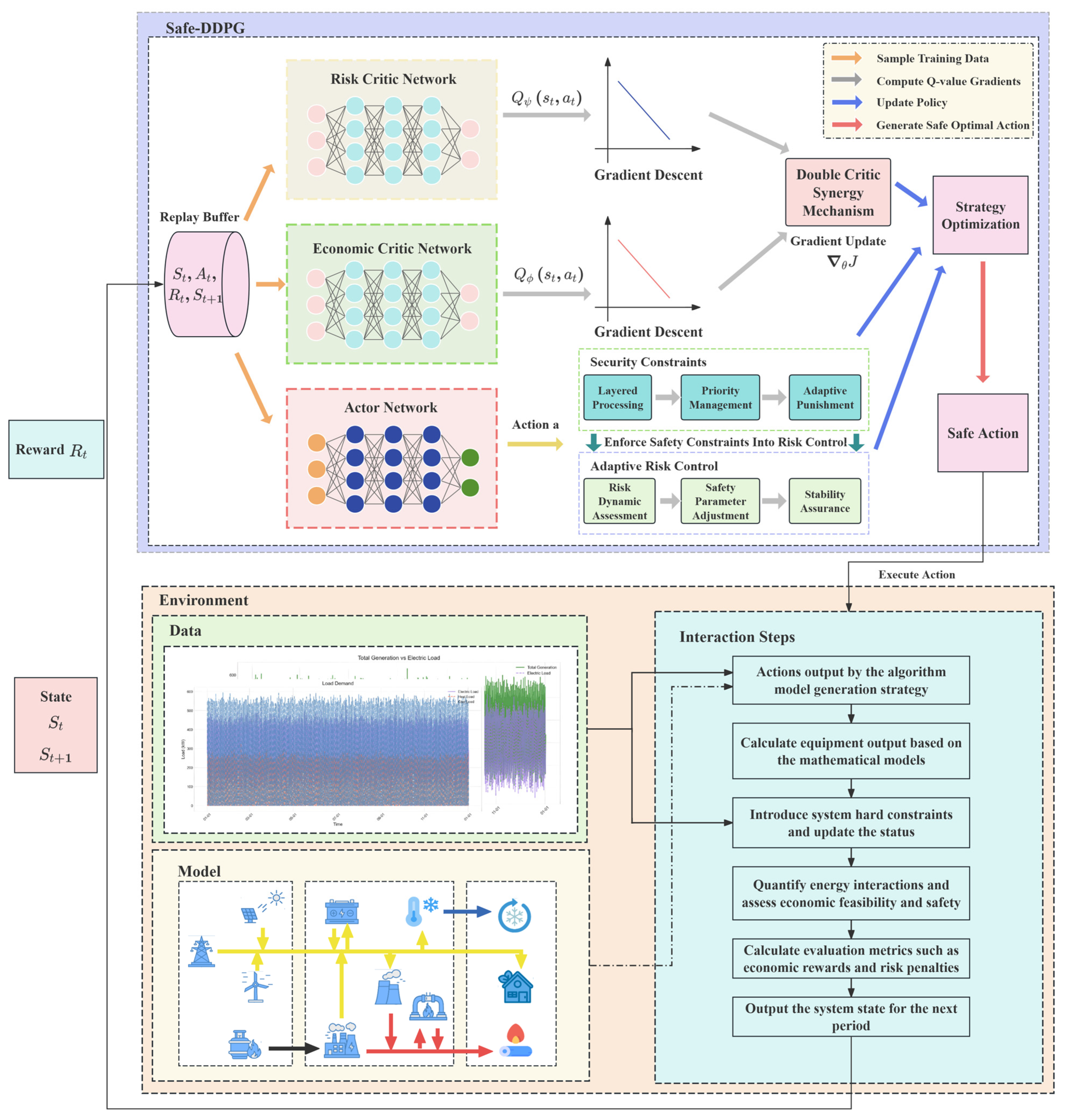
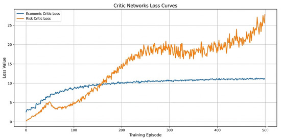
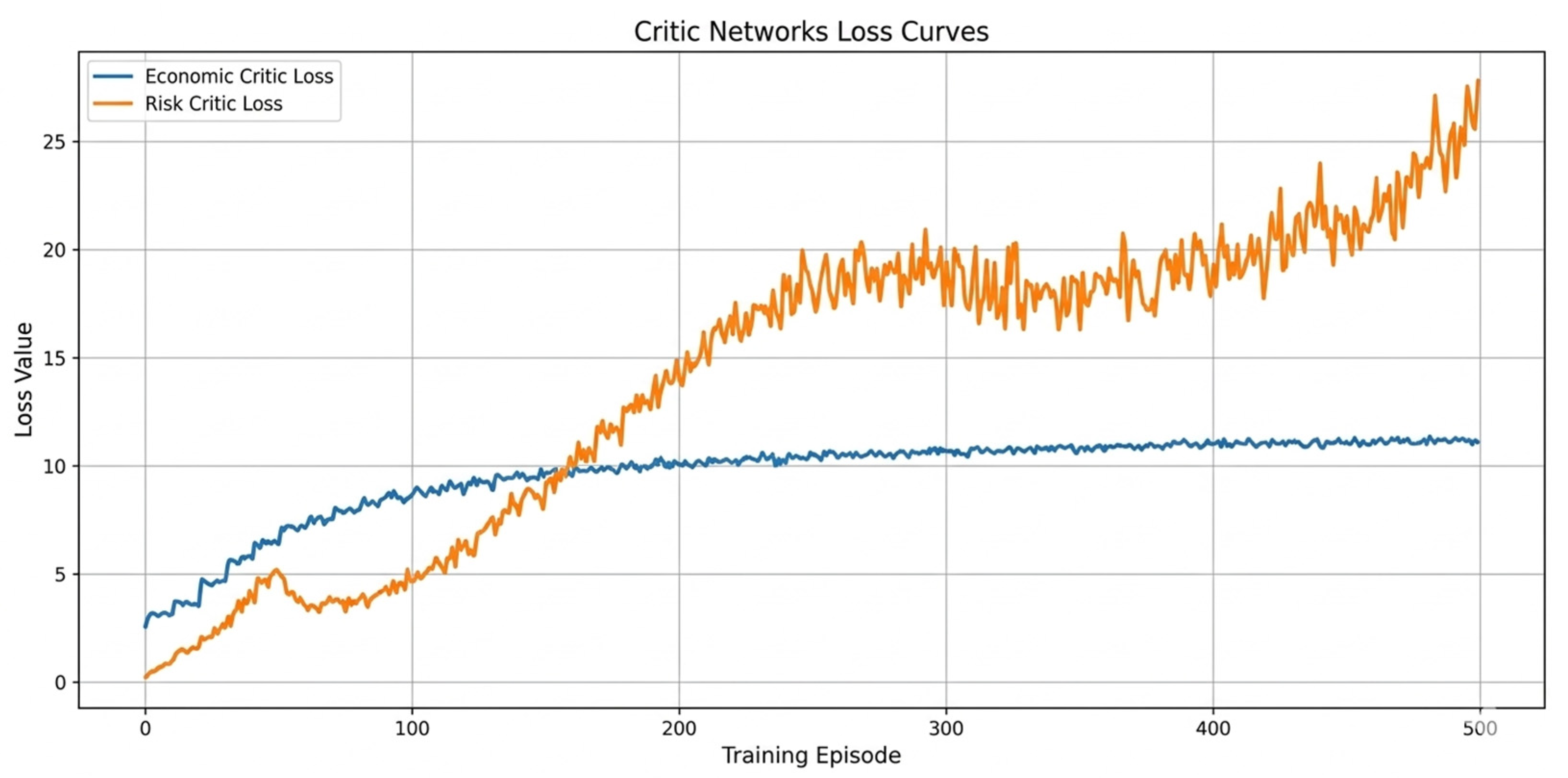
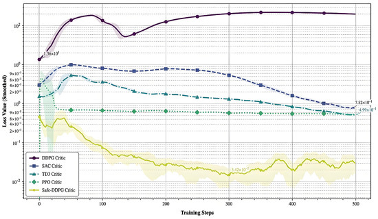
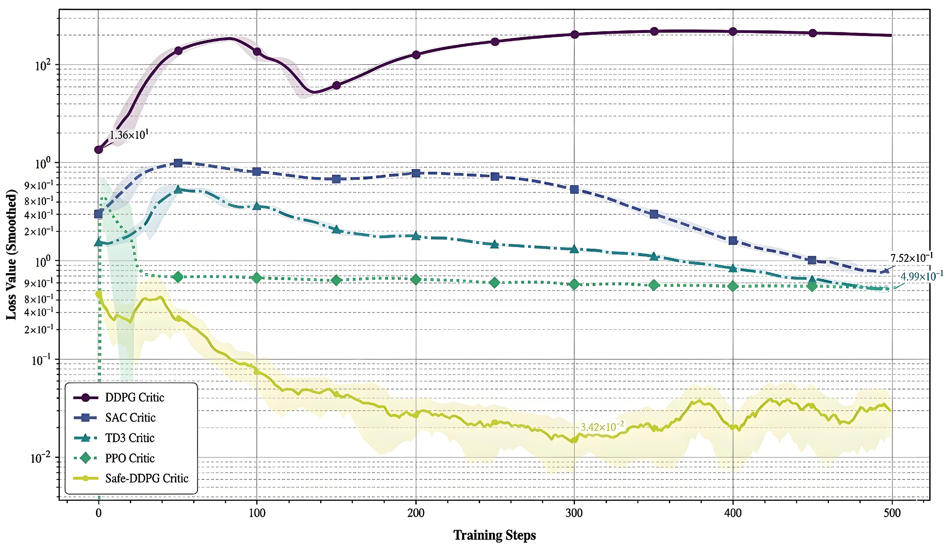
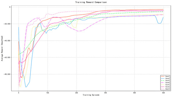
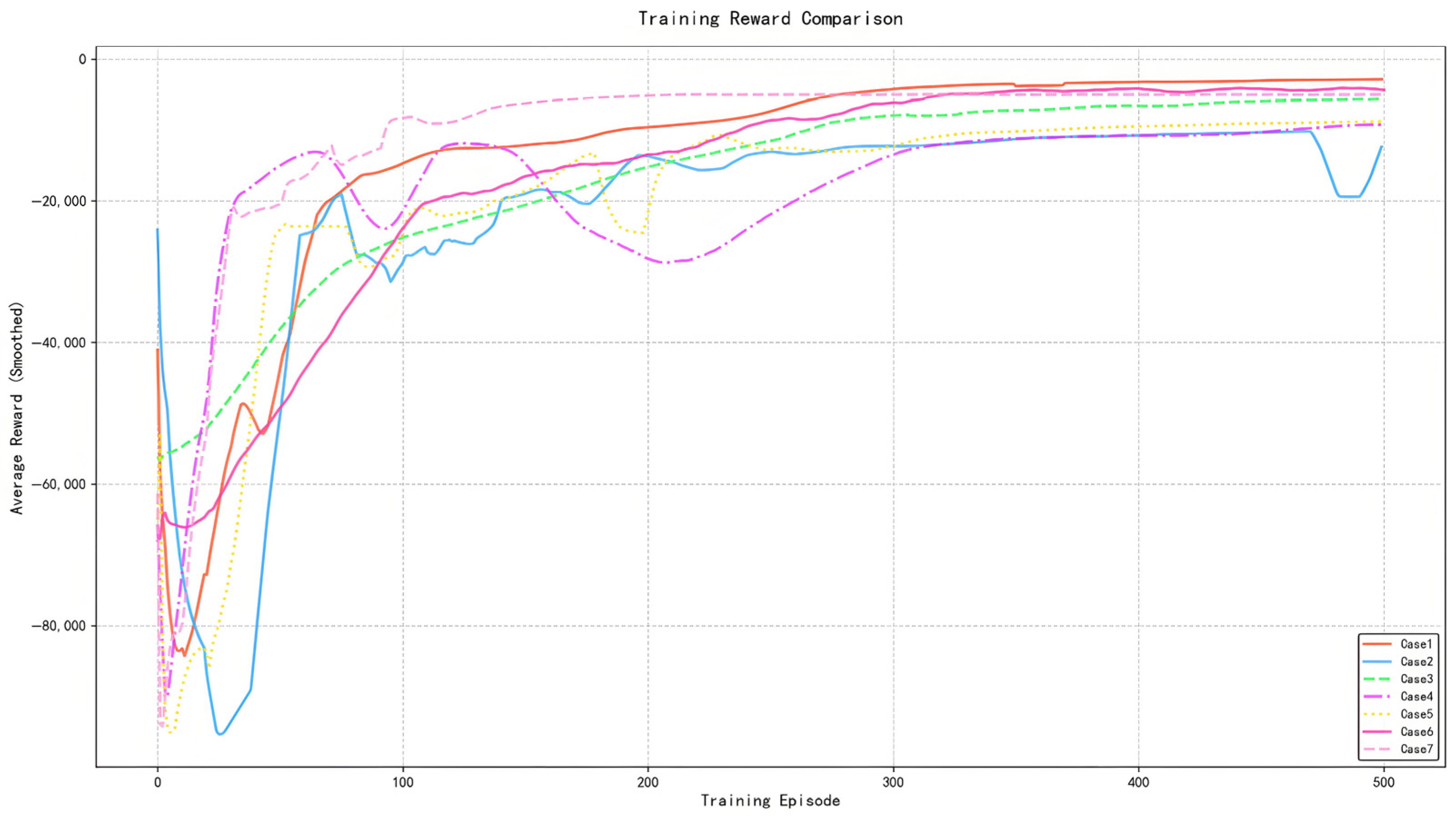
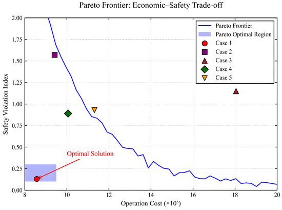
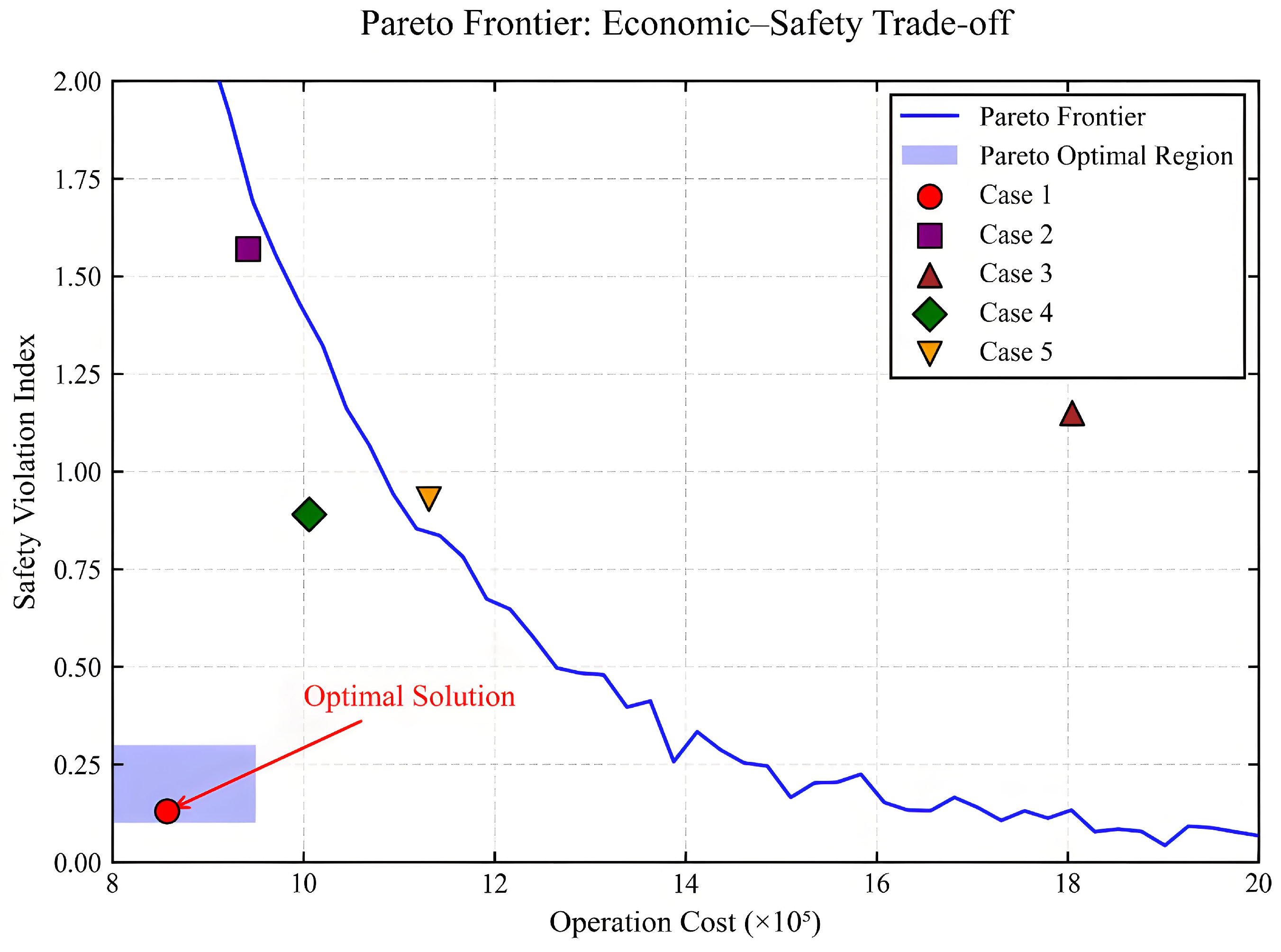
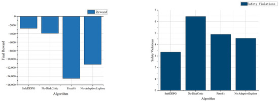
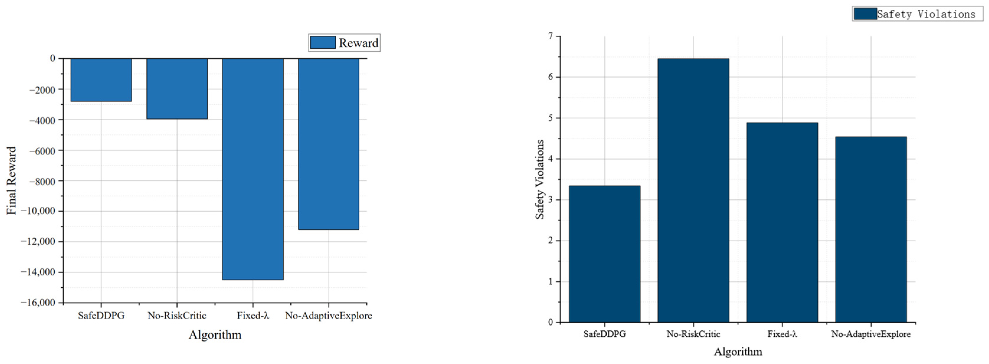

Disclaimer/Publisher’s Note: The statements, opinions and data contained in all publications are solely those of the individual author(s) and contributor(s) and not of MDPI and/or the editor(s). MDPI and/or the editor(s) disclaim responsibility for any injury to people or property resulting from any ideas, methods, instructions or products referred to in the content. |
© 2026 by the authors. Licensee MDPI, Basel, Switzerland. This article is an open access article distributed under the terms and conditions of the Creative Commons Attribution (CC BY) license.