A Two-Stage Distributionally Robust Optimization Framework for UAV-Based Dynamic Inspection with Joint Deployment and Routing

Abstract

The growing scale and complexity of industrial infrastructure make efficient and reliable inspections a critical challenge. Inspection task demands often vary dynamically, requiring efficient and demand-responsive inspection strategies to ensure stable operation. However, existing UAV inspection approaches typically deploy UAV base stations (UAV-BSs) based on fixed inspection frequencies, which are inadequate for adapting to such dynamic demands and may reduce inspection efficiency. Moreover, these approaches often rely on historical inspection data, whose empirical distributions may deviate from the true distributions, thereby compromising solution robustness. To address these issues, this paper proposes a two-stage distributionally robust optimization (TDRO) framework for joint UAV-BS deployment and inspection routing in dynamic environments. The framework accounts for uncertainties in both inspection frequency and distributional perturbations. Uncertainty sets constructed based on probability metrics are employed to capture deviations between empirical and true distributions, forming the foundation of the two-stage distributionally robust optimization model. The resulting model is solved using column-and-constraint generation (C&CG) integrated with column generation (CG), yielding robust deployment decisions and an effective trade-off between total system cost and inspection efficiency. Simulation results show that the framework effectively addresses inspection frequency uncertainty, reducing the total objective by 5.50% on average, with a further 2.16% reduction when distributional perturbations are considered.

1. Introduction

Infrastructure inspection is a crucial approach for ensuring the safe and stable operation of critical infrastructure and preventing major accidents [1]. With the continuous expansion of industrial facilities and plants and the increasing requirements for safe operation and maintenance, traditional manual inspection methods are increasingly inadequate for meeting the demands of large-scale infrastructure inspections in terms of efficiency, cost, and safety [2]. In this context, unmanned aerial vehicles (UAVs), with their high mobility, flexible deployment, and operational efficiency, have gradually become an important technology for infrastructure inspection [3]. UAV-based inspection techniques have been widely applied in industrial and infrastructure inspections, demonstrating clear advantages in improving efficiency and safety [4].

In practical applications, UAV-based inspection systems typically adopt an integrated architecture consisting of UAVs, base stations, and control centers. Through preconfigured base station deployment and inspection path planning, automated inspection operations can be achieved [5]. Compared with traditional manual approaches, UAV-based inspection significantly reduces labor costs, improves the accuracy and consistency of data acquisition, and enhances the safety and intelligence of the inspection process. In infrastructure inspection tasks, UAVs equipped with advanced sensing devices, such as high-resolution cameras and various sensors, demonstrate superior operational capabilities [6]. With the widespread application of UAV-based inspection in infrastructure inspection, it has become increasingly important to develop inspection task scheduling schemes that achieve low cost and high efficiency [7].

In recent years, UAVs have been increasingly applied to industrial facility inspections, demonstrating clear advantages in efficiency and safety. Existing studies often assume fixed inspection frequencies, while in practice, inspection tasks vary dynamically, and historical data may not fully reflect future patterns. To address these challenges, this study proposes a two-stage distributionally robust optimization (TDRO) framework for UAV-BS deployment and inspection route planning, which accounts for both task-level uncertainty and potential distributional perturbations. Figure 1 illustrates the overall solution process of the proposed framework.

Figure 1. Simplified flowchart of the proposed solution.

The main contributions of this study are summarized as follows:

(1) Unlike existing studies that typically assume deterministic inspection frequencies, we explicitly model the uncertainty of inspection tasks by constructing a multi-scenario task set derived from historical data. This set captures both scenario-specific inspection frequencies and the associated occurrence probabilities, enabling a more realistic, task-level representation of inspection requirements. Compared with classical UAV route optimization and Location-Routing Problem models, our approach prevents resource over-allocation in low-probability scenarios and provides a framework that jointly accounts for dynamic task demands and probabilistic variations, thereby enhancing the robustness and efficiency of UAV inspection planning.

(2) In contrast to conventional stochastic optimization approaches, which often neglect perturbations in the probability distributions of historical data, we construct a probability-metric-based uncertainty set that accounts for both the uncertainty in inspection frequencies and the ambiguity arising from distributional shifts. Building on this set, we develop a TDRO model that enhances decision robustness against such distributional variations, thereby improving operational efficiency under uncertain environments.

The remainder of this paper is organized as follows: Section 2 reviews the relevant literature. Section 3 introduces the research problem and formulates the mathematical model. Section 4 provides a detailed description of the algorithm for solving the TDRO model. Section 5 presents the numerical results and analysis. Finally, Section 6 concludes the paper and briefly discusses directions for future research.

2. Literature Review

This scheme originates from UAV inspections in the industrial domain, and its model is essentially a Location-Routing Problem (LRP). Therefore, this section provides a brief review of the literature on UAV inspections and applications of the LRP.

The LRP is a classic issue in the field of logistics, with its core lying in determining the location of facilities and planning transportation routes from the facilities to given nodes. It is usually divided into two stages: the first stage is the facility location decision, and the second stage is the vehicle routing planning decision. This section briefly reviews the application and solution methods of LRP in different scenarios. Reference [8] proposed a two-stage robust drone facility location problem for post-disaster humanitarian rescue, aiming to minimize the total cost in the worst-case scenario under demand uncertainty. Reference [9] constructed a robust reverse logistics network model integrating facility location and routing planning in the problem of shared bicycle recycling, and solved it using two-stage robust optimization and C&CG algorithms. Reference [10] proposed a sustainable LRP model for supply chain optimization under the background of the COVID-19 pandemic, aiming to minimize the total cost and meet operational constraints, and solved it using a genetic simulated annealing hybrid algorithm. Reference [11] established a mixed-integer LRP model with time windows for medical waste disposal, and handled uncertainty by combining chance-constrained programming and branch pricing algorithms. The two-stage location–routing framework and solution approaches adopted in these studies provide valuable modeling and methodological references for UAV-BS facility location and deployment, as well as inspection route optimization in UAV inspection operations.

In recent years, with the rapid advancement of UAV technology, UAV inspections have been increasingly adopted across various industrial sectors, enabling facility monitoring and preventive maintenance through diverse onboard equipment and integrated sensing technologies [12]. Reference [13] reviews intelligent transmission line inspection technologies based on UAVs, focusing on path planning, trajectory tracking, and fault detection. Reference [14] discusses the application of UAVs in oil and gas facility inspections, highlighting their advantages in enhancing safety and reducing operational costs. Reference [15] proposes an optimization deployment framework for UAV-based offshore wind farm inspections. Reference [7] develops a two-stage heuristic algorithm to improve trajectory quality and coverage in large-scale industrial inspection scenarios.

Alongside these application-oriented studies, a growing body of research has focused on UAV-BS deployment and inspection path optimization. Reference [16] developed an optimization model for UAV-BS inspections in large-scale facilities, incorporating energy constraints and balancing UAV-BS deployment costs with inspection path costs to minimize the overall expenditure. Reference [17] addressed UAV-BS inspections of oil and gas pipelines, proposing a two-stage optimization method aimed at minimizing the total length of inspection paths. In the first stage, the pipeline network is divided into multiple inspection segments based on UAV inspection characteristics, significantly reducing the complexity of path planning. In the second stage, an adaptive hybrid genetic–simulated annealing algorithm is applied to optimize the inspection paths. Reference [18] developed a mathematical model considering UAV power constraints and inspection time windows, aiming to address offshore oilfield inspection tasks, and proposed an improved differential evolution algorithm for its solution.

Meanwhile, some studies have also considered the impact of uncertainties arising from environmental factors. Reference [19] investigated the Vessel–UAV cooperative inspection problem for offshore oil and gas pipelines, considering the uncertainty in inspection times for each facility. A two-stage planning model with fuzzy parameters was proposed, which was solved using a hybrid genetic–tabu search algorithm. Reference [20] focused on UAV swarms in power systems and proposed a scheduling method that integrates path planning with laser-based long-range charging. By employing distributed robust optimization to address spatiotemporal and weather uncertainties, the approach achieved higher task completion rates and improved energy efficiency.

Although UAV inspections have been widely studied, several research gaps remain. Most existing studies focus on UAV-BS deployment and inspection path planning under the assumption of fixed inspection frequencies [20], without adequately considering the dynamic variations of inspection tasks within an inspection cycle. In practice, inspection frequencies vary due to equipment conditions, operational progress, and environmental factors, introducing significant task-level uncertainty [21]. Moreover, the empirical probability distribution derived from historical inspection data may deviate from the true distribution due to incomplete data, sampling bias, or potential shifts in future inspection patterns, resulting in distributional perturbations that further challenge the robustness of UAV-BS deployment strategies [22]. To address these issues, this study proposes a TDRO model that accounts for both dynamic changes in inspection frequencies and distributional perturbations in historical data, aiming to jointly optimize UAV-BS deployment and inspection route planning. In solving the model, multi-scenario inspection task sets are constructed based on historical inspection data, and a probability-metric-based uncertainty set is introduced to characterize task-level uncertainty. Subsequently, a solution approach combining the C&CG and CG algorithms is employed to ensure robust UAV-BS deployment strategies and efficient inspection route scheduling under uncertain environments.

3. System Model

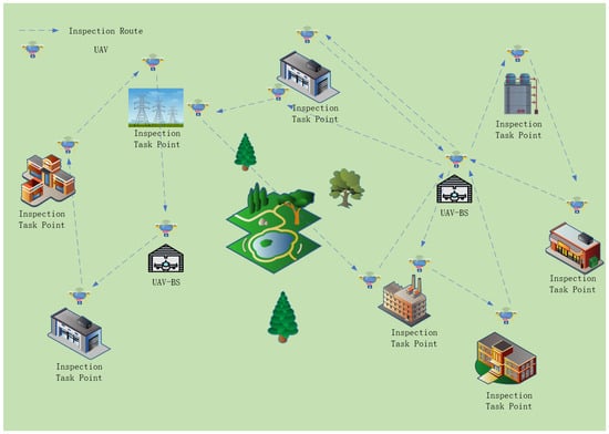
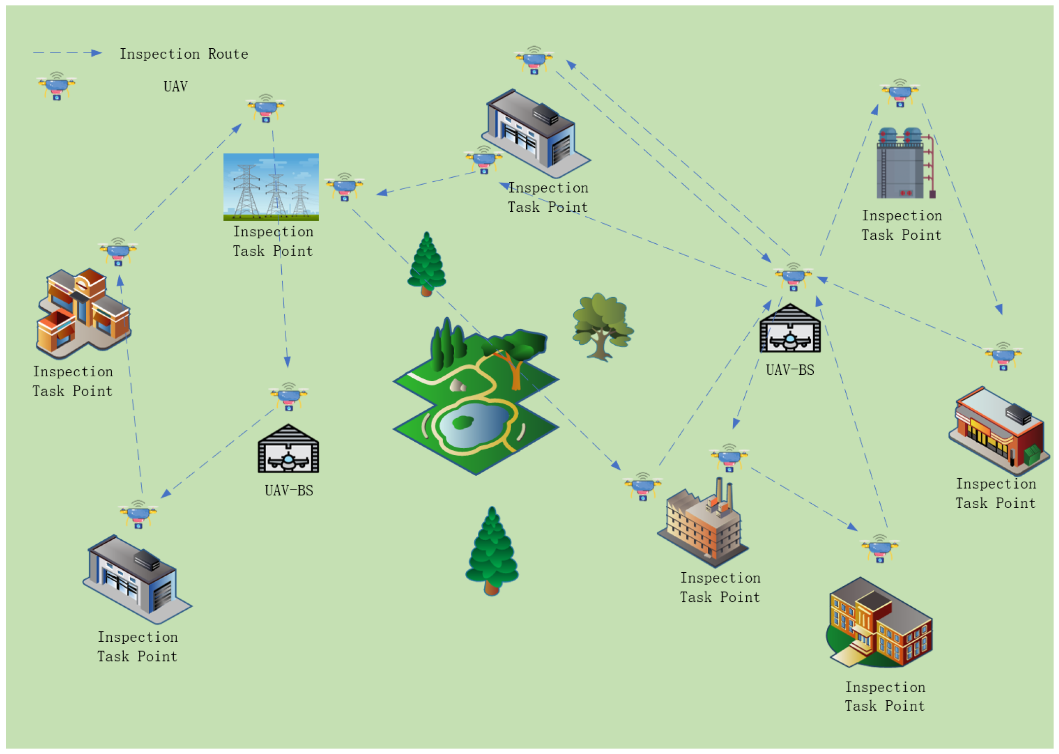
As shown in Figure 2, UAVs depart from the deployed UAV-BS, perform inspections at multiple task points, and return to their originating UAV-BS. During the inspection process, the demands of individual inspection targets vary, and their inspection frequencies dynamically change according to the actual operational conditions. Therefore, when planning UAV-BSs deployment, it is necessary to comprehensively consider both the locations of inspection task points and the dynamic inspection frequencies to satisfy the requirements of all inspection targets, achieve a rational allocation of resources, and complete inspection tasks efficiently and reliably, thereby enhancing overall system operational efficiency and inspection quality.

Figure 2. System model diagram.

In the large-scale facility inspection problem, an undirected graph $G=(V,E)$ is considered, where the node set V includes the candidate UAV-BS deployment location D and the inspection task point C, and the arc set E represents connections between any two nodes. The dynamic inspection frequencies of the inspection tasks constitute the main source of uncertainty that the model needs to address. To characterize this uncertainty, S scenarios are generated based on historical inspection data, from which the corresponding empirical probability distribution $P_v^0$ is obtained. Furthermore, to address the perturbations in the historical task probability distribution, two types of confidence sets based on the $L_1$ norm and $L_{\infty }$ norm are adopted to construct a distributionally robust uncertainty set for the inspection tasks [23]. Specifically, the $L_1$ norm tolerance ${\epsilon }_1$ is used to limit the cumulative deviation of all worst-case probability distribution scenarios from the empirical distribution, thereby controlling the overall probability fluctuations, while the $L_{\infty }$ norm tolerance ${\epsilon }_{\infty }$ constrains the maximum deviation of any individual scenario probability, thus limiting extreme deviations of individual scenario probabilities. By combining these two types of norm-based constraints, the model can simultaneously control the fluctuations of historical scenario probabilities from both the total deviation and extreme deviation perspectives, resulting in the following form of the uncertainty set $\omega$:

$$\omega =\left[\begin{array}{c}0\le p_v\le 1,\forall v\in S\hfill \\ {\displaystyle \sum _{v\in S}}{p}_v=1\hfill \\ {\displaystyle \sum _{v\in S}}\left|p_v-p_v^0\right|\le {\epsilon }_1\hfill \\ \underset{1\le v\le S}{max}\left|p_v-p_v^0\right|\le {\epsilon }_{\infty }\hfill \end{array}\right]$$

(1)

3.1. Arc-Based Graph Model

To highlight the focus of this study on the modeling and optimization of dynamic inspection tasks, a reasonable abstraction of the UAV inspection process is adopted during the modeling stage. Specifically, the dynamic variations of energy consumption during flight and inspection are not explicitly modeled; instead, flight distance constraints are adopted as a proxy for energy limitations. Moreover, other practical operational factors, such as weather conditions and UAV communication limitations, are beyond the scope of the current model. In addition, it is assumed that there are no no-fly zones within the inspection area and that any two nodes can be connected via pre-planned flight paths, which are represented by the arc set E in the graph.

An inspection task is considered completed once the corresponding inspection task point is visited. These assumptions are intended to emphasize the impact of inspection frequency uncertainty and distributional perturbations on UAV-BS deployment and task scheduling decisions. The relevant symbols and parameter definitions are summarized in Table 1. Given all candidate UAV-BS deployment locations and inspection task points, the arc-based graph model (AGM) can be formulated as follows:

Table 1. Notation Definition.

Sets
D	Set of candidate UAV-BS deployment locations
C	Set of inspection task points
V	Set of candidate UAV-BS deployment locations and inspection task points
K	Set of UAV inspection tasks
S	Set of historical inspection data
E	Set of arcs connecting any pair of nodes
Parameters
$f_i$	Deployment cost of establishing a UAV-BS at candidate location $i\in D$
$\rho$	Weight coefficient balancing deployment cost and inspection efficiency
s	UAV flight speed
$d_{ij}$	Distance between node i and node j, where $(i,j)\in E$
$h_j$	Flight distance consumed at inspection task point $j\in C$
$L_{max}$	Maximum flight distance of the UAV
$z_j$	Additional number of inspections required for task point $j\in C$ based on historical data
N	Number of elements in set V
Decision Variables
$y_i$	Binary variable indicating whether a UAV-BS is deployed at candidate location $i\in D$ (1 if deployed, 0 otherwise)
$p_{ik}$	Binary variable indicating whether inspection task $k\in K$ is assigned to UAV-BS $i\in D$ (1 if assigned, 0 otherwise)
$x_{ijk}$	Binary variable indicating whether arc $(i,j)\in E$ is traversed in inspection task $k\in K$ (1 if selected, 0 otherwise)
$u_{ik}$	Auxiliary variable for subtour elimination

First-stage decision:

$$\underset{y,p}{min}\left(\sum _{i\in D}{f}_i{y}_i+\rho \underset{F\in \omega }{max}{E}_F\left(Q_{f\left(y,p,z^{*}\right)\in F\left(y,p,z^{*}\right)}\right)\right)$$

(2)

s.t.

$$p_{ik}\le y_i\forall i\in D,\forall k\in K$$

(3)

$$y_i,p_{ik}\in \{0,1\}\forall i\in D,\forall k\in K$$

(4)

Two-stage decision:

$$Q(y,p,z^{*})=\underset{f(y,p,z^{*})}{min}\sum _{i\in D\cup C}\sum _{j\in D\cup C}\sum _{k\in K}{x}_{ijk}{d}_{ij}/s$$

(5)

s.t.

$$\sum _{j\in C}{x}_{ijk}\le p_{ik}\forall i\in D,\forall k\in K$$

(6)

$$\sum _{i\in D\cup C}\sum _{k\in K}{x}_{ijk}=1+z_j\forall j\in C$$

(7)

$$\sum _{i\in D\cup C}\sum _{j\in D\cup C}{x}_{ijk}{d}_{ij}+\sum _{j\in C}{h}_j\sum _{i\in D\cup C}\sum _{j\in C}{x}_{ijk}\le L_{max}\forall k\in K$$

(8)

$$\sum _{i\in D}\sum _{j\in D\cup C}{x}_{ijk}\le 1\forall k\in K$$

(9)

$$\sum _{i\in D\cup C}{x}_{ijk}-\sum _{r\in D\cup C}{x}_{jrk}=0\forall j\in C,\forall k\in K$$

(10)

$$\sum _{j\in C}{x}_{jik}-1\ge (p_{ik}-1)M\forall i\in D,\forall k\in K$$

(11)

$$u_{ik}-u_{jk}+N{x}_{ijk}\le N-1\forall i,j\in C,\forall k\in K,i\ne j$$

(12)

$$x_{iik}=0\forall i\in D\cup C,\forall k\in K$$

(13)

$$u_{jk}\in \{0,1\}\forall j\in D\cup C,\forall k\in K$$

(14)

$$x_{ijk}\in \{0,1\}\forall i,j\in D\cup C,\forall k\in K$$

(15)

In the first stage, F denotes the probability measure of the probability distribution $f(y,p,z)$, and the notation $E_F[.]$ represents the expectation under the probability distribution defined by F. The objective function (2) represents the integrated trade-off value, which is composed of the first-stage UAV-BS deployment cost and the weighted expected inspection time in the second stage. Constraint (3) ensures that an inspection task k can be assigned to a candidate UAV-BS i only if the UAV-BS is deployed, while constraint (4) specifies the feasible values of the first-stage decision variables.

In the second stage, the objective function (5) represents the total inspection time. Constraint (6) ensures that the corresponding inspection routes can be activated only if inspection task k is assigned. Constraint (7) ensures that the required number of inspections for each task point is satisfied across all scenarios. Constraint (8) ensures that, for each inspection task k, the total distance during the inspection process, including the distance consumed at inspection task points, does not exceed the UAV’s maximum flight distance. Constraint (9) ensures that each inspection task k is executed at most once. Constraint (10) enforces the flow conservation of the inspection routes. Constraint (11) requires UAVs to return to their original departure UAV-BSs after completing all assigned tasks. Constraint (12) eliminates subtours in the inspection routes to ensure route continuity. Constraint (13) prohibits inspection task points from visiting themselves. Constraints (14) and (15) specify the feasible values of the second-stage decision variables.

3.2. Path-Based Set Partitioning Model

Although the aforementioned AGM can effectively solve the UAV-BS deployment and task scheduling problem under dynamic inspection environments, its computational complexity increases rapidly in large-scale settings. To improve computational efficiency, the Dantzig–Wolfe decomposition approach is introduced to reformulate the AGM, leading to a path-based set partitioning model (PSPM). This model transforms the arc-based decisions in the AGM into the selection of complete inspection routes, thereby effectively reducing the size of the solution space [9]. Specifically, feasible solutions composed of arc variables in the AGM can be mapped to a set of complete inspection routes that satisfy flow conservation and task coverage constraints, while the path variables in the PSPM correspond to feasible combinations of these arc variables. By extending the decision structure from local arcs to complete routes, the PSPM structurally reduces the dimensionality of decision variables and provides a solid modeling foundation for efficiently solving large-scale problems.

To facilitate the transformation of the model, three key variables, denoted as $x_r$, $a_{rj}$, and $b_{ri}$, are introduced. Variable $x_r$ indicates whether an inspection route $r\in R$ is selected, where R denotes the set of all feasible inspection routes; $x_r=1$ if route r is selected, and 0 otherwise. Variable $a_{rj}$ equals 1 if inspection route r covers inspection task point j, and 0 otherwise. Variable $b_{ri}$ equals 1 if inspection route r originates from UAV-BS i, and 0 otherwise. With the introduction of these variables, the arc selection problem in the AGM can be transformed into a route selection problem, thereby reducing the dimensionality of the model and improving computational efficiency.

Through the conversion of the above variables, the PSPM of TDRO can be expressed as:

$$\underset{x,y}{min}\left(\sum _{i\in D}{f}_i{y}_i+\underset{F\in \omega }{max}{E}_F\left(Q_{f(y,z^{*})\in F(y,z^{*})}\right)\right)$$

(16)

s.t.

$$y_i\in \{0,1\}\forall i\in D$$

(17)

$$Q(y,p,z^{*})=\underset{f(y,z^{*})}{min}{c}_r{x}_r$$

(18)

s.t.

$$\sum _{r\in R}{a}_{rj}{x}_r=1+z_j\forall j\in C$$

(19)

$$b_{ri}{x}_r\le y_i\forall i\in D,\forall r\in R$$

(20)

$$x_r\in \{0,1\}\forall r\in R$$

(21)

Here, $c_r$ denotes the weighted value of the inspection time associated with route r. Equations (16) and (18) represent the first-stage and second-stage objective functions of the PSPM, respectively, and their interpretations are consistent with those in the AGM. Constraints (17) and (21) define the domains of the decision variables. Constraint (19) corresponds to constraint (7) in the AGM and ensures that the demand of each inspection task point is satisfied. Constraint (20) corresponds to constraints (3) and (6) in the AGM, specifying that an inspection route can be selected only if the corresponding UAV-BS is deployed. Furthermore, constraints (8)–(13) in the AGM, which ensure the feasibility of inspection routes, are not explicitly included in the PSPM. Instead, they are implicitly enforced during the route generation process and embedded in the construction of the feasible inspection route set.

Given that the outer-stage $max$ problem in the second stage consists of S mutually independent inspection scenarios and that there are no coupling constraints among decision variables across scenarios, the problem can be further reformulated as a discrete-scenario-based model (D-PSPM) to facilitate solutions and clarify the model structure. The D-PSPM can be expressed as follows:

$$\underset{y}{min}\sum _{i\in D}{f}_i{y}_i+\underset{p\in \omega }{max}\underset{x}{min}\sum _{v\in S}\sum _{r\in R}{p}_v{c}_r{x}_r^v$$

(22)

s.t.

$$\sum _{r\in R}{a}_{rj}{x}_r^v=1+z_j^v\forall j\in C,\forall v\in S$$

(23)

$$b_{ri}{x}_r^v\le y_i\forall i\in D,\forall r\in R,\forall v\in S$$

(24)

$$y_i,x_r^v\in \{0,1\}\forall i\in D,\forall r\in R,\forall v\in S$$

(25)

Here, $p_v$ denotes the probability of scenario v occurring, and $x_r^v$ represents the selection of inspection route r under scenario v. The model aims to determine the optimal UAV-BS deployment in the first stage, ensuring that, even under perturbations in the probability distribution, the inspection demands of each scenario in the second stage can still be satisfied through optimal route adjustments based on this deployment, thereby achieving an optimal trade-off in the objective function.

4. Solution Method

Perturbations in the historical task probability distribution result in a max-min bi-level structure in the second stage of the D-PSPM, making the model difficult to solve directly. To address this, a solution framework based on the C&CG algorithm is developed to iteratively approach the robust optimal solution [24]. To handle the challenge of enumerating large-scale feasible route sets, a CG algorithm is further incorporated to dynamically generate feasible inspection routes and construct a solution space that covers the optimal solution. The C&CG algorithm iteratively solves the master problem and subproblems to gradually approach the robust optimal solution, while the CG algorithm updates the route set during the iterations to ensure that the generated set spans the complete solution space required to cover the global optimum. Through this coordinated mechanism, the first-stage UAV-BS deployment and the second-stage inspection task scheduling converge to the global optimal solution within a finite number of iterations.

4.1. Column-And-Constraint Generation Algorithm

The C&CG algorithm decomposes the D-PSPM problem into a master problem and a subproblem, and achieves the global optimum through iterative solution. The master problem determines the deployment scheme of UAV-BSs, while the subproblem, given a fixed deployment scheme, identifies the worst-case probability distribution and the corresponding optimal inspection scheduling. The algorithm starts by initializing a deployment scheme and passing it to the subproblem to obtain the worst-case probability distribution under this scheme. The solution of the subproblem is then fed back to the master problem to generate additional constraints, ensuring that the deployment scheme obtained in the next iteration can effectively hedge against the worst-case probability distribution identified by the subproblem. Since the master problem considers only a subset of worst-case probability distribution scenarios in each iteration, its optimal value reflects only these scenarios. Therefore, compared with the original problem that considers all worst-case probability distributions, it can be regarded as a lower bound. On the other hand, the deployment scheme provided by the master problem is not necessarily globally optimal; thus, under this scheme, the optimal inspection scheduling obtained from the subproblem serves as an upper bound of the original problem.

Through iterative procedures, the master problem successively introduces new constraints to refine the UAV-BS deployment, allowing the deployment solution to gradually approach the global optimum. Meanwhile, the gap between the upper and lower bounds of the master and subproblems is progressively reduced until convergence is achieved within a finite number of iterations, resulting in the globally optimal UAV-BS deployment and inspection task scheduling. The master problem in the C&CG algorithm can be formulated as follows:

$$\underset{y,x}{min}{f}_i{y}_i+\eta$$

(26)

s.t.

$$\eta \ge \sum _{v\in S}\sum _{r\in R}{p}_v^{*}{c}_r{x}_r^{v,l}l=1,2,3,...,t$$

(27)

$$\sum _{r\in R}{a}_{rj}{x}_r^{v,l}=1+z_j^v\forall j\in C,\forall v\in S,l=1,2,3,...,t$$

(28)

$$b_{ri}{x}_r^{v,l}\le y_i\forall i\in D,r\in R,\forall v\in S,l=1,2,3,...,t$$

(29)

$$y_i,x_r^{v,l}\in \{0,1\}\forall i\in D,r\in R,\forall v\in S,l=1,2,3,...,t$$

(30)

Here, $l=1,2.3...,t$ represents the worst probability distribution that is continuously added to the main problem.

By discretizing the sample space, S mutually independent inspection task scenarios can be obtained. Under the UAV-BS deployment provided by the master problem, the second-stage problem of the D-PSPM for each inspection scenario can be solved using the CG algorithm to obtain the corresponding optimal inspection scheduling $x_r^{v,*}$. Based on this, the subproblem in the C&CG algorithm can be formulated as follows:

$$\underset{p}{max}\sum _{v\in S}\sum _{r\in R}{p}_v{c}_r{x}_r^{v,*}$$

(31)

s.t.

$$\sum _{v\in S}\left|p_v-p_0^v\right|\le {\epsilon }_1$$

(32)

$$\underset{1\le v\le S}{max}\left|p_v-p_0^v\right|\le {\epsilon }_{\infty }$$

(33)

$$\sum _{v\in S}{p}_v=1$$

(34)

$$0\le p_v\le 1\forall v\in S$$

(35)

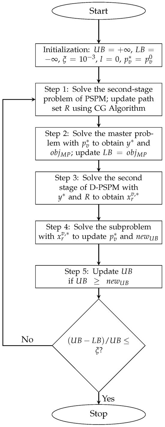
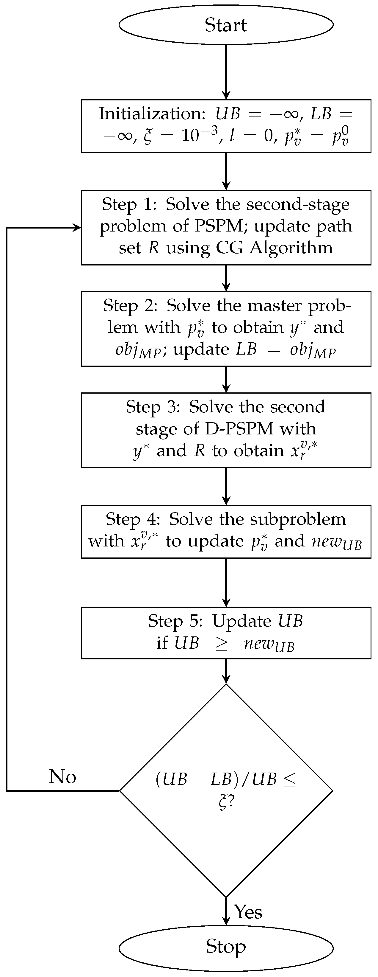
Here, ${\epsilon }_1$ and ${\epsilon }_{\infty }$ denote the tolerance values for the $L_1$ and $L_{\infty }$ norms, respectively, which constrain the cumulative total deviation between the true distributions and the empirical distribution across all scenarios, as well as the maximum deviation of the true distribution from the empirical distribution for any individual scenario. This subproblem can be solved directly using a solver. The algorithm iteratively improves the UAV-BS deployment by alternately solving the master and subproblems, converging to the global optimum within a finite number of iterations. The proposed algorithm is illustrated in the following flowchart:

The algorithm takes the initial path set R and historical inspection probability distribution $p_v^0$ as inputs. It initializes $UB$, $LB$, $\xi$, l, and $p_v^{*}$, then iteratively solves the second-stage problem of PSPM to update the path set, solves the master problem to update the deployment scheme and lower bound, and solves the subproblem to update the worst-case distribution and upper bound. Convergence is achieved when $(UB-LB)/UB\le \xi$; otherwise, the worst-case distribution is added to the master problem and the iteration continues. The outputs are the optimal deployment scheme $y^{*}$, the worst-case distribution $p_v^{*}$, and the optimal inspection scheduling $x_r^{v,*}$ for each scenario. The flowchart is shown in Figure 3.

Figure 3. C&CG Algorithm Solution Flowchart.

4.2. Column Generation Algorithm

To more efficiently construct the feasible route set, the CG algorithm is adopted. The core idea of CG is to iteratively generate new columns, i.e., inspection routes, rather than constructing all routes at once, thereby significantly reducing the computational complexity of the model. Based on a given initial route set, solving the relaxed master problem yields the optimal inspection solution under the current route set; however, this solution does not account for all possible inspection routes and may therefore not be globally optimal. The dual values of the relaxed master problem provide critical information for the subproblem, which iteratively adds new routes to the route set that could potentially further reduce the total cost. When the subproblem can no longer generate new cost-reducing routes, it indicates that the route set has covered all critical routes required to construct the global optimal solution, thereby guaranteeing the global optimality of the final solution.

Due to the particular structure of the problem studied in this paper, the conventional CG algorithm cannot be directly applied to the LRP. Therefore, an auxiliary model is constructed to assist in generating routes that can potentially reduce the total cost. The auxiliary model is as follows:

$$\underset{x}{min}\sum _{v\in S}\sum _{r\in R}{p}_v{c}_r^{*}{x}_r^v$$

(36)

s.t.

$$\sum _{r\in R}{a}_{rj}{x}_r^v=1+z_j\forall j\in C,\forall v\in S$$

(37)

$$0\le x_r^v\le 1\forall r\in R,\forall v\in S$$

(38)

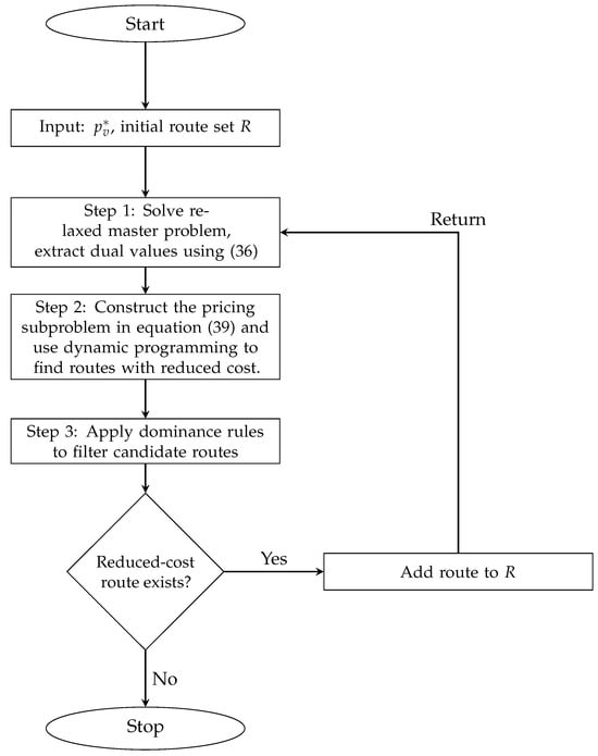
The auxiliary model corresponds to the relaxed master problem in the CG algorithm, where the total cost of a route $c_r^{*}$ includes the weighted value of the inspection time and the deployment cost of the UAV-BS from which the route departs. Reference [25] has proven that new reduced cost routes generated based on this relaxed master problem can cover all potentially reduced cost routes in the original problem, thereby guaranteeing the optimality of the solution. By solving the relaxed master problem, the dual variable values ${\alpha }_{jv}$ corresponding to constraints (37) can be obtained. These dual variables are used in the CG subproblem to evaluate whether a newly generated route has the potential to reduce the total cost. If a new route exhibits a negative reduced cost after considering the above dual information, it indicates that the route may lead to a better solution and should be added to the route set. The reduced cost for each newly generated route can be calculated as follows:

$${\widehat{c}}_r=f_i+\sum _{j\in C}{\alpha }_{jv}+\sum _{(i,j)\in E}{c}_{ij}$$

(39)

The subproblem of the CG algorithm can essentially be formulated as a shortest path problem. Given the large problem scale and the vast number of possible routes, a dynamic programming labeling algorithm is employed for its solution. During the solution process, the labeling algorithm is combined with dominance rules to enable efficient search. The label associated with each node is defined as $L_i=(i,C_i,D_i,V_i)$, where i denotes the current node, C represents the current reduced cost of the partial path, D denotes the accumulated travel distance of the partial path, and V indicates the set of nodes that have already been visited along the current path. When the UAV departs from the origin node i, an initial label $L_i=(i,0,0,\left[i\right])$ is assigned. When the UAV travels from node i to node j, the label can be extended to $L_j=(j,C_j,D_j,V_j)$ according to the following rules:

$$C_j=C_i+c_{ij}-{\alpha }_{jv}$$

(40)

$$D_j=D_i+d_{ij}+h_j$$

(41)

$$V_j=V_i+j$$

(42)

All unvisited nodes are examined based on the visited node set V, and label extension is performed accordingly. To avoid excessive enumeration of labels, dominance rules are introduced to filter the path set. The dominance rule is defined as follows: if $V_i\ge V_j$ and $C_j\le C_i$, then label $L_i$ is said to dominate label $L_j$, and label $L_j$ can be discarded without affecting the optimality of the final solution. The detailed procedure of the CG algorithm is summarized in Figure 4.

Figure 4. CG Algorithm Solution Flowchart.

The flowchart illustrates the proposed column generation procedure for UAV inspection. The inputs are the initial inspection route set and the current probability distribution of inspection tasks. The algorithm iteratively generates new routes with reduced cost, applies dominance rules to remove redundant paths, and updates the route set until no further improvement is possible. The output is an inspection route set that covers all critical routes necessary to obtain the global optimal solution.

5. Simulation Experiment

This section presents four experiments designed to evaluate the proposed model and solution method. For parameter settings, reference [16] is adopted to enhance the rationality of the experimental data, and key parameters such as UAV-BS deployment costs and UAV flight speeds are kept consistent with that study. In terms of modeling, the original model in [16], which uses energy and time as constraints, is transformed into a model where equivalent flight distance serves as the core constraint. Both the maximum flight distance and the distance consumption for each inspection task point are recalculated based on the original data to ensure the accuracy of the experimental design. In addition, to suit the scenarios of the current study, all historical data and probability distributions for the inspection task points are independently generated. This design maintains comparability with existing studies while ensuring the reasonableness and relevance of the experimental setup. The experiments are conducted in an 18 km × 18 km area, and all algorithms are implemented in Python 3.12.4 using Gurobi 11.0.3, running on a CPU: 13th Gen Intel(R) Core(TM) i7-13700F @ 2.10 GHz, with 32 GB RAM, under Windows 10. Detailed parameter settings are presented in Table 2.

Table 2. Experimental parameter settings.

Parameter Name	Parameter Symbol	Value
$f_i$	Deployment cost of UAV-BS	30
$L_{\max }$	Maximum flight distance of UAV (km)	39.45
$\rho$	Weight of cost and time	30
s	UAV flight speed (m/min)	900
R	Number of scenarios	10
${\epsilon }_1$	Tolerance of $L_1$-norm	0.2
${\epsilon }_{\infty }$	Tolerance of $L_{\infty }$-norm	1.0
$h_j$	Flight distance consumed at inspection node (m)	9000

5.1. Validity Experiment

To verify the effectiveness of the proposed model and solution method, an effectiveness experiment is designed in this section. The experiments use the publicly available dataset [26], which has been widely adopted in studies on the LRP. To satisfy the requirements of the inspection scenarios, the coordinate location information is obtained from a scaled version of the dataset, while the inspection task demands and probability distributions are redefined according to the specific research problem of this study.

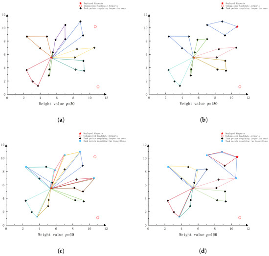
Figure 5 presents the UAV-BS deployment and task scheduling results under different weight settings and inspection frequency conditions, encompassing four scenarios in total, two weight levels (30 and 150) and two types of inspection frequency conditions (unchanged and varying), which are used to comprehensively evaluate the effectiveness of the proposed model. Each colored line represents an inspection task. When the inspection frequency remains unchanged, comparing the results under different weight levels reveals significant differences in the UAV-BS deployment schemes. Specifically, with a lower weight, the model tends to reduce the number of deployed UAV-BSs to lower the deployment cost, whereas with a higher weight, the model increases the number of UAV-BSs to shorten the inspection time. This adjustment is reflected in some inspection tasks being reassigned to more advantageous UAV-BS locations, while the remaining tasks are reorganized through path reconstruction to form new inspection routes. In both weight settings, all inspection tasks are completed, indicating that the model is feasible under different trade-off preferences.

Figure 5. UAV-BS Deployment and Inspection Task Scheduling (a) Inspection Task Scheduling under Fixed Frequency, Weight 30. (b) Inspection Task Scheduling under Fixed Frequency, Weight 150. (c) Inspection Task Scheduling under Variable Frequency, Weight 30. (d) Inspection Task Scheduling under Variable Frequency, Weight 150.

When the inspection frequency varies, comparing results under the same weight level shows that the model can adaptively adjust the scheduling scheme according to changes in task demands. Specifically, after incorporating new inspection requirements, tasks are reassigned, and paths are optimized so that inspection routes remain as short as possible while satisfying all demands, thereby ensuring that tasks can still be completed despite variations in inspection frequency. In summary, the proposed model not only generates differentiated and feasible deployment schemes under different weight settings but also maintains stable and effective task scheduling capabilities under varying inspection frequencies, demonstrating strong adaptability and robustness.

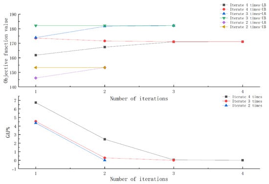
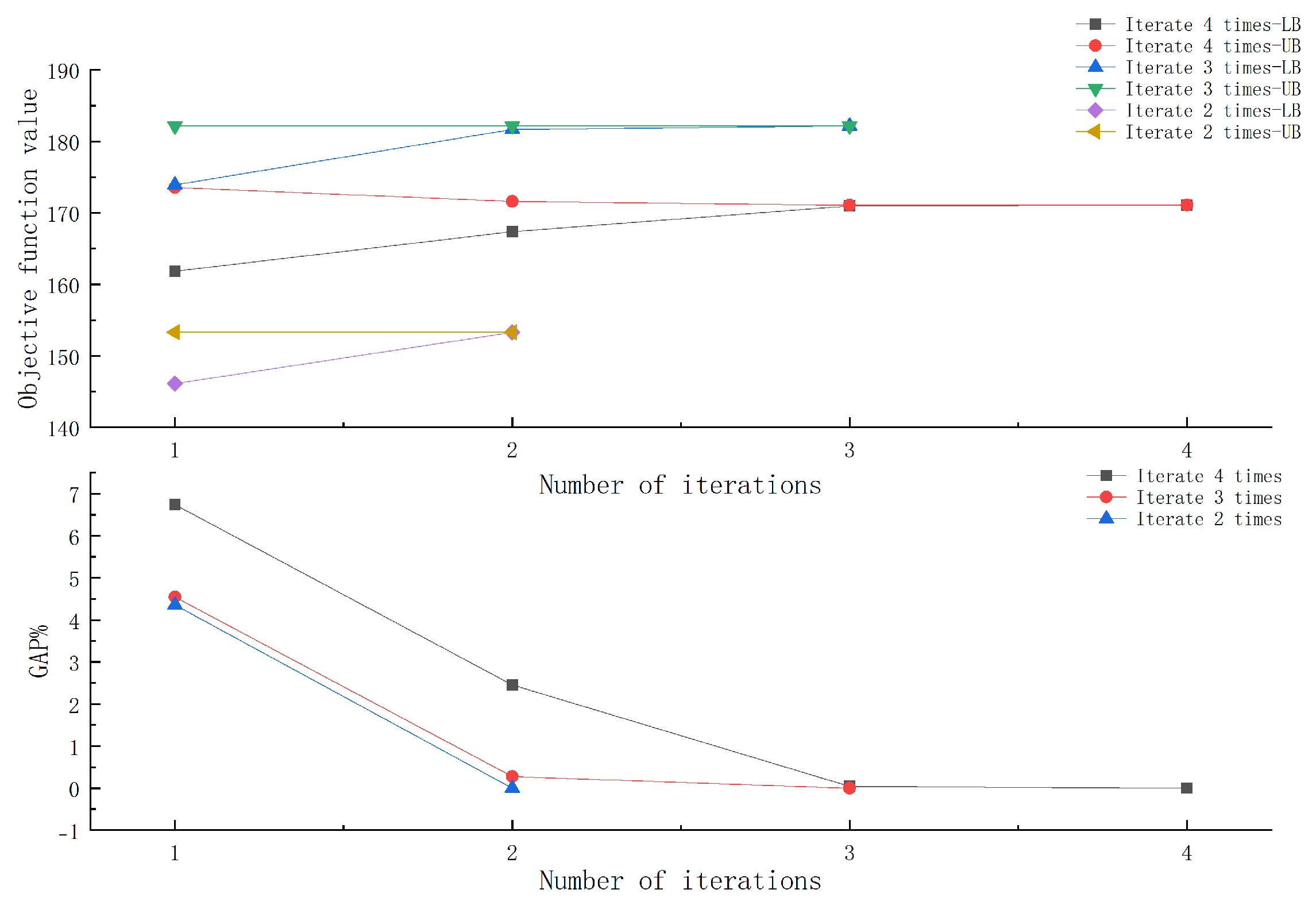
Figure 6 illustrates the changes in the objective function bounds and the Gap values with respect to the number of iterations under different task distribution scenarios. The upper panel shows the convergence process of the upper and lower bounds, while the lower panel presents the trend of the Gap values. The results indicate that, within a limited number of iterations, the upper and lower bounds gradually approach each other and eventually converge, and the Gap values continuously decrease toward zero. Three typical convergence cases are shown in the figure, corresponding to three independent scenarios in which the algorithm converges after 2, 3, and 4 iterations, respectively.

Figure 6. Iterative convergence process.

For scenarios converging after 2 iterations, the upper bound remains stable, while the lower bound rapidly rises and coincides with the upper bound at the end of the iteration. This occurs because the initial UAV-BS deployment scheme is already optimal and requires no further adjustment. Specifically, the lower bound is determined by the master problem based on the initial probability distribution, whereas the upper bound from the subproblem accounts for the worst-case probability distribution corresponding to the given deployment, and is therefore typically higher than the master problem’s lower bound. In the subsequent iteration, the worst-case distribution identified by the subproblem is added as a constraint to the master problem, which leads to the convergence of the bounds, confirming that the deployment is optimal. For scenarios converging after 3 or 4 iterations, the bounds do not converge in the early iterations, indicating that better deployment solutions may exist, allowing the upper bound to be further reduced until convergence is achieved. As more worst-case probability distribution scenarios are gradually incorporated into the master problem constraints, the model continuously optimizes the UAV-BS deployment, ultimately obtaining a more robust deployment strategy and ensuring convergence of the bounds, resulting in the optimal deployment solution. These results demonstrate that the proposed method can achieve stable convergence under different distributional perturbations while maintaining good computational efficiency and robustness.

5.2. Comparative Experiments

This subsection designs two sets of comparative experiments, all based on the publicly available inspection dataset from reference [16]. Given that the proposed TDRO method fundamentally differs from conventional optimization models assuming fixed inspection frequencies in terms of problem assumptions and modeling foundations, the experiments are conducted to systematically evaluate its performance from two perspectives: the effectiveness in modeling inspection frequency uncertainty and the capability to resist distributional perturbations. The first set of experiments aims to verify the method’s adaptability in multi-scenario dynamic inspection environments. By comparing a scheme that accounts for multi-scenario inspection frequency uncertainty with a scheme assuming constant inspection frequencies, the scheduling performance of the TDRO method under different inspection demand scenarios is evaluated. The second set of experiments further assesses the method’s effectiveness in enhancing robustness against disturbances. By comparing the decision performance of the TDRO method with that of the SO method under worst-case probability distribution scenarios, the experiments validate the TDRO method’s robustness in the presence of distributional perturbations.

Table 3 compares the experimental results under three scenarios of different scales. The results indicate that, in the presence of distributional perturbations, the proposed TDRO method significantly outperforms the traditional SO method under worst-case probability distribution scenarios, achieving an average reduction of 2.16% in the objective function. This advantage arises from the fact that TDRO takes worst-case probability distribution scenarios into account at the modeling stage, enabling a foresight-based UAV-BS deployment scheme that maintains high system performance when distributional perturbations occur. Moreover, when only inspection frequency uncertainty is considered, the TDRO method also outperforms deployment schemes assuming constant inspection frequencies, achieving an average reduction of 5.50% in the objective function.

Table 3. Comparative Experimental Results.

D	C	SO	DRO	Gap	Fixed Frequency	Frequency Uncertain	Gap
3	20	173.31	171.83	0.9%	174.17	166.44	4.5%
3	20	163.93	161.70	1.3%	165.00	157.17	4.7%
3	20	173.15	169.66	2.0%	178.07	168.37	5.4%
3	20	182.11	171.34	5.9%	184.40	177.01	4.0%
3	20	137.78	132.72	3.7%	151.90	136.40	1.0%
4	35	234.48	231.97	1.1%	249.43	243.99	2.2%
4	35	249.94	242.08	3.1%	251.18	251.18	-
4	35	242.17	234.29	3.2%	325.81	303.05	7.0%
4	35	259.62	254.89	1.8%	265.80	257.68	3.1%
4	35	281.30	276.63	1.7%	306.41	294.35	3.9%
5	55	334.39	328.09	1.9%	359.33	336.85	6.3%
5	55	365.57	362.85	0.7%	457.36	395.27	1.4%
5	55	330.42	325.06	1.6%	388.44	350.10	9.8%
5	55	337.35	337.35	-	446.68	367.92	17.6%
5	55	329.23	317.58	3.5%	406.43	359.09	11.6%

Specifically, in handling uncertainty across multiple inspection frequency scenarios, the model ensures high inspection efficiency for scenarios with higher probabilities and for tasks with higher inspection frequencies. By dynamically adjusting the deployment strategy, it reduces the expected inspection time across all scenarios in the objective function, thereby achieving efficient allocation of UAV resources. When the historical inspection data are relatively stable, TDRO and the SO method may yield identical results, since the existing deployment schemes in these cases are already sufficiently robust and require no further adjustment. However, the advantage of the TDRO model becomes more pronounced when distributional perturbations have a greater impact on the system. This is because the SO approach relies on a fixed historical probability distribution, which may deviate from actual inspection conditions. In contrast, the TDRO model explicitly incorporates worst-case distributional perturbations into the first-stage decision-making process, enabling a more foresighted deployment strategy. As a result, TDRO maintains better performance under distributional shifts and achieves improved robustness compared to the SO method. In summary, the TDRO model demonstrates strong effectiveness and adaptability under varying uncertainty conditions. By enhancing the robustness of the deployment scheme in response to both task uncertainty and distributional perturbations, it achieves a coordinated optimization of inspection efficiency and deployment cost within a unified optimization framework.

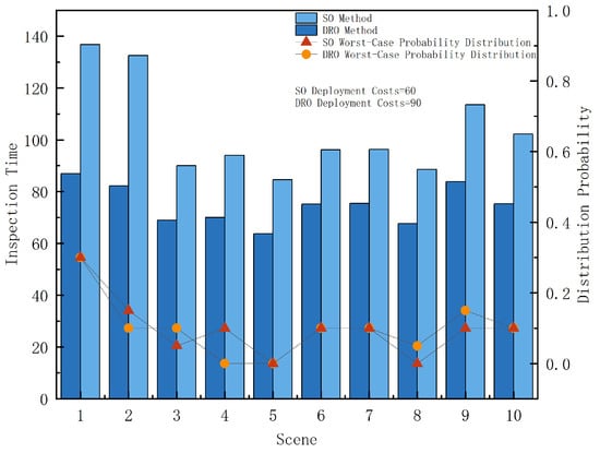
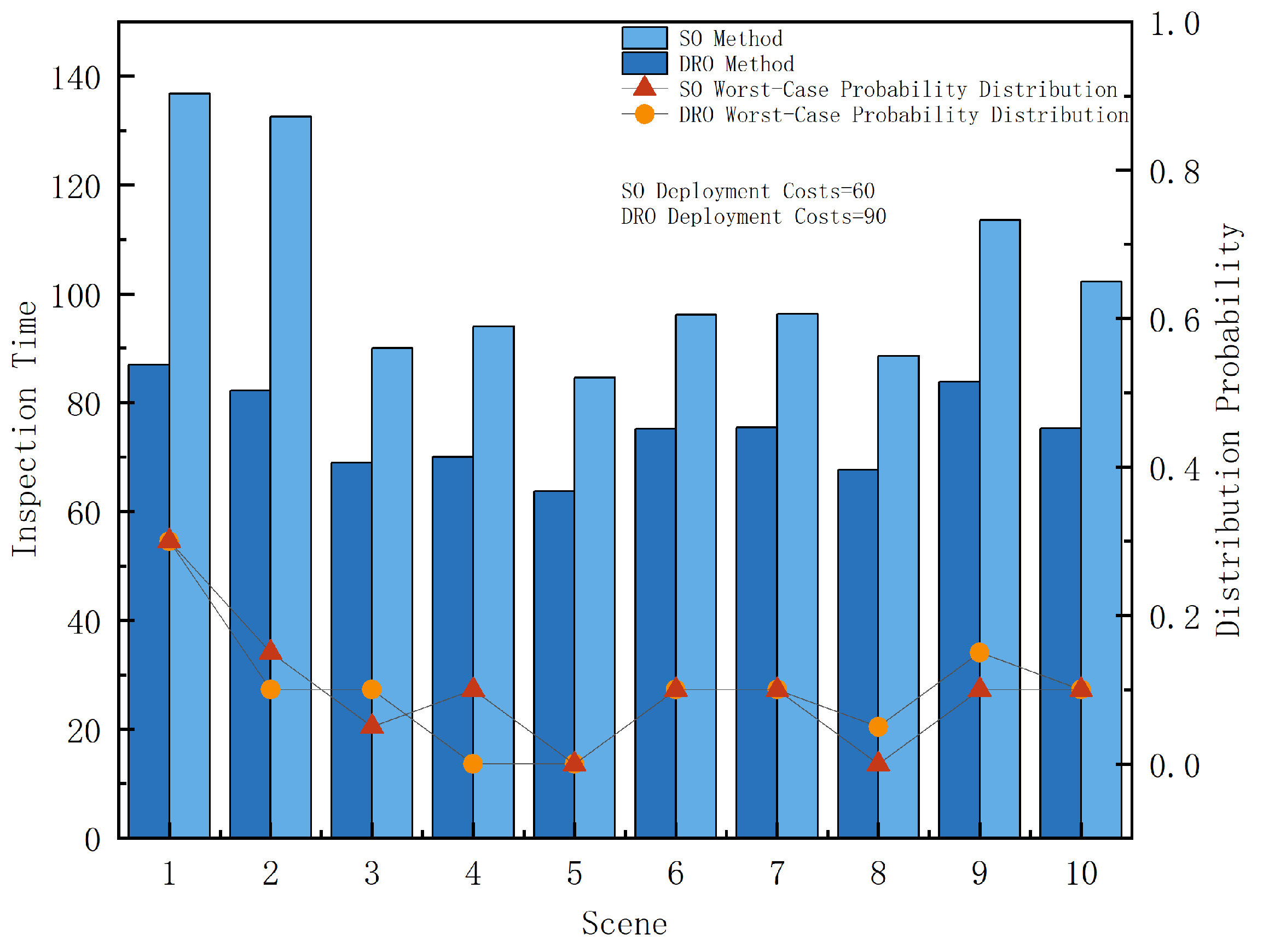
Figure 7 presents a comparison between the DRO method and the SO method for a set of instances in a scenario. The results indicate that by considering distributional perturbations, the DRO method is able to construct more robust UAV-BS deployment schemes. Although the deployment cost increases slightly in this scenario, the DRO method effectively shortens the inspection time of high-probability tasks by optimizing their execution paths, thereby reducing the overall inspection time and achieving a better overall objective value than the SO method. This is because the SO approach makes deployment decisions based on a fixed historical probability distribution. Once a distributional perturbation occurs, the probability of certain scenarios with long inspection times under the worst-case distribution may increase significantly, which can impact the overall system performance. In contrast, the DRO method proactively accounts for such potential distributional perturbations during the modeling stage, enabling a foresighted adjustment or reinforcement of the deployment scheme to ensure good expected performance of the overall objective function. Specifically, under the worst-case probability distribution scenarios, the DRO method readjusts the UAV-BS deployment scheme to effectively control the inspection time of key high-probability tasks that are most affected by distributional perturbations (such as Scenario 1 and Scenario 2), thereby improving the stability of the overall scheme and reducing the objective function value. These results demonstrate that the DRO method exhibits stronger adaptability in coping with uncertainty in probability distributions and can achieve superior overall performance at the global objective level.

Figure 7. Comparison of DRO and SO methods under a set of historical scenarios.

5.3. Experiments on Method Applicability

To validate the applicability of the proposed model and method across scenarios of different scales, we conduct computational experiments on a total of 30 scenarios, including small-, medium-, and large-scale cases, to analyze their performance under varying scales. In addition, further experiments are performed to investigate key parameters that may affect the computational efficiency of the model and method.

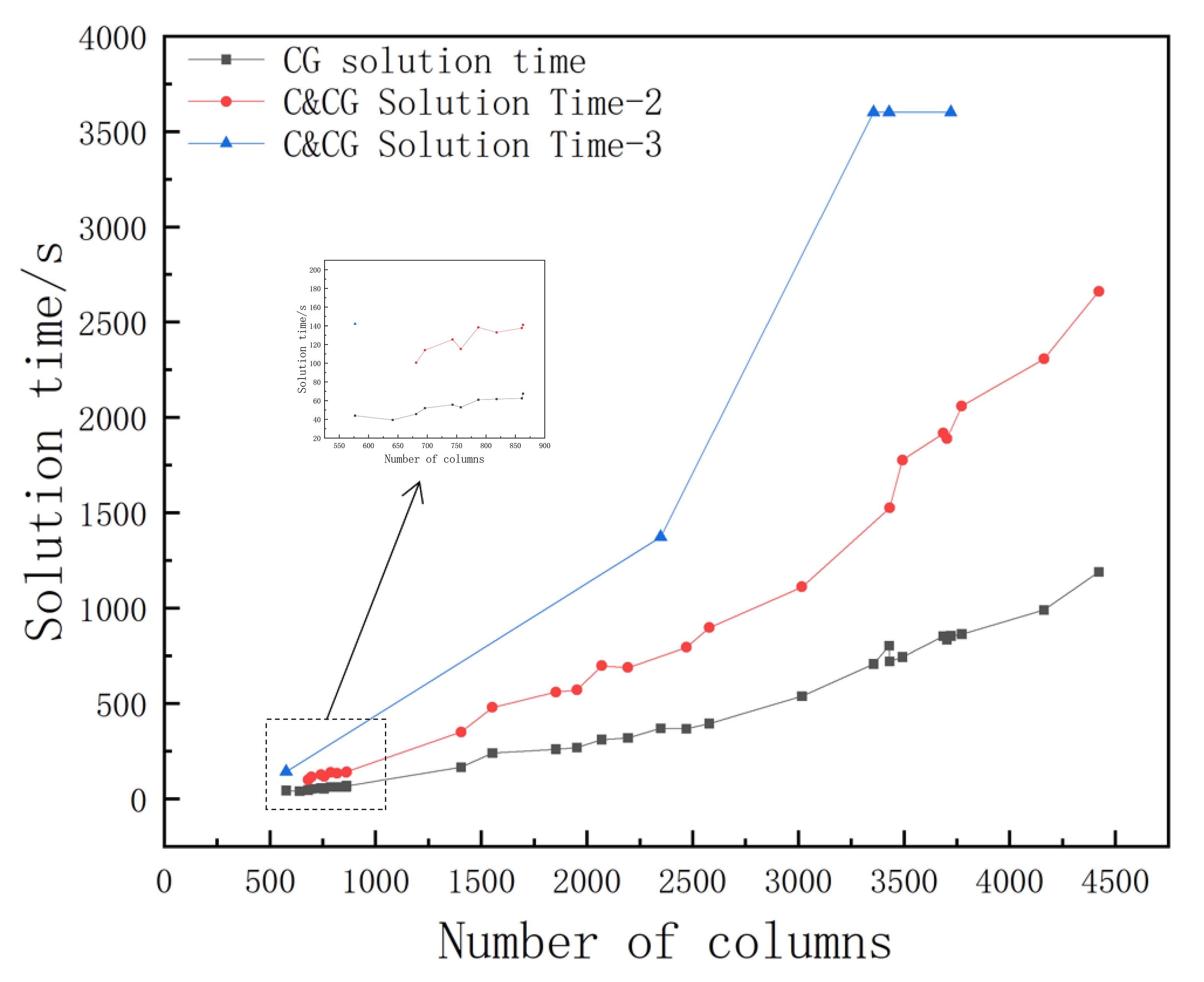
Table 4 presents the computational results for scenarios of different scales, including the number of columns generated, the CG algorithm solving time in the first iteration, the overall C&CG algorithm solving time, and the number of iterations (* indicates non-convergence within 3600 s). The results show that as the problem scale increases, the number of columns generated gradually rises, leading to a corresponding increase in the CG algorithm’s solving time. Similarly, the overall solving time of the C&CG algorithm also exhibits an increasing trend. Further analysis indicates that the overall solving time of the C&CG algorithm is significantly affected by the number of iterations. In terms of time composition, the main computational cost comes from solving the CG algorithm in each iteration, while the additional overhead introduced by the C&CG algorithm itself is relatively small. It is worth noting that although the CG solving time generally increases with the number of columns generated, monotonic growth is not observed in certain scenarios (e.g., Group 1 and Group 8). This is mainly because the CG algorithm’s path generation process is influenced by factors such as node spatial distribution and the number of inspection tasks, resulting in varying search difficulty across instances and, consequently, fluctuations in solving time.

Table 4. Computational instances under different scales.

D	C	Iterations	Number of Columns Generated	CG Solving Time/s	C&CG Solving Time/s	Converged
3	20	2	757	52.83	115.21	Yes
3	20	4	641	39.33	249.17	Yes
3	20	2	863	67.45	140.89	Yes
3	20	2	787	60.95	138.31	Yes
3	20	2	696	52.01	113.96	Yes
3	20	3	577	43.99	141.97	Yes
3	20	2	818	61.69	132.98	Yes
3	20	2	743	55.64	170.61	Yes
3	20	2	861	62.50	137.65	Yes
3	20	2	681	45.67	100.52	Yes
4	35	2	1853	260.46	559.03	Yes
4	35	2	2470	366.54	793.53	Yes
4	35	2	1953	268.9	569.94	Yes
4	35	2	2579	394.97	896.73	Yes
4	35	2	1553	239.56	478.64	Yes
4	35	2	2194	319.25	687.50	Yes
4	35	2	2070	310.05	698.01	Yes
4	35	3	2349	369.92	1372.43	Yes
4	35	2	3017	537.54	1110.76	Yes
4	35	2	1405	164.92	349.87	Yes
5	55	2	4422	1189.16	2661.97	Yes
5	55	2	4162	990.28	2307.17	Yes
5	55	2	3703	834.42	1888.39	Yes
5	55	3	3430	802.461	*	No
5	55	2	3493	742.86	1775.97	Yes
5	55	2	3432	720.82	1525.40	Yes
5	55	3	3356	706.76	*	No
5	55	2	3687	852.248	1917.03	Yes
5	55	3	3721	853.55	*	No
5	55	2	3773	864.14	2059.85	Yes

* indicates non-convergence within 3600 s.

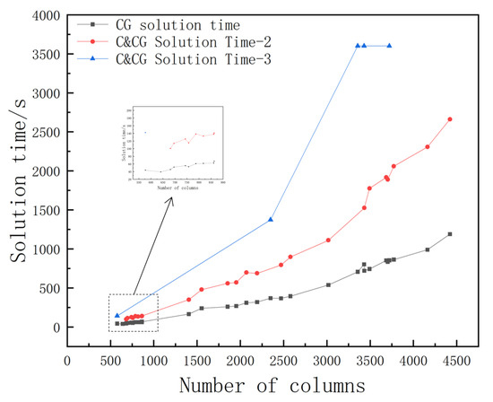
Figure 8 illustrates the impact of the number of columns generated on the CG algorithm’s solving time in the first iteration and on the overall C&CG algorithm’s solving time for iteration counts of 2 and 3. Overall, as the number of columns generated increases, the solving times of both algorithms show an upward trend. However, fluctuations in solving time are observed in some scenarios due to differences in the spatial distribution of inspection task points. When task points are more concentrated, the algorithm needs to handle more feasible paths during the search process, leading to increased computational time. In addition, as the number of iterations increases, the overall solving time of the C&CG algorithm also increases. This is mainly because the C&CG algorithm decomposes the original problem into master and subproblems to solve deterministic scenarios, thereby reducing overall complexity, while the additional computational overhead introduced by the algorithm itself remains insignificant.

Figure 8. Impact Please let us know if further adjustments are needed. of the number of columns on the algorithm solving time.

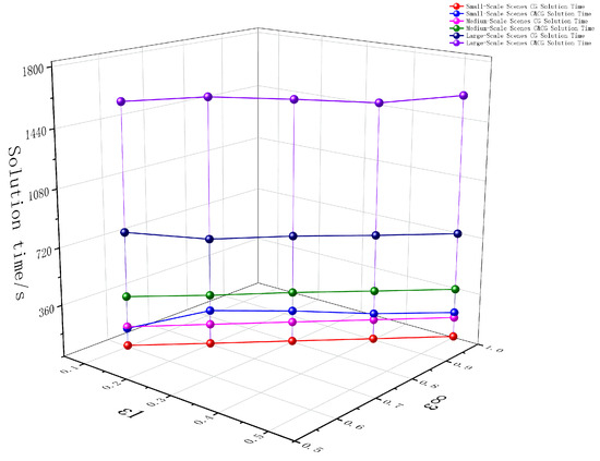
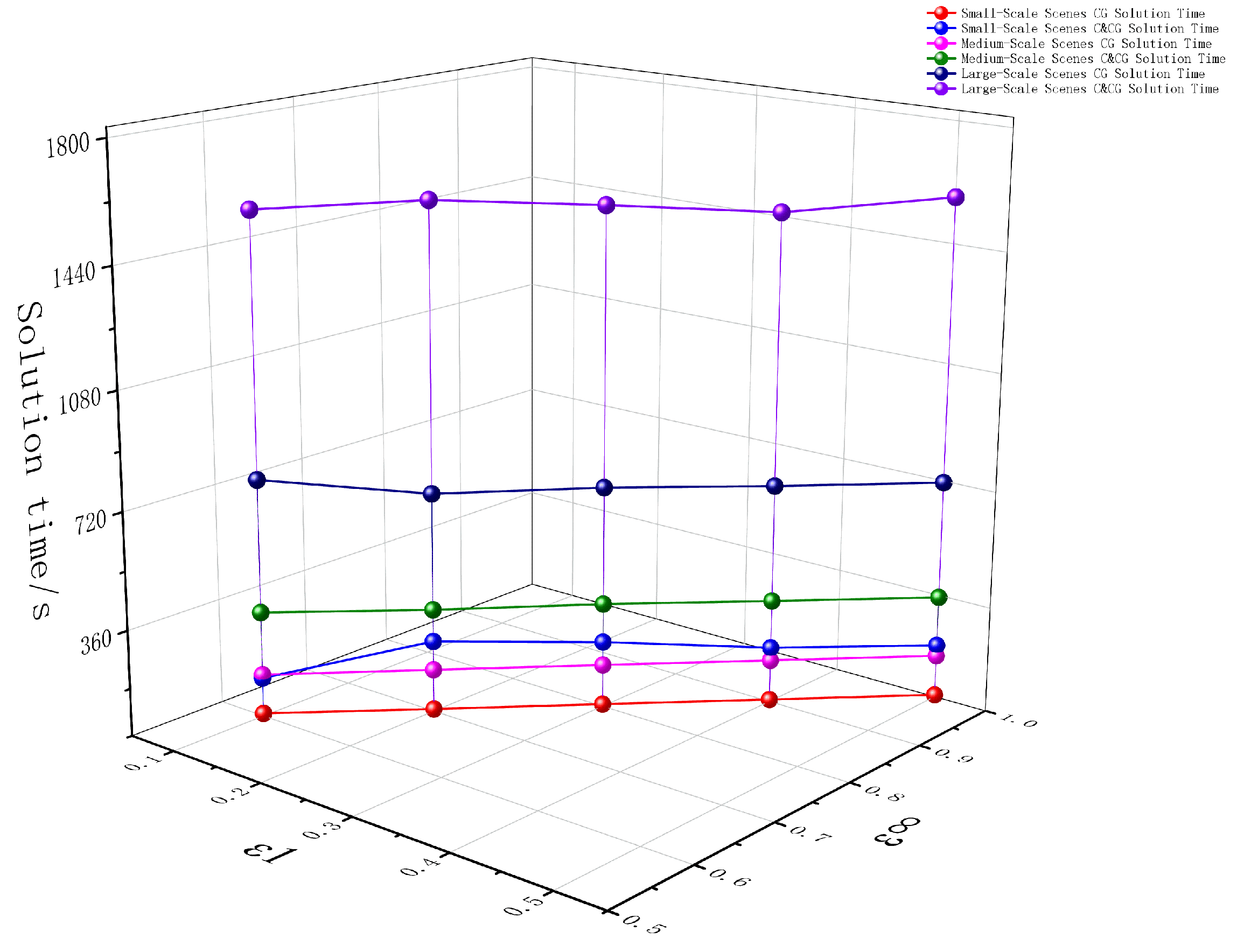
Figure 9 illustrates the impact of varying the $L_1$ norm and $L_{\infty }$ norm tolerance values on the solving time across three sets of experiments with different problem scales. The results show that the CG algorithm’s solving time remains relatively stable under different tolerance values, whereas the overall solving time of the C&CG algorithm fluctuates with changes in tolerance. Specifically, the CG algorithm’s solving time is largely unaffected because the tolerance constraints only restrict the range of probability distributions without altering the internal solving structure. In contrast, the C&CG algorithm reconsiders the worst-case probability distribution scenarios during each iteration based on the tolerance values, leading to variations in both the number of iterations and the solving time. From a decision-making perspective, the proposed model, by employing a hybrid-norm approach that jointly constrains the cumulative deviation ($L_1$) and extreme deviation ($L_{\infty }$) of the probability distributions, effectively reflects the system’s complex uncertainties while maintaining high computational efficiency, enabling precise management of distributional perturbations and efficient decision-making in complex inspection environments.

Figure 9. Impact of tolerance value on algorithm solving time.

5.4. Experiment on the Impact of Weight Levels

Table 5 presents the results of 15 experiments across three scenario scales and five different weight settings, aimed at analyzing the impact of weight on the performance of the deterministic model. The results indicate that as the weight increases, the overall deployment cost tends to rise. This is because a higher weight increases the proportion of the second-stage inspection time in the objective function, leading the model to allocate more resources to deployment to reduce overall inspection time. Specifically, the number of UAV-BSs increases with the weight, but additional UAV-BSs are only deployed if they can significantly improve overall system efficiency; when the efficiency gain is insufficient to offset the corresponding deployment cost, no additional UAV-BSs are selected.

Table 5. Deployment schemes and objective function values under different weight settings.

D	C	$\mathit{\rho }$	Deployment Selection	Deployment Cost	Objective Function Value
3	20	30	0	30	132.80
3	20	60	0	30	235.61
3	20	90	0, 1	60	323.80
3	20	120	0, 1	60	411.73
3	20	150	0, 1	60	499.66
4	35	30	0, 1	60	223.01
4	35	60	0, 1, 2	90	359.01
4	35	90	0, 1, 2, 3	120	488.8
4	35	120	0, 1, 2, 3	120	611.79
4	35	150	0, 1, 2, 3	120	734.73
5	50	30	0, 1, 2	90	299.80
5	50	60	0, 1, 2, 3	120	480.78
5	50	90	0, 1, 2, 3	120	661.17
5	50	120	0, 1, 2, 3	120	841.56
5	50	150	0, 1, 2, 3	120	1021.94

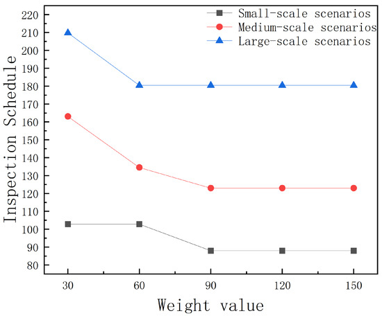
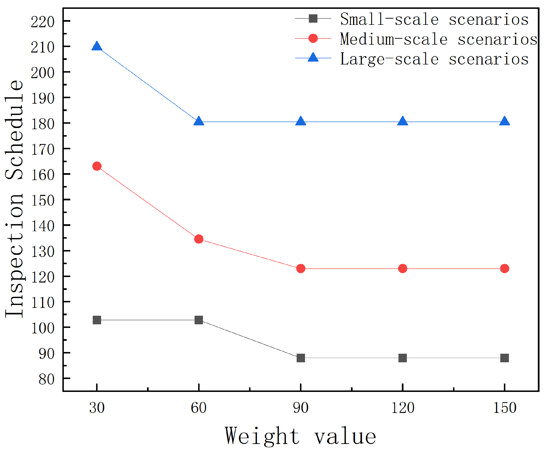
Figure 10 illustrates the impact of weight values on the expected second-stage inspection time. The results indicate that as the weight values increase, the model places greater emphasis on the second-stage inspection time, while the relative impact of deployment cost on the overall objective becomes less significant. As a result, the model tends to select deployment schemes that incur higher deployment costs in order to achieve lower inspection times. It is noteworthy that when the UAV-BS deployment scheme remains unchanged, variations in weight values do not affect the actual inspection time, as the weight values primarily influence decisions through deployment rather than directly altering task scheduling. This demonstrates that the proposed method is highly adaptable and can accommodate inspection requirements across different application scenarios. In practice, the weight values should be reasonably adjusted according to the scenario to achieve a proper trade-off between deployment cost and inspection time while avoiding unnecessary cost increases due to excessively high weight values.

Figure 10. Impact of weight values on inspection time.

6. Conclusions

This paper investigates the dynamic inspection problem of UAVs in large-scale infrastructure, with a focus on the coordinated optimization of UAV-BS deployment and inspection task scheduling. To address the dynamic variation in inspection task frequencies and the presence of distributional perturbations in historical data, a TDRO model is developed, and the C&CG algorithm is employed to solve the model’s uncertainty, while the CG algorithm is used to optimize inspection paths, achieving a coordinated optimization of deployment cost and inspection efficiency. The main conclusions are as follows:

(1) By considering the dynamic variation in inspection task frequencies and adaptively adjusting deployment schemes based on historical inspection data, high-probability tasks can be prioritized. Compared with deployment schemes assuming constant inspection frequencies, this strategy reduces the overall objective function by an average of 5.50%.

(2) The TDRO method effectively addresses perturbations in historical probability distributions. Through forward-looking adjustments to UAV-BS deployment, system performance remains stable even under distributional perturbations. Compared with the SO method based on empirical distributions, the overall objective is further reduced by an average of 2.16%.

(3) The TDRO method establishes a unified optimization framework that is applicable not only to fully deterministic inspection scenarios but also to environments with increasing uncertainty in inspection frequencies and distributional perturbations. The framework adaptively enhances the robustness of the deployment scheme, achieving a coordinated optimization of deployment efficiency and cost control in complex dynamic environments.

Future work may further incorporate additional real-world operational constraints, including UAV energy limitations (such as flight energy consumption, payload variations, and charging strategies), no-fly zone restrictions, weather conditions, and communication limitations. Considering these factors within a unified optimization framework would further enhance the realism, applicability, and decision-making feasibility of the proposed UAV inspection planning approach in practical engineering applications.

References

- Javid, Y. Efficient risk-based inspection framework: Balancing safety and budgetary constraints. Reliab. Eng. Syst. Saf. 2025, 253, 110519. [Google Scholar] [CrossRef] [Scilit]
- Nikolic, J.; Burri, M.; Rehder, J.; Leutenegger, S.; Huerzeler, C.; Siegwart, R. A UAV system for inspection of industrial facilities. In Proceedings of the IEEE Aerospace Conference, Big Sky, MT, USA, 2–9 March 2013; pp. 1–8. [Google Scholar] [CrossRef] [Scilit]
- Mohsan, S.A.H.; Othman, N.Q.H.; Li, Y.; Alsharif, M.H.; Khan, M.A. Unmanned aerial vehicles (UAVs): Practical aspects, applications, open challenges, security issues, and future trends. Intell. Serv. Robot. 2023, 16, 109–137. [Google Scholar] [CrossRef] [Scilit] [PubMed]
- Jacobsen, R.H.; Matlekovic, L.; Shi, L.; Malle, N.; Ayoub, N.; Hageman, K.; Hansen, S.; Nyboe, F.F.; Ebeid, E. Design of an Autonomous Cooperative Drone Swarm for Inspections of Safety Critical Infrastructure. Appl. Sci. 2023, 13, 1256. [Google Scholar] [CrossRef] [Scilit]
- Zhen, L.; Yang, Z.; Laporte, G.; Wen, Y.; Fan, T. Unmanned Aerial Vehicle Inspection Routing and Scheduling for Engineering Management. Engineering 2024, 36, 223–239. [Google Scholar] [CrossRef] [Scilit]
- Nooralishahi, P.; Ibarra-Castanedo, C.; Deane, S.; López, F.; Pant, S.; Genest, M.; Avdelidis, N.P.; Maldague, X.P.V. Drone-Based Non-Destructive Inspection of Industrial Sites: A Review and Case Studies. Drones 2021, 5, 106. [Google Scholar] [CrossRef] [Scilit]
- Liu, H.; Tsang, Y.P.; Lee, C.K.M.; Wu, C.H. UAV Trajectory Planning via Viewpoint Resampling for Autonomous Remote Inspection of Industrial Facilities. IEEE Trans. Ind. Inform. 2024, 20, 7492–7501. [Google Scholar] [CrossRef] [Scilit]
- Zhu, T.; Boyles, S.D.; Unnikrishnan, A. Two-stage robust facility location problem with drones. Transp. Res. Part C Emerg. Technol. 2022, 137, 103563. [Google Scholar] [CrossRef] [Scilit]
- Huang, S.; Liu, K.; Zhang, Z.-H. Column-and-constraint-generation-based approach to a robust reverse logistic network design for bike sharing. Transp. Res. Part B 2023, 173, 90–118. [Google Scholar] [CrossRef] [Scilit]
- Abbasi, S.; Moosivand, M.; Vlachos, I.; Talooni, M. Designing the Location–Routing Problem for a Cold Supply Chain Considering the COVID-19 Disaster. Sustainability 2023, 15, 15490. [Google Scholar] [CrossRef] [Scilit]
- Hassanpour, S.T.; Ke, G.Y.; Zhao, J.; Tulett, D.M. Infectious waste management during a pandemic: A stochastic location-routing problem with chance-constrained time windows. Comput. Ind. Eng. 2023, 177, 109066. [Google Scholar] [CrossRef] [Scilit]
- He, Y.; Liu, Z.; Guo, Y.; Zhu, Q.; Fang, Y.; Yin, Y.; Wang, Y.; Zhang, B.; Liu, Z. UAV based sensing and imaging technologies for power system detection, monitoring and inspection: A review. Nondestr. Test. Eval. 2025, 40, 5681–5748. [Google Scholar] [CrossRef] [Scilit]
- Luo, Y.; Yu, X.; Yang, D.; Zhou, B. A survey of intelligent transmission line inspection based on unmanned aerial vehicle. Artif. Intell. Rev. 2023, 56, 173–201. [Google Scholar] [CrossRef] [Scilit]
- Kon, T.E. The Importance of the Use of Unmanned Aerial Vehicles (UAVs) in the Oil and Gas Industry. Pet. Sci. Eng. 2024, 8, 63–69. [Google Scholar] [CrossRef] [Scilit]
- Chung, H.M.; Maharjan, S.; Zhang, Y.; Eliassen, F.; Strunz, K. Placement and Routing Optimization for Automated Inspection with Unmanned Aerial Vehicles: A Study in Offshore Wind Farm. IEEE Trans. Ind. Inform. 2021, 17, 3032–3043. [Google Scholar] [CrossRef] [Scilit]
- Cai, L.; Li, J.; Wang, K.; Luo, Z.; Qin, H. Optimal allocation and route design for station-based drone inspection of large-scale facilities. Omega 2025, 130, 103172. [Google Scholar] [CrossRef] [Scilit]
- Yan, Y.; Liang, Y.; Zhang, H.; Zhang, W.; Feng, H.; Wang, B.; Liao, Q. A two-stage optimization method for unmanned aerial vehicle inspection of an oil and gas pipeline network. Pet. Sci. 2019, 16, 458–468. [Google Scholar] [CrossRef] [Scilit]
- Zhang, H. Offshore Oilfield Inspection Planning with Drone Routing Optimization. IEEE Access 2024, 12, 20885–20893. [Google Scholar] [CrossRef] [Scilit]
- Xue, G.; Li, Y.; Wang, Z. Vessel-UAV Collaborative Optimization for the Offshore Oil and Gas Pipelines Inspection. Int. J. Fuzzy Syst. 2023, 25, 382–394. [Google Scholar] [CrossRef] [Scilit]
- He, X.; Zhong, Y.; Li, H. Distributed Robust Routing Optimization for Laser-Powered UAV Cluster with Temporary Parking Charging. Appl. Sci. 2025, 15, 9676. [Google Scholar] [CrossRef] [Scilit]
- Fang, Z.; Savkin, A.V. Strategies for Optimized UAV Surveillance in Various Tasks and Scenarios: A Review. Drones 2024, 8, 193. [Google Scholar] [CrossRef] [Scilit]
- Yang, Y.; Wu, W. A Distributionally Robust Optimization Model for Real-Time Power Dispatch in Distribution Networks. IEEE Trans. Smart Grid 2019, 10, 3743–3752. [Google Scholar] [CrossRef] [Scilit]
- Shui, Y.; Gao, H.; Wang, L.; Wei, Z.; Liu, J. A data-driven distributionally robust coordinated dispatch model for integrated power and heating systems considering wind power uncertainties. Int. J. Electr. Power Energy Syst. 2019, 104, 255–258. [Google Scholar] [CrossRef] [Scilit]
- Zeng, B.; Zhao, L. Solving two-stage robust optimization problems using a column-and-constraint generation method. Oper. Res. Lett. 2013, 41, 457–461. [Google Scholar] [CrossRef] [Scilit]
- Akca, Z.; Berger, R.T.; Ralphs, T.K. A Branch-and-Price Algorithm for Combined Location and Routing Problems Under Capacity Restrictions. In Operations Research and Cyber-Infrastructure; Chinneck, J.W., Kristjansson, B., Saltzman, M.J., Eds.; Springer: Boston, MA, USA, 2009; pp. 163–181. [Google Scholar] [CrossRef] [Scilit]
- Barreto, S.; Ferreira, C.; Paixão, J.; Santos, B.S. Using clustering analysis in a capacitated location-routing problem. Eur. J. Oper. Res. 2007, 179, 968–977. [Google Scholar] [CrossRef] [Scilit]
Disclaimer/Publisher’s Note: The statements, opinions and data contained in all publications are solely those of the individual author(s) and contributor(s) and not of MDPI and/or the editor(s). MDPI and/or the editor(s) disclaim responsibility for any injury to people or property resulting from any ideas, methods, instructions or products referred to in the content. |
© 2026 by the authors. Licensee MDPI, Basel, Switzerland. This article is an open access article distributed under the terms and conditions of the Creative Commons Attribution (CC BY) license.