


Featured Application
This study proposes an integrated framework for the prediction of embankment settlement and the prospective evaluation of its serviceability in permafrost regions, particularly under conditions of scarce monitoring data and dynamic, non-stationary settlement behavior. The developed SAA-GRU-LSTM hybrid model, combined with change-point detection, is designed to support infrastructure maintenance and risk management in cold regions engineering. It enables medium-term (e.g., 3–5 years) early-warning capability by utilizing only limited early-stage monitoring data to forecast settlement trends and assess compliance with safety standards. This approach is directly applicable to the health monitoring and decision-making for railway, highway, and other embankment structures built on degrading permafrost, helping to prioritize inspections, plan timely reinforcements, and evaluate the long-term effectiveness of cooling measures such as thermosyphons.
Abstract
Accurate prediction of embankment settlement and evaluation of its serviceability in permafrost regions are significantly challenged by scarce monitoring data and dynamic, non-stationary settlement processes. To address this, an integrated framework combining change-point detection with a novel dynamic prediction model is proposed. Analysis of long-term monitoring data from the Qinghai–Tibet Railway using the Pettitt test revealed a key change point around 2015, indicating a transition towards stabilization. Subsequently, an SAA-GRU-LSTM hybrid model, employing a dynamic compensation prediction strategy, was developed. The model successfully utilized only early-stage data to forecast future settlement trends, demonstrating robust performance in adapting to the identified abrupt change. Furthermore, by applying established engineering serviceability criteria to both historical and predicted data, the framework enables a dynamic and prospective serviceability assessment. This methodology provides a practical tool for the maintenance and risk management of infrastructure in permafrost environments under conditions of data scarcity and process uncertainty.
1. Introduction
Permafrost refers to soil or rock that remains at or below 0 °C for at least two consecutive years and contains ice [1]. It covers approximately 23% of the global land area and is primarily distributed in countries such as Russia, Canada, and China. Permafrost is highly sensitive to temperature disturbances, and under the influence of global climate warming, widespread and significant degradation of permafrost is occurring worldwide. Taking the Qinghai–Tibet Plateau (QTP) as an example, studies have shown that with an increase in mean annual air temperature of just 0.02 °C, the permafrost area on the plateau may decrease by 8.8% over the next 50 years. If the warming rate reaches 0.052 °C per year, the permafrost area is projected to shrink by 13.5% within the same period [2,3]. In addition to climate change, engineering activities can also lead to degradation of the underlying permafrost. As degradation progresses, the porosity and moisture content of the permafrost layer increase, resulting in soil consolidation and settlement under the self-weight of the overlying soil or surface loads [4].
The construction and maintenance of transportation infrastructure in permafrost regions face persistent challenges due to thaw-induced settlement, which directly threatens structural stability and operational safety [5]. Accurately predicting embankment settlement and evaluating its serviceability under such conditions is paramount for engineering design, risk management, and maintenance planning.
However, this task is significantly complicated by two inherent difficulties: the scarcity of physical information and the dynamic changes in the settlement process. Firstly, long-term, continuous geotechnical and thermal monitoring data in these remote and harsh environments are often limited, fragmented, or costly to obtain, resulting in “scarce physical information” for comprehensive model calibration and validation [6,7]. In this context, “scarce physical information” refers to the situation where only deformation monitoring has been carried out on the embankment, while no detailed monitoring or testing activities have been conducted for characteristics such as climate, ground temperature, hydrological conditions, and engineering geological conditions. Secondly, the settlement process is highly non-stationary [8]. It is influenced by the complex interplay of climate warming, the effectiveness of proactive cooling measures (e.g., thermosyphons, crushed-rock layers), and the inherent lag in the ground thermal response [9,10,11]. This leads to potential abrupt changes or trend shifts in settlement rates over time, which traditional prediction models, often assuming steady trends, fail to capture reliably [12].
Current research on permafrost embankment settlement has extensively focused on two aspects: the mechanisms of thaw-induced deformation and the cooling effectiveness of various engineering measures based on field monitoring or numerical simulation [13,14,15]. While these studies confirm the value of cooling measures, most prediction models are established under relatively ideal data conditions or for specific, stable phases. A critical gap remains in developing a robust prediction framework that can dynamically adapt to trend changes using only limited early-stage monitoring data (“scarce physical information”). Such a framework is essential not only for forecasting future settlement but also for the serviceability evaluation of embankments, as timely prediction of deformation trends is a direct indicator of whether the underlying permafrost and overlying structure are approaching a new equilibrium or a hazardous state.
To bridge this gap, this study proposes a novel dynamic prediction and evaluation approach. We utilize long-term settlement monitoring data from an embankment-bridge transition section along the Qinghai–Tibet Railway, reinforced with thermosyphons. First, the Pettitt test is employed to identify key change points in the settlement time series, explicitly addressing the “dynamic changes” in the process. Subsequently, we develop a hybrid time-series prediction model based on Gated Recurrent Unit (GRU) and Long Short-Term Memory (LSTM) networks, employing a dynamic compensation prediction strategy as its core framework. To enhance the model’s ability to search for the optimal solution in the complex parameter space, the Simulated Annealing Algorithm (SAA) is introduced to optimize the model’s hyperparameters. The SAA-GRU-LSTM model is designed to perform recursive, multi-step forecasting by iteratively incorporating its own predictions, thereby simulating and adapting to evolving trends even with limited initial data. The model’s outputs aim to achieve two interconnected goals: (1) accurate settlement prediction under conditions of data scarcity and process non-stationarity, and (2) a dynamic serviceability evaluation of the embankment by assessing whether predicted settlement trends comply with safety thresholds, thereby indirectly evaluating the long-term effectiveness of the cooling measures.
This study aims to provide a methodological framework that aligns directly with the challenges highlighted in the title—offering a practical solution for embankment settlement prediction and serviceability evaluation that consciously accounts for dynamic changes in the settlement process and operates effectively under constraints of scarce physical information.
2. Monitoring Site and Data Analysis
2.1. Monitoring Site Description
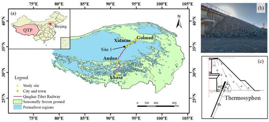
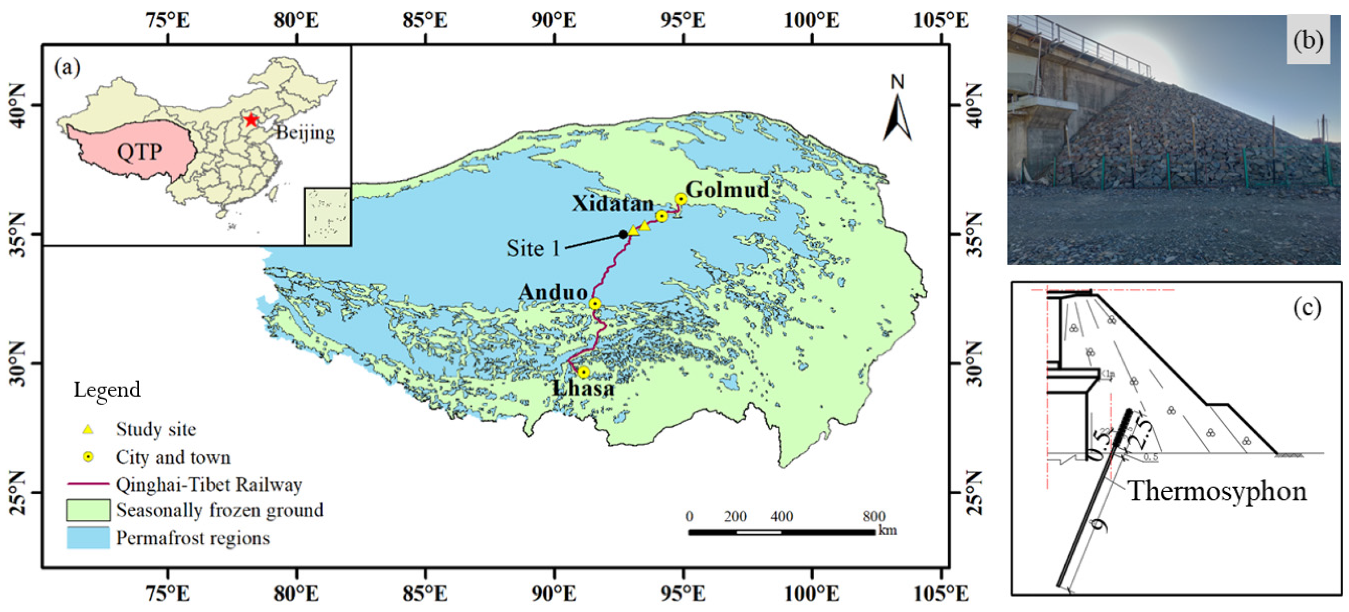
For this study, a monitoring site located at the embankment–bridge transition section (EBTS) on the Golmud side of one Bridge along the Qinghai–Tibet Railway (QTR) in the permafrost region was selected as the case study (location shown in Figure 1a). This monitoring site is situated at mileage DK1096+027, where the embankment height is approximately 10 m, the width is about 28 m, and the embankment orientation is 235° (with 0° indicating north), as shown in Figure 1b. This bridge was completed and opened to traffic in 2006. During construction, crushed-rock revetment was employed as a cooling measure for the embankment and abutment protection cone on the Golmud side EBTS. However, after four years of operation (around 2010), field investigations revealed significant settlement in the abutment and its protection cone, with settlement magnitudes clearly exceeding those observed in the adjacent embankment area. In response, thermosyphons were installed in 2010 in the significantly settling areas of the abutment and protection cone to suppress further deformation, while the embankment area retained the original crushed-rock revetment measure. Each thermosyphon is 9 m long and installed at a 22° angle to the ground at the edge of the abutment protection cone. Meanwhile, two settlement monitoring sections were established in both the embankment and abutment areas to continuously track deformation. Specifically, settlement monitoring points were set at the left and right shoulders of each monitoring section, along with a deeply embedded reference point at a depth of 20 m. The embankment settlement was determined by measuring the vertical displacement of monitoring points relative to this deep reference point. Elevation changes were measured manually using a leveling instrument, with a monitoring frequency of once per month. The dataset analyzed in this study consists of long-term settlement monitoring records covering the period from May 2010 to May 2020.
Figure 1.
(a) Location of monitoring site in the Qinghai–Tibet Plateau. The data in this map are from the Environmental and Ecological Science Data Center for West China; (b) photograph of the embankment–bridge transition section; (c) cross-section diagram of thermosyphon installation.
2.2. Settlement Characteristics and Dynamic Change Points
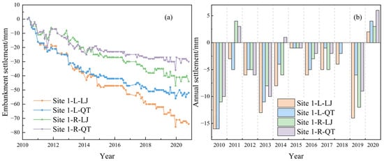
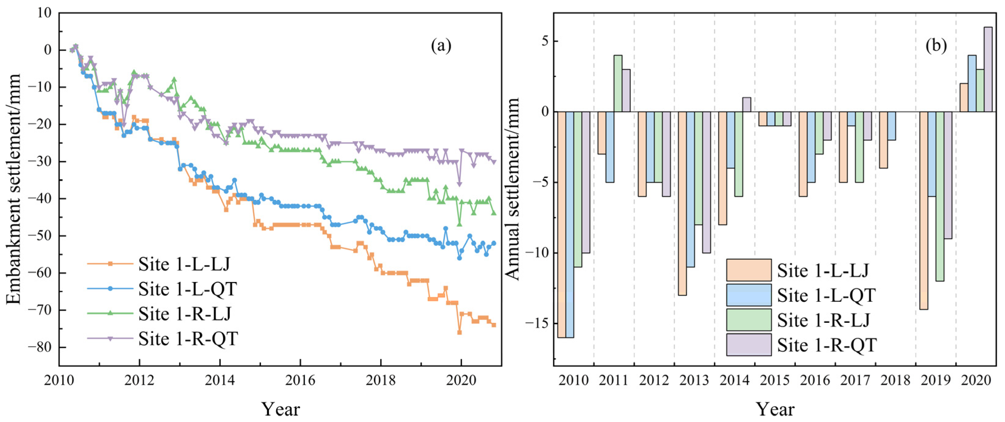
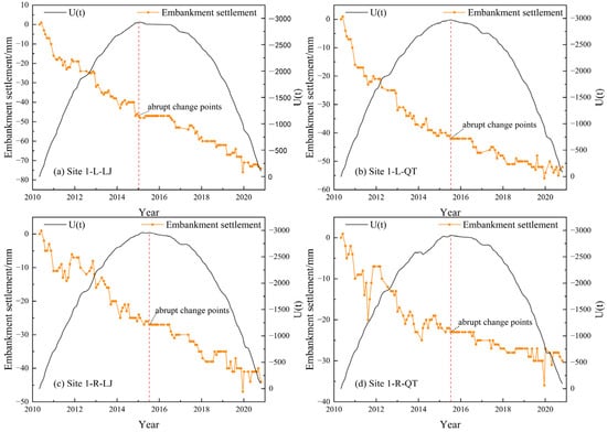
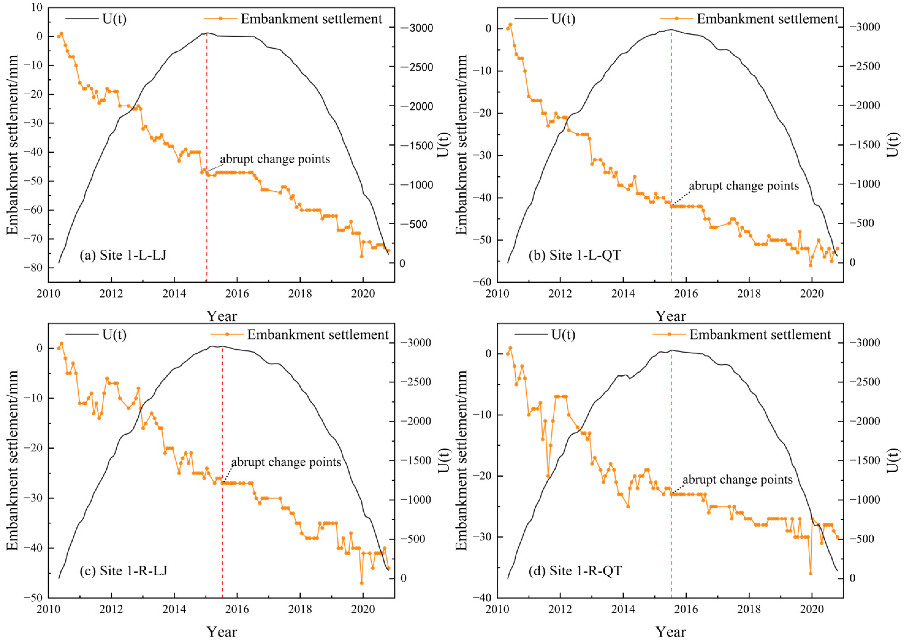
As shown in Figure 2a, all four monitoring points at Site 1 (Site 1-L-LJ, Site 1-L-QT, Site 1-R-LJ, and Site 1-R-QT; L: left; R: right; LJ: embankment; QT: abutment) experienced noticeable settlement starting from May 2010. The initial settlement rates were relatively high, which can be attributed to the thermal disturbance caused by the installation of thermosyphons at the abutment and protection cone during that year. Subsequently, the settlement trends gradually stabilized. Figure 2b presents the annual settlement at the four monitoring points after thermosyphon reinforcement. It can be observed that differences in settlement exist between the embankment and abutment as well as between the left and right sides, which is likely related to the north–south orientation of the embankment and the resulting shady–sunny slope effect. In general, the left side of the abutment tends to exhibit more pronounced settlement deformation than the right side; however, the differential settlement at the abutment is smaller than that at the embankment, as the thermosyphons were mainly installed around the abutment.
Figure 2.
(a) Cumulative settlement at each monitoring section; (b) annual settlement at each monitoring point. L: left; R: right; LJ: embankment; QT: abutment.
In the years immediately following reinforcement, the annual settlement of all four monitoring points at Site 1 shows a decreasing trend and reaches a minimum around 2015. Overall, during the period from 2010 to 2020, the annual settlement at both the embankment and abutment remained below 20 mm. This is because the monitoring sections are located in the transition zone between the abutment and the embankment, and the cooling effect of the thermosyphons extends into the embankment area, reducing the settlement trend of the underlying permafrost layer.
To investigate the key time point when the thermosyphons begin to exhibit a significant effect, the Pettitt test was applied to the settlement monitoring data to determine the change point in settlement rates. The Pettitt test is a non-parametric method used to detect abrupt changes in time series without prior knowledge of the change point, and to evaluate the statistical significance of the detected change. This method is advantageous due to its simplicity, robustness, and resistance to the influence of outliers. It is used here to determine how long after thermosyphon installation the reinforcing effect becomes statistically evident. The principle involves constructing a rank-based sequence for a time series X of n data points [16]:
In this method, the rank sequence Sk represents the cumulative number of instances where the value at time i is greater than or less than the value at time j. If the time point t0 satisfies the condition then t0 is identified as the abrupt change point in the time series.
Finally, the p-value is calculated as follows to evaluate the statistical significance of the result:
where a p-value p ≤ 0.05 indicates that the detected change point is statistically significant.
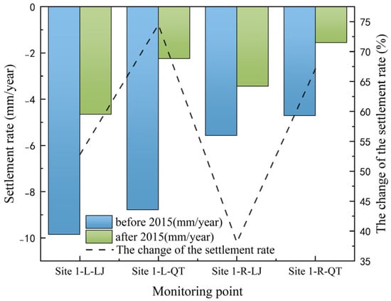
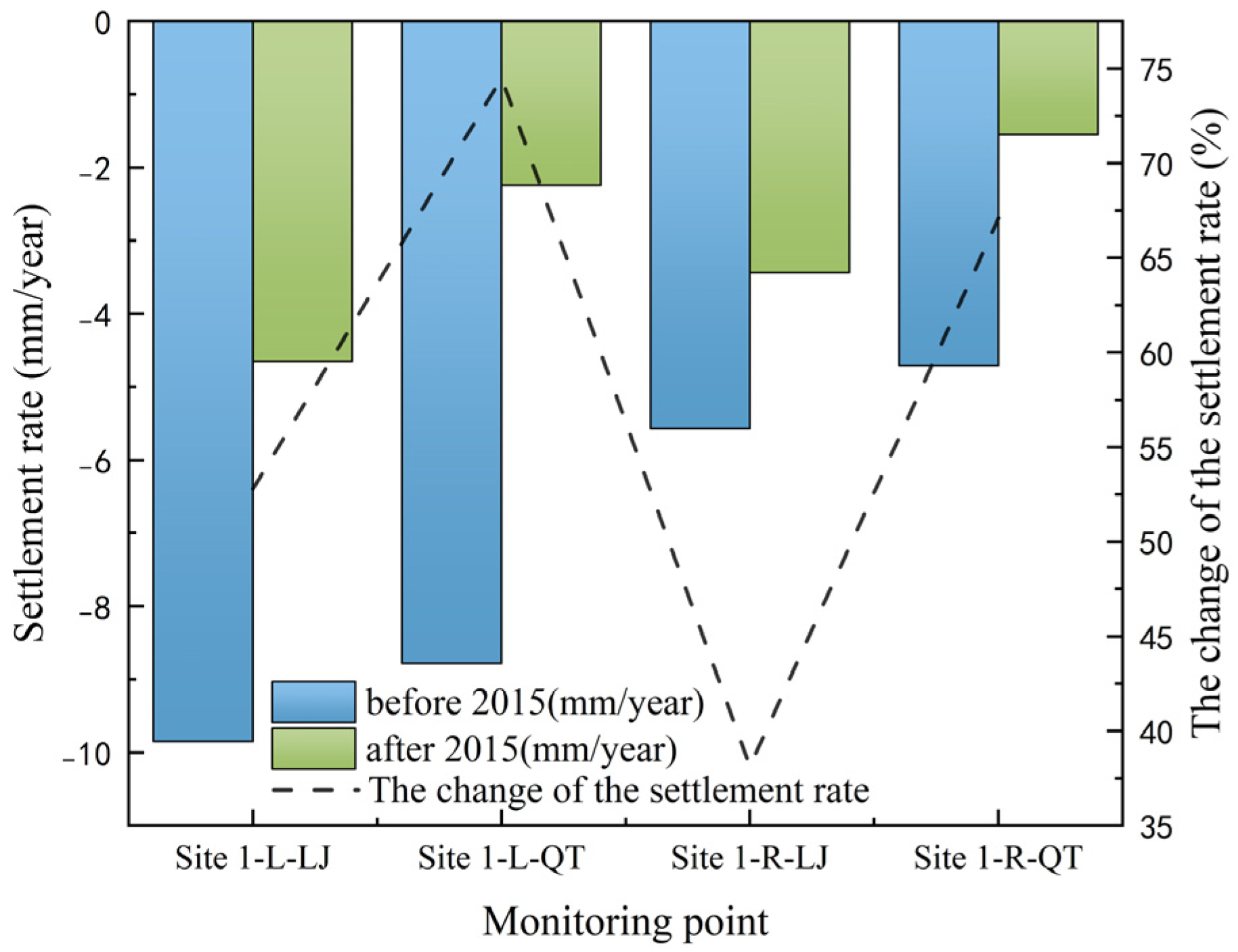
The results (Figure 3) reveal that statistically significant change points (p < 0.05) occurred around 2015 for all four monitoring points. This confirms the non-stationary nature of the settlement process, characterized by a significant shift in trend around this period. Comparative analysis of the interannual settlement rates before and after the 2015 change point (Figure 4) shows a marked reduction post-2015. For instance, at point Site 1-L-QT, the settlement rate decreased from 8.78 mm/year to 2.24 mm/year (a 74.5% reduction). The least pronounced change occurred at Site 1-R-LJ, where the rate still declined from 5.57 mm/year to 3.44 mm/year (a 38.1% reduction). This widespread deceleration in settlement after 2015 indicates a system-wide transition towards a more stable deformation regime.
Figure 3.
Results of the Pettitt change-point detection test.
Figure 4.
Changes in settlement rates before and after the detected change points.
Although the thermosyphons were installed in 2010, the significant reduction in settlement rates did not manifest until 2015, indicating a certain time lag in their cooling effect on the underlying soil. The concentration of change points around 2015 reflects the progressive alteration of the subsurface thermal regime as a result of sustained thermosyphon operation. The pronounced cooling observed after 2015 significantly mitigated the trend of permafrost degradation. This five-year lag in effectiveness release confirms that the cooling mechanism of thermosyphons relies on the gradual accumulation of cold energy. Through efficient heat exchange, the thermosyphons progressively restore the thermal balance of the permafrost, substantially reducing the settlement associated with permafrost thaw.
2.3. In-Period Serviceability Evaluation Based on Monitoring Data
According to the Code for Design of Railway Embankments in China, a stable embankment for a Class I railway must meet the following criteria after completion: the accumulated settlement should be less than 200 mm, or the settlement rate should be less than 50 mm/year [17]. In practical engineering scenarios, if the continuous annual settlement rate exceeds 20 mm/year, reinforcement of the EBTS is required to ensure the safety of train operations. Therefore, the deformation observed at this monitoring site complies with the requirements of the railway embankment design code in China. These findings indicate that thermosyphons, as a surface cooling measure, are effective in inhibiting the degradation of underlying permafrost and thereby reducing the settlement of overlying engineering structures.
Based on the settlement monitoring data from 2010 to 2020, an in-period serviceability evaluation of the embankment was conducted against the design code criteria. For the entire monitoring period, the embankment demonstrated compliance with both key serviceability indicators. The total measured cumulative settlement for all points remained well below the 200 mm limit (Figure 2a), satisfying the code’s deformation control criterion. Furthermore, the maximum observed annual settlement rate across all points was below 20 mm/year (Figure 2b), which is not only under the operational concern threshold but also significantly lower than the 50 mm/year code limit, thereby meeting the rate-based requirement.
The identification of a statistically significant change point around 2015 necessitates a phase-based evaluation that acknowledges the dynamic nature of the settlement process. Prior to 2015, the embankment, while stable, exhibited higher settlement rates, indicating a period of more active but still controlled deformation. Following the 2015 transition, a marked reduction in settlement rates was observed across all monitoring points. This shift signifies that the embankment entered a state of enhanced serviceability, with deformation trends visibly converging toward a new equilibrium.
In conclusion, throughout the decade-long monitoring period from 2010 to 2020, the embankment at the studied site maintained overall serviceability as all measured performance indices complied with the stipulated design standards. The key dynamic characteristic captured was a transition around 2015 from a state of active settlement to one of significantly attenuated deformation. This evolution likely reflects the delayed, yet positive, influence of the thermosyphon reinforcement installed in 2010, which ultimately contributed to an improved serviceability condition in the latter half of the observed timeframe.
3. Settlement Prediction and Serviceability Evaluation
3.1. Method
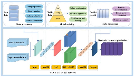
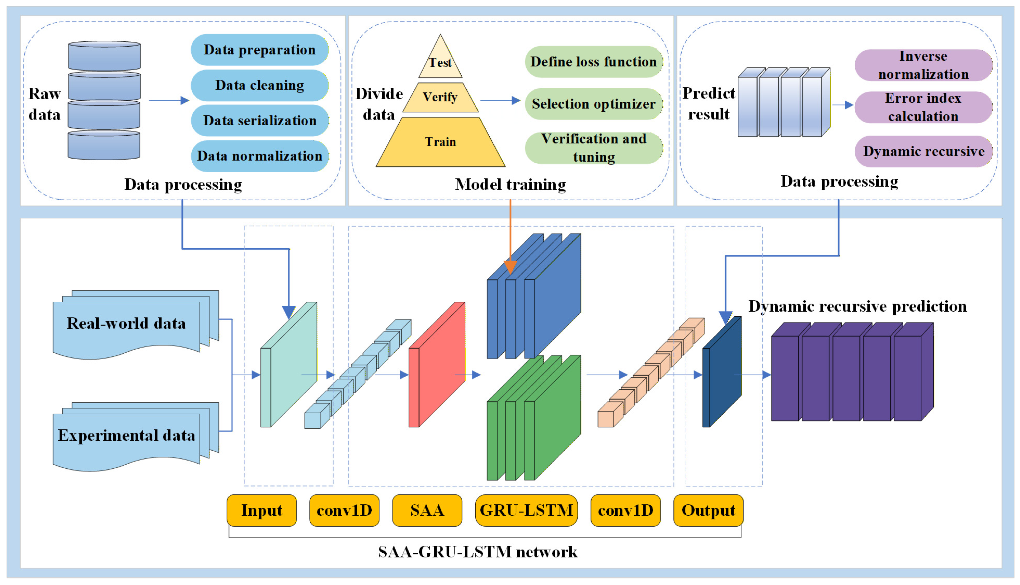
In permafrost regions, embankment settlement is influenced by various factors, including climatic conditions, engineering geological settings, and structural design types. These factors lead to significant uncertainty in the settlement process and often result in abrupt changes in settlement trends [18]. Such non-stationary variations pose a challenge for conventional machine learning prediction models, which typically assume stable trends [19]. Traditional models tend to capture the dominant pre-change patterns during training, and as a result, even when post-change data is included, their predictions often continue to reflect pre-change trends [20]. This leads to systematic bias and significantly increased error in predictions made after abrupt changes. To address this limitation, the SAA-GRU-LSTM hybrid time-series dynamic compensation prediction model proposed in this study is designed to accommodate the characteristics of settlement trend changes. It adopts a stepwise, phase-based recursive modeling strategy to gradually correct the prediction path and achieve smooth trend transition. This approach reduces reliance on the original full-length dataset, thereby improving the model’s generalizability and fitting capability [21]. The hybrid model is constructed based on the TensorFlow and Keras frameworks and is specifically designed to handle nonlinear, long-term dependent settlement sequences [22]. The model architecture integrates both GRU and LSTM recurrent neural network units, each with three hidden layers to enhance its ability to learn complex data patterns. The overall model architecture is illustrated in Figure 5, and key hyperparameter configurations are listed in Table 1.
Figure 5.
SAA-GRU-LSTM hybrid model architecture.
Table 1.
Hyperparameter Configuration of LSTM and GRU Components.
To enhance the model’s ability to search for the optimal solution in a complex solution space, the SAA was introduced. SAA is a stochastic optimization method based on Monte Carlo iteration, with its core concept derived from the thermodynamic principles of the metal annealing process in solid physics [23]. By setting a high initial temperature and gradually cooling down, SAA accepts worse solutions with a relatively high probability during the early search phase, enabling it to escape local optima; as the temperature decreases, the search gradually converges, ultimately achieving a global optimum [24]. The Metropolis criterion is used to control the acceptance probability of new solutions, thus ensuring the global optimization capability of the algorithm [25]. The calculation of the “certain probability” here references the annealing process in metal smelting. We treat the temperature T as a control parameter and the objective function as the internal energy E, while a state of the solid at a given temperature corresponds to a solution (Xi). The algorithm then attempts to lower the control parameter Tso that the objective function F (i.e., internal energy E) gradually decreases, eventually converging to the global minimum, akin to the lowest energy state achieved during the low-temperature phase of metal annealing. The specific mechanism for updating solutions is as follows: if a new solution is superior to the current one, it is accepted; otherwise, acceptance is determined based on the Metropolis (Monte Carlo) criterion. The probability of accepting a solution during each update is given by the following formula [26]:
In this way, the algorithm can explore a larger search space in the early stages and focus more on finding the optimal solution in the later stages, making it particularly well-suited for solving complex problems with multiple local optima.
In this hybrid architecture, the core sequence modeling components consist of LSTM and GRU. The LSTM network includes three types of gates: the forget gate (Ft), input gate (It), and output gate (Ot), each governed by the following equations [27]:
The forget gate determines how much information from the previous state should be discarded at the current time step to prevent interference from long-term irrelevant information:
The input gate controls the influence of the current input on the state update, deciding which parts of the current input need to be written into the memory cell:
The output gate decides how much memory information from the current hidden state is outputted to be passed on to the next time step or the final output:
The nonlinear output is then calculated based on the above output and input:
Finally, the new cell state can be represented as:
where Wxi, Wxf, Wxo, Wxc and Whi, Whf, Who, Whc are weight parameters, bi, bf, bo, bc is a bias parameter, Xt is the input at time step t, σ and tanh are activation function, Ht−1 represents the output at time step t − 1, and × denotes element-wise multiplication.
The GRU introduces a reset gate and an update gate to control the flow of information, effectively alleviating the vanishing gradient problem commonly encountered by traditional Recurrent Neural Networks (RNNs) when processing long sequences. This enhances the model’s ability to capture long-term dependencies. The state update mechanism of GRU is defined as follows [28]:
where Wz, Wr is a weight parameter and bz, br is a bias parameter, Ht−1 represents the output at time step t − 1, and × denotes element-wise multiplication.
LSTM and GRU each have their own advantages in terms of modeling capacity and computational efficiency: LSTM excels at capturing long-term dependencies, whereas GRU offers faster training speed and lower memory consumption. Therefore, this study proposes a hybrid neural network that integrates both LSTM and GRU structures to simultaneously leverage their strengths in sequence modeling. This fused architecture not only enables the learning of richer temporal features but also improves model accuracy and computational efficiency by reducing the number of parameters, thus exhibiting superior predictive performance and broader applicability. To enhance the model’s ability to search for the optimal solution in a complex solution space, the SAA is introduced. SAA is a stochastic optimization technique based on Monte Carlo iteration, and its core concept is derived from the thermodynamic principles of the metal annealing process in solid-state physics. By setting a high initial temperature and gradually cooling down, SAA accepts inferior solutions with relatively high probability in the early search phase, thereby allowing the algorithm to escape from local optima. As the temperature decreases, the search becomes more refined, ultimately converging to the global optimum. The Metropolis criterion is employed to control the acceptance probability of new solutions, thereby ensuring the global optimization capability of the algorithm.
The ultimate objective of the SAA-GRU-LSTM dynamic prediction model developed in this study is to serve the serviceability evaluation of the embankment. The evaluation will be conducted in accordance with the dual-control criteria for the serviceability of Class I railway embankments, as stipulated in the Chinese Code for Design of Railway Embankments, and in conjunction with practical engineering management practices. Therefore, the model’s output—future settlement predictions (including both accumulated settlement and annual settlement rates)—will be directly compared against these thresholds. By assessing whether the predicted settlement trends comply with the code requirements, a dynamic and prospective serviceability evaluation of the embankment structure can be achieved. This, in turn, provides a quantitative basis for assessing the long-term effectiveness of the cooling measures.
3.2. Model Evaluation Metrics
Considering the influence of dimensionality on the use of mean squared error (MSE), employing the RMSE is more meaningful. This study adopts common machine learning evaluation metrics: the RMSE and MAPE [29]. The specific formulas are derived as follows:
The RMSE, as defined by the equation below, calculates the difference between predicted and actual values. A smaller RMSE value indicates a better fit of the predictive model and higher accuracy, commonly used in regression model evaluation.
The MAPE, defined by the equation below, measures the average percentage error between predicted and actual values, providing a realistic reflection of prediction accuracy. A smaller MAPE indicates better predictive performance of the model.
where n denotes the number of samples, yi represents the true values, and stands for the predicted values.
3.3. Data Description and Preprocessing
Monitoring was conducted from May 2010 to May 2020, totaling 109 months, to assess settlement deformations at EBTS. Due to missing data in certain months during monitoring, cubic spline interpolation was employed to obtain complete monthly datasets for the entire monitoring period. This method not only better depicts underlying data patterns but also mitigates the impact of noise or outliers in the raw data on the model, enabling improved capture of inherent data characteristics and enhancing model performance. Ultimately, data spanning May 2010 to May 2020, totaling 120 months with 4 sets of settlement monitoring data, each comprising 3653 samples, was obtained.
According to research recommendations [29], each dataset was partitioned such that the training data comprised 70–80% of the total dataset. In this study, each model training iteration divided the dataset into 80% for training, 10% for validation, and 10% for testing. To enhance the learning and convergence speed of the LSTM model and prevent overfitting, the monitored settlement deformation sequences (x1, x2, x3 ⋯ xt) were normalized to [0, 1], Subsequently, the entire dataset was predicted, and the output results were inverse-normalized. When dealing with time series characterized by non-stationarity and abrupt changes, traditional single models often struggle to maintain high prediction accuracy across the entire sequence. To address this issue, this study introduces a dynamic compensation prediction method. The core idea is to divide the entire sequence into multiple adjacent or overlapping time segments and perform phase-wise modeling and prediction using a sliding window approach. At each stage, the latest prediction results are incorporated into the input of the subsequent stage, forming a recursive and updating temporal structure. This method not only enables rapid adaptation to changes in data distribution but also reduces the reliance on global stationarity, thereby significantly improving the continuity and robustness of prediction results before and after mutation points. Ultimately, through the established SAA-GRU-LSTM hybrid time-series prediction model, continuous dynamic predictions of future embankment settlement were made. The specific research findings are presented below.
3.4. Determining the Size of the Dynamic Recursive Prediction Window
The presence of mutation points directly affects the rationality of dataset partitioning and the generalization capability of predictive models. In conventional modeling approaches, the training and testing sets are typically divided based on a fixed time ratio across the entire sequence. However, when a mutation point spans both the training and testing sets, or occurs entirely after the training set, the model fails to learn the mutation behavior during training, which severely weakens its ability to accurately predict future trends in the testing phase. This problem becomes particularly pronounced when the training data is primarily derived from the pre-mutation period, leading to predictions that deviate significantly from the actual trend. Such partitioning introduces training bias and increases the risk of model failure when dealing with non-stationary sequences. To address this issue, this study adopts a dynamic compensation approach and uses mutation points to guide data segmentation. Specifically, data prior to 2015 is used as the training set, and a sliding window and forecasting window are defined for dynamic compensation prediction.
Based on empirical judgments derived from relevant literature [30,31], this study sets the sliding window sizes for medium-term and long-term dynamic recursive predictions at 730 and 1400, respectively. The prediction window sizes for each step are set at 365 or 366 for one year and 730 or 731 (considering leap years), corresponding to time scales of one and two years. Additionally, the training loss of the model increases with the enlargement of both sliding and prediction windows. Moreover, due to considerations of computational accuracy and time efficiency, the study has determined the final sizes of these windows.
3.5. Verification of Feasibility for Dynamic Recursive Prediction
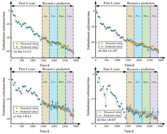
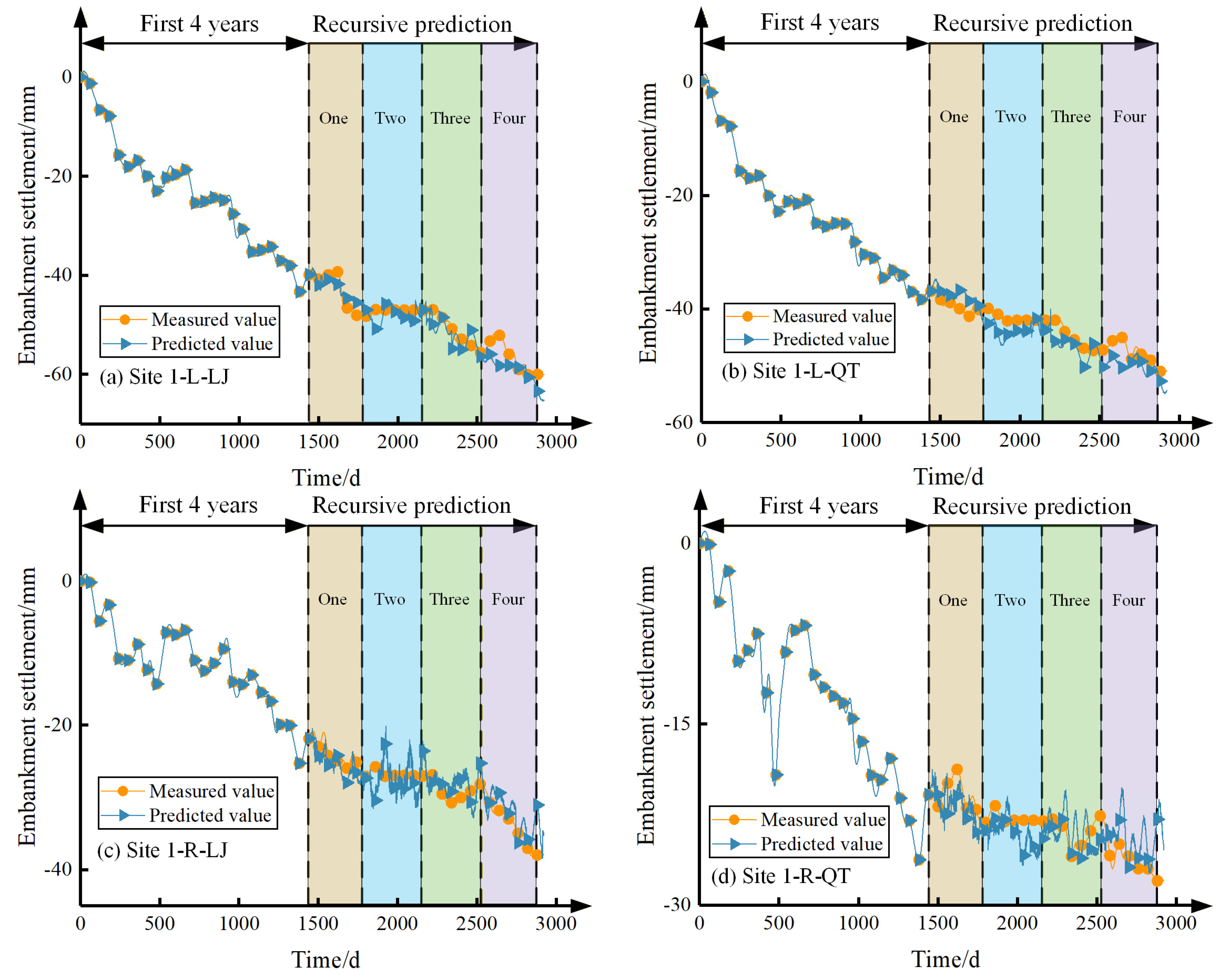
To ensure the accuracy of settlement prediction results for evaluating the serviceability of the embankment, this study first verifies the effectiveness of the dynamic compensation prediction method. The prediction results are shown in Figure 6. Based on data from four monitoring points, the settlement monitoring data from the four years prior to the mutation during which settlement rates remained stable were used as training samples. A four-step dynamic compensation prediction was then conducted with a one-year step size. At each step, the most recent one-year observational data were incorporated, enabling the model to progressively integrate the relatively stable post-mutation settlement patterns, update the settlement trends in real time, and enhance prediction accuracy. The prediction period spans from May 2010 to May 2018. A detailed analysis of each monitoring point is presented below.
Figure 6.
Long-term dynamic recursive prediction results based on monitoring data from the past eight years: (a) left side of embankment at Site 1; (b) left side of abutment at Site 1; (c) right side of embankment at Site 1; (d) right side of abutment at Site 1.
At the left-side monitoring points shown in Figure 6a,b (the left side of the embankment and the left side of the abutment at Site 1), the Mean Absolute Percentage Error (MAPE) values for the four dynamic compensation steps were approximately 3.86% and 4.81%, respectively. The overall prediction errors were relatively low and showed limited fluctuation. Notably, at the left side of the roadbed (Site 1), prediction errors remained low during the first three steps, with only a slight increase in the final step. The overall prediction results were stable and reliable, unaffected by the mutation point, indicating that the dynamic compensation model effectively captured the deformation characteristics and exhibited strong learning capability.
Combined with the analysis of deformation trends, it can be observed that the settlement process in this area follows a relatively smooth, curvilinear descent with clear patterns and low variability. This suggests that the model performs well when applied to stable and simply patterned deformation data. The settlement prediction results also reflect that the cooling measures in this area have achieved favorable cooling and deformation control effects.
In contrast, at the right-side monitoring points shown in Figure 6c,d (i.e., the right side of the roadbed and the right side of the abutment at Site 1), the MAPE values across the four dynamic compensation steps were 6.27% and 6.56%, respectively—significantly higher than those on the left side—and the prediction curves exhibited pronounced fluctuations. The deformation trends in the figures suggest that the original deformation data on the right side are more volatile. When such highly fluctuating and discrete settlement data are used as training samples, the model has more difficulty learning the underlying deformation features and patterns, ultimately resulting in relatively poorer prediction performance at these two monitoring points.
In summary, the prediction results reveal significant differences in settlement trends and model accuracy between the left and right monitoring points, indicating spatial heterogeneity in land settlement. These differences also reflect the varying cooling performance of cooling measures across regions. Therefore, based on limited early-stage deformation monitoring data, this study applies the SAA-GRU-LSTM hybrid time-series dynamic compensation prediction model to dynamically evaluate the operational status and regulatory effectiveness of cooling measures. This assists in determining whether current engineering interventions meet the standards for controlling roadbed settlement. For areas where prediction results indicate ongoing settlement and poor cooling performance of the implemented measures, further engineering reinforcement should be considered promptly to enhance thermal stability and structural safety, thus providing scientific support and technical assurance for the long-term stable operation of transportation infrastructure in permafrost regions.
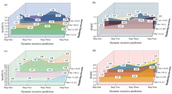
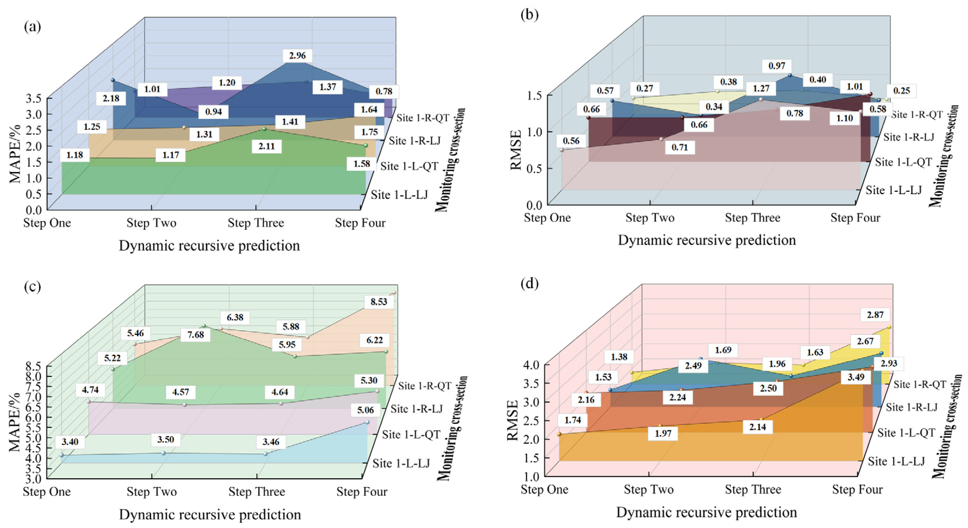
As shown in Figure 7, the error metrics MAPE and RMSE for both the test sets and prediction sets at each step during the dynamic compensation prediction process of the four monitoring points are presented. Taking the dynamic compensation prediction process of the left abutment point at Site 1 as an example, it is found that the MAPE of the test set ranges from 1.17% to 2.11%, while that of the prediction set ranges from 3.40% to 5.30%. Throughout the entire dynamic compensation prediction process, all error metrics remain at relatively low levels and exhibit stable performance on both the test and prediction sets. Combined with the previous analysis of the mean absolute error, it can be further concluded that for settlement deformation data of permafrost embankments characterized by relatively regular deformation trends and small fluctuations, the SAA-GRU-LSTM hybrid time-series prediction model can better learn the deformation features and produce more accurate forecasts.
Figure 7.
Comparison of error evaluation metrics for testing and prediction sets at different time steps during the dynamic recursive prediction process: (a,b) is part of the testing set; (c,d) is part of the prediction set.
Overall, the maximum MAPE for the test set is 2.96%, occurring in the third-step prediction of the right abutment point at Site 1. The maximum MAPE for the prediction set is 8.53%, occurring in the fourth-step prediction of the same point. Both this point and the right embankment point at Site 1 maintain relatively higher error levels on the test and prediction sets. Similarly, the RMSE of the test set ranges from a minimum of 0.25 to a maximum of 1.27, which occur respectively at the first-step prediction of the right abutment point and the third-step prediction of the left embankment point at Site 1. The RMSE of the prediction set ranges from 1.38 to 3.49, occurring at the first-step prediction of the right abutment point and the fourth-step prediction of the left embankment point, respectively.
In summary, comparison of the error metrics among different monitoring points reveals that the stability of the training data itself has a significant impact on prediction accuracy, although all error metrics remain within acceptable ranges. The SAA-GRU-LSTM hybrid time-series dynamic compensation prediction model established in this study can maintain relatively low levels of error metrics even when faced with monitoring data featuring diverse deformation patterns, complex fluctuations, and obvious change points. This not only further demonstrates the accuracy and stability of the hybrid model in evaluating the effectiveness of cooling measures in permafrost regions, but also validates the feasibility of the dynamic compensation prediction method and approach used in this study, as well as its applicability to settlement data containing change points.
3.6. Analysis of Cumulative Error Phenomenon
Furthermore, as shown in Figure 7, a clear accumulation of errors can be observed in the prediction sets during the dynamic compensation prediction process. The following analysis is conducted for each of the four monitoring points. For the left embankment point at Site 1, the MAPE increased from 3.40% to 5.06%, corresponding to an error growth rate of 48.82%, while the RMSE rose from 1.74 to 3.49, showing a rapid error growth rate of 100.57%. At the left abutment point of Site 1, the MAPE increased from 4.74% to 5.30%, with an error growth rate of 11.81%, and the RMSE increased from 2.16 to 2.93, representing an error growth rate of 26.28%. For the right embankment point at Site 1, the MAPE increased from 5.22% to 6.22%, an error growth rate of 19.16%, while the RMSE rose from 1.53 to 2.67, corresponding to an error growth rate of 74.51%. At the right abutment point of Site 1, the MAPE increased from 5.46% to 8.53%, with an error growth rate of 56.23%, and the RMSE rose from 1.38 to 2.87, showing a rapid error growth rate of 107.97%. Overall, the error metrics for all four monitoring points exhibit a generally rapid increasing trend, with the rate of error accumulation accelerating as the number of compensation steps increases.
In summary, the dynamic recursive prediction method adopted in this study results in accumulating errors throughout the prediction process. Furthermore, as the number of prediction steps increases, the rate at which errors accumulate also grows. The fundamental reason is that as each subsequent prediction data point is continually added to the previous step’s data for training, the model continues to learn the deformed features it previously learned during the prediction process. This ongoing process perpetually impacts subsequent recursive predictions, leading to continuous error accumulation. Therefore, dynamic recursive prediction cannot actually continue to predict indefinitely. When errors accumulate to a certain extent, the predicted results deviate significantly from the actual monitored data. In such cases, the predicted values no longer hold reference values. The maximum number of prediction steps within the permissible error range is determined by the stability of the training samples themselves, as well as the sizes of the selected sliding and prediction windows. Therefore, this study follows the principle of dynamic recursive prediction—”short-term predictions for short-term, long-term predictions for long-term”—which not only keeps all error metrics within acceptable limits but also maximizes the size of the prediction window to the greatest extent possible.
3.7. Preliminary Serviceability Evaluation Based on Prediction Results
Based on the dynamic recursive prediction results of the SAA-GRU-LSTM model for the future four years (May 2016 to May 2020), this section conducts a preliminary stability evaluation of the study point according to the serviceability control criteria of the Code for Design of Railway Embankments. The comparative analysis of key indicators against the code thresholds for each monitoring point during the prediction period is presented in Table 2.
Table 2.
Serviceability indicators based on predictions and comparison with code criteria.
The predicted annual settlement rates are well below the 20 mm/year engineering control value, and the accumulated settlements also meet the code requirements. This suggests that the thermosyphon reinforcement measures have been highly effective on this side, and the embankment is in a stable condition. Section 2 evaluated the embankment’s serviceability based on the actual monitoring data from 2010 to 2020, confirming its compliance with design codes and identifying a stabilizing trend post-2015. This section demonstrates that the proposed prediction model, utilizing only early-stage monitoring data, can achieve a scientifically robust serviceability evaluation of the embankment. This capability holds true even when the settlement process exhibits dynamic trend changes or encounters abrupt mutations at certain points in time.
In summary, the proposed dynamic prediction model not only provides numerical forecasts of future settlement but, more importantly, translates these predictions into direct judgments on structural stability. For sections whose predicted future settlement trends (e.g., rates) exceed the stability control thresholds, the model framework can provide early warnings of potential instability, prompting consideration of whether additional reinforcement is needed. This demonstrates the model’s value in supporting decision-making for the operation and maintenance of permafrost engineering structures.
4. Discussion
In this study, due to the influence of multiple factors on permafrost degradation, the settlement process exhibits significant uncertainty. The presence of abrupt change points during settlement poses severe challenges to the accuracy and generalization ability of prediction models, thereby affecting the continuous evaluation of the effectiveness of cooling measures. Traditional machine learning methods typically rely on training data dominated by stable trend segments prior to the change points, making it difficult to effectively capture the non-stationary variations after the changes, which results in prediction outcomes that significantly deviate from actual trends. This issue is further exacerbated when dataset partitioning does not adequately consider the structural characteristics of these abrupt changes, leading to increased prediction errors. Therefore, this paper proposes a dynamic compensation prediction method specifically designed to address the abrupt change features in the settlement process. By continuously incorporating the previous step’s prediction results as new training inputs, the method transforms traditional single-step prediction into a multi-step forecasting process that progressively corrects the prediction trajectory and achieves smooth transitions between trend segments. This approach effectively overcomes the dependency of conventional models on high-quality datasets. Each prediction stage can be viewed as the establishment and iteration of a local sub-model, enabling the model to more flexibly adapt to sudden changes in settlement trends. The results demonstrate that even in the presence of significant abrupt trends, the dynamic compensation prediction method effectively controls prediction bias and achieves accurate settlement predictions for permafrost embankments, providing a more precise, reliable, and engineering-adaptive solution for the continuous evaluation of cooling measure reinforcement effectiveness.
Furthermore, based on the introduction of the dynamic compensation strategy, the model was optimized using the SAA and integrated the advantages of two neural network architectures—GRU and LSTM—to construct a novel hybrid prediction model. This model performed well in predicting settlement in permafrost regions, with error evaluation metrics consistently maintained at low levels. The results indicate that the model possesses strong predictive capability even when faced with highly volatile permafrost settlement data. The established model not only provides decision support for the maintenance and reinforcement of existing permafrost engineering structures but also offers a scientific basis for assessing potential traffic safety risks.
However, the model has two limitations in making long-term predictions. First of all, data collection brings great challenge. Under the influence of extreme weather conditions in permafrost regions, it is relatively difficult to obtain the settlement data in permafrost regions, and the lack of long-term observation data can affect the accuracy of model predictions. Therefore, it is necessary to develop automatic deformation monitoring technology that can operate, monitor and transmit data stably in permafrost regions for a long time. Second, the dynamic recursive prediction method is prone to error accumulation. Research shows that with the increase in the number of dynamic recursive prediction steps, the error increases slowly at first, but then increases almost exponentially. This indicates that this method cannot perform “unlimited” update indefinitely. This phenomenon has important implications for engineering applications: the credible prediction horizon of the model is finite. The rapid accumulation of errors implies that when the prediction step length exceeds a certain limit (approximately 4 years for the medium-term prediction window in this study), the absolute error of the prediction results may become unacceptable, thereby losing its value for guiding long-term maintenance planning. Consequently, in practical engineering applications, this model should be positioned as a medium- to short-term (e.g., 3–5 years) early warning and assessment tool. Based on its reliable results within this window, maintenance authorities can formulate more targeted medium-term inspection and maintenance plans (e.g., scheduling detailed inspections or light reinforcements for sections predicted to be unstable) rather than relying on it for precise forecasts over decades. Future research should seek a better balance between prediction accuracy, window length, and computational efficiency to extend the model’s effective prediction horizon. Third, in terms of the depth of physical interpretation, although the Pettitt test identified a statistically significant change point around 2015, which shows a strong temporal correlation with the delayed cooling effect of the thermosyphon engineering, it remains challenging to conduct a more in-depth decomposition of the physical causes of this change point based on the limited data from a single monitoring section. This includes, for example, accurately quantifying the respective contributions of complex factors such as concurrent climatic fluctuations and the evolution of water-thermal-mechanical coupling processes. Moreover, while this study preliminarily validated the effectiveness of the dynamic compensation strategy under specific data conditions, the systematic dependence of model performance on the scale and quality of early-stage training data has not yet been fully examined. Systematically evaluating how prediction accuracy varies with the “initial information quantity” is crucial for defining the model’s reliability and determining the “minimum monitoring requirements for engineering applications.” This will require verification and analysis in follow-up work using comparative data from multiple climatic zones and different engineering phases. Finally, it must be emphasized that the model is fundamentally data-driven, and its reliable prediction scope is confined to the climate-geotechnical-engineering regime represented by the training data. Directly applying it to predict long-term settlements under extreme, unobserved climatic scenarios or in newly constructed projects with significantly different geological conditions would entail uncertainty and extrapolation risks. Furthermore, integrating numerical modeling frameworks that support early warning and emerging threat mitigation in cold-region infrastructure could help enhance the model’s predictive capability [32,33]. Future work should therefore aim to integrate such modeling tools with enhanced field investigation techniques to improve predictive capacity and engineering applicability under diverse and changing conditions.
5. Conclusions
Addressing the challenges of dynamic changes in the settlement process and scarce physical information in permafrost regions, this study establishes an integrated framework for embankment settlement prediction and serviceability evaluation. The main conclusions are as follows:
(1) The settlement process in thermosyphon-reinforced permafrost embankments is dynamically non-stationary. The Pettitt test identified a statistically significant change point around 2015 across all monitoring points, confirming a major shift in settlement trends and highlighting the need for models that can adapt to such abrupt changes.
(2) The SAA-GRU-LSTM model with a dynamic compensation strategy enables effective mid-term prediction under data-scarce conditions. The hybrid model, trained on limited early-stage data, achieved accurate recursive forecasting and demonstrated a strong capacity to adapt its predictions after the 2015 change point, maintaining acceptable error levels.
(3) The proposed framework integrates prediction with quantitative serviceability evaluation. By directly applying railway embankment design code criteria to model predictions, the study transitions from traditional retrospective analysis to a prospective serviceability assessment, offering a direct link between forecasted behavior and engineering safety standards.
(4) The model serves as a reliable medium-term decision-support tool, with its effective horizon bounded by error accumulation. While the dynamic recursive approach is prone to increasing error over many prediction steps, it establishes a credible early-warning capability for a practical forecast window (e.g., 3–5 years), informing timely maintenance planning.
Author Contributions
Conceptualization, M.Y. and S.Z.; methodology, M.Y. and S.Z.; software, X.L.; validation, Z.F. and Y.R.; formal analysis, M.Y. and S.Z.; investigation, Z.F.; resources, S.Z.; data curation, S.Z.; writing—original draft preparation, M.Y. and S.Z.; writing—review and editing, S.Z.; visualization, X.L. and Y.R.; supervision, S.Z.; project administration, Z.F.; funding acquisition, S.Z. All authors have read and agreed to the published version of the manuscript.
Funding
This research was funded by Natural Science Foundation of Hunan Province of China (grant number 2024JJ6023), the Science and Technology Research and Development Program of China Railway Qinghai-Tibet Group Co., Ltd. (grant number QZ2024-G02), the Open Fund Project of the State Key Laboratory of Green and Long-Life Road Engineering in Extreme Environment (grant number KCJJ2025-03), and the R & D Program of Science and Technology of China Railway Qinghai-Tibet Group Co., Ltd. (QZ2024gldqh-1102).
Data Availability Statement
Data are contained within the article.
Acknowledgments
We sincerely appreciate the editors and reviewers of this journal for their valuable suggestions on this manuscript.
Conflicts of Interest
The authors declare no conflicts of interest. Authors Meng Yuan, Xiaoyue Lin, Zhaojia Fang, and Yuhe Ruan were employed by the company the Second Engineering Company of CCCC Fourth Harbor Engineering Co., Ltd. Author Saize Zhang was employed by the company CCCC First Highway Consultants Co., Ltd.
Abbreviations
The following abbreviations are used in this manuscript:
| QTP | Qinghai–Tibet Plateau |
| QTR | Qinghai–Tibet Railway |
| EBTS | Embankment-Bridge Transition Section |
| SAA | Simulated Annealing Algorithm |
| LSTM | Long Short-Term Memory |
| GRU | Gated Recurrent Unit |
| MAPE | Mean Absolute Percentage Error |
| RMSE | Root Mean Square Error |
| MSE | Mean Squared Error |
References
- French, H.M. The Periglacial Environment; John Wiley & Sons: Hoboken, NJ, USA, 2017. [Google Scholar]
- Nan, Z.; Li, S.; Cheng, G. Prediction of permafrost distribution on the Qinghai-Tibet Plateau in the next 50 and 100 years. Sci. China Ser. D Earth Sci. 2005, 48, 797–804. [Google Scholar] [CrossRef] [Scilit]
- Cheng, G.; Wu, T. Responses of permafrost to climate change and their environmental significance, Qinghai-Tibet Plateau. J. Geophys. Res. Earth Surf. 2007, 112, F02S03. [Google Scholar] [CrossRef] [Scilit]
- O’Neill, H.B.; Smith, S.L.; Burn, C.R.; Duchesne, C.; Zhang, Y. Widespread permafrost degradation and thaw subsidence in northwest Canada. J. Geophys. Res. Earth Surf. 2023, 128, e2023JF007262. [Google Scholar] [CrossRef] [Scilit]
- Liu, H.; Huang, S.; Xie, C.; Tian, B.; Chen, M.; Chang, Z. Monitoring Roadbed stability in permafrost area of Qinghai–Tibet railway by MT-InSAR technology. Land 2023, 12, 474. [Google Scholar] [CrossRef] [Scilit]
- Kondratiev, V.G. Main geotechnical problems of railways and roads in kriolitozone and their solutions. Procedia Eng. 2017, 189, 702–709. [Google Scholar] [CrossRef] [Scilit]
- Zhang, S.Z.; Liu, J.W.; Niu, F.J.; Dong, T.; Pan, X. Research on a wide applicability prediction model for embankments with different settlement patterns in permafrost regions. Cold Reg. Sci. Technol. 2026, 241, 104683. [Google Scholar] [CrossRef] [Scilit]
- Zhang, S.Z.; Wang, Y.G.; Zeng, L.; Luo, J.; Wang, J.; Dong, T.; Niu, F. Long-term deformation rules of railway embankments in permafrost regions: Classification and prediction. Cold Reg. Sci. Technol. 2025, 231, 104425. [Google Scholar] [CrossRef] [Scilit]
- Doré, G.; Niu, F.; Brooks, H. Adaptation methods for transportation infrastructure built on degrading permafrost. Permafr. Periglac. Process. 2016, 27, 352–364. [Google Scholar] [CrossRef] [Scilit]
- Pei, W.; Zhang, M.; Li, S.; Lai, Y.; Dong, Y.; Jin, L. Laboratory investigation of the efficiency optimization of an inclined two-phase closed thermosyphon in ambient cool energy utilization. Renew. Energy 2019, 133, 1178–1187. [Google Scholar] [CrossRef] [Scilit]
- Liu, M.; Ma, W.; Niu, F.; Luo, J.; Yin, G. Thermal performance of a novel crushed-rock embankment structure for expressway in permafrost regions. Int. J. Heat Mass Transf. 2018, 127, 1178–1188. [Google Scholar] [CrossRef] [Scilit]
- Han, U.C.; Choe, C.S.; Hong, K.U.; Han, H. Intelligent back analysis of geotechnical parameters for time-dependent rock mass surrounding mine openings using grey Verhulst model. J. Cent. South Univ. 2021, 28, 3099–3116. [Google Scholar] [CrossRef] [Scilit]
- Luo, J.; Niu, F.; Liu, M.; Lin, Z.; Yin, G. Field experimental study on long-term cooling and deformation characteristics of crushed-rock revetment embankment at the Qinghai–Tibet Railway. Appl. Therm. Eng. 2018, 139, 256–263. [Google Scholar] [CrossRef] [Scilit]
- Chen, L.; Yu, W.; Lu, Y.; Liu, W. Numerical simulation on the performance of thermosyphon adopted to mitigate thaw settlement of embankment in sandy permafrost zone. Cold Reg. Sci. Technol. 2018, 128, 1624–1633. [Google Scholar] [CrossRef] [Scilit]
- Liu, M.H.; Li, G.Y.; Niu, F.J.; Lin, Z.J.; Shang, Y.H. Porosity of crushed rock layer and its impact on thermal regime of Qinghai—Tibet Railway embankment. J. Cent. South Univ. 2017, 24, 977–987. [Google Scholar] [CrossRef] [Scilit]
- Niu, F.; Zhang, S.; Zeng, L.; He, P.; Wang, J.; Dong, T. Settlement trend of embankment–bridge transition section reinforced with thermosyphons in permafrost regions. Transp. Geotech. 2023, 43, 101131. [Google Scholar] [CrossRef] [Scilit]
- TB10001-2016; Code of Railway Subgrade Design. National Railway Administration of People’s Republic of China: Beijing, China, 2016. (In Chinese)
- Kokelj, S.V.; Jorgenson, M.T. Advances in thermokarst research. Permafr. Periglac. Process. 2013, 24, 108–119. [Google Scholar] [CrossRef] [Scilit]
- Memiş, M.A.; Keskin, I.; Demir, S.; Memiş, Ş.U. Machine learning-based prediction of permafrost degradation and its implications on geotechnical infrastructure: A comprehensive review. AI Civ. Eng. 2025, 4, 28. [Google Scholar] [CrossRef] [Scilit]
- Gama, J.; Žliobaitė, I.; Bifet, A.; Pechenizkiy, M.; Bouchachia, A. A survey on concept drift adaptation. ACM Comput. Surv. (CSUR) 2014, 46, 1–37. [Google Scholar] [CrossRef] [Scilit]
- Yang, E.; Wang, K.; He, J.; Liu, K.; Wang, J.; Zhang, H.; Qiu, Y. Settlement prediction of a high embankment based on non-linear regression and neural network algorithm. Transp. Geotech. 2025, 50, 101443. [Google Scholar] [CrossRef] [Scilit]
- Graves, A. Long short-term memory. In Supervised Sequence Labelling with Recurrent Neural Networks; Springer: Berlin/Heidelberg, Germany, 2012; pp. 37–45. [Google Scholar]
- Černý, V. Thermodynamical approach to the traveling salesman problem: An efficient simulation algorithm. J. Optimiz. Theory Appl. 1985, 45, 41–51. [Google Scholar] [CrossRef] [Scilit]
- Kirkpatrick, S.; Gelatt, C.D., Jr.; Vecchi, M.P. Optimization by simulated annealing. Science 1983, 220, 671–680. [Google Scholar] [CrossRef] [Scilit]
- Metropolis, N.; Rosenbluth, A.W.; Rosenbluth, M.N.; Teller, A.H.; Teller, E. Equation of state calculations by fast computing machines. J. Chem. Phys. 1953, 21, 1087–1092. [Google Scholar] [CrossRef] [Scilit]
- Laarhoven, P.J.M.; Aarts, E.H.L. Simulated Annealing: Theory and Applications; Springer: Dordrecht, The Netherlands, 1987. [Google Scholar]
- Vasilakos, C.; Tsekouras, G.E.; Kavroudakis, D. LSTM-Based Prediction of Mediterranean vegetation dynamics using NDVI time-Series data. Land 2022, 11, 923. [Google Scholar] [CrossRef] [Scilit]
- Gao, S.; Huang, Y.; Zhang, S.; Han, J.; Wang, G.; Zhang, M.; Lin, Q. Short-term runoff prediction with GRU and LSTM networks without requiring time step optimization during sample generation. J. Hydrol. 2020, 589, 125188. [Google Scholar] [CrossRef] [Scilit]
- Hyndman, R.J.; Koehler, A.B. Another look at measures of forecast accuracy. Int. J. Forecast. 2006, 22, 679–688. [Google Scholar] [CrossRef] [Scilit]
- Hong, J.; Liang, F.; Yang, H.; Zhang, C.; Zhang, X.; Zhang, H.; Wang, W.; Li, K.; Yang, J. Multi-forword-step state of charge prediction for real-world electric vehicles battery systems using a novel LSTM-GRU hybrid neural network. Etransportation 2024, 20, 100322. [Google Scholar] [CrossRef] [Scilit]
- Hong, J.; Wang, Z.; Chen, W.; Wang, L.Y.; Qu, C. Online joint-prediction of multi-forward-step battery SOC using LSTM neural networks and multiple linear regression for real-world electric vehicles. J. Energy Storage 2020, 30, 101459. [Google Scholar] [CrossRef] [Scilit]
- Liberotti, R.; Cluni, F.; Gusella, V.; Lourenço, P.B. The Green Tape project. ‘In falso’ walls strengthening through natural FRCM innovative techniques. Eng. Struct. 2025, 345, 121459. [Google Scholar] [CrossRef] [Scilit]
- Cluni, F.; Faralli, F.; Gusella, V.; Liberotti, R. X-rays CT and Mesoscale FEM of the Shot-Earth Material. In Shot-Earth for an Eco-friendly and Human-Comfortable Construction Industry; Tarantino, A.M., Cotana, F., Viviani, M., Eds.; Springer Tracts in Civil Engineering: Berlin/Heidelberg, Germany, 2023; pp. 25–44. [Google Scholar]

Disclaimer/Publisher’s Note: The statements, opinions and data contained in all publications are solely those of the individual author(s) and contributor(s) and not of MDPI and/or the editor(s). MDPI and/or the editor(s) disclaim responsibility for any injury to people or property resulting from any ideas, methods, instructions or products referred to in the content. |
© 2026 by the authors. Licensee MDPI, Basel, Switzerland. This article is an open access article distributed under the terms and conditions of the Creative Commons Attribution (CC BY) license.